Combining Information Across Diverse Sources: The II-CC-FF Paradigm

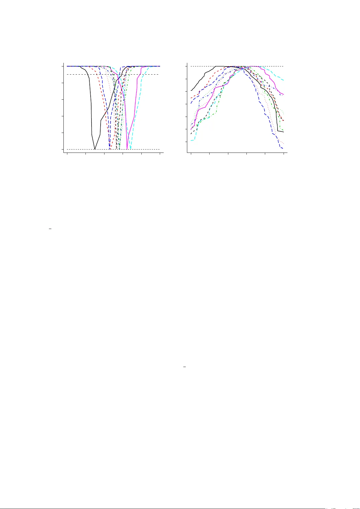
Com bining Information Across Div erse Sources: The I I-CC-FF P aradigm June 2020 C´ eline Cunen and Nils Lid Hjort 1 Departmen t of Mathematics, Univ ersity of Oslo Abstract W e introduce and develop a general paradigm for combining information across diverse data sources. In broad terms, suppose ϕ is a parameter of interest, built up via comp onen ts ψ 1 , . . . , ψ k from data sources 1 , . . . , k . The prop osed sc heme has three steps. First, the Inde- pendent Inspection (I I) step amounts to inv estigating each separate data source, translating statistical information to a conﬁdence distribution C j ( ψ j ) for the relev ant fo cus parameter ψ j associated with data source j . Second, Conﬁdence Con version (CC) tech niques are used to translate the conﬁdence distributions to conﬁdence log-likelihood functions, say ℓ conv ,j ( ψ j ). Finally , the F ocused F usion (FF) step uses relev an t and context-driv en tec hniques to construct a conﬁdence distribution for the primary focus parameter ϕ = ϕ ( ψ 1 , . . . , ψ k ), acting on the com bined conﬁdence log-likelihoo d. In traditional setups, the I I-CC-FF strategy amounts to v ersions of meta-analysis, and turns out to be comp etitiv e a gainst state-of-the-art methods. Its potential lies in applications to harder problems, how ever. Illustrations are presen ted, related to actual applications. Key wor ds: com bining information, conﬁdence distributions, conﬁde nce likelihoo ds, focused fusion, hard and soft data, meta-analysis. 1 Com bining information and the I I-CC-FF sc heme Our pap er concerns the statistical task of combining information across diﬀerent and p erhaps very div erse data sources. This is of course a long-standing theme in statistics, with papers going bac k to Karl Pearson (cf. Simpson & Pearson (1904)); see Sc hw eder & Hjort (2016, Ch. 13) for bac kground and a general discussion of themes traditional ly sorted under the bag-word meta- analysis, along with further basic references. The present pap er aims at proposing and dev eloping a certain paradigm, which we call the I I-CC-FF metho d, meant to b e p o wer fully applicable for ranges of situations far b ey ond the usual simpler setups. W e will explain the role and nature of the Indep enden t Inspection (I I), Conﬁdence Conv ersion (CC), F o cused F usion (FF) steps b elo w. A special case worth considering ﬁrst is the textb ook setup where y 1 , . . . , y k are independent estimators of the same quan tity ψ , and where y j ∼ N( ψ , σ 2 j ), with known standard deviations σ j . 1 An easy exercise in minimising v ariances sho ws that the optimally balanced o verall estimator is b ψ = P k j =1 y j /σ 2 j P k j =1 1 /σ 2 j ∼ N  ψ ,  k X j =1 1 /σ 2 j  − 1  . (1.1) A natural extension, though harder to analyse to full satisfaction, is when y j ∼ N( ψ j , σ 2 j ), with the individual means ψ j diﬀering according to a N( ψ 0 , τ 2 ) distribution. F or this type of random eﬀects mo del, one wishes clear inference strategies for b oth the ov erall mean ψ 0 and lev el of v ariation τ . W e return to this particular problem in Sections 6.1, 8.1, and 9.1. Man y problems of modern statistics in volving combining information are m uch more compli- cated than the situations sk etched ab o ve, ho wev er. Sometimes one needs to combine ‘hard’ data, with clear measuremen ts from con trolled exp erimen ts, etc., with ‘soft’ data, asso ciated with infor- mation more lo osely connected to the parameters of primary in terest, p erhaps via measuremen t errors or surrogate v ariables. In addition there might b e prior distributions a v ailable, via sub ject matter experts, but only for some of the parameters at play , not enough to mak e it into a clear Ba yesian analysis. F or our developmen t of I I-CC-FF w e ha ve attempted to think fundamentally and generally ab out combination of information problems. Our framewor k encompasses known meta-analysis metho ds, but we aim at tac kling new and more chall enging problems as w ell. P arts of the meta-analysis literature are quite narro w, with sp eciﬁc methods for sp eciﬁc problems. In that light we hop e our more general approach will be useful. In reasonably general terms, assume there is a parameter ϕ of clear interest, related to param- eters ψ 1 , . . . , ψ k , either via a deterministic function ϕ = ϕ ( ψ 1 , . . . , ψ k ) or via some type of random eﬀect distribution, where such a ϕ might b e a parameter related to a bac kground distribution of the ψ j . Suppose further that data source y j pro vides information p ertaining to ψ j . F or the sake of clear presentation, w e let the ψ j b e one-dimensional here. Our I I-CC-FF approac h for reachi ng inference statements for the ov erall fo cus parameter ϕ can then b e sc hematically set up as follo ws: ⋄ II, Indep endent Insp e ction : Data source y j is used, via appropriate mo dels and analyses, to yield a conﬁdence distribution C j ( ψ j , y j ) for the main in terest parameter associated with study j . ⋄ CC, Conﬁdenc e Conversion : The conﬁdence distribution is conv erted into a log-likeli ho o d function for this main parameter of int erest for study j , sa y ℓ conv ,j ( ψ j ). ⋄ FF, F o cuse d F usion : In the ﬁxed eﬀect case, the combined conﬁdence log-likelihoo d func- tion ℓ fus ( ψ 1 , . . . , ψ k ) = P k j =1 ℓ conv ,j ( ψ j ) is used to reach fo cused fusion inference for ϕ = ϕ ( ψ 1 , . . . , ψ k ). With random eﬀects, the fusion inv olv es the computation of an int egral. W e do make use of certain subscripts in our pap er, mean t as helpful signp osting. The subscript ‘con v ’ is for likelihoo d functions coming out the CC-step; ‘fus’ relates to the FF-step; while ‘prof ’ and ‘cprof ’ are used for the proﬁle log-lik eliho od and its corrected version (see Section 5.2). The extent to whic h some or all of these steps will be relativ ely straigh tforward or rather complicated to carry out dep ends to a high degree on the sp ecial features of the giv en source com- bination problem. The steps are not ‘isolated’ or fully separated, but often related. In Section 5.1 w e provide a standardised version of I I-CC-FF, with a generic recip e to follow, but we will see that in many cases one could or should b e more careful ab out the v arious steps. In situations where the statistician has all the raw data and the particular models used for analysing the diﬀerent sources of 2 information, the CC step is in a conceptual sense not diﬃcult, as the required log-lik eliho od parts ma y b e wor ked out from ﬁrst principles. In v arious situations confronting the modern statistician this is rather more diﬃcult, ho wev er, as one migh t hav e to base one’s analysis on summary mea- sures, directly or indirectly giv en via other p eople’s work, rep orts and publications. The I I-CC-FF paradigm is mean t to b e p o werfully applicable in such situations to o. A p ertinen t question is whether or why there is a need for speciﬁc methods for combination of information in the ﬁrst place; in a suitable sense, all of statistics concerns combination of information. One might therefore ask why there ev en exist subﬁelds such as meta-analysis, and sp eciﬁc framew ork aimed at combination of information suc h as our own. So isn’t meta-analysis just analysis? Tw o related responses are as follo ws. (i) Sometimes the full sets of data are not a v ailable, with access only to summaries or partial summaries. Issues here are storage, the practicalities of other people’s ﬁles, priv acy concerns, etc. (ii) Sometim es it migh t be easier, conceptually or practically , to analyse the diﬀerent sources or studies separately ﬁrst, and then com bine these pieces of summarised information. Also, a statistical prediction is that mo dern statistics to an increasing degree will b e concerned with such issues and challenge s, ﬁnding and organising bits and pieces of information across diﬀeren t sources, with a need to reach conclusions based on these pieces. After a motiv ating illustration, b elo w, w e start in Section 2 with a brief review of conﬁdence distributions (CDs), whic h are essen tial for the Indep enden t Inspection (II) part of the programme. W e then pro ceed with giving detail s related to the basics of Conﬁdence Con version (CC) in Section 3 and F o cused F usion (FF) in Section 4. In Section 5 we pro vide a standard v ersion of our I I- CC-FF framework, and inv estigate some pitfalls and solutions. In Section 6 we inv estigate the use of our II-CC-FF sc heme in well-established meta-analysis situations, and in Section 7 connections with other CD based approaches are explored. F urther p erformance and comparison issues are examined in Section 8, both via sim ulations and decision theoretic risk functions. There, w e ﬁnd that I I-CC-FF metho ds are comp etitiv e in sev eral traditional meta-analysis settings. The three step I I-CC-FF machinery is then seen in action through four applications laid out in Section 9. Motiv ating illustration The follo wing concrete illustration, which has certain features placing it outside the usual meta- analysis setups and metho ds, shows the three steps of the I I-CC-FF at work, but with a minimum of details. The nonstandard asp ect for this illustration is partly that diﬀerent studies of the same statistical question hav e rep orted diﬀeren t summary measures – six st udies (call them t yp e A) h av e reported summary statistics based on contin uous outcomes, while ﬁve other studies (which we call t yp e B) rep orted summaries based on a binary outcome. More crucially , the focus parameter β in question, a regression co eﬃcien t related to the diﬀerence b et ween treatments , is not iden tiﬁable, and hence cannot b e estimated directly , for the t yp e B studies. In fact, these type B studies only inform us ab out a certain β /σ , where also σ is not ident iﬁable, or estimable, from those studies. Also, the raw data, for these studies, are not av ailable. The data employ ed here were ﬁrst analysed in Whitehead et al. (1999); related problems ha ve been treated in Dominici & Parmigiani (2000) and Liu et al. (2015). W e hav e eleven randomised trials inv estigating the use of ox yto cic drugs during labour and its p oten tial eﬀect on p ostpartum blo od loss. Eac h study has tw o groups of patients, a treatmen t group receiving oxytocic drug and a con trol group receiving no drugs of that t yp e. T aking y i,j to 3 b e the blo od loss for patien t i in study j , we may use the simple mo del y i,j = α j + β z i,j + ε i,j , with the ε i,j independent and N(0 , σ 2 ), and with z i,j an indicator v ariable, equal to 0 for patients in the control group and 1 for patien ts in the treatment group. Here β is the treatment eﬀect and the parameter of main int erest. F or the six type A trials, we hav e the mean and the empirical standard deviation of the blo od loss in the tw o groups of patien ts. With the simple normal model abov e, these four summary statistics are suﬃcie nt for eac h trial, and we thus hav e access to the full log-lik eliho o d ℓ A,j ( β , α j , σ ) for each contin uous tr ial j . F or the ﬁv e t yp e B trials, ho wev er, we merely ha ve counts of the num ber of patien ts in each group having a bloo d l oss of more or less than 500 ml. These n umbers constitute a non-suﬃcient summary; w e thus ha ve less information in these studies compared to the contin uous ones, and log-likelihoo d functions not able to inform on β directly , only on β /σ . More speciﬁcally , based on the normal model ab o ve, w e obtain a probit-t yp e log-lik eliho od for these binary trials, sa y ℓ B ,j ( θ , γ j ), with γ j = (500 − α j ) /σ and θ = β /σ . Ha ving made these modelling assumptions, the steps in the II-CC-FF recipe follo w straight- forw ardly . Using the log-likelihoo d functions described ab o ve, we can, b y metho ds describ ed in the next section, construct c onﬁdenc e curves for the parameter of in terest for each of the studies. −150 −100 −50 0 0.0 0.2 0.4 0.6 0.8 1.0 β confidence cur v e Figure 1.1: Conﬁdence curv es for the treatment eﬀect in the six continuous trials (dashed, blac k). In red, the conﬁdence curv e combining all the elev en studies. The horizontal red line marks the 95% conﬁdence level. The median conﬁdence estimate is − 83 . 7 ml, with 95% in terv al [ − 94 . 4 , − 73 . 1]. The CC step is simple in this case, with no extra work required, since the log-likelihoo d functions were used in the construction of the conﬁdence curves for eac h study . In other situations w e migh t hav e to carry out the con version from conﬁdence statemen ts to log-lik eliho od functions in wa ys describ ed in Section 3. Via arguments explained in more detail in the next section, we reac h log-lik eliho od con tributions ℓ A, prof ,j ( β , σ ) for the cont inuous studies and ℓ B , prof ,j ( β /σ ) for 4 the binary studies. In the FF step these are summed, to reac h FF : ℓ fus ( β , σ ) = 6 X j =1 ℓ A, prof ,j ( β , σ ) + 5 X j =1 ℓ B , prof ,j ( β /σ ) . Next we proﬁle out σ and obtain the ﬁnal com bined conﬁdence curve by cc ∗ ( β , all data) = Γ 1  2 { max ℓ fus ( β , b σ ( β )) − ℓ fus ( β , b σ ( β )) }  , with Γ 1 ( · ) the c.d.f. of a χ 2 1 . In Figure 1.1, the thic k red curv e is this combined conﬁdence curv e. It is clearly narrow er than all the individual curves and placed roughly in the middle of them, as w e would exp ect. The combined inference clearly demonstrates that o xyto cic drugs reduce postpartum blo od loss, whic h is in agreement with the conclusions in Whitehead et al. (1999). Here we hav e zo omed in on β as the fo cus parameter, to pinpoint precisely ho w muc h the tw o groups diﬀer in blo od loss. F or clinicians it might be of more direct interest to consider the probabilities for ha ving a p ostpart um blo od loss greater than a threshold, like 500 ml, for the t wo groups, and then fo cus on the o dds ratio, say ρ . Our approach can easily accommodate such an analysis to o, with ρ rather than β in the FF step, yielding a ﬁgure similar to Figure 1.1, but now for ρ . The I I, CC, FF steps are not intended to form a unique recip e, as there are individual v ariations, dep ending on the application at hand. In the FF step ab o ve the log-lik eliho od contributions for type A and t yp e B information were arrived at via proﬁling of the fuller log-lik eliho ods constructed under the auspices of the regression mo del we started out with. In other applications this would not b e p ossible, and there would b e a need to conv ert CC information to log-lik eliho ods, a theme w e examine in Section 3. 2 Indep enden t Inspection: conﬁdence distributions Suppose Y j denotes a set of random observ ations from data source j , stemming from a mo del with parameter θ j , t ypically m ultidimensional, and with ψ j = ψ ( θ j ). F or the ease of presentati on, we let ψ j b e a one-dimensional fo cus parameter for no w, but in general combination situations it will t ypically b e multidimensional. A c onﬁdenc e distribution (CD) C j ( ψ j , y j ) for this fo cus parameter from source j has the properties (i) i t is a cumulati ve distribution function (c.d.f.) in ψ j , for each y j , and (ii) at the true v alue θ 0 , with asso ciated true v alue ψ 0 = ψ ( θ 0 ), the distribution of C j ( ψ 0 , Y j ) is uniform on the unit interv al. F rom this follo ws, under standard contin uity and monotonicit y assumptions, that P θ 0 { C − 1 j (0 . 05 , Y j ) ≤ ψ 0 ≤ C − 1 j (0 . 95 , Y j ) } = 0 . 90 , etc., i.e . [ C − 1 j (0 . 05 , y j, obs ) , C − 1 j (0 . 95 , y j, obs )] is a 90% conﬁdence interv al for ψ j , where y j, obs denotes the observed dataset. Th us the CD C j ( ψ j , y j, obs ), qua random c.d.f., is a compact and con venien t represen tation of conﬁdence interv als at all lev els, and indeed a p o we rful inference summary . A close relative is the c onﬁdenc e curve , which we tend to prefer as a p ost-data graphical summary of information for fo cus parameters, deﬁned as cc j ( ψ j , y j, obs ) = | 1 − 2 C j ( ψ j , y j, obs ) | . (2.1) It points to its cusp p oin t, the median conﬁdence point estimate b ψ j, 0 . 50 = C − 1 j ( 1 2 , y j, obs ), and the t wo ro ots of the equation C ( ψ j , y j, obs ) = α form a conﬁdence interv al with this conﬁdence lev el. 5 Degrees of asymmetry are easier to sp ot and to con vey using the conﬁdence curve than with the cum ulative CD itself; cf. illustrations in Section 9. W e also note that the random cc j ( ψ j , Y j ) has a uniform distribution, at the true p osition in the parameter space, since | 1 − 2 U | is uniform when U is. Indeed P θ 0 { cc j ( ψ 0 , Y j ) ≤ α } = α, for each α, (2.2) at the true parameters of the model. The conﬁdence curv e is arguably a more fundamen tal concept than the con ﬁdence distribution, as there are cases where a natural cc j ( ψ j , Y j ) ma y be constructed, with a v alid (2.2), even when conﬁdence regions are formed by disjoin t interv als (as with multimodal log-lik eliho od functions). F or an extensive treatmen t of CDs, their constructions in diﬀerent types of setup, prop erties and uses, see Sch weder & Hjort (2016), and the review pap er Xie & Singh (2013), with ensuing discussion con tributions. The scop e and broad applicabilit y of CDs are also demonstrated in a collection of pap ers published in the sp ecial issue Infer enc e With Conﬁdenc e of the journal Journal of Statistic al Planning and Infer enc e , 2018 (Hjort & Sch weder, 2018). Here we shall merely p oin t to tw o imp ortan t and broadly useful w ays of constructing a conﬁdence distribution, for a fo cus parameter ψ j , based on data from a model with a m ultidimensional parameter θ j . The ﬁrst is to rely on an approximat ely normally distributed estimator, if a v ailable, sa y b ψ j ∼ N( ψ j , κ 2 j ), and with standard deviation w ell estimated with an appropriate b κ j . Then, with Φ( · ) as usual denoting the c.d.f. of the standard normal, C j ( ψ j , y j ) = Φ(( ψ j − b ψ j ) / b κ j ) is an appro ximately correct CD, ﬁrst-order large-sample correct under weak regularit y conditions. In particular the estimator used can b e the maxim um likelihoo d one (ML), say b ψ j, ml , but other estimators are allo wed to o in this simple construction. The second is based on the proﬁled log-lik eliho od function ℓ prof ,j ( ψ j ) = max { ℓ j ( θ j ) : ψ ( θ j ) = ψ j } , which leads to the deviance function D j ( ψ j ) = 2 { ℓ prof ,j ( b ψ j, ml ) − ℓ prof ,j ( ψ j ) } = 2 { ℓ prof ,j, max − ℓ prof ,j ( ψ j ) } . (2.3) As laid out in Sch weder & Hjort (2016, Chs. 2, 3), the Wilks theorem with v ariations then lead naturally to cc j ( ψ j , y j ) = Γ 1 ( D j ( ψ j )) , (2.4) with Γ ν ( · ) denoting the c.d.f. of a χ 2 with degrees of freedom ν . Typically , the second metho d (2.4) leads to a b etter calibrated conﬁdence curv e than the the simpler metho d men tioned ﬁrst. 3 Conﬁdence Con ve rsion: from conﬁdence to lik eliho ods Sev eral w ell-explored metho ds, with appropriate v ariations and amendmen ts, lead from like liho o d functions to CDs and conﬁdence curv es; cf. again seve ral chapters of Sch w eder & Hjort (2016). Sometimes the CC step comes almost for free, in cases where the statistician can compute sa y log-lik eliho od proﬁles from ra w data, or from suﬃcient statistics, for the given mo dels. But in some cases the CC step of the II-CC-FF paradigm requires metho ds for going the other wa y , from CDs or conﬁdence curves to log-lik eliho od information, and this is more inv olved. Among the complications is that diﬀere nt experimental protocols, with ensuing diﬀeren t CDs, might be ha ving the same log-lik eliho od functions, so the link b et ween conﬁdence and likelihoo d is not one-to-one. 6 Sc hw eder & Hjort (2016, Ch. 10) dev elop and discuss this topic at some length. F or the present purposes we shall b e conten t with what w e call the chi-squar e d inversion , associated with (2.4) ab o v e. Assume that all our information ab out a parameter ψ j from source j comes in the form of the conﬁdence curve cc j ( ψ j , y j ). Then we can obtain a conﬁdence log-likelihoo d contribution from source j by the follo wing form ula ℓ conv ,j ( ψ j ) = − 1 2 Γ − 1 1 (cc j ( ψ j , y j )) . (3.1) If the conﬁdence curv e has b een constructed via the second general metho d presented in the previous section, see (2.4), w e will of course simply get back the proﬁled log-lik eliho od function. The CC step therefore onl y comes in to pla y when conﬁdence curve are constructed via non-standard methods, as we will see in Applications 9.2 and 9.3, or when the only av ailable information from source j is the conﬁdence curv e itself and we do not kno w exactly how it w as constructed. When a CD is av ailable, rather than a conﬁdence curve, one can use the normal c onversion ℓ conv ,j ( ψ j ) = − 1 2 { Φ − 1 ( C j ( ψ j , y j )) } 2 . This is equiv alen t to the recip e in (3.1), when the conﬁdence curv e has b een constructed via cc j ( ψ j , y j ) = | 1 − 2 C j ( ψ j , y j ) | . A relev ant p oin t here is that one often constructs a conﬁdence curve cc j ( ψ j , y j ) directly , not alwa ys via (2.1), making (3.1) a more v ersatile to ol. The normal con version conﬁdence likelihoo d is also what Efron (1993) prop osed, for coming from conﬁdence to likelihoo d, via diﬀeren t arguments and for diﬀeren t purp oses; see also Efron & Hastie (2016, Ch. 11). F or details on how well the chi-squared inv ersion metho ds works, in diﬀerent scenarios, see Section 4.3. In some situations one is able to construct a CD for source j via a one-dimensional stati stics T j , instead of using the general metho d from (2.4). Then one may use exact c onversion to obtain the conﬁdence log-lik eliho od. When the statistic has a contin uous distribution, the exact conv ersion of the CD C j ( ψ j , T j ), see Sch weder & Hjort (2016, Ch. 10), is ℓ conv ,j ( ψ j ) = log | ∂ C j ( ψ j , t ) /∂ t | . 4 F ocused F usion: from full lik eliho od to fo cus parameter Suppose no w that the II and CC steps hav e b een successfully carried out, leading to conﬁdence log-lik eliho od contributions ℓ conv ,j ( ψ j ) from information sources j = 1 , . . . , k . Dep ending on the application and its context we might then b e interested in either a ﬁxed eﬀect approach, with the main focus parameter ϕ is a function of the ψ j , or a random eﬀect approach, where we in tro duce an additional lay er of heterogeneity through a mo del for the ψ j . W e will treat the ﬁxed eﬀect case ﬁrst. 4.1 Fixed eﬀects fusion Assuming the information sources to b e indep enden t, the ov erall conﬁdence log-likelihoo d function is ℓ fus ( ψ 1 , . . . , ψ k ) = P k j =1 ℓ conv ,j ( ψ j ). When fo cused inference is wished for, for a fo cus parameter ϕ = ϕ ( ψ 1 , . . . , ψ k ), the natural wa y forw ard is, again, via proﬁling: ℓ fus , prof ( ϕ ) = max { ℓ fus ( ψ 1 , . . . , ψ k ) : ϕ ( ψ 1 , . . . , ψ k ) = ϕ } . By the Wilks theorem directly , or b y v ariations of the arguments and details used to prov e suc h theorems (cf. Sc hw eder & Hjort (2016, App endix)), the o verall deviance function D ∗ ( ϕ ) = 2 { ℓ fus , prof ( b ϕ ) − ℓ fus , prof ( ϕ ) } 7 tends, at the true parameter p osition and with increasing information volume, to a χ 2 1 . Here b ϕ is the ML, maximising the proﬁled log-likelihoo d. Hence cc ∗ ( ϕ, all data) = Γ 1 ( D ∗ ( ϕ )) (4.1) is the outcome of the three step I I-CC-FF machine, a conﬁdence curve for the fo cus parameter. In Section 4.3 we will come back to some discussion on the meaning of ‘increasing information v olume’ in a combination context. In situations where the ψ j represen t the same fo cus parameter, common across sources, the sch eme ab o ve simpliﬁes. 4.2 Random eﬀects fusion In our II-CC-FF setting, we use the term ‘ran dom eﬀects’ when w e wish to in tro duce an extra la yer of heterogeneity in the fusion step. This is more easily presen ted when assuming that ψ 1 , . . . , ψ k are scalars. In the random eﬀects case we do not assume that all ψ j are equal but rather that they come from some underlying distribution. In the most canonical case, this distribution will b e gov erned by some ov erall mean parameter ψ 0 and some spread parameter τ ; sp eciﬁcally w e could hav e ψ j ∼ N( ψ 0 , τ 2 ). The parameter of main interest may b e either the o verall mean, or the spread, or p erhaps a quantile, dep ending on the conte xt. W e prop ose the following general solution for II-CC-FF with random eﬀects. Suppose the ψ j are mo delled as coming from a bac kground densit y f ( ψ j , κ ), say , where the κ could b e a cen tre and a spread parameter, as for ( ψ 0 , τ ) in the normal case. Then, using the conﬁdence log-likelihoo ds ℓ conv ,j ( ψ j ) from each source, we deﬁne the fusion log-likelihoo d to be ℓ fus ( κ ) = k X j =1 log h Z exp { ℓ conv ,j ( ψ j ) } f ( ψ j , κ ) d ψ j i . (4.2) W e would usually need to proﬁle again, dep ending on what we are interested in, sa y the centre ψ 0 or spread τ for the case of a normal model for the ψ j . T o produce our ﬁnal conﬁdence curv e we will often use the Wilks approximation. This I I-CC-FF solution requires the computation of in tegrals. Sometimes numerical in tegration routines in R work well enough, other times w e will make use of the so-called T emplate Mo del Builder pack age (TMB) and its Laplace approximations in order to compute the in tegral (Kristensen et al., 2016). 4.3 Wilks theorems for conv ersion and fusion There are c hi-squared appro ximation metho ds at work at sometimes several levels in our I I-CC- FF scheme. F or some applications the c hi-squared inv ersion method (3.1) is crucial, as for the nonparametric CDs for quan tiles in Application 9.3, and for other situations what matters more migh t be the chi-squared appro ximation of the FF step (4.1). Limit distribution results securing suc h χ 2 1 limits are collectiv ely referred to as Wilks theorems, with diﬀerent setups of regulatity conditions. W e refrain from setting up lists of precise regularit y conditions here, as applications of the theory would inv olve diﬀeren t t yp es of situations, but we give brief p oin ters to relev ant methods and literature, as follo ws. First, regarding (3.1) and conv ersion to log-lik eliho ods, b oth the exact log-likelihoo d and the in version approximation are guaran teed to b e close to the negativ e quadratic − 1 2 ( ψ j − b ψ j, ml ) 2 / b κ 2 j , for the appropriate b κ j , b y argumen ts asso ciated with classical large-sample calculus. This would 8 include asymptotic normality of the ML estimator and indeed the traditional Wilks theorem, see Sc hw eder & Hjort (2016, Ch. 2 and Appendix). The resulting approximations are typically goo d also when the data information volume is small, as long as the underlying mo dels are smooth in their parameters. Second, the arguments and methods p oin ted to also entail that the FF inference method (4.1) is large-sample close to that of minimising the relev ant P k j =1 ( ψ j − b ψ j, ml ) 2 / b κ 2 j under ϕ = ϕ ( ψ 1 , . . . , ψ k ) constraints. F or such minim um chi-squared methods, precise Wilks theorems are given in F erguson (1996, Section 23). Regularit y conditions there are of the t yp e where the n umber of information sources k is kept mo derate and ﬁxed, but with steadily more data for each. Imp ortan tly , limiting normality of estimators, along with limiting χ 2 1 results for deviances, can also b e deriv ed in the rather diﬀerent setups with small data v olume for each source, but where the n umber k increases. A case in p oin t is where ϕ = b t ψ is linear in the ψ j , with estimator b ϕ = b t b ψ , and the FF step is large-sample equiv alent to D ∗ ( ϕ ) = ( ϕ − b ϕ ) 2 / P k j =1 b 2 j b κ 2 j . This tends to a χ 2 1 for increasing k , under mild regularit y conditions. 5 I I-CC-FF v ersions The ov erall ob jective of the I I-CC-FF is to construct a v alid conﬁdence curv e for each parameter ϕ of particular interest, typically of the form ϕ = ϕ ( ψ 1 , . . . , ψ k ), incorporating the relev an t information in all the sources. The framework we hav e presen ted so far has not intended to pro vide a single clear-cut recip e for doing such analyses in practice. Below one such concrete recipe is presented, ho wev er, which we call the standard I I-CC-FF metho d, and which ma y b e used for a wide range of mo dels and data. The standard framework has limitations, which w e will discuss, and which will serv e as a starting point for the presen tation of some partial solutions, and more ﬁn e-tuned v ersions of the I I-CC-FF sc heme. These discussions also highlight v arious imp ortan t general issues with methods for com bination of information whic h are relev ant also outside the I I-CC-FF framewor k. 5.1 Standard I I-CC-FF The sc heme to be describ ed now requires that w e ha ve the full data a v ailable, or suﬃcien t sum- maries, from all sources. The statistical work starts by deciding on one or more parameters of particular interest, in vol ving relev ant parameters ψ 1 , . . . , ψ k from the k sources. These might b e parameter vectors (i.e. need not b e one-dimensional), they might diﬀer from source to source, but ma y also contain common parameters across sources. ⋄ II, Indep endent Insp e ction : analyse each source j separately . Assume a parametric mo del for the observ ations and put up the likelihoo d function. Proﬁle out the source-sp eciﬁc nuisanc e parameters, and obtain ℓ prof ,j ( ψ j ). ⋄ CC, Conﬁdenc e Conversion : in this case w e already ha ve th e log-likelihoo d proﬁles from eac h source, so the conﬁdence con version is simple, using the ℓ prof ,j ( ψ j ) directly . ⋄ FF, F o cuse d F usion : here we wan t to obtain a conﬁdence curve for the parameter of ov erall in terest ϕ . Depending on the situation, (i) if ϕ is assumed to b e the same across sources or a function of some source-speciﬁc parameters, sum the ℓ conv ,j and then proﬁle again if necessary; (ii) if some comp onen t of the ψ j are assumed to come from some common distribution, use the random eﬀects solution presented ab o ve, and then proﬁle again if needed. 9 W e then obtain ℓ fus , prof ( ϕ ), and in b oth cases w e use the Wilks appro ximation to pro duce the ﬁnal, com bined conﬁdence curve cc ∗ ( ϕ, data). As for conﬁdence curv es in general, we consider the metho d to work if the ﬁnal com bined conﬁdence curv e cc ∗ ( ϕ ) has the right co verage properties, either exactly or appro ximately , as p er (2.2). If the ﬁnal combined conﬁdence curv e do es not ha ve the correct cov erage properties, this ma y b e due to t wo related problems: (1) the proﬁling in either the I I or the FF step has gone wrong; and (2) the distribution of the deviance (based on the proﬁle log-lik eliho od) is far from a χ 2 1 , i.e. the Wilks appro ximation is not v alid. Problem (2) is related to the issues discussed in Section 4.3 and will usually disapp ear when either k or the n j increase. In situations with little data, the Wilks appro ximation can sometimes b e ameliorated using relativ ely simple to ols, like the Bartlett correction; see for instance Sc hw eder & Hjort (2016, Chs. 7, 8) for a discussion on suc h ﬁne-tuning methods and second-order approx - imations. F urther, in some situations one ma y be able to deriv e and sim ulate the distribution of the deviance exactly , and thus bypass the use of the Wilks approximation altogether. W e will see examples of suc h I I-CC-FF v ersions in Sections 6.1 and 9.1. Problem (1) is related to the proﬁling and the presence of n uisance parameters. In situa- tions with nuisance parameters using the proﬁle log-likelihoo d can lead to “ineﬃcient and ev en inconsisten t estimates” (McCullagh & Tibshirani, 1990). As w e see abov e, the standard I I-CC-FF method ma y often require tw o rounds of proﬁling: ﬁrst in the I I step where we might proﬁle out the sour c e-sp e ciﬁc n uisance parameters, and sometimes in the FF step where we might proﬁle out shar e d n uisance parameters (which are shared by the k sources). If we hav e ‘large sources’, i.e. the sample size n j of each source is large, we can safely proﬁle in the II step. If some or all the sources are small, how ever, one should b e more careful. Sp eciﬁcally , the proﬁling might go wrong and w e illustrate this situation with a famous example in App endix C, the Neyman-Scott problem. Shared n uisance parameters can b e of diﬀerent kinds, and here w e will particularly concern ourselv es with nuisance parameters arising from the random eﬀect distribution in the FF step. F or example, if we ha ve ψ j ∼ N( ψ 0 , τ 2 ) and our fo cus parameter is ψ 0 , then τ is a shared nuisance parameter of that type. If the num b er of sources k is large we can safely proﬁle, while if k is small w e ma y need to resort to some of the corrections described next. Often w e ha ve b oth source-sp eciﬁc and shared nuisance parameters. In that case, we ideally need to hav e a large num b er of large sources in order to produce v alid CDs with the default proﬁling-based metho d. Note that in these cases, if k is too small, large sources will not necessarily help. Conv ersely , if the n j are too small, a large k will not in general b e able to remedy the mistak es coming from proﬁling in the I I step. 5.2 Corrections to the log-likelihoo d proﬁle There is a large literature concerning corrections or modiﬁcations to the proﬁle lik eliho od. The diﬀeren t corrections appearing in the literature hav e v arying p erformance and complexity; see for instance Barndorﬀ-Nielsen (1986), Cox & Reid (1993), Diciccio & Efron (1992), Stern (1997), DiCiccio et al. (1996). There is also a whole subﬁeld of integrated lik eliho od metho ds with partly similar aims, see Berger, Liseo & W olp ert (1999). A thorough inv estigation of all these metho ds is outside the scop e of this article, and we will therefore only present one rather simple, somewhat limited solution. Alternative metho ds might w ork b etter, or at least in a more general setting, but these are often more complicated to compute. 10 In Cox & Reid (1987), the authors present what we will term the simple Cox –Reid correction. This is p ossibly the easiest correction to compute among those suggested ab o v e. It can b e consid- ered a special case of the correction in the general mo diﬁed proﬁle likelihoo d of Barndorﬀ-Nielsen, but the simple Co x–Reid correction is limited to situations with orthogonal parameters (i.e. that the oﬀ-diagonal terms in the expected information matrix are equal to zero). Assume w e ha ve a scalar parameter of interest ψ and some vector of n uisance parameters λ . As usual, the proﬁle log-lik eliho od for ψ is deﬁned as ℓ prof ( ψ ) = ℓ ( ψ , b λ ( ψ )), where b λ ( ψ ) is the ML estimate of λ for eac h ﬁxed ψ v alue. The simple Cox–Reid correction gives the follo wing modiﬁcation of the proﬁle log-lik eliho od, ℓ cprof ( ψ ) = ℓ prof ( ψ ) − 1 2 log[det J λλ ( ψ , b λ ( ψ ))] (5.1) where J λλ ( ψ , b λ ( ψ )) = − ∂ 2 ℓ ( ψ , λ ) / ( ∂ λ∂ λ t ) is the observed information for the λ components, ev aluated at ( ψ , b λ ( ψ )). The simple Co x–Reid correction can b e used b oth in the I I and FF steps, for mo dels with orthogonal parameters. W e illustrate the use of the Co x–Reid correction in the I I step in the Appendix Section C. In the FF step, corrections ma y b e necessary when there are shared n uisance parameters arising from a random eﬀect distribution. In particular, we propose that this correction should readily be applied when then random eﬀect distribution is assumed to b e normal. Here, the correction should b e particularly notable for small k . W e will present some Co x–Reid corrections in a classic mo del for random eﬀect meta-analysis in Section 6. 5.3 Optimal CD metho ds F or some parameters in exp onen tial families, w e can bypass the standard II-CC-FF, and its p o- ten tial problems, b y making use of the follo wing alternative metho d which is muc h more pow erful, pro duci ng optimal CDs . In our I I-CC-FF setting, this metho d migh t come into play b oth in the I I step and the FF step, see the application in Section 6.2. F or ease of presentation, we present the optimal conﬁdence metho d in the case where all the k sources inform on a common fo cus parameter ψ = ψ 1 = · · · = ψ k . This constitutes a situation where the metho d is used in the ﬁnal FF step. Suppose again that ψ is the focus parameter, and that w e ha ve m nuisance parameters γ 1 , . . . , γ m , whic h ma y be both source-speciﬁc or shar ed across all k sources. Suppose also that the log-likelihoo d function at work, based on information sources y 1 , . . . , y k , can b e written in the form ℓ ( ψ , γ 1 , . . . , γ m ) = ψ A + γ 1 B 1 + · · · + γ m B m − d ( ψ , γ 1 , . . . , γ m ) + h ( y 1 , . . . , y k ) , (5.2) where A and B 1 , . . . , B m are statistics, i.e. functions of the data collection, with observ ed v al- ues A obs and B 1 , obs , . . . , B m, obs , and with m often bigger than k . Then, under mild regularity conditions, there is an o verall most pow erful CD, namely C ∗ ( ψ , y ) = P ψ { A ≥ A obs | B 1 = B 1 , obs , . . . , B m = B m, obs } . That this C ∗ ( ψ , y ) indeed dep ends on ψ but not on the γ j parameters is part of the result and the construction. T o illuminate the exact meaning of ‘most p o w erful’ in this setting, one needs to consider the theory for loss and risk functions for CDs dev elop ed in Sc hw eder & Hjort (2016, Ch. 5). Conﬁdence p o w er is measured via the risk function r ( C, ψ , γ ) = E ψ ,γ Z Γ( ψ cd − ψ ) d C ( ψ cd , Y ) , (5.3) 11 for any conv ex nonnegativ e Γ( · ) with Γ(0) = 0. The random mechanism inv olv ed in the expectation here is a t wo-stage op eration; ﬁrst data y , go verned by the ( ψ, γ ) held ﬁxed, are used to generate the CD C ( ψ , y ), and then ψ cd is a random dra w from this distribution. Int uitively , a lo w conﬁdence risk means that the CD in question is tight around true v alue of ψ , while CDs which are less concen trated around the true v alue will hav e a higher risk. A CD with low conﬁdence risk should therefore b e expected to pro duce narrow conﬁdence in terv als (but keeping the correct cov erage), and p oin t estimates with little bias. W e will see the conﬁdence risk concept at work in Section 8.3. 6 Meta-analysis As mentioned in the small start example (1.1), some common meta-analysis metho ds ﬂow more or less directly from the I I-CC-FF framework. In addition, the framewor k also invites more general, principled and non-standard solutions some which we will explore in this section. F urther, we will inv estigate connections b et ween I I-CC-F F and a couple of widely encoun tered meta-analysis methods. W e will start with a discussion of the basic random eﬀect mo del, b efore we go on to the famous case of meta-analysis of 2 × 2 tables. 6.1 The basic random eﬀect mo del The most canonical type of random eﬀect meta-analysis, whic h we term the basic random eﬀect mo del, starts with k indep enden t estimators y 1 , . . . , y k aiming at the parameters ψ 1 , . . . , ψ k , with y j | ψ j ∼ N( ψ j , σ 2 j ), and ψ j ∼ N( ψ 0 , τ 2 ). Usually the source-sp eciﬁc standard deviations σ j are assumed kno wn. The literature treating this model is enormous, see for instance Langan et al. (2019) and P artlett & Riley (2017) and references therein. Note that lik eliho od-based method for the basic random eﬀect mo del, ev en exploring higher order corrections, hav e b een inv estigated earlier, see for instance Hardy & Thompson (1996) and Noma (2011). F or a more general likelihoo d approac h see O’Rourke (2008). When assuming kno wn σ j , the integral in (4.2) has an explicit solution and the standard I I-CC-FF solution will rely on the following log-lik eliho od function ℓ ( ψ 0 , τ ) = k X j =1 n − 1 2 log( σ 2 j + τ 2 ) − 1 2 ( y j − ψ 0 ) 2 σ 2 j + τ 2 o , where w e proﬁle out either ψ 0 or τ dep ending on whic h parameter is of main in terest. The conﬁdence curv es for ψ 0 and τ will point at the standard ML estimators, and the ensuing conﬁdence in terv als will be very similar to solutions which ha v e b een inv estigated in some of the references men tioned abov e. These solution are reasonably go od when k is not to o small, see also Section 8.1, but may b e impro ved up on. Langan et al. (2019) ﬁnds, for instance, that the ML estimator for τ has relatively p oor performance in terms of bias and mean squared error. W e can attempt to impro ve on the standard II-CC-FF solution using the Co x–Reid correction. First we will consider the case where ψ 0 is the parameter of main interest, then the full com bined proﬁle likelihoo d from the FF step b ecomes ℓ fus ,c prof ( ψ 0 ) = k X j =1 n − 1 2 log( σ 2 j + b τ 2 ( ψ 0 )) − 1 2 ( y j − ψ 0 ) 2 σ 2 j + b τ 2 ( ψ 0 ) o − 1 2 log k X j =1 n − 1 2 1 ( σ 2 j + b τ 2 ( ψ 0 )) 2 + ( y j − ψ 0 ) 2 ( σ 2 j + b τ 2 ( ψ 0 )) 3 o . (6.1) 12 The ﬁrst part of the formula is the ordinary proﬁle log-likelihoo d, the second part the simple Cox– Reid correction. W e obtain the combined conﬁdence curv e using the Wilks approximati on. This correction has b een obtained by diﬀeren tiating with resp ect to τ 2 in (5.1); note that a somewhat diﬀeren t correction term w ould ha ve b een obtained if w e had diﬀerentiated with respect to τ . W e ha ve not seen this solution anywhere in the literature, and we inv estigate its p erformance in Section 8.1. In this situation τ is a ‘b order parameter’, as the proﬁled ML estimate b τ ( ψ 0 ) can b e zero with p ositi ve probability . This happ ens precisely when k X j =1 1 σ 2 j n ( y j − ψ 0 ) 2 σ 2 j − 1 o ≤ 0 , (6.2) and if this takes place there is an in terv al of such ψ 0 v alues. The correction term will then exp erien ce non-smoothness at the end p oin ts of that interv al. T o av oid this non-smo othn ess issue, where the rationale b ehind the Cox–Reid correction term do es not easily apply , we set the entire correction term to zero when (6.2) takes place for some ψ 0 . The cor rection term should b e esp ecially important when there are few studies and the heterogeneity b et ween them is large. W e can consider a v ariation of (6.1) in the case of the individual sources hav e few measure- men ts, which means that the σ j estimates become uncertain. The II-CC-FF can then pro vide more sophisticated solutions. In the I I step, we ha ve exact CDs for eac h ψ j based on the Student’s t distribution, which we can conv ert to a conﬁdence log-likelihoo d by exact conv ersion in the CC step. F or the FF step, we use the general random eﬀect method from (4.2), either with n umerical in tegration or using the TMB pack age. Corrections in b oth the I I and FF step may b e considered, but we hav e not fully inv estigated these options y et. Rather than fo cusing on the ov erall mean, as w e did ab o ve, one may b e interested in the o verall spread τ . F rom the ab o ve, w e hav e direct and Co x–Reid corrected log-likelihoo d proﬁles ℓ fus , prof ( τ ) = − 1 2 A k ( τ ) and ℓ fus , cprof ( τ ) = − 1 2 B k ( τ ), with A k ( τ ) = k X j =1 h log( σ 2 j + τ 2 ) + { y j − b ψ 0 ( τ ) } 2 σ 2 j + τ 2 i and B k ( τ ) = A k ( τ ) + log  k X j =1 1 σ 2 j + τ 2  , with the proﬁled ML estimator b ψ 0 ( τ ) = P k j =1 b ψ j / ( σ 2 j + τ 2 ) / P k j =1 1 / ( σ 2 j + τ 2 ) for eac h given τ . One might recognise the − 1 2 B k ( τ ) as the log-likelihoo d asso ciated with the so-called restricted ML or REML estimator for τ , see for instance Langan et al. (2019). The link b et we en the Cox–Reid correction (and more general corrections) and the REML pro cedure has been known for some time, see Durban & Currie (2000) and also Cox & Reid (1987), but is p ossibly under-appreciated in the meta-analysis literature. The ab o ve leads to t wo deviance functions, using the direct and the corrected log-lik eliho od proﬁles, D k, ml ( τ ) = A k ( τ ) − A k ( b τ ml ) and D k, cml ( τ ) = B k ( τ ) − B k ( b τ cml ) , with b τ ml and b τ cml the minimisers of A k ( τ ) and B k ( τ ). The distribution of y j − b ψ 0 ( τ ) do es not depend on the underlying ψ 0 , which means that D k, ml ( τ ) and D k, cml ( τ ) hav e distributions only depending on the candidate v alue τ . Thus we ha ve w ell-deﬁned and exact conﬁdence curves for τ , cc ml ( τ ) = P τ { D k, ml ( τ ) ≤ D k, ml , obs ( τ ) } and cc cml ( τ ) = P τ { D k, cml ( τ ) ≤ D k, cml , obs ( τ ) } . (6.3) W e make use of these conﬁdence curve metho ds in Application 9.1. The Wilks t yp e chi-squared appro ximation w orks well for mo derate to large v alues of k , but not for τ small, which often might 13 b e the parameter region of primary in terest, as for the application pointed to. Hence we need to compute the tw o conﬁdence curv es via simulations, with a high num ber of D k, ml ( τ ) and D k, cml ( τ ) generated for eac h candidate v alue τ . In the normal-normal set-up ab o v e, the parameters are orthogonal, but w e suggest that one could use the simple Cox–Reid correction ev en if the model for the observ ations in each source is non-normal. Supp ose we are in a setting like in (4.2), and assume that the random eﬀect distribution is normal, with the parameter of main interest b eing the ov erall mean ψ 0 . Inside each source we can ha ve any (regular) mo del. In a simple normal mo del, the Cox–Reid correction when proﬁling out the v ariance τ 2 w ould be equal to − log { b τ ( ψ ) } . W e propose to routinely use the follo wing corrected likelihoo d proﬁle construction in this type of random eﬀect setting, ℓ fus ,c prof ( ψ 0 ) = k X j =1 n log h Z exp { ℓ conv ,j ( ψ j ) } 1 b τ ( ψ 0 ) φ  ψ j − ψ 0 b τ ( ψ 0 )  d ψ j io + log { b τ ( ψ 0 ) } , (6.4) where b τ ( ψ 0 ) is the ML estimate of τ for eac h ﬁxed ψ 0 v alue and φ is the standard normal density . The orthogonality of ψ 0 and τ in the full (in tegrated) distribution do es not necessarily hold, but it w ould hold if the sources w ere large, since then ℓ conv ,j ( ψ j ) abov e will approac h a normal lik eliho od. W e therefore consider formula (6.4) to b e an appro ximate correction for the situation when k is small, but the n j are suﬃcien tly large. In fact the correction term in (6.4) is a sp ecial case of the correction term in (6.1) when the σ j go to zero (which of course corresp onds to n j increasing to wards inﬁnity). W e in vestigate this idea in the situation of meta-analysis of 2 × 2 tables, see Section 8.2. 6.2 Meta-analyses of 2 × 2 tables In meta-analyses of 2 × 2 tables, each study seeks to compare the probability of observing a certain binary even t in the control group and in the treatment group. The counting v ariables Y 0 ,j and Y 1 ,j indicate how man y patien ts hav e experienced the ev ent in each group in study j . These v ariables are usually mo delled as pairs of binomials, Y 0 ,j ∼ binom( m 0 ,j , p 0 ,j ) and Y 1 ,j ∼ binom( m 1 ,j , p 1 ,j ), with subscript ‘1’ indicating treatment and ‘0’ con trol, and the sample sizes in eac h group are denoted b y m 0 ,j and m 1 ,j . The most common measure for the treatment eﬀect is the o dd s ratio, or equiv alently , the log o dds ratio ψ j . F or that eﬀect measure it is conv enien t to express the ev ent probabilities in the control and treatmen t groups as p 0 ,j = exp( θ j ) / (1 + exp( θ j )), and p 1 ,j = exp( θ j + ψ j ) / (1 + exp( θ j + ψ j )). Each study , or source, has a speciﬁc n uisance parameter θ j , go verning the even t probabilit y in the control group. W e will ﬁrst treat the ﬁxed eﬀect case where the log o dds ratios are assumed common across all sources, ψ 1 = · · · = ψ k = ψ , before w e come to the random eﬀect case in the next paragraph. The information av ailable in each source depends on the binomial sample sizes m 0 ,j and m 1 ,j , and on the even t probabilities. If the num ber of studies increases while the size of each study stays constant, it is known that the ML estimator is inconsisten t (Breslow, 1981), and w e can exp ect that the standard I I-CC-FF method will not wor k w ell. Also, the simple Co x–Reid correction t o the proﬁle in eac h source is not immediately av ailable b ecause ψ j and θ j are not orthogonal. Ho wev er, there exists an optimal CD for the common ψ based on the theory from Section 5.3, C opt ( ψ , data) = P ψ ( B k > b | z 1 , . . . , z k ) + 1 2 P ψ ( B k = b | z 1 , . . . , z k ) . (6.5) Here, z j = y 0 ,j + y 1 ,j and B k = P k j =1 Y 1 ,j . The CD is obtained by sim ulating the distribution of B k giv en Z 1 , . . . , Z k . The second part of (6.5) is a half-correction. Note also that we similarly 14 ha ve an optimal CD for ψ j within each source, C opt ,j ( ψ j , y 0 ,j , y 1 ,j ) = P ψ ( Y 1 ,j > y 1 ,j | z j ) + 1 2 P ψ ( Y 1 ,j = y 1 ,j | z j ) . (6.6) This CD is simple to compute as Y 1 ,j | Z j has an eccentric h yp ergeometric distribution. Note that this CD is v ery closely related to the method known as Fisher’s exact test (Fisher, 1954). Starting from (6.6) for each source in the I I step, w e can obtain an appro ximation to the optimal solution in (6.5) whic h is faster to compute and also lends itself to a natural random eﬀect extension, as we will see. In the CC step, we use exact conv ersion to obtain the conﬁdence log-likelihoo ds ℓ conv ,j ( ψ j ) = log g j ( y 1 ,j , ψ j ), where g j ( y 1 ,j , ψ j ) =  m 0 ,j z j − y 1 ,j  m 1 ,j y 1 ,j  exp( ψ j y 1 ,j ) P z j u =0  m 0 ,j z j − u  m 1 ,j u  exp( ψ u ) for y 1 ,j = 0 , 1 , . . . , min( z j , m 1 ,j ) (6.7) is the density function of the eccen tric h yp ergeometric distribution. W e sum these conﬁdence log- lik eliho ods to get ℓ fus ( ψ ) = P k j =1 ℓ conv ,j ( ψ j ), ﬁnd the ML estimate b ψ and the deviance, and use the Wilks appro ximation: cc ∗ ( ψ , data) = Γ 1 (2 { ℓ fus ( b ψ ) − ℓ fus ( ψ ) } ) . (6.8) Ev en though there is some lev el of approximation in thi s solution, it tends to work w ell, see Section 8.2. F rom this approximate ﬁxed eﬀect approac h w e ﬁnd a natural extension to random eﬀects. As- suming that the log-o dd ratios from the diﬀerent sources come from a common normal distribution, w e hav e the follo wing fusion log-likelihoo d for the ov erall parameters, ℓ fus ( ψ , τ ) = k X j =1 log n Z g j ( y 1 ,j , ψ j ) 1 τ φ  ψ j − ψ τ  d ψ j o , (6.9) where g j ( y 1 ,j , ψ j ) is the density function of the eccen tric h yp ergeometric distribution, p oin ted to ab o v e. If we are mainly interested in ψ 0 , we proﬁle out τ and use the Wilks approximation. If the heterogeneit y is big or the num b er of sources is small we add the appro ximate Cox–Reid correction log b τ ( ψ ) from (6.4) to the proﬁle log-likelihoo d. In applications, we computed the integral using the TMB pack age. This approac h seems promising with goo d cov erage properties in sim ulations (Section 8.2). 7 Other com bination methods based on CDs There is a steadily growing literature on com bination of information with CDs. Here we wil l brieﬂy discuss metho ds b y Singh et al. (2005) and Liu et al. (2015). These CD approaches are sometimes collected under the same um brella, called F usion Learning (Cheng et al., 2017). W e start by discussing the approac h of Singh et al. (2005), v alid when all conﬁdence com- p onen ts relate to a common fo cus parameter. Supp ose that independent information sources y 1 , . . . , y k giv e rise to CDs for the same parameter, say C 1 ( ψ , y 1 ) , . . . , C k ( ψ , y k ). A general w ay of combining these in to a single ov erall CD has b een prop osed and work ed with by Singh et al. (2005), later on applied in v arious contexts by Xie et al. (2011), Xie & Singh (2013), Liu et al. (2014b), and others. The starting p oin t is that under the true state of aﬀairs, the Φ − 1 ( C j ( ψ , Y j )) are indep enden t standard normals, from the basic prop erties of CDs; here Φ( · ) again denotes the 15 c.d.f. for the standard normal. Hence P k j =1 w j Φ − 1 ( C j ( ψ , Y j )) is also standard normal, when the w eights w j are such that P k j =1 w 2 j = 1. This again implies that ¯ C ( ψ , y ) = Φ  k X j =1 w j Φ − 1 ( C j ( ψ , y j ))  (7.1) is a CD for ψ , using the combine d dataset y = ( y 1 , . . . , y k ). The idea generalises to other basic distributions than the normal, but then the required con volutions b ecome less tractable. F or the prototype situation associated with (1.1), the individual CDs take the form C j ( ψ , y j ) = Φ(( ψ − y j ) /σ j ), and the general (7.1) recip e yields ¯ C ( ψ , y ) = Φ  k X j =1 w j ( ψ − y j ) /σ j  . Some considerations then lead to the b est of these linear combinations , with w eights w j proportional to 1 /σ j and P k j =1 w 2 j = 1. This indeed agrees with the standard method (7.1). Recipe (7.1) requires nonrandom weigh ts w j , and these could in v arious cases b e fruitfully tak en as prop ortional to 1 / √ m j , with m j the sample size asso ciated with data source y j . In man y other situations the balance is more delicate, how ever, p erhaps demanding nonrandom w eights, of the t yp e b w j estimating an underlying optimal but not observ able w j, 0 . Problems work ed with in Liu et al. (2014b) are of this type. In suc h cases recip e (7.1) is not entirely appropriate and is rather to b e seen as an appro ximation, asso ciated with conﬁdence int erv als with approximate lev els of conﬁdence. The approac h describ ed abov e yields approximativ e solutions for the basic normal-normal random eﬀect mo del, partly help ed by the fact that the unconditional densit y in that case has an explicit normal form, y j ∼ N( ψ 0 , σ 2 j + τ 2 ). It is not clear ho w the metho d in Xie et al. (2011) can incorporate more general random eﬀect mo dels, how ev er. Under the ‘F usion learning’ um brella there are other metho ds. The method in Liu et al. ( 2015) ma y be termed a ‘conﬁdence density method’ and can b e considered as a sp ecial case of I I-CC- FF, as w e will see. The metho d is proposed for a ﬁxed eﬀect setting, but where the studies may diﬀer in rep orted outcomes, in measured co v ariates, or ha ve source-sp eciﬁc nuisance parameters. Th us, some of the studies may only contai n indirect information ab out the parameter of in terest. Let θ be the full parameter vector for all the studies and γ j = M j ( θ ) the parameters in study j , with M j denoting a known mapping function. Liu et al. (2015) summarise the information in eac h source with multiv ariate normal CDs, C j ( γ j , y j ), transform these to conﬁdence densities c j ( γ j , y j ) = ∂ C j ( γ j , y j ) /∂ γ j , which are then m ultiplied into a combined conﬁdence density , whic h informs on the full θ . The authors stress that the approach is general in the sense that it can b e used with a wide range of parametric mo dels for the sources. This generalit y is ac hiev ed b ecause the authors assume that the num b er of observ ations in each source increases to inﬁnit y . The normal CDs for eac h study only requires the estimated parameter v ector b γ j and estimated co v ariance matrix b Σ j for b γ j , and the authors therefore highlight that the approach only needs summary statistics r ather than the full data. Also, they pro ve that their approac h is asymptoti cally equally eﬃcient as a traditional lik eliho od approac h using the full data. F or location parameters in normal mo dels the conﬁdence densit y and conﬁdence likelihoo d are prop ortional. The approach in Liu et al. (2015) can therefore b e considered a special case of I I-CC-FF. Sometimes the conﬁdence densit y might b e easier to obtain than the exact conﬁdence 16 log-lik eliho od, and could b e used also in connection with I I-CC-FF. Ho wev er, one migh t need to be careful, as this approac h could in troduce mistakes. The conﬁdence density is equal to ∂ C ( ψ , T ) /∂ ψ , while the exact conﬁdence likelihoo d tak es the deriv ativ e with resp ect to T , as we sa w in Section 3. The diﬀerence b et ween the conﬁdence densit y and conﬁdence lik eliho od will b e the most pronounced when the sample sizes are small, with the diﬀerence going a wa y with increasing sample sizes. 8 P erformance ev aluations The main b eneﬁt of our I I-CC-FF framework is its general nature and wide applicability , and in the next section w e will therefore demonstrate the use of I I-CC-FF in several non-standard com bination situations. Still, we also require that methods coming out of I I-CC-FF should b e comp etitiv e against other methods from the literature when applied to t ypical com bination situations, for example meta-analysis settings. Here we will study the performance of I I-CC-FF metho ds in tw o v ery classical situations: ﬁrst in the basic random eﬀect mo del and then in the meta-anal ysis of 2 × 2 tables. Both of these types of meta-analyses w ere discussed in Section 6, along with some notation whic h will b e used in this section to o. Finally , in the last subsection we will study conﬁdence risk functions for some II-CC-FF schemes, compared to other CD combi nation metho ds, in a particular simpliﬁed example. 8.1 The basic random eﬀect mo del W e hav e in vestigated some of the methods from Section 6.1 with a sim ulation study inspired by Langan et al. (2019). W e treat the setting where ψ 0 is the parameter of main interest. In that setting Langan et al. (2019) found that conﬁdence in terv als computed by the Hartung-Knapp- Sidik- Jonkman metho d were the clear winners in terms of cov erage prop erties. That metho d uses the traditional inv erse-v ariance metho d for the p oin t estimator, and computes conﬁdence interv als based on the t-distribution and the follo wing v ariance formula, V ar HKSJ b ψ 0 = P k j =1 ( b ψ j − b ψ 0 ) 2 / ( b σ 2 j + b τ 2 ) ( k − 1) P k j =1 1 / ( b σ 2 j + b τ 2 ) . This form ula requires one to plug-in an estimator for τ and for this we used the REML estimator, as recommended b y Langan et al. (2019). W e will compare this state-of-the-art metho d with our standard I I-CC-FF metho d, and the I I-CC-FF metho d using the corrected log-likelihoo d proﬁle in (6.1). W e will also include the metho d for the basic random eﬀect mo del whic h comes out of the CD com bination framework of Xie et al. (2011) . This method is implemen ted in the gmeta pac k age (Y ang et al., 2016). See App endix A for more details. W e let ψ 0 = 0 . 5 and consider t wo v alues for the b et ween-study heterogeneit y , τ = 0 . 09 for a scenario with little heterogeneit y and τ = 0 . 44 for a scenario with large heterogeneit y . F urther, we c ho ose σ j = 2 / √ m j with m j ∼ unif(30 , 50), and inv estigate four v alues for the num ber of studies, 5, 10, 20, 50. W e generated 10000 meta-analyses for eac h k v alue. F or a single meta-analysis, ψ j and σ j w ere estimated using their ordinary estimators in eac h of the k studies (even though all the methods assume that the σ j are kno wn). F or each metho d, w e recorded the cov erage rate of 95% conﬁdence interv als, the width of these in terv als, and p oin t estimates for ψ 0 . 17 0.88 0.92 0.96 1.00 cov erage ● ● ● ● ● ● ● ● 0.2 0.4 0.6 0.8 1.0 mean width ● ● ● ● ● ● ● ● ● ● Hartung−Knapp−Sidik−Jonkman gmeta standard II−CC−FF II−CC−FF with correction τ = 0.09 0.88 0.92 0.96 1.00 number of studies cov erage 5 10 20 50 ● ● ● ● ● ● ● ● 0.2 0.4 0.6 0.8 1.0 1.2 1.4 number of studies mean width 5 10 20 50 ● ● ● ● ● ● ● ● τ = 0.44 Figure 8.1: Sim ulation results for the basic random eﬀect model. The left plot gives the realised cov erage rate of 95% conﬁdence interv als, the right plot giv es the median width of these interv als. The results in the top row are for a scenario with small b et ween-study heterogeneity , while in the bottom row the b et ween-study heterogeneit y is large. The conﬁdence interv als from the Hartung-Knapp-Sidik-Jonkman method hav e p erfect cov er- age rate for almost all k v alues in both scenarios (Figure 8.1), whic h is consisten t with results in Langan et al. (2019). The CD metho d from Xie et al. (2011) has v ery go od p erformance in the sce- nario with small heterogeneity , but severe under-cov erage in the scenario with large heterogeneit y . The standard I I-CC-FF metho d has a similar problem in that scenario, but the I I-CC-FF version with corrected proﬁle likelihoo d obtains cov erage rates close to the nominal 0.95. Both I I-CC- FF versions are sligh tly conserv ative in the small heterogeneit y scenario, but obtain nonetheless conﬁdence interv als of similar mean width as the Hartung-Knapp-Sidik-Jonkman interv als. The four methods pro duce virtually iden tical p oin t estimates for ψ 0 . All in all w e ﬁnd the I I-CC-FF method to hav e almost equally go od p erformance as the state-of-the-art metho d. In scenarios with lo w heterogeneity the correction to the proﬁle likelihoo d is not imp ortan t, while it is crucial in scenarios with large b et ween-study heterogeneit y . 8.2 Meta-analyses of 2 × 2 tables W e will in v estigate b oth the ﬁxed eﬀect and random eﬀect cases. Our sim ulation set-ups are inspired b y tw o recen t pap ers with extensive simulation studies: Piaget-Rossel & T aﬀ´ e (2019) for the ﬁxed eﬀect case and Jackson et al. (2018) for the random eﬀects case. With ﬁxed eﬀects, we will inv estigate three common eﬀect measures: the (log) o dds ratio deﬁned in Section 6, the (log) risk ratio, exp( ψ j ) = p 1 ,j /p 0 ,j , and the risk diﬀerence, ψ j = p 1 ,j − p 0 ,j . With random eﬀects, we will only treat the o dds ratio, how ever. Piaget-Rossel & T aﬀ ´ e (2019) focus on meta-analyses with rare ev ents, i.e. where b oth the treatmen t and control group ha ve low ev ent probabilities and where there may be many studies with zero ev ents. The o verall conclusion of the pap er was that the Man tel-Haenszel method had the b est p erformance among the metho ds that were considered. This method is applicable to all 18 three eﬀect measures men tioned ab o ve, and Piaget-Rossel & T aﬀ ´ e (2019) found that it pro duced conﬁdence interv als with goo d cov erage prop erties, and p oin t estimates with relatively small bias. The Mant el-Haenszel is a w ell-established metho d, which w as originally proposed in 1959 (Man tel & Haenszel (1959) and extended in Rothman et al. (2008)). The metho d oﬀers explicit estimators for the log odds ratio, log risk ratio and risk diﬀerence, as well as expressions for the v ariance of these estimators. Conﬁdence in terv als are computed using the W ald appro ximation. W e will compare some v ariants of our I I-CC-FF scheme with the Man tel-Haenszel metho d. W e will also include metho ds review ed in Liu et al. (2014a). These metho ds are based on exact tests and fall in to the unifying CD framework of Singh et al. (2005) which w e described in Section 7. F or the o dds ratio and risk diﬀerence, these CD metho ds hav e b een implemented in the gmeta pack age (Y ang et al., 2016); for the risk ratio a related exact metho d is implement ed in the exactmeta pac k age (Y u & Tian, 2014). See App endix A for more details. F or all three eﬀect measures w e will make use of the standard II-CC-FF pro cedure which consists of proﬁling out the n uisance parameters in eac h source, summing the log-lik eliho od proﬁles ,and then using the Wilks appro ximation to obtain a conﬁdence curve for ψ , from which we can extract conﬁdence interv als and point estimates. F or the odds ratio case we will include tw o additional v ariants that can b e said to fall under the I I-CC-FF umb rella: the optimal CD method giv en in (6.5) and the II-CC-FF metho d using exact con version , whic h w e giv e in (6.8). This I I-CC-FF v ersion resem bles the standard I I-CC-FF pro cedure, but a voids the proﬁling step by making use of the conditional log-likelihoo d for ψ j , in (6.7). W e sim ulated datasets with a median even t probability of 0.005 in the control group. According to the sim ulation study in Piaget-Rosse l & T aﬀ´ e (2019) w e can ex p ect that this will b e a c hallenging setting for all methods w e consider. W e generated baseline probabilities p 0 ,j = exp( θ j ) / { 1 + exp( θ j ) } by dra wing θ j ∼ N(log 0 . 005 1 − 0 . 005 , 0 . 5), m 1 ,j ∼ unif(50 , 150) and m 0 ,j = r j m 1 ,j with r j ∼ unif(0 . 5 , 1 . 5) (so we hav e some v ariation in which of the groups has the most participan ts). The probabilities in the treatment group where computed according to the chosen eﬀect measure, Odds ratio : p 1 ,j = exp( θ j + ψ ) 1 + exp( θ j + ψ ) with the log o dds ratio ψ = − 1 . 5 , Risk ratio : p 1 ,j = exp( ψ ) p 0 ,j with the log risk ratio ψ = − 1 . 5 , Risk diﬀerence : p 1 ,j = ψ + p 0 ,j with the risk diﬀerence ψ = 0 . 05 . W e let k , the n umber of studies, tak e the v alues 5, 10, 20 and 50. F or eac h set-up w e generated 10000 meta-analyses, except in the risk diﬀerence set-up where we only generated 1000 (b ecause the gmeta pack age was extremely slo w for this eﬀect measure). F or each metho d we computed the cov erage rate of 95% conﬁdence in terv als, the median width of these in terv als, and the median bias of the point estimates coming out of the metho ds. Both the o dds ratio and risk ratio where analysed on the log scale. Results are presented in Figure 8.2. When there are few studies, most metho d struggle with o ver-co verage in the o dds ratio and risk ratio set-ups, but the Mantel-Haenszel method and the v arious I I-CC-FF sc hemes come close to the nominal lev el as k increases. F or the o dds ratio, the standard II-CC-FF and the II-CC-FF with exact conv ersion ha ve practically iden tical performance: b oth hav e some degree of under-cov erage for k = 20, but come very close to the nominal 0.95 for k = 50. This seems to indicate that ev en though w e are in a rare even ts setting, there is nonetheless suﬃcien t information within each source so as to safely proﬁle out the θ j . The under-co verage experienced by these metho ds for k = 20 indicate that the Wilks appro ximation is not perfectly 19 0.90 0.92 0.94 0.96 0.98 1.00 ● ● ● ● ● ● ● ● ● ● ● ● 0 5 10 15 20 25 30 ● ● ● ● ● ● ● ● ● ● ● ● −1.0 −0.5 0.0 0.5 1.0 ● ● ● ● ● ● ● ● ● ● ● ● OR= −1.50 0.90 0.92 0.94 0.96 0.98 1.00 n umber of studies cov erage 5 10 20 50 ● ● ● ● 0 2 4 6 8 n umber of studies median width 5 10 20 50 ● ● ● ● −0.6 −0.4 −0.2 0.0 n umber of studies median bias 5 10 20 50 ● ● ● ● RR= −1.50 0.90 0.92 0.94 0.96 0.98 1.00 n umber of studies 5 10 20 50 ● ● ● ● 0.00 0.02 0.04 0.06 n umber of studies 5 10 20 50 ● ● ● ● −0.003 −0.001 0.001 0.003 n umber of studies 5 10 20 50 ● ● ● ● RD= 0.05 number of studies Mantel−Haenszel gmeta/ exactmeta ● ● ● II−CC−FF , exact conv ersion standard II−CC−FF optimal CD Figure 8.2: Sim ulation results for ﬁxed eﬀect meta-analysis of 2 × 2 tables. The left column giv es the realised cov erage rate of 95% conﬁdence interv als, the middle column gives the median width of these interv als and the right column gives the median bias of the p oin t estimate coming from each of the metho ds. The top row gives the results for the (log) o dds ratio, the middle row for the (log) risk ratio and the b ottom row giv es the results for the risk diﬀerence. When k is small the conﬁdence interv als can sometimes hav e inﬁnite width (whic h explains the missing p oin ts for the log risk ratio). ﬁne, and one could consider adjustments, like for instance the Bartlett correction. The standard I I-CC-FF has reasonably goo d co verage prop erties for the risk ratio and risk diﬀerence. F or the risk ratio there is again some degree of under-co ver age for k = 20, but for th e risk diﬀerence there is no suc h pattern. In that setting, the Mantel- Haenszel method and the standard I I-CC-FF method ha ve practically identical p erformance. The gmeta and exactmeta methods are ver y conserv ativ e in all these experiments and consistently produce very wide 95% in terv als, with a cov erage rate close to 1. When there are few ev en ts, all methods tend to underestimate th e eﬀect measure (giving a negativ e median bias). As k increases all methods come closer to the true eﬀect, except for the gmeta metho d for the risk diﬀerence which app ears to get w orse. F or the o dds ratio and risk ratio ho wev er, the gmeta metho d produces p oin t estimates with somewhat smaller median bias than the other metho ds for some v alues of k . Ov erall, I I-CC-FF p erforms similarly , and at b est, sligh tly better than the main existing comp etit or (according to Piaget-Rossel & T aﬀ ´ e (2019)). The II-CC-FF and the Mantel-Haenszel methods hav e generally similarly wide conﬁdence interv als, but I I-CC-FF in terv als hav e a cov erage rate often coming closer to the nominal level. Sometimes the standard I I-CC-FF method pro duces in terv als with some degree of under-co verage, but the optimal CD metho d (which is only a v ailable 20 for the odds ratio) do es not. The metho ds reviewed in Liu et al. (2014a) p erform v ery po orly in the settings we hav e presented here. W e hav e included a simulation study with less extreme even t probabilities in the appendix. There the median even t probabilit y in the control group is 0.1. That situation is less challenging for all the metho ds, and most obtain a cov erage rate close to 0.95 even for small k . The gmeta metho d has acceptable p erformance in that setting, at least for the o dds ratio. F or the risk diﬀerence the results are still quite po or. Some readers might be puzzled by the fact that the optimal CD metho d for the o dds ratio do es not ha ve ev en better p erformance in the sim ulations. This CD is optimal in the sense of Section 5.3 and one might think that it should hav e exact co verage properties. F or discrete data as we ha ve here, the method of Section 5.3 requires a half-correction, as we see in (6.5). In settings with few tables and few even ts, the statistics encountered will attain only few p ossible v alues, and so hav e particularly non-contin uous distributions; athis lik ely explains the results we see in these sim ulations. Finally , note that in rare ev ents settings it migh t b e fruitful to assume that the even t counts in the t wo groups are Poisson distributed rather than binomials, see for instance Cai et al. (2010) and Cunen & Hjort (2015). Our I I-CC-FF framework can naturally b e applied to suc h mo dels to o and would pro duce diﬀerent results than the ones w e see here. In Jac kson et al. (2018) the authors compare seven metho ds for o dds ratio meta-analysis of 2 × 2 tables in a random eﬀects setting. Many authors ﬁnd random eﬀects metho ds, and implicitly random eﬀects mo dels, to be preferable to ﬁxed eﬀects metho ds for this t yp e of meta-analysis, since it may seem more realistic to allo w for some heterogeneit y in the treatment eﬀects b et w een the studies. As is commonly done, w e will assume that the log odds ratios come from a normal distribution, ψ j ∼ N( ψ 0 , τ 2 ). In their simulation study , Jac kson et al. (2018) found that seve ral of the metho ds had similar (equally go od) performance. Among others, they recommend the use of a modiﬁed v ersion of the Simmonds & Higgins (2016) metho d, for its ease of use and goo d p erforman ce. The method uses a generalised linear mixed eﬀect framework to estimate ψ 0 and τ (and the θ j ) b y assu ming that t he logit of ( p 0 ,j , p 1 ,j ) are drawn from a biv ariate normal distribution with exp ectation ( θ j , θ j + ψ 0 ) and a certain cov ariance matrix (with v ariances equal to τ 2 / 4). The mo diﬁed Simmonds-Higgins method is implemented in the metafor pac k age (Viec htbauer, 2010), and we will compare our I I-CC-FF metho ds with this. The other CD methods w e review ed in Section 7 do not provide a readily applicable metho d for these type of random eﬀects situations. W e will inv estigate tw o I I-CC-FF versions here. The ﬁrst v ersion constitutes the standard I I-CC-FF solution for random eﬀects. W e use (6.9), proﬁle out τ and use the Wilks approximation to obtain the combined conﬁdence curve for ψ 0 . The second v ersion mak es use of the same proﬁle log-lik eliho od, but adds the approximate Co x–Reid correction as suggested in the text under (6.9). The idea is that this correction will accoun t for the error from ha ving proﬁled out τ . W e compute the in tegral in (6.9) using the TMB pac k age. Note that w e do not compute the correction in rounds where τ is estimated to b e very close to zero (b elo w 0.0001), since in that case the correction blows up. Jac kson et al. (2018) include man y diﬀerent scenarios in their sim ulations, but w e limit our- selv es to one main scenario, where we let the num b er of studies, k , v ary as we did in the pre- vious subsection. W e use θ j ∼ N(log 0 . 2 1 − 0 . 2 , 0 . 3 2 ) giving median baseline probabilities of 0.2, m 1 ,j ∼ unif(10 , 50) and m 0 ,j = m 1 ,j . F urther, we let ψ j ∼ N(0 , 0 . 168), whic h giv es consider- able heterogeneity in the treatment eﬀects. W e generated 10000 meta-analyses for eac h v alue of k 21 (5, 10, 20 and 50). 0.90 0.92 0.94 0.96 0.98 1.00 number of studies cov erage 5 10 20 50 ● ● ● ● ● ● ● ● 0.5 1.0 1.5 2.0 number of studies median width 5 10 20 50 ● ● ● ● ● ● ● ● ● ● modified Simmonds−Higgins II−CC−FF II−CC−FF with correction Figure 8.3: Sim ulation results for random eﬀect meta-analysis of 2 × 2 tables. The left plot giv es the realised co verage rate of 95% conﬁdence in terv als, the right plot giv es the median width of these inte rv als. F or each metho d w e comput ed the co v erage rate of 95% conﬁdence in terv als, the median wi dth of these int erv als, and we recorded the point estimates coming out of the metho ds. In Figure 8.3 w e displa y the co verage rate and median width results. Both the mo diﬁed Simmonds and Higgins and standard II-CC-FF methods pro duce con ﬁdence interv als with some degree of under- cov erage. F or the mo diﬁed Simmonds and Higgins metho d this is consisten t with the results in Jackson et al. (2018) for scenarios with considerable heterogeneit y in the treatmen t eﬀects and s mall within-study sample sizes (as we hav e here). Surprisingly , the cov erage rate of the interv als from the standard I I-CC-FF seems to wor sen as k increases. The p erformance of the corrected I I-CC-FF metho d in terms of cov erage rate is v ery go od. The eﬀect of the correction seems substantial even when k is quite large. This is somewhat unexpected, but probably due to the relativ ely large τ v alue in this scenario. F or k = 50, the median widths of conﬁdence interv als from the three metho ds are almost iden tical. If we had displa yed the mean widths instead, w e w ould hav e seen that the corrected I I-CC-FF metho d in fact has larger me an width, whic h explains the higher cov erage rate. Note that the Cox–Reid correction term in this case usually only widens the conﬁdence curve, and only rarely shifts the p oin t estimates. The three metho ds pro duce very similar estimates of ψ 0 and τ . The bias for ψ 0 is small, but all three metho ds tend to under-estimate τ , whic h is a feature they share with all the metho ds in vestigated in Jac kson et al. (2018). Remem b er that the I I-CC-FF methods are in this case fo cussin g on ψ 0 , and if τ had b een of primary interest we w ould ha ve used the conﬁdence curv e giv en in (6.3). In Appendix A we include a similar ﬁgure for a scenario with less heterogeneit y and higher within-study sample sizes. In that case, the mo diﬁed Simmonds-Higgins metho d has close to correct co verage rate for all v alues of k , while b oth II-CC-FF metho ds are sligh tly conserv ativ e. When τ is small the correction term seldom c hanges the conﬁdence curve, and the tw o I I-CC-FF conﬁdence curves are therefore often very similar in that scenario. 22 Again, we ﬁnd II-CC-FF to hav e an ov erall go od p erformance. In situations with large hetero- geneit y the corrected II-CC-FF metho d outperforms the recommended method from the literature. The scenarios we ha ve inv estigated here ha ve quite large ev ent probabilities, and it is conceiv able that the results would b e somewhat diﬀeren t in a rare ev ents setting. W e hop e to inv estigate this issue further in a separate pap er. Our standard I I-CC-FF solution has actually been suggested previously , in Stijnen et al. (2010), and also in V an Hou w elingen et al. (1993), as the hypergeometric-normal model. This mo del is in fact among the seven studied in Jac kson et al. (2018), and while it obtains reasonably go od performance in their simulations , the authors report n umerical problems and estimation failure. This could be related to a diﬀerent implementation than ours and particularly to the Laplace approximations used in the TMB pac k age. W e did not ﬁnd that the standard I I-CC-FF had a high probability of failure in the scenarios we in vestigated, but w e readily ackno wledge that further implementation eﬀorts are necessary in order to make the metho d widely applicable. The appro ximate Cox–Reid correction which w e found fruitful in settings where the standard II-CC- FF tended to pro duce anti-conserv ativ e interv als w as not in vestigated in Jackson et al. (2018), or an ywhere else in the literature as far as w e kno w. 8.3 Conﬁdence risk in a protot yp e example T o see how v ersions of the I I-CC-FF scheme fare against natural comp etitors, in terms of leading to accurate CDs for focus parameters, consider the follo wing simple setup. Indep enden t gamma distributed v ariables Y j ∼ Gam( a j , θ ) are observ ed for j = 1 , . . . , k , with densities prop ortional to y a j − 1 j exp( − θ y j ), with known shap e parameters a j and unknown scale parameter θ . Insights gleaned from studying performance in such a protot yp e setup should be helpful when analysing more complex situations. Here the canonical CD for data source y j alone is C j ( θ , y j ) = P θ { Y j ≤ y j } = G ( θy j , a j , 1) , with G ( · , a j , 1) the c.d.f. of the Gam( a j , 1) distribution. The I I-CC-FF scheme, using the directly a v ailable log-lik eliho od components, leads here to ℓ fus ( θ ) = k X j =1 ( a j log θ − θ y j ) = a · log θ − θ y · , writing a · = P k j =1 a j and y · = P k j =1 y j . F rom y · ∼ Gam( a · , θ ), its natural asso ciated CD is C ∗ ( θ , y ) = G ( θ y · , a · ). By the optimality theorem of Section 5.3, this CD uniformly outp erforms all comp etitors, in terms of all risk functions of the (5.3) t yp e. Comp etit ors to consider, for p erformance comparisons, include the follo wing. (i) The CD method of Singh et al. (2005), with the normal transformation, as in (7.1), with C j ( θ j , y j ) as ab o v e, and with the natural c hoice w j = ( a j /a · ) 1 / 2 . (ii) The ML estimator is b θ = a · /y · , and CDs may b e constructed based on its exact or appro ximate disribution. The deviance function asso ciated with the log-lik eliho od function is found to be D fus ( θ ) = 2 { ℓ ( b θ ) − ℓ ( θ ) } = 2 { a · log( b θ /θ ) − ( b θ − θ ) y · } = 2 a · { log( b θ /θ ) − ( b θ − θ ) / b θ } . Its distribution is indep enden t of θ . Indeed, from y · ∼ Gam( a · , θ ) one ma y write b θ ∼ θ /V , in terms of V ∼ Gam( a · , 1) /a · , and from this follows the represen tation D = 2 a · ( V − 1 − log V ). An exact 23 conﬁdence curve is therefore cc fus ( θ , y ) = H ( D fus ( θ ) , a · ) , writing H ( x, a · ) for the c.d.f. of the D . F or moderate to large a · , some analysis shows D . = a · ( V − 1) 2 , and in particular H ( x, a · ) is then close to the chi-squared distribution Γ 1 ( x ), in line with the Wilks theorem. Insp ection shows that the χ 2 1 appro ximation works well already from say a · ≥ 6 . 0, so only for smaller v alues is it worth while computing the exact H ( D fus ( θ , a · ). The a · factor needs to b e bigger in order for the normal approximation based Φ( a 1 / 2 · (1 − θ / b θ ) to come close to the Γ 1 ( D fus ( θ )), ho wev er. (iii) W e also p oin t to the ‘conﬁdence density metho d’ argued for in Liu et al. (2015), in essence consisting in deriving the conﬁdence densities from the individual CDs, here taking the form c j ( θ ) = g ( θ y j , a j , 1) y j , and then treating the resulting c 1 ( θ ) · · · c k ( θ ) as a likelihoo d function. In the presen t case, this is seen to b e prop ortional to θ P k j =1 ( a j − 1) exp( − θ y · ), leading to the estimator e θ = ( a · − k ) /y · , whic h has a sometimes severe negative bias. This serves to note that appro ximate CDs coming from the general recip es asso ciated with com bination of conﬁdence densities ma y not w ork well, without further ﬁne-tuning. It does work w ell in the m ultinormal setups studied in Liu et al. (2015), where conﬁdence densities b ecome identical to the con verted log-likelihoo ds, but not in general. W e may illustrate the general p erformance theory by using Γ( u ) = | u | in (5.3), so risk is measured by the smallness of E θ | θ cd − θ | . Again θ cd is a random draw from the CD in question, whic h is itself the result of random data. F or the b est metho d C ∗ ( θ , y ), some analysis shows that r ∗ ( θ ) = r 0 θ , with r 0 = E | G 1 /G 2 − 1 | , where G 1 and G 2 are independent dr aws from t he Gam( a · , 1) distribution. The methods based on the ℓ fus ( θ ), as b oth this optimal C ∗ ( θ , y ) and those using the deviance, oﬀer sometimes drastic impro vemen ts ov er b oth the Liu et al. (2014b, 2015) metho ds. for either small or big θ , dep ending on both k and the sizes of the a j . The impro vemen t is most noticeable in cases with man y groups and small a j . There is no simple expression for the risk r ( θ ) for the Singh et al. (2005) metho d, but it may b e computed n umerically by sim ulating for each v alue of θ a high n umber of | θ cd − θ | in the natural tw o-stage fashion; ﬁrst data y from the mo del, leading to the CD C ( θ , y ), then θ cd from this distribution. 9 Applications Belo w we illustrate the capacity for the II-CC-FF paradigm to solve problems in four rather diﬀeren t application settings. The ﬁrst application concerns an interesting archaeologi cal dataset. Here w e use the so-called basic random eﬀect mo del whic h was discussed in Sections 6.1 and 8.1, but p erhaps at ypically our parameter of main interest is the spread parameter, not the ov erall cen tre parameter. F or this spread parameter w e construct exact CD methods for the FF step. The ann ual gro wth rate of h umpback whales is the fo cus of our second application story . There w e illustrate how to construct conﬁdence curv es based on non-suﬃcient summary statistics; we only hav e access to a point estimate and a highly non-symmetric conﬁdence in terv al. In this example w e also demonstrate ho w partial prior information can be incorp orated into our II-CC- FF framew ork. Our third story concerns the developmen t o ver time of the median Bo dy Mass Index for Olympic speeksk aters, where part of the the challenge is to construct and then conv ert accurate nonparametric CDs for sample medians to parametric log-likelihoo d terms. Finally , the last application illustrates the combination of ‘hard’ with ‘soft’ data. Here ‘hard’ designates data 24 sources of high quality which inform directly on the fo cus parameter. ‘Soft’ data, on the other hand, ma y be of lo wer qualit y , with more noise and biases, or simply con taining less direct information on the fo cus parameter. Such large, noisy datasets are increasingly av ailable in a num b er of ﬁelds, for example from w ebscraping or text-mining, but lead to challenge s when attempting to fuse the sources. W e illustrate the combination of ‘hard’ and‘soft’ data with a grand question from the ﬁeld of peace and conﬂict researc h; is there evidence for The long p eace, and in that case, when did it start? 9.1 Skullometrics In their fascinating anthropometrical study of the inhabitants of Upp er Egypt, from the earliest prehistoric times to the Mohammedan Conquest, Thomson & Randall-Maciver (1905) report on skull measuremen ts for more than a thousand crania. A subset of their data is reported on and analysed in Claeskens & Hjort (2008, Chs. 1 and 9), see in particular their Figures 1.1 and 9.1. This pertains to four cranium measurements, sa y y = ( y 1 , y 2 , y 3 , y 4 ) t , for 30 skulls, from eac h of ﬁv e Egyptian time ep ochs, corresp onding to − 4000 , − 3300 , − 1850 , − 200 , 150 on our A.D. scale. W e mo del these vectors as Y j,i ∼ N 4 ( ξ j , Σ j ) for i = 1 , . . . , 30 , for eac h of the ﬁv e epo c hs j . There is a v ariety of parameters w orth recording and analysing, where the emphasis is on identifying the necessarily small changes ov er time, related to the history of emigration and immigration in an cient Egypt; see also Sch weder & Hjort (2016, Example 3.10). F or the present illustration we choose to fo cus on the v ariance matrices, not the means, and consider ψ = { max eigen(Σ) } 1 / 2 / { min eigen(Σ) } 1 / 2 , the ratio of the largest ro ot-eigen v alue to the smallest ro ot-eigen v alue of the v ariance matrix of the four skull measurement s. This is the ratio of the largest to the smallest standard deviations of linear com binations a t Y of the four skull measuremen ts, normalised to ha ve co eﬃcien t vector length ∥ a ∥ = 1. This parameter is one of sev eral natural measures of the degree to which the skull distribution is ‘stretc hed’. The question is whether the stretch parameter ψ has changed o ver time. W e assess the degree of change , if an y , via the spread parameter τ in the natural mo del taking ψ 1 , . . . , ψ 5 ∼ N( ψ 0 , τ 2 ). Rather than merely providing a test of the implied hypothesis H 0 : ψ 1 = · · · = ψ 5 , which is equiv alent to τ = 0, with its inevitable p-v alue and a y es-no answ er as with a traditional one-wa y la yout type test, we aim at giving a full CD for τ , again applying the I I-CC-FF scheme. T able 9.1 giv es point estimates b ψ j = { max eigen( b Σ j ) } 1 / 2 / { min eigen( b Σ j ) } 1 / 2 for the ﬁve time ep ochs, along with estimated standard deviations σ j for these estimators, the latter obtained via parametric bo otstrapping from the estimated m ultinormal distributions. F or our present purp oses the underlying distributions for the estimators are approximately normal, with the standard deviations σ j appro ximately known. Figure 9.1 displays p oin t estimates with 0.90 conﬁdence in terv als (left panel), for the ﬁv e epo c hs. Using log-likelihoo d fusion metho ds deriv ed in Section 6.1, inv olving proﬁling and corrections, w e may compute the conﬁdence curv es cc ml ( τ ) and cc cml ( τ ), as p er (6.3). These inv olve sim ulation 25 T able 9.1: Skulls: F or each of the ﬁve time ep ochs, the table gives the estimate b ψ and its estimated standard deviation b σ . See Section 9.1 and Figure 9.1. epo c h b ψ b σ − 4000 2.652 0.561 − 3300 2.117 0.444 − 1850 1.564 0.331 − 200 2.914 0.620 150 1.764 0.373 of a high n umber of deviance statistics for eac h candidate v alue of τ . The resulting conﬁdence curv es are shown in Figure 9.1 (righ t panel). The direct proﬁle method can be shown to hav e a clear negative bias, particularly so for smaller v alues of k . F or the present case of k = 5 the corrected version cc cml ( τ ), with median conﬁdence estimate 0.272, is b etter than the direct version cc ml ( τ ), with median conﬁdence estimate 0.006. A third and simpler to compute CD for τ is via Q k ( τ ) = k X j =1 { b ψ j − b ψ 0 ( τ ) } 2 σ 2 j + τ 2 and C ( τ , data) = 1 − Γ k − 1 ( Q k, obs ( τ )) , the point being that Q k ( τ ) for a given true v alue of τ has the χ 2 k − 1 distribution; see Sch weder & Hjort (2016, Ch. 13). W e note that these conﬁdence curves ha ve point masses at zero, hence also the asso ciated CDs, via cc( τ ) = | 1 − 2 C ( τ ) | . F or each, the C (0) has a clear interpretation as the p-v alue for testing τ = 0 against τ > 0. F or the corrected proﬁle CD, w e ﬁnd C (0) = 0 . 123, not small enough to warran t a claim that this particular ψ parameter has c hanged ov er the four thousand y ears of Egyptian history – other skullometric parameters hav e how ever changed; see Claesk ens & Hjort (2008, Section 9.1) and Sc hw eder & Hjort (2016, Example 3.5). An accurate 0.90 in terv al for τ , using the corrected proﬁle, also indicated in the ﬁgure, is [0 , 1 . 085], with median conﬁdence estimate is 0 . 272. In other applications of this t yp e of extended meta-analysis machinery the centre v alue ψ 0 of the background distribution of the ψ j migh t b e of high importance. F or the skulls analysis the primary question is whether the ψ j parameter, or other similar parameters asso ciated with the Σ j matrices, hav e changed ov er the course of four thousand years, and the precise v alue of ψ 0 is of secondary imp ortance. W e rep ort, though, that the corrected log-proﬁle methods of Section 6.1, see (6.1), lead to ov erall p oin t estimate 1.980, with an accurate 90% in terv al stretc hing from 1.662 to 2.480. These in terv als are not symmetric around the p oin t estimate; see left panel of Figure 9.1. 9.2 Abundance of humpbac k whales The I I-CC-FF paradigm readily lends itself to combi nation of information from published sources, where we may not ha ve access to the full data, but only summary measures. Paxton et al. (2009) pro vide estimates of the abundance of h umpback whales in the North Atlan tic in the y ears 1995 and 2001. The t wo estimates are based on diﬀerent surveys and can b e considered indep enden t. The authors also provide 95% conﬁdence in terv als, via a somewhat complicated model inv olving aggregation of line transect data from diﬀeren t areas via spatial smo othing, and also includes b ootstrapping. The a v ailable information is as presented in T able 9.2; note here that the natural 26 ● ● ● ● ● −4000 −3000 −2000 −1000 0 1.0 1.5 2.0 2.5 3.0 3.5 4.0 time epoch ψ 0.0 0.5 1.0 1.5 0.0 0.2 0.4 0.6 0.8 1.0 τ three confidence curves Figure 9.1: Left panel: Poin t estimates b ψ j with 90% conﬁdence in terv als, for the skull stretch parameter ψ , across ﬁve time ep ochs (see T able 9.1). Right panel: Three conﬁdence curv es for the spread parameter τ , with median conﬁdence estimates 0.006 (the direct proﬁle method), 0.272 (the corrected proﬁle metho d), 0.390 (the Q k ( τ ) metho d). 95% conﬁdence interv al is not at all symmetri c around the point estimate, with an implied sk ewness to the righ t. T able 9.2: Abundance assessmen t of a humpbac k p opulation, from 1995 and 2001, summarised as 2.5%, 50%, 97.5% conﬁdence quan tiles; from Paxton et al. (2009). See Section 9.2 and Figure 9.2. 2.5% 50% 97 .5% 1995 3439 9810 21 457 2001 6651 11319 21214 F or this illustration we are interested in the underlying true abundances underlying these tw o studies. Let ψ 1 b e the p opulation size in 1995 and ψ 2 b e the size in 2001. Our main interest may lie in the ann ual gro wth rate underl ying these t wo p opulati on sizes. W e deﬁne ρ = ( ψ 2 − ψ 1 ) / (6 ψ 1 ), a simple (and in some sense approximate) deﬁnition of annual growth rate. The ﬁrst step, Indep endent Insp e ction , requires us to construct CDs for ψ 1 and ψ 2 from the t wo surveys. In Sch weder & Hjort (2016, Ch. 10), certain metho ds are prop osed and developed for constructing CDs based only on an estimate and a conﬁdence interv al. With a p ositiv e parameter, lik e abundance, one may use I I : C ( ψ j , y ) = Φ  h ( ψ j ) − h ( b ψ j ) s  with a p o wer transformation h ( ψ , a ) = sgn( a ) ψ a ; see also Sc hw eder & Hjort (2013) for some more discussion of this approac h (along with a diﬀerent application, essentially also using the I I-CC-FF paradigm). In order to estimate the p o wer a and the scale s the follo wing tw o equations must b e solv ed, ψ a L − b ψ a = − 1 . 96 s and ψ a R − b ψ a = 1 . 96 s, 27 where [ ψ L , ψ R ] is the 95% conﬁdence interv al and b ψ the median conﬁdence p oin t estimate. F or the whale abundance, we ﬁnd ( a, s ) equal to (0 . 321 , 2 . 798) for 1995 and (0 . 019 , 0 . 007) for 2001 (a small v alue of a indicates that the transformation is nearly logarithmic). The corresp onding conﬁdence curv es are shown in the left panel of Figure 9.2. In this case the conﬁdence log-likelihoo ds in the Conﬁdenc e Conversion step are easily obtained. F or year j , CC : ℓ conv ,j ( ψ j ) = − 1 2 { h j ( ψ j ) − h j ( b ψ j ) } 2 /s 2 j . In the ﬁnal F o cuse d F usion step, we sum the t wo conﬁdence log-lik eliho ods, proﬁle with resp ect to ρ , ﬁnd the com bined deviance function, and construct an approximativ e com bined conﬁdence curv e b y the Wilks theorem, as p er Section 2: FF : ℓ fus , prof ( ρ ) = max { ℓ conv , 1 ( ψ 1 ) + ℓ conv , 2 ( ψ 2 ) : ( ψ 2 − ψ 1 ) / (6 ψ 1 ) = ρ } , cc ∗ ( ρ ) = Γ 1 (2 { ℓ fus ( b ρ ) − ℓ fus ( ρ ) } ) . Here w e obtain the blue curv e in the righ t panel of Figure 9.2, with b ρ = 0 . 026 and a 95% conﬁdence in terv al [ − 0 . 094 , 0 . 454]. 0 5000 15000 25000 0.0 0.2 0.4 0.6 0.8 1.0 whale abundance confidence cur v es −0.1 0.1 0.3 0.5 0.0 0.2 0.4 0.6 0.8 1.0 ρ confidence cur v e Figure 9.2: Left panel: conﬁdence curves for ψ 1 and ψ 2 , the abundance of h umpback whales in the Nort h Atlan tic in 1995 (fully drawn line) and 2001 (dashed line). Right panel: the conﬁdence curve for ρ = ( ψ 2 − ψ 1 ) / (6 ψ 1 ) based on the t wo surveys (blue curv e); the conﬁdence curv e based on prior information alone (orange curve); and the conﬁdence curve combining the studies and the prior information (green curve). See Section 9.2 and T able 9.2. In some cases there may exist some exp ert kno wledge pertaining to at least the focus parameter under study , here the annual gro wth rate ρ , though not necessarily for the full parameter vector of the combined mo dels, here ( ψ 1 , ψ 2 ) the t wo p opulation sizes. A prop er Bay esian analysis requires the statistician to hav e suc h a prior for ( ψ 1 , ψ 2 ) – without this ingredien t, there is no Ba yes theorem leading to a p osterior distribution for the mo del parameters, or indeed for ρ . The I I-CC- FF sc heme allows ho wev er incorp oration of suc h partial prior information, i.e. a prior for ρ without 28 a prior for ( ψ 1 , ψ 2 ). F or this illustration w e assume that whale biologists provi de a normal prior with expectation equal to 0 . 07 and v ariance 0 . 12 2 . This prior ma y come from knowledge of other h umpback whale populations or sim ulation-based life-history models (see for example Zerbini et al. (2010), giving a similar p oin t estimate as we hav e used). The prior can b e represented as a conﬁdence curve, supplementing the conﬁdence curv e based on the t wo studies. In order to fuse the prior knowledge and the data we simply add the prior log-lik eliho od ℓ B ( ρ ) to the conﬁdence log-like liho ods, in the following w ay , FF : ℓ fus , prof ,B ( ρ ) = max { ℓ conv , 1 ( ψ 1 ) + ℓ conv , 2 ( ψ 2 ) + ℓ B ( ρ ) : ( ψ 2 − ψ 1 ) / (6 ψ 1 ) = ρ } = max σ 1 { ℓ conv , 1 ( ψ 1 ) + ℓ conv , 2 ( ψ 2 ) : ( ψ 2 − ψ 1 ) / (6 ψ 1 ) = ρ } + ℓ B ( ρ ) = ℓ fus , prof ( ρ ) + ℓ B ( ρ ) . W e use ‘B’ as subscript to indicate the in this instance partial and p erhaps lazy Bay esian, who do es not give a full prior for the mo del parameters, but contributes a comp onen t, namely where it matters the most, ab out the fo cus parameter. Of course the log-prior ℓ B ( ρ ) employ ed here could ha ve b een obtained in the more careful and proper Ba yesian w ay of having started with a full prior for ( ψ 1 , ψ 2 ), and then a transformation, but we do suggest that exp ert knowled ge concerning fo cus parameters is more often put forw ard directly , not via the full parameter vector in the fullest mo del. Imp ortan tly , this extended deviance function do es still hav e an approximate χ 2 1 distribution, b y the general approximation argumen ts brieﬂy discussed in Section 4.3, unless the log-prior ℓ B ( ρ ) is sharp and distinctly non-normal. One may conceptually and sometimes practically interpret the log-prior as ha ving resulted from real data in previous exp eriences, in whic h case the ℓ B ( ρ ) would b e a gen uine proﬁled log-proﬁle likelihoo d function from such a source. Also, as the sample sizes of the studies increase the information from the tw o studies will dominate the prior and we can safely con tinue to use the Wilks theorem. As expected, the conﬁdence curve fusing the prior information and the information from the tw o studies lies b et ween the original conﬁdence curve and the prior conﬁdence curve (see Figure 9.2, righ t panel). It is also somewhat narrow er than b oth. 9.3 Olympic medians This is an Olympic story ab out certain dynamic changes of the Body Mass Index distribution for sp eedsk aters. W e focus sp eciﬁcally on how the median of this distribution has changed ov er time. Our use of the II-CC-FF sc heme will inv olve ﬁrst building highly accurate nonparametric CDs for the medians, and then conv erting these to parametric log-lik eliho ods, after which a dynamic model for the medians can b e fused together in the end. Our metho dology will w ork with mo dest c hanges also for cases where interest lies in the evolution of any given quantile, say the 0.90 quan tile p oin ts of income distributions ov er time across diﬀeren t strata. The BMI is deﬁned as w eight (in kg) divided b y squared height (in metres). Figure 9.3 displa ys the median BMI, for the male participants, across the ten last Olympics (1984, 1988, 1992, 1994, 1998, 2002, 2006, 2010, 2014, 2018, with the notable breaking of the Olympic rh ythm from Alb ertville to Lillehammer), marked as small red circles. The red line adjoining these sample medians indicates that the BMI has undergone a certain ev olution, with a marked increase up to p erhaps 1998 Nagano or 2002 Salt Lake City , follo w ed b y a down ward trend. Ev en though these c hanges perhaps do not qualif y as drastic, and athletes with 24.5 do not diﬀer v ery muc h from t hose 29 ● ● ● ● ● ● ● ● ● ● 23.0 23.5 24.0 24.5 Olympics bmi medians, with confidence '84 '88 '92 '94 '98 '02 '06 '10 '14 '18 Figure 9.3: Median BMI for men, ten last Olympics 1984 Sara jev o to 2018 So c hi, with 90 p ercen t conﬁdence band, and the ﬁtted parabola (9.1). with 23.5, they are nevertheless interesting enough to b e discussed in the proper fora. Poten tial underlying reasons b ehind suc h an ev olution, with an up and a down ov er ten Olympiads, include (i) the prosp ect of doping, with building of extra m uscle pow er, etc., and the alleged cleaning of the sp ort; (ii) the klapsk ate and the higher speed, which arguable fav ours technical skills ov er pure p o w er; and (iii) the introduction of the team even t and mass starts, which points to statistical discrepancies in the p opulations of male Olympic sk aters from e.g. 2002 and 2018. These themes motiv ate the followi ng in vestigation, to lo ok both for signiﬁcant c hanges and for the p osition of a p oten tial top-p oin t for the evolution of the BMI distribution ov er time. Let µ j b e the p opulation median at Olympics j , for o ccasions j = 1 , . . . , k . W e ﬁrst need CDs for these, constructed nonparametrically . With y j, (1) < · · · < y j, ( n j ) the ordered sample from Olympics j , assumed to come from a contin uous distribution with positive densit y f j and cum ulative F j , we start from the exact calculation P f j { µ j ≤ y j, ( r ) } = P { F j ( µ j ) ≤ F j ( y j, ( r ) ) } = P { 1 2 ≤ U j, ( r ) } , with U j, (1) < · · · < U j, ( n j ) an ordered i.i.d. sample from the uniform distribution on the unit in terv al. But these hav e kno wn Beta distributions. W e therefore deﬁne the C j ( µ j ) for all v alues of µ j b y ﬁrst setting C j ( y j, ( r ) ) = 1 − Be( 1 2 , r, n j − r + 1) for r = 1 , . . . , n j , featuring cumulativ e Beta distribution functions, and then applying linear in terp olation b et ween the ordered data p oin ts. The full conﬁdence curves cc j ( µ j ) = | 1 − 2 C j ( µ j ) | are display ed in 30 22.5 23.0 23.5 24.0 24.5 25.0 0.0 0.2 0.4 0.6 0.8 1.0 median bmi, ten recent Olympics confidence curves 22.5 23.0 23.5 24.0 24.5 25.0 −30 −25 −20 −15 −10 −5 0 median bmi, recent Olympics conv er ted log−likelihoods Figure 9.4: Left: Nonparametric conﬁdence curves cc j ( µ j ) for the medians of the BMI distributions, for the ten last Olympics 1984 to 2018. 90 p ercen t conﬁdence interv als are read oﬀ from the horizontal dashed line at 0.90. Righ t: Con verted log-lik eliho od contributions ℓ conv ,j ( µ j ) for the ten Olympic medians. Figure 9.4 (left panel) and they are then con vert ed to log-lik eliho od comp onen ts ℓ conv ,j ( µ j ) = − 1 2 Γ − 1 1 (cc j ( µ j )) (righ t panel). The 90 p ercen t conﬁdence interv als for the ten medians sho wn in Figure 9.3 are computed from the cc j ( µ j ). Note that these conﬁdence curves and interv als are fully nonparametric. They can b e shown to be highly accurate, even for smaller sample sizes, and w ork b etter than alternative metho ds inv olving approximate normality with estimates of standard errors. The resulting in terv als deviate from symmetry , reﬂecting underlying asymmetry in the distribution of the BMI. Next we mo del the medians µ j dynamically as µ j = β 0 + β 1 x j + β 2 x 2 j for j = 1 , . . . , k , (9.1) where x j = t j − t 1 is the time passed since the ﬁrst of the Olympics to no. j . Suc h a mo del is found to b e entirely adequate via AIC analysis. The parameters of this parab ola will be suc h that it has a maximum p oin t x ∗ = x ∗ ( β 0 , β 1 , β 2 ) = − β 1 / (2 β 2 ) (9.2) within the range from the ﬁrst to the last of these Olympics, see again Figure 9.3. Now the FF step of our general recip e leads to ℓ fus ( β 0 , β 1 , β 2 ) = − 1 2 P k j =1 Γ − 1 1 (cc j ( β 0 + β 1 x j + β 2 x 2 j )), and then to the proﬁled version ℓ fus ( x ∗ ) = max { ℓ fus ( β 0 , β 1 , β 2 ) : ( β 0 , β 1 , β 2 ) ﬁtting with x ∗ } . Using the FF step of our I I-CC-FF is also equiv alent to w orking with the fused deviance function D fus ( x ∗ ) = 2 { ℓ fus ( b x ∗ ) − ℓ fus ( x ∗ ) } , with b x ∗ the appropriate function of the ov erall maximisers of ℓ fus ( β 0 , β 1 , β 2 ). Carrying out this machinery leads ﬁrst to the ﬁtted parab ola shown as the blue dashed curve in Figure 9.3. The linear and quadratic co eﬃcien ts β 1 and β 2 are v ery signiﬁcan tly positive and negativ e, resp ectiv ely , as sho wn via W ald ratios; also, the estimated top-p oin t is at b x ∗ = 2002 . 4. 31 Secondly , using the distribution approximation D fus ( x ∗ ) ∼ χ 2 1 w e can execute the FF step and compute the conﬁdence curv e cc fus ( x ∗ ) = Γ 1 ( D fus ( x ∗ )). It is displa yed in Figure 9.5, with the partial ruggedness and asymmetry reﬂecting the nonsmoothness of the ten nonparametric sample median op erations. W e ha v e been able to use conﬁdence conv ersion, from nonparametric conﬁdence curv es to log-likelihoo d contributions and then bac k again to a focused fusion conﬁdence curve. The 90 p ercen t conﬁdence in terv al for the p oin t of maximum median BMI for male sp eedsk aters is from 1992.1 to 2009.7. 1990 1995 2000 2005 2010 2015 0.0 0.2 0.4 0.6 0.8 calendar years confidence Figure 9.5: F o cused F usion conﬁdence curve for x ∗ = − β 1 / (2 β 2 ), the maximum p oin t for the parabola in the mo del for Olympic BMI medians. 9.4 The long p eace Our last illustration concerns the use of the I I-CC-FF framework in a highly non-standard setting, where one wishes to combine hard data, sources that inform directly on the fo cus parameter, with softer data sources, which only con tain indirect or noisier information about the focus parameter. This kind of combination has wide p oten tial in v arious ﬁelds where ‘soft’ data could be based on w ebscraping, using twitter accounts or other so cial media, but raises sp eciﬁc issues and c hallenges. The question we in vestigate here is the extent of statistical evidence for The long peace, the p eriod of relativ e p eace and stabilit y follo wing the second w orld war (and still lasting, presumably). Sp eciﬁc ally , do w e ﬁnd evidence of a change-poin t τ when analysing the sequence of battle deaths in interstate wars b et ween 1823 and to da y? There are man y comp onen ts, issues, and details inv olved in this application story , and a fuller v ersion is rep orted on in App endix B. Here w e outline the main statistical ingredients. First, 32 the question has b een in vestigated in Cunen, Hjort & Nyg ˚ ard (2020) using the Correlates of W ar (CoW) dataset (Sarkees & W ayman, 2010). The authors fou nd evidence of an abrupt c hange in the battle death distribution at some p oin t after the second world war, from a distribution with a high median battle death to a distribution with a low er median (and also a less hea vy tail). This in volv ed establishing a certain three-parameter mo del for the battle deaths distribution, with parameters c hanging at time τ , itself an unknown change-point parameter. W e may view the relev an t stati stical information as represented by an FF based log-lik eliho od contribution ℓ B , prof ( τ ). Here the aim is to extend this analysis and inv estigate whether there migh t b e b eneﬁts in combining the battle death data with other sources assumed to b e informing on τ . Some political scien tists consider the aforemen tioned decrease in battle deaths to reﬂect a moral and p olitical shift within a large portion of the w orld’s p opulation. At some p oin t in the 20th cen tury , it is argued , the perception of w ar c hanged, from being seen as something natural and inevitable, sometimes ev en p ositiv e, to b eing perceived as highly negative, evil and unacceptable; cf. Pink er (2011, Ch. 5). This change in norms has lik ely manifested itself in v arious w ays, inc luding cultural, artistic and p olitical expressions, for example through text. W e hav e therefore collected sequences representing the usage of certain relev ant w ords or phrases, like ‘an ti-war’ or ‘paciﬁst’, and then attempted to com bine the change-point inference from such an Ngram analysis (suggested to us by Steven Pinker, p ersonal comm unication), with the change-point inference from the battle deaths data. Suc h statistical w ork, along with data collection and separate mo delling eﬀorts, leads to an ov erall log-lik eliho od contribution ℓ N , prof ( τ ) for the p oten tial change-point τ . These com bination eﬀorts lead to an ov erall log-likelihoo d fusion function ℓ fus ( τ ) = w B ℓ B , prof ( τ ) + w N ℓ N , prof ( τ ) , with relativ e imp ortance weigh ts w B and w N , in volving a separate discussion. Other applications, in volving the combination of perhaps v ery diﬀeren t data sources, w ould similarly inv olve separate and perhaps partly sub jectiv e analyses for deciding on such relativ e imp ortance w eight par ameters. F or t he present application, with battle deaths the hard data and Ngrams the soft data, more details are presented in Appendix B, along with our tentati ve concluding conﬁdence curve cc ∗ ( τ ). Ac knowledgemen ts. The w ork rep orted on here has been partially funded via the Norwegian Researc h Council’s pro ject F o cuStat: F o cuse d Statistic al Infer enc e With Complex Data , led b y Hjort. The authors are grateful to commen ts from Steven Pinker, and to T ore Sch w eder and Emil Stolten b erg for alw ays fruitful discussions related to issues and metho ds w orked with in this paper. Constructiv e comments and suggestions from anonymous reviewers and an asso ciate editor ha ve con tributed to a b etter paper. The data on heigh ts and wei ghts and hence BMI for Olympic sp eedsk aters stem from ﬁles collected ov er the years by N.L.H., and in this endeav our he has b een helped by fello w sp eedsk ating historians Arild Gjerde and Jero en Heijmans. References Barndorff-Nielsen, O. E. (1986). Inference on full or partial parameters based on the standardized signed log likelihood ratio. Biometrika 73 , 307–322. Berger, J. O. , Liseo, B. & Wolper t, R. L. (1999). In tegrated likelihoo d methods for eliminating nuisance parameters [with discussion]. Statistica l Scienc e 14 , 1–28. Breslow, N. (1981). Odds ratio estimators when the data are sparse. Biometrika 68 , 73–84. 33 Cai, T. , P arast, L. & R y an, L. (2010). Meta-analysis for rare even ts. Statistics in Me dicine 29 , 2078–2089. Chadef aux, T. (2014). Early w arning signals for war in the news. Journal of Pe ace R ese ar ch 51 , 5–18. Cheng, J. Q. , Liu, R. Y. & Xie, M.-g. (2017). F usion learning. Wiley StatsR ef: Statistics R efer enc e Online . Claeskens, G. & Hjor t, N. L. (2008). Model Sele ction and Mo del Aver aging . Cambridge: Cam bridge University Press. Cox, D. R. & Reid, N. (1987). P arameter orthogonality and appro ximate conditional inference [with discussion]. Journal of the R oyal Statistic al So ciety, Series B 49 , 1–39. Cox, D. R. & Reid, N. (1993). A note on the calculation of adjusted proﬁle likelihoo d. Journal of the R oyal Statistic al Society, Series B 55 , 467–471. Cunen, C. , Hermansen, G. & Hjor t, N. L. (2018). Conﬁdence distributions for change-points and regime-shifts. Journal of Statistic al Planning and Inferenc e 195 , 14–34. Cunen, C. & Hjor t, N. L. (2015). Optimal inference via conﬁdence distributions for tw o-by-t wo tables mo delled as Poisson pairs: ﬁxed and random eﬀects. In Pr o c e e dings 60th World Statistics Congr ess, 26-31 July 2015, Rio de Janeiro , vol. I. Amsterdam: International Statistical Institute, pp. 3581–3586. Cunen, C. , Hjor t, N. L. & Nyg ˚ ard, H. M. (2020). Statistical sightings of b etter angels: analysing the distribution of battle-deaths in in terstate conﬂict ov er time. Journal of Pe ac e R ese ar ch 57 , 221–234. Diciccio, T. & Efron, B. (1992). More accurate conﬁdence in terv als in exp onen tial families. Biometrika 79 , 231–245. DiCiccio, T. J. , Mar tin, M. A. , Stern, S. E. & Young, G. A. (1996). Information bias and adjusted proﬁle likelihoods. Journal of the R oyal Statistic al So ciety, Series B 58 , 189–203. Dominici, F. & P armigiani, G. (2000). Combining studies with contin uous and dichotomous responses: A latent- v ariables approac h. In Meta-analysis in Me dicine and He alth Policy . CR C Press, pp. 99–118. Durban, M. & Currie, I. D. (2000). Adjustmen t of the proﬁle likelihood for a class of normal regression mo dels. Sc andinavian Journal of Statistics 27 , 535–542. Efron, B. (1993). Bay es and likelihoo d calculations from conﬁdence interv als. Biometrika 80 , 3–26. Efron, B. & Hastie, T. (2016). Computer A ge Statistic al Infer enc e . Cam bridge: Cambridge Universit y Press. Ferguson, T. S. (1996). A Course in L ar ge Sample The ory . Los Angeles: Chapman & Hall. Fisher, R. A. (1954). Statistic al Metho ds for R ese ar ch Workers . London: Oliver & Body . Gaddis, J. L. (1989). The L ong Pe ac e: Inquiries Into the History of the Cold War . Oxford: Oxford University Press. Hardy, R. J. & Thompson, S. G. (1996). A likelihood approach to meta-analysis with random eﬀects. Statistics in Medicine 15 , 619–629. Hjor t, N. L. & Schweder, T. (2018). Conﬁdence distributions and related themes [introduction to the special issue, by the guest editors]. Journal of Statistic al Planning and Infer enc e 195 , 1–13. Jackson, D. , La w, M. , Stijnen, T. , Viechtbauer, W. & White, I. R. (2018). A comparison of seven random- eﬀects models for meta-analyses that estimate the summary o dds ratio. Statistics in Med icine 37 , 1059–1085. Kristensen, K. , Nielsen, A. , Berg, C. , Skaug, H. & Bell, B. (2016). TMB: Automatic diﬀeren tiation and Laplace appro ximation. Journal of Statistic al Softwar e 70 , 1–21. Langan, D. , Higgins, J. P. , Jackson, D. , Bowden, J. , Veroniki, A. A. , Kontop antelis, E. , Viechtbauer, W. & Simmonds, M. (2019). A comparison of heterogeneit y v ariance estimators in sim ulated random-eﬀects meta-analyses. R ese arc h Synthesis Metho ds 10 , 83–98. 34 Liu, D. , Liu, R. & Xie, M.-g. (2014a). Exact inference methods for rare even ts. Wiley StatsR ef: Statistics R efer enc e Online , 1–6. Liu, D. , Liu, R. Y. & Xie, M.-g. (2014b). Exact meta-analysis approach for discrete data and its application to 2 × 2 tables with rare even ts. Journal of the Americ an Statistic al Asso ciation 109 , 1450–1465. Liu, D. , Liu, R. Y. & Xie, M.-g. (2015). Multiv ariate meta-analysis of heterogeneous studies using only summary statistics: Eﬃciency and robustness. Journal of the Americ an Statistic al Asso ciation 110 , 326–340. Mantel, N. & Haenszel, W. (1959). Statistical aspects of the analysis of data from retrospective studies of disease. Journal of the National Canc er Institute 22 , 719–748. McCullagh, P. & Tibshirani, R. (1990). A simple metho d for the adjustment of proﬁle likelihoo ds. Journal of the Royal Statistic al Society. Series B 52 , 325–344. Michel, J.-B. , Shen, Y. K. , Aiden, A. P. , Veres, A. , Gra y, Ma tthew K Brockman, W. , The Google Books Team , Pickett, J. P. , Hoiberg, D. , Clancy, D. , Nor vig, P. , Or w ant, J. , Pinker, S. , Now ak, M. A. & Aiden, E. L. (2010). Quan titative analysis of culture using millions of digitized b ooks. Scienc e 331 . Noma, H. (2011). Conﬁdence interv als for a random-eﬀects meta-analysis based on Bartlett-type corrections. Statistics in Me dicine 30 , 3304–3312. O’Rou rke, K. (2008). The Combining of Information: Investigating and Synthesizing What is Possibly Common in Clinical Observations or Studies Via Likeliho o d . Ph.D. thesis, Universit y of Oxford. P ar tlett, C. & Riley, R. D. (2017). Random eﬀects meta-analysis: Co verage p erformance of 95% conﬁdence and prediction in terv als following REML estimation. Statistics in Me dicine 36 , 301–317. P axton, C. G. M. , Bur t, M. L. , Hedley, S. L. , V ´ ıkingsson, G. A. , Gunnlaugsson, T. & Despor tes, G. (2009). Density surface ﬁtting to estimate the abundance of Humpback whales based on the NASS-95 and NASS-2001 aerial and shipboard surveys. NAMMCO Scientiﬁc Public ations 7 , 143–160. Piaget-R ossel, R. & T aff ´ e, P. (2019). Meta-analysis of rare even ts under the assumption of a homogeneous treatment eﬀect. Biometric al Journal 61 , 1557–1574. Pinker, S. (2011). The Better Angels of Our Natur e: Why Violenc e Has De cline d . T oronto: Viking Bo oks. Rothm an, K. J. , Greenland, S. & Lash, T. L. (2008). Mo dern epidemiolog y . Lippincott Williams & Wilkins. Sarkees, M. R. & W a yman, F. W. (2010). R esort to War: a Data Guide to Inter-state, Extr a-state, Intr a-state, and Non-state Wars, 1816-2007 . W ashington, DC: CQ Press. Schweder, T. & Hjor t, N. L. (2013). In tegrating conﬁdence interv als, lik eliho ods and conﬁdence distributions. In Pr o c e e dings 59th World Statistics Congr ess, 25-30 August 2013, Hong Kong , vol. I. Amsterdam: In ternational Statistical Institute, pp. 277–282. Schweder, T. & Hjor t, N. L. (2016). Conﬁdenc e, Likeliho o d, Pr ob ability: Statistic al Infer enc e with Conﬁdence Distributions . Cambridge: Cam bridge Universit y Press. Simmonds, M. C. & Higgins, J. P. (2016). A general framework for the use of logistic regression mo dels in meta-analysis. Statistic al Metho ds in Me dic al Rese ar ch 25 , 2858–2877. Simpson, R. J. S. & Pearson, K. (1904). Rep ort on certain enteric fev er ino culation statistics. The British Me dic al Journal 3 , 1243–1246. Singh, K. , Xie, M.-g. & Stra wderman, W. E. (2005). Combining information from indep enden t sources through conﬁdence distributions. Annals of Statistics 33 , 159–183. Stern, S. E. (1997). A second-order adjustmen t to the proﬁle likelihoo d in the case of a m ultidimensional parameter of int erest. Journal of the R oyal Statistic al So ciety, Series B 59 , 653–665. Stijnen, T. , Hamza, T. H. & ¨ Ozdemir, P. (2010). Random eﬀects meta-analysis of ev ent outcome in the framework of the generalized linear mixed model with applications in sparse data. Statistics in Me dicine 29 , 3046–3067. 35 Thomson, A. & Randall-Ma civer, R. (1905). Anc ient R ac es of the Theb aid: Being an A nthr op ometric al Study of the Inhabitants of Upp er Egypt fr om the Earliest Prehistoric Times to the Mohamme dan Conquest, Base d Up on the Examination of Over 1,500 Crani a . Oxford: Oxford Univ ersity Press. V an Houwelingen, H. C. , Zwinderman, K. H. & Stijnen, T. (1993). A biv ariate approac h to meta-analysis. Statistics in Me dicine 12 , 2273–2284. Viechtbauer, W. (2010). Conducting meta-analyses in R with the metafor pack age. Journal of Statistic al Software 36 , 1–48. Whitehead, A. , Bailey, A. J. & Elbourne, D. (1999). Combining summaries of binary outcomes with those of contin uous outcomes in a meta-analysis. Journal of Biopharmac eutic al Statistics 9 , 1–16. Xie, M. , Singh, K. & Stra wderman, W. E. (2011). Conﬁdence distributions and a unifying framework for meta- analysis. Journal of the Americ an Statistical Asso ciation 106 , 320–333. Xie, M.-g. & Singh, K. (2013). Conﬁdence distribution, the frequentist distribution estimator of a parameter: A review [with discussion and a rejoinder]. International Statistic al R eview 81 , 3–39. Y ang, G. , Shi, P. & Xie, M.-g. (2016). gmeta: Meta-Analysis via a Uniﬁed F r amework of Conﬁdenc e Distribution . R pack age version 2.2-4. Yu, Y. & Tian, L. (2014). exactmeta: Exact ﬁxe d eﬀe ct meta analysis . R pack age version 1.0-2. Zerbini, A. N. , Clapham, P. J. & W ade, P. R. (2010). Assessing plausible rates of population growth in h umpback whales from life-history data. Marine Biolo gy 157 , 1225–1236. Belo w follow extra material, organised as App endix es A, B, C. The ﬁrst gives more details p er- taining to our sim ulations, summarised in Section 8. App endix B rep orts on our study of how to combine hard data (battle death counts, for 95 ma jor w ars) and soft data (Ngram monitoring studies for certain key-w ords, sampled from tens of millions of b ooks). Finally details for ho w the I I-CC-FF deals with the Neyman–Scott situation are in App endix C. A Additional details on the sim ulations Here w e pro vide some more details on the sim ulations presen ted in Sections 8.1 and 8.2. In particular, we pro vide the R function calls for the metho ds with which w e hav e compared our I I- CC-FF methods. F or Section 8.2 w e also presen t some additional results whic h were describ ed in the text. A.1 The basic random eﬀect mo del F or the Hartung-Knapp-Sidik-Jonkman metho d we used the implementati on in the metafor pack- age, and the following function call rma.uni(yi= sumM[ ,1], sei= sumM[,2], test="knha") The matrix sumM provi des the k estimates for ψ j in the ﬁrst column, and estimates for σ j in the second. With this function, the default estimator for τ is the REML estimator. Note that there is a small probabilit y that this function fails if the algorithm for ﬁnding the REML estimator do es not conv erge, and in those (very few) cases we used the DerSimonian-Laird metho d instead. F or the CD com bination metho d of Xie et al. (2011), w e used the implemen tation in the g meta pac k age, 36 gmeta(sumM[ ,1:2], method="random-reml", gmo.xgrid=psival) The matrix sumM provi des the k estimates for ψ j in the ﬁrst column, and estimates for σ j in the second. The v ector psival is a grid of 500 v alues for ψ 0 (but with limits adjusted according to k and τ ). This was the same grid w e used for our I I-CC-FF methods. With this function, the default estimator for τ is the REML estimator. Note that there is a somewhat signiﬁcant probability that this function fails if the algorithm for ﬁnding the REML estimator does not conv erge, and in those cases we used the DerSimonian-Laird metho d instead. The option method="random-re ml" is actually one of six c hoices for the basic random eﬀect model which are im plemented in the gmeta pac k age. W e did not ﬁnd any recommendations concerning whic h method to c ho ose, except that w e av oided the metho ds denoted as "robust" , since these are mean t for situations where there are outlying studies, according to Xie et al. (2011) (and which is not the case in our set-up). A.2 Meta-analysis of 2 × 2 tables F or the ﬁxed eﬀect meta-analysis w e used the Man tel-Haenszel metho d which we implemented ourselv es based on the formulas given in Piaget-Rossel & T aﬀ´ e (2019). F or the v ariance of the estimator of the risk diﬀerence (equation (19) in Piaget-Rossel & T aﬀ´ e (2019)) there seemed to b e a small typo, and we replaced the min us sign in the middle with a plus sign. Note that for the odds ratio and risk ratio, the Man tel-Haenszel metho d pro duces indeﬁnite estimates when there is not a single ev en t in the entire con trol arm of a study (i.e. all y 0 ,j are equal to zero). The gmeta also fails in this situation, whic h happ ens o ccasional ly in the set-up shown in Figure 8.2: in 7% of the rounds for k = 5 for instance. F or the sake of fair comparisons we ha ve remo v ed these rounds from all the methods. F urther, the Man tel-Haenszel produces indeﬁnite v ariance estimates also when there is not a single even t in the entire treatment arm of a study (i.e. all y 1 ,j are equal to zero). This situation happ ens often in our set-up (around 50% of the time for k = 5) and in these cases we deﬁned the 95% conﬁdence in terv al from the Man tel-Haenszel metho d as spanning the entire real line. The I I-CC-FF metho ds never fail/crash: in situations with zero ev ents in the en tire control arm or the en tire treatment arm, the resulting conﬁdence curv es for the log odds ratio (or the log risk ratio) will hav e a point-mass in inﬁnit y or min us inﬁnit y , resp ecti vely . W e used the gmeta pack age for the odds ratio and the risk diﬀerence. With the following function calls, gmeta(dd,gmi.type="2x2", method="exact1 ") gmeta(dd,gmi.type="2x2", method="exact2 ") The matrix dd has k rows and four columns. The ﬁrst and third column are the num ber of ev ents in treatmen t and control group resp ectiv ely . The second and fourth column are the sample sizes in each group. The options "exact1" and "exact2" are c hosen according to the gmeta do cumen tation. F or the risk ratio w e used the exactmeta pack age with the following function call, meta.exact(dd[ ,c("y0","y1","m0","m1")] , type="rate ratio", print=F) Note here that we used the "rate ratio" option which actually computes the ratio of t wo P oisson rates. There exists an option "risk ratio" in the pack age, but that option was prohibitively slo w. When ev ent probabilities are small the Poisson rates and binomial proportions will be close 37 0.90 0.92 0.94 0.96 0.98 1.00 ● ● ● ● ● ● ● ● ● ● ● ● 0.2 0.4 0.6 0.8 1.0 1.2 ● ● ● ● ● ● ● ● ● ● ● ● −0.03 −0.02 −0.01 0.00 0.01 ● ● ● ● ● ● ● ● ● ● ● ● OR= −1.50 0.90 0.92 0.94 0.96 0.98 1.00 n umber of studies cov erage 5 10 20 50 ● ● ● ● 0.0 0.5 1.0 1.5 2.0 n umber of studies median width 5 10 20 50 ● ● ● ● −0.02 −0.01 0.00 0.01 0.02 n umber of studies median bias 5 10 20 50 ● ● ● ● RR= −1.50 0.90 0.92 0.94 0.96 0.98 1.00 n umber of studies 5 10 20 50 ● ● ● ● 0.02 0.04 0.06 0.08 0.10 n umber of studies 5 10 20 50 ● ● ● ● −1e−03 0e+00 5e−04 1e−03 n umber of studies 5 10 20 50 ● ● ● ● RD= 0.05 number of studies Mantel−Haenszel gmeta/ exactmeta ● ● ● II−CC−FF , exact conv ersion standard II−CC−FF optimal CD Figure A.1: Sim ulation results for ﬁxed eﬀect meta-analysis of 2 × 2 tables in a setting with not particularly rare even ts. The left column gives the realised co verage rate of 95% conﬁdence interv als, the middle column gives the median width of these in terv als and the right column gives the median bias of the point estimate coming from each of the metho ds. The top row gives the results for the (log) odds ratio, the middle ro w for the (log) risk ratio and the b ottom row giv es the results for the risk diﬀerence. to equal. If anything w e are giving the exactmeta pac k age an edge compared to the other metho ds here. As mentioned in Section 8.2 we hav e run similar simulations as the ones shown there, but in a setting with less rare eve nts. These results are sho wn in Figure A.1. There we ha ve median ev ent probabilit y in the con trol group is 0.1, instead of 0.005 in the main text. Here we also provide t wo additional notes on the methods we ha ve used and the links betw een them. (1) F or the odds ratio, the Liu et al. (2014a) method, the optimal CD metho d and the I I- CC-FF metho d with exact conv ersion are all three closely related to the Fisher exact test (Fisher, 1954). Their p erformance is v ery diﬀerent, ho wev er, and that is due to diﬀerent strategies for the combination of the information from eac h source. (2) Piaget-Rossel & T aﬀ´ e (2019) report that the estimators from the Mantel- Haenszel pro cedure corresp ond to their resp ectiv e maximum lik eliho od estimators when the sample sizes in the tw o groups hav e a constan t ratio for all studies. W e hav e simulated data where we allo w for some v ariability in the ratio b et ween the sample sizes, but this might still constitute a partial explanation for wh y our I I-CC-FF metho ds hav e relatively similar b eha viour as the Man tel-Haenszel method. F or the random eﬀects simulations, w e compared our metho ds with the mo diﬁed Simmonds- Higgins method. The metho d is implemented in the metafor pac k age, and we used the following 38 function call rma.glmm(measure="OR",ai=y 1sim,bi=m1s-y1sim,ci=y0sim,di=m0s-y0sim,model= "UM.FS") The vectors y1sim , m1s-y1sim , y0sim , and m0s-y0sim are all k -dimensional and represen t the n umber of ev ents and non-even ts in the treatmen t and control group, resp ectiv ely . The option "UM.FS" denotes the mo diﬁed Simmonds-Higgins metho d. 0.90 0.92 0.94 0.96 0.98 1.00 number of studies cov erage 5 10 20 50 ● ● ● ● ● ● ● ● 0.0 0.2 0.4 0.6 0.8 1.0 number of studies median width 5 10 20 50 ● ● ● ● ● ● ● ● ● ● modified Simmonds−Higgins II−CC−FF II−CC−FF with correction Figure A.2: Sim ulation results for random eﬀect meta-analysis of 2 × 2 tables with little heterogeneit y in the treat- ment eﬀects. The left plot giv es the realised cov erage rate of 95% conﬁdence in terv als, the right plot gives the median width of these interv als. As men tioned in Section 8.2 we hav e run similar sim ulations as the ones sho wn there, but in a setting with little heterogeneity in the treatment eﬀects. These results are sho wn in Figure A.2. There we ha ve used τ = √ 0 . 024 (instead of τ = √ 0 . 168 in the main text). W e ha ve furthermore also increased the sample sizes, with m 1 ,j ∼ unif(10 , 100). B Com bining hard and soft data: battle deaths and Ngrams Here we provide more details for Application 9.4. The grand but imprecisely p osed statistical meta- question to be addressed is whether the w orld is exp eriencing something worth y of b eing called The long p e ac e , see Gaddis (1989) and the long chapter in Pink er (2011) for extensiv e discussions; whether a c hange-p oin t from ‘b efore’ to ‘after’ ma y b e iden tiﬁed; and in that case with what precision. The ‘hard data’ to be used are from data source (B), sa y , the series of battle deaths for the 95 ma jor interstate wars, from 1823 to the present, with at least 1000 deaths. This is to be com bined with ‘soft data’ from data source (N), what we might ﬁnd via the Go ogle Bo oks Ngram View er machinery (Michel et al., 2010), monitoring the changes and evolution ov er time regarding the frequency with which certain words or key phrases are used in tens of millions of b ooks, with corpora currently spanning the era from 1800 to 2010. These questions ha ve already been addressed in Cunen, Hjort & Nyg ˚ ard (2020), using then only the hard data (B). They dev elop ed the three-parameter model with cum ulative distribution 39 function F ( z , µ, α, θ ) = h { ( z − 1000) /µ } θ 1 + { ( z − 1000) /µ } θ i α for z ≥ 1000 , whic h has the type of hea vy tails seen in v arious anal yses of suc h violence data. It was demonstrated ﬁrst that the battle deaths series has not been constant o ver time, and then that there is an iden tiﬁable change-point τ , with one parameter v ector b efore and another parameter vector after τ . Their p oin t estimate is 1950, the Korean war, and the authors constructed a full conﬁdence curv e, say cc B ( τ ), for the c hange-point, using methodology dev elop ed in Cunen, Hermansen & Hjort (2018). These metho ds do emplo y log-likelihoo d proﬁling, so there is indeed an ℓ B , prof ( τ ) in volv ed, though distributions of deviance functions are far from chi-squared; also, the resulting conﬁdence sets migh t b e unions of disjoin t in terv als. This asp ect of suc h conﬁdence metho ds for c hange-p oin ts is seen in Figure B.2. The curv e reveals a point estimate for the c hange-p oin t in 1950, but with considerable uncertain ty; the y ears 1939 and 1965 are also considered likely candidates for the chan ge. W e will no w discuss ho w to arriv e at a supplemen tary ℓ N , prof ( τ ) using Ngram coun ts, whic h w arrants a separate brief detour in our statistical discussion. Some p olitical scien tists consider the aforemen tioned decrease in battle deaths to reﬂect a moral and p olitical shift within a large p ortion of the world’s p opulation. At some p oin t in the 20th cen tury , it is argued, the p erception of war changed, from b eing seen as something natural and inevitable, sometimes even p ositiv e, to b eing p erceiv ed as highly negative, evil, and unacceptable; cf. Pinker (2011, Ch. 5). This change in norms has lik ely manifested itself in v arious w ays, including cultural, artistic and p olitical expressions, for example through text. W e will therefore collect sequences representing the usage of certain relev an t words, and then attempt to com bine the change-point inference from suc h an Ngram analysis (suggested to us b y Steven Pinker, p ersonal communication), with the change-point inference from the battle deaths data. W e aim at providing a more thorough analysis of these questions in future w ork, also factoring in y et other information sources; ‘signals for w ar’ indexes of the t yp e w orked with in Chadefaux (2014), p erhaps assisted by machine learning algorithms to sample news sources from around the w orld and reading their pre-war-sign als, would b e worth while to include. F or the sake of the present illustration w e limit ourselv es to Ngram analysis of one word, ho w ever: ‘anti-w ar’. W e collected the rate of usage of ‘anti-w ar’ for each year b et ween 1823 and 2003 from the Ngram viewer, see Figure B.1. The rate of usage is the n umber of times that w ord app ears in eac h y ear divided by the total n umber of w ords in the Go ogle Books corpus from each y ear. F or a more thorough analysis we w ould build a score based on several such Ngrams, or ev en a joint mo del for sev eral Ngrams, but those eﬀorts are outside the scope of this illustration. Naturally , the whole analysis rests up on a strong assumption: that the change-poin t parameter underlying the sequence of battle-deaths and the (p oten tial) c hange-p oin t parameter underlying the Ngram are somehow the same parameter. W e th us assume that changes in the battle death distribution and in the ‘anti-w ar’ distribution are t wo diﬀerent manifestations of the same underlying pro cess. W e mo del the ‘an ti-war’ Ngram with a simpl e normal model with an autoregressiv e correlation structure of order 1. W e allow the change-point to inﬂuence b oth the exp ectation and v ariance parameters of the model, but it turns out that it is primarily the exp ectation that changes across the change-point (it increases). The correlation b et ween consecutiv e y ears is high (0.80). F rom Figure B.1 it is clear that there are at least one v ery clear c hange-p oin t in the sequence of usage 40 1850 1900 1950 2000 0 5 10 15 year log(battle deaths) ● ● ● ● ● ● ● ● ● ● ● ● ● ● ● ● ● ● ● ● ● ● ● ● ● ● ● ● ● ● ● ● ● ● ● ● ● ● ● ● ● ● ● ● ● ● ● ● ● ● ● ● ● ● ● ● ● ● ● ● ● ● ● ● ● ● ● ● ● ● ● ● ● ● ● ● ● ● ● ● ● ● ● ● ● ● ● ● ● ● ● ● ● ● ● 0 3 6 9 12 propor tion (in 10^−7) Figure B.1: The p oin ts represent the battle deaths, on log scale, for 95 wars betw een 1823 and 2003. Note that the CoW dataset only includes wars with at least 1000 battle deaths. The vertical grey line gives the point estimate for the change-point based on the battle deaths data. The red line shows the Ngram for ‘anti-w ar’, i.e. the num b er of times that w ord app ears in eac h year divided b y the total num b er of w ords in the corpus from each year. The counts b et ween 1823 and 1913 were not used in the change-point analysis (and hence dashed). The vertical red line gives the p oin t estimate for the change-point based on the Ngram. rates: from 1823 to 1914 ‘anti-w ar’ is hardly used at all (dashed line in the ﬁgure), and then the use increases. This increase migh t reﬂect a genuine increase in usage, or simply that the Go ogle Books corpus is less complete for older texts. At any rate, w e will assume that the c hange-p oin t around 1914 (from no use to some use) is not the one we are interested in, but rather that the change in norms we are searching for must be reﬂected in a potential later change-point (from some use to more use). W e will therefore only use the Ngram data for the y ears after 1914; one must b ear in mind that this en tails that the Ngram can only inﬂuence the c hange-p oin t inference for the latter part of the full sequence of war y ears. Using the autoregressiv e mo del and the metho d from Cunen, Hermansen & Hjort (2018), w e obtain another log-likelihoo d proﬁle ℓ N , prof ( τ ) and also the full conﬁdence curve based on the Ngram information (in blue in the left panel of Figure B.2). This curve has a p oin t estimate at 1962, but with considerable conﬁdence for the change rather taking place in 1927, or in 1971. In the fusion step, the most straightforw ard solution is simply to sum the tw o log-lik eliho od proﬁles, calculate the deviance, and run the simulations to ﬁnd the distribution of the deviance at eac h potential change-point (in the wa y as describ ed in Cunen, Hermansen & Hjort (2018)). This raises the question on whether it is appropriate to treat the tw o sources of information equally , ho wev er. There could b e go od reasons to consider the battle death data to b e more directly informativ e for τ than the ‘anti-w ar’ data. These arguments invi te a com bined conﬁdence log- 41 lik eliho od of the form FF : ℓ fus ( τ ) = w B ℓ B , prof ( τ ) + w N ℓ N , prof ( τ ) , with w eight factors w B , w N reﬂecting the relativ e imp ortance attac hed to the N source of infor- mation compared to the B source. In the optimistic case where the t wo sources are seen to inform on the same parameter in equal measure, the weigh ts are set to 1. In most situations there might b e no direct information av ailable which could help one estimate these imp ortance-or-relev ance w eights. In cases where these weigh ts are set b y the analyst, the eﬀect of the choice should b e comm unicated clearly and op enly . This is also related to diﬃcult themes of what migh t b e seen as a meaningful pro xy for what. In the right panel of Figure B.2 w e displa y the conﬁdence curv e with balance parameters (1 , 0 . 2) (in light violet), along with the curve without down-w eighting of the soft data, i.e. weigh ts (1 , 1) (in dark violet). Both com bined curv es indicate a p oin t estimate of 1965; this was not the p oin t estimate in an y of the tw o sources, but that y ear has a high conﬁdence in both. The com bined curv e with equal balancing gives the app earance of higher precision than the light violet curv e, but this migh t be misleading if w e do not trust the ‘ soft data’ fully . Then we migh t prefer the com bined curv e with weigh ts (1 , 0 . 2), whic h is more similar to the original curve based on the battle death information only . 1860 1900 1940 1980 0.0 0.2 0.4 0.6 0.8 1.0 year confidence 1860 1900 1940 1980 0.0 0.2 0.4 0.6 0.8 1.0 year confidence Figure B.2: Left panel: in red the conﬁdence curv e based on the battle death data (p oin t estimate 1950), in blue the one based on the Ngram (p oin t estimate 1962). Righ t panel: combined conﬁdence curves, dark violet with no down-w eighting, light violet with do wn-weigh ting of the Ngram information. Both these tw o curves give a point estimate equal to 1965. W e must emphasise that we do not recommend the automatic use of this sub jective imp or- tance weigh ting for all or most information com bination settings. In usual settings, the ‘degree of informativ eness’ of each source is already suﬃciently w ell represen ted b y the likelihoo d comp onen t from that source. Ho wev er, do wn-weigh ting of softer data can b e considered in situations like the 42 presen t one, with combination of soft and hard data, where there might b e stark diﬀerences in qualit y or relev ance betw een the sources. In this application w e ha ve illustrated a situation where one information source was considered to b e of higher qualit y and relev ance than the other; a combinati on of hard and soft data. Note that such combination attempts often require the users to make strong assumptions, for example that v ery diﬀerent sources inform on the exact same parameter. Low-q uality , large-data sources are exp ected to pla y an increasingly imp ortan t role in statistics in years to come (esp ecially via scraping of the in ternet). The combination of such data sources with more high-quality sources raises v arious issues, and w e will end with a note of caution. In a best case scenario, the analyst manages to b eneﬁt from a large, lo w-quality source and can obtain more precise statements than those from the smaller, high-qualit y sources alone. In the w orst case scenario, the analyst is con taminating go od data with irrelev ant noise, and do es not learn an ything of v alue. C Illustration of Co x–Reid in the I I step: the Neyman–Scott prob- lem The Neyman–Scott problem is an extreme example of suc h a situation. It can b e presen ted of as a meta-analysis problem. W e ha ve a large n umber k of studies, but eac h study has only tw o observ ations (so n 1 = · · · = n k = n = 2). F rom eac h source j we observe y i,j ∼ N( µ j , σ 2 ) where i = 1 , 2 and j = 1 , . . . , k . Each sources has a sp eciﬁc mean parameter, but the v ariance, whic h is the parameter of main interest, is common across sources. This problem is popular in the literature concerning corrections to the proﬁle lik eliho od (see e.g. Sch w eder & Hjort (2016, Ch. 7)), since there exists a simple and exact solution, which serves as a gold standard against which to compare diﬀeren t corrections. W e will compare this gold standard solution, as found in Sch w eder & Hjort (2016, Ch. 4), against the ‘standard’ I I-CC-FF solution and the corrected I I-CC-FF solution using the simple Co x–Reid correction. The pivot b σ 2 /σ 2 can b e seen to hav e a χ 2 k / (2 k ) distribution, which gives the exact CD, C gold ( σ ) = 1 − Γ k (2 k b σ 2 /σ 2 ) , where Γ k ( · ) is the c.d.f. of the χ 2 k distribution and b σ 2 = P k j =1 S 2 j / (2 k ) = P k j =1 1 2 ( y 1 ,j − y 2 ,j ) 2 / (2 k ) is the ML estimate (w e note that this is a famous case where the ML estimator is inconsistent). The gold standard CD may b e turned into a conﬁdence curve using (2.1) and is display ed in black in Figure C.1. F or the sake of comparisons, we can write out the conﬁdence lik eliho od implied b y this CD, ℓ conv , gold ( σ ) = − k log σ − 1 2 (1 /σ 2 ) k X j =1 S 2 j . (C.1) With the standard I I-CC-FF solu tion we start with the II step where we deal with eac h source separately: we proﬁle out µ j and get ℓ prof ,j ( σ ) = − 2 log σ − 1 2 (1 /σ 2 ) S 2 j . All the sources inform on exactly the same fo cus parameter and we can just sum the log-likelihoo d contributi ons in the fusion step, ℓ prof ( σ ) = − 2 k log σ − 1 2 (1 /σ 2 ) k X j =1 S 2 j . (C.2) 43 0.5 1.0 1.5 2.0 2.5 3.0 0.0 0.2 0.4 0.6 0.8 1.0 σ confidence Figure C.1: Neyman–Scott example with k = 20 sources, the parameter of main in terest σ = 2, and the source speciﬁc means drawn from a uniform b et ween − 3 and 3. The exact conﬁdence curv e in blac k, the standard uncorrected II-CC-FF solution in red, and the corrected I I-CC-FF solution in blue. Comparing this to the conﬁdence log-likelihoo d for the gold standard in (C.1) we see that they diﬀer b y an extra ‘2’ in the ﬁrst term, which causes the inconsistency of the ML estimator. W e ma y nev ertheless construct our conﬁdence curv e in the general I I-CC-FF manner, cc ∗ 1 ( σ, data) = Γ 1  2 { ℓ prof ( b σ ) − ℓ prof ( σ ) }  . F or this mo del, the simple Cox–Reid correction term for each source is log σ . The corrected proﬁle log-likelihoo d for each source is then ℓ prof ,j ( σ ) + log σ , and for the full data we obtain a corrected proﬁle log-lik eliho od identical to (C.1). F ollowing the I I-CC-FF recipe we construct the conﬁdence curv e with the Wilks approximation, cc ∗ 2 ( σ, data) = Γ 1 { 2( ℓ conv , gold ( b σ ) − ℓ conv , gold ( σ )) } . Figure C.1 giv es the three conﬁdence curv es in a sp eciﬁc example with k = 20 sources. The standard II-CC-FF solution in red is clearly far from the exact black curve. With k increasing, it con verges to the wrong v alue, σ / √ 2. The blue curve, on the other hand, corresp onding to the I I- CC-FF solution wi th Cox–Reid correction, is close to the exact curv e, eve n though it is constru cted using the Wilks appro ximation. When k increases, for instance to 50, the blue and black curves are virtually iden tical. 44

Combining Information Across Diverse Sources: The II-CC-FF Paradigm

Original Paper

Comments & Academic Discussion

Leave a Comment

Original Paper

Related Papers

Comments & Academic Discussion

Leave a Comment