Efficient Online Learning in Interacting Particle Systems

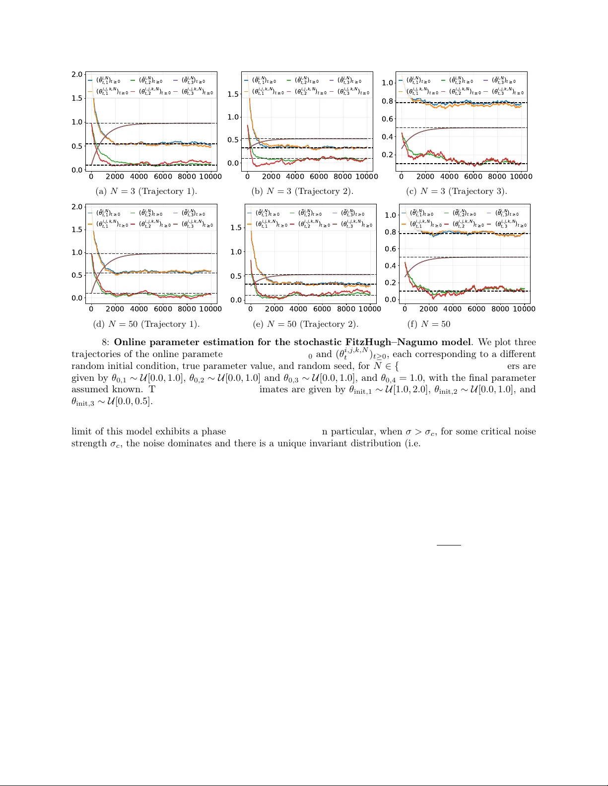
Eﬃcien t Online Learning in In teracting P article Systems Louis Sharro c k ∗ Nik olas Kantas † Grigorios A. P avliotis ‡ Abstract W e in tro duce a new metho d for online parameter estimation in sto chastic in teracting particle systems, based on contin uous observ ation of a small num b er of particles from the system. Our metho d recursively up dates the model parameters using a stochastic appro ximation of the gradien t of the asymptotic log- lik eliho o d, which is computed using the con tinuous stream of observ ations. Under suitable assumptions, w e rigorously establish conv ergence of our metho d to the stationary p oints of the asymptotic log-lik eliho o d of the interacting particle system. W e consider asymptotics b oth in the limit as the time horizon t → ∞ , for a ﬁxed and ﬁnite n um b er of particles, and in the join t limit as the n umber of particles N → ∞ and the time horizon t → ∞ . Under additional assumptions on the asymptotic log-likelihoo d, w e also establish an L 2 con vergence rate and a cen tral limit theorem. Finally , w e present sev eral n umerical examples of practical interest, including a mo del for systemic risk, a mo del of interacting FitzHugh–Nagumo neurons, and a Cuck er–Smale ﬂocking model. Our numerical results corroborate our theoretical results, and also suggest that our estimator is eﬀectiv e even in cases where the assumptions required for our theoretical analysis do not hold. 1 In tro duction The study of interacting particle systems (IPSs) and their mean-ﬁeld limits has a rich history , dating bac k to the seminal work of McKean [ 79 ] ; see [ 81 , 85 , 106 , 107 ] for some other early references. In the last t w o decades, the probabilistic properties of such systems hav e b een the sub ject of sustained in terest, with many new results on well-posedness [e.g., 29 , 55 ], existence and uniqueness [e.g., 7 , 59 , 83 ], ergo dicity [e.g., 6 , 15 , 24 , 26 , 43 ], and the propagation of chaos [e.g., 42 , 68 , 76 , 77 ]. In parallel, signiﬁcant attention has also b een dedicated to the v arious appli cations of such mo dels. These include, amongst others, statistical ph ysics [ 11 ], m ulti-agent systems [ 10 ], mean-ﬁeld games [ 20 , 21 , 22 ], sto c hastic control [ 17 ], ﬁltering [ 34 ], mathematical biology including neuroscience [ 5 ] and structured models of p opulation dynamics [ 18 ], the so cial sciences including opinion dynamics [ 30 , 51 ] and co op erativ e b ehaviours [ 19 ], ﬁnancial mathematics [ 49 ], Bay esian inference [ 72 ], and the analysis of mean-ﬁeld neural netw orks [ 54 , 80 , 92 , 103 ]. More recen tly , there has b een gro wing in terest in the study of statistical inference for this class of processes [e.g., 4 , 14 , 31 , 41 , 49 , 60 , 99 , 100 ], in b oth frequentist [e.g., 4 , 99 ] and Bay esian settings [e.g., 58 , 84 ]. One limitation of existing approaches is that, with certain notable exceptions [ 45 , 46 , 88 ], it is generally assumed that it is p ossible to observe the entire IPS, or else multiple i.i.d. tra jectories of the limiting McKean-Vlasov SDE (MVSDE). In cases where the n umber of particles is v ery large, how ever, this assumption may b e unrealistic, or else asso ciated with a prohibitive computational cost. In addition, most existing approaches are ‘oﬄine’ or ‘batch’ metho ds, which can b e impractical for large datasets where observ ations o ccur ov er a long time p eriod. In particular, existing metho ds typically rely on optimisation of a function (e.g., the log-likelihoo d) of the entire observed data path, whic h can b e impractically slo w for long time p erio ds, or for mo dels whic h are costly to ev aluate. One exception to this is [ 100 ], whic h in tro duced an eﬃcien t ‘online’ or ‘recursive’ estimator, and analysed its asymptotic prop erties. Unfortunately , the estimator in [ 100 ] still relies on observ ation of m ultiple i.i.d. paths of the MVSDE, or multiple tra jectories of the IPS. ∗ Department of Statistical Science, Univ ersity College London. l.sharrock@ucl.ac.uk † Department of Mathematics, Imp erial College London. n.kantas@imperial.ac.uk ‡ Department of Mathematics, Imp erial College London. g.pavliotis@imperial.ac.uk 1 In this context, a natural question is whether online parameter estimation in IPSs remains p ossible when only a single particle, or a small num ber of particles, can b e observed. In this pap er, we answ er this question in the aﬃrmative. 1.1 Con tributions Our main contributions are summarised b elow. Metho dology . W e deriv e a new online estimator for statistical inference in ergodic IPSs (and the asso ciated MVSDEs). Our estimator is based on minimising the asymptotic (b oth in time, and in the num b er of particles) negativ e log-likelihoo d of the IPS. It requires observ ation of the tra jectories of just three particles, whic h suﬃces to form an asymptotically unbiased estimate of the mean-ﬁeld interaction terms app earing in the gradien t of the asymptotic log-lik eliho o d. In comparison to existing online estimators, whic h assume it is p ossible to observe the tra jectory of every particle from the IPS, our estimator oﬀers signiﬁcan t computational adv antages in the typical case where N ≫ 1 . Theory . W e prov e, under suitable assumptions, that the prop osed estimator conv erges to the stationary p oin ts of the asymptotic log-likelihoo d of the IPS. Under additional assumptions on the asymptotic negative log-lik eliho o d (e.g., strong conv exit y), we show that our estimator is consisten t, in the sense that it conv erges in L 2 to the true parameter θ 0 , and obtain a central limit theorem. W e also presen t corresp onding guarantees for a comparable estimator which requires observ ation of all particles from the IPS, extending existing theoretical results. This enables a detailed comparison of the theoretical prop erties of b oth estimators. In all cases, we consider asymptotics in the case where the num b er of particles is ﬁxed and ﬁnite, and only the time horizon t → ∞ , and also in the case where b oth the n umber of particles N → ∞ and the time horizon t → ∞ . Applications. W e present extensiv e numerical results to demonstrate the p erformance of our estimator. Our n umerical results corrob orate our theoretical ﬁndings, and also suggest that our estimator is eﬀective in cases where our assumptions demonstrably do not hold, e.g., in situations where there exist multiple in v arian t measures, or the diﬀusion co eﬃcien t in the particle dynamics is degenerate. W e consider several mo dels of practical in terest, including a mo del for systemic risk, a mo del of interacting FitzHugh–Nagumo neurons, a Cuc ker–Smale ﬂo cking mo del, and a mean-ﬁeld 3 2 sto c hastic volatilit y mo del. 1.2 Related W ork P arameter Estimation in IPSs and MVSDEs. Until recent years, surprisingly little work had b een dev oted to the study of statistical inference for IPSs and MVSDEs. This is in stark con trast to the w ealth of literature on parameter estimation in linear SDEs, i.e., diﬀusion processes whose co eﬃcients do not dep end on the la w of the pro cess [e.g., 16 , 61 , 65 , 71 ]. A notable exception is the pioneering w ork of [ 60 ], who established asymptotic prop erties (consistency , asymptotic normalit y) of the maxim um likelihoo d estimator (MLE) for a system of weakly interacting particles in the limit as N → ∞ , based on contin uous observ ation of all N particles o ver a ﬁxed time interv al [0 , T ] . More recently , there has b een a surge of in terest in this topic. In particular, several authors ha ve extended the results in [ 60 ] in v arious directions [e.g., 4 , 14 , 31 , 41 , 49 , 99 , 100 ]. In particular, Bishw al [ 14 ] studied the case where only discrete observ ations of the system are av ailable, and the parameter to b e estimated is a function of time, while Gieseck e et al. [ 49 ] established asymptotic prop erties (consistency , asymptotic normalit y , asymptotic eﬃciency) of an approximate MLE for a muc h broader class of interacting sto chastic systems, widely applicable in ﬁnancial mathematics, which additionally allo w for discontin uous (i.e., jump) dynamics. Chen [ 31 ] established the optimal conv ergence rate for the MLE in an in teracting particle system with linear interaction in the limit as b oth N → ∞ and T → ∞ . Sharro c k et al. [ 99 ] established the asymptotic prop erties of the MLE in the limit as N → ∞ for a more general family of IPSs. Subsequently , Sharro c k et al. [ 100 ] in tro duced online (or recursive) MLEs for the parameters of an IPS or the asso ciated MVSDE, and analysed their asymptotic properties in the limit as T → ∞ , and the joint limit as T → ∞ and N → ∞ . [ 41 ] established the lo cal asymptotic normality of the MLE, and obtained simple and explicit criteria for identiﬁabilit y and non-degeneracy of the Fisher information matrix. Mean while, Amorino et al. [ 4 ] 2 studied join t parameter estimation for b oth the drift and diﬀusion co eﬃcients, based on discrete observ ations of the IPS ov er a ﬁxed time interv al [0 , T ] . In a rather diﬀeren t direction, Della Maestra and Hoﬀmann [ 40 ] ha ve considered non-parametric estimation of the drift term in a MVSDE, based on con tin uous observ ation of the asso ciated IPS ov er a ﬁxed time horizon. More sp eciﬁcally , the authors obtained adaptive estimators based on the solution map of the F okk er–Planck equation, and prov ed their optimality in a minimax sense. W e refer to [ 3 , 9 , 32 , 33 , 69 , 73 , 74 , 84 , 90 , 110 ] for other recent contributions on non-parametric (and semi-parametric) inference for IPSs. In most of the aforementioned works, statistical inference is based on direct observ ation of all N particles in the IPS, or observ ation of N i.i.d. tra jectories of the limiting MVSDE. In cases where the num ber of particles is very large, how ev er, this ma y b e unrealistic, or entail a prohibitive computational cost. In this con text, several authors hav e also studied estimation based on observ ation of a single particle from the IPS [ 88 , 89 , 90 ], or else a single tra jectory of the limiting MVSDE [ 33 , 45 , 46 ]. In particular, Genon-Catalot and Larédo [ 45 ] studied parametric inference for a sp eciﬁc class of one-dimensional MVSDEs with no p oten tial term and a p olynomial in teraction term, based on contin uous observ ation of a single sample path on the time in terv al [0 , 2 T ] in the stationary regime. Genon-Catalot and Larédo [ 46 ] considered a more general family of MVSDEs, and prop osed an alternativ e pseudo-likelihoo d approach based on a kernel estimator of the in v ariant density . Mean while, Pa vliotis and Zanoni [ 88 ] established the asymptotic prop erties (asymptotic un biasedness, asymptotic normality) of the eigenfunction martingale estimator as N → ∞ , based on discrete observ ations of a single tra jectory of the IPS on a ﬁxed time interv al [0 , T ] , while Pa vliotis and Zanoni [ 89 ] established consistency of the metho d of moments estimator as N → ∞ and T → ∞ . Finally , Pa vliotis and Zanoni [ 90 ] considered semi-parametric estimation of the in teraction kernel based on observ ation of a single particle using a generalised F ourier expansion. Online Parameter Estimation in Contin uous-Time Pro cesses. Ev en for linear SDEs, the literature on ‘online’ or ‘recursive’ parameter estimation is somewhat sparse, with some notable recent exceptions [ 13 , 95 , 96 , 98 , 102 , 104 , 105 ]. The problem of recursiv e estimation in con tinuous time sto c hastic pro cesses w as ﬁrst analysed by Gerencsér et al. [ 47 ] ; see also Gerencsér and Prok a j [ 48 ] , Lev anony et al. [ 70 ] for some other early references. More recen tly , this problem was revisited by Sirignano and Spiliop oulos [ 102 , 104 ] , who prop osed an online metho d—‘sto c hastic gradient descent in con tinuous time’—for statistical inference in fully observed diﬀusion pro cesses, and analysed its asymptotic prop erties (e.g., almost sure con vergence, asymptotic normalit y). Their metho d can b e seen as a form of contin uous-time sto c hastic gradient descent with respect to the asymptotic (or av erage) log-likelihoo d of the diﬀusion pro cess. This approach has since b een extended to partially observ ed diﬀusion pro cesses [ 97 , 98 , 105 ], jump diﬀusion pro cesses [ 13 ], nonlinear diﬀusion pro cesses [ 100 ], and sto chastic pro cesses driv en by coloured noise [ 87 ]. More recen tly , a related problem has also b een studied by W ang and Sirignano [ 108 , 109 ] . In particular, W ang and Sirignano [ 108 , 109 ] considered the task of minimising a function of the stationary distribution of a parameterised (linear, in the sense of McKean) diﬀusion pro cess. They in tro duced an eﬃcien t con tinuous-time sto c hastic gradient descent algorithm for this task, which con tinuously up dates the parameters of the mo del using an estimate for the gradient of the stationary distribution, which is simultaneously up dated using forw ard propagation of the deriv atives of the diﬀusion pro cess. They establish the conv ergence of their ‘online forw ard propagation algorithm’ to the stationary p oin ts of the ob jectiv e function for a broad class of diﬀusion pro cesses, and demonstrate its eﬃcacy in a num b er of applications. 1.3 P ap er Organisation The remainder of this pap er is organised as follows. In Section 2 , we introduce the problem of interest. In Section 3 , we present our main metho dological contributions. In Section 4 , we state our assumptions and our main theoretical results. In Section 5 , we present sev eral numerical examples illustrating our prop osed metho dology . Finally , in Section 6 , we provide some concluding remarks. Additional material, including pro ofs of our main results, is provided in the App endices. 3 2 Preliminaries 2.1 Notation W e use ⟨· , ·⟩ and ∥ · ∥ to denote, respectively , the Euclidean inner product and the Euclidean norm on R d . F or matrices and higher order tensors, we use ∥ · ∥ to denote the F robenius norm. Finally , we write ∥ · ∥ p to denote the ℓ p norm. W e write P ( R d ) for the collection of all probability measures on R d and P p ( R d ) = { µ ∈ P ( R d ) : R R d ∥ x ∥ p µ (d x ) < ∞} for the collection of all probability measures on R d with ﬁnite p th momen t. In a sligh t abuse of notation, w e will o ccasionally write µ ( ∥ · ∥ p ) = R R d ∥ x ∥ p µ (d x ) for the p th momen t of µ . F or p ≥ 1 , and µ, ν ∈ P p ( R d ) , we will write W p ( µ, ν ) to denote the W asserstein distance b et ween µ and ν , viz. W p ( µ, ν ) = inf π ∈ Π( µ,ν )  Z R d × R d ∥ x − y ∥ p π (d x, d y )  1 p , where Π( µ, ν ) d enotes the set of all couplings of µ and ν . That is, the set of all probability measures on R d × R d with marginals µ and ν . 2.2 The Mo del W e consider a weakly interacting particle system (IPS) on R d , parameterised by θ ∈ Θ , of the form d x θ,i,N t =  − ∇ V ( θ, x θ,i,N t ) − 1 N N X j =1 ∇ W ( θ , x θ,i,N t − x θ,j,N t )  d t + σ d w i,N t , t ≥ 0 , (1) where V ( θ , · ) : R d → R , W ( θ , · ) : R d → R are contin uously diﬀerentiable functions, σ ∈ R d × d is a constant, in vertible matrix, w i,N := ( w i,N t ) t ≥ 0 are a set of indep endent R d -v alued standard Brownian motions, and Θ ⊆ R p is an open set. W e assume that ( x i,N 0 ) N i =1 are a set of i.i.d. R d -v alued random v ariables, with common la w µ 0 , indep endent of ( w i,N t ) t ≥ 0 . W e will commonly refer to V as the c onﬁnement p otential , and to W as the inter action p otential . F or notational conv enience, it will also b e useful for us to introduce the drift function b : R p × R d × R d → R d , deﬁned according to b ( θ , x, y ) := −∇ V ( θ , x ) − ∇ W ( θ , x − y ) . Using this notation, the IPS can b e written as d x θ,i,N t = h 1 N N X j =1 b ( θ , x θ,i,N t , x θ,j,N t ) i d t + σ d w i,N t . (2) W e will assume, throughout this pap er, that there exists a true, static parameter θ 0 ∈ Θ which generates observ ations ( x i,N t ) t ≥ 0 := ( x θ 0 ,i,N t ) t ≥ 0 of the IPS ( 1 ) . Thus, we op erate under the exact mo delling regime, and in our notation will suppress the dep endence of the observed path on the true parameter θ 0 . Remark 1. It wil l sometimes b e useful to view the IPS in ( 1 ) as an SDE on ( R d ) N . In p articular, supp ose we write x θ,N t = ( x θ, 1 ,N t , . . . , x θ,N ,N t ) ⊤ ∈ ( R d ) N . Then this pr o c ess is the solution of d x θ,N t = B N ( θ , x θ,N t )d t + Σ N d w N t , (3) wher e Σ N = I N ⊗ σ , w N = ( w 1 ,N , . . . , w N ,N ) ⊤ is a ( R d ) N -value d standar d Br ownian motion, and the function B N ( θ , · ) : ( R d ) N → ( R d ) N is deﬁne d ac c or ding to the form B N ( θ , x N ) = ( B i,N ( θ , x N ) , . . . , B N ,N ( θ , x N )) ⊤ , wher e, for e ach i ∈ [ N ] := { 1 , . . . , N } , the function B i,N ( θ , · ) : ( R d ) N → R d is deﬁne d ac c or ding to B i,N ( θ , x N ) = 1 N P N j =1 b ( θ , x i,N , x j,N ) . 2.3 The Mean-Field Mo del W e are interested in the regime where the num b er of particles N ≫ 1 so that, under app ropriate conditions whic h we will later imp ose [e.g., 26 , 76 ], an y single particle in the IPS can b e well approximated by the solution of the limiting MVSDE, viz. d x θ t =  − ∇ V ( θ, x θ t ) − Z R d ∇ W ( θ , x θ t − y ) µ θ t (d y )  d t + σ d w t , t ≥ 0 , (4) 4 where w = ( w t ) t ≥ 0 is a standard R d -v alued Brownian motion, and µ θ t = L ( x θ t ) denotes the law of x θ t . This phenomenon is known as the pr op agation of chaos [ 27 , 28 , 106 ]. 2.4 Mo del Assumptions W e are no w ready to state some initial assumptions on the data generating pro cess. W e b egin with the follo wing integrabilit y assumption on the initial condition. Assumption 2. The initial law satisﬁes µ 0 ∈ P k ( R d ) for al l k ∈ N . Mean while, regarding the true drift function, i.e., the drift function ev aluated at the true parameter, we imp ose one of the following tw o sets of assumptions. Assumption 3. The functions x 7→ V ( θ 0 , x ) and x 7→ W ( θ 0 , x ) ar e twic e c ontinuously diﬀer entiable. In addition, they satisfy one of the fol lowing two c onditions: (a)(i) V ( θ 0 , · ) satisﬁes the C ( A, α ) c ondition. That is, ther e exist A > 0 , α ≥ 0 such that, for al l 0 < ε < 1 , and for al l x, y ∈ R d , ( x − y ) · ( ∇ V ( θ 0 , x ) − ∇ V ( θ 0 , y )) ≥ Aε α  ∥ x − y ∥ 2 − ε 2  . In addition, ∇ V ( θ 0 , · ) is lo c al ly Lipschitz with p olynomial gr owth, and ∇ 2 V ( θ 0 , · ) has p olynomial gr owth. That is, ther e exist C , m > 0 such that, for al l x, y ∈ R d , ∥∇ V ( θ 0 , x ) − ∇ V ( θ 0 , y ) ∥ ≤ C ∥ x − y ∥ (1 + ∥ x ∥ m + ∥ y ∥ m ) , ∥∇ 2 V ( θ 0 , x ) ∥ ≤ C (1 + ∥ x ∥ m ) . (a)(ii) W ( θ 0 , · ) is symmetric and c onvex, ∇ W ( θ 0 , · ) is lo c al ly Lipschitz with p olynomial gr owth, and ∇ 2 W ( θ 0 , · ) has p olynomial gr owth. That is, ther e exist C, m > 0 such that, for al l x, y ∈ R d , ∥∇ W ( θ 0 , x ) − ∇ W ( θ 0 , y ) ∥ ≤ C ∥ x − y ∥ (1 + ∥ x ∥ m + ∥ y ∥ m ) , ∥∇ 2 W ( θ 0 , x ) ∥ ≤ C (1 + ∥ x ∥ m ) . or (b)(i) V ( θ 0 , · ) = 0 . (b)(ii) W ( θ 0 , · ) is symmetric, ∇ W ( θ 0 , · ) is lo c al ly Lipschitz with p olynomial gr owth, and ∇ 2 W ( θ 0 , · ) has p olynomial gr owth. That is, ther e exist C , m > 0 such that, for al l x, y ∈ R d , ∥∇ W ( θ 0 , x ) − ∇ W ( θ 0 , y ) ∥ ≤ C ∥ x − y ∥ (1 + ∥ x ∥ m + ∥ y ∥ m ) , ∥∇ 2 W ( θ 0 , x ) ∥ ≤ C (1 + ∥ x ∥ m ) . In addition, W ( θ 0 , · ) satisﬁes the C ( A, α ) c ondition. That is, ther e exist A > 0 , α ≥ 0 , such that, for al l 0 < ε < 1 , and for al l x, y ∈ R d , ( x − y ) · ( ∇ W ( θ 0 , x ) − ∇ W ( θ 0 , y )) ≥ Aε α  ∥ x − y ∥ 2 − ε 2  . These conditions ensure the existence and uniqueness of a strong solution to the (observ ed) IPS and the asso ciated MVSDE [ 26 , Theorem 2.6], uniform-in-time momen t b ounds [ 26 , Prop osition 2.7], uniform-in-time propagation of chaos [ 26 , Theorem 3.1], and the existence of, and con vergence to, a unique in v ariant measure [ 26 , Theorem 4.1]. 1 , 2 W e provide a precise statement of these results in App endix A . 1 Under Assumption 3 (b), the required results in fact hold for a pro jected or centered version of the observ ed IPS, deﬁned b y y i,N t = x i,N t − 1 N P N j =1 x j,N t [ 26 , Section 2]. This still deﬁnes a diﬀusion process, but no w on the hyperplane M N = { x N ∈ ( R d ) N : P N i =1 x i,N = 0 } . F or notational conv enience, in the remainder we will state all results using the notation ( x i,N t ) i ∈ [ N ] t ≥ 0 , with this understo od to mean the centered pro cess ( y i,N t ) i ∈ [ N ] t ≥ 0 when Assumption 3 (b) holds. 2 Under Assumption 3 (b), the MVSDE in fact admits a one-parameter family of inv ariant distributions, the parameter corresponding to the mean of the inv ariant distribution. Th us, the inv ariant distribution is unique once its expectation has b een speciﬁed. Throughout this pap er, we will assume that the mean is ﬁxed, and without loss of generalit y set it to zero [see, e.g., 26 ]. 5 Remark 4. Mor e gener al ly, our the or etic al analysis r emains valid under any c onditions which guar ante e uniform-in-time moment b ounds, uniform-in-time pr op agation of chaos, and c onver genc e (at a suﬃciently fast r ate) to an invariant me asur e. Se e, e.g., [ 76 , 77 ] for some classic al assumptions, and [ 23 , 39 , 66 , 67 , 68 ] for some mor e r e c ent r esults. W e cho ose to adopt the c onditions intr o duc e d in Cattiaux et al. [ 26 ] as they ar e at onc e suﬃciently gener al to hold for many mo dels of pr actic al inter est (se e Se ction 5 ), whilst not b eing so gener al as to demand a signiﬁc ant additional notational overhe ad. Finally , we will imp ose the follo wing regularit y assumptions on the conﬁnemen t p otential and the in teraction p otential. Assumption 5. F or al l θ ∈ Θ , the functions x 7→ ∇ V ( θ , x ) and x 7→ ∇ W ( θ , x ) ar e c ontinuously diﬀer entiable. F or al l x ∈ R d , the functions θ 7→ ∇ V ( θ , x ) and θ 7→ ∇ W ( θ , x ) ar e thr e e times c ontinuously diﬀer entiable. In addition, for k = 0 , 1 , 2 , 3 : (i) Ther e exist C k , m k > 0 such that, for al l θ ∈ Θ , and for al l x, y ∈ R d , ∥ ∂ k θ ∇ V ( θ , x ) − ∂ k θ ∇ V ( θ , y ) ∥ ≤ C k ∥ x − y ∥  1 + ∥ x ∥ m k + ∥ y ∥ m k  ∥ ∂ k θ ∇ V ( θ , 0) ∥ ≤ C k (ii) Ther e exist C k , m k > 0 such that, for al l θ ∈ Θ , and for al l x, y ∈ R d , ∥ ∂ k θ ∇ W ( θ , x ) − ∂ k θ ∇ W ( θ , y ) ∥ ≤ C k ∥ x − y ∥  1 + ∥ x ∥ m k + ∥ y ∥ m k  ∥ ∂ k θ ∇ W ( θ , 0) ∥ ≤ C k Remark 6. In the c ase wher e Θ ⊂ R p , these assumptions ar e very mild, and wil l hold for essential ly al l of the mo dels that we enc ounter in pr actic e. On the other hand, when Θ = R p , they ar e somewhat r estrictive. Given this, it is worth noting that it is p ossible to establish our r esults under we aker assumptions, which additional ly al low for x 7→ ∇ V ( θ, x ) and x 7→ ∇ W ( θ , x ) to gr ow line arly in ∥ θ ∥ [se e, e.g., 104 ]. 2.5 The Lik eliho o d F unction W e are interested in online inference for the unknown parameter θ 0 . W e will p erform this task based on recursiv e maximisation of an appropriate likelihoo d function. 2.5.1 The Log-Lik eliho o d of the Interacting P article System Let P θ,N t denote the probability measure induced by the tra jectories ( x θ,i,N s ) i ∈ [ N ] s ∈ [0 ,t ] of the IPS. Then, using Girsano v’s Theorem [e.g., 86 ], we hav e a log-likelihoo d function given (up to an additive constant) by [e.g., 41 , 60 ] L N t ( θ ) = Z t 0 ⟨ B N ( θ , x N s ) , (Σ N Σ ⊤ N ) − 1 d x N s ⟩ − 1 2 Z t 0 ∥ B N ( θ , x N s ) ∥ 2 Σ N Σ ⊤ N d s (5) = N X i =1 h Z t 0  B i,N ( θ , x N s ) , ( σ σ ⊤ ) − 1 d x i,N s  − 1 2 Z t 0 ∥ B i,N ( θ , x N s ) ∥ 2 σ σ ⊤ d s i (6) = N X i =1 h Z t 0  B ( θ , x i,N s , µ N s ) , ( σ σ ⊤ ) − 1 d x i,N s  − 1 2 Z t 0 ∥ B ( θ , x i,N s , µ N s ) ∥ 2 σ σ ⊤ d s i (7) where µ N s = 1 N P N j =1 δ x j,N s denotes the empirical la w of the observed IPS, B ( θ , x, µ ) = R b ( θ , x, y ) µ (d y ) , and ∥ z ∥ 2 σ σ ⊤ := ⟨ z , z ⟩ σ σ ⊤ := ⟨ z , ( σ σ ⊤ ) − 1 z ⟩ . 3 , 4 3 Strictly sp eaking, to use Girsanov’s theorem to deﬁne the log-lik eliho o d in ( 5 ) we m ust assume that, for all θ ∈ Θ , the likelihood ratio pro cess Z θ s := d P θ,N t / d W N t   F s , s ∈ [0 , t ] exists and is a martingale under W N t , the unique law (on path space) of the driftless system d x N s = Σ N d w N s , with the same initial condition as the original pro cess. In the absence of this assumption, we can simply view the function in ( 5 ) as a con trast function, and proceed in the same wa y . 4 Under Assumption 3 (b), w e must consider the log-likelihood asso ciated with the centered pro cess ( y θ,i,N s ) i ∈ [ N ] s ∈ [0 ,t ] . This requires additional care, since the diﬀusion co eﬃcient ˜ Σ N is no w singular on ( R d ) N . Nonetheless, with the addition of a small addendum to Assumption 3 (b), one can sho w that the log-lik elihoo d for the cen tered IPS takes precisely the same functional form as for the non-cen tered IPS. Thus, our subsequent metho dological dev elopmen ts are applicable in this case. W e discuss this further in App endix B . 6 W e are ﬁrst interested in the asymptotic b ehaviour of this function as the time horizon t → ∞ , for a ﬁxed and ﬁnite num b er of particles N ∈ N . This is the sub ject of the following prop osition. Prop osition 7. Supp ose that Assumption 2 , Assumption 3 , and Assumption 5 (with k = 0 ) hold. Then, as t → ∞ , it holds that 1 t [ L N t ( θ ) − L N t ( θ 0 )] a . s . − − → L 1 − 1 2 Z ( R d ) N h N X i =1     B i,N ( θ , x N ) − B i,N ( θ 0 , x N )     2 σ σ ⊤ i π N θ 0 (d x N ) . (8) wher e π N θ 0 ∈ P (( R d ) N ) denotes the unique invariant me asur e of the IPS evaluate d at the true p ar ameter θ 0 . Pr o of. See App endix C.1.1 . Mean while, the asymptotic behaviour of these functions as the num b er of particles N → ∞ , for a ﬁxed and ﬁnite time horizon t ∈ R + , is established in the following prop osition. Prop osition 8. Supp ose that Assumption 2 , Assumption 3 , and Assumption 5 (with k = 0 ) hold. Then, as N → ∞ , it holds that 1 N  L N t ( θ ) − L N t ( θ 0 )  L 1 − → − 1 2 Z t 0  Z R d ∥ B ( θ , x, µ θ 0 s ) − B ( θ 0 , x, µ θ 0 s ) ∥ 2 σ σ ⊤ µ θ 0 s (d x )  d s (9) wher e µ θ 0 s = La w ( x θ 0 s ) ∈ P ( R d ) denotes the law of the MVSDE evaluate d at the true p ar ameter θ 0 . Pr o of. See App endix C.1.1 . Finally , we can characterise the b ehaviour of the log-likelihoo d of the IPS in the joint limit as N → ∞ and t → ∞ . Corollary 9. Supp ose that Assumption 2 , Assumption 3 , and Assumption 5 (with k = 0 ) hold. Then, as N → ∞ and then t → ∞ , it holds that 1 N t  L N t ( θ ) − L N t ( θ 0 )  L 1 − → − 1 2 Z R d ∥ B ( θ , x, π θ 0 ) − B ( θ 0 , x, π θ 0 ) ∥ 2 σ σ ⊤ π θ 0 (d x ) (10) wher e π θ 0 ∈ P ( R d ) denotes the unique invariant me asur e of the MVSDE evaluate d at the true p ar ameter θ 0 . Pr o of. See App endix C.1.1 2.5.2 The Log-Lik eliho o d of the McKean–Vlasov SDE Let P θ t denote the probability measure induced by the solution ( x θ s ) s ∈ [0 ,t ] of the MVSDE ( 4 ) . Then, once more app ealing to Girsanov’s Theorem, we hav e a log-lik eliho o d function giv en by [e.g., 41 , Section 2.3] L t ( θ ) = Z t 0  B ( θ , x s , µ θ s ) , ( σ σ ⊤ ) − 1 d x s  − 1 2 Z t 0   B ( θ , x s , µ θ s )   2 σ σ ⊤ d s (11) where ( x s ) s ≥ 0 := ( x θ 0 s ) s ≥ 0 denotes the path of the MVSDE at the true parameter θ 0 . In this case, we are just interested in the asymptotic b ehaviour of this function as the time horizon t → ∞ . In particular, w e ha ve the following result. Prop osition 10. Supp ose that Assumption 2 , Assumption 3 , and Assumption 5 (with k = 0 ) hold. 5 Then, as t → ∞ , it holds that 1 t [ L t ( θ ) − L t ( θ 0 )] L 1 − → − 1 2 Z R d ∥ B ( θ , x, π θ ) − B ( θ 0 , x, π θ 0 ) ∥ 2 σ σ ⊤ π θ 0 (d x ) . (12) wher e π θ , π θ 0 ∈ P ( R d ) denote the unique invariant me asur es of the MVSDE, evaluate d at the p ar ameter θ and the true p ar ameter θ 0 , r esp e ctively. 5 F or this result, w e in fact require that Assumption 3 holds for all θ ∈ Θ , and not just for θ = θ 0 . This ensures the existence of the family of inv ariant measures ( π θ ) θ ∈ Θ . 7 Pr o of. See App endix C.1.2 . Remark 11. Curiously, the asymptotic lo g-likeliho o d of the IPS in the joint limit as N → ∞ and t → ∞ , c.f. ( 10 ) , do es not c oincide with the asymptotic lo g-likeliho o d of the MVSDE as t → ∞ , c.f. ( 12 ) . This b eing said, the two functions do c oincide (and ar e b oth maximise d) at the true p ar ameter θ 0 . This disp arity is p erhaps a little surprising. Inde e d, under the assumption of uniform-in-time pr op agation of chaos, we know that the dynamics of the IPS wil l c onver ge to the dynamics of the McKe an–Vlasov pr o c ess as N → ∞ and t → ∞ . The discr ep ancy arises b e c ause the lo g-likeliho o d of the IPS uses the empiric al distribution of the observe d system µ N t , which c onver ges to π θ 0 , while the lo g-likeliho o d of the MVSDE uses the mo del distribution µ θ t , which c onver ges to π θ . 3 Metho dology Our goal is to recursively estimate the true parameter θ 0 in real time, using the contin uous stream of observ ations of a (subset of ) the full collection of particles ( x i,N t ) i ∈ [ N ] t ≥ 0 from the IPS. 6 T o achiev e this task, w e will seek to recursively minimise an appropriately chosen ob jectiv e. 3.1 The Ob jectiv e F unction W e are interested in the case where the n umber of particles N ≫ 1 , and thus any single particle in the IPS ( 1 ) resem bles a solution of the MVSDE ( 4 ) . In this regime, there are t wo natural c hoices for the ob jective function. The ﬁrst is the a verage ne gative log-likelihoo d of the IPS, whic h under the conditions sp eciﬁed in Corollary 9 is giv en by: L ( θ ) := Z R d 1 2 ∥ B ( θ , x, π θ 0 ) − B ( θ 0 , x, π θ 0 ) ∥ 2 σ σ ⊤ π θ 0 (d x ) := Z R d L ( θ , x, π θ 0 ) π θ 0 (d x ) . (13) The second is the av erage negative log-likelihoo d of the limiting MVSDE, which under the conditions sp eciﬁed in Prop osition 10 is given by: J ( θ ) := Z R d 1 2 ∥ B ( θ , x, π θ ) − B ( θ 0 , x, π θ 0 ) ∥ 2 σ σ ⊤ π θ 0 (d x ) := Z R d J ( θ , x, π θ , π θ 0 ) π θ 0 (d x ) . (14) Remark 12. These two functions ar e non-ne gative for al l θ ∈ Θ and, under standar d identiﬁability assumptions [e.g., 45 , Assumptions S2,S4], uniquely minimise d (and e qual to zer o) at the true p ar ameter θ 0 . In terestingly , designing recursive maximum lik eliho o d estimators with resp ect to the tw o ob jective functions in ( 13 ) , ( 14 ) will lead to rather diﬀerent algorithms. In this pap er, w e will fo cus exclusively on algorithms designed with reference to the ﬁrst ob jectiv e function. The second will b e the sub ject of a forthcoming pap er [ 101 ]. 3.2 Gradien t Descen t in Con tinuous Time In order to optimise the ob jectiv e function in ( 13 ) , a natural approach is to simulate the corresp onding gr adient ﬂow , or curve of ste ep est desc ent . Let θ init ∈ Θ . Then, the gradien t ﬂow ( θ t ) t ≥ 0 of L is deﬁned as the solution of d θ t = − γ t ∂ θ L ( θ t )d t, (15) where γ t : R + → R + is a deterministic, p ositiv e, non-increasing function commonly referred to as the le arning r ate . Thus, for all t ≥ 0 , ( θ t ) t ≥ 0 follo ws the direction of steep est descent with resp ect to the asymptotic log-lik eliho o d function of the IPS. 6 In the case where Assumption 3 (b) holds (i.e., the conﬁnemen t potential is n ull), w e m ust assume it is p ossible to observ e (a subset of ) the center ed particles ( y i,N t ) i ∈ [ N ] t ≥ 0 . This ensures that the results required for our theoretical analysis (e.g., propagation-of-chaos, conv ergence to a unique inv ariant measure) con tinue to hold (see Remark 1 ). 8 Remark 13. The deﬁnition of the gr adient ﬂow ab ove diﬀers slightly fr om the standar d deﬁnition of a gr adient ﬂow [e.g., 94 ], due to the additional inclusion of the le arning r ate ( γ t ) t ≥ 0 . Given this, we wil l sometimes inste ad r efer to ( 15 ) as “gr adient desc ent in c ontinuous time”, in line with the taxonomy intr o duc e d in [ 102 ]. W e c an r e c over the standar d deﬁnition of the gr adient ﬂow after a time r ep ar ameterisation. In p articular, deﬁning a new time c o or dinate as τ = τ ( t ) = R t 0 γ s d s , we have d θ τ = − ∂ θ L ( θ τ )d τ . Remark 14. In or der to ac c ount for the c ase wher e Θ ⊊ R p , we shal l in fact use a mo diﬁe d version of this e quation [e.g., 105 ], setting d θ t =  − γ t ∂ θ L ( θ t )d t , θ t ∈ Θ , 0 , θ t / ∈ Θ . (16) F or notational c onvenienc e, in what fol lows we wil l always write up date e quations in the form ( 15 ) . However, this should always b e understo o d to me an ( 16 ) . 3.2.1 The Gradien t of the Asymptotic Log-Likelihoo d F unctions In order to implement the gradient ﬂow in ( 15 ) w e will ﬁrst need to compute the gradient of the ob jective function. This is the sub ject of the following prop osition. Prop osition 15. Supp ose that Assumption 2 , Assumption 3 , and Assumption 5 (with k = 0 , 1 ) hold. Then the gr adient of the ne gative asymptotic lo g-likeliho o d function L with r esp e ct to θ is given by 7 ∂ θ L ( θ ) = Z R d H ( θ , x, π θ 0 ) π θ 0 (d x ) (17) wher e H : R p × R d × P ( R d ) → R p × 1 is given by H ( θ , x, µ ) := G ( θ , x, µ )( σ σ ⊤ ) − 1 ( B ( θ , x, µ ) − B ( θ 0 , x, µ )) , and G : R p × R d × P ( R d ) → R p × d is given by G ( θ , x, µ ) := ∂ θ B ( θ , x, µ ) = Z R d ∂ θ b ( θ , x, y ) µ (d y ) . Pr o of. See App endix C.2 . 3.3 Sto c hastic Gradien t Descen t in Contin uous Time In practice, we cannot simulate the gradient ﬂow in ( 15 ) directly , ev en after a suitable time-discretisation. In particular, it is not p ossible to compute ∂ θ L , since this gradient is given b y an exp ectation with resp ect to the unkno wn inv ariant measure π θ 0 . T o pro ceed, we th us seek a sto c hastic estimate for ∂ θ L . Ideally , we would lik e to b e able to compute this estimate in an online fashion, based on the contin uous stream of observ ations. 3.3.1 A Sto c hastic Estimate of the Gradien t of the Asymptotic Log-Likelihoo d Belo w, we provide a formal deriv ation of one such estimate; the use of this estimate will later b e justiﬁed rigorously . W e begin with the observ ation that, due to ergo dicit y and the con v ergence of µ θ 0 s → π θ 0 as s → ∞ , it holds that ∂ θ L ( θ ) L 1 = lim t →∞ 1 t  Z t 0 G ( θ , x i s , µ θ 0 s )( σ σ ⊤ ) − 1  B ( θ , x i s , µ θ 0 s ) − B ( θ 0 , x i s , µ θ 0 s )  d s  . 7 Here, and in the remainder, we use the conv en tion that the gradient op erator ∂ θ adds a con trav ariant dimension to the tensor ﬁeld on whic h it acts. Thus, for example, ∂ θ L ( θ ) is a column vector, taking v alues in R p × 1 . Meanwhile, G ( θ, x, µ ) := ∂ θ B ( θ, x, µ ) is a matrix, taking v alues in R p × d . 9 where ( x i s ) s ≥ 0 is a solution of the MVSDE in ( 4 ) , driven by the same Brownian motion and with the same initial conditions as the solution ( x i,N s ) s ≥ 0 of the IPS in ( 1 ) . Substituting B ( θ 0 , x i s , µ θ 0 s )d s = d x i s − σ d w i s from ( 4 ) , and noting that the additional martingale term conv erges to zero b oth a.s. and in L 1 under our conditions, it follows that ∂ θ L ( θ ) L 1 = lim t →∞ 1 t  Z t 0 G ( θ , x i s , µ θ 0 s )( σ σ ⊤ ) − 1  B ( θ , x i s , µ θ 0 s )d s − d x i s   Finally , due to uniform-in-time propagation of chaos, which guarantees that µ N s → µ θ 0 s and x i,N s → x i s in L 2 (and hence L 1 ) as N → ∞ , for all s ≥ 0 , w e hav e ∂ θ L ( θ ) L 1 = lim t →∞ lim N →∞ 1 t  Z t 0 G ( θ , x i,N s , µ N s )( σ σ ⊤ ) − 1  B ( θ , x i,N s , µ N s )d s − d x i,N s   This expression suggests that, when the num b er of particles N ≫ 1 , a natural stochastic estimate for ∂ θ L ( θ t )d t is giv en by ∂ θ L ( θ t )d t ≈ G ( θ t , x i,N t , µ N t )( σ σ ⊤ ) − 1  B ( θ t , x i,N t , µ N t )d t − d x i,N t  3.3.2 The Algorithm Substituting this expression into ( 15 ), we obtain our ﬁrst algorithm for optimising the ob jectiv e function L . Let ¯ θ i,N init ∈ Θ . Then, for t ≥ 0 , up date d ¯ θ i,N t = − γ t G ( ¯ θ i,N t , x i,N t , µ N t )( σ σ ⊤ ) − 1  B ( ¯ θ i,N t , x i,N t , µ N t )d t − d x i,N t  , (18) It is instructiv e to rewrite the up date equation in ( 18 ) in a di ﬀeren t form, which emphasises the connection with the ob jective function L . In particular, after substituting the particle dynamics from ( 1 ) , and performing some simple algebraic manipulations, we can rewrite ( 18 ) as d ¯ θ i,N t = − γ t G ( ¯ θ i,N t , x i,N t , µ N t )( σ σ ⊤ ) − 1  B ( ¯ θ i,N t , x i,N t , µ N t ) − B ( θ 0 , x i,N t , µ N t )  d t − σ d w i,N t  = − γ t H ( ¯ θ i,N t , x i,N t , µ N t )d t | {z } noisy descent term + γ t G ( ¯ θ i,N t , x i,N t , µ N t ) σ −⊤ d w i,N t | {z } noise term , = − γ t ∂ θ L ( ¯ θ i,N t )d t | {z } true descent term − γ t ( H ( ¯ θ i,N t , x i,N t , µ N t ) − ∂ θ L ( ¯ θ i,N t ))d t | {z } ﬂuctuations term + γ t G ( ¯ θ i,N t , x i,N t , µ N t ) σ −⊤ d w i,N t | {z } noise term . Remark 16. The estimator ( ¯ θ i,N t ) t ≥ 0 deﬁne d in ( 18 ) c oincides with one of the estimators pr op ose d in [ 100 ]. The obvious disadvantage of this estimator is that it r e quir es observation of the ful l system ( x i,N t ) i ∈ [ N ] t ≥ 0 of inter acting p articles, via the empiric al law µ N t = 1 N P N j =1 δ x j,N t . In c ases wher e the numb er of p articles N is very lar ge, ( ¯ θ i,N t ) t ≥ 0 may ther efor e b e pr ohibitively exp ensive to implement. 3.4 Sto c hastic Gradien t Descen t in Contin uous Time: A New Approach W e now seek an alternative estimator which do es not require observ ation of the entire se t of interacting particles. 3.4.1 A New Expression for the Gradients of the Asymptotic Log-Likelihoo d In order to obtain such an estimator, we will ﬁrst obtain an alternative form for the asymptotic log-likelihoo d and its gradients. W e b egin b y expanding the in tegrand in our existing expressions for the asymptotic negativ e log-likelihoo d function in ( 13 ), whic h yields L ( θ ) = Z R d 1 2 ∥ B ( θ , x, π θ 0 ) − B ( θ 0 , x, π θ 0 ) ∥ 2 σ σ ⊤ π θ 0 (d x ) = Z ( R d ) 3 1 2  b ( θ , x, y ) − B ( θ 0 , x, π θ 0 ) , b ( θ , x, z ) − B ( θ 0 , x, π θ 0 )  σ σ ⊤ π ⊗ 3 θ 0 (d x, d y , d z ) := Z ( R d ) 3 ℓ ( θ , x, y , z , π θ 0 ) π ⊗ 3 θ 0 (d x, d y , d z ) . 10 Similarly , expanding the integrand in our existing expression for the gradien t of the asymptotic negative log-lik eliho o d function in ( 17 ), it is p ossible to show that ∂ θ L ( θ ) = Z R d  G ( θ , x, π θ 0 )  ( σ σ ⊤ ) − 1  B ( θ , x, π θ 0 ) − B ( θ 0 , x, π θ 0 )  π θ 0 (d x ) = Z ( R d ) 3  g ( θ , x, y )  ( σ σ ⊤ ) − 1  b ( θ , x, z ) − B ( θ 0 , x, π θ 0 )  π ⊗ 3 θ 0 (d x, d y , d z ) := Z ( R d ) 3 h ( θ , x, y , z , π θ 0 ) π ⊗ 3 θ 0 (d x, d y , d z ) , where, in the second line, we hav e deﬁned g ( θ , x, y ) := ∂ θ b ( θ , x, y ) . This alternative represen tation of the gradien t of the asymptotic negative log-likelihoo d will pro vide the starting p oint for our new, more eﬃcien t sto c hastic estimate. 3.4.2 A New Sto chastic Estimate of the Gradien t of the Asymptotic Log-Likelihoo d Once again, w e present a formal deriv ation, deferring a rigorous theoretical treatment to the sequel. Similar to b efore, due to ergo dicity and the conv ergence of µ θ 0 s → π θ 0 as s → ∞ , we hav e that ∂ θ L ( θ ) L 1 = lim t →∞ 1 t h Z t 0 h g ( θ , x i s , x j s ) i ( σ σ ⊤ ) − 1 h b ( θ , x i s , x k s ) − B ( θ 0 , x i s , µ θ 0 s ) i d s i , where ( x i s ) s ≥ 0 , ( x j s ) s ≥ 0 , ( x k s ) s ≥ 0 are three indep enden t solutions of the MVSDE, driv en by Brownian motions ( w i s ) s ≥ 0 , ( w j s ) s ≥ 0 , ( w k s ) s ≥ 0 . Substituting B ( θ 0 , x i s , µ θ 0 s )d s = d x i s − σ d w i s , and using the fact that the additional martingale term conv erges to zero, we hav e that ∂ θ L ( θ ) L 1 = lim t →∞ 1 t h Z t 0  g ( θ , x i s , x j s )  ( σ σ ⊤ ) − 1  b ( θ , x i s , x k s )d s − d x i s  i Finally , under the assumption of uniform-in-time propagation of chaos, it follows from the previous display that ∂ θ L ( θ ) L 1 = lim t →∞ lim N →∞ 1 t h Z t 0  g ( θ , x i,N s , x j,N s )  ( σ σ ⊤ ) − 1  b ( θ , x i,N s , x k,N s )d s − d x i,N s  i where ( x i,N s ) s ≥ 0 , ( x j,N s ) s ≥ 0 , and ( x k,N s ) s ≥ 0 are the tra jectories of three distinct particles from the observed IPS. This expression suggests that, for N ≫ 1 , an alternative sto c hastic estimate for ∂ θ L ( θ t )d t is given by ∂ θ L ( θ t )d t ≈  g ( θ t , x i,N t , x j,N t )  ( σ σ ⊤ ) − 1  b ( θ t , x i,N t , x k,N t )d t − d x i,N t  . 3.4.3 A New Algorithm Substituting this expression into ( 15 ) , w e obtain an alternativ e algorithm for optimising the ob jective function L . Let θ i,j,k,N init ∈ Θ . Then, for t ≥ 0 , evolv e d θ i,j,k,N t = − γ t  g ( θ i,j,k,N t , x i,N t , x j,N t )  ( σ σ ⊤ ) − 1  b ( θ i,j,k,N t , x i,N t , x k,N t )d t − d x i,N t  . (19) Once again, it is instructive to rewrite this algorithm in a slightly diﬀeren t form. In this case, following similar manipulations to b efore, we hav e that d θ i,j,k,N t = − γ t ∂ θ L ( θ i,j,k,N t )d t | {z } true descent term − γ t ( h ( θ i,j,k,N t , x i,N t , x j,N t , x k,N t , µ N t ) − ∂ θ L ( θ i,j,k,N t ))d t | {z } ﬂuctuations term + γ t g ( θ i,j,k,N t , x i,N t , x j,N t ) σ −⊤ d w i,N t | {z } noise term . 11 Remark 17. In some sense, one c an view the estimator ( ¯ θ i,N t ) t ≥ 0 fr om Se ction 3.3.2 , as deﬁne d in ( 18 ) , as an “aver age d” version of our new estimator ( θ i,j,k,N t ) t ≥ 0 , as deﬁne d in ( 19 ) . Inde e d, c omp aring the two up date e quations, wher ever a p air or a triplet of p articles app e ar in ( 19 ) , an aver age over al l of the p articles app e ars in ( 18 ) . Remark 18. The estimator ( θ i,j,k,N t ) t ≥ 0 , as deﬁne d by ( 19 ) , only dep ends on observations of thr e e distinct p articles ( x i,N t ) t ≥ 0 , ( x j,N t ) t ≥ 0 , and ( x k,N t ) t ≥ 0 , r e gar d less of the total numb er of p articles N in the data- gener ating IPS. Thus, in the typic al c ase wher e N ≫ 1 , it is much less c ostly to implement than the estimator ( ¯ θ i,N t ) t ≥ 0 deﬁne d in ( 18 ) , which r e quir es observation of al l p articles. Nonetheless, we wil l show that the two estimators shar e many of the same the or etic al pr op erties as N → ∞ . 3.5 Extensions A t the price of an increased computational cost, it is p ossible to deﬁne v arian ts of b oth of our estimators whic h enjoy improv ed conv ergence guaran tees. Let M ∈ [ N ] . Deﬁne Π = { i 1 , . . . , i M } ⊆ [ N ] as an ordered subset of the particles, and C (Π) ⊆ [ N ] 3 as the set of cyclic triplets in Π , so that M = | Π | = |C (Π) | . 8 , 9 W e can then deﬁne tw o new estimators according to d ¯ θ N ,M t = − γ t 1 M X i ∈ Π h  G ( ¯ θ N ,M t , x i,N t , µ N t )  ( σ σ ⊤ ) − 1  B ( ¯ θ N ,M t , x i,N t , µ N t )d t − d x i,N t  i , d θ N ,M t = − γ t 1 M X ( i,j,k ) ∈C (Π) h  g ( θ N ,M t , x i,N t , x j,N t )  ( σ σ ⊤ ) − 1  b ( θ N ,M t , x i,N t , x k,N t )d t − d x i,N t  i . Th us, in particular, we can view ( ¯ θ N ,M t ) t ≥ 0 and ( θ N ,M t ) t ≥ 0 as the estimators whose drifts are obtained b y a veraging the drifts deﬁning the estimators in Section 3.3.2 and Section 3.4.3 ov er multiple primary tr aje ctories ( x i,N t ) i ∈ Π t ≥ 0 . Naturally , the ﬁrst of these estimators still re quires us to observ e the tra jectories of ev ery particle from the IPS. Meanwhile, the second estimator now requires us to observe M ∗ = max { 3 , M } tra jectories. Remark 19. In the c ase wher e the numb er of primary tr aje ctories is e qual to the total numb er of p articles (i.e., M = N ), the estimator ( ¯ θ N ,M t ) t ≥ 0 c oincides with the se c ond estimator pr op ose d in [ 100 ]. This, in some sense, is the estimator which uses the maximal p ossible amount of information available fr om observations of the IPS. In p articular, in c omp arison to ( ¯ θ i,N t ) t ≥ 0 , which only uses the information fr om p articles other than the i th p article via the empiric al me asur e ( µ N t ) t ≥ 0 , ( ¯ θ N ,N t ) t ≥ 0 explicitly uses the sample p aths ( x i,N t ) i ∈ [ N ] t ≥ 0 of al l of the p articles. Natur al ly, this also me ans that it is the most c omputational ly c ostly estimator to implement. W e will later show that the conv ergence rates for ( ¯ θ N ,M t ) t ≥ 0 and ( θ N ,M t ) t ≥ 0 impro ve on the con vergence rates for ( ¯ θ i,N t ) t ≥ 0 and ( θ i,j,k,N t ) t ≥ 0 b y a factor of M in one of the constants (see Theorem 34 vs Corollary 33 ). In this sense, the av eraging mechanism pro vides a rather quantiﬁable w ay in whic h to balance the computational cost and the ﬁnite-time accuracy of the online estimation pro cedure. 4 Theoretical Results In this section, we presen t our main results regarding the conv ergence of the estimators introduced in Sections 3.3.2 , 3.4.3 , and 3.5 . 8 T o b e precise, C (Π) := { ( i ℓ , i ℓ +1 , i ℓ +2 ) : ℓ = 1 , . . . , M } , where indices are taken cyclically , so that i M +1 = i 1 and i M +2 = i 2 . 9 In the cases where M = 1 with Π = { i 1 } , or M = 2 with Π = { i 1 , i 2 } , it is clear that the set of cyclic triplets C (Π) is not well deﬁned. In these cases, we ﬁrst deﬁne an extended set of indices Π ∗ = { i 1 , i 2 , i 3 } by choosing the required n umber of ﬁxed auxiliary indices from [ N ] ∩ Π c , with | Π ∗ | = M ∗ = max { 3 , M } . This means, in particular, that the set of cyclic triplets C (Π ∗ ) is well deﬁned. W e then r e deﬁne C (Π) as the subset of cyclic triplets from C (Π ∗ ) whose ﬁrst index lies in the original set Π . This ensures that |C (Π) | = M and that each ( i, j, k ) ∈ C (Π) consists of three distinct indices. 12 4.1 Preliminary Results W e will ﬁrst require some additional notation, and some auxiliary results. W e b egin by deﬁning t w o ﬁnite-particle appro ximations to our original ob jectiv e function (see Section 3 ). In particular, we set L i,N ( θ ) := Z ( R d ) N L ( θ , x i,N , µ N ) π N θ 0 (d x N ) := Z ( R d ) N L i,N ( θ , x N ) π N θ 0 (d x N ) (20) L i,j,k,N ( θ ) := Z ( R d ) N ℓ ( θ , x i,j,k,N , µ N ) π N θ 0 (d x N ) := Z ( R d ) N ℓ i,j,k,N ( θ , x N ) π N θ 0 (d x N ) , (21) where x i,j,k,N = ( x i,N , x j,N , x k,N ) . These functions corresp ond to the time-av erages of tw o negative pseudo lo g-likeliho o d or c ontr ast functions (see Prop osition 44 , App endix D.1 ). W e can also characterise the gradien ts of these functions. Prop osition 20. Supp ose that Assumption 2 , Assumption 3 , and Assumption 5 (with k = 0 , 1 ) hold. Then the gr adients of the ne gative asymptotic pseudo lo g-likeliho o d functions L i,N and L i,j,k,N with r esp e ct to θ ar e given by ∂ θ L i,N ( θ ) = Z ( R d ) N H ( θ , x i,N , µ N ) π N θ 0 (d x N ) := Z ( R d ) N H i,N ( θ , x N ) π N θ 0 (d x N ) (22) ∂ θ L i,j,k,N ( θ ) = Z ( R d ) N h ( θ , x i,j,k,N , µ N ) π N θ 0 (d x N ) := Z ( R d ) N h i,j,k,N ( θ , x N ) π N θ 0 (d x N ) . (23) Pr o of. See App endix C.3 These functions can b e viewed as ﬁnite-particle approximations to the gradient of our original ob jectiv e function (see Prop osition 15 , Section 3.2 ). This notion is made precise in the following result, whic h establishes that b oth ﬁnite-particle gradien ts conv erge (uniformly) to the mean-ﬁeld gradient as N → ∞ , and c haracterises the rate at which this conv ergence takes place. Prop osition 21. Supp ose that Assumption 2 , Assumption 3 , and Assumption 5 (with k = 0 , 1 ) hold. Then, for al l N ∈ N , for al l distinct i, j, k ∈ [ N ] , ther e exist ﬁnite c onstants K 1 , K † 1 , K 2 , K † 2 < ∞ such that sup θ ∈ Θ   ∂ θ L i,N ( θ ) − ∂ θ L ( θ )   ≤ K 1 ρ ( N ) + K 2 N 1 2(1+ α ) (24) sup θ ∈ Θ   ∂ θ L i,j,k,N ( θ ) − ∂ θ L ( θ )   ≤ K † 1 ρ ( N ) + K † 2 N 1 2(1+ α ) , (25) wher e the function ρ : N → R + is deﬁne d ac c or ding to ρ ( N ) =    N − 1 4 if d < 4 N − 1 4 [log(1 + N )] 1 2 if d = 4 N − 1 d if d > 4 . (26) Pr o of. See App endix C.3 . Remark 22. The two c ontributions to the r ates in ( 24 ) - ( 25 ) have distinct origins. The term ρ ( N ) c orr esp onds to the standar d W 2 empiric al me asur e r ate [ 44 , The or em 1], while the term N − 1 2(1+ α ) is inherite d fr om the pr op agation-of-chaos r ate in [ 26 , The or em 3.1] (se e also The or em 41 , App endix A ). Conse quently, if one str engthens the assumptions in a way that impr oves either (i) the empiric al-me asur e c onc entr ation r ate or (ii) the pr op agation-of-chaos r ate (se e R emark 4 , Se ction 2.4 ), then the b ounds in ( 24 ) - ( 25 ) c an b e impr ove d ac c or dingly, yielding faster over al l c onver genc e r ates for the ﬁnite-p article gr adients. 4.2 Main Results W e are now ready to state our main results. In all cases, w e will require the following standard assumption on the learning rate. This is the contin uous-time analogue of the standard step-size condition used in the con vergence analysis of sto chastic approximation algorithms in discrete time [e.g., 91 , 102 ]. Assumption 23. The le arning r ate γ t : R + → R + is a p ositive, non-incr e asing function which satisﬁes R ∞ 0 γ t d t = ∞ , R ∞ 0 γ 2 t d t < ∞ , R ∞ 0 | ˙ γ t | d t < ∞ , and lim t →∞ γ t t p = 0 for some p > 0 . 13 4.2.1 Con v ergence W e b egin by c haracterising the asymptotic b eha viour of the estimators ( ¯ θ i,N t ) t ≥ 0 and ( θ i,j,k,N t ) t ≥ 0 in the limit as the time horizon t → ∞ , given a ﬁxed and ﬁnite num b er of particles. In particular, the following prop osition establishes the conv ergence of the tw o estimators to the stationary p oints of the tw o pseudo negativ e log-likelihoo d functions L i,N and L i,j,k,N deﬁned ab o ve as t → ∞ . Prop osition 24. Supp ose that Assumption 2 , Assumption 3 , Assumption 5 , and Assumption 23 hold. L et N ∈ N , and let i, j, k ∈ [ N ] b e distinct. Supp ose that P ( ¯ θ i,N t ∈ Θ ∀ t ≥ 0) = P ( θ i,j,k,N t ∈ Θ ∀ t ≥ 0) = 1 . Then it holds almost sur ely that lim t →∞ ∥ ∂ θ L i,N ( ¯ θ i,N t ) ∥ = 0 lim t →∞ ∥ ∂ θ L i,j,k,N ( θ i,j,k,N t ) ∥ = 0 . Pr o of. See App endix C.4.1 . Remark 25. The assumption that the iter ates r emain in the admissible set for al l times is automatic al ly satisﬁe d in the unc onstr aine d c ase wher e Θ = R p . On the other hand, when Θ ⊂ R p , this assumption is not automatic. In this c ase, our c onclusions stil l hold conditional on { ¯ θ i,N t ∈ Θ ∀ t ≥ 0 } and { θ i,j,k,N t ∈ Θ ∀ t ≥ 0 } , r esp e ctively. Conversely, c onditional on the events { ¯ θ i,N t ∈ Θ ∀ t ≥ 0 } c and { θ i,j,k,N t ∈ Θ ∀ t ≥ 0 } c , we have that lim t →∞ ¯ θ i,N t = ∂ Θ and lim t →∞ θ i,j,k,N t = ∂ Θ . This fol lows fr om the deﬁnition of our dynamics: onc e the iter ates hit the b oundary, they r emain ther e for al l times (se e R emark 14 ). W e next establish that the estimators ( ¯ θ i,N t ) t ≥ 0 and ( θ i,j,k,N t ) t ≥ 0 b oth conv erge to the stationary p oints of the asymptotic negative log-likelihoo d function L as ﬁrst the time-horizon t → ∞ and then the num b er of particles N → ∞ . Theorem 26. Supp ose that Assumption 2 , Assumption 3 , Assumption 5 , and Assumption 23 hold. L et N ∈ N and let i, j, k ∈ [ N ] b e distinct. Supp ose that P ( ¯ θ i,N t ∈ Θ ∀ t ≥ 0) = P ( θ i,j,k,N t ∈ Θ ∀ t ≥ 0) = 1 for al l N ∈ N . Then it holds almost sur ely that lim N →∞ lim sup t →∞ ∥ ∂ θ L ( ¯ θ i,N t ) ∥ = 0 lim N →∞ lim sup t →∞ ∥ ∂ θ L ( θ i,j,k,N t ) ∥ = 0 . Pr o of. See App endix C.4.1 . 4.2.2 Con v ergence Rates Under some additional assumptions, we can also obtain an L 2 con vergence rate. W e will ﬁrst require some additional conditions on the learning rate. These conditions, which resemble those introduced in [ 104 ], ensure that ﬂuctuation terms which appear in the ODE go verning the L 2 distance to the optimiser v anish suﬃciently quic kly as t → ∞ . They are satisﬁed, for example, b y the standard c hoice γ t = γ 0 (1 + t ) − β , giv en γ 0 > 0 and β ∈ (1 / 2 , 1) Assumption 27. L et Φ s,t = exp ( − 2 ζ R t s γ u d u ) , wher e ζ ∈ { η, η i,N , η i,j,k,N } is e qual to the str ong c onvexity c onstant in Assumption 28 or Assumption 29 , dep ending on the r esult at hand. The le arning r ate γ t : R + → R + satisﬁes Z t 0 γ 2 s Φ s,t d s = O ( γ t ) , Z t 0 | ˙ γ s | Φ s,t d s = O ( γ t ) , Z t 0 γ s Φ s,t d s = O (1) , Φ 0 ,t = O ( γ t ) . as t → ∞ . In addition, writing a s : R + → R + for the function which char acterises the r ate of c onver genc e to the invariant distribution (se e The or em 43 ), the le arning r ate satisﬁes Φ 1 2 0 ,t = o ( γ 1 2 t ) , Z t 0 γ s Φ 1 2 s,t d s = O (1) , Z t 0 γ 2 s Φ 1 2 s,t d s = o ( γ 1 2 t ) , Z t 0 γ 5 2 s Φ s,t d s = o ( γ t ) , Z t 0 γ s Φ 1 2 s,t a 1 2 s d s = o ( γ 1 2 t ) , Z t 0 Φ s,t γ 2 s a 1 2 (1 − ε ) s d s = o ( γ t ) , ε ∈ (0 , 1) 14 In addition to this condition on the learning rate, w e will no w need to assume that the relev an t ob jectiv e function is strongly conv ex. W e pro vide tw o alternative assumptions. The ﬁrst, which relates to the ﬁnite- particle functions L i,N and L i,j,k,N , is relev ant to the case where the time horizon t → ∞ , with the n umber of particles N assumed ﬁxed and ﬁnite. The second, which relates to the limiting function L , is relev ant to the case where b oth the time horizon t → ∞ and the num b er of particles N → ∞ . Assumption 28. L et N ∈ N , and let i, j, k ∈ [ N ] b e distinct. The functions L i,N and L i,j,k,N ar e str ongly c onvex with c onstants η i,N > 0 and η i,j,k,N > 0 . Assumption 29. The function L is str ongly c onvex with c onstant η > 0 . Once again, w e b egin by providing a result which characterises the asymptotic conv ergence rate of the estimators ( ¯ θ i,N t ) t ≥ 0 and ( θ i,j,k,N t ) t ≥ 0 in the limit as the time horizon t → ∞ , given a ﬁxed and ﬁnite n umber of particles. In particular, the following theorem establishes an L 2 con vergence rate for ( ¯ θ i,N t ) t ≥ 0 and ( θ i,j,k,N t ) t ≥ 0 , assuming strong conv exit y of the asymptotic (in time), ﬁnite-particle, incomplete-data negativ e log-lik eliho o ds. Theorem 30. Supp ose that Assumption 2 , Assumption 3 , Assumption 5 , Assumption 23 , Assumption 27 , Assumption 28 hold. L et N ∈ N , and let i, j, k ∈ [ N ] b e distinct. Supp ose that P ( ¯ θ i,N t ∈ Θ ∀ t ≥ 0) = P ( θ i,j,k,N t ∈ Θ ∀ t ≥ 0) = 1 . Supp ose also that sup t ≥ 0 E [ ∥ ¯ θ i,N t ∥ l ] < ∞ and sup t ≥ 0 E [ ∥ θ i,j,k,N t ∥ l ] < ∞ for al l l ∈ N . Final ly, supp ose that Θ is c onvex. Then, for suﬃciently lar ge t ∈ R + , ther e exist p ositive c onstants K 1 , K 2 > 0 , K † 1 , K † 2 > 0 , such that E h ∥ ¯ θ i,N t − θ i,N 0 ∥ 2 i ≤ ( K 1 + K 2 ) γ t (27) E h ∥ θ i,j,k,N t − θ i,j,k,N 0 ∥ 2 i ≤ ( K † 1 + K † 2 ) γ t (28) wher e θ i,N 0 and θ i,j,k,N 0 denote the unique minimisers of L i,N and L i,j,k,N , r esp e ctively. Mor e over, writing θ 0 for the true p ar ameter, ther e exist c onstants K † 3 , K † 4 > 0 such that E h ∥ ¯ θ i,N t − θ 0 ∥ 2 i ≤ ( K 1 + K 2 ) γ t (29) E h ∥ θ i,j,k,N t − θ 0 ∥ 2 i ≤ 2( K † 1 + K † 2 ) γ t + 2 1 ( η i,j,k,N ) 2 " K † 3 ρ 2 ( N ) + K † 4 N 1 1+ α # . (30) Pr o of. See App endix C.4.2 . Remark 31. The uniform b ounde d-moments assumption on ( ¯ θ i,N t ) t ≥ 0 and ( θ i,j,k,N t ) t ≥ 0 is automatic whenever Θ is c omp act, sinc e then sup t ≥ 0 ∥ ¯ θ i,N t ∥ and sup t ≥ 0 ∥ θ i,j,k,N t ∥ ar e almost sur ely b ounde d. In the unc onstr aine d c ase Θ = R p , such b ounds c an b e establishe d under standar d dissipativity c onditions, via a c omp arison the or em [e.g., 57 ]. Se e, e.g., [ 100 , 104 ] for some sp e ciﬁc examples. Remark 32. The b ounds in ( 27 ) - ( 28 ) show that, for e ach ﬁxe d N ∈ N , the estimators c onver ge to the minimisers θ i,N 0 and θ i,j,k,N 0 of the ﬁnite p articles obje ctives L i,N and L i,j,k,N , r esp e ctively, at a r ate determine d by the le arning r ate γ t . Me anwhile, the b ounds in ( 29 ) - ( 30 ) show that the c onver genc e of the two estimators w.r.t. the true p ar ameter θ 0 is quantitatively diﬀer ent. In p articular, ( 29 ) implies that, for e ach ﬁxe d N ∈ N , in the limit as t → ∞ , the “aver age d” estimator is asymptotic al ly un biased , while the “non-aver age d” (i.e., thr e e p article) estimator is asymptotic al ly biased . This is a c onse quenc e of the fact that θ i,N 0 always c oincides with the true p ar ameter θ 0 , and so c onsistency w.r.t. θ i,N 0 in ( 27 ) imme diately implies c onsistency w.r.t. θ 0 in ( 29 ) . On the other hand, θ i,j,k,N 0 is gener al ly not e qual to θ 0 , and thus ( 30 ) c ontains an additional bias term in c omp arison to ( 28 ) , which only vanishes as N → ∞ . In pr actic e, this suggests the fol lowing tr ade-oﬀ. In c ases wher e N is smal l, the additional ﬁnite-p article bias term for the non-aver age d estimator wil l b e signiﬁc ant, and thus the aver age d estimator is likely to b e pr efer able. On the other hand, when N is mo der ate to lar ge, the additional bias term wil l b e ne gligible, and thus the non-aver age d estimator is likely to b e pr efer able, given its substantial ly r e duc e d c omputational c ost and observational r e quir ements. 15 Corollary 33. Supp ose that Assumption 2 , Assumption 3 , Assumption 5 , Assumption 23 , Assumption 27 , and Assumption 28 hold. L et N ∈ N , M ∈ [ N ] , and let i, j, k ∈ [ N ] b e distinct. Supp ose that P ( ¯ θ N ,M t ∈ Θ ∀ t ≥ 0) = P ( θ N ,M t ∈ Θ ∀ t ≥ 0) = 1 . Supp ose also that sup t ≥ 0 E [ ∥ ¯ θ N ,M t ∥ l ] < ∞ and sup t ≥ 0 E [ ∥ θ N ,M t ∥ l ] < ∞ for al l l ∈ N . Final ly, supp ose that Θ is c onvex. Then, for suﬃciently lar ge t ∈ R + , ther e exists p ositive c onstants K 1 , K 2 > 0 , K † 1 , K † 2 > 0 such that E h ∥ ¯ θ N ,M t − θ i,N 0 ∥ 2 i ≤ ( K 1 + K 2 M ) γ t (31) E h ∥ θ N ,M t − θ i,j,k,N 0 ∥ 2 i ≤ ( K † 1 + K † 2 M ) γ t (32) wher e θ i,N 0 and θ i,j,k,N 0 denote the unique minimisers of L i,N and L i,j,k,N , r esp e ctively. Mor e over, writing θ 0 for the true p ar ameter, ther e exist c onstants K † 3 , K † 4 > 0 such that, E h ∥ ¯ θ N ,M t − θ 0 ∥ 2 i ≤ ( K 1 + K 2 M ) γ t (33) E h ∥ θ N ,M t − θ 0 ∥ 2 i ≤ 2( K † 1 + K † 2 M ) γ t + 2 1 ( η i,j,k,N ) 2 " K † 3 ρ 2 ( N ) + K † 4 N 1 1+ α # . (34) Pr o of. See App endix C.4.2 . W e next characterise the asymptotic con vergence rate of ( ¯ θ i,N t ) t ≥ 0 and ( θ i,j,k,N t ) t ≥ 0 as b oth t → ∞ and N → ∞ . This means, in particular, that we assume now conv exity of the asymptotic (in time and in the n umber of particles) complete-data negativ e log-likelihoo d L , rather than the asymptotic (in time, but not in the n umber of particles) pseudo negative log-likelihoo ds L i,N or L i,j,k,N . Theorem 34. Supp ose that Assumption 2 , Assumption 3 , Assumption 5 , Assumption 23 , Assumption 27 , and Assumption 29 hold. L et N ∈ N and let i, j, k ∈ [ N ] b e distinct. Supp ose that P ( ¯ θ i,N t ∈ Θ ∀ t ≥ 0) = P ( θ i,j,k,N t ∈ Θ ∀ t ≥ 0) = 1 for al l N ∈ N . Supp ose also that sup t ≥ 0 E [ ∥ ¯ θ i,N t ∥ l ] < ∞ and sup t ≥ 0 E [ ∥ θ i,j,k,N t ∥ l ] < ∞ for al l l ∈ N , and for al l N ∈ N . Final ly, supp ose that Θ is c onvex. Then, for suﬃciently lar ge t ∈ R + , ther e exists p ositive c onstants K 1 , K 2 , K 3 , K 4 > 0 , K † 1 , K † 2 , K † 3 , K † 4 > 0 such that E h ∥ ¯ θ i,N t − θ 0 ∥ 2 i ≤ ( K 1 + K 2 ) γ t + K 3 ρ ( N ) + K 4 N 1 2(1+ α ) E h ∥ θ i,j,k,N t − θ 0 ∥ 2 i ≤ ( K † 1 + K † 2 ) γ t + K † 3 ρ ( N ) + K † 4 N 1 2(1+ α ) Supp ose, in addition, that sup θ ∈ Θ ∥ ∂ 2 θ L i,N ( θ ) − ∂ 2 θ L ( θ ) ∥ op ≤ δ i,N and sup θ ∈ Θ ∥ ∂ 2 θ L i,j,k,N ( θ ) − ∂ 2 θ L ( θ ) ∥ op ≤ δ i,j,k,N , wher e 0 < δ i,N < η and 0 < δ i,j,k,N < η for suﬃciently lar ge N . Then E h ∥ ¯ θ i,N t − θ 0 ∥ 2 i ≤ ( K 1 + K 2 ) γ t E h ∥ θ i,j,k,N t − θ 0 ∥ 2 i ≤ 2( K † 1 + K † 2 ) γ t + 2 1 ( η − δ i,j,k,N ) 2 " K † 3 ρ 2 ( N ) + K † 4 N 1 1+ α # . Pr o of. See App endix C.4.2 . Remark 35. The additional c onditions r e quir e d for the se c ond set of statements in The or em 34 ar e pr e cisely the c onditions r e quir e d to tr ansfer str ong c onvexity of the limiting obje ctive L to str ong c onvexity of the ﬁnite- p article obje ctives. This al lows us to r e c over the same L 2 r ates as in the ﬁxe d- N setting (se e The or em 30 ), up to r eplacing the str ong c onvexity c onstant by η − δ i,N or η − δ i,j,k,N . These additional c onditions ar e very mild. In p articular, under our existing assumptions, one c an obtain (as in Pr op osition 21 ) b ounds of the form sup θ ∈ Θ   ∂ 2 θ L i,N ( θ ) − ∂ 2 θ L ( θ )   op ≤ δ i,N , δ i,N = ˜ K 1 ρ ( N ) + ˜ K 2 N 1 2(1+ α ) sup θ ∈ Θ   ∂ 2 θ L i,j,k,N ( θ ) − ∂ 2 θ L ( θ )   op ≤ δ i,j,k,N , δ i,j,k,N = ˜ K † 1 ρ ( N ) + ˜ K † 2 N 1 2(1+ α ) . Thus, in p articular, δ i,N → 0 and δ i,j,k,N → 0 as N → ∞ , so the c onditions hold for al l suﬃciently lar ge N . 16 4.2.3 Cen tral Limit Theorem Finally , we obtain a central limit theorem. Once again, we b egin in the case where the num b er of particles N ∈ N is ﬁxed and ﬁnite, and we just consider asymptotics as t → ∞ . Similar to ab o ve, for this result, we will assume strong con vexit y of the ﬁnite-particle asymptotic incomplete-data negativ e log-likelihoo d, L i,N or L i,j,k,N . In this case, we hav e the follo wing result. Theorem 36. Supp ose that Assumption 2 , Assumption 3 , Assumption 5 , Assumption 23 , Assumption 27 , and Assumption 28 hold. L et N ∈ N , and let i, j, k ∈ [ N ] b e distinct. Supp ose that P ( ¯ θ i,N t ∈ Θ ∀ t ≥ 0) = P ( θ i,j,k,N t ∈ Θ ∀ t ≥ 0) = 1 . Supp ose, in addition, that sup t ≥ 0 E [ ∥ ¯ θ i,N t ∥ l ] < ∞ and sup t ≥ 0 E [ ∥ θ i,j,k,N t ∥ l ] < ∞ for al l l ∈ N . Final ly, supp ose that Θ is c onvex. Then it holds that γ − 1 2 t  ¯ θ i,N t − θ i,N 0  d − → N (0 , ¯ Σ i,N ) (35) γ − 1 2 t  θ i,j,k,N t − θ i,j,k,N 0  d − → N (0 , ¯ Σ i,j,k,N ) (36) wher e θ i,N 0 and θ i,j,k,N 0 denote the unique minimisers of L i,N and L i,j,k,N , r esp e ctively. The limiting c ovarianc e matric es ¯ Σ i,N and ¯ Σ i,j,k,N ar e given by ¯ Σ i,N = lim t →∞  γ t − 1 Z t 0 γ 2 s Φ ∗ ,i,N s,t ¯ Γ i,N ( θ i,N 0 )Φ ∗ ,i,N , ⊤ s,t d s  ¯ Σ i,j,k,N = lim t →∞  γ t − 1 Z t 0 γ 2 s Φ ∗ ,i,j,k,N s,t ¯ Γ i,j,k,N ( θ i,j,k,N 0 )Φ ∗ ,i,j,k,N , ⊤ s,t d s  wher e Φ ∗ ,i,N s,t ∈ R p × p and Φ ∗ ,i,j,k,N s,t ∈ R p × p ar e given by Φ ∗ ,i,N s,t = exp [ −∇ 2 L i,N ( θ i,N 0 ) R t s γ u d u ] and Φ ∗ ,i,j,k,N s,t = exp[ −∇ 2 L i,j,k,N ( θ i,j,k,N 0 ) R t s γ u d u ] , and wher e ¯ Γ i,N : R p → R p × p and ¯ Γ i,j,k,N : R p → R p × p ar e given by ¯ Γ i,N ( θ ) = Z ( R d ) N Γ i,N ( θ , x N ) π N θ 0 (d x N ) ¯ Γ i,j,k,N ( θ ) = Z ( R d ) N Γ i,j,k,N ( θ , x N ) π N θ 0 (d x N ) with Γ i,N : R p × ( R d ) N → R p × p and Γ i,j,k,N : R p × ( R d ) N → R p × p given by Γ i,N ( θ , x N ) =  G i,N ( θ , x N )( σ σ ⊤ ) − 1 E ⊤ i − ∂ x N v i,N ( θ , x N )   I N ⊗ ( σ σ ⊤ )   G i,N ( θ , x N )( σ σ ⊤ ) − 1 E ⊤ i − ∂ x N v i,N ( θ , x N )  ⊤ Γ i,j,k,N ( θ , x N ) :=  g i,j,N ( θ , x N )( σ σ ⊤ ) − 1 E ⊤ i − ∂ x N v i,j,k,N ( θ , x N )   I N ⊗ ( σ σ ⊤ )   g i,j,N ( θ , x N )( σ σ ⊤ ) − 1 E ⊤ i − ∂ x N v i,j,k,N ( θ , x N )  ⊤ . wher e we use the shorthand G i,N ( θ , x N ) := G ( θ , x i,N , µ N ) and g i,j,N ( θ , x N ) := g ( θ , x i,N , x j,N ) ; E i ∈ R dN × d is the matrix which sele cts the i th c omp onent of a ve ctor x N = ( x 1 ,N , . . . , x N ,N ) ⊤ , and v i,N ( θ , x N ) and v i,j,k,N ( θ , x N ) denote the solutions of the Poisson e quations A x N v i,N ( θ , x N ) = ∂ θ L i,N ( θ ) − H i,N ( θ , x N ) , Z ( R d ) N v i,N ( θ , x N ) π N θ 0 (d x N ) = 0 A x N v i,j,k,N ( θ , x N ) = ∂ θ L i,j,k,N ( θ ) − h i,j,k,N ( θ , x N ) , Z ( R d ) N v i,j,k,N ( θ , x N ) π N θ 0 (d x N ) = 0 . Pr o of. See App endix C.4.3 . Finally , w e consider the situation where also the num b er of particles N → ∞ . In this setting, the natural assumption is once more that the asymptotic (b oth in time and in particles) complete-data negativ e log-lik eliho o d is strongly con vex. 17 Theorem 37. Supp ose that Assumption 2 , Assumption 3 , Assumption 5 , Assumption 23 , Assumption 27 , and Assumption 29 hold. L et N ∈ N , and let i, j, k ∈ [ N ] b e distinct. Supp ose that P ( ¯ θ i,N t ∈ Θ ∀ t ≥ 0) = P ( θ i,j,k,N t ∈ Θ ∀ t ≥ 0) = 1 . Supp ose, in addition, that sup t ≥ 0 E [ ∥ ¯ θ i,N t ∥ l ] < ∞ and sup t ≥ 0 E [ ∥ θ i,j,k,N t ∥ l ] < ∞ for al l l ∈ N . Supp ose also that Θ is c onvex. Final ly, supp ose that N = N ( t ) → ∞ as t → ∞ at the r ate ρ ( N ) + N − 1 2(1+ α ) = o ( γ 1 2 t ) , wher e ρ : N → R + is the function deﬁne d in ( 26 ) . Then it holds that γ − 1 2 t  ¯ θ i,N t − θ 0  d − → N (0 , ¯ Σ i ) γ − 1 2 t  θ i,j,k,N t − θ 0  d − → N (0 , ¯ Σ i,j,k ) The limiting c ovarianc e matric es ¯ Σ i and ¯ Σ i,j,k ar e given by ¯ Σ i = lim t →∞  γ t − 1 Z t 0 γ 2 s Φ ∗ s,t ¯ Γ i ( θ 0 )Φ ∗ , ⊤ s,t d s  ¯ Σ i,j,k = lim t →∞  γ t − 1 Z t 0 γ 2 s Φ ∗ s,t ¯ Γ i,j,k ( θ 0 )Φ ∗ , ⊤ s,t d s  wher e Φ ∗ s,t ∈ R p × p is given by Φ ∗ s,t = exp [ −∇ 2 L ( θ 0 ) R t s γ u d u ] , wher e ¯ Γ i : R p → R p × p and ¯ Γ i,j,k : R p → R p × p ar e given by ¯ Γ i ( θ ) = Z R d Γ i ( θ , x i ) π θ 0 (d x i ) ¯ Γ i,j,k ( θ ) = Z ( R d ) 3 Γ i,j,k ( θ , x ( i,j,k ) ) π ⊗ 3 θ 0 (d x ( i,j,k ) ) with Γ i : R p × R d → R p × p and Γ i,j,k : R p × ( R d ) 3 → R p × p given by Γ i ( θ , x i ) =  G ( θ , x i , π θ 0 )( σ σ ⊤ ) − 1 − ∂ x i v i ( θ , x i )  ( σ σ ⊤ )  G ( θ , x i , π θ 0 )( σ σ ⊤ ) − 1 − ∂ x i v i ( θ , x i )  ⊤ Γ i,j,k ( θ , x ( i,j,k ) ) =  g ( θ , x ( i,j ) )( σ σ ⊤ ) − 1 D ⊤ i − ∂ x v i,j,k ( θ , x ( i,j,k ) )   I 3 ⊗ ( σ σ ⊤ )   g ( θ , x ( i,j ) )( σ σ ⊤ ) − 1 D ⊤ i − ∂ x v i,j,k ( θ , x ( i,j,k ) )  ⊤ , wher e D i ∈ R 3 d × d is the matrix which sele cts the x th i c omp onent of a ve ctor x i,j,k = ( x i , x j , x k ) ⊤ , and wher e v i ( θ , x i ) and v i,j,k ( θ , x ( i,j,k ) ) denote the solutions of the Poisson e quations A x i v i ( θ , x i ) = ∂ θ L ( θ ) − H ( θ, x i , π θ 0 ) , Z R d v i ( θ , x i ) π θ 0 (d x i ) = 0 A x ( i,j,k ) v i,j,k ( θ , x ( i,j,k ) ) = ∂ θ L ( θ ) − h ( θ, x ( i,j,k ) , π θ 0 ) , Z ( R d ) 3 v i,j,k ( θ , x ( i,j,k ) ) π ⊗ 3 θ 0 (d x ( i,j,k ) ) = 0 . Pr o of. See App endix C.4.3 . 5 Numerical Results In this section, we present numerical exp erimen ts to illustrate the p erformance of the prop osed estimators. W e consider examples that satisfy the assumptions of the previous section, as well as examples that violate one or more of these assumptions (e.g., unique in v ariant measure, non-degenerate diﬀusion co eﬃcien t). In all cases, unless otherwise sp eciﬁed, we discretise the SDEs using a standard Euler-Maruyama scheme, with constan t time-step ∆ t = 0 . 1 . W e p erform all exp erimen ts using a MacBo ok Pro 16” (2021) laptop with Apple M1 Pro chip and 16GB of RAM. 18 5.1 Quadratic Conﬁnemen t, Quadratic In teraction W e b egin by considering a one-dimensional IPS with quadratic conﬁnemen t p oten tial and quadratic interaction p oten tial, parametrised by θ = ( θ 1 , θ 2 ) ⊤ ∈ R 2 , namely d x θ,i,N t =   − θ 1 x θ,i,N t − θ 2 N N X j =1  x θ,i,N t − x θ,j,N t    d t + σ d w i,N t , where σ > 0 is a (known) diﬀusion co eﬃcient, and w i,N = ( w i,N t ) t ≥ 0 are a set of indep endent standard Bro wnian motions. In this mo del, we can in terpret θ 1 as a c onﬁnement p ar ameter , which determines the rate at which each particle is driven tow ards zero, and θ 2 as an inter action p ar ameter , which determines the strength of in teraction b etw een the particles. In this case, the online parameter up date equations in ( 18 ) and ( 19 ) tak e the form d " ¯ θ i,N t, 1 ¯ θ i,N t, 2 # = − γ t " − x i,N t − ( x i,N t − ¯ x N t ) # ( σ σ ⊤ ) − 1 " − ¯ θ i,N t, 1 x i,N t − ¯ θ i,N t, 2 ( x i,N t − ¯ x N t ) ! d t − d x i,N t # (37) d " θ i,j,k,N t, 1 θ i,j,k,N t, 2 # = − γ t  − x i,N t − ( x i,N t − x j,N t )  ( σ σ ⊤ ) − 1 "  − θ i,j,k,N t, 1 x i,N t − θ i,j,k,N t, 2 ( x i,N t − x k,N t )  d t − d x i,N t # (38) where ¯ x N t = 1 N P N j =1 x j,N t denotes the empirical mean of the particles. F or our ﬁrst exp erimen t, we assume that the true parameters are giv en by θ 0 = (1 . 0 , 0 . 2) ⊤ . Meanwhile, the i nitial parameter estimates are given b y θ init , 1 ∼ U [1 . 5 , 2 . 5] and θ init , 2 ∼ U [0 . 5 , 1 . 0] , resp ectiv ely . W e simulate tra jectories from the IPS with N = 50 particles and for T = 10000 iterations, with initial condition x i,N 0 ∼ N (0 , 1) . Finally , for b oth estimators, w e use a constant parameter-wise learning rate γ = ( γ 1 , γ 2 ) = (8 × 10 − 3 , 5 × 10 − 3 ) ⊤ . The p erformance of the tw o estimators is illustrated in Figure 1 . In b oth the case where only one of the parameters is to be estimated (Fig. 1a , Fig. 1b ), and the case where b oth of the parameters are to b e join tly estimated (Fig. 1c ), the sequence of online parameter estimates conv erges to the true parameter(s). Comparing the p erformance of the tw o estimators, we distinguish b etw een several cases. In the case where only the conﬁnement parameter is to b e estimated (Fig. 1a ), the evolution of b oth parameter estimates (blue, orange) is essentially identical. In the case where only the interaction parameter is to b e estimated (Fig. 1b ), the v ariance of the ﬁrst estimator (green) is slightly smaller than the v ariance of the second estimator (red). Finally , when both parameters are to b e estimated (Fig. 1c ), the v ariance of the ﬁrst estimator (blue, green) is reduced in comparison to the v ariance of the second estimator (orange, red) for b oth parameters. In Figure 2 , we contin ue to inv estigate the p erformance of the tw o online parameter estimators, no w as a function of the num b er of particles in the data-generating IPS. Our results indicate that the L 2 error of the “a veraged” estimator is essen tially constant with resp ect to the n umber of particles, while the error of the “non-a veraged” estimator decreases as the num b er of particles increases. This is entirely consistent with our 0 2000 4000 6000 8000 10000 1.0 1.5 2.0 ( i , N t , 1 ) t 0 ( i , j , k , N t , 1 ) t 0 (a) θ 1 . 0 2000 4000 6000 8000 10000 0.2 0.4 0.6 0.8 ( i , N t , 2 ) t 0 ( i , j , k , N t , 2 ) t 0 (b) θ 2 . 0 2000 4000 6000 8000 10000 0.0 0.5 1.0 1.5 2.0 ( i , N t , 1 ) t 0 ( i , j , k , N t , 1 ) t 0 ( i , N t , 2 ) t 0 ( i , j , k , N t , 2 ) t 0 (c) ( θ 1 , θ 2 ) ⊤ . Figure 1: Online parameter estimation for a mo del with quadratic conﬁnemen t p oten tial and quadratic in teraction p oten tial . W e plot the sequence of online parameter estimates ( ¯ θ i,N t ) t ≥ 0 and ( θ i,j,k,N t ) t ≥ 0 , as deﬁned by the up date equations in ( 37 ) and ( 38 ) . The true parameters are giv en b y θ 0 = (1 . 0 , 0 . 2) ⊤ . The initial parameter estimates are given by θ init , 1 ∼ U [1 . 5 , 2 . 5] and θ init , 2 ∼ U [0 . 5 , 1 . 0] . 19 10 20 30 40 50 N 0.00 0.25 0.50 0.75 1.00 L2 Er r or i , N t , 1 i , j , k , N t , 1 (a) θ 1 . 10 20 30 40 50 N 0.0 0.5 1.0 L2 Er r or i , N t , 2 i , j , k , N t , 2 (b) θ 2 . Figure 2: The L 2 error of the av eraged and the non-av eraged estimators, for a mo del with quadratic conﬁnement p otential and quadratic in teraction p otential. W e plot the L 2 error for b oth estimators after T = 50 , 000 iterations, for N ∈ { 3 , 5 , 10 , 25 , 50 } particles. theoretical results. In particular, T heorem 30 indicates that ¯ θ i,N t → θ 0 as t → ∞ , for any ﬁxed and ﬁnite N ∈ N . On the other hand, θ i,j,k,N t → θ 0 only in the joint limit as t → ∞ and N → ∞ . In other words, the “a veraged” estimator is consistent as t → ∞ , for any ﬁxed N ∈ N , while the non-av eraged estimator is only consisten t in the joint limit as b oth t → ∞ and N → ∞ . It is worth noting that, as with any gradient-based metho d, our estimators are somewhat sensitive to the choice of the learning rate. This sensitivity is particularly acute in the case where b oth parameters are estimated jointly , due to the non-identiﬁabilit y of the parameter vector θ = ( θ 1 , θ 2 ) ⊤ in the mean-ﬁeld limit as the num b er of particles N → ∞ [see, e.g., 100 , Section 5]. While, in theory , b oth parameters are iden tiﬁable for any ﬁnite v alue of N , in realit y , even for mo derate v alues of N (e.g., N ∼ 20 ), the lik eliho o d attains close to its maximal v alue for any ( θ 1 , θ 2 ) satisfying θ 1 + θ 2 = θ 0 , 1 + θ 0 , 2 , where θ 0 = ( θ 0 , 1 , θ 0 , 2 ) ⊤ denotes the true parameter. This phenomenon is visualised in Figures 3 - 4 , where we plot the time-av eraged ﬁnite-particle (pseudo) likelihoo ds L i,N and L i,j,k,N of the IPS for N ∈ { 3 , 10 , 20 } . In practical terms, the result is that, for p o orly chosen v alues of the learning rate, our estimators may conv erge quickly to a v alue θ ∗ = ( θ ∗ , 1 , θ ∗ , 2 ) ⊤ whic h satisﬁes θ ∗ , 1 + θ ∗ , 2 = θ 0 , 1 + θ 0 , 2 , but for whic h θ ∗ , 1  = θ 0 , 1 and θ ∗ , 2  = θ 0 , 2 ev en appro ximately . Consequently , it may then tak e a very long time to conv erge to the true parameter. 5.2 Double W ell Conﬁnemen t P oten tial, Quadratic In teraction Poten tial W e next consider a mo del consisting of a double-well conﬁnement p oten tial, and a quadratic (i.e., Curie- W eiss) in teraction p otential, parametrised by θ = ( θ 1 , θ 2 , θ 3 ) ⊤ ∈ R 3 . That is, V ( θ , x ) = θ 1 4 x 4 − θ 2 2 x 2 and 4 2 0 2 4 6 1 6 4 2 0 2 4 6 2 T rue P arameter Optimum 0.2 0.4 0.6 0.8 1.0 A verage Lik elihood (a) N = 3 . 4 2 0 2 4 6 1 6 4 2 0 2 4 6 2 T rue P arameter Optimum 0.0 0.2 0.4 0.6 0.8 1.0 A verage Lik elihood (b) N = 10 . 4 2 0 2 4 6 1 6 4 2 0 2 4 6 2 T rue P arameter Optimum 0.0 0.2 0.4 0.6 0.8 1.0 A verage Lik elihood (c) N = 20 . Figure 3: The asymptotic pseudo log-lik eliho o d function L i,N for a mo del with quadratic conﬁnemen t p otential and quadratic interaction p otential. W e plot the time-av eraged likelihoo d function of the IPS for N ∈ { 3 , 10 , 20 } . 20 4 2 0 2 4 6 1 6 4 2 0 2 4 6 2 T rue P arameter Optimum 0.0 0.2 0.4 0.6 0.8 1.0 A verage Lik elihood (a) N = 3 . 4 2 0 2 4 6 1 6 4 2 0 2 4 6 2 T rue P arameter Optimum 0.0 0.2 0.4 0.6 0.8 1.0 A verage Lik elihood (b) N = 10 . 4 2 0 2 4 6 1 6 4 2 0 2 4 6 2 T rue P arameter Optimum 0.0 0.2 0.4 0.6 0.8 1.0 A verage Lik elihood (c) N = 20 . Figure 4: The asymptotic pseudo log-likelihoo d function L i,j,k,N for a mo del with quadratic conﬁnemen t p otential and quadratic interaction p otential. W e plot the time-av eraged likelihoo d function of the IPS for N ∈ { 3 , 10 , 20 } . W ( θ , x ) = θ 3 2 x 2 . In this case, the IPS reads d x θ,i,N t = h −  θ 1 ( x θ,i,N t ) 3 − θ 2 x θ,i,N t  − θ 3 N N X j =1  x θ,i,N t − x θ,j,N t i d t + σ d w i,N t . W e will assume that the interaction parameter θ 3 is known, and consider estimation of the conﬁnement parameters ( θ 1 , θ 2 ) ⊤ . The up date equations for these tw o online parameter estimators are given by d  ¯ θ i,N t, 1 ¯ θ i,N t, 2  = − γ t " − ( x i,N t ) 3 x i,N t # ( σ σ ⊤ ) − 1 "  −  ¯ θ i,N t, 1 ( x i,N t ) 3 − ¯ θ i,N t, 2 x i,N t  − θ 3 ( x i,N t − ¯ x N t )  d t − d x i,N t # (39) d  θ i,j,k,N t, 1 θ i,j,k,N t, 2  = − γ t " − ( x i,N t ) 3 x i,N t # ( σ σ ⊤ ) − 1 "  −  θ i,j,k,N t, 1 ( x i,N t ) 3 − θ i,j,k,N t, 2 x i,N t  − θ 3 ( x i,N t − x k,N t )  d t − d x i,N t # (40) where, once again, ¯ x N t = 1 N P N j =1 x j,N t denotes the empirical mean of the particles. F or our ﬁrst exp eriment, w e will supp ose that the true parameter is given by θ 0 = ( θ 0 , 1 , θ 0 , 2 , θ 0 , 3 ) ⊤ = (1 . 0 , 2 . 0 , 2 . 0) ⊤ . Meanwhile, we will consider tw o v alues of σ ∈ { 1 . 0 , 2 . 0 } . The reason for this is that the mean-ﬁeld limit of this mo del exhibits a phase transition [e.g., 38 , 52 ]: for v alues of σ > σ c , the mo del admits a unique inv ariant distribution, while for v alues of σ < σ c , a contin uous phase transition o ccurs and there exist t wo stationary states. In our case, the critical noise strength is giv en by σ c ≈ 1 . 9 , and th us the tw o considered v alues of σ ∈ { 1 . 0 , 2 . 0 } place us in b oth regimes. Similar to b efore, we simulate tra jectories from the IPS with N ∈ { 3 , 10 , 50 } particles and for T = 5000 iterations, with initial condition x i,N 0 ∼ N (0 , 1) . W e use a constan t learning rate, this time giv en by γ = ( γ 1 , γ 2 ) = (2 × 10 − 3 , 2 × 10 − 2 ) ⊤ . Illustrativ e results for this exp eriment are rep orted in Figures 5 and 6 . W e m ak e several observ ations. First, similar to b efore, given a suitably c hosen v alue of the learning rate, the sequence of online parameter estimates con verges to the true v alues of the parameters. Second, aside from their transient b ehaviours, b oth estimators app ear agnostic as to whether σ < σ c or σ > σ c , suggesting that our metho dology can b e applied ev en in the absence of a unique inv ariant distribution. Finally , these results are once more consisten t with our theory (i.e., Theorem 30 ). T o b e sp eciﬁc, for each considered v alue of N , the av eraged estimator (blue, green) con verges to the true parameters ( θ 0 , 1 , θ 0 , 2 ) ⊤ as t → ∞ . On the other hand, the non-a veraged estimator (orange, red) exhibits a p ersistent bias as t → ∞ when N is small (Fig. 5a and Fig. 6a ), which diminishes as N is increased (Fig. 5c and Fig. 6c ). Once again, it is worth emphasising the imp ortance of well chosen learning rates. In this case, it is the r elative size of the learning rate(s) for the tw o parameters that plays a particularly imp ortan t role. Similar to the ﬁrst example, this is a consequence of the fact that, for large v alues of N , the ob jectiv e function is somewhat ill conditioned (see Figure 6a ). In principle, one could alleviate this by incorp orating standard tec hniques from the optimisation literature in to our up date equations, e.g., preconditioning, adaptive step-sizes, parameter-free metho ds, etc. [e.g., 53 ]. W e pro vide an initial demonstration of one such approach (RMSProp) in Figure 7 , with a more detailed study of such extensions left to future w ork. 21 0 1000 2000 3000 4000 5000 1 2 3 4 ( i , N t , 1 ) t 0 ( i , j , k , N t , 1 ) t 0 ( i , N t , 2 ) t 0 ( i , j , k , N t , 2 ) t 0 (a) N = 3 . 0 1000 2000 3000 4000 5000 1 2 3 4 ( i , N t , 1 ) t 0 ( i , j , k , N t , 1 ) t 0 ( i , N t , 2 ) t 0 ( i , j , k , N t , 2 ) t 0 (b) N = 10 . 0 1000 2000 3000 4000 5000 1 2 3 4 ( i , N t , 1 ) t 0 ( i , j , k , N t , 1 ) t 0 ( i , N t , 2 ) t 0 ( i , j , k , N t , 2 ) t 0 (c) N = 50 . Figure 5: Online parameter estimation for a mo del with double-well conﬁnemen t p oten tial and quadratic interaction p oten tial . W e plot the sequence of online parameter estimates, as deﬁned by the up date equations in ( 39 ) and ( 40 ) . The true parameters (blac k, dashed) are given by θ 0 = (1 . 0 , 2 . 0 , 2 . 0) ⊤ , with the third of these parameters assumed kno wn. The noise co eﬃcient is given by σ = 1 . 0 . The initial parameter estimates are given by θ init , 1 ∼ U [0 . 1 , 0 . 6] and θ init , 2 ∼ U [3 . 0 , 4 . 0] . 0 1000 2000 3000 4000 5000 1 2 3 4 ( i , N t , 1 ) t 0 ( i , j , k , N t , 1 ) t 0 ( i , N t , 2 ) t 0 ( i , j , k , N t , 2 ) t 0 (a) N = 3 . 0 1000 2000 3000 4000 5000 1 2 3 4 ( i , N t , 1 ) t 0 ( i , j , k , N t , 1 ) t 0 ( i , N t , 2 ) t 0 ( i , j , k , N t , 2 ) t 0 (b) N = 10 . 0 1000 2000 3000 4000 5000 1 2 3 4 ( i , N t , 1 ) t 0 ( i , j , k , N t , 1 ) t 0 ( i , N t , 2 ) t 0 ( i , j , k , N t , 2 ) t 0 (c) N = 50 . Figure 6: Online parameter estimation for a mo del with double-well conﬁnemen t p oten tial and quadratic interaction p oten tial . W e plot the sequence of online parameter estimates, as deﬁned by the up date equations in ( 39 ) and ( 40 ) . The true parameters (blac k, dashed) are given by θ 0 = (1 . 0 , 2 . 0 , 2 . 0) ⊤ , with the third of these parameters assumed kno wn. The noise co eﬃcient is given by σ = 2 . 0 . The initial parameter estimates are given by θ init , 1 ∼ U [0 . 1 , 0 . 6] and θ init , 2 ∼ U [3 . 0 , 4 . 0] . 5.3 Sto c hastic FitzHugh–Nagumo Mo del W e next consider a sto chastic FitzHugh–Nagumo mo del, parametrised by θ = ( θ 1 , θ 2 , θ 3 , θ 4 ) ⊤ ∈ R 4 , and deﬁned b y d x θ,i,N t = h θ 1  x θ,i,N t − 1 3 ( x θ,i,N t ) 3 − y θ,i,N t  − θ 2 N N X j =1 ( x θ,i,N t − x θ,j,N t ) i d t + σ d w i,N t d y θ,i,N t = h x θ,i,N t + θ 3 − θ 4 y θ,i,N t i d t, This mo del originates in neuroscience, modelling the evolution of a collection of neurons of FitzHugh–Nagumo t yp e, eac h b eing represen ted by its voltage x i t and recov ery v ariable y i t , and coupled through a linear mean-ﬁeld in teraction which corresp onds to a coupling via electrical synapses. W e refer to [ 5 , 75 ] for further details. Remark 38. This mo del is de gener ate, sinc e the noise acts only on the ﬁrst e quation. It is ther efor e not p ossible to use Girsanov’s the or em to obtain a likeliho o d. F ortunately, our metho dolo gy c an stil l b e applie d after a minor mo diﬁc ation to our obje ctive function. In p articular, we wil l simply no longer weight the inner pr o duct in the obje ctive by the inverse of the diﬀusion c o eﬃcient (sinc e this is now undeﬁne d). Under standar d identiﬁability assumptions, the aver age of the r esulting c ontr ast function is stil l uniquely minimise d at the true p ar ameter θ 0 , and thus this pr ovides a suitable obje ctive function for the statistic al le arning pr o c e dur e. In 22 0 2000 4000 6000 8000 10000 1.0 1.5 2.0 1 ( R M S P r o p ) 1 ( O r i g i n a l ) 2 ( R M S P r o p ) 2 ( O r i g i n a l ) (a) The sequence of online parameter estimates (coloured, solid) and the true parameters (blac k, dashed), with and without RMSProp. 0.0 0.5 1.0 1.5 2.0 0 1 2 3 4 T rue P arameter ( i , j , k , N t , 1 , i , j , k , N t , 2 ) ( R M S P r o p ) ( i , j , k , N t , 1 , i , j , k , N t , 2 ) ( N o r m a l ) 0.2 0.4 0.6 0.8 1.0 A verage Lik elihood (b) The tra jectory of the mean parameter estimates (coloured) and the true parameter (black), ov erlaid on the asymptotic likelihoo d function. Figure 7: Online parameter estimation for a mo del with double-well conﬁnemen t p oten tial and quadratic interaction p otential . W e plot the sequence of online parameter estimates ( θ i,j,k,N t, 1 , θ i,j,k,N t, 2 ) t ≥ 0 , as deﬁned b y the up date equation in ( 40 ) , as w ell as a mo diﬁed v ersion which incorp orates RMSProp [e.g., 53 ]. The true parameters are once again given b y θ 0 = (1 . 0 , 2 . 0 , 2 . 0) ⊤ , w ith the ﬁnal parameter assumed kno wn. The noise co eﬃcient is giv en b y σ = 2 . 0 . The initial parameter estimates are now giv en by θ init , 1 ∼ U [1 . 7 , 1 . 8] and θ init , 2 ∼ U [0 . 9 , 1 . 1] . In this case, the learning rate is given by γ = ( γ 1 , γ 2 ) = (2 × 10 − 3 , 2 × 10 − 3 ) ⊤ . pr actic e, in terms of the par ameter up date e quations, the only diﬀer enc e is that the term ( σ σ ⊤ ) − 1 is now r eplac e d by the identity. W e rep ort illustrativ e results for these estimators in the case that the ﬁrst three parameters are to b e (join tly) estimated, and the ﬁnal parameter is kno wn and ﬁxed equal to the ground truth. W e assume that the true parameter θ 0 = ( θ 0 , 1 , θ 0 , 2 , θ 0 , 3 , θ 0 , 4 ) ⊤ has ﬁrst three comp onen ts drawn at random according to θ 0 , 1 ∼ U [0 . 0 , 1 . 0] , θ 0 , 2 ∼ U [0 . 0 , 1 . 0] and θ 0 , 3 ∼ U [0 . 0 , 1 . 0] , with θ 0 , 4 = 1 . 0 . Meanwhile, the initial parameter estimates are given by θ 1 , init ∼ U [1 . 0 , 2 . 0] , θ 2 , init ∼ U [0 . 0 , 1 . 0] and θ 3 , init ∼ U [0 . 0 , 0 . 5] . W e simulate tra jectories from the IPS with N = 50 particles and for T = 10000 iterations, with initial condition x i,N 0 ∼ N (0 , 1) . W e use a constant learning rate, this time given by γ = ( γ 1 , γ 2 , γ 3 ) = (1 × 10 − 3 , 1 × 10 − 3 , 1 × 10 − 3 ) ⊤ . Our results are shown in Figure 8 . On this o ccasion, we rep ort three representativ e individual tra jectories of the online parameter estimates, corresp onding to three diﬀerent initial parameter v alues, true parameter v alues, and random seeds. In this case there is little to distinguish b et ween the p erformance of the “av eraged” estimator and the “non-a veraged” estimator, even at the level of the individual tra jectories. In addition, b oth the av eraged and the non-av eraged estimators conv erge to the true parameter v alues, regardless of the n umber of particles. Giv en our theoretical results (i.e., Theorem 34 ), this suggests that there is little or no disagreemen t b etw een the true parameter v alue θ 0 and the minimiser θ i,j,k,N 0 of the pseudo log-likelihoo d L i,j,k,N . 5.4 Sto c hastic Kuramoto Mo del W e next consider the sto c hastic Kuramoto model, also kno wn as the Kuramoto–Shinomoto–Sak aguchi model [e.g., 1 , 12 , 64 , 93 ]. In particular, we consider the IPS deﬁned according to d x θ,i,N t = − θ N N X j =1 sin( x θ,i,N t − x θ,j,N t ) d t + σ d w i,N t . where θ ∈ R is the coupling strength. This system of interacting particles mo dels the synchronisation of noisy oscillators interacting through their phases, and ﬁnds application in v arious ﬁelds including physics, c hemistry , and biology (see, e.g., [ 1 ] and references therein). Similar to previous examples, the mean-ﬁeld 23 0 2000 4000 6000 8000 10000 0.0 0.5 1.0 1.5 2.0 ( i , N t , 1 ) t 0 ( i , j , k , N t , 1 ) t 0 ( i , N t , 2 ) t 0 ( i , j , k , N t , 2 ) t 0 ( i , N t , 3 ) t 0 ( i , j , k , N t , 3 ) t 0 (a) N = 3 (T ra jectory 1). 0 2000 4000 6000 8000 10000 0.0 0.5 1.0 1.5 ( i , N t , 1 ) t 0 ( i , j , k , N t , 1 ) t 0 ( i , N t , 2 ) t 0 ( i , j , k , N t , 2 ) t 0 ( i , N t , 3 ) t 0 ( i , j , k , N t , 3 ) t 0 (b) N = 3 (T ra jectory 2). 0 2000 4000 6000 8000 10000 0.2 0.4 0.6 0.8 1.0 ( i , N t , 1 ) t 0 ( i , j , k , N t , 1 ) t 0 ( i , N t , 2 ) t 0 ( i , j , k , N t , 2 ) t 0 ( i , N t , 3 ) t 0 ( i , j , k , N t , 3 ) t 0 (c) N = 3 (T ra jectory 3). 0 2000 4000 6000 8000 10000 0.0 0.5 1.0 1.5 2.0 ( i , N t , 1 ) t 0 ( i , j , k , N t , 1 ) t 0 ( i , N t , 2 ) t 0 ( i , j , k , N t , 2 ) t 0 ( i , N t , 3 ) t 0 ( i , j , k , N t , 3 ) t 0 (d) N = 50 (T ra jectory 1). 0 2000 4000 6000 8000 10000 0.0 0.5 1.0 1.5 ( i , N t , 1 ) t 0 ( i , j , k , N t , 1 ) t 0 ( i , N t , 2 ) t 0 ( i , j , k , N t , 2 ) t 0 ( i , N t , 3 ) t 0 ( i , j , k , N t , 3 ) t 0 (e) N = 50 (T ra jectory 2). 0 2000 4000 6000 8000 10000 0.0 0.2 0.4 0.6 0.8 1.0 ( i , N t , 1 ) t 0 ( i , j , k , N t , 1 ) t 0 ( i , N t , 2 ) t 0 ( i , j , k , N t , 2 ) t 0 ( i , N t , 3 ) t 0 ( i , j , k , N t , 3 ) t 0 (f ) N = 50 (T ra jectory 3). Figure 8: Online parameter estimation for the sto chastic FitzHugh–Nagumo mo del . W e plot three tra jectories of the online parameter estimates ( ¯ θ i,N t ) t ≥ 0 and ( θ i,j,k,N t ) t ≥ 0 , each corresp onding to a diﬀerent random initial condition, true parameter v alue, and random seed, for N ∈ { 3 , 50 } . The true parameters are giv en by θ 0 , 1 ∼ U [0 . 0 , 1 . 0] , θ 0 , 2 ∼ U [0 . 0 , 1 . 0] and θ 0 , 3 ∼ U [0 . 0 , 1 . 0] , and θ 0 , 4 = 1 . 0 , with the ﬁnal parameter assumed known. The initial parameter estimates are giv en b y θ init , 1 ∼ U [1 . 0 , 2 . 0] , θ init , 2 ∼ U [0 . 0 , 1 . 0] , and θ init , 3 ∼ U [0 . 0 , 0 . 5] . limit of this mo del exhibits a phase transition [e.g., 12 ]. In particular, when σ > σ c , for some critical noise strength σ c , the noise dominates and there is a unique in v ariant distribution (i.e., the uniform distribution). On the other hand, when σ < σ c , there exists a family of non-trivial coherent equilibria, and the p opulation tends to synchronise. Equiv alently , given a ﬁxed v alue of σ > 0 : there is a unique inv arian t distribution when θ < θ c , and multiple inv ariant distributions when θ > θ c , for some critical coupling strength θ c := σ 2 . W e illustrate the p erformance of our estimators in Figure 9 . Similar to b efore, we simulate tra jectories from the IPS with N = 50 particles and for T = 10000 iterations. No w, how ev er, we consider t wo time-varying sp eciﬁcations of the true parameter: θ 0 ,t = ( θ 0 , 1 , t ∈ [0 , 5000) , θ 0 , 2 , t ∈ [5000 , 10000] , or θ 0 ,t = θ 0 , 1 + ( θ 0 , 2 − θ 0 , 1 ) t 10000 , (41) where θ 0 , 1 = 1 . 5 and θ 0 , 2 = 0 . 2 . W e also assume that σ = 1 . 0 = ⇒ θ c = σ 2 = 1 . 0 . Th us, in particular, for certain v alues of t , the coupling strength is ab ov e its critical v alue (since θ 0 , 1 > θ c ), while at others it is b elo w the critical v alue (since θ 0 , 2 < θ c ). While, strictly sp eaking, this scenario is outside the scop e of our theoretical results, it demonstrates another adv antage of our online estimation pro cedure in comparison to a batch or oﬄine approach. In particular, our estimators are able to accurately trac k changes in the true parameter in real time. 24 0 2000 4000 6000 8000 10000 0.0 0.5 1.0 1.5 2.0 2.5 i , N t i , j , k , N t (a) Changep oin t. 0 2000 4000 6000 8000 10000 0.0 0.5 1.0 1.5 2.0 2.5 i , N t i , j , k , N t (b) Linear Interpolation. Figure 9: Online parameter estimation for the sto chastic Kuramoto mo del . W e plot the sequence of online parameter estimates ( ¯ θ i,N t ) t ≥ 0 and ( θ i,j,k,N t ) t ≥ 0 . The true time-v arying parameter is giv en by the tw o sp eciﬁcations in ( 41 ). Meanwhile, the initial parameter estimate is giv en by θ init ∼ U [2 , 3] . 5.5 Sto c hastic Cuc ker–Smale Mo del Our next mo del is a sto chastic Cuck er–Smale ﬂo cking mo del [e.g., 2 , 25 , 35 , 36 , 37 ], parametrised by θ = ( θ 1 , θ 2 , θ 3 ) ⊤ ∈ R 2 × R + , and deﬁned according to d x θ,i,N t = v θ,i,N t d t d v θ,i,N t = − h θ 1 x θ,i,N t + θ 2 N N X j =1 ψ ij t ( θ 3 )( v θ,i,N t − v θ,j,N t ) i d t + σ d w i,N t , where ψ ij t is a non-negative function known as the c ommunic ation r ate , which in this case we deﬁne according to ψ ij t ( θ 3 ) = ψ ( θ 3 , ∥ x θ,i,N t − x θ,j,N t ∥ 2 ) with ψ ( θ 3 , u ) = (1 + u ) − θ 3 . This mo del, which originates in [ 36 , 37 ], is in tended to describe the self-organisation of individuals within a population, each individual b eing represen ted b y its p osition and v elo city ( x i t , v i t ) ∈ R d × R d . Similar to the FitzHugh–Nagumo mo del (see Section 5.3 ), the sto c hastic Cuck er–Smale mo del is degenerate, since the noise acts only on the second v ariable. W e th us pro ceed as in Section 5.3 , replacing the weigh ting with resp ect to the diﬀusion co eﬃcient with the iden tity . W e report illustrativ e results for this mo del in Figure 10 . Once more, we in vestigate numerically the p erformance of the estimators as a function of the num b er of particles N . In this case, we assume that the true parameters are giv en by θ 0 = ( θ 0 , 1 , θ 0 , 2 , θ 0 , 3 ) ⊤ = (0 . 2 , 1 . 0 , 0 . 5) ⊤ . W e estimate the parameters θ 2 and θ 3 separately , with the other parameters ﬁxed and equal to the true v alue. The initial parameter estimates are then giv en b y θ 2 , init ∼ U [2 , 3] and θ 3 , init ∼ U [0 , 0 . 2] . W e sim ulate tra jectories from the IPS with N ∈ { 3 , 5 , 50 } particles and for T = 5000 iterations, with initial conditions x i,N 0 ∼ N (0 , 1) and v i,N 0 ∼ N (0 , 1) . Finally , we use constan t learning rates, given by γ = ( γ 2 , γ 3 ) ⊤ = (0 . 01 , 0 . 005) ⊤ . Our numerical results once more highlight the diﬀerent b ehaviour of the tw o online estimators. In particular, the p erformance of the av eraged estimator (green, purple) is insensitiv e to the num b er of particles in the IPS. This is true both for the conﬁnement parameter (results omitted), and for b oth of the interaction parameters. By contrast, the asymptotic bias of the non-av eraged estimator (red, brown) decreases as the n umber of particles increases. This is evident in Figure 10 , where the non-av eraged estimator ov erestimates the true interaction parameter(s) when the n umber of particles in the IPS is small (Fig. 10a - 10b and Fig. 10d - 10e ), but this asymptotic bias v anishes when the num b er of particles is suﬃciently large (Fig. 10c and Fig. 10f ). It is worth emphasising that this performance improv emen t is not a function of the num ber of observe d particles but rather of the n umber of particles in the underlying data generating pro cess. 25 0 1000 2000 3000 4000 5000 1.0 1.5 2.0 2.5 ( i , N t , 2 ) t 0 ( i , j , k , N t , 2 ) t 0 (a) N = 3 . 0 1000 2000 3000 4000 5000 1.0 1.5 2.0 2.5 3.0 ( i , N t , 2 ) t 0 ( i , j , k , N t , 2 ) t 0 (b) N = 5 . 0 1000 2000 3000 4000 5000 1.0 1.5 2.0 2.5 ( i , N t , 2 ) t 0 ( i , j , k , N t , 2 ) t 0 (c) N = 50 . 0 1000 2000 3000 4000 5000 0.0 0.2 0.4 0.6 0.8 ( i , N t , 3 ) t 0 ( i , j , k , N t , 3 ) t 0 (d) N = 3 . 0 1000 2000 3000 4000 5000 0.0 0.2 0.4 0.6 0.8 ( i , N t , 3 ) t 0 ( i , j , k , N t , 3 ) t 0 (e) N = 5 . 0 1000 2000 3000 4000 5000 0.0 0.2 0.4 0.6 ( i , N t , 3 ) t 0 ( i , j , k , N t , 3 ) t 0 (f ) N = 50 . Figure 10: Online parameter estimation for the sto c hastic Cuc ker–Smale mo del . W e plot the sequence of online parameter estimates ( ¯ θ i,N t, 2 ) t ≥ 0 and ( θ i,j,k,N t, 2 ) t ≥ 0 (top panels), and ( ¯ θ i,N t, 3 ) t ≥ 0 and ( θ i,j,k,N t, 3 ) t ≥ 0 (b ottom panels), for N ∈ { 3 , 5 , 50 } . The true parameters are given b y θ 0 = ( θ 0 , 1 , θ 0 , 2 , θ 0 , 3 ) ⊤ = (0 . 2 , 1 . 0 , 0 . 5) ⊤ . The initial parameter estimates are given by θ init , 2 ∼ U [2 , 3] and θ init , 3 ∼ U [0 , 0 . 2] . 5.6 Mean-Field 3 2 Sto c hastic V olatilit y Mo del Finally , we consider a one-dimensional 3 2 sto c hastic volatilit y mo del [e.g., 63 ], parametrised by θ = ( θ 1 , θ 2 , θ 3 ) ⊤ ∈ R 3 and η := η 1 ∈ R + , whic h can b e written as d x θ,η ,i,N t = − h x θ,η ,i,N t ( θ 1 | x θ,η ,i,N t | − θ 2 ) + θ 3 1 N N X j =1 ( x θ,η ,i,N t − x θ,η ,j,N t ) i d t + η 1 | x θ,η ,i,N t | 3 2 d w i,N t where, once again, ( w i,N t ) i ∈ [ N ] t ≥ 0 are a set of indep endent standard Brownian motions. This mo del, whic h represen ts a reparametrisation of the one introduced in [ 63 , Section 5], can b e viewed as the mean-ﬁeld extension of the w ell-known 3 2 mo del, which is used for pricing VIX options and mo delling certain (non-aﬃne) sto c hastic volatilit y pro cesses [e.g., 50 ]. Remark 39. In this mo del, we would like to estimate unknown p ar ameters app e aring in b oth the drift and the diﬀusion. It is now no longer p ossible to use Girsanov’s the or em to obtain a likeliho o d, sinc e the p ath me asur es c orr esp onding to diﬀer ent values of the p ar ameters app e aring in the diﬀusion ar e, in gener al, mutual ly singular. Nonetheless, subje ct to a smal l mo diﬁc ation, it is stil l p ossible to apply our metho dolo gy; se e also [ 102 , Se ction 4]. Consider, in the gener al c ase, an IPS p ar ametrise d by θ ∈ R p and η ∈ R m of the form d x θ,η ,i,N t = h 1 N N X j =1 b ( θ , x θ,η ,i,N t , x θ,η ,j,N t ) | {z } B [ θ,x θ,η ,i,N t ,µ θ,η ,N t ] i d t + h 1 N N X j =1 σ ( η , x θ,η ,i,N t , x θ,η ,j,N t ) | {z } Σ( η ,x θ,η ,i,N t ,µ θ,η ,N t ) i d w i,N t . W e wil l supp ose, as b efor e, that ther e exists true but unknown static p ar ameters θ 0 ∈ Θ ⊆ R p and η 0 ∈ H ⊆ R m which gener ate the observe d p aths. T o estimate the p ar ameters, we c an now simply c onsider the mo diﬁe d 26 obje ctive functions ˜ L ( θ ) := Z R d 1 2 ∥ B ( θ , x, π θ 0 ,η 0 ) − B ( θ 0 , x, π θ 0 ,η 0 ) ∥ 2 π θ 0 ,η 0 (d x ) ˜ J ( η ) := Z R d 1 2 ∥ Σ( η , x, π θ 0 ,η 0 )Σ ⊤ ( η , x, π θ 0 ,η 0 ) − Σ( η 0 , x, π θ 0 ,η 0 )Σ ⊤ ( η 0 , x, π θ 0 ,η 0 ) ∥ 2 π θ 0 ,η 0 (d x ) F ol lowing similar steps to b efor e (se e Se ctions 3.3.2 - 3.4.3 ), we c an deﬁne online estimators b ase d on these obje ctives. F or the drift p ar ameters, we simply obtain an unweighte d version of the up date e quations in ( 18 ) and ( 19 ) , with ( σ σ ⊤ ) − 1 r eplac e d by the identity. Me anwhile, for the diﬀusion p ar ameters, we obtain d ¯ η i,N t = − δ t ∇ η  ΣΣ ⊤ ( ¯ η i,N t , x i,N t , µ N t )   ΣΣ ⊤ ( ¯ η i,N t , x i,N t , µ N t )d t − d ⟨ x i,N , x i,N ⟩ t  (42) d η i,j,k,N t = − δ t ∇ η  σ σ ⊤ ( η i,j,k,N t , x i,N t , x j,N t )   σ σ ⊤ ( η i,j,k,N t , x i,N t , x k,N t )d t − d ⟨ x i,N , x i,N ⟩ t  (43) wher e ( δ t ) t ≥ 0 is the le arning r ate for the diﬀusion p ar ameters. Ar guing as b efor e, we c an establish r esults for these estimators analo gous to those pr ove d in the pr evious se ctions (se e Se ctions 4.2.1 - 4.2.3 ). W e can no w write down the online parameter estimate(s) for the mean-ﬁeld 3 2 sto c hastic volatilit y mo del. Based on an unw eighted version of ( 18 ) or ( 19 ), for the drift parameters we hav e d ¯ θ i,N t = γ t   − x i,N t | x i,N t | x i,N t − ( x i,N t − ¯ x N t )    d x i,N t −  − x i,N t ( ¯ θ i,N t, 1 | x i,N t | − ¯ θ i,N t, 2 ) − ¯ θ i,N t, 3 ( x i,N t − ¯ x N t )  d t  (44) d θ i,j,k,N t = γ t   − x i,N t | x i,N t | x i,N t − ( x i,N t − x j,N t )    d x i,N t −  − x i,N t ( θ i,j,k,N t, 1 | x i,N t | − θ i,j,k,N t, 2 ) − θ i,j,k,N t, 3 ( x i,N t − x k,N t )  d t  . (45) Mean while, according to ( 42 ) and ( 43 ) , the up date equation for the diﬀusion parameter is the same in b oth cases. In particular, writing η i,N t for either ¯ η i,N t or η i,j,k,N t , w e hav e d η i,N t = δ t  2 η i,N t | x i,N t | 3  d ⟨ x i,N , x i,N ⟩ t − ( η i,N t ) 2 | x i,N t | 3 d t  . (46) W e rep ort illustrative results for this mo del in Figure 11 . W e assume that the true parameters are given b y θ 0 = ( θ 0 , 1 , θ 0 , 2 , θ 0 , 3 ) ⊤ = (2 . 7 , 2 . 3 , 1 . 0) ⊤ and η 0 = 0 . 7 , while the initial parameter estimates are given by θ init , 1 ∼ U [1 . 0 , 1 . 5] , θ init , 2 ∼ U [3 . 5 , 4 . 0] , θ init , 3 ∼ U [0 . 0 , 0 . 2] and η init ∼ U [1 . 5 , 2 . 0] . W e sim ulate tra jectories from the IPS with N ∈ { 3 , 10 , 50 } particles and T = 5000 iterations, with x i,N 0 ∼ N (0 , 1) . Finally , we use constan t learning rates, given by γ = ( γ 1 , γ 2 , γ 3 ) ⊤ = (0 . 01 , 0 . 01 , 0 . 05) ⊤ and δ = 0 . 01 , resp ectiv ely . 0 1000 2000 3000 4000 5000 0 1 2 3 4 ( i , N t , 1 ) t 0 ( i , j , k , N t , 1 ) t 0 ( i , N t , 2 ) t 0 ( i , j , k , N t , 2 ) t 0 ( i , N t , 3 ) t 0 ( i , j , k , N t , 3 ) t 0 ( i , N t ) t 0 ( i , j , k , N t ) t 0 (a) N = 3 . 0 1000 2000 3000 4000 5000 0 1 2 3 4 ( i , N t , 1 ) t 0 ( i , j , k , N t , 1 ) t 0 ( i , N t , 2 ) t 0 ( i , j , k , N t , 2 ) t 0 ( i , N t , 3 ) t 0 ( i , j , k , N t , 3 ) t 0 ( i , N t ) t 0 ( i , j , k , N t ) t 0 (b) N = 10 . 0 1000 2000 3000 4000 5000 0 1 2 3 4 ( i , N t , 1 ) t 0 ( i , j , k , N t , 1 ) t 0 ( i , N t , 2 ) t 0 ( i , j , k , N t , 2 ) t 0 ( i , N t , 3 ) t 0 ( i , j , k , N t , 3 ) t 0 ( i , N t ) t 0 ( i , j , k , N t ) t 0 (c) N = 50 . Figure 11: Online parameter estimation for the mean-ﬁeld 3 2 sto c hastic volatilit y mo del . W e plot the sequence of online parameter estimates as deﬁned b y the up date equations in ( 44 ) , ( 45 ) , and ( 46 ) . The true parameters are giv en by θ 0 = ( θ 0 , 1 , θ 0 , 2 , θ 0 , 3 ) ⊤ = (2 . 7 , 2 . 3 , 1 . 0) ⊤ and η 0 = 0 . 7 . The initial parameter estimates are given by θ init , 1 ∼ U [1 . 0 , 1 . 5] , θ init , 2 ∼ U [3 . 5 , 4 . 0] , θ init , 3 ∼ U [0 . 0 , 0 . 2] and η init ∼ U [1 . 5 , 2 . 0] . 27 6 Conclusion In this pap er, we introduced new algorithms for online parameter estimation in interacting particle systems (IPSs), based on con tinuous observ ation of a small num b er of particles from the system. In comparison to previous approac hes, whic h required observ ation of the entire IPS, our approac h oﬀers a signiﬁcant computational adv antage. Under mild assumptions, we established conv ergence of our prop osed estimator to the stationary p oints of an asymptotic log-likelihoo d function. Under additional conditions (e.g., strong con vexit y), we also established an L 2 con vergence rate and a central limit theorem. There are a num b er of natural extensions to the work presented here. In terms of theory , an interesting question is whether it is p ossible to extend our results to the hypo elliptic setting [e.g., 56 ]. Regarding metho dology , a natural extension is to generalise our approach to the nonparametric or semiparametric setting, i.e., to the case where the functional form of the drift (or diﬀusion) is not known [e.g., 8 ]. Finally , it w ould b e of interest to extend our approac h to the partially observed setting [e.g., 58 ]. A c kno wledgemen ts G.A.P . is partially supp orted b y an ERC-EPSR C F rontier Researc h Guaran tee through Grant No. EP/X038645, ER C Adv anced Grant No. 247031, and a Leverh ulme T rust Senior Researc h F ellowship, SRF\R1\241055. References [1] A cebrón, J. A., Bonilla, L. L., Pérez Vicente, C. J., Ritort, F., and Spigler, R. (2005). The Kuramoto mo del: a simple p aradigm for synchronization phenomena. R eviews of Mo dern Physics , 77(1):137–185. 23 [2] Ahn, S. M. and Ha, S.-Y. (2010). Stochastic ﬂo cking dynamics of the Cuc ker–Smale mo del with m ultiplicative white noises. Journal of Mathematic al Physics , 51(10):103301. 25 [3] Amorino, C., Belomestny , D., Pilipausk ait ˙ e, V., Podolskij, M., and Zhou, S.-Y. (2025). Polynomial rates via decon volution for nonparametric estimation in McKean–Vlasov SDEs. Pr ob ability The ory and R elate d Fields , 193:539–584. 3 [4] Amorino, C., Heidari, A., Pilipausk ait ˙ e, V., and Podolskij, M. (2023). P arameter estimation of discretely observ ed interacting particle systems. Sto chastic Pr o c esses and their Applic ations , 163:350–386. 1 , 2 [5] Baladron, J., F asoli, D., F augeras, O., and T ouboul, J. (2012). Mean-ﬁeld description and propagation of chaos in net works of Hodgkin–Huxley and FitzHugh–Nagumo neurons. Journal of Mathematic al Neur oscienc e , 2(1):10. 1 , 22 [6] Bashiri, K. (2020). On the long-time b ehaviour of McKean–Vlasov paths. Ele ctr onic Communic ations in Pr ob ability , 25:1–14. 1 [7] Bauer, M., Mey er-Brandis, T., and Proske, F. (2018). Strong solutions of mean-ﬁeld sto chastic diﬀeren tial equations with irregular drift. Ele ctr onic Journal of Pr ob ability , 23:1–35. 1 [8] Belomestn y , D., Pilipausk ait ˙ e, V., and P o dolskij, M. (2023). Semiparametric estimation of McKean–Vlaso v SDEs. Annales de l’Institut Henri Poinc aré (B) Pr ob abilités et Statistiques , 59(1):79–96. 28 [9] Belomestn y , D., Podolskij, M., and Zhou, S.-Y. (2024). On nonparametric estimation of the in teraction function in particle system mo dels. arXiv pr eprint arXiv:2402.14419 . 3 [10] Benac hour, S., Roynette, B., T alay , D., and V allois, P . (1998). Nonlinear self-stabilizing pro cesses I: Existence, in v ariant probability , propagation of chaos. Sto chastic Pr o c esses and their Applic ations , 75(2):173–201. 1 [11] Benedetto, D., Caglioti, E., and Pulvirenti, M. (1997). A kinetic equation for granular media. Mathe- matic al Mo del ling and Numeric al Analysis , 31(5):615–641. 1 28 [12] Bertini, L., Giacomin, G., and Pakdaman, K. (2010). Dynamical asp ects of mean ﬁeld plane rotators and the Kuramoto mo del. Journal of Statistic al Physics , 138(1):270–290. 23 , 24 [13] Bh udisaksang, T. and Cartea, Á. (2021). Online drift estimation for jump-diﬀusion pro cesses. Bernoul li , 27(4):2494–2518. 3 [14] Bish wal, J. P . N. (2011). Estimation in interacting diﬀusions: Contin uous and discrete sampling. Applie d Mathematics , 2(9):1154–1158. 1 , 2 [15] Bolley , F., Gen til, I., and Guillin, A. (2013). Uniform conv ergence to equilibrium for granular media. A r chive for R ational Me chanics and Analysis , 208(2):429–445. 1 [16] Bork ar, V. S. and Bagchi, A. (1982). Parameter estimation in contin uous-time sto chastic processes. Sto chastics , 8(3):193–212. 2 [17] Buc kdahn, R., Li, J., and Ma, J. (2017). A mean-ﬁeld sto chastic control problem with partial observ ations. The Annals of Applie d Pr ob ability , 27(5):3201–3245. 1 [18] Burger, M., Capasso, V., and Morale, D. (2007). On an aggregation mo del with long and short range in teractions. Nonline ar Analysis: R e al W orld Applic ations , 8(3):939–958. 1 [19] Can uto, C., F agnani, F., and Tilli, P . (2012). An Eulerian approac h to the analysis of Krause’s consensus mo dels. SIAM Journal on Contr ol and Optimization , 50(1):243–265. 1 [20] Cardaliaguet, P ., Delarue, F., Lasry , J.-M., and Lions, P .-L. (2019). The Master Equation and the Conver genc e Pr oblem in Me an Field Games , volume 201 of Annals of Mathematics Studies . Princeton Univ ersity Press, Princeton, NJ. 1 [21] Cardaliaguet, P . and Lehalle, C.-A. (2018). Mean ﬁeld game of con trols and an application to trade cro wding. Mathematics and Financial Ec onomics , 12(3):335–363. 1 [22] Carmona, R. and Delarue, F. (2018). Pr ob abilistic The ory of Me an Field Games with Applic ations I . Springer-V erlag, Cham, Switzerland. 1 [23] Carrillo, J. A., Gv alani, R. S., Pa vliotis, G. A., and Schlic h ting, A. (2020). Long-time b ehaviour and phase transitions for the McKean–Vlasov equation on the torus. Ar chive for R ational Me chanics and A nalysis , 235(1):635–690. 6 [24] Carrillo, J. A., McCann, R. J., and Villani, C. (2006). Con tractions in the 2-W asserstein length space and thermalization of granular media. Ar chive for R ational Me chanics and Analysis , 179(2):217–263. 1 [25] Cattiaux, P ., Deleb ecque, F., and Pédèches, L. (2018). Sto c hastic Cuck er–Smale mo dels: old and new. The Annals of Applie d Pr ob ability , 28(5):3239–3286. 25 [26] Cattiaux, P ., Guillin, A., and Malrieu, F. (2008). Probabilistic approach for granular media equations in the non-uniformly conv ex case. Pr ob ability The ory and R elate d Fields , 140(1):19–40. 1 , 4 , 5 , 6 , 13 , 34 , 35 [27] Chain tron, L.-P . and Diez, A. (2022a). Propagation of chaos: A review of mo dels, methods and applications. I. mo dels and metho ds. Kinetic and R elate d Mo dels , 15(6):895–1015. 5 [28] Chain tron, L.-P . and Diez, A. (2022b). Propagation of chaos: A review of mo dels, methods and applications. I I. applications. Kinetic and R elate d Mo dels , 15(6):1017–1173. 5 [29] Chaudru de Ra ynal, P .-E. (2020). Strong well p osedness of McKean–Vlasov sto chastic diﬀerential equations with Hölder drift. Sto chastic Pr o c esses and their Applic ations , 130(1):79–107. 1 [30] Chazelle, B., Jiu, Q., Li, Q., and W ang, C. (2017). W ell-p osedness of the limiting e quation of a noisy consensus mo del in opinion dynamics. Journal of Diﬀer ential Equations , 263(1):365–397. 1 [31] Chen, X. (2021). Maximum likelihoo d estimation of p oten tial energy in interacting particle systems from single-tra jectory data. Ele ctr onic Communic ations in Pr ob ability , 26:1–13. 1 , 2 29 [32] Com te, F. and Genon-Catalot, V. (2023). Nonparametric adaptiv e estimation for interacting particle systems. Sc andinavian Journal of Statistics , 50(4):1716–1755. 3 [33] Com te, F., Genon-Catalot, V., and Larédo, C. (2025). Nonparametric moment metho d for scalar McKean–Vlaso v sto chastic diﬀerential equations. ESAIM: Pr ob ability and Statistics , 29:400–449. 3 [34] Crisan, D. and Xiong, J. (2010). Appro ximate McKean–Vlasov representations for a class of SPDEs. Sto chastics , 82(1):53–68. 1 [35] Cuc ker, F. and Mordecki, E. (2008). Flo c king in noisy environmen ts. Journal de Mathématiques Pur es et Appliquées , 89(3):278–296. 25 [36] Cuc ker, F. and Smale, S. (2007a). Emergent b ehavior in ﬂo c ks. IEEE T r ansactions on A utomatic Contr ol , 52(5):852–862. 25 [37] Cuc ker, F. and Smale, S. (2007b). On the mathematics of emergence. Jap anese Journal of Mathematics , 2(1):197–227. 25 [38] Da wson, D. A. (1983). Critical dynamics and ﬂuctuations for a mean-ﬁeld mo del of co op erativ e b ehavior. Journal of Statistic al Physics , 31(1):29–85. 21 [39] Delgadino, M. G., Gv alani, R. S., Pa vliotis, G. A., and Smith, S . A. (2023). Phase transitions, logarithmic Sob olev inequalities, and uniform-in-time propagation of chaos for weakly in teracting diﬀusions. Communic ations in Mathematic al Physics , 401:275–323. 6 [40] Della Maestra, L. and Hoﬀmann, M. (2022). Nonparametric estimation for interacting particle systems: McKean–Vlaso v mo dels. Pr ob ability The ory and R elate d Fields , 182(1):551–613. 3 [41] Della Maestra, L. and Hoﬀmann, M. (2023). The LAN prop erty for McKean–Vlasov mo dels in a mean-ﬁeld regime. Sto chastic Pr o c esses and their Applic ations , 155:109–146. 1 , 2 , 6 , 7 [42] Durm us, A., Eb erle, A., Guillin, A., and Zimmer, R. (2020). An elementary approac h to uniform in time propagation of chaos. Pr o c e e dings of the A meric an Mathematic al So ciety , 148:5387–5398. 1 [43] Eb erle, A., Guillin, A., and Zimmer, R. (2019). Quantitativ e Harris-type theorems for diﬀusions and McKean–Vlaso v pro cesses. T r ansactions of the Americ an Mathematic al So ciety , 371:7135–7173. 1 [44] F ournier, N. and Guillin, A. (2015). On the rate of conv ergence in W asserstein distance of the empirical measure. Pr ob ability The ory and R elate d Fields , 162(3):707–738. 13 , 37 , 55 , 64 [45] Genon-Catalot, V. and Larédo, C. (2024a). Inference for ergo dic McKean–Vlaso v sto chastic diﬀerential equations with polynomial in teractions. Annales de l’Institut Henri Poinc aré (B) Pr ob abilités et Statistiques , 60(4):2668–2693. 1 , 3 , 8 [46] Genon-Catalot, V. and Larédo, C. (2024b). Parametric inference for ergo dic McKean–Vlasov sto chastic diﬀeren tial equations. Bernoul li , 30(3):1971–1997. 1 , 3 , 40 [47] Gerencsér, L., Gyöngy , I., and Michaletzky , G. (1984). Contin uous-time recursive maxim um likelihoo d metho d: a new approach to Ljung’s scheme. IF AC Pr o c e e dings V olumes , 17(2):683–686. 3 [48] Gerencsér, L. and Prok a j, V. (2009). Recursive iden tiﬁcation of contin uous-time linear sto chastic systems: con vergence w.p. 1 and in L q . In Pr o c e e dings of the 2009 Eur op e an Contr ol Confer enc e (ECC) , pages 1209–1214. 3 [49] Giesec ke, K., Sch wenkler, G., and Sirignano, J. A. (2020). Inference for large ﬁnancial systems. Mathematic al Financ e , 30(1):3–46. 1 , 2 [50] Goard, J. and Mazur, M. (2013). Stochastic volatilit y mo dels and the pricing of VIX options. Mathematic al Financ e , 23(3):439–458. 26 30 [51] Go ddard, B. D., Go o ding, B., Short, H., and Pa vliotis, G. A. (2022). Noisy b ounded conﬁdence mo dels for opinion dynamics: the eﬀect of b oundary conditions on phase transitions. IMA Journal of Applie d Mathematics , 87(1):80–110. 1 [52] Gomes, S. N. and P avliotis, G. A. (2018). Mean ﬁeld limit for interacting diﬀusions in a t wo-scale p oten tial. Journal of Nonline ar Scienc e , 28(3):905–941. 21 [53] Hin ton, G., Sriv asta v a, N., and Swersky , K. (2012). Neural netw orks for mac hine learning. Lecture 6a: Ov erview of mini-batch gradient descent. 21 , 23 [54] Hu, K., Ren, Z., Šišk a, D., and Łuk asz Szpruch (2021). Mean-ﬁeld Langevin dynamics and energy landscap e of neural netw orks. A nnales de l’Institut Henri Poinc ar é, Pr ob abilités et Statistiques , 57(4):2043 – 2065. 1 [55] Huang, X. and W ang, F.-Y. (2019). Distribution dep endent SDEs with singular co eﬃcien ts. Sto chastic Pr o c esses and their Applic ations , 129(11):4747–4770. 1 [56] Iguc hi, Y., Besk os, A., and Pa vliotis, G. A. (2025). P arameter estimation for weakly in teracting h yp o elliptic diﬀusions. arXiv preprint arXiv:2508.04287. 28 [57] Ik eda, N. and W atanabe, S. (1977). A comparison theorem for solutions of sto chastic diﬀerential equations and its applications. Osaka Journal of Mathematics , 14(3):619–633. 15 [58] Jasra, A. and W u, A. (2025). Bay esian parameter estimation for partially observed McKean–Vlasov diﬀusions using multilev el Marko v c hain Monte Carlo. Statistics and Computing , 35(6):210. 1 , 28 [59] Jourdain, B., Méléard, S., and W oyczynski, W. A. (2008). Nonlinear SDEs driven by Lévy pro cesses and related PDEs. ALEA: L atin A meric an Journal of Pr ob ability and Mathematic al Statistics , 4:1–29. 1 [60] Kasonga, R. A. (1990). Maximum likelihoo d theory for large interacting systems. SIAM Journal on Applie d Mathematics , 50(3):865–875. 1 , 2 , 6 [61] Kessler, M., Lindner, A., and Sorensen, M. (2012). Statistic al metho ds for sto chastic diﬀer ential e quations . Chapman and Hall/CRC, New Y ork. 2 [62] Khasminskii, R. (2012). Sto chastic Stability of Diﬀer ential Equations . Springer-V erlag, Berlin, Heidelb erg, 2 edition. 36 , 40 , 59 [63] Kumar, C., Neelima, D., Reisinger, C., and Sto ckinger, W. (2022). W ell-p osedness and tamed sc hemes for McKean–Vlasov equations with common noise. The Annals of Applie d Pr ob ability , 32(5):3283–3330. 26 [64] Kuramoto, Y. (1981). Rh ythms and turbulence in p opulations of c hemical oscillators. Physic a A: Statistic al Me chanics and its Applic ations , 106(1):128–143. 23 [65] Kuto yan ts, Y. A. (2004). Statistic al Infer enc e for Er go dic Diﬀusion Pr o c esses . Springer-V erlag, London. 2 , 53 , 58 [66] Lac ker, D. (2018). On a strong form of propagation of chaos for McKean–Vlasov equations. Ele ctr onic Communic ations in Pr ob ability , 23:1–11. 6 [67] Lac ker, D. (2023). Hierarchies, entrop y , and quantitativ e propagation of c haos for mean ﬁeld diﬀusions. Pr ob ability and Mathematic al Physics , 4(2):377–432. 6 [68] Lac ker, D. and Le Flem, L. (2023). Sharp uniform-in-time propagation of chaos. Pr ob ability The ory and R elate d Fields , 187(1-2):443–480. 1 , 6 [69] Lang, Q. and Lu, F. (2023). Iden tiﬁability of interaction kernels in mean-ﬁeld equations of interacting particles. F oundations of Data Scienc e , 5(4):480–502. 3 [70] Lev anony , D., Sh wartz, A., and Zeitouni, O. (1994). Recursiv e iden tiﬁcation in contin uous-time sto chastic pro cesses. Sto chastic Pr o c esses and their Applic ations , 49(2):245–275. 3 31 [71] Liptser, R. S. and Shiryaev, A. N. (2001). Statistics of R andom Pr o c esses . Springer-V erlag, Berlin, Heidelb erg. 2 [72] Liu, Q. and W ang, D. (2016). Stein v ariational gradient descent: A general purp ose bay esian inference algorithm. In Pr o c e e dings of the 30th Annual Confer enc e on Neur al Information Pr o c essing Systems (NeurIPS 2016) . 1 [73] Lu, F., Maggioni, M., and T ang, S. (2021). Learning interaction kernels in heterogeneous systems of agen ts from multiple tra jectories. Journal of Machine L e arning R ese ar ch , 22(32):1–67. 3 [74] Lu, F., Zhong, M., T ang, S., and Maggioni, M. (2019). Nonparametric inference of in teraction laws in systems of agents from tra jectory data. Pr o c e e dings of the National A c ademy of Scienc es , 116(29):14424– 14433. 3 [75] Luçon, E. and Poquet, C. (2021). Periodicity induced by noise and interaction in the kinetic mean-ﬁeld FitzHugh–Nagumo mo del. The Annals of Applie d Pr ob ability , 31(2):561–593. 22 [76] Malrieu, F. (2001). Logarithmic Sob olev inequalities for some nonlinear PDE’s. Sto chastic Pr o c esses and their Applic ations , 95(1):109–132. 1 , 4 , 6 [77] Malrieu, F. (2003). Conv ergence to equilibrium for granular media equations and their Euler schemes. The Annals of Applie d Pr ob ability , 13(2):540–560. 1 , 6 [78] Mao, X. (2008). Sto chastic Diﬀer ential Equations and Applic ations . W o o dhead Publishing Limited. 36 , 59 , 60 [79] McKean, H. P . (1966). A class of marko v pro cesses asso ciated with nonlinear parab olic equations. Pr o c e e dings of the National A c ademy of Scienc es of the Unite d States of Americ a , 56(6):1907–1911. 1 [80] Mei, S., Mon tanari, A., and Nguyen, P .-M. (2018). A mean ﬁeld view of the landscap e of tw o-la yer neural net works. Pr o c e e dings of the National A c ademy of Scienc es , 115(33):E7665–E7671. 1 [81] Méléard, S. (1996). Asymptotic b ehaviour of some interacting particle systems; McKean–Vlasov and Boltzmann mo dels. In T alay , D. and T ubaro, L., editors, Pr ob abilistic Mo dels for Nonline ar Partial Diﬀer ential Equations , volume 1627 of L e ctur e Notes in Mathematics , pages 42–95. Springer, Berlin, Heidelb erg. 1 [82] Meyn, S. P . and T weedie, R. L. (2009). Markov Chains and Sto chastic Stability . Cambridge Universit y Press, 2 edition. 40 [83] Mish ura, Y. S. and V eretenniko v, A. Y. (2020). Existence and uniqueness theorems for solutions of McKean–Vlaso v sto chastic equations. The ory of Pr ob ability and Mathematic al Statistics , 103:59–101. 1 [84] Nic kl, R., P avliotis, G. A., and Ray , K. (2025). Bay esian nonparametric inference in McKean–Vlasov mo dels. The Annals of Statistics , 53(1):170–193. 1 , 3 [85] Oelsc hläger, K. (1984). A martingale approach to the law of large num b ers for weakly interacting sto c hastic pro cesses. The Annals of Pr ob ability , 12(2):458–479. 1 [86] Øksendal, B. (2003). Sto chastic Diﬀer ential Equations: An Intr o duction with Applic ations . Springer- V erlag, 6 edition. 6 [87] P avliotis, G. A., Reich, S., and Zanoni, A. (2025). Filtered data based estimators for sto c hastic pro cesses driv en by colored noise. Sto chastic Pr o c esses and their Applic ations , 181:104558. 3 [88] P avliotis, G. A. and Zanoni, A. (2022). Eigenfunction martingale estimators for interacting particle systems and their mean ﬁeld limit. SIAM Journal on Applie d Dynamic al Systems , 21(4):2338–2370. 1 , 3 [89] P avliotis, G. A. and Zanoni, A. (2024). A metho d of moments estimator for interacting particle system s and their mean ﬁeld limit. SIAM/ASA Journal on Unc ertainty Quantiﬁc ation , 12(2):262–288. 3 32 [90] P avliotis, G. A. and Zanoni, A. (2025). A F ourier-based inference metho d for learning in teraction k ernels in particle systems. arXiv preprint arXiv:2505.05207. 3 [91] Robbins, H. and Monro, S. (1951). A sto c hastic appro ximation metho d. The Annals of Mathematic al Statistics , 22(3):400–407. 13 [92] Rotsk oﬀ, G. M. and V anden-Eijnden, E. (2022). T rainabilit y and accuracy of artiﬁcial neural net w orks: an in teracting particle system approac h. Communic ations on Pur e and Applie d Mathematics , 75(9):1889–1935. 1 [93] Sak aguchi, H., Shinomoto, S., and Kuramoto, Y. (1988). Phase transitions and their bifurcation analysis in a large p opulation of active rotators with mean-ﬁeld coupling. Pr o gr ess of The or etic al Physics , 79(3):600–607. 23 [94] San tambrogio, F. (2017). Euclidean, metric, and W asserstein gradient ﬂo ws: an o verview. Bul letin of Mathematic al Scienc es , 7(1):87–154. 9 [95] Sharro c k, L. (2022a). On the The ory and Applic ations of Sto chastic Gr adient Desc ent in Continuous Time . PhD thesis, Imp erial College London. 3 [96] Sharro c k, L. (2022b). T wo-timescale sto chastic approximation for bilev el optimisation problems in con tinuous-timemodels. In Pr o c e e dings of the 39th International Confer enc e on Machine L e arning (ICML 2022): W orkshop on Continuous Time Metho ds for Machine L e arning . 3 [97] Sharro c k, L. and Kantas, N. (2022). Join t online parameter estimation and optimal sensor placement for the partially observed sto chastic advection diﬀusion equation. SIAM/ASA Journal on Unc ertainty Quantiﬁc ation , 10(1):55–95. 3 [98] Sharro c k, L. and Kantas, N. (2023). T w o-timescale sto c hastic gradient descent in contin uous time with applications to joint online parameter estimation and optimal sensor placement. Bernoul li , 29(2):1137–1165. 3 [99] Sharro c k, L., Kantas, N., P arpas, P ., and Pa vliotis, G. A. (2022). P arameter estimation for the McKean–Vlaso v sto chastic diﬀerential equation. arXiv pr eprint arXiv:2106.13751v3 . 1 , 2 [100] Sharro c k, L., Kantas, N., Parpas, P ., and Pa vliotis, G. A. (2023). Online parameter estimation for the McKean–Vlaso v sto chastic diﬀerential equation. Sto chastic Pr o c esses and their Applic ations , 162:481–546. 1 , 2 , 3 , 10 , 12 , 15 , 20 , 45 , 51 , 52 , 55 , 65 , 69 [101] Sharro c k, L., Kantas, N., and Pa vliotis, G. A. (2026). Recursive maximum likelihoo d estimation in in teracting particle systems using virtual particles. In preparation. 8 [102] Sirignano, J. and Spiliop oulos, K. (2017). Sto chastic gradient descen t in contin uous time. SIAM Journal on Financial Mathematics , 8(1):933–961. 3 , 9 , 13 , 26 , 43 , 67 [103] Sirignano, J. and Spiliopoulos, K. (2020a). Mean ﬁeld analysis of neural netw orks: a law of large n umbers. SIAM Journal on Applie d Mathematics , 80(2):725–752. 1 [104] Sirignano, J. and Spiliop oulos, K. (2020b). Sto chastic gradient descen t in contin uous time: a central limit theorem. Sto chastic Systems , 10(2):124–151. 3 , 6 , 14 , 15 , 44 , 49 , 52 , 66 [105] Surace, S. C. and Pﬁster, J. (2019). Online maximum-lik elihoo d estimation of the parameters of partially observ ed diﬀusion pro cesses. IEEE T r ansactions on A utomatic Contr ol , 64(7):2814–2829. 3 , 9 [106] Sznitman, A.-S. (1991). T opics in propagation of chaos. In Ec ole d’Eté de Pr ob abilités de Saint-Flour XIX – 1989 , v olume 1464 of L e ctur e Notes in Mathematics , pages 165–251. Springer, Berlin, Heidelb erg. 1 , 5 [107] Vlaso v, A. A. (1968). The vibrational prop erties of an electron gas. Soviet Physics Usp ekhi , 10(6):721–733. 1 33 [108] W ang, Z. and Sirignano, J. (2022). A forw ard propagation algorithm for online optimization of nonlinear sto c hastic diﬀerential equations. arXiv pr eprint arXiv:2207.04496 . 3 [109] W ang, Z. and Sirignano, J. (2024). Contin uous-time sto c hastic gradient descent for optimizing o ver the stationary distribution of sto chastic diﬀerential equations. Mathematic al Financ e , 34(2):348–424. 3 [110] Y ao, R., Chen, X., and Y ang, Y. (2022). Mean-ﬁeld nonparametric estimation of interacting particle systems. In Pr o c e e dings of 35th Confer enc e on L e arning The ory (COL T 2022) , pages 2242–2275. 3 A Existing Results In this section we recall some classical results on the IPS and the associated MVSDE whic h hold under our standing assumptions. The pro ofs of these results can b e found in [ 26 ] . W e b egin by recalling some notation. Let ( x i,N t ) i ∈ [ N ] t ≥ 0 denote the solutions of the observed IPS, with initial conditions ( x i,N 0 ) i ∈ [ N ] ∼ µ ⊗ N 0 . Let ( x i t ) i ∈ [ N ] t ≥ 0 denote the family of indep endent solutions of the corresp onding MVSDE, driven by the same Bro wnian motions ( w i,N t ) i ∈ [ N ] t ≥ 0 and with the same random initial conditions ( x i 0 ) i ∈ [ N ] ∼ µ ⊗ N 0 as the IPS. Theorem 40 (Moment Bounds) . Supp ose that Assumption 2 and Assumption 3 hold. Then, for al l k ≥ 1 , ther e exists a c onstant C k > 0 such that, for al l i = 1 , . . . , N , sup t ≥ 0 E h ∥ x i,N t ∥ 2 k i ≤ C k  1 + µ 0 ( ∥ x ∥ 2 mk )  sup t ≥ 0 E  ∥ x i t ∥ 2 k  ≤ C k  1 + µ 0 ( ∥ x ∥ 2 mk )  . Theorem 41 (Propagation of Chaos) . Supp ose that Assumption 2 and Assumption 3 hold. Then, for al l N ∈ N , ther e exists a c onstant K > 0 such that, for al l i = 1 , . . . , N , sup t ≥ 0 E h ∥ x i,N t − x i t ∥ 2 i ≤ K N 1 1+ α . Theorem 42 (Ergo dicity) . Supp ose that Assumption 2 and Assumption 3 hold. Then the observe d IPS and the c orr esp onding MVSDE ar e er go dic, with unique invariant distributions π N θ 0 ∈ P (( R d ) N ) and π θ 0 ∈ P ( R d ) . W e now introduce some additional notation. Let ( ¯ x i,N t ) i ∈ [ N ] t ≥ 0 denote the solutions of the observed IPS, driv en b y the same Brownian motions ( w i,N t ) i ∈ [ N ] t ≥ 0 as ab ov e, but now with the initial condition ( ¯ x i,N 0 ) i ∈ [ N ] ∼ π N θ 0 . Let ( ¯ x i t ) i ∈ [ N ] t ≥ 0 denote indep endent solutions of the MVSDE, driven by the same Brownian motions ( w i,N t ) i ∈ [ N ] t ≥ 0 as ab ov e, but now with the initial condition ( ¯ x i 0 ) i ∈ [ N ] ∼ π ⊗ N θ 0 . Finally , let γ ∗ ,N 0 ∈ Γ( µ ⊗ N 0 , π N θ 0 ) denote the exc hangeable optimal coupling of µ ⊗ N 0 and π N θ 0 , and γ ∗ 0 ∈ Γ( µ 0 , π θ 0 ) denote the optimal coupling of µ 0 , and π θ 0 , b oth with resp ect to the quadratic cost. . Theorem 43 (Conv ergence to Inv ariant Measure) . Supp ose that Assumption 2 and Assumption 3 hold. Then, for al l t ≥ 0 , and for al l i = 1 , . . . , N , it holds that W 2 2 ( µ i,N t , π i,N θ 0 ) ≤ E γ ∗ ,N 0 [ ∥ x i,N t − ¯ x i,N t ∥ 2 ] = 1 N N X j =1 E γ ∗ ,N 0 [ ∥ x j,N t − ¯ x j,N t ∥ 2 ] ≤ a t ( 1 √ N W 2 ( µ ⊗ N 0 , π N θ 0 )) . W 2 2 ( µ t , π θ 0 ) ≤ E γ ∗ 0  ∥ x i t − ¯ x i t ∥ 2  ≤ a t ( W 2 ( µ 0 , π θ 0 )) , wher e the function a t : R + → R + is deﬁne d ac c or ding to a t ( x ) =    h x − α + A  α 2+ α  1+ α 2 t i − 2 α , α > 0 C 2 x 2 e − 2 At , α = 0 . 34 B The Cen tered In teracting P article System Under Assumption 3 (b), the results in App endix A hold for a pr oje cte d or c enter e d version of the observ ed IPS, deﬁned b y y i,N t = x i,N t − 1 N P N j =1 x j,N t [ 26 , Section 2]. This still deﬁnes a diﬀusion pro cess, but now on the hyperplane M N = { x N ∈ ( R d ) N : P N i =1 x i,N = 0 } . In particular, the SDE gov erning the dynamics of the (observ ed) centered IPS ( y N t ) t ≥ 0 is giv en by d y N t = B N ( θ 0 , y N t )d t + ˜ Σ N d w N t where ˜ Σ N = P N ⊗ σ , P N := I N − 1 N 11 ⊤ denotes the orthogonal pro jection op erator, and 1 ∈ R N denotes the all-ones vector [e.g., 26 , Section 2]. B.1 The Log-Lik eliho o d In this case, w e must consider the log-likelihoo d asso ciated with the cen tered process . This requires additional care, since the diﬀusion co eﬃcient ˜ Σ N is no w singular on ( R d ) N . F ortunately , we can still apply Girsano v’s theorem on M N , since ˜ Σ N is non-degenerate when restricted to this space. This yields L N t ( θ ) = Z t 0 ⟨ B N ( θ , y N s ) , ( ˜ Σ N ˜ Σ ⊤ N ) + d y N s ⟩ − 1 2 Z t 0 ⟨ B N ( θ , y N s ) , ( ˜ Σ N ˜ Σ ⊤ N ) + B N ( θ , y N s ) ⟩ d s (47) where ( · ) + denotes the pseudo-inv erse (i.e., Mo ore–P enrose inv erse). In our case, the relev ant pseudo-inv erse simpliﬁes as ( ˜ Σ N ˜ Σ ⊤ N ) + = (( P N ⊗ σ )( P N ⊗ σ ) ⊤ ) + = ( P N ⊗ ( σ σ ⊤ )) + = P N ⊗ ( σ σ ⊤ ) − 1 , where we hav e used the fact that P N = P + N since it is an orthogonal pro jection. Thus, in particular, ( 47 ) can b e rewritten as L N t ( θ ) = Z t 0 ⟨ B N ( θ , y N s ) , P N ⊗ ( σ σ ⊤ ) − 1 d y N s ⟩ − 1 2 Z t 0 ⟨ B N ( θ , y N s ) , P N ⊗ ( σ σ ⊤ ) − 1 B N ( θ , y N s ) ⟩ d s (48) In order for our metho dology to remain applicable in the cen tered case, we require the log-likelihoo d to factorise in a similar fashion to ( 6 ) - ( 7 ). In particular, w e must b e able to simplify ( 48 ) as L N t ( θ ) = N X i =1 h Z t 0  B i,N ( θ , y N s ) , ( σ σ ⊤ ) − 1 d y i,N s  − 1 2 Z t 0     B i,N ( θ , y N s )     2 σ σ ⊤ d s i (49) = N X i =1 h Z t 0  B ( θ , y i,N s , µ N s ) , ( σ σ ⊤ ) − 1 d y i,N s  − 1 2 Z t 0     B ( θ , y i,N s , µ N s )     2 σ σ ⊤ d s i where no w µ N s = 1 N P N j =1 δ y j,N s denotes the empirical la w of the observed centered IPS, with all other notation as b efore. This is exactly the same co ordinate-wise functional form as in the non-centered case. A suﬃcient condition for this simpliﬁcation to hold is that b oth d y N s and B N ( θ , y N s ) tak e v alues in M N , so that P N acts as the iden tity on these vectors. More precisely , if u , v ∈ M N , then ( P N ⊗ I d ) u = u and ( P N ⊗ I d ) v = v , and hence ⟨ u , ( P N ⊗ ( σ σ ⊤ ) − 1 ) v ⟩ = ⟨ u , ( I N ⊗ ( σ σ ⊤ ) − 1 ) v ⟩ = N X i =1 ⟨ u i , ( σ σ ⊤ ) − 1 v i ⟩ . Applying this with u = B N ( θ , y N s ) and v = d y N s for the ﬁrst inner pro duct in ( 48 ) , and with u = v = B N ( θ , y N s ) for the second inner pro duct in ( 48 ) , it is clear that ( 48 ) simpliﬁes to ( 49 ) . It remains to ensure that, for all θ ∈ Θ , the function x N 7→ B N ( θ , x N ) is c enter e d . That is, P N i =1 B i,N ( θ , y ) = 0 for all y ∈ M N . A suﬃcien t condition for this is the following addenda to Assumption 3 (b). Assumption 3 (b*). The functions x 7→ V ( θ 0 , x ) and x 7→ W ( θ 0 , x ) satisfy all of the existing conditions of Assumption 3 (b). In addition, (b*)(i) F or all θ ∈ Θ , V ( θ , · ) = 0 . (b*)(ii) F or all θ ∈ Θ , W ( θ , · ) is symmetric. Th us, in particular, we no w assume that the conﬁnemen t p otential is null and the interaction p oten tial is symmetric for all θ ∈ Θ , rather than just at the true parameter θ 0 . Since the factorisation of the log-likelihoo d is essen tial for our subsequent metho dological dev elopments, w e will henceforth assume that Assumption 3 (b*) alw ays subsumes the relev an t parts of Assumption 3 (b). 35 C A dditional Pro ofs C.1 Pro ofs for Section 2.5 C.1.1 Proofs for Section 2.5.1 Pr o of of Pr op osition 7 . Using the deﬁnition of the log-likelihoo d function in ( 6 ) , and the data-generating pro cess in ( 1 ), we hav e that 1 t  L N t ( θ ) − L N t ( θ 0 )  = − N X i =1 h 1 t Z t 0 L i,N ( θ , x N s )d s i + N X i =1 h 1 t Z t 0  ∆ B i,N ( θ , x N s ) , σ d w i,N s  σ σ ⊤ i . (50) with L i,N ( θ , x N ) = 1 2 ∥ B i,N ( θ , x N ) − B i,N ( θ 0 , x N ) ∥ 2 σ σ ⊤ and ∆ B i,N ( θ , x N ) = B i,N ( θ , x N ) − B i,N ( θ 0 , x N ) . W e b egin by considering the ﬁrst term in ( 50 ) . By Theorem 42 , the IPS is ergo dic, and admits a unique inv ariant measure π N θ 0 ∈ P (( R d ) N ) . In addition, due to Theorem 40 (i.e., uniform-in-time moment b ounds for the IPS) and Corollary 60 (i.e., the p olynomial growth prop erty of L i,N ), it follows that L i,N ( θ , x N ) ∈ L 1 ( π N θ 0 ) . Th us, b y the ergo dic theorem [e.g., 62 , Theorem 4.2], we hav e that 1 t Z t 0 L i,N ( θ , x N s )d s a . s . − → Z ( R d ) N L i,N ( θ , x N ) π N θ 0 (d x N ) (51) as t → ∞ . W e no w show that second term in ( 50 ) con verges a.s. to zero. T o do so, let us deﬁne the con tinuous lo cal martingales M N i,t = R t 0 ⟨ ∆ B i,N ( θ , x N s ) , ( σ σ ⊤ ) − 1 σ d w i,N s ⟩ , with quadratic v ariations giv en by ⟨ M N i ⟩ t = R t 0 ∥ ∆ B i,N ( θ , x N s ) ∥ 2 σ σ ⊤ d s = R t 0 2 L i,N ( θ , x N s )d s . Reasoning as ab ov e, the ergodic theorem yields 1 t ⟨ M N i ⟩ t a . s . − → Z ( R d ) N 2 L i,N ( θ , x N ) π N θ 0 (d x N ) < ∞ as t → ∞ . It follo ws, using the strong law of large n um b ers for con tin uous lo cal martingales [e.g., 78 , Theorem 1.3.4] that 1 t M N i,t = 1 t Z t 0 ⟨ ∆ B i,N ( θ , x N s ) , ( σ σ ⊤ ) − 1 σ d w i,N s ⟩ a . s . − → 0 . (52) as t → ∞ . Finally , combining ( 51 ) and ( 52 ) , and summing o v er i ∈ [ N ] , w e hav e the required a.s. conv ergence result. It remains to show that the conv ergence also holds in L 1 . By Corollary 60 (i.e., p olynomial growth of L i,N ) and Theorem 40 (i.e., uniform-in-time momen t b ounds for the IPS), for each δ > 0 there exists K δ < ∞ suc h that sup s ≥ 0 E  | L i,N ( θ , x N s ) | 1+ δ  < K δ . Th us, using Jensen’s inequality , it holds uniformly in t ≥ 1 that E h    1 t Z t 0 L i,N ( θ , x N s ) d s    1+ δ i ≤ 1 t Z t 0 E  | L i,N ( θ , x N s ) | 1+ δ  d s ≤ K δ . It follows that the family of random v ariables { 1 t R t 0 L i,N ( θ , x N s ) d s } t ≥ 1 is uniformly integrable. This, combined with the a.s. conv ergence already established in ( 51 ), and Vitali’s theorem, yields 1 t Z t 0 L i,N ( θ , x N s )d s L 1 − → Z ( R d ) N L i,N ( θ , x N ) π N θ 0 (d x N ) . (53) F or the martingale term, using the Burkholder-Da vis-Gundy (BDG) inequality and Jensen’ s inequality , we ha ve (allowing the v alue of the constant K to increase from line to line) that E h    1 t M N i,t    i ≤ K t E  ⟨ M N i ⟩ 1 / 2 t  ≤ K t  E [ ⟨ M N i ⟩ t ]  1 / 2 = K t  Z t 0 E [2 L i,N ( θ , x N s )] d s  1 / 2 Once more using Corollary 60 (i.e., p olynomial gro wth of L i,N ) and Theorem 40 (i.e., uniform-in-time moment b ounds for the IPS), there exists K < ∞ suc h that sup s ≥ 0 E  | L i,N ( θ , x N s ) |  < K . Combining this with the previous displa y , it follows that E [ | 1 t M N i,t | ] ≤ K t t 1 2 = K t − 1 2 , whic h implies in particular that 1 t M N i,t = 1 t Z t 0 ⟨ ∆ B i,N ( θ , x N s ) , σ d w i,N s ⟩ σ σ ⊤ L 1 − → 0 . (54) Com bining ( 54 ) and ( 53 ), and summing ov er i ∈ [ N ] , we obtain the stated conv ergence in L 1 . 36 Pr o of of Pr op osition 8 . W e b egin similarly to the previous pro of. In particular, from the deﬁnition of the log-lik eliho o d in ( 7 ), w e hav e 1 N  L N t ( θ ) − L N t ( θ 0 )  = − 1 N N X i =1  Z t 0 L ( θ , x i,N s , µ N s )d s  + 1 N N X i =1  Z t 0  ∆ B ( θ , x i,N s , µ N s ) , σ d w i,N s  σ σ ⊤  . (55) W e will establish con vergence in L 1 , whic h will also imply con vergence in probability . W e b egin with the ﬁrst term. W e would like to show that E h    1 N N X i =1 Z t 0 L ( θ , x i,N s , µ N s )d s − Z t 0 Z R d L ( θ , x s , µ s ) µ s (d x )d s    i = E h    Z t 0 h 1 N N X i =1 L ( θ , x i,N s , µ N s ) − Z R d L ( θ , x, µ s ) µ s (d x ) i d s    i N →∞ − → 0 . (56) First note that the LHS of ( 56 ) is bounded by R t 0 E [ | 1 N P N i =1 L ( θ , x i,N s , µ N s ) − R R d L ( θ , x, µ s ) µ s (d x ) | ]d s . W e th us seek an upp er b ound for the integrand. Using the triangle inequality , we hav e E h    1 N N X i =1 L ( θ , x i,N s , µ N s ) − Z R d L ( θ , x, µ s ) µ s (d x )    i ≤ 1 N N X i =1 E h    L ( θ , x i,N s , µ N s ) − L ( θ, x i s , µ s )    i + E h    1 N N X i =1  L ( θ , x i s , µ s ) − Z R d L ( θ , x, µ s ) µ s (d x )     i (57) where ( x i s ) i ∈ [ N ] s ≥ 0 denote N indep enden t solutions of the MVSDE, driven by the same Brownian motions ( w i,N s ) i ∈ [ N ] s ≥ 0 as the in teracting particles ( x i,N s ) i ∈ [ N ] s ≥ 0 (i.e., the standard sync hronous coupling). Due to Lemma 56 (i.e., the fact that ( x, µ ) 7→ L ( θ , x, µ ) is lo cally Lipsc hitz with p olynomial growth), the Cauch y-Sc hw arz inequalit y , and Theorem 40 (i.e., uniform-in-time moment b ounds for the IPS and the MVSDE), there exists a constan t K < ∞ such that, for all s ≥ 0 , sup s ≥ 0 E h   L ( θ , x i,N s , µ N s ) − L ( θ, x i s , µ s )   i ≤ K sup s ≥ 0 h  E  ∥ x i,N s − x i s ∥ 2   1 / 2 +  E  W 2 2 ( µ N s , µ s )   1 / 2 i (58) By Theorem 41 (i.e., uniform-in-time propagation-of-c haos), there exists a constant K 1 < ∞ suc h that, for eac h i ∈ [ N ] , sup s ≥ 0 E  ∥ x i,N s − x i s ∥ 2  ≤ K 1 N 1 1+ α (59) Mean while, using the triangle inequality , once more Theorem 41 (i.e., uniform-in-time propagation-of-c haos), and also now Theorem 1 in [ 44 ], there exist constants K 2 , 1 , K 2 , 2 < ∞ such that sup s ≥ 0 E  W 2 2 ( µ N s , µ s )  ≤ sup s ≥ 0  2 E  W 2 2 ( µ N s , µ [ N ] s )  + 2 E  W 2 2 ( µ [ N ] s , µ s )   ≤ 2 K 2 , 1 N 1 1+ α + 2 K 2 , 2 ρ 2 ( N ) . (60) Substituting ( 59 ) and ( 60 ) back into ( 58 ), it follows that sup s ≥ 0 E h   L ( θ , x i,N s , µ N s ) − L ( θ, x i s , µ s )   i ≤ K "  K 1 N 1 1+ α  1 2 +  2 K 2 , 1 N 1 1+ α + 2 K 2 , 2 ρ 2 ( N )  1 2 # . W e now turn our atten tion to the second term in ( 57 ) . Using the Cauch y-Sc hw arz inequality , and the fact that ( x i s ) i ∈ [ N ] s ≥ 0 are indep endent solutions of the MVSDE, we hav e for all s ≥ 0 that E h    1 N N X i =1  L ( θ , x i s , µ s ) − Z R d L ( θ , x s , µ s ) µ s (d x )     i ≤ E h    1 N N X i =1  L ( θ , x i s , µ s ) − Z R d L ( θ , x s , µ s ) µ s (d x )     2 i 1 / 2 = h 1 N 2 N X i =1 V ar( L ( θ, x s , µ s )) i 1 / 2 = h 1 N V ar( L ( θ, x s , µ s )) i 1 / 2 ≤ 1 N 1 2 h E  ( L ( θ , x s , µ s )) 2  i 1 / 2 ≤ K 3 N 1 2 (61) 37 where in the ﬁnal display we hav e used Lemma 56 (i.e., the p olynomial growth of L ), and Theorem 40 (i.e., the b ounded moments of the MVSDE). Finally , substituting the b ounds in ( 58 ) and ( 61 ) t wo b ounds bac k in to ( 57 ), we hav e that Z t 0 E h    1 N N X i =1 L ( θ , x i,N s , µ N s ) − 1 N N X i =1 Z R d L ( θ , x, µ s ) µ s (d x )    i d s N →∞ − → 0 . W e no w turn our attention to the martingale term in ( 55 ) . T o establish the desired limit, we need to show that E [ | 1 N P N i =1 R t 0 ⟨ ∆ B ( θ , x i,N s , µ N s ) , ( σ σ ⊤ ) − 1 σ d w i,N s ⟩| 2 ] N →∞ − → 0 . First note that the martingales R · 0 ⟨ ∆ B ( θ , x i,N s , µ N s ) , ( σ σ ⊤ ) − 1 σ d w i,N s ⟩ are orthogonal for diﬀerent i , since the Brownian motions ( w i,N ) N i =1 are indep enden t. It follo ws, using this and the Itô isometry , that E h    1 N N X i =1 Z t 0  ∆ B ( θ , x i,N s , µ N s ) , ( σ σ ⊤ ) − 1 σ d w i,N s     2 i (62) = 1 N 2 N X i =1 Z t 0 E h   ∆ B ( θ , x i,N s , µ N s )   2 σ σ ⊤ i d s ≤ c 2 σ N 2 N X i =1 Z t 0 E h   ∆ B ( θ , x i,N s , µ N s )   2 i d s, (63) where c σ := ∥ σ ⊤ ( σ σ ⊤ ) − 1 ∥ op < ∞ is a constant dep ending only on σ . Meanwhile, by Corollary 58 (i.e., the p olynomial growth of B ) and Theorem 40 (i.e, moment b ounds for the IPS, uniform in time), there exist a constan t K < ∞ suc h that sup s ≥ 0 E [ ∥ ∆ B ( θ , x i,N s , µ N s ) ∥ 2 ] ≤ K . Substituting this in to ( 62 ) - ( 63 ) , we hav e, as required, that E h    1 N N X i =1 Z t 0  B ( θ , x i,N s , µ N s ) − B ( θ 0 , x i,N s , µ N s ) , σ d w i,N s  σ σ ⊤    2 i ≤ c 2 σ N 2 N X i =1 Z t 0 K d s = K c 2 σ t N N →∞ − → 0 . Pr o of of Cor ol lary 9 . W e begin with the observ ation that, b y essentially the same argument as the one used in the pro of of Prop osition 8 , we hav e that lim N →∞ 1 N t  L N t ( θ ) − L N t ( θ 0 )  L 1 = − 1 t Z t 0 Z R d L ( θ , x, µ s ) µ s (d x ) d s. It remains to establish lim t →∞ 1 t R t 0 R R d L ( θ , x, µ s ) µ s (d x ) d s = R R d L ( θ , x, π θ 0 ) π θ 0 (d x ) . T o establish this limit, w e b egin by using the triangle inequalit y to write     1 t Z t 0 Z R d L ( θ , x, µ s ) µ s (d x ) d s − Z R d L ( θ , x, π θ 0 ) π θ 0 (d x )     ≤ I (1) t + I (2) t (64) where the tw o quantities on the RHS are deﬁned as I (1) t := 1 t R t 0 R R d | L ( θ , x, µ s ) − L ( θ, x, π θ 0 ) | µ s (d x ) d s and I (2) t := 1 t R t 0   R R d L ( θ , x, π θ 0 ) µ s (d x ) − R R d L ( θ , x, π θ 0 ) π θ 0 (d x )   d s . F or the ﬁrst term, using Lemma 56 , there exists a constant K < ∞ and an integer q ≥ 1 such that, for all s ≥ 0 , | L ( θ , x, µ s ) − L ( θ , x, π θ 0 ) | ≤ K W 2 ( µ s , π θ 0 )(1 + ∥ x ∥ q + µ s ( ∥ · ∥ q ) + π θ 0 ( ∥ · ∥ q )) . T aking expectations, using Cauch y–Sc hw arz, and Theorem 40 (i.e., momen t b ounds of the MVSDE, uniform-in-time), w e obtain Z R d   L ( θ , x s , µ s ) − L ( θ, x s , π θ 0 )   µ s (d x ) ≤ K W 2 ( µ s , π θ 0 ) , (65) for some ﬁnite constant K < ∞ . Next, using Theorem 43 (i.e., con vergence to the inv ariant distribution of the MVSDE), we hav e W 2 ( µ s , π θ 0 ) → 0 as s → ∞ . Using this, substituting the b ound in ( 65 ) bac k into ( 64 ) , and using Cesàro’s Theorem, it follows that I (1) t := 1 t Z t 0 Z R d | L ( θ , x, µ s ) − L ( θ, x, π θ 0 ) | µ s (d x ) d s ≤ K t Z t 0 W 2 ( µ s , π θ 0 ) d s t →∞ − → 0 . 38 F or the second term, let γ s ∈ Π( µ s , π θ 0 ) b e any coupling b et ween µ s and π θ 0 . Then, using the triangle inequalit y (integral version), we hav e that 1 t Z t 0     Z R d L ( θ , x, π θ 0 ) µ s (d x ) − Z R d L ( θ , x, π θ 0 ) π θ 0 (d x )     d s (66) = 1 t Z t 0     Z R d × R d [ L ( θ , x, π θ 0 ) − L ( θ, y , π θ 0 )] γ s (d x, d y )     ≤ 1 t Z t 0 Z R d × R d | L ( θ , x, π θ 0 ) − L ( θ, y , π θ 0 ) | γ s (d x, d y ) By Lemma 56 , there exist a constant K < ∞ and an integer q ≥ 1 such that for all x, y ∈ R d , | L ( θ , x, π θ 0 ) − L ( θ , y , π θ 0 ) | ≤ K ∥ x − y ∥ (1 + ∥ x ∥ q + ∥ y ∥ q + π θ 0 ( ∥ · ∥ q )) . Using this fact, Cauc hy-Sc hw arz, and Theorem 40 (i.e., momen t b ounds for the MVSDE, uniform-in-time), it follows that Z R d × R d    L ( θ , x, π θ 0 ) − L ( θ, y , π θ 0 )    γ s (d x, d y ) ≤ K  Z ∥ x − y ∥ 2 γ s ( dx, dy )  1 / 2  Z  1 + ∥ x ∥ q + ∥ y ∥ q + π θ 0 ( ∥ · ∥ q )  2 γ s ( dx, dy )  1 / 2 ≤ K  Z ∥ x − y ∥ 2 γ s ( dx, dy )  1 / 2 . where as elsewhere, the v alue of the constan t is allow ed to increase from line to line. In particular, this inequalit y holds for the optimal coupling γ ∗ s ∈ Π( µ s , π θ 0 ) , in which case it rewrites as Z R d × R d | L ( θ , x, π θ 0 ) − L ( θ, y , π θ 0 ) | γ ∗ s (d x, d y ) ≤ K W 2 ( µ s , π θ 0 ) . Substituting this b ound in to ( 66 ) , using Theorem 43 (i.e., conv ergence to the inv ariant distribution), and once again the fact that W 2 ( µ s , π θ 0 ) → 0 and Césaro’s Theorem, it follows as required that I (2) t := 1 t Z t 0    Z R d L ( θ , x, π θ 0 ) µ s (d x ) − Z R d L ( θ , x, π θ 0 ) π θ 0 (d x )    d s ≤ 1 t Z t 0 K W 2 ( µ s , π θ 0 ) d s t →∞ − → 0 . C.1.2 Proofs for Section 2.5.2 Pr o of of Pr op osition 10 . Using the deﬁnition of the log-lik eliho o d of the MVSDE in ( 11 ) , and the MVSDE in ( 4 ), we hav e that 1 t [ L t ( θ ) − L t ( θ 0 )] = − 1 t h Z t 0 J ( θ , x s , µ θ s , µ θ 0 s )d s i + 1 t h Z t 0  ∆ B ( θ , x s , µ θ s , µ θ 0 s ) , ( σ σ ⊤ ) − 1 σ d w s  i . (67) where J ( θ , x, µ θ , µ θ 0 ) := 1 2 ∥ B ( θ , x, µ θ ) − B ( θ 0 , x, µ θ 0 ) ∥ 2 σ σ ⊤ and ∆ B ( θ , x, µ θ , µ θ 0 ) = B ( θ , x, µ θ ) − B ( θ 0 , x, µ θ 0 ) . W e start by considering the ﬁrst term in ( 67 ). W e would like to show that in L 1 lim t →∞ 1 t Z t 0 J ( θ , x s , µ θ s , µ θ 0 s )d s = Z R d J ( θ , x, π θ , π θ 0 ) π θ 0 (d x ) . (68) W e need to show that E [ | 1 t R t 0 J ( θ , x s , µ θ s , µ θ 0 s )d s − R R d J ( θ , x, π θ , π θ 0 ) π θ 0 (d x ) | ] t →∞ − → 0 . T o do so, we b egin b y using the triangle inequality to write    1 t Z t 0 J ( θ , x s , µ θ s , µ θ 0 s )d s − Z R d J ( θ , x, π θ , π θ 0 ) π θ 0 (d x )    ≤ H (1) t + H (2) t + H (3) t , (69) where H (1) t := 1 t R t 0 | J ( θ , x s , µ θ s , µ θ 0 s ) − J ( θ , x s , π θ , π θ 0 ) | d s , H (2) t := 1 t R t 0 | J ( θ , x s , π θ , π θ 0 ) − J ( θ , ¯ x s , π θ , π θ 0 ) | d s , and H (3) t := | 1 t R t 0 J ( θ , ¯ x s , π θ , π θ 0 )d s − R R d J ( θ , x, π θ , π θ 0 ) π θ 0 (d x ) | , and where ( x t ) t ≥ 0 and ( ¯ x t ) t ≥ 0 denote t wo solutions of the MVSDE, b oth driven by the same Brownian motion, but initialized with x 0 ∼ µ 0 and 39 ¯ x 0 ∼ π θ 0 , resp ectively . 10 W e assume that ( x 0 , ¯ x 0 ) ∼ γ ∗ 0 , where γ ∗ 0 ∈ Γ( µ 0 , π θ 0 ) is the optimal coupling b et ween the initial conditions µ 0 and π θ 0 w.r.t. quadratic cost. W e b egin by b ounding H (1) t . Under our assumptions, there exists a constant K < ∞ and an integer q ≥ 1 suc h that, for all s ≥ 0 , | J ( θ , x, µ θ s , µ θ 0 s ) − J ( θ , x, π θ , π θ 0 ) | ≤ K ( W 2 ( µ θ s , π θ ) + W 2 ( µ θ 0 s , π θ 0 ))(1 + ∥ x ∥ q + µ θ s ( ∥ · ∥ q ) + µ θ 0 s ( ∥ · ∥ q ) + π θ ( ∥ · ∥ q ) + π θ 0 ( ∥ · ∥ q )) . F urthermore, under the additional assumption in Prop osition 10 (i.e., Assumption 3 holds for all ν ∈ Θ ), Theorem 40 (i.e., moment b ounds of the MVSDE, uniform-in-time) hold for each ﬁxed ν ∈ Θ and thus, in particular, for ν ∈ { θ, θ 0 } . It follows that, for all s ≥ 0 , E    J ( θ , x s , µ θ s , µ θ 0 s ) − J ( θ , x s , π θ , π θ 0 )    ≤ K  W 2 ( µ θ s , π θ ) + W 2 ( µ θ 0 s , π θ 0 )  , (70) for some ﬁnite constant 0 < K < ∞ . Next, under the additional Assumption in Prop osition 10 (i.e., Assumption 3 holds for all ν ∈ Θ ), the results of Theorem 43 (i.e., con vergence to the inv arian t distribution of the MVSDE) hold with θ 0 replaced by an y ν ∈ Θ . Thus, in particular, we ha ve W 2 ( µ ν s , π ν ) → 0 as s → ∞ for all ν ∈ Θ . Using this result, the b ound in ( 70 ), the deﬁnition of H (1) t , and Césaro’s Theorem, we thus hav e E [ H (1) t ] ≤ E h 1 t Z t 0 | J ( θ , x s , µ θ s , µ θ 0 s ) − J ( θ , x s , π θ , π θ 0 ) | d s i t →∞ − → 0 . (71) W e next consider H (2) t . Similar to abov e, using a minor generalization of Lemma 56 , there exists a constan t K < ∞ and an integer q ≥ 1 suc h that, for all s ≥ 0 , | J ( θ , x, π θ , π θ 0 ) − J ( θ , ¯ x, π θ , π θ 0 ) | ≤ K ∥ x − ¯ x ∥ (1 + ∥ x ∥ q + π θ ( ∥ · ∥ q ) + π θ 0 ( ∥ · ∥ q )) . T aking exp ectations, using Cauch y-Sch w arz, and Theorem 40 (i.e., uniform in time moment b ounds for the MVSDE) for ν ∈ { θ, θ 0 } , it follows that, for all s ≥ 0 , E  | J ( θ , x s , π θ , π θ 0 ) − J ( θ , ¯ x s , π θ , π θ 0 ) |  ≤ K  E  ∥ x s − ¯ x s ∥ 2   1 / 2 . Mean while, by Theorem 43 (i.e., conv ergence to the inv ariant distribution of the MVSDE), we hav e that E [ ∥ x s − ¯ x s ∥ 2 ] → 0 as s → ∞ . Since, by Theorem 40 (i.e., moment b ounds for the MVSDE, uniform-in-time), the in tegrand is uniformly b ounded in L 1 , it follows by Cesàro’s theorem that E [ H (2) t ] := E h 1 t Z t 0 | J ( θ , x s , π θ , π θ 0 ) − J ( θ , ¯ x s , π θ , π θ 0 ) | d s i t →∞ − → 0 . (72) W e no w consider H (3) t . By Theorem 40 (i.e., momen t b ounds for the MVSDE, uniform-in-time) the function x 7→ J ( θ , x, π θ , π θ 0 ) ∈ L 1 ( π θ 0 ) . In addition, ( ¯ x t ) t ≥ 0 is a p ositive recurrent ergo dic diﬀusion pro cess in its stationary regime (see F o otnote 10 ). W e can thus apply the ergo dic theorem (e.g., Theorem 4.2, Khasminskii 62 ; Theorem 17.0.1, Meyn and T weedie 82 ) to conclude that, b oth a.s. and in L 1 , 1 t R t 0 J ( θ , ¯ x s , π θ , π θ 0 )d s t →∞ − → R R d J ( θ , x, π θ , π θ 0 ) π θ 0 (d x ) . Thus, in particular, we hav e shown that E [ H (3) t ] := E h    1 t Z t 0 J ( θ , ¯ x s , π θ , π θ 0 )d s − Z R d J ( θ , x, π θ , π θ 0 ) π θ 0 (d x )    i t →∞ − → 0 . (73) T aking exp ectations in ( 69 ) , and substituting the b ounds in ( 71 ) , ( 72 ) , and ( 73 ) , it follo ws at last that E [ | 1 t R t 0 J ( θ , x s , µ θ s , µ θ 0 s )d s − R R d J ( θ , x, π θ , π θ 0 ) π θ 0 (d x ) | ] t →∞ − → 0 . This establishes the limit in ( 68 ). It remains to establish L 1 con vergence of the second term in ( 67 ) to zero. T o do so, deﬁne the con- tin uous lo cal martingale M t := R t 0  ∆ B ( θ , x s , µ θ s , µ θ 0 s ) , ( σ σ ⊤ ) − 1 σ d w s  . By the Itô isometry , we then ha ve E [ M 2 t ] = R t 0 E [ ∥ B ( θ , x s , µ θ s ) − B ( θ 0 , x s , µ θ 0 s ) ∥ 2 σ σ ⊤ ]d s = 2 R t 0 E [ J ( θ , x s , µ θ s , µ θ 0 s )] d s . Using the PGP of the func- tion J , and Theorem 40 (i.e., the momen t b ounds for the MVSDE, uniform-in-time), there exists a constant K < ∞ such that sup s ≥ 0 E [ | J ( θ , x s , µ θ s , µ θ 0 s ) | ] ≤ K . W e th us hav e, as required, that E    1 t M t    ≤  E    1 t M t   2  1 / 2 = 1 t  E [ M 2 t ]  1 2 ≤ 1 t √ K t = K √ t t →∞ − → 0 . This establishes L 1 con vergence of the second term in ( 67 ) to zero, and th us completes the pro of. 10 W e note that Law ( ¯ x t ) = π θ 0 for all t ≥ 0 , since π θ 0 is the unique stationary distribution of the MVSDE [e.g., 46 ].It follows, in particular, that ( ¯ x t ) t ≥ 0 is a p ositiv e recurren t ergodic diﬀusion in its stationary regime [ 46 , Proposition 2], given by d ¯ x t = B ( θ 0 , ¯ x t , π θ 0 ) d t + σ d w t with ¯ x 0 ∼ π θ 0 . 40 C.2 Pro ofs for Section 3.2 Pr o of of Pr op osition 15 . Recall, from ( 13 ) , that the negativ e asymptotic log-likelihoo d of the IPS is deﬁned according to L ( θ ) = R R d L ( θ , x, π θ 0 ) π θ 0 (d x ) , where L ( θ , x, µ ) := 1 2 ∥ B ( θ , x, µ ) − B ( θ 0 , x, µ ) ∥ 2 σ σ ⊤ . Using the c hain rule, it is straightforw ard to compute the deriv ative of the integrand as ∂ θ L ( θ , x, π θ 0 ) = ∂ θ B ( θ , x, π θ 0 )( σ σ ⊤ ) − 1  B ( θ , x, π θ 0 ) − B ( θ 0 , x, π θ 0 )  , (74) where ∂ θ B ( θ , x, π θ 0 ) ∈ R p × d . By Lemma 55 , ( x, y ) 7→ ∂ θ b ( θ , x, y ) satisﬁes a p olynomial growth prop erty , uniformly in θ ∈ Θ . Meanwhile, b y Theorem 40 , π θ 0 has ﬁnite moments of all orders. Thus, b y the dominated con vergence theorem (DCT), we hav e ∂ θ B ( θ , x, π θ 0 ) = R R d ∂ θ b ( θ , x, y ) π θ 0 (d y ) =: G ( θ , x, π θ 0 ) for each x ∈ R d . Substituting this into ( 74 ) yields ∂ θ L ( θ , x, π θ 0 ) = G ( θ , x, π θ 0 )( σ σ ⊤ ) − 1 ( B ( θ , x, π θ 0 ) − B ( θ 0 , x, π θ 0 )) =: H ( θ , x, π θ 0 ) . It remains to justify that w e can diﬀeren tiate under the integral sign in the asymptotic log-lik eliho o d function. By Lemma 57 , the map x 7→ ∂ θ L ( θ , x, π θ 0 ) satisﬁes a polynomial growth prop erty , uniformly o ver θ ∈ Θ . By T heorem 40 , π θ 0 has ﬁnite moments of all orders. Therefore, once more using the DCT, we conclude as required that ∂ θ L ( θ ) = R R d ∂ θ L ( θ , x, π θ 0 ) π θ 0 (d x ) = R R d H ( θ , x, π θ 0 ) π θ 0 (d x ) . C.3 Pro ofs for Section 4.1 Pr o of of Pr op osition 20 . W e b egin by proving the statement for L i,N in ( 22 ) . This part of the pro of is very similar to the pro of of Prop osition 15 . Recall, from ( 20 ) , that L i,N ( θ ) = R ( R d ) N L i,N ( θ , x N ) π N θ 0 (d x N ) , where L i,N ( θ , x N ) := 1 2 ∥ B i,N ( θ , x N ) − B i,N ( θ 0 , x N ) ∥ 2 σ σ ⊤ . By the chain rule, for all ﬁxed x N ∈ ( R d ) N , we can compute the deriv ative of the integrand as ∂ θ L i,N ( θ , x N ) = ∂ θ B i,N ( θ , x N ) ( σ σ ⊤ ) − 1  B i,N ( θ , x N ) − B i,N ( θ 0 , x N )  . (75) In addition, recalling that B i,N ( θ , x N ) = 1 N P N j =1 b ( θ , x i,N , x j,N ) , we can also compute ∂ θ B i,N ( θ , x N ) = 1 N P N j =1 ∂ θ b ( θ , x i,N , x j,N ) = R R d ∂ θ b ( θ , x i,N , y ) µ N (d y ) = G ( θ , x i,N , µ N ) = G i,N ( θ , x N ) . Substituting this in to ( 75 ), w e arrive at ∂ θ L i,N ( θ , x N ) = G i,N ( θ , x N )( σ σ ⊤ ) − 1  B i,N ( θ , x N ) − B i,N ( θ 0 , x N )  =: H i,N ( θ , x N ) . It remains to justify diﬀerentiation under the outer integral in the deﬁnition of L i,N . By Corollary 61 , there exist a constant K < ∞ and an integer q ≥ 1 such that for all θ ∈ Θ , all N ∈ N , and all x N ∈ ( R d ) N , ∥ ∂ θ L i,N ( θ , x N ) ∥ = ∥ H i,N ( θ , x N ) ∥ ≤ K (1 + ∥ x i,N ∥ q + 1 N P N j =1 ∥ x j,N ∥ q ) . By Theorem 40 , π N θ 0 has ﬁnite moments of all orders. By the DCT, we may thus diﬀerentiate under the integral sign to obtain ∂ θ L i,N ( θ ) = R ( R d ) N ∂ θ L i,N ( θ , x N ) π N θ 0 (d x N ) = R ( R d ) N H i,N ( θ , x N ) π N θ 0 (d x N ) . W e no w turn to establish the result for L i,j,k,N in ( 23 ) . Recall that L i,j,k,N ( θ ) = R ( R d ) N ℓ i,j,k,N ( θ , x N ) π N θ 0 (d x N ) , where ℓ i,j,k,N ( θ , x N ) := 1 2 ⟨ b ( θ , x i,N , x j,N ) − B ( θ 0 , x i,N , µ N ) , b ( θ , x i,N , x k,N ) − B ( θ 0 , x i,N , µ N ) ⟩ σ σ ⊤ . Using the pro duct rule, we can compute the gradient of the integrand as ∂ θ ℓ i,j,k,N ( θ , x N ) = 1 2  ∂ θ b ( θ , x i,N , x j,N ) ( σ σ ⊤ ) − 1  b ( θ , x i,N , x k,N ) − B ( θ 0 , x i,N , µ N )  + ∂ θ b ( θ , x i,N , x k,N ) ( σ σ ⊤ ) − 1  b ( θ , x i,N , x j,N ) − B ( θ 0 , x i,N , µ N )  = 1 2  h i,j,k,N ( θ , x N ) + h i,k,j,N ( θ , x N )  , Once more, it remains to justify diﬀerentiation under the integral sign. By Corollary 61 , there exist a constan t K < ∞ and an integer q ≥ 1 such that, for all θ ∈ Θ , for all N ∈ N , and for all x N ∈ ( R d ) N , ∥ ∂ θ ℓ i,j,k,N ( θ , x N ) ∥ ≤ K (1 + P a ∈{ i,j,k } ∥ x a,N ∥ q + 1 N P N a =1 ∥ x a,N ∥ q ) . Similar to ab o ve, the right-hand side of this b ound is integrable with resp ect to π N θ 0 b y Theorem 40 . Thus, using the DCT, w e can conclude that ∂ θ L i,j,k,N ( θ ) = Z ( R d ) N ∂ θ ℓ i,j,k,N ( θ , x N ) π N θ 0 (d x N ) = 1 2 Z ( R d ) N  h i,j,k,N ( θ , x N ) + h i,k,j,N ( θ , x N )  π N θ 0 (d x N ) . Finally , using the deﬁnition of h i,j,k,N , and the exchangeabilit y of π N θ 0 , the tw o in tegrals coincide. W e thus ha ve, as required, ∂ θ L i,j,k,N ( θ ) = R ( R d ) N h i,j,k,N ( θ , x N ) π N θ 0 (d x N ) . 41 Pr o of of Pr op osition 21 . W e will ﬁrst require some additional notation. W e b egin by deﬁning tw o pseudo lo g-likeliho o d functions L i,N t : R p → R and L i,j,k,N t : R p → R for the IPS according to the identities L i,N t ( θ ) − L i,N t ( θ 0 ) := − Z t 0 L ( θ , x i,N s , µ N s ) d s + Z t 0  ∆ B ( θ , x i,N s , µ N s ) , σ d w i,N s  σ σ ⊤ L i,j,k,N t ( θ ) − L i,j,k,N t ( θ 0 ) + c := − Z t 0 ℓ ( θ , x i,N s , x j,N s , x k,N s , µ N s )d s + Z t 0  ∆ b ( θ , x i,N s , x j,N s ) , σ d w i,N s  σ σ ⊤ (76) where + c := indicates that the deﬁnition is up to an additiv e constant, determined by the constraint the righ t-hand side must equal zero at θ = θ 0 . W e note that this constant is indep endent of θ , and thus v anishes after applying ∂ θ . W e next deﬁne the functions L [ i,N ] t : R p → R and L [ i,j,k,N ] t : R p → R according to L [ i,N ] t ( θ ) − L [ i,N ] t ( θ 0 ) := − Z t 0 L ( θ , x i s , µ [ N ] s ) d s + Z t 0  ∆ B ( θ , x i s , µ [ N ] s ) , σ d w i s  σ σ ⊤ L [ i,j,k,N ] t ( θ ) − L [ i,j,k,N ] t ( θ 0 ) + c := − Z t 0 ℓ ( θ , x i s , x j s , x k s , µ [ N ] s )d s + Z t 0  ∆ b ( θ , x i s , x j s ) , σ d w i s  σ σ ⊤ where ( x i t ) i ∈ [ N ] t ≥ 0 denotes an indep endent family of solutions of the MVSDE, driven b y the same Brownian motions as the corresp onding particles ( x i,N t ) i ∈ [ N ] t ≥ 0 , and with the same initial conditions (i.e., the sync hronous coupling), and where µ [ N ] t = 1 N P N j =1 δ x j t . Finally , we deﬁne the functions L i t : R p → R and L i,j,k t : R p → R via L i t ( θ ) − L i t ( θ 0 ) := − Z t 0 L ( θ , x i s , µ s ) d s + Z t 0  ∆ B ( θ , x i s , µ s ) , σ d w i s  σ σ ⊤ (77) L i,j,k t ( θ ) − L i,j,k t ( θ 0 ) + c := − Z t 0 ℓ ( θ , x i s , x j s , x k s , µ s )d s + Z t 0  ∆ b ( θ , x i s , x j s ) , σ d w i s  σ σ ⊤ . (78) W e can now pro v e the stated results. Using the triangle inequality , and the fact the LHS is deterministic (it is an integral w.r.t. the inv ariant measure of the IPS), so that ∥ ∂ θ L i,N ( θ ) − ∂ θ L ( θ ) ∥ = E [ ∥ ∂ θ L i,N ( θ ) − ∂ θ L ( θ ) ∥ ] and ∥ ∂ θ L i,j,k,N ( θ ) − ∂ θ L ( θ ) ∥ = E [ ∥ ∂ θ L i,j,k,N ( θ ) − ∂ θ L ( θ ) ∥ ] , we hav e ∥ ∂ θ L i,N ( θ ) − ∂ θ L ( θ ) ∥ ≤ E h ∥ ∂ θ L i,N ( θ ) − 1 t ∂ θ L i,N t ( θ ) ∥ i + E h ∥ 1 t ∂ θ L i,N t ( θ ) − 1 t ∂ θ L [ i,N ] t ( θ ) ∥ i + E h ∥ 1 t ∂ θ L [ i,N ] t ( θ ) − 1 t ∂ θ L i t ( θ ) ∥ i + E  ∥ 1 t ∂ θ L i t ( θ ) − ∂ θ L ( θ ) ∥  (79) ∥ ∂ θ L i,j,k,N ( θ ) − ∂ θ L ( θ ) ∥ ≤ E h ∥ ∂ θ L i,j,k,N ( θ ) − 1 t ∂ θ L i,j,k,N t ( θ ) ∥ i + E h ∥ 1 t ∂ θ L i,j,k,N t ( θ ) − 1 t ∂ θ L [ i,j,k,N ] t ( θ ) ∥ i + E h ∥ 1 t ∂ θ L [ i,j,k,N ] t ( θ ) − 1 t ∂ θ L i,j,k t ( θ ) ∥ i + E h ∥ 1 t ∂ θ L i,j,k t ( θ ) − ∂ θ L ( θ ) ∥ i . (80) By Lemma 45 and Lemma 46 (see App endix D.1 ), we hav e that lim t →∞ E  ∥ ∂ θ L i,N ( θ ) − 1 t ∂ θ L i,N t ( θ ) ∥  = 0 , lim t →∞ E  ∥ 1 t ∂ θ L i t ( θ ) − ∂ θ L ( θ ) ∥  = 0 (81) lim t →∞ E  ∥ ∂ θ L i,j,k,N ( θ ) − 1 t ∂ θ L i,j,k,N t ( θ ) ∥  = 0 , lim t →∞ E  ∥ 1 t ∂ θ L i,j,k t ( θ ) − ∂ θ L ( θ ) ∥  = 0 (82) By Lemma 47 and Lemma 48 (see Appendix D.1 ), there exist constan ts K 1 , K † 1 , K 2 , K † 2 suc h that, for all t ≥ t 0 > 0 (e.g., t 0 = 1 ), and for all N ∈ N , lim sup t →∞ E    1 t ∂ θ L [ i,N ] t ( θ ) − 1 t ∂ θ L i t ( θ )    ≤ K 1 ρ ( N ) (83) lim sup t →∞ E    1 t ∂ θ L i,N t ( θ ) − 1 t ∂ θ L [ i,N ] t ( θ )    ≤ K 2 N − 1 2(1+ α ) (84) and lim sup t →∞ E    1 t ∂ θ L [ i,j,k,N ] t ( θ ) − 1 t ∂ θ L i,j,k t ( θ )    ≤ K † 1 ρ ( N ) . (85) lim sup t →∞ E    1 t ∂ θ L i,j,k,N t ( θ ) − 1 t ∂ θ L [ i,j,k,N ] t ( θ )    ≤ K † 2 N − 1 2(1+ α ) . (86) T aking lim sup t →∞ of ( 79 ) and ( 80 ) , substituting the b ounds in ( 81 ) , ( 83 ) , ( 84 ) , or ( 82 ) , ( 85 ) , ( 86 ) , and noting that the b ound holds uniformly ov er θ ∈ Θ , we hav e the stated result. 42 C.4 Pro ofs for Section 4.2 C.4.1 Proofs for Section 4.2.1 Pr o of of Pr op osition 24 . W e follow closely the pro of of [ 102 , Theorem 2.4], adapted appropriately to the curren t setting. Let κ > 0 . Deﬁne the sequence of stopping times 0 = σ 0 ≤ τ 1 ≤ σ 1 ≤ τ 2 ≤ σ 2 ≤ . . . according to τ r = inf n t > σ r − 1 : ∥ ∂ θ L i,N ( ¯ θ i,N t ) ∥ ≥ κ o (87) σ r = sup n t ≥ τ r : 1 2 ∥ ∂ θ L i,N ( ¯ θ i,N τ r ) ∥ ≤ ∥ ∂ θ L i,N ( ¯ θ i,N s ) ∥ ≤ 2 ∥ ∂ θ L i,N ( ¯ θ i,N τ r ) ∥ ∀ s ∈ [ τ r , t ] , R t τ r γ s d s ≤ λ o . (88) or τ r = inf n t > σ r − 1 : ∥ ∂ θ L i,j,k,N ( θ i,j,k,N t ) ∥ ≥ κ o (89) σ r = sup n t ≥ τ r : 1 2 ∥ ∂ θ L i,j,k,N ( θ i,j,k,N τ r ) ∥ ≤ ∥ ∂ θ L i,j,k,N ( θ i,j,k,N s ) ∥ ≤ 2 ∥ ∂ θ L i,j,k,N ( θ i,j,k,N τ r ) ∥ ∀ s ∈ [ τ r , t ] , R t τ r γ s d s ≤ λ o . (90) W e will ﬁrst pro ve the result for ( θ i,j,k,N t ) t ≥ 0 , using the stopping times deﬁned in ( 89 ) - ( 90 ) . W e will consider t wo sub cases. First, supp ose that there are a ﬁnite num b er of stopping times τ r . In this case, there exists a ﬁnite t 0 suc h that ∥ ∂ θ L i,j,k,N ( θ i,j,k,N t ) ∥ < κ for all t ≥ t 0 . Since κ > 0 can b e chosen arbitrarily small, this implies that lim t →∞ ∥ ∂ θ L i,j,k,N ( θ i,j,k,N t ) ∥ = 0 . Second, supp ose there are an inﬁnite num b er of stopping times τ r . By Lemma 52 and Lemma 53 , there exist 0 < β 1 < β suc h that, for suﬃciently large k , it holds almost surely that L i,j,k,N ( θ i,j,k,N σ r ) − L i,j,k,N ( θ i,j,k,N τ r ) ≤ − β , L i,j,k,N ( θ i,j,k,N τ r ) − L i,j,k,N ( θ i,j,k,N σ r − 1 ) ≤ β 1 . (91) It follo ws, choosing r 0 ∈ N such that ( 91 ) holds for all r ≥ r 0 , that L i,j,k,N ( θ i,j,k,N τ n +1 ) − L i,j,k,N ( θ i,j,k,N τ r 0 ) = n X k = k 0 h L i,j,k,N ( θ i,j,k,N τ r +1 ) − L i,j,k,N ( θ i,j,k,N τ r ) i = n X k = k 0 h L i,j,k,N ( θ i,j,k,N σ r ) − L i,j,k,N ( θ i,j,k,N τ r ) + L i,j,k,N ( θ i,j,k,N τ r +1 ) − L i,j,k,N ( θ i,j,k,N σ r ) i ≤ ( n + 1 − r 0 )( − β + β 1 ) . Since − β + β 1 < 0 , this display implies that L i,j,k,N ( θ i,j,k,N τ n +1 ) → −∞ as n → ∞ a.s. But this is a con- tradiction since L i,j,k,N ( θ ) is b ounded below for all θ ∈ Θ (see Lemma 49 ). It follows that there must a.s. exist a ﬁnite num b er of stopping times τ r . Thus, in particular, there exists a ﬁnite time t 0 suc h that ∥ ∂ θ L i,j,k,N ( θ i,j,k,N t ) ∥ < κ a.s. for all t ≥ t 0 . Since κ > 0 was chosen arbitrarily , this establishes that lim t →∞ ∥ ∂ θ L i,j,k,N ( θ i,j,k,N t ) ∥ = 0 a.s. It remains to prov e that lim t →∞ ∥ ∂ θ L i,N ( ¯ θ i,N t ) ∥ = 0 a.s. The pro of in this case is entirely analogous, noting that all of the required lemmas (i.e., Lemma 52 and Lemma 53 ) also hold for this estimator. Pr o of of The or em 26 . W e prov e the claim for ( θ i,j,k,N t ) t ≥ 0 . Fix N ∈ N and t ≥ 0 . By the triangle inequality , w e hav e that ∥ ∂ θ L ( θ i,j,k,N t ) ∥ ≤ ∥ ∂ θ L ( θ i,j,k,N t ) − ∂ θ L i,j,k,N ( θ i,j,k,N t ) ∥ + ∥ ∂ θ L i,j,k,N ( θ i,j,k,N t ) ∥ . Using also the fact that θ i,j,k,N t ∈ Θ a.s., it follows that ∥ ∂ θ L ( θ i,j,k,N t ) ∥ ≤ sup θ ∈ Θ   ∂ θ L ( θ ) − ∂ θ L i,j,k,N ( θ )   + ∥ ∂ θ L i,j,k,N ( θ i,j,k,N t ) ∥ . (92) By Prop osition 24 , we hav e lim t →∞ ∥ ∂ θ L i,j,k,N ( θ i,j,k,N t ) ∥ = 0 a.s., for each ﬁxed N ∈ N . Mean while, by Prop osition 21 , we ha ve that lim N →∞ sup θ ∈ Θ ∥ ∂ θ L ( θ ) − ∂ θ L i,j,k,N ( θ ) ∥ = 0 . T aking lim N →∞ lim sup t →∞ in ( 92 ), and using b oth of these b ounds, it follo ws that lim N →∞ lim sup t →∞ ∥ ∂ θ L ( θ i,j,k,N t ) ∥ = 0 . 43 It remains to pro ve the corresp onding claim for ( ¯ θ i,N t ) t ≥ 0 , i.e., that lim N →∞ lim sup t →∞ ∥ ∂ θ L ( ¯ θ i,N t ) ∥ = 0 . Similar to b efore, the pro of is essentially identical, noting once more that all of the relev ant results (i.e., Prop osition 21 and Prop osition 24 ) also hold for this estimator. C.4.2 Proofs for Section 4.2.2 Pr o of of The or em 30 . W e b egin by pro ving ( 27 ) and ( 28 ) . In particular, we will prov e ( 28 ) (i.e., the result for the non-av eraged estimator), detailing subsequently ho w to adapt the pro of to obtain ( 27 ) (i.e., the results for the av eraged estimator). W e follow the approac h used in the pro of of [ 104 , Theorem 1, Prop osition 1]. W e b egin by writing the up date equation in the following form: d θ i,j,k,N t = − γ t ∂ θ L i,j,k,N ( θ i,j,k,N t )d t | {z } true descent term − γ t ( h i,j,k,N ( θ i,j,k,N t , x N t ) − ∂ θ L i,j,k,N ( θ i,j,k,N t ))d t | {z } ﬂuctuations term + γ t g i,j,N ( θ i,j,k,N t , x N t ) σ −⊤ d w i,N t | {z } noise term (93) Let θ i,j,k,N 0 denote the (unique) minimiser of L i,j,k,N . Then, using a ﬁrst order T a ylor expansion, and the fact that ∂ θ L i,j,k,N ( θ i,j,k,N 0 ) = 0 , w e hav e that ∂ θ L i,j,k,N ( θ i,j,k,N t ) = ∂ θ L i,j,k,N ( θ i,j,k,N 0 ) + ∂ 2 θ L i,j,k,N ( ˜ θ i,j,k,N t )( θ i,j,k,N t − θ i,j,k,N 0 ) (94) = ∂ 2 θ L i,j,k,N ( ˜ θ i,j,k,N t )( θ i,j,k,N t − θ i,j,k,N 0 ) (95) where ∂ 2 θ L i,j,k,N ( · ) denotes the Hessian, and ˜ θ i,j,k,N t is a p oint in the segment connecting θ i,j,k,N t and θ i,j,k,N 0 . Substituting ( 95 ) into ( 93 ), we obtain the following equations for z i,j,k,N t = θ i,j,k,N t − θ i,j,k,N 0 d z i,j,k,N t = − γ t ∂ 2 θ L i,j,k,N ( ˜ θ i,j,k,N t ) z i,j,k,N t d t − γ t  h i,j,k,N ( θ i,j,k,N t , x N t ) − ∂ θ L i,j,k,N ( θ i,j,k,N t )  d t + γ t g i,j,N ( θ i,j,k,N t , x N t ) σ −⊤ d w i,N t . Applying Itô’s formula to the function ∥ · ∥ 2 , and using the strong conv exity of L i,j,k,N (Assumption 28 ), it follo ws that d ∥ z i,j,k,N t ∥ 2 + 2 η i,j,k,N γ t ∥ z i,j,k,N t ∥ 2 d t ≤ − 2 γ t  z i,j,k,N t , h i,j,k,N ( θ i,j,k,N t , x N t ) − ∂ θ L i,j,k,N ( θ i,j,k,N t )  d t + 2 γ t  z i,j,k,N t , g i,j,N ( θ i,j,k,N t , x N t ) σ −⊤ d w i,N t  + γ 2 t   g i,j,N ( θ i,j,k,N t , x N t ) σ −⊤   2 F d t where ∥ · ∥ F denotes the F robenius norm. Let us deﬁne the function Φ s,t = exp [ − 2 η i,j,k,N R t s γ u d u ] , with ∂ s Φ s,t = 2 η i,j,k,N γ s Φ s,t . Using the pro duct rule, and the previous display , we obtain d  Φ s,t ∥ z i,j,k,N s ∥ 2  = Φ s,t  d ∥ z i,j,k,N s ∥ 2 + 2 η i,j,k,N γ s ∥ z i,j,k,N s ∥ 2 d s  ≤ − 2 γ s Φ s,t ⟨ z i,j,k,N s , h i,j,k,N ( θ i,j,k,N s , x N s ) − ∂ θ L i,j,k,N ( θ i,j,k,N s ) ⟩ d s + 2 γ s Φ s,t ⟨ z i,j,k,N s , g i,j,N ( θ i,j,k,N s , x N s ) σ −⊤ d w i,N s ⟩ + γ 2 s Φ s,t ∥ g i,j,N ( θ i,j,k,N s , x N s ) σ −⊤ ∥ 2 F d s (96) Rewriting this inequality in integral form, and taking exp ectations, we arrive at E  ∥ z i,j,k,N t ∥ 2  ≤ E  Φ 1 ,t ∥ z i,j,k,N 1 ∥ 2  + E  Z t 1 γ 2 s Φ s,t   g i,j,N ( θ i,j,k,N s , x N s ) σ −⊤   2 F d s  (97) + E  Z t 1 2 γ s Φ s,t  z i,j,k,N s , ∂ θ L i,j,k,N ( θ i,j,k,N s ) − h i,j,k,N ( θ i,j,k,N s , x N s )  d s  := E  Ω (1) t,i,j,k,N  + E  Ω (2) t,i,j,k,N  + E  Ω (3) t,i,j,k,N  (98) W e will deal with each of these terms separately , b eginning with Ω (1) t,i,j,k,N . F or this term, we hav e that, for suﬃcien tly large t ≥ 0 , E h Ω (1) t,i,j,k,N i = Φ 1 ,t E h ∥ z i,j,k,N 1 ∥ 2 i ≤ K (1) γ t (99) 44 where the inequality follows from the uniform-in-time moment b ounds for the online parameter estimate, and Assumption 27 (i.e., the conditions on the learning rate). W e next consider Ω (2) t,i,j,k,N . By Corollary 59 (i.e., the p olynomial growth of g i,j,N ), Theorem 40 (i.e., the moment b ounds for the IPS), the moment b ounds for the online parameter estimate, and Assumption 27 (i.e., the conditions on the learning rate), w e hav e E h Ω (2) t,i,j,k,N i = E  Z t 1 γ 2 s Φ s,t   g i,j,N ( θ i,j,k,N s , x N s )   2 F d s  ≤ K Z t 1 γ 2 s Φ s,t d s ≤ K (2) γ t . (100) Finally , we consider Ω (3) t,i,j,k,N . W e will analyse this term b y constructing an appropriate Poisson equation. Let us deﬁne R i,j,k,N ( θ , x N ) = ⟨ θ − θ i,j,k,N 0 , ∂ θ L i,j,k,N ( θ ) − h i,j,k,N ( θ , x N ) ⟩ , By Corollary 61 (i.e., x N 7→ h i,j,k,N ( θ , x N ) and its deriv ativ es are locally Lipsc hitz with p olynomial growth), and Lemm a 49 (i.e., the b oundedness of the asymptotic log-likelihoo d and its deriv atives), for l = 0 , 1 , 2 , | ∂ l θ R i,j,k,N ( θ , x N ) − ∂ l θ R i,j,k,N ( θ , y N ) | satisﬁes a b ound of the type given in Corollary 61 , with an additional m ultiplicative factor of [1 + ∥ θ ∥ ] . In addition, by deﬁnition, this function is cen tered with resp ect to π N θ 0 . Th us, using (a minor v ariation of ) Lemma 17 in [ 100 ] (with r = 1 ), the Poisson equation A x N v i,j,k,N ( θ , x N ) = R i,j,k,N ( θ , x N ) , Z ( R d ) N v i,j,k,N ( θ , x N ) π N θ 0 (d x N ) = 0 has a unique t wice diﬀeren tiable solution whic h satisﬁes P 2 ℓ =0 ∥ ∂ ℓ ∂ θ ℓ v i,j,k,N ( θ , x N ) ∥ + ∥ ∂ 2 ∂ θ ∂ x N v i,j,k,N ( θ , x N ) ∥ ≤ K  1 + ∥ θ ∥  1 + P a ∈{ i,j,k } ∥ x a,N ∥ q + 1 N P N a =1 ∥ x a,N ∥ q  . Using Itô’s formula, we hav e that v i,j,k,N ( θ i,j,k,N t , x N t ) − v i,j,k,N ( θ i,j,k,N s , x N s ) = Z t s A θ v i,j,k,N ( θ i,j,k,N u , x N u )d u + Z t s A x N v i,j,k,N ( θ i,j,k,N u , x N u )d u + Z t s γ u ∂ θ v i,j,k,N ( θ i,j,k,N u , x N u ) g i,j,N ( θ i,j,k,N u , x N u ) σ −⊤ d w i,N u + Z t s ⟨ ∂ x N v i,j,k,N ( θ i,j,k,N u , x N u ) , ( I N ⊗ σ )d w N u ⟩ + Z t s γ u ∂ θ ∂ x i,N v i,j,k,N ( θ i,j,k,N u , x N u ) g i,j,N ( θ i,j,k,N u , x N u )d u where w N u = ( w 1 ,N u , . . . , w N ,N u ) ⊤ is the vector-v alued Brownian motion deﬁned in ( 3 ) . It follo ws, writing v i,j,k,N t := v i,j,k,N ( θ i,j,k,N t , x N t ) , that R i,j,k,N ( θ i,j,k,N t , x N t )d t = A x N v i,j,k,N ( θ i,j,k,N t , x N t )d t = d v i,j,k,N t − A θ v i,j,k,N ( θ i,j,k,N t , x N t )d t − γ t ∂ θ v i,j,k,N ( θ i,j,k,N t , x N t ) g i,j,N ( θ i,j,k,N t , x N t ) σ −⊤ d w i,N t − ∂ x N v i,j,k,N ( θ i,j,k,N t , x N t ) σ d w N t − γ t ∂ θ ∂ x i,N v i,j,k,N ( θ i,j,k,N t , x N t ) g i,j,N ( θ i,j,k,N t , x N t )d t. Using this identit y , we can rewrite Ω (3) t,i,j,k,N as Ω (3) t,i,j,k,N = Z t 1 2 γ s Φ s,t ⟨ θ i,j,k,N s − θ i,j,k,N 0 , ∂ θ L i,j,k,N ( θ i,j,k,N s ) − h i,j,k,N ( θ i,j,k,N s , x N s ) ⟩ d s | {z } R i,j,k,N ( θ s , x N s )d s = Z t 1 2 γ s Φ s,t d v i,j,k,N s − Z t 1 2 γ s Φ s,t A θ v i,j,k,N ( θ i,j,k,N s , x N s )d s (101) − Z t 1 2 γ 2 s Φ s,t ∂ θ v i,j,k,N ( θ i,j,k,N s , x N s ) g i,j,N ( θ i,j,k,N s , x N s ) σ −⊤ d w i,N s − Z t 1 2 γ s Φ s,t ∂ x N v i,j,k,N ( θ i,j,k,N s , x N s ) σ d w N s − Z t 1 2 γ 2 s Φ s,t ∂ θ ∂ x i,N v i,j,k,N ( θ i,j,k,N s , x N s ) g i,j,N ( θ i,j,k,N s , x N s )d s. 45 W e can further rewrite the ﬁrst term in this expression b y applying Itô’s form ula to f ( s, v i,j,k,N s ) = 2 γ s Φ s,t v i,j,k,N s . In particular, this yields 2 γ t Φ t,t v i,j,k,N t − 2 γ 1 Φ 1 ,t v i,j,k,N 1 = Z t 1 2 γ s Φ s,t d v i,j,k,N s + Z t 1 2 ˙ γ s Φ s,t v i,j,k,N s d s + Z t 1 4 η i,j,k,N γ 2 s Φ s,t v i,j,k,N s d s. Rearranging, substituting into ( 101 ) , and then taking exp ectations (up on which the sto chastic integrals v anish), we hav e that E  Ω (3) t,i,j,k,N  = 2 γ t E  v i,j,k,N ( θ i,j,k,N t , x N t )  − 2 γ 1 Φ 1 ,t E  v i,j,k,N ( θ i,j,k,N 1 , x N 1 )  − 2 Z t 1 ˙ γ s Φ s,t E  v i,j,k,N ( θ i,j,k,N s , x N s )  d s − 4 η i,j,k,N Z t 1 γ 2 s Φ s,t E  v i,j,k,N ( θ i,j,k,N s , x N s )  d s − 2 Z t 1 γ s Φ s,t E  A θ v i,j,k,N ( θ i,j,k,N s , x N s )  d s − 2 Z t 1 γ 2 s Φ s,t E  ∂ θ ∂ x i,N v i,j,k,N ( θ i,j,k,N s , x N s ) g i,j,N ( θ i,j,k,N s , x N s )  d s ≤ K  γ t + Z t 1  | ˙ γ s | + γ 2 s  Φ s,t d s  ≤ K (3) γ t , (102) where in the p enultimate inequalit y w e hav e used the p olynomial growth of x N 7→ v i,j,k,N ( θ , x N ) and x N 7→ ∂ θ ∂ x i,N v i,j,k,N ( θ , x N ) , Corollary 59 (i.e., the p olynomial growth of g i,j,N ), Theorem 40 (i.e., the momen t b ounds for the IPS), the moment b ounds for the parameter estimator; and in the ﬁnal inequality we ha ve used Assumption 27 (i.e., the conditions on the learning rate). Com bining ( 99 ) , ( 100 ) , and ( 102 ) , and setting K † 1 = 2 max { K (1) , K (3) } and K † 2 = K (2) , we obtain the b ound in ( 28 ) . The pro of of ( 27 ) is essen tially iden tical, replacing θ i,j,k,N t 7→ ¯ θ i,N t , g i,j,N 7→ G i,N and h i,j,k,N 7→ H i,N , L i,j,k,N 7→ L i,N and noting that we can apply the same arguments since G i,N and H i,N satisfy appropriate polynomial growth conditions (see Corollary 59 , Corollary 61 ), and L i,N is strongly con vex (b y assumption). It remains to establish ( 29 ) and ( 30 ) , i.e., the conv ergence rates w.r.t. the true parameter. W e b egin with ( 29 ) . First note that L i,N ( θ ) ≥ 0 for all θ ∈ Θ , with equality iﬀ θ = θ 0 . Thus, θ 0 is a global minimiser of L i,N . In addition, since L i,N is η -strongly conv ex on Θ , it has at most one minimiser. Since θ 0 is a minimiser, it m ust b e the minimiser. That is, θ i,N 0 = θ 0 . The b ound in ( 29 ) no w follows immediately from ( 27 ) , i.e., the L 2 con vergence rate just established for the av eraged estimator. W e now turn our attention to ( 30 ) . In this case, using the inequality ( a + b ) 2 ≤ 2( a 2 + b 2 ) and ( 28 ) , i.e., the L 2 con vergence rate just prov en for the non-av eraged estimator, we hav e E h ∥ θ i,j,k,N t − θ 0 ∥ 2 i ≤ 2 E h ∥ θ i,j,k,N t − θ i,j,k,N 0 ∥ 2 i + 2 E h ∥ θ i,j,k,N 0 − θ 0 ∥ 2 i ≤ 2( K † 1 + K † 2 ) γ t + 2 ∥ θ i,j,k,N 0 − θ 0 ∥ 2 , (103) It remains to b ound the Euclidean distance b etw een the minimiser θ i,j,k,N 0 and the true parameter θ 0 . First note that, due to strong conv exit y , ⟨ ∂ θ L i,j,k,N ( θ 0 ) − ∂ θ L i,j,k,N ( θ i,j,k,N 0 ) , θ 0 − θ i,j,k,N 0 ⟩ ≥ η i,j,k,N ∥ θ 0 − θ i,j,k,N 0 ∥ 2 . Us- ing in addition the fact that ∂ θ L i,j,k,N ( θ i,j,k,N 0 ) = 0 , it follows that η i,j,k,N ∥ θ 0 − θ i,j,k,N 0 ∥ 2 ≤ ⟨ ∂ θ L i,j,k,N ( θ 0 ) , θ 0 − θ i,j,k,N 0 ⟩ ≤ ∥ ∂ θ L i,j,k,N ( θ 0 ) ∥ ∥ θ 0 − θ i,j,k,N 0 ∥ . Dividing b oth sides by η i,j,k,N , adding and subtracting ∂ θ L ( θ 0 ) , again using the inequality ( a + b ) 2 ≤ 2( a 2 + b 2 ) , and ﬁnally the fact that ∂ θ L ( θ 0 ) = 0 , it follows that ∥ θ 0 − θ i,j,k,N 0 ∥ 2 ≤ 1 ( η i,j,k,N ) 2 ∥ ∂ θ L i,j,k,N ( θ 0 ) ∥ 2 ≤ 2 ( η i,j,k,N ) 2  ∥ ∂ θ L i,j,k,N ( θ 0 ) − ∂ θ L ( θ 0 ) ∥ 2 + ∥ ∂ θ L ( θ 0 ) ∥ 2  = 2 ( η i,j,k,N ) 2 ∥ ∂ θ L i,j,k,N ( θ 0 ) − ∂ θ L ( θ 0 ) ∥ 2 . (104) 46 By Prop osition 21 , and one ﬁnal use of the inequality ( a + b ) 2 ≤ 2 a 2 + 2 b 2 , there exist constants K † 3 , K † 4 < ∞ suc h that ∥ ∂ θ L i,j,k,N ( θ ) − ∂ θ L ( θ ) ∥ 2 ≤ K † 3 ρ 2 ( N ) + K † 4 N − 1 1+ α . Substituting this into ( 104 ) , and allo wing the constan ts K † 3 , K † 4 to absorb the factor 2 , we then hav e ∥ θ 0 − θ i,j,k,N 0 ∥ 2 ≤ 1 ( η i,j,k,N ) 2 h K † 3 ρ 2 ( N ) + K † 4 N 1 1+ α i . (105) Finally , substituting ( 105 ) into ( 103 ), we hav e the required result. Pr o of of Cor ol lary 33 . The pro of is a direct mo diﬁcation of the pro of of Theorem 30 . W e will thus highlight only the relev ant diﬀerences. Once again, we fo cus on the non-av eraged estimator; the av eraged case is analogous. W e b egin, similar to b efore, b y writing the up date equation in the form d θ N ,M t = − γ t ∂ θ L i,j,k,N ( θ N ,M t ) d t | {z } true descent term − γ t  1 M P ( i,j,k ) ∈C (Π)  h i,j,k,N ( θ N ,M t , x N t ) − ∂ θ L i,j,k,N ( θ N ,M t )   d t | {z } ﬂuctuations term + γ t  1 M P ( i,j,k ) ∈C (Π) g i,j,N ( θ N ,M t , x N t )  σ −⊤ d w i,N t | {z } noise term . Let z N ,M t := θ N ,M t − θ i,j,k,N 0 . Then, rep eating the steps in ( 94 ) - ( 96 ) (i.e., considering T aylor expansion around the minimiser, applying Itô’s formula to ∥ · ∥ 2 , using strong conv exit y of the asymptotic log-lik eliho o d L i,j,k,N ), w e arrive at E  ∥ z N ,M t ∥ 2  ≤ E  Φ 1 ,t ∥ z N ,M 1 ∥ 2  + E  Z t 1 γ 2 s Φ s,t   1 M X ( i,j,k ) ∈C (Π) g i,j,N ( θ N ,M s , x N s ) σ −⊤   2 F d s  + E  Z t 1 2 γ s Φ s,t  z N ,M s , ∂ θ L i,j,k,N ( θ N ,M s ) − 1 M X ( i,j,k ) ∈C (Π) h i,j,k,N ( θ N ,M s , x N s )  d s  := E [Ω (1) t,N ,M ] + E [Ω (2) t,N ,M ] + E [Ω (3) t,N ,M ] , (106) where, as in the previous proof, we ha v e deﬁned Φ s,t = exp[ − 2 η i,j,k,N R t s γ u d u ] . It remains to b ound the three terms on the RHS. The b ound for Ω (1) t,N ,M follo ws iden tically to the b ound for Ω (1) t,i,j,k,N in the proof of Theorem 30 . In particular, w e hav e E [Ω (1) t,N ,M ] = E h Φ 1 ,t ∥ z N ,M 1 ∥ 2 i = Φ 1 ,t E h ∥ z N ,M 1 ∥ 2 i ≤ K (1) γ t (107) where the ﬁnal inequality uses the assumed uniform moment b ounds on ( θ N ,M t ) t ≥ 0 , and Assumption 27 (i.e., the conditions on the learning rate). The term Ω (2) t,N ,M no w contains an a verage ov er noise terms. It follows, using the elementary inequalit y ∥ 1 M P M r =1 A r ∥ 2 F ≤ 1 M P M r =1 ∥ A r ∥ 2 F , and arguing as in ( 100 ), that E h Ω (2) t,N ,M i ≤ 1 M E   Z t 1 γ 2 s Φ s,t X ( i,j,k ) ∈C (Π)   g i,j,N ( θ N ,M s , x N s ) σ −⊤   2 F d s   (108) ≤ K M Z t 1 γ 2 s Φ s,t d s ≤ K (2) M γ t . The argumen t for Ω (3) t,N ,M is exactly the same as for Ω (3) t,i,j,k,N in the pro of of Theorem 30 , with the only c hange b eing that h i,j,k,N is replaced by its a verage o ver ( i, j, k ) ∈ C (Π) . In particular, deﬁning R N ,M ( θ , x N ) := ⟨ θ − θ i,j,k,N 0 , ∂ θ L i,j,k,N ( θ ) − 1 M P ( i,j,k ) ∈C (Π) h i,j,k,N ( θ , x N ) ⟩ , we hav e R R N ,M ( θ , x N ) π N θ 0 (d x N ) = 0 for each θ , and R N ,M satisﬁes the same p olynomial-gro wth b ounds as b efore (since it is an av erage of M terms 47 with the same b ounds). Thus, the same Poisson equation construction applies, and the resulting algebraic manipulation yields E [Ω (3) t,N ,M ] ≤ K h γ t + Z t 1  | ˙ γ s | + γ 2 s  Φ s,t d s i ≤ K (3) γ t , (109) where the ﬁnal inequality uses Assumption 27 . Finally , substituting the b ounds in ( 107 ) , ( 108 ) , and ( 109 ) in to ( 106 ), and once more setting K † 1 = 2 max { K (1) , K (3) } and K † 2 = K (2) , w e obtain the b ound in ( 32 ). The pro of of the second half of the theorem, i.e., the b ounds in ( 33 ) and ( 34 ) , follo ws verbatim from the ﬁnal part of the pro of of Theorem 30 . Pr o of of The or em 34 . The pro of of this result follows closely the pro of of the previous theorem. In this case, ho wev er, since we assume con vexit y of the mean-ﬁeld negativ e log-likelihoo d L , rather than ﬁnite-particle pseudo negative log-likelihoo d L i,N or L i,j,k,N , we will need to obtain b ounds for some additional terms. Once again, we will fo cus on pro ving the case for the non-av eraged estimator, later detailing how to adapt our proof for the av eraged estimator. W e b egin b y recalling the up date equation for this estimator, now in the follo wing form: d θ i,j,k,N t = − γ t ∂ θ L ( θ i,j,k,N t )d t | {z } true descent term − γ t ( ∂ θ L i,j,k,N ( θ i,j,k,N t ) − ∂ θ L ( θ i,j,k,N t ))d t | {z } ﬁnite particle ﬂuctuation term − γ t ( h i,j,k,N ( θ i,j,k,N t , x N t ) − ∂ θ L i,j,k,N ( θ i,j,k,N t ))d t | {z } ﬁnite time ﬂuctuation term + γ t g i,j,N ( θ i,j,k,N t , x N t ) σ −⊤ d w i,N t | {z } noise term W e pro ceed similarly to the pro of of the previous theorem, but now using a ﬁrst order T a ylor expansion for L around the true parameter θ 0 . Arguing as b efore, cf. ( 94 ) - ( 96 ), we can show that E  ∥ z i,j,k,N t ∥ 2  ≤ E  Φ 1 ,t ∥ z i,j,k,N 1 ∥ 2  + E  Z t 1 γ 2 s Φ s,t   g i,j,N ( θ i,j,k,N s , x N s ) σ −⊤   2 F d s  (110) + E  Z t 1 2 γ s Φ s,t  z i,j,k,N s , ∂ θ L i,j,k,N ( θ i,j,k,N s ) − h i,j,k,N ( θ i,j,k,N s , x N s )  d s  + E  Z t 1 2 γ s Φ s,t  z i,j,k,N s , ∂ θ L ( θ i,j,k,N s ) − ∂ θ L i,j,k,N ( θ i,j,k,N s )  d s  := E  Ω (1) t,i,j,k,N  + E  Ω (2) t,i,j,k,N  + E  Ω (3) t,i,j,k,N  + E  Ω (4) t,i,j,k,N  . (111) where now z i,j,k,N t = θ i,j,k,N t − θ 0 and Φ s,t = exp [ − 2 η R t s γ u d u ] . This is essentially identical to the b ound whic h app eared in the previous pro of, cf. ( 97 ) - ( 98 ) , except for the additional ﬁnal term. The b ounds for Ω (1) t,i,j,k,N , Ω (2) t,i,j,k,N , and Ω (3) t,i,j,k,N follo w exactly as b efore, no w with η in place of η i,j,k,N . In particular, we ha ve that E  Ω (1) t,i,j,k,N  + E  Ω (2) t,i,j,k,N  + E  Ω (3) t,i,j,k,N  ≤ ( K † 1 + K † 2 ) γ t . (112) Th us, we just need to b ound the additional ﬁnal term. T o do so, we b egin by writing E  Ω (4) t,i,j,k,N  ≤ 2 Z t 1 γ s Φ s,t E  ∥ z i,j,k,N s ∥  ∥ ∂ θ L i,j,k,N ( θ i,j,k,N s ) − ∂ θ L ( θ i,j,k,N s ) ∥ d s. (113) F rom Propos ition 21 , there exists K † 3 , K † 4 < ∞ suc h that ∥ ∂ θ L ( θ ) − ∂ θ L i,j,k,N ( θ ) ∥ ≤ K † 3 ρ ( N ) + K † 4 N − 1 2(1+ α ) for all θ ∈ Θ . Since P ( θ t ∈ Θ ∀ t ≥ 0) = 1 by assumption, it th us holds that ∥ ∂ θ L ( θ i,j,k,N s ) − ∂ θ L i,j,k,N ( θ i,j,k,N s ) ∥ ≤ K † 3 ρ ( N ) + K † 4 N 1 2(1+ α ) for almost all s ≥ 0 . Substituting this b ound into ( 113 ) , and using also the assumption that the online parameter estimate has b ounded moments, uniform-in-time, it follows that E  Ω (4) t,i,j,k,N  ≤ K h K † 3 ρ ( N ) + K † 4 N 1 2(1+ α ) i Z t 1 γ s Φ s,t d s ≤ K † 3 ρ ( N ) + K † 4 N 1 2(1+ α ) (114) 48 where in the ﬁnal b ound we hav e used Assumption 27 (i.e., the conditions on the learning rate), and allow ed the v alues of the constant K † 3 and K † 4 to increase from the previous display , absorbing all other constants. Substituting ( 112 ) and ( 114 ) into ( 110 ) - ( 111 ), we hav e E  ∥ θ t − θ 0 ∥ 2  ≤ ( K † 1 + K † 2 ) γ t + K † 3 ρ ( N ) + K † 4 N 1 2(1+ α ) , whic h completes the pro of for the non-av eraged estimator. Once again, the pro of for the av eraged estimator pro ceeds in essen tially the same wa y , replacing θ i,j,k,N t 7→ ¯ θ i,N t , g i,j,N 7→ G i,N and h i,j,k,N 7→ H i,N , L i,j,k,N 7→ L i,N . It remains to prov e the second part of theorem, i.e., the con vergence rates in ( 29 ) - ( 30 ) . W e will sho w that, under our additional assumptions, L i,N and L i,j,k,N are themselves strongly con vex, with constants η − δ i,N and η − δ i,j,k,N , respectively . In this case, the desired rates follow as an immediate consequence of Theorem 30 . W e prov e the result for L i,N , with the pro of for L i,j,k,N en tirely analogous. Fix θ ∈ Θ and let u ∈ R p with ∥ u ∥ = 1 . Then u ⊤ ∂ 2 θ L i,N ( θ ) u = u ⊤ ∂ 2 θ L ( θ ) u + u ⊤  ∂ 2 θ L i,N ( θ ) − ∂ 2 θ L ( θ )  u ≥ η + u ⊤  ∂ 2 θ L i,N ( θ ) − ∂ 2 θ L ( θ )  u ≥ η −   ∂ 2 θ L i,N ( θ ) − ∂ 2 θ L ( θ )   op ≥ η − δ i,N , where in the third line w e hav e used the b ound | u ⊤ Au | ≤ ∥ A ∥ op for symmetric A , and in the ﬁnal line the assumption that ∥ ∂ 2 θ L i,N ( θ ) − ∂ 2 θ L ( θ ) ∥ op ≤ δ i,N . Since this holds for all unit vectors u , it follo ws that ∂ 2 θ L i,N ( θ ) ⪰ ( η − δ i,N ) I p for all θ ∈ Θ . Thus, in particular, L i,N is ( η − δ i,N ) -strongly con vex on Θ . C.4.3 Proofs for Section 4.2.3 Pr o of of The or em 36 . Similar to elsewhere, we will prov e the result for the non-av eraged estimator, b efore detailing ho w to adapt the pro of for the av eraged estimator. Our pro of is adapted from the pro of of [ 104 , Theorem 2, Prop osition 1]. Once again, we b egin by recalling the up date equation for this estimator in the follo wing form: d θ i,j,k,N t = − γ t ∂ θ L i,j,k,N ( θ i,j,k,N t )d t − γ t ( h i,j,k,N ( θ i,j,k,N t , x N t ) − ∂ θ L i,j,k,N ( θ i,j,k,N t ))d t + γ t g i,j,N ( θ i,j,k,N t , x N t ) σ −⊤ d w i,N t (115) W e will now use a second order T a ylor expansion. In particular, using the fact that ∂ θ L i,j,k,N ( θ i,j,k,N 0 ) = 0 , w e hav e that ∂ θ L i,j,k,N ( θ i,j,k,N t ) = ∂ 2 θ L i,j,k,N ( θ i,j,k,N 0 )( θ i,j,k,N t − θ i,j,k,N 0 ) (116) + 1 2 ∂ 3 θ L i,j,k,N ( ˜ θ i,j,k,N t )( θ i,j,k,N t − θ i,j,k,N 0 )( θ i,j,k,N t − θ i,j,k,N 0 ) ⊤ where ∂ 2 θ L i,j,k,N ( · ) denotes the Hessian, the last term is a tensor-matrix pro duct, and ˜ θ i,j,k,N t is a p oint in the segment connecting θ i,j,k,N t and θ i,j,k,N 0 . Substituting ( 116 ) in to ( 115 ) , and rearranging, we obtain the follo wing equations for z i,j,k,N t = θ i,j,k,N t − θ i,j,k,N 0 d z i,j,k,N t + γ t ∂ 2 θ L i,j,k,N ( θ i,j,k,N 0 ) z i,j,k,N t d t = − 1 2 γ t ∂ 3 θ L i,j,k,N ( ˜ θ i,j,k,N t ) z i,j,k,N t z i,j,k,N , ⊤ t d t − γ t  h i,j,k,N ( θ i,j,k,N t , x N t ) − ∂ θ L i,j,k,N ( θ i,j,k,N t )  d t + γ t g i,j,N ( θ i,j,k,N t , x N t ) σ −⊤ d w i,N t . Deﬁne Φ ∗ ,i,j,k,N s,t = exp[ − ∂ 2 θ L i,j,k,N ( θ i,j,k,N 0 ) R t s γ u d u ] , with ∂ s Φ ∗ ,i,j,k,N s,t = γ s ∂ 2 θ L i,j,k,N ( θ i,j,k,N 0 )Φ ∗ ,i,j,k,N s,t and Φ ∗ ,i,j,k,N t,t = I p . Under our assumption of strong conv exit y , it then holds that [e.g., 104 ] ∥ Φ ∗ ,i,j,k,N s,t ∥ 2 ≤ K e − 2 η i,j,k,N R t s γ u d u = K Φ s,t (117) ∥ ∂ t Φ ∗ ,i,j,k,N s,t ∥ 2 ≤ K γ 2 t e − 2 η i,j,k,N R t s γ u d u = K γ 2 t Φ s,t 49 where, as deﬁned previously , Φ s,t = e − 2 η i,j,k,N R t s γ u d u (see, e .g., the pro of of Theorem 30 ). Returning to the previous displa y , we hav e that d  Φ ∗ ,i,j,k,N s,t z i,j,k,N s  = Φ ∗ ,i,j,k,N s,t  d z i,j,k,N s + γ s ∂ 2 θ L i,j,k,N ( θ i,j,k,N 0 ) z i,j,k,N s d s  (118) = − 1 2 γ s Φ ∗ ,i,j,k,N s,t ∂ 3 θ L i,j,k,N ( ˜ θ i,j,k,N s ) z i,j,k,N s z i,j,k,N , ⊤ s d s − γ s Φ ∗ ,i,j,k,N s,t  h i,j,k,N ( θ i,j,k,N s , x N s ) − ∂ θ L i,j,k,N ( θ i,j,k,N s )  d s + γ s Φ ∗ ,i,j,k,N s,t g i,j,N ( θ i,j,k,N s , x N s ) σ −⊤ d w i,N s . Rewriting this in integral form, and rearranging, it follows that z i,j,k,N t = Φ ∗ ,i,j,k,N 1 ,t z i,j,k,N 1 − Z t 1 Φ ∗ ,i,j,k,N s,t 1 2 γ s ∂ 3 θ L i,j,k,N ( ˜ θ i,j,k,N s ) z i,j,k,N s z i,j,k,N , ⊤ s d s − Z t 1 Φ ∗ ,i,j,k,N s,t γ s  h i,j,k,N ( θ i,j,k,N s , x N s ) − ∂ θ L i,j,k,N ( θ i,j,k,N s )  d s + Z t 1 Φ ∗ ,i,j,k,N s,t γ s g i,j,N ( θ i,j,k,N s , x N s ) σ −⊤ d w i,N s = Ω (1) t,i,j,k,N + Ω (2) t,i,j,k,N + Ω (3) t,i,j,k,N + Ω (4) t,i,j,k,N (119) W e will consider eac h of these terms in turn, pre-m ultiplied by a factor of γ − 1 2 t . F or the ﬁrst term, using our previous b ounds in ( 117 ), we hav e ∥ γ − 1 2 t Ω (1) t,i,j,k,N ∥ ≤ γ − 1 2 t ∥ Φ ∗ ,i,j,k,N 1 ,t ∥ ∥ z i,j,k,N 1 ∥ ≤ K γ − 1 2 t Φ 1 2 1 ,t ∥ z i,j,k,N 1 ∥ . By Assumption 27 (i.e., our additional conditions on the le arning rate), we hav e that Φ 1 2 1 ,t = o ( γ 1 2 t ) . It thus follo ws that γ − 1 2 t Ω (1) t,i,j,k,N a . s . − → 0 (120) as t → ∞ , and thus also in probability . W e now turn our attention to the second term in ( 119 ) . In this case, w orking from the deﬁnition, we hav e that E h ∥ γ − 1 2 t Ω (2) t,i,j,k,N ∥ 1 i ≤ E h γ − 1 2 t Z t 1   Φ ∗ ,i,j,k,N s,t 1 2 γ s ∂ 3 θ L i,j,k,N ( ˜ θ i,j,k,N s ) z i,j,k,N s z i,j,k,N , ⊤ s   1 d s i ≤ K γ − 1 2 t  Z t 1 ∥ Φ ∗ ,i,j,k,N s,t ∥ γ s E  ∥ z i,j,k,N s ∥ 2  d s  ≤ K γ − 1 2 t  Z t 1 Φ 1 2 s,t γ s ( K † 1 + K † 2 ) γ s d s  ≤ K γ − 1 2 t  Z t 1 Φ 1 2 s,t γ 2 s d s  where in the second inequality we ha ve used Lemma 49 (i.e., the b oundedness of third deriv ative of the asymptotic log-likelihoo d), and in the ﬁnal inequalit y we ha ve used Theorem 30 (i.e., our L 2 con vergence rate) and the b ound on ∥ Φ ∗ ,i,j,k,N s,t ∥ implied by ( 117 ) . By Assumption 27 (i.e., our conditions on the learning rate), w e hav e that R t 1 Φ 1 2 s,t γ 2 s d s = o ( γ 1 2 t ) as t → ∞ . It follows that γ − 1 2 t Ω (2) t,i,j,k,N L 1 − → 0 (121) as t → ∞ , and hence also in probability . W e now turn our atten tion to Ω (3) t,i,j,k,N . W e will analyse this term b y constructing an appropriate Poisson equation, as in some of our earlier pro ofs. In this case, let us deﬁne S i,j,k,N ( θ , x N ) = ∂ θ L i,j,k,N ( θ ) − h i,j,k,N ( θ , x N ) , Due to Corollary 61 (i.e., the lo cal Lipschitz and p olynomial growth of h i,j,k,N ( θ , x N ) and its deriv atives) and Lemm a 49 (i.e., the b oundedness of the asymptotic log-likelihoo d and its deriv atives), for l = 0 , 1 , 2 , ∥ ∂ l θ S i,j,k,N ( θ , x N ) − ∂ l θ S i,j,k,N ( θ , y N ) ∥ satisﬁes a b ound of the type given in Corollary 61 . Moreov er, b y 50 deﬁnition of ∂ θ L i,j,k,N , this function is centered with resp ect to π N θ 0 . Thus, using (a minor v ariation of ) Lemma 17 in [ 100 ] (now with r = 0 ), the Poisson equation A x N v i,j,k,N ( θ , x N ) = S i,j,k,N ( θ , x N ) , Z ( R d ) N v i,j,k,N ( θ , x N ) π N θ 0 (d x N ) = 0 has a unique t wice diﬀeren tiable solution whic h satisﬁes P 2 ℓ =0 ∥ ∂ ℓ ∂ θ ℓ v i,j,k,N ( θ , x N ) ∥ + ∥ ∂ 2 ∂ θ ∂ x N v i,j,k,N ( θ , x N ) ∥ ≤ K [1 + P a ∈{ i,j,k } ∥ x a,N ∥ q + 1 N P N a =1 ∥ x a,N ∥ q ] . Arguing similarly to before (see, e.g., the pro of of Theorem 30 ), it is p ossible to rewrite Ω (3) t,i,j,k,N in terms of this (vector-v alued) solution as γ − 1 2 t Ω (3) t,i,j,k,N = γ − 1 2 t Z t 1 γ s Φ ∗ ,i,j,k,N s,t  ∂ θ L i,j,k,N ( θ i,j,k,N s ) − h i,j,k,N ( θ i,j,k,N s , x N s )  d s | {z } S i,j,k,N ( θ i,j,k,N s , x N s )d s = γ − 1 2 t Z t 1 γ s Φ ∗ ,i,j,k,N s,t d v i,j,k,N s − γ − 1 2 t Z t 1 γ s Φ ∗ ,i,j,k,N s,t A θ v i,j,k,N ( θ i,j,k,N s , x N s )d s − γ − 1 2 t Z t 1 γ 2 s Φ ∗ ,i,j,k,N s,t ∂ θ v i,j,k,N ( θ i,j,k,N s , x N s ) g i,j,N ( θ i,j,k,N s , x N s ) σ −⊤ d w i,N s − γ − 1 2 t Z t 1 γ s Φ ∗ ,i,j,k,N s,t ∂ x N v i,j,k,N ( θ i,j,k,N s , x N s )( I N ⊗ σ )d w N s − γ − 1 2 t Z t 1 γ 2 s Φ ∗ ,i,j,k,N s,t ∂ θ ∂ x i,N v i,j,k,N ( θ i,j,k,N s , x N s ) g i,j,N ( θ i,j,k,N s , x N s )d s := γ − 1 2 t Π (1) t,i,j,k,N + γ − 1 2 t Π (2) t,i,j,k,N + γ − 1 2 t Π (3) t,i,j,k,N + γ − 1 2 t Π (4) t,i,j,k,N + γ − 1 2 t Π (5) t,i,j,k,N (122) F ollo wing very similar steps to those used in the pro of of Theorem 30 (e.g., using the p olynomial growth of g i,j,N from Corollary 59 , the uniform-in-time moment b ounds from Theorem 40 , and the conditions on the learning rate from Assumption 27 ), we hav e that γ − 1 2 t  Π (1) t,i,j,k,N + Π (2) t,i,j,k,N + Π (3) t,i,j,k,N + Π (5) t,i,j,k,N  L 1 − → 0 (123) as t → ∞ , and th us also in probability . Given the results in ( 120 ) , ( 121 ) , and ( 123 ) , it rem ains to analyse γ − 1 2 t (Π (4) t,i,j,k,N + Ω (4) t,i,j,k,N ) , which will b e resp onsible for the cov ariance of the limiting Gaussian random v ariable. F rom the deﬁnitions, we ha ve γ − 1 2 t h Π (4) t,i,j,k,N + Ω (4) t,i,j,k,N i = γ − 1 2 t  Z t 1 γ s Φ ∗ ,i,j,k,N s,t  g i,j,N ( θ i,j,k,N s , x N s )( σ σ ⊤ ) − 1 E ⊤ i − ∂ x N v i,j,k,N ( θ i,j,k,N s , x N s )  ( I N ⊗ σ ) d w N s  where E i ∈ R N d × d denotes the blo c k-selector matrix such that d w i,N s = E ⊤ i d w N s . The quadratic v ariation is th us given by Σ i,j,k,N t := γ − 1 t Z t 1 γ 2 s Φ ∗ ,i,j,k,N s,t Γ i,j,k,N ( θ i,j,k,N s , x N s )Φ ∗ ,i,j,k,N , ⊤ s,t d s where Γ i,j,k,N ( θ , x N ) := ( g i,j,N ( θ , x N )( σ σ ⊤ ) − 1 E ⊤ i − ∂ x N v i,j,k,N ( θ , x N ))( I N ⊗ ( σ σ ⊤ ))( g i,j,N ( θ , x N )( σ σ ⊤ ) − 1 E ⊤ i − ∂ x N v i,j,k,N ( θ , x N )) ⊤ . W e will establish the conv ergence of this cov ariation matrix in tw o steps. In particular, w e will ﬁrst show that there exists a limiting co v ariance matrix ¯ Σ i,j,k,N suc h that ∥ ¯ Σ i,j,k,N t − ¯ Σ i,j,k,N ∥ 1 − → 0 (124) as t → ∞ , where ¯ Σ i,j,k,N t is a pro xy for Σ i,j,k,N t , in whic h the middle term has been replaced by its ergo dic av erage ev aluated at the minimizer, viz ¯ Σ i,j,k,N t = γ − 1 t R t 1 γ 2 s Φ ∗ ,i,j,k,N s,t ¯ Γ i,j,k,N ( θ i,j,k,N 0 )Φ ∗ ,i,j,k,N , ⊤ s,t d s with ¯ Γ i,j,k,N ( θ ) = R ( R d ) N Γ i,j,k,N ( θ , x N ) π N θ 0 (d x N ) . W e will subsequently also show that E [ ∥ Σ i,j,k,N t − ¯ Σ i,j,k,N t ∥ 1 ] → 0 51 as t → ∞ , and hence conclude that E [ ∥ Σ i,j,k,N t − ¯ Σ i,j,k,N ∥ 1 ] → 0 as t → ∞ using the triangle inequality . F or no w, to establish ( 124 ), following the approach in [ 104 ], w e b egin by rewriting Φ ∗ ,i,j,k,N s,t in the form Φ ∗ ,i,j,k,N s,t = V e −K R t s γ u d u V ⊤ := V K s,t V ⊤ (125) where K = diag ( κ 1 , . . . , κ p ) is the diagonal matrix with (p ositive) eigenv alues κ i > 0 , i = 1 , . . . , p , and V = [ v 1 , . . . , v p ] is the corresponding matrix of orthogonal eigenv ectors v 1 , . . . , v p ∈ R p , and K s,t := e −K R t s γ u d u = diag ( e − κ 1 R t s γ u d u , . . . , e − κ p R t s γ u d u ) := diag ( κ 1 s,t , . . . , κ p s,t ) . It follows, in particular, that the ( m, n ) th elemen t of the matrix Φ ∗ ,i,j,k,N s,t tak es the form [Φ ∗ ,i,j,k,N s,t ] m,n = p X p 1 =1 κ p 1 s,t v p 1 m v p 1 n , [Φ ∗ ,i,j,k,N , ⊤ s,t ] m,n = p X p 3 =1 κ p 3 s,t v p 3 m v p 3 n W e can now obtain an e xpression for the ( m, n ) th elemen t of the matrix ¯ Σ i,j,k,N t . In particular, substituting these iden tities into the deﬁnition, we hav e [ ¯ Σ i,j,k,N t ] m,n =  γ − 1 t Z t 1 γ 2 s Φ ∗ ,i,j,k,N s,t ¯ Γ i,j,k,N ( θ i,j,k,N 0 )Φ ∗ , ⊤ s,t d s  m,n = p X p 0 ,p 1 ,p 2 ,p 3 =1 γ − 1 t Z t 1 γ 2 s κ p 1 s,t v p 1 m v p 1 p 0 [ ¯ Γ i,j,k,N ( θ i,j,k,N 0 )] p 0 ,p 2 κ p 3 s,t v p 3 p 2 v p 3 n d s It follo ws, in particular, that [ ¯ Σ i,j,k,N ] m,n := lim t →∞ [ ¯ Σ i,j,k,N t ] m,n = p X p 0 ,p 1 ,p 2 ,p 3 =1 lim t →∞  γ − 1 t Z t 1 γ 2 s κ p 1 s,t κ p 3 s,t d s  v p 1 m v p 1 p 0 [ ¯ Γ i,j,k,N ( θ i,j,k,N 0 )] p 0 ,p 2 v p 3 p 2 v p 3 n = p X p 0 ,p 1 =1 v p 1 m v p 1 p 0 p X p 2 =1 [ ¯ Γ i,j,k,N ( θ i,j,k,N 0 )] p 0 ,p 2 p X p 3 =1 lim t →∞  γ − 1 t Z t 1 γ 2 s e − ( κ p 1 + κ p 3 ) R t s γ u d u d s  v p 3 p 2 v p 3 n . (126) It remains to show that E ∥ Σ i,j,k,N t − ¯ Σ i,j,k,N t ∥ 1 → 0 as t → ∞ . T o do this, we will use the decomp osition ∥ Σ i,j,k,N t − ¯ Σ i,j,k,N t ∥ 1 ≤    γ − 1 t Z t 1 γ 2 s Φ ∗ ,i,j,k,N s,t  Γ i,j,k,N ( θ i,j,k,N s , x N s ) − ¯ Γ i,j,k,N ( θ i,j,k,N s )  Φ ∗ ,i,j,k,N , ⊤ s,t d s    1 +    γ − 1 t Z t 1 γ 2 s Φ ∗ ,i,j,k,N s,t h ¯ Γ i,j,k,N ( θ i,j,k,N s ) − ¯ Γ i,j,k,N ( θ i,j,k,N 0 ) i Φ ∗ ,i,j,k,N , ⊤ s,t d s    1 (127) := Ξ (1) t,i,j,k,N + Ξ (2) t,i,j,k,N Similar to elsewhere, we can analyse Ξ (1) t,i,j,k,N using an appropriate Poisson equation. In particular, we now deﬁne T i,j,k,N ( θ , x N ) = Γ i,j,k,N ( θ , x N ) − ¯ Γ i,j,k,N ( θ ) Due to Corollary 59 (i.e., the polynomial growth of x N 7→ g i,j,N ( θ , x N ) and its deriv ativ es) and the polynomial gro wth of x N 7→ v i,j,k,N ( θ , x N ) and its deriv ativ es, this function (and its deriv ativ es) is lo cally Lipsc hitz with p olynomial growth. Moreov er, by deﬁnition, it is centered with respect to π N θ 0 . Th us, once more, we can apply (a v ariant) of Lemma 17 in [ 100 ] (with r = 0 ) to conclude that the Poisson equation A x N [ w i,j,k,N ] m,n ( θ , x N ) = [ T i,j,k,N ] m,n ( θ , x N ) , Z ( R d ) N [ w i,j,k,N ] m,n ( θ , x N ) π N θ 0 (d x N ) = 0 where [ A ] m,n denotes the ( m, n ) th elemen t of the matrix A ∈ R p × p , has a solution which (element-wise) satisﬁes a p olynomial growth prop erty , similar to v i,j,k,N ( θ , x N ) . Th us, arguing as b efore (e.g., using the Itô 52 isometry and our moment b ounds), it is p ossible to show that E [ | [Ξ (1) t,i,j,k,N ] m,n | ] → 0 as t → ∞ . Thus, in particular, it follows that E [ ∥ Ξ (1) t,i,j,k,N ∥ 1 ] → 0 (128) as t → ∞ . W e now turn our atten tion to Ξ (2) t,i,j,k,N . In this case, observe that the ( m, n ) th elemen t of the matrix can b e written as [Ξ (2) t,i,j,k,N ] m,n = γ − 1 t Z t 1 γ 2 s h Φ ∗ ,i,j,k,N s,t  ¯ Γ i,j,k,N ( θ i,j,k,N s ) − ¯ Γ i,j,k,N ( θ i,j,k,N 0 )  Φ ∗ ,i,j,k,N , ⊤ s,t i m,n d s = γ − 1 t Z t 1 γ 2 s p X p 0 =1 [Φ ∗ ,i,j,k,N s,t ] m,p 0 p X p 1 =1 h ¯ Γ i,j,k,N ( θ i,j,k,N s ) − ¯ Γ i,j,k,N ( θ i,j,k,N 0 ) i p 0 ,p 1 [Φ ∗ ,i,j,k,N , ⊤ s,t ] p 1 ,n d s = γ − 1 t Z t 1 γ 2 s p X p 0 =1 [Φ ∗ ,i,j,k,N s,t ] m,p 0 p X p 1 =1 [ ∂ ⊤ θ ¯ Γ i,j,k,N ( ˜ θ i,j,k,N s )] p 0 ,p 1 ( θ i,j,k,N s − θ i,j,k,N 0 )[Φ ∗ ,i,j,k,N , ⊤ s,t ] p 1 ,n d s where ˜ θ i,j,k,N s is a p oint on the line se gmen t connection θ i,j,k,N s and θ i,j,k,N 0 . Due to Corollary 59 (i.e., the p olynomial growth of x N 7→ g i,j,N ( θ , x N ) and its deriv atives), and the p olynomial growth of x N 7→ v i,j,k,N ( θ , x N ) and its deriv ativ es, the function x N 7→ ∂ θ Γ i,j,k,N ( θ , x N ) satisﬁes a p olynomial gro wth prop erty , uniformly in θ ∈ Θ . Thus, b y Theorem 40 (i.e., the uniform-in-time momen t bounds for the IPS), the function ∂ θ ¯ Γ i,j,k,N ( θ ) = R ∂ θ Γ i,j,k,N ( θ , x N ) π N θ 0 (d x N ) is b ounded, uniformly in θ ∈ Θ . Using this, the Cauch y–Sc hw arz inequalit y , and the results of Theorem 30 (i.e., the L 2 con vergence rate), it follo ws that E h | [Ξ (2) t,i,j,k,N ] m,n | i ≤ γ − 1 t Z t 1 γ 2 s E "      p X p 0 =1 [Φ ∗ ,i,j,k,N s,t ] m,p 0 p X p 1 =1 [ ∂ ⊤ θ ¯ Γ i,j,k,N ( ˜ θ i,j,k,N s )] p 0 ,p 1 ( θ i,j,k,N s − θ i,j,k,N 0 )[Φ ∗ ,i,j,k,N , ⊤ s,t ] p 1 ,n      # d s ≤ K γ − 1 t Z t 1 γ 2 s ∥ Φ ∗ ,i,j,k,N s,t ∥ 2 E h ∥ θ i,j,k,N s − θ i,j,k,N 0 ∥ 2 i 1 2 d s ≤ K γ − 1 t Z t 1 γ 2 s e − 2 η i,j,k,N R t s γ u d u h ( K † 1 + K † 2 ) γ s i 1 2 d s ≤ K γ − 1 t Z t 1 γ 5 2 s Φ s,t d s where, as usual, we allow the v alue of the constants to increase from line to line. F rom Assumption 27 (our conditions on the learning rate), we hav e that R t 1 γ 5 2 s Φ s,t d s = o ( γ t ) . Th us, substituting this in to the previous displa y , it follows that E [ | [Ξ (2) t,i,j,k,N ] m,n | ] → 0 as t → ∞ and th us, in particular, E [ ∥ Ξ (2) t,i,j,k,N ∥ 1 ] → 0 (129) as t → ∞ . Substituting ( 128 ) and ( 129 ) in to ( 127 ) , it follo ws immediately that E h ∥ Σ i,j,k,N t − ¯ Σ i,j,k,N t ∥ 1 i → 0 as t → ∞ . Using this result, the limit previously established for ¯ Σ i,j,k,N t in ( 124 ) , and one ﬁnal application of the triangle inequality , we ﬁnally arrive at E h ∥ Σ i,j,k,N t − ¯ Σ i,j,k,N ∥ 1 i ≤ E h ∥ Σ i,j,k,N t − ¯ Σ i,j,k,N t ∥ 1 i + E h ∥ ¯ Σ i,j,k,N t − ¯ Σ i,j,k,N ∥ 1 i − → 0 as t → ∞ . This implies, in particular, that Σ i,j,k,N t P − → ¯ Σ i,j,k,N . That is, we hav e shown that the quadratic v ariation of the random v ariable γ − 1 2 t [Π (4) t,i,j,k,N + Ω (4) t,i,j,k,N ] con verges in probability to ¯ Σ i,j,k,N as t → ∞ . It follo ws using standard results [e.g., 65 , Section 1.2.2] that γ − 1 2 t h Π (4) t,i,j,k,N + Ω (4) t,i,j,k,N i d − → N (0 , ¯ Σ i,j,k,N ) . This result, combined with the decomp osition in ( 119 ) , the decomp osition in ( 122 ) , and the conv ergence in probabilit y of all other terms to zero, yields (via Slutsky’s theorem) the result in ( 36 ) . The pro of of ( 35 ) is essen tially identical, replacing an y quantities relating to the non-a veraged estimator with their analogues for the a veraged-estimator, and noting that all relev an t results (e.g., solutions of the relev an t Poisson equation, L 2 con vergence rate) contin ue to hold. 53 Pr o of of The or em 37 . Once again, we will prov e the result for the non-av eraged estimator, b efore detailing ho w to adapt the pro of for the a veraged-estimator. Our pro of will share some similarities with the pro of of Theorem 36 . Now, ho wev er, we will hav e to deal with additional terms arising in the L 2 con vergence rate w.r.t. the true parameter (see Theorem 34 ). W e begin, once again, by recalling the parameter up date equation in a conv enient form, namely d θ i,j,k,N t = − γ t ∂ θ L ( θ i,j,k,N t )d t − γ t ( h i,j,k,N ( θ i,j,k,N t , x N t ) − ∂ θ L ( θ i,j,k,N t ))d t + γ t g i,j,N ( θ i,j,k,N t , x N t ) σ −⊤ d w i,N t W e pro ceed as in the previous pro of, but now using a second order T aylor expansion for ∂ θ L ( θ ) around the true minimizer θ 0 . In particular, following similar arguments to those in ( 116 ) - ( 118 ), w e can show that z i,j,k,N t = Φ ∗ 1 ,t z i,j,k,N 1 − Z t 1 Φ ∗ s,t 1 2 γ s ∂ 3 θ L ( ˜ θ i,j,k,N s ) z i,j,k,N s z i,j,k,N , ⊤ s d s − Z t 1 Φ ∗ s,t γ s  h i,j,k,N ( θ i,j,k,N s , x N s ) − ∂ θ L ( θ i,j,k,N s )  d s + Z t 1 Φ ∗ s,t γ s g i,j,N ( θ i,j,k,N s , x N s ) σ −⊤ d w i,N s = Ω (1) t,i,j,k,N + Ω (2) t,i,j,k,N + Ω (3) t,i,j,k,N + Ω (4) t,i,j,k,N (130) where now z i,j,k,N t := θ i,j,k,N t − θ 0 and Φ ∗ s,t = exp[ − ∂ 2 θ L ( θ 0 ) R t s γ u d u ] . W e will b egin b y b ounding Ω (1) t,i,j,k,N . In this case, similar to b efore, we hav e that ∥ γ − 1 2 t Ω (1) t,i,j,k,N ∥ = γ − 1 2 t ∥ Φ ∗ 1 ,t z i,j,k,N 1 ∥ ≤ γ − 1 2 t ∥ Φ ∗ 1 ,t ∥ ∥ z i,j,k,N 1 ∥ ≤ K γ − 1 2 t Φ 1 2 1 ,t ∥ z i,j,k,N 1 ∥ . By Assumption 27 (i.e., our conditions on the learning rate), we hav e that Φ 1 2 1 ,t = o ( γ 1 2 t ) . It follo ws from this and the previous display that γ − 1 2 t Ω (1) t,i,j,k,N a . s . − → 0 as t → ∞ , and thus also in probability . W e now turn our attention to Ω (2) t,i,j,k,N . Arguing similarly to b efore, but no w using the L 2 con vergence rate from Theorem 34 , we hav e E h ∥ γ − 1 2 t Ω (2) t,i,j,k,N ∥ 1 i ≤ K γ − 1 2 t h Z t 1 Φ 1 2 s,t γ 2 s d s +  ρ ( N ) + 1 N 1 2(1+ α )  Z t 1 Φ 1 2 s,t γ s d s i . (131) By Assumption 27 (i.e., our additional conditions on the learning rate), w e hav e that R t 1 Φ 1 2 s,t γ 2 s d s = o ( γ 1 2 t ) and R t 1 Φ 1 2 s,t γ s d s = O (1) as t → ∞ . In addition, under our standing assumption, w e hav e that N = N ( t ) → ∞ as t → ∞ at the rate ρ ( N ) + N − 1 2(1+ α ) = o ( γ 1 2 t ) . These facts, together with ( 131 ), imply that γ − 1 2 t Ω (2) t,i,j,k,N L 1 − → 0 as t → ∞ , and hence also in probabilit y . W e now turn our attention to Ω (3) t,i,j,k,N . F or this term, we will require a diﬀerent strategy from the corresp onding term in the previous pro of, since it is not clear that the ﬁnite-particle P oisson equation (or its solution) are well-deﬁned in the limit as N → ∞ . W e b egin by decomp osing this term into tw o parts, namely , γ − 1 2 t Ω (3) t,i,j,k,N = − γ − 1 2 t Z t 1 Φ ∗ s,t γ s  h ( θ i,j,k,N s , x i,N s , x j,N s , x k,N s , µ N s ) − h ( θ i,j,k,N s , ¯ x i s , ¯ x j s , ¯ x k s , π θ 0 )  d s − γ − 1 2 t Z t 1 Φ ∗ s,t γ s  h ( θ i,j,k,N s , ¯ x i s , ¯ x j s , ¯ x k s , π θ 0 ) − ∂ θ L ( θ i,j,k,N s )  d s := γ − 1 2 t Ψ (1) t,i,j,k,N + γ − 1 2 t Ψ (2) t,i,j,k,N where, similar to elsewhere, ( x i s ) s ≥ 0 , ( x j s ) s ≥ 0 and ( x k s ) s ≥ 0 are indep endent solutions of the MVSDE, driven b y the same Bro wnian motions and with the same initial conditions as the particles ( x i,N s ) t ≥ 0 , ( x j,N s ) s ≥ 0 and ( x k,N s ) s ≥ 0 , and ( ¯ x i s ) s ≥ 0 , ( ¯ x j s ) s ≥ 0 , and ( ¯ x k s ) s ≥ 0 are solutions of the MVSDE, driv en by the same Brownian motions, but initialised at the stationary distribution π θ 0 . Similar to b efore, we assume that ( x a 0 , ¯ x a 0 ) ∼ γ ∗ 0 , 54 for a ∈ { i, j, k } , where γ ∗ 0 ∈ Γ( µ 0 , π θ 0 ) denotes the optimal coupling b etw een µ 0 and π θ 0 w.r.t. the quadratic cost. By Lemma 61 (i.e., the function h is lo cally Lipschitz with p olynomial growth), the Cauch y–Sc hw arz inequalit y , and Theorem 40 (i.e., uniform-in-time moment bounds for the IPS and the MVSDE), we ha v e that E h ∥ h ( θ i,j,k,N s , x i,N s , x j,N s , x k,N s , µ N s ) − h ( θ i,j,k,N s , ¯ x i s , ¯ x j s , ¯ x k s , π θ 0 ) ∥ i (132) ≤ K h ( E [ W 2 2 ( µ N s , π θ 0 )]) 1 2 + P a ∈{ i,j,k } ( E  ∥ x a,N s − ¯ x a s ∥ 2  ) 1 2 i Mean while, using the triangle inequality , the elementary inequality ( a + b + c ) 2 ≤ 3( a 2 + b 2 + c 2 ) , and Theorem 41 (i.e., uniform-in-time propagation of chaos), Theorem 1 in [ 44 ] (i.e., b ounds on the W2 distance to the empirical measure), and Theorem 43 (i.e., conv ergence to the inv ariant distribution), we hav e that E [ W 2 2 ( µ N s , π θ 0 )] ≤ 3 E [ W 2 2 ( µ N s , µ [ N ] s )] + 3 E [ W 2 2 ( µ [ N ] s , µ s )] + 3 E [ W 2 2 ( µ s , π θ 0 )] ≤ K h 1 N 1 1+ α + ρ 2 ( N ) + a s ( W 2 ( µ 0 , π θ 0 )) i where a s : R + → R + is the function deﬁned in Theorem 43 , and ρ : N → R + is the function deﬁned in ( 26 ) . Using similar arguments, we also hav e E  ∥ x a,N s − ¯ x a s ∥ 2  ≤ 2 E [ ∥ x a,N s − x a s ∥ 2 ] + 2 E [ ∥ x a s − ¯ x a s ∥ 2 ] ≤ K  1 N 1 1+ α + a s ( W 2 ( µ 0 , π θ 0 ))  Substituting these tw o b ounds into ( 132 ), and setting a s := a s ( W 2 ( µ 0 , π θ 0 )) , w e hav e that E  ∥ h ( θ i,j,k,N s , x i,N s , x j,N s , x k,N s , µ N s ) − h ( θ i,j,k,N s , ¯ x i s , ¯ x j s , ¯ x k s , π θ 0 ) ∥  ≤ K h ρ ( N ) + 1 N 1 2(1+ α ) + a 1 2 s i Substituting this back into the deﬁnition of Ψ (1) t,i,j,k,N , and using our previous b ounds on ∥ Φ ∗ s,t ∥ , we thus hav e that E h ∥ γ − 1 2 t Ψ (1) t,i,j,k,N ∥ 1 i ≤ K γ − 1 2 t Z t 1 ∥ Φ ∗ s,t ∥ γ s E  ∥ h ( θ i,j,k,N s , x i,N s , x j,N s , x k,N s , µ N s ) − h ( θ i,j,k,N s , ¯ x i s , ¯ x j s , ¯ x k s , π θ 0 ) ∥  d s = K  ρ ( N ) + 1 N 1 2(1+ α )  γ − 1 2 t Z t 1 Φ 1 2 s,t γ s d s + K γ − 1 2 t Z t 1 Φ 1 2 s,t γ s a 1 2 s d s By Assumption 27 , we hav e that R t 1 Φ 1 2 s,t γ s d s = O (1) and that R t 1 Φ 1 2 s,t γ s a 1 2 s d s = o ( γ 1 2 t ) as t → ∞ . In addition, N = N ( t ) → ∞ as t → ∞ at a rate suc h that ρ ( N ) + N − 1 2(1+ α ) = o ( γ 1 2 t ) . It follows immediately that γ − 1 2 t Ψ (1) t,i,j,k,N L 1 − → 0 as t → ∞ , and hence also in probabilit y . W e now consider Ψ (2) t,i,j,k,N . W e will analyse this term b y constructing an appropriate Poisson equation, this time sp eciﬁed in terms of the (linearized) mean-ﬁeld equation, rather than its ﬁnite-particle counterpart. Let us deﬁne R i,j,k ( θ , ¯ x ( i,j,k ) ) = ∂ θ L ( θ ) − h π θ 0 ( θ , ¯ x ( i,j,k ) ) , h π θ 0 ( θ , ¯ x ( i,j,k ) ) := h ( θ , ¯ x i , ¯ x j , ¯ x k , π θ 0 ) . where ¯ x ( i,j,k ) = ( ¯ x i , ¯ x j , ¯ x k ) ⊤ . Using the deﬁnition of ∂ θ L , this function is centered w.r.t. π ⊗ 3 θ 0 . Thus, b y Lemma 49 (i.e., the b oundedness of the asymptotic log-lik eliho o d and its deriv atives), and Lemma 57 (i.e., the lo cal Lipsc hitz and p olynomial gro wth of h and its deriv ativ es), this function satisﬁes all of the conditions required b y (a minor mo diﬁcation of ) Lemma 17 in [ 100 ]. Thus, the Poisson equation A x v i,j,k ( θ , x ( i,j,k ) ) = R i,j,k ( θ , ¯ x ( i,j,k ) ) , Z ( R d ) 3 v i,j,k ( θ , ¯ x ( i,j,k ) ) π ⊗ 3 θ 0 (d ¯ x ( i,j,k ) ) = 0 has a unique twice diﬀeren tiable solution satisfying P 2 k =0 ∥ ∂ k ∂ θ k v i,j,k ( θ , ¯ x ( i,j,k ) ) ∥ + ∥ ∂ 2 ∂ θ ∂ ¯ x ( i,j,k ) v i,j,k ( θ , ¯ x ( i,j,k ) ) ∥ ≤ K [1 + ∥ ¯ x i ∥ q + ∥ ¯ x j ∥ q + ∥ ¯ x k ∥ q ] . Arguing similar to b efore (e.g., using Itô’s formula, then rearranging), it is 55 p ossible to rewrite Ψ (2) t,i,j,k,N in terms of this solution as γ − 1 2 t Ψ (2) t,i,j,k,N = γ − 1 2 t Z t 1 γ s Φ ∗ s,t  ∂ θ L ( θ i,j,k,N s ) − h π θ 0 ( θ i,j,k,N s , ¯ x ( i,j,k ) s )  d s | {z } R i,j,k ( θ s , x ( i,j,k ) )d s = γ − 1 2 t Z t 1 γ s Φ ∗ s,t d v i,j,k s − γ − 1 2 t Z t 1 γ s Φ ∗ s,t A θ v i,j,k ( θ i,j,k,N s , ¯ x ( i,j,k ) s )d s − γ − 1 2 t Z t 1 γ 2 s Φ ∗ s,t ∂ θ v i,j,k ( θ i,j,k,N s , ¯ x ( i,j,k ) s ) g ( θ i,j,k,N s , ¯ x i s , ¯ x j s ) σ −⊤ d w i,N s − γ − 1 2 t Z t 1 γ s Φ ∗ s,t ∂ x v i,j,k ( θ s , ¯ x ( i,j,k ) s )( I 3 ⊗ σ )d w ( i,j,k ) s − γ − 1 2 t Z t 1 2 γ 2 s Φ ∗ s,t ∂ θ ∂ x v i,j,k ( θ s , ¯ x ( i,j,k ) s ) g ( θ i,j,k,N s , ¯ x i s , ¯ x j s )d s := γ − 1 2 t Π (1) t,i,j,k,N + γ − 1 2 t Π (2) t,i,j,k,N + γ − 1 2 t Π (3) t,i,j,k,N + γ − 1 2 t Π (4) t,i,j,k,N + γ − 1 2 t Π (5) t,i,j,k,N (133) F ollo wing steps similar to those used in the pro of of Theorem 30 (e.g., using the PGP of ( x, y ) 7→ g ( θ , x, y ) from Corollary 59 , the uniform-in-time momen t b ounds from Theorem 40 , and the conditions on the learning rate from Assumption 27 ), we hav e that γ − 1 2 t  Π (1) t,i,j,k,N + Π (2) t,i,j,k,N + Π (3) t,i,j,k,N + Π (5) t,i,j,k,N  L 1 − → 0 as t → ∞ , and thus also in probability . W e will later return to Π (4) t,i,j,k,N . F or now, let us consider Ω (4) t,i,j,k,N . In this case, we will once more make use of a further decomp osition, namely , γ − 1 2 t Ω (4) t,i,j,k,N = γ − 1 2 t Z t 1 Φ ∗ s,t γ s ( g ( θ i,j,k,N s , x i,j,N s ) − g ( θ i,j,k,N s , ¯ x ( i,j ) s )) σ −⊤ d w i,N s + γ − 1 2 t Z t 1 Φ ∗ s,t γ s g ( θ i,j,k,N s , ¯ x ( i,j ) s ) σ −⊤ d w i,N s := γ − 1 2 t Φ (1) t,i,j,k,N + γ − 1 2 t Φ (2) t,i,j,k,N W e can b ound the ﬁrst term in this decomp osition using Lemma 59 (i.e., the function g is locally Lipschitz with p olynomial growth). In particular, using this lemma, the Cauch y–Sc hw arz inequalit y , and Theorem 40 (i.e., uniform-in-time moment b ounds for the IPS and the MVSDE), we hav e that E  ∥ g ( θ i,j,k,N s , x i,N s , x j,N s ) − g ( θ i,j,k,N s , ¯ x i s , ¯ x j s ) ∥  ≤ K h P a ∈{ i,j,k } ( E  ∥ x a,N s − x a s ∥ 2  ) 1 2 + P a ∈{ i,j,k }  E [ ∥ x a s − ¯ x a s ∥ 2 ]  1 2 i Using Theorem 41 (i.e., uniform-in-time propagation of chaos) and Theorem 43 (i.e., conv ergence to the in v ariant distribution), it follo ws that E  ∥ g ( θ i,j,k,N s , x i,N s , x j,N s ) − g ( θ i,j,k,N s , ¯ x i s , ¯ x j s ) ∥  ≤ K h 1 N 1 2(1+ α ) + a 1 2 s i . where once again we use the shorthand a s := a s ( W 2 ( µ 0 , π θ 0 )) . Using the L p in terp olation inequality , and once more Theorem 40 (i.e., uniform-in-time moment b ounds for the IPS and the MVSDE), it follows that, for an y 0 < ε < 1 , there exists K = K ( ε ) < ∞ such that E  ∥ g ( θ i,j,k,N s , x i,N s , x j,N s ) − g ( θ i,j,k,N s , ¯ x i s , ¯ x j s ) ∥ 2  ≤ K h 1 N 1 − ε 2(1+ α ) + a 1 2 (1 − ε ) s i . Recalling the deﬁnition of Φ (1) t,i,j,k,N , using Itô’s lemma, and also our previous b ounds on ∥ Φ ∗ s,t ∥ , we then hav e that E h ∥ γ − 1 2 t Φ (1) t,i,j,k,N ∥ 2 i ≤ K γ − 1 t Z t 1 ∥ Φ ∗ s,t ∥ 2 γ 2 s E  ∥ g ( θ i,j,k,N s , x i,N s , x j,N s ) − g ( θ i,j,k,N s , ¯ x i s , ¯ x j s ) ∥ 2 σ σ ⊤  d s = K  1 N 1 − ε 2(1+ α )  γ − 1 t Z t 1 Φ s,t γ 2 s d s + K γ − 1 t Z t 1 Φ s,t γ 2 s a 1 2 (1 − ε ) s d s 56 By Assumption 27 (i.e., our additional conditions on the learning rate), we hav e that R t 1 Φ s,t γ 2 s d s = O ( γ t ) as t → ∞ . Moreo ver, R t 1 Φ s,t γ 2 s a 1 2 s d s = o ( γ t ) as t → ∞ , i.e., R t 1 Φ s,t γ 2 s a 1 2 (1 − ε ) s d s = o ( γ t ) with ε = 1 2 . It follows, using also the fact that N = N ( t ) → ∞ as t → ∞ , that γ − 1 2 t Φ (1) t,i,j,k,N L 2 − → 0 as t → ∞ , and so this term conv erges in probability to zero. It remains to analyse γ − 1 2 t [Π (4) t,i,j,k,N + Φ (2) t,i,j,k,N ] , whic h will b e resp onsible for the cov ariance of the limiting Gaussian random v ariable. F rom the deﬁnitions, arguing similarly to b efore, we hav e γ − 1 2 t [Π (4) t,i,j,k,N + Ω (4) t,i,j,k,N ] = γ − 1 2 t  Z t 1 γ s Φ ∗ s,t g ( θ i,j,k,N s , ¯ x ( i,j ) s ) σ −⊤ d w i s − Z t 1 γ s Φ ∗ s,t ∂ y v i,j,k ( θ i,j,k,N s , ¯ x ( i,j,k ) s )( I 3 ⊗ σ )d w ( i,j,k ) s  = γ − 1 2 t  Z t 1 γ s Φ ∗ s,t  g ( θ i,j,k,N s , ¯ x ( i,j ) s )( σ σ ⊤ ) − 1 D ⊤ i − ∂ y v i,j,k ( θ i,j,k,N s , ¯ x ( i,j,k ) s )  ( I 3 ⊗ σ )d w ( i,j,k ) s  where D i ∈ R 3 d × d is the blo ck-selector matrix such that d w i s = D ⊤ i d w ( i,j,k ) s . It is then straigh tforward to compute the quadratic cov ariation matrix of these terms as Σ i,j,k t = γ − 1 t Z t 1 γ 2 s Φ ∗ s,t Γ i,j,k ( θ i,j,k,N s , ¯ x ( i,j,k ) s )Φ ∗ , ⊤ s,t d s where Γ i,j,k ( θ , ¯ x ( i,j,k ) ) = ( g ( θ , ¯ x ( i,j ) )( σ σ ⊤ ) − 1 D ⊤ i − ∂ x v i,j,k ( θ , ¯ x ( i,j,k ) ))( I 3 ⊗ ( σ σ ⊤ ))( g ( θ , ¯ x ( i,j ) )( σ σ ⊤ ) − 1 D ⊤ i − ∂ x v i,j,k ( θ , ¯ x ( i,j,k ) )) ⊤ . Similar to b efore, we will establish the conv ergence of this cov ariation matrix in t wo steps. T o b e sp eciﬁc, w e will ﬁrst show that there exists a limiting co v ariance matrix ¯ Σ i,j,k suc h that ∥ ¯ Σ i,j,k t − ¯ Σ i,j,k ∥ 1 → 0 (134) as t → ∞ , where ¯ Σ i,j,k t is an approximation for Σ i,j,k t , in which the cen tral term in the integrand has b een replaced by its ergo dic av erage, ev aluated at the true parameter, viz ¯ Σ i,j,k t = γ − 1 t R t 1 γ 2 s Φ ∗ s,t ¯ Γ i,j,k ( θ 0 )Φ ∗ , ⊤ s,t d s with ¯ Γ i,j,k ( θ ) = R ( R d ) 3 Γ i,j,k ( θ , ¯ x ( i,j,k ) ) π ⊗ 3 θ 0 (d ¯ x ( i,j,k ) ) . W e will later also show that E [ ∥ Σ i,j,k t − ¯ Σ i,j,k t ∥ 1 ] → 0 as t → ∞ , and hence conclude that E [ ∥ Σ i,j,k t − ¯ Σ i,j,k ∥ 1 ] → 0 as t → ∞ via the triangle inequality . F or now, to establish ( 134 ) , w e can argue exactly as in the previous pro of. In particular, following the steps in ( 125 ) - ( 126 ), w e can show that the limiting cov ariance matrix is given by [ ¯ Σ i,j,k ] m,n := lim t →∞ [ ¯ Σ i,j,k t ] m,n = p X p 0 ,p 1 =1 v p 1 m v p 1 p 0 p X p 2 =1 [ ¯ Γ i,j,k ( θ 0 )] p 0 ,p 2 p X p 3 =1 lim t →∞  γ − 1 t Z t 1 γ 2 s e − ( κ p 1 + κ p 3 ) R t s γ u d u d s  v p 3 p 2 v p 3 n , whic h exists due to our conditions on the learning rate. It remains to show that E ∥ Σ i,j,k t − ¯ Σ i,j,k t ∥ 1 → 0 as t → ∞ . T o do this, w e will consider a similar decomp osition to b efore, namely , ∥ Σ i,j,k t − ¯ Σ i,j,k t ∥ ≤    γ − 1 t Z t 1 γ 2 s Φ ∗ s,t h Γ i,j,k ( θ i,j,k,N s , ¯ x ( i,j,k ) s ) − ¯ Γ i,j,k ( θ i,j,k,N s ) i Φ ∗ , ⊤ s,t d s    (135) +    γ − 1 t Z t 1 γ 2 s Φ ∗ s,t  ¯ Γ i,j,k ( θ i,j,k,N s ) − ¯ Γ i,j,k ( θ 0 )  Φ ∗ , ⊤ s,t d s    := Ξ (1) t,i,j,k + Ξ (2) t,i,j,k Similar to the pro of of the previous result, we can analyse Ξ (1) t,i,j,k using an appropriate Poisson equation, now giv en in terms of the linearized, mean-ﬁeld SDE. In particular, w e now deﬁne T i,j,k ( θ , x ( i,j,k ) ) = Γ i,j,k ( θ , x ( i,j,k ) ) − ¯ Γ i,j,k ( θ ) 57 Due to Corollary 59 (i.e., the polynomial gro wth of ( x, y ) 7→ g ( θ , x, y ) and its deriv ativ es) and the b ounds on our existing solution of the P oisson equation (i.e., the p olynomial growth of ¯ x ( i,j,k ) 7→ v i,j,k ( θ , ¯ x ( i,j,k ) ) and its deriv atives), this function (and its deriv ativ es) are lo cally Lipschitz with p olynomial growth. Moreov er, by deﬁnition, it is centered with resp ect to π ⊗ 3 θ 0 . Thus, the Poisson equation A y [ w i,j,k ] m,n ( θ , y ( i,j,k ) ) = [ T i,j,k ] m,n ( θ , y ( i,j,k ) ) , Z ( R d ) 3 [ w i,j,k ] m,n ( θ , y ( i,j,k ) ) π ⊗ 3 θ 0 (d y ( i,j,k ) ) = 0 where [ A ] m,n denotes the ( m, n ) th elemen t of the matrix A ∈ R p × p , has a solution which (element-wise) satisﬁes a p olynomial growth prop erty . Thus, arguing as before (e.g., using the Itô isometry and our moment b ounds), it is p ossible to show that E [ | [Ξ (1) t,i,j,k,N ] m,n | ] → 0 as t → ∞ . Th us, in particular, it follows that E [ ∥ Ξ (1) t,i,j,k ∥ 1 ] → 0 (136) as t → ∞ . W e no w turn our attention to Ξ (2) t,i,j,k . In this case, observe that the ( m, n ) th elemen t of the matrix can b e written as [Ξ (2) t,i,j,k ] m,n = γ − 1 t Z t 1 γ 2 s h Φ ∗ s,t  ¯ Γ i,j,k ( θ i,j,k,N s ) − ¯ Γ i,j,k ( θ 0 )  Φ ∗ , ⊤ s,t i m,n d s = γ − 1 t Z t 1 γ 2 s p X p 0 =1 [Φ ∗ s,t ] m,p 0 p X p 1 =1 [ ∂ ⊤ θ ¯ Γ i,j,k ( ˜ θ i,j,k,N s )] p 0 ,p 1 ( θ i,j,k,N s − θ 0 )[Φ ∗ , ⊤ s,t ] p 1 ,n d s where ˜ θ i,j,k,N s is a p oint on the line se gmen t connecting θ i,j,k,N s and θ i,j,k,N 0 . Due to Corollary 59 (i.e., the p olynomial gro wth of ( x, y ) 7→ g ( θ , x, y ) and its deriv atives), and the b ounds on the solution of the earlier P oisson equation (i.e., the p olynomial gro wth of ¯ x ( i,j,k ) 7→ v i,j,k ( θ , ¯ x ( i,j,k ) ) and its deriv a- tiv es), the function ¯ x ( i,j,k ) 7→ ∂ θ Γ i,j,k ( θ , ¯ x ( i,j,k ) ) satisﬁes a p olynomial gro wth prop erty , uniformly in θ ∈ Θ . Th us, by Theorem 40 (i.e., the uniform-in-time moment bounds for the IPS), the function ∂ θ ¯ Γ i,j,k ( θ ) = R ∂ θ Γ i,j,k ( θ , ¯ x ( i,j,k ) ) π ⊗ 3 θ 0 (d ¯ x ( i,j,k ) ) is b ounded, uniformly in θ ∈ Θ . Using this, the Cauch y– Sc hw arz inequality , and the results of Theorem 34 (i.e., the L 2 con vergence rate), and otherwise arguing as b efore, it follows that E h | [Ξ (2) t,i,j,k ] m,n | i ≤ K γ − 1 t Z t 1 γ 5 2 s Φ s,t d s + K  ρ ( N ) + 1 N 1 2(1+ α )  1 2 γ − 1 t Z t 1 γ 2 s Φ s,t d s where, as usual, we allow the v alue of the constants to increase from line to line. F rom Assumption 27 (our conditions on the learning rate), we ha ve that R t 1 γ 5 2 s Φ s,t d s = o ( γ t ) and R t 0 γ 2 s Φ s,t d s = O ( γ t ) . Thus, using also the fact that N = N ( t ) → ∞ as t → ∞ , we ha ve that E [ ∥ Ξ (2) t,i,j,k ∥ 1 ] → 0 (137) as t → ∞ . Thus, substituting ( 136 ) and ( 137 ) in to ( 135 ) , we hav e shown that E [ ∥ Σ i,j,k t − ¯ Σ i,j,k t ∥ 1 ] → 0 as t → ∞ . Using this result, the limit ( 134 ) previously established for ¯ Σ i,j,k t , and the triangle inequality , it follo ws that E h ∥ Σ i,j,k t − ¯ Σ i,j,k ∥ i ≤ E h ∥ Σ i,j,k t − ¯ Σ i,j,k t ∥ 1 i + E h ∥ ¯ Σ i,j,k t − ¯ Σ i,j,k ∥ 1 i − → 0 as t → ∞ . This implies, in particular, that Σ i,j,k t P − → ¯ Σ i,j,k as t → ∞ . That is, we hav e established that the quadratic v ariation of the random v ariable γ − 1 2 t [Π (4) t,i,j,k,N + Φ (2) t,i,j,k,N ] con verges in probabilit y to ¯ Σ i,j,k in the limit as t → ∞ and N → ∞ (at the required rate). It now follows using standard results [e.g., 65 , Section 1.2.2] that γ − 1 2 t h Π (4) t,i,j,k,N + Φ (2) t,i,j,k,N i d − → N (0 , ¯ Σ i,j,k ) as t → ∞ and N → ∞ (at the required rate). This result, combined with the decomp osition in ( 130 ) , the further decomp osition in ( 133 ), and the conv ergence of all other terms to zero in probability , implies that γ − 1 2 t ( θ i,j,k,N t − θ 0 ) d − → N (0 , ¯ Σ i,j,k ) . 58 D A dditional Results D.1 A dditional Lemmas for Prop osition 21 Prop osition 44. Supp ose that Assumption 2 , Assumption 3 , and Assumption 5 (with k = 0 ) hold. Then, as t → ∞ , it holds that 1 t [ L i,N t ( θ ) − L i,N t ( θ 0 )] a . s . − − → L 1 − 1 2 Z ( R d ) N   B i,N ( θ , x N ) − B i,N ( θ 0 , x N )   2 σ σ ⊤ π N θ 0 (d x N ) (138) 1 t h L i,j,k,N t ( θ ) − L i,j,k,N t ( θ 0 ) i a . s . − − → L 1 − 1 2 Z ( R d ) N  b ( θ , x i,N , x j,N ) − B i,N ( θ 0 , x N ) , b ( θ , x i,N , x k,N ) − B i,N ( θ 0 , x N )  σ σ ⊤ π N θ 0 (d x N ) . (139) Pr o of. The result in ( 138 ) w as established in the pro of of Prop osition 7 . It remains to prov e the result in ( 139 ). The pro of will follow essentially the same template. Recalling the deﬁnition of L i,j,k,N t from ( 76 ), we ha ve that 1 t h L i,j,k,N t ( θ ) − L i,j,k,N t ( θ 0 ) i = − 1 t Z t 0 ℓ i,j,k,N ( θ , x N s )d s + 1 t Z t 0  ∆ b ( θ , x i,N s , x j,N s ) , σ d w i,N s  σ σ ⊤ . (140) By Theorem 42 , the IPS is ergo dic, and admits a unique inv ariant measure π N θ 0 ∈ P (( R d ) N ) . By Theorem 40 (i.e., uniform-in-time momen t b ounds for the IPS) and Corollary 60 (i.e., the p olynomial growth of ℓ i,j,k,N ), ℓ i,j,k,N ( θ , x N ) ∈ L 1 ( π N θ 0 ) . It follows by the ergo dic theorem [e.g., 62 , Theorem 4.2] that 1 t h Z t 0 ℓ i,j,k,N ( θ , x N s )d s i a . s . − → Z ( R d ) N ℓ i,j,k,N ( θ , x N ) π N θ 0 (d x N ) (141) as t → ∞ . W e now show that the second term in ( 140 ) con verges a.s. to zero. T o do so, w e ﬁrst deﬁne the con tinuous lo cal martingales M N i,j,t = R t 0 ⟨ ∆ b i,j,N ( θ , x N s ) , σ d w i,N s  σ σ ⊤ . It is straigh tforward to compute the quadratic v ariation of these martingales as ⟨ M N i,j ⟩ t = R t 0 ∥ ∆ b i,j,N ( θ , x N s ) ∥ 2 σ σ ⊤ d s . Reasoning similarly to b efore, the integrand b elongs to L 1 ( π N θ 0 ) . Thus, by the ergo dic theorem, w e hav e a.s. that 1 t ⟨ M N i,j ⟩ t → R ( R d ) N ∥ ∆ b i,j,N ( θ , x N ) ∥ 2 σ σ ⊤ π N θ 0 (d x N ) < ∞ as t → ∞ . It follows, using the strong law of large n umbers for contin uous lo cal martingales [e.g., 78 , Theorem 1.3.4] that, as t → ∞ , 1 t M N i,j,t := 1 t Z t 0 ⟨ ∆ b ( θ , x i,N s , x j,N s ) , σ d w i,N s  σ σ ⊤ a . s . − → 0 . (142) Substituting ( 141 ) and ( 142 ) in to ( 140 ) establishes the a.s. statement in ( 139 ) . W e no w sho w that the con vergence in ( 139 ) also holds in L 1 . Using Corollary 60 (i.e., p olynomial growth of ℓ i,j,k,N ) and Theo- rem 40 (i.e., uniform-in-time momen t b ounds for the IPS), for eac h δ > 0 there exists K δ < ∞ suc h that sup s ≥ 0 E  | ℓ i,j,k,N ( θ , x N s ) | 1+ δ  < K δ . Th us, according to Jensen’s inequality , it holds, uniformly in t ≥ 1 , that E h    1 t Z t 0 ℓ i,j,k,N ( θ , x N s ) d s    1+ δ i ≤ 1 t Z t 0 E  | ℓ i,j,k,N ( θ , x N s ) | 1+ δ  d s ≤ K δ , It follows that the family of random v ariables { 1 t R t 0 ℓ i,j,k,N ( θ , x N s ) d s } t ≥ 1 is uniformly integrable. This, com bined with the a.s. conv ergence already established in ( 141 ), and Vitali’s theorem, yields 1 t h Z t 0 ℓ i,j,k,N ( θ , x N s )d s i L 1 − → Z ( R d ) N ℓ i,j,k,N ( θ , x N ) π N θ 0 (d x N ) . (143) F or the martingale term, using the BDG inequality , together with Jensen’s inequality , w e hav e that E [ | 1 t M N i,j,t | ] ≤ K t E [ ⟨ M N i,j ⟩ 1 / 2 t ] ≤ K t ( E [ ⟨ M N i,j ⟩ t ]) 1 / 2 = K t ( R t 0 E [ ∥ ∆ b i,j,N ( θ , x N s ) ∥ 2 ] d s ) 1 / 2 . By Corollary 58 (i.e., p olynomial growth of b i,j,N ) and Theorem 40 (i.e., uniform-in-time moment b ounds for the IPS), there exist K < ∞ suc h that sup s ≥ 0 E [ ∥ ∆ b i,j,N ( θ , x N s ) ∥ 2 ] < K . Th us, combining with the previous display , it follows that E [ | 1 t M N i,j,t | ] ≤ K t t 1 2 = K t − 1 2 , whic h implies that 1 t M N i,j,t L 1 − → 0 . (144) Substituting ( 143 ) and ( 144 ) into ( 140 ) establishes the L 1 con vergence statement in ( 139 ). 59 Lemma 45. Supp ose that Assumption 2 , Assumption 3 , and Assumption 5 hold. Then, for al l N ∈ N , and for al l distinct i, j, k ∈ [ N ] , as t → ∞ , it holds that − 1 t ∂ θ L i,N t ( θ ) a . s . − − → L 1 ∂ θ L i,N ( θ ) (145) − 1 t ∂ θ L i,j,k,N t ( θ ) a . s . − − → L 1 ∂ θ L i,j,k,N ( θ ) (146) Pr o of. This pro of will closely resemble the pro of of Prop osition 44 . W e b egin by establishing ( 146 ) . W orking from the deﬁnition in ( 76 ), and simplifying, we hav e − 1 t ∂ θ L i,j,k,N t ( θ ) := 1 t Z t 0 1 2  h i,j,k,N ( θ , x N s ) + h i,k,j,N ( θ , x N s )  d s − 1 t Z t 0 g i,j,N ( θ , x N s )( σ σ ⊤ ) − 1 σ d w i,N s . (147) By Theorem 42 , the IPS is ergo dic, and admits a unique in v ariant measure π N θ 0 . By Corollary 61 (i.e., p olynomial gro wth for h i,j,k,N ) and Theorem 40 (i.e., uniform-in-time moment b ounds), the functions x N 7→ h i,j,k,N ( θ , x N ) and x N 7→ h i,k,j,N ( θ , x N ) b elong to L 1 ( π N θ 0 ) . Hence, by the ergo dic theorem, 1 t Z t 0 1 2  h i,j,k,N ( θ , x N s ) + h i,k,j,N ( θ , x N s )  d s a.s. − → Z ( R d ) N 1 2  h i,j,k,N ( θ , x N ) + h i,k,j,N ( θ , x N )  π N θ 0 (d x N ) = Z ( R d ) N h i,j,k,N ( θ , x N ) π N θ 0 (d x N ) . (148) where the second line follows from the deﬁnition of h i,j,k,N and the exchangeabilit y of π N θ 0 . By Prop osition 20 , the in tegral in ( 148 ) is equal to ∂ θ L i,j,k,N ( θ ) . Thus, w e hav e established that the ﬁrst term in ( 147 ) con verges a.s. to the desired limit. W e next show that the second term in ( 147 ) con verges a.s. to zero. T o do so, let us ﬁrst deﬁne the contin uous lo cal martingale M N i,j,t = R t 0 g i,j,N ( θ , x N s )( σ σ ⊤ ) − 1 σ d w i,N s , with quadratic v ariation ⟨ M N i,j ⟩ t = R t 0 ∥ g i,j,N ( θ , x N s ) ∥ 2 σ σ ⊤ d s . By Corollary 59 (i.e., p olynomial growth of g i,j,N ) and Theorem 40 (i.e., uniform-in-time momen t bounds for the IPS), the in tegrand belongs to L 1 ( π N θ 0 ) . Thus, once more applying the ergo dic theorem, we hav e that 1 t ⟨ M N i,j ⟩ t a . s . − → R ( R d ) N ∥ g i,j,N ( θ , x N ) ∥ 2 σ σ ⊤ π N θ 0 (d x N ) < ∞ as t → ∞ . It follo ws, via the strong law of large num b ers for con tinuous lo cal martingales [e.g., 78 , Theorem 1.3.4], that M N i,j,t t := 1 t Z t 0 g i,j,N ( θ , x N s )( σ σ ⊤ ) − 1 σ d w i,N s a . s . − → 0 . (149) Substituting ( 148 ) and ( 149 ) in to ( 147 ) , establishes the a.s. con vergence result in ( 146 ) . W e will no w show that this con vergence also holds in L 1 . First, using Jensen, Cauch y–Sch w arz, and the elementary inequality ( a + b ) 2 ≤ 2( a 2 + b 2 ) , we ha v e E [ ∥ 1 t R t 0 1 2 ( h i,j,k,N ( θ , x N s ) + h i,k,j,N ( θ , x N s )) d s ∥ 2 ] ≤ 1 2 t R t 0 [ E [ ∥ h i,j,k,N ( θ , x N s ) ∥ 2 ] + E [ ∥ h i,k,j,N ( θ , x N s ) ∥ 2 ]] d s . By Lemma 57 (i.e., h satisﬁes a p olynomial growth prop erty) and Theorem 40 (i.e., uniform-in-time moment bounds), w e hav e sup s ≥ 0 E [ ∥ h i,j,k,N ( θ , x N s ) ∥ 2 ] < ∞ and sup s ≥ 0 E [ ∥ h i,k,j,N ( θ , x N s ) ∥ 2 ] < ∞ . Thus, the family { 1 t R t 0 1 2  h i,j,k,N ( θ , x N s ) + h i,k,j,N ( θ , x N s )  d s } t ≥ 1 is b ounded in L 2 , and so uniformly in tegrable. T ogether with the a.s. conv ergence from b efore, Vitali’s theorem then implies 1 t Z t 0 1 2  h i,j,k,N ( θ , x N s ) + h i,k,j,N ( θ , x N s )  d s L 1 − → ∂ θ L i,j,k,N ( θ ) . (150) W e now consider the sto c hastic integral. By the Itô isometry , E [ ∥ 1 t M N i,j,t ∥ 2 ] = 1 t 2 E [ ⟨ M N i,j ⟩ t ] . Meanwhile, b y Corollary 59 (i.e., g i,j,N satisﬁes a p olynomial gro wth prop ert y) and Theorem 40 (i.e., uniform-in-time momen t b ounds for the IPS), there exists K < ∞ suc h that E [ ⟨ M N i,j ⟩ t ] = E [ R t 0 ∥ g i,j,N ( θ , x N s ) ∥ 2 σ σ ⊤ d s ] ≤ K t . It follows that E [ ∥ 1 t M N i,j,t ∥ 2 ] ≤ K t → 0 , i.e., 1 t M N i,j,t ( θ ) → 0 in L 2 as t → ∞ . But this immediately implies that 1 t M N i,j,t := 1 t Z t 0 g i,j,N ( θ , x N s )( σ σ ⊤ ) − 1 σ d w i,N s L 1 − → 0 (151) Substituting ( 150 ) and ( 151 ) in to ( 147 ) , w e obtain the L 1 con vergence in ( 146 ) . This completes the pro of of ( 146 ). 60 It remains to establish ( 145 ) . F rom the deﬁnitions, we ha ve that ∂ θ L i,N t ( θ ) = 1 N 2 P N j,k =1 ∂ θ L i,j,k,N t ( θ ) and so − 1 t ∂ θ L i,N t ( θ ) = − 1 t [ 1 N 2 P N j,k =1 ∂ θ L i,j,k,N t ( θ )] = 1 N 2 P N j,k =1 [ − 1 t ∂ θ L i,j,k,N t ( θ )] . Using this identit y , the fact that the sum is ﬁnite (so we may interc hange limits and sums), and the conv ergence results just established, w e hav e as required that − 1 t ∂ θ L i,N t ( θ ) = 1 N 2 P N j,k =1 [ − 1 t ∂ θ L i,j,k,N t ( θ )] → 1 N 2 P N j,k =1 ∂ θ L i,j,k,N ( θ ) = ∂ θ L i,N ( θ ) b oth a.s. and in L 1 . Lemma 46. Supp ose that Assumption 2 , Assumption 3 , and Assumption 5 (with k = 0 , 1 ) hold. Then, as t → ∞ , it holds that − 1 t ∂ θ L i t ( θ ) L 1 − → ∂ θ L ( θ ) (152) − 1 t ∂ θ L i,j,k t ( θ ) L 1 − → ∂ θ L ( θ ) (153) Pr o of. W e b egin b y establishing ( 152 ) . Recalling the deﬁnition of the function L i t in ( 77 ) , diﬀeren tiating, and then simplifying, we hav e that − 1 t ∂ θ L i t ( θ ) = 1 t Z t 0 H ( θ , x i s , µ i s )d s − 1 t Z t 0 G ( θ , x i s , µ i s )d w i s (154) F rom here, the proof is very similar to the pro of of Prop osition 10 . W e ﬁrst show that, as t → ∞ , E [ | 1 t R t 0 H ( θ , x i s , µ i s )d s − R R d H ( θ , x, π θ 0 ) π θ 0 (d x ) | ] → 0 . T o establish this limit, we use the triangle inequality to write E h    1 t Z t 0 H ( θ , x i s , µ i s )d s − Z R d H ( θ , x, π θ 0 ) π θ 0 (d x )    i ≤ E [ H (1) t,i ] + E [ H (2) t,i ] + E [ H (3) t,i ] (155) where H (1) t,i = 1 t R t 0 | H ( θ , x i s , µ i s ) − H ( θ , x i s , π θ 0 ) | d s , H (2) t,i = 1 t R t 0 | H ( θ , x i s , π θ 0 ) − H ( θ , ¯ x i s , π θ 0 ) | d s , and H (3) t,i = | 1 t R t 0 H ( θ , ¯ x i s , π θ 0 )d s − R R d H ( θ , x, π θ 0 ) π θ 0 (d x ) | . W e can b ound these terms by arguing exactly as in the pro of of Proposition 10 . In particular, following the steps in ( 70 ) - ( 73 ) , w e ha ve E [ H (1) t,i ] + E [ H (2) t,i ] + E [ H (3) t,i ] t →∞ − → 0 . This, together with ( 155 ), establishes that 1 t Z t 0 H ( θ , x i s , µ i s )d s L 1 − → Z R d H ( θ , x, π θ 0 ) π θ 0 (d x ) It remains to establish L 1 con vergence of the second term in ( 154 ) to zero. Let M i,t := R t 0 G ( θ , x i s , µ i s ) dw i s . Using Itô’s isometry , and Lemma 55 , the exp ectation of the quadratic v ariation of these martingales is ﬁnite for all t ≥ 0 . Thus, as in the pro of of Prop osition 10 , we hav e as required that 1 t M i,t = 1 t Z t 0 G ( θ , x i s , µ i s ) dw i s L 1 − → 0 This completes the pro of of ( 152 ) . W e now turn our attention to ( 153 ) . Similar to b efore, recalling the deﬁnition of the function L i,j,k t in ( 78 ), diﬀerentiating, and then simplifying, we hav e that − 1 t ∂ θ L i,j,k t ( θ ) = 1 t Z t 0 h sym ( θ , x i s , x j s , x k s , µ i s )d s − 1 t Z t 0 g ( θ , x i s , x j s )d w i s (156) where we hav e deﬁned h sym ( θ , x, y , z , µ ) = 1 2 ( h ( θ , x, y , z , µ ) + h ( θ , x, z , y , µ )) . Arguing exactly as ab ov e, w e can sho w that 1 t Z t 0 h sym ( θ , x i s , x j s , x k s , µ i s )d s L 1 − → Z ( R d ) 3 h sym ( θ , x, y , z , π θ 0 ) π ⊗ 3 θ 0 (d x, d y , d z ) = Z ( R d ) 3 h ( θ , x, y , z , π θ 0 ) π ⊗ 3 θ 0 (d x, d y , d z ) (157) where the second equality follows from the fact that, by symmetry , R R d h ( θ , x, y , z , π θ 0 ) π ⊗ 3 θ 0 (d x, d y , d z ) = R R d h ( θ , x, z , y , π θ 0 ) π ⊗ 3 θ 0 (d x, d y , d z ) . Similarly , by the same arguments as b efore, we hav e that 1 t M i,j,k,t = 1 t Z t 0 g ( θ , x i s , x j s ) dw i s L 1 − → 0 . (158) Finally , substituting ( 157 ) and ( 158 ) into ( 156 ) yields the claimed result in ( 153 ). 61 Lemma 47. Supp ose that Assumption 2 , Assumption 3 , and Assumption 5 hold. Then, for al l θ ∈ Θ , for al l t > 0 , for al l N ∈ N , for al l distinct i, j, k ∈ { 1 , . . . , N } , and for al l 0 < ε < 1 , ther e exists ﬁnite c onstants K > 0 and K ′ = K ′ ( ε ) > 0 such that E h    1 t ∂ θ L i,N t ( θ ) − 1 t ∂ θ L [ i,N ] t ( θ )    i ≤ K N 1 2(1+ α ) + K ′ N 1 − ε 2(1+ α ) 1 √ t (159) E h    1 t ∂ θ L i,j,k,N t ( θ ) − 1 t ∂ θ L [ i,j,k,N ] t ( θ )    i ≤ K N 1 2(1+ α ) + K ′ N 1 − ε 2(1+ α ) 1 √ t . (1 60) Pr o of. W e will ﬁrst pro ve ( 160 ). W e start b y recalling the relev an t deﬁnitions, viz 1 t ∂ θ L i,j,k,N t ( θ ) = 1 t Z t 0 h ( θ , x i,N s , x j,N s , x k,N s , µ N s )d s + 1 t Z t 0  g ( θ , x i,N s , x j,N s ) , d w i,N s  (161) 1 t ∂ θ L [ i,j,k,N ] t ( θ ) = 1 t Z t 0 h ( θ , x i s , x j s , x k s , µ [ N ] s )d s + 1 t Z t 0  g ( θ , x i s , x j s ) , d w i s  (162) W e ﬁrst b ound the diﬀerence in the “deterministic” integrals in ( 161 ) - ( 162 ) . Using Lemma 57 (i.e., h is lo cally Lipsc hitz with polynomial gro wth), the Cauch y–Sch w arz inequality , Theorem 40 (i.e., uniform-in-time momen t b ounds), and then Theorem 41 (i.e., uniform-in-time propagation of chaos), we hav e that sup s ≥ 0 E    h ( θ , x i,N s , x j,N s , x k,N s , µ N s ) − h ( θ, x i s , x j s , x k s , µ [ N ] s )    ≤ K sup s ≥ 0  P a ∈{ i,j,k } E  ∥ x a,N s − x a s ∥ 2  + 1 N P N a =1 E  ∥ x a,N s − x a s ∥ 2  1 2 ≤ K N 1 2(1+ α ) for some constant K < ∞ , which has b een allow ed to increase from line to line. It follo ws, using also the triangle inequalit y (in integral form), that for all θ ∈ Θ and for all t ≥ 0 , E    1 t Z t 0  h ( θ , x i,N s , x j,N s , x k,N s , µ N s ) − h ( θ, x i s , x j s , x k s , µ [ N ] s )  d s    ≤ K N 1 2(1+ α ) . (163) W e now seek an L 1 b ound for the diﬀerence b etw een the tw o sto chastic integrals. By Lemma 55 (i.e., g is lo cally Lipschitz with p olynomial growth), there exists a constant K 1 < ∞ such that, for all s ≥ 0 , ∥ g ( θ , x i,N s , x j,N s ) − g ( θ , x i s , x j s ) ∥ 2 ≤ K 1  ∥ x i,N s − x i s ∥ 2 + ∥ x j,N s − x j s ∥ 2  (164) ×  1 + ∥ x i,N s ∥ q + ∥ x j,N s ∥ q + ∥ x i s ∥ q + ∥ x j s ∥ q  2 . F or M ≥ 1 , deﬁne the even t A M s according to A M s := {∥ x i,N s ∥ ∨ ∥ x i s ∥ ∨ ∥ x j,N s ∥ ∨ ∥ x j s ∥ ≤ M } . On this even t, w e hav e 1 + ∥ x i,N s ∥ q + ∥ x j,N s ∥ q + ∥ x i s ∥ q + ∥ x j s ∥ q ≤ 1 + 4 M q ≤ K 2 (1 + M q ) . Substituting this into ( 164 ) , taking exp ectations, and using Theorem 41 (i.e., uniform-in-time propagation-of-chaos), it follows that E  ∥ g ( θ , x i,N s , x j,N s ) − g ( θ , x i s , x j s ) ∥ 2 1 A M s  ≤ K 3 (1 + M 2 q ) N 1 1+ α , (165) Next, using Lemma 55 (i.e., the p olynomial growth of g ), and Theorem 40 (i.e., uniform-in-time moment bound s for the IPS and the MVSDE), there exists K 4 < ∞ suc h that E [ ∥ g ( θ , x i,N s , x j,N s ) − g ( θ , x i s , x j s ) ∥ 2 r ] ≤ K 4 for all s ≥ 0 . Using Hölder’s inequality and this b ound, it then follows that, for all s ≥ 0 , E  ∥ g ( θ , x i,N s , x j,N s ) − g ( θ , x i s , x j s ) ∥ 2 1 ( A M s ) c  ≤ E  ∥ g ( θ , x i,N s , x j,N s ) − g ( θ , x i s , x j s ) ∥ 2 r  1 r P (( A M s ) c ) 1 − 1 r ≤ K 4 P (( A M s ) c ) 1 − 1 r . (166) Mean while, b y a union b ound, Marko v’s inequality , and Theorem 40 (i.e., uniform-in-time moment b ounds), w e ha ve that for any ℓ > 0 , there exists K 5 = K 5 ( ℓ ) < ∞ suc h that P (( A M s ) c ) ≤ 4 sup u ∈{ x i,N s ,x i s ,x j,N s ,x j s } P ( ∥ u ∥ > 62 M ) ≤ K 5 M ℓ . Com bining this with the b ound in ( 166 ) , it follo ws that for any γ > 0 , there exists ℓ = ℓ ( γ , r ) and K 6 = K 6 ( γ ) such that E  ∥ g ( θ , x i,N s , x j,N s ) − g ( θ , x i s , x j s ) ∥ 2 1 ( A M s ) c  ≤ K 6 M γ . (167) Finally , combining ( 165 ) and ( 167 ), it follows that for all M ≥ 1 , the following upp er b ound holds E  ∥ g ( θ , x i,N s , x j,N s ) − g ( θ , x i s , x j s ) ∥ 2  ≤ K 3 (1 + M 2 q ) N 1 1+ α + K 6 M γ . (168) Fix ε > 0 . Let M = M ( N ) := N η , with η := ε 2 q (1+ α ) . 11 Then the ﬁrst term on the righ t-hand side of ( 168 ) is b ounded by K 3 (1 + M 2 q ) N 1 1+ α ≤ K 3 N 1 1+ α + K 3 N 1 − ε 1+ α ≤ K 3 N 1 − ε 1+ α . Mean while, by choosing γ > 0 suﬃcien tly large, we can ensure that M − γ = N − η γ ≤ N − 1 − ε 1+ α , so the tail term in ( 168 ) is of the same (or smaller) order. Thus, there exists K 7 = K 7 ( ε ) < ∞ such that E  ∥ g ( θ , x i,N s , x j,N s ) − g ( θ , x i s , x j s ) ∥ 2  ≤ K 7 N 1 − ε 1+ α . It follows, using also the Itô isometry and F ubini’s Theorem, that for all θ ∈ Θ , and for all t ≥ 0 , it holds that E h    1 t Z t 0  g ( θ , x i,N s , x j,N s ) , d w i,N s  − 1 t Z t 0  g ( θ , x i s , x j s ) , d w i s     2 i = 1 t 2 Z t 0 E h   g ( θ , x i,N s , x j,N s ) − g ( θ , x i s , x j s )   2 i d s ≤ K 7 N 1 − ε (1+ α ) t . Th us, applying the Cauch y–Sch w arz inequality one ﬁnal time, and deﬁning a new constan t K ′ = K 1 2 7 , we ha ve that E h    1 t Z t 0  g ( θ , x i,N s , x j,N s ) , d w i,N s  − 1 t Z t 0  g ( θ , x i s , x j s ) , d w i s     i ≤  K 7 N 1 − ε 1+ α t  1 2 ≤ K ′ N 1 − ε 2(1+ α ) 1 √ t . (169) Com bining the b ounds in ( 163 ) and ( 169 ) , and using the triangle inequality one ﬁnal time, yields the b ound in ( 160 ) . The pro of of ( 159 ) is now straightforw ard. In particular, working from the deﬁnitions, and using the result just prov ed, we hav e E h   1 t ∂ θ L i,N t ( θ ) − 1 t ∂ θ L [ i,N ] t ( θ )   i = E h    1 N 2 N X j,k =1  1 t ∂ θ L i,j,k,N t ( θ ) − 1 t ∂ θ L [ i,j,k,N ] t ( θ )     i ≤ 1 N 2 N X j,k =1 E h    1 t ∂ θ L i,j,k,N t ( θ ) − 1 t ∂ θ L [ i,j,k,N ] t ( θ )    i ≤ 1 N 2 N X j,k =1 h K N 1 2(1+ α ) + K ′ N 1 − ε 2(1+ α ) 1 √ t i ≤ K N 1 2(1+ α ) + K ′ N 1 − ε 2(1+ α ) 1 √ t . Lemma 48. Supp ose that Assumption 2 , Assumption 3 , and Assumption 5 hold. Then, for al l t > 0 , for al l N ∈ N , and for al l distinct i, j, k ∈ { 1 , . . . , N } , ther e exists a ﬁnite c onstant K > 0 such that E      1 t ∂ θ L [ i,N ] t ( θ ) − 1 t ∂ θ L i t ( θ )      ≤ K ρ ( N )  1 + 1 √ t  (170) E      1 t ∂ θ L [ i,j,k,N ] t ( θ ) − 1 t ∂ θ L i,j,k t ( θ )      ≤ K ρ ( N ) . (171) wher e ρ : N → R + is the function deﬁne d in ( 26 ) . 11 W e note that if the grow th exponent q = 0 (i.e., the relev ant function is bounded), then we may take M = ∞ , and skip the localisation step en tirely . 63 Pr o of. The pro of follows the same template as the previous one, with some minor mo diﬁcations. In this case, w e b egin by establishing ( 170 ). Recall that 1 t ∂ θ L [ i,N ] t ( θ ) = 1 t Z t 0 H ( θ , x i s , µ [ N ] s )d s + 1 t Z t 0  G ( θ , x i s , µ [ N ] s ) , d w i s  (172) 1 t ∂ θ L i t ( θ ) = 1 t Z t 0 H ( θ , x i s , µ s )d s + 1 t Z t 0  G ( θ , x i s , µ s ) , d w i s  (173) W e ﬁrst b ound the diﬀerence in the “deterministic” in tegrals in ( 172 ) - ( 173 ) . By Lemma 57 (i.e., the function H is lo cally Lipschitz with p olynomial growth), the Cauch y–Sch warz inequality , Theorem 40 (i.e., uniform-in-time momen t b ounds), and Theorem 41 (i.e., uniform-in-time propagation of chaos), we ha ve sup s ≥ 0 E    H ( θ , x i s , µ [ N ] s ) − H ( θ , x i s , µ s )    ≤ K sup s ≥ 0  E  W 2 2 ( µ [ N ] s , µ s )  1 2 ≤ K ρ ( N ) for some constant K < ∞ whic h is allow ed to increase b etw een displays, where ρ : N → R + is the function deﬁned in ( 26 ) . It follo ws, using also the triangle inequality (in integral form), that for all θ ∈ Θ and for all t ≥ 0 , E h   1 t Z t 0  H ( θ , x i s , µ [ N ] s ) − H ( θ , x i s , µ s )  d s   i ≤ K ρ ( N ) . (174) W e now consider the diﬀerence in the sto c hastic integrals. Similar to ab ov e, b y Lemma 55 (i.e., g is locally Lipsc hitz with p olynomial gro wth), the Cauc h y–Sch w arz inequalit y , Theorem 40 (i.e., uniform-in-time moment b ounds), and Theorem 1 in [ 44 ] (i.e., b ound on the W 2 distance to the empirical measure), 12 w e hav e that sup s ≥ 0 E    G ( θ , x i s , µ [ N ] s ) − G ( θ, x i s , µ s )   2  ≤ K sup s ≥ 0  E  W 4 2 ( µ [ N ] s , µ s )  1 2 ≤ K ρ 2 ( N ) . W e thus ha ve, using also the Itô isometry and F ubini’s Theorem, that for all θ ∈ Θ , and for all t ≥ 0 , E h    1 t Z t 0  G ( θ , x i s , µ [ N ] s ) − G ( θ, x i s , µ s ) , d w i s     2 i ≤ K t ρ 2 ( N ) . Applying the Cauch y–Sch w arz inequality one ﬁnal time, and once more allowing K to increase b etw een displa ys, we hav e that E h    1 t Z t 0  G ( θ , x i s , µ [ N ] s ) − G ( θ, x i s , µ s ) , d w i s     i ≤  K t ρ 2 ( N )  1 2 ≤ K √ t ρ ( N ) . (175) Com bining inequalities ( 174 ) and ( 175 ) , and making use of the triangle inequality , completes the pro of of ( 170 ). It remains to establish ( 171 ). Recall that 1 t ∂ θ L [ i,j,k,N ] t ( θ ) = 1 t Z t 0 h ( θ , x i s , x j s , x k s , µ [ N ] s )d s + 1 t Z t 0  g ( θ , x i s , x j s ) , d w i s  1 t ∂ θ L i,j,k t ( θ ) = 1 t Z t 0 h ( θ , x i s , x j s , x k s , µ s )d s + 1 t Z t 0  g ( θ , x i s , x j s ) , d w i s  First consider the diﬀerence in the “deterministic integrals”. Using Lemma 57 (i.e., h is lo cally Lipschitz with p olynomial growth), the Cauc hy–Sc h warz inequality , Theorem 40 (i.e., uniform-in-time momen t b ounds), and then Theorem 1 in [ 44 ] (i.e., b ounds on the W 2 distance to the empirical measure), we hav e that sup s ≥ 0 E    h ( θ , x i s , x j s , x k s , µ [ N ] s ) − h ( θ, x i s , x j s , x k s , µ s )    ≤ K sup s ≥ 0  E  W 2 2 ( µ [ N ] s , µ s )  1 2 ≤ K ρ ( N ) , for some constant K < ∞ whic h has b een allow ed to increase b etw een displays, where ρ : N → R + is the function deﬁned in ( 26 ). It follows that E h   1 t Z t 0  h ( θ , x i s , x j s , x k s , µ [ N ] s ) − h ( θ, x i s , x j s , x k s , µ s )  d s   i ≤ K ρ ( N ) . This, combined with the fact that the diﬀerence in the sto chastic integrals is null, completes the pro of of ( 171 ). 12 T o be precise, Theorem 1 in [ 44 ] pro vides a b ound of the form sup s ≥ 0 E [ W 2 2 ( µ [ N ] s , µ s )] ≤ C ρ 2 ( N ) . This, com bined with the concentration inequality in Theorem 2 in [ 44 ], whic h pro vides a b ound on sup s ≥ 0 P ( W 2 2 ( µ [ N ] s , µ s ) > x ) for any x ∈ (0 , ∞ ) , yields the stated b ound for sup s ≥ 0 E [ W 4 2 ( µ [ N ] s , µ s )] . 64 D.2 A dditional Lemmas for Prop osition 24 Lemma 49. Supp ose that Assumption 2 , Assumption 3 , and Assumption 5 hold. Then, for e ach m ∈ { 0 , 1 , 2 , 3 } , ther e exists a c onstant C m < ∞ such that, for al l N ∈ N , for al l distinct i, j, k ∈ [ N ] , and for al l θ ∈ Θ , ∥ ∂ m θ L i,N ( θ ) ∥ ≤ C m and ∥ ∂ m θ L i,j,k,N ( θ ) ∥ ≤ C m . Pr o of. W e prov e the result for L i,j,k,N , with the result for L i,N pro ved similarly . Fix m ∈ { 0 , 1 , 2 , 3 } . Recall that L i,j,k,N ( θ ) = R ( R d ) N ℓ i,j,k,N ( θ , x N ) π N θ 0 (d x N ) . Due to Theorem 40 (i.e., uniform-in-time moment b ounds for the IPS) and Theorem 42 (i.e., ergo dicity of the IPS), it holds that R ∥ x a,N ∥ q π N θ 0 (d x N ) < K q for all q ≥ 1 , for all N ∈ N , and for all a ∈ [ N ] . In addition, by Corollary 60 and Corollary 61 , there exist K m > 0 and q m ≥ 1 , indep endent of θ ∈ Θ , such that ∥ ∂ m θ ℓ i,j,k,N ( θ , x N ) ∥ ≤ K m (1 + ∥ x i,N ∥ q m + ∥ x j,N ∥ q m + ∥ x k,N ∥ q m + 1 N P N a =1 ∥ x a,N ∥ q m ) . It follows, using the DCT to diﬀeren tiate under the in tegral, the triangle inequalit y , and these b ounds, that ∥ ∂ m θ L i,j,k,N ( θ ) ∥ =   R ( R d ) N ∂ m θ ℓ i,j,k,N ( θ , x N ) π N θ 0 (d x N )   ≤ R ( R d ) N   ∂ m θ ℓ i,j,k,N ( θ , x N )   π N θ 0 (d x N ) ≤ K m R ( R d ) N  1 + P a ∈{ i,j,k } ∥ x a,N ∥ q m + 1 N P N a =1 ∥ x a,N ∥ q m  π N θ 0 (d x N ) ≤ K m (1 + 4 K q m ) := C m . Lemma 50. Supp ose that Assumption 2 , Assumption 3 , Assumption 5 (with k = 0 , 1 , 2 ), and Assumption 23 hold. Deﬁne Γ i,N r,η = Z σ r,η τ r γ s  H i,N ( ¯ θ i,N s , x N s ) − ∂ θ L i,N ( ¯ θ i,N s )  d s (176) Γ i,j,k,N r,η = Z σ r,η τ r γ s  h i,j,k,N ( θ i,j,k,N s , x N s ) − ∂ θ L i,j,k,N ( θ i,j,k,N s )  d s. (177) wher e ( τ r ) r ≥ 1 and ( σ r,η ) r ≥ 0 ar e the stopping times deﬁne d in ( 87 ) - ( 88 ) and ( 89 ) - ( 90 ) , r esp e ctively, and wher e σ r,η = σ r + η for some η > 0 . Then ∥ Γ i,N r,η ∥ → 0 and ∥ Γ i,j,k,N r,η ∥ → 0 a.s. as r → ∞ . Pr o of. W e will pro ve the result for ( 177 ), with the result for ( 176 ) pro ved similarly . Consider the function S i,j,k,N ( θ , x N ) = h i,j,k,N ( θ , x N ) − ∂ θ L i,j,k,N ( θ ) . This function is centered with resp ect to the inv ariant measure π N θ 0 , owing to the deﬁnition of ∂ θ L i,j,k,N ( · ) (see Prop osition 20 ). In addition, due to Lemma 49 (the b oundedness of the asymptotic log-lik eliho o d and its deriv atives) and Corollary 61 (the local Lipsc hitz and p olynomial gro wth of h i,j,k,N ( θ , x N ) and its deriv ativ es), for l = 0 , 1 , 2 , ∥ ∂ l θ S i,j,k,N ( θ , x N ) − ∂ l θ S i,j,k,N ( θ , y N ) ∥ satisﬁes a b ound of the type giv en in Corollary 61 . Th us, the function S i,j,k,N ( θ , x N ) satisﬁes the conditions of (a minor mo diﬁcation of ) Lemma 17 in [ 100 ] with r = 0 . It follows that, for any ﬁxed distinct i, j, k ∈ [ N ] , the Poisson equation A x N v i,j,k,N ( θ , x N ) = S i,j,k,N ( θ , x N ) , Z ( R d ) N v i,j,k,N ( θ , x N ) π N θ 0 (d x N ) = 0 has a unique twice diﬀerentiable solution which satisﬁes P 2 l =0 ∥ ∂ l ∂ θ l v i,j,k,N ( θ , x N ) ∥ + ∥ ∂ 2 ∂ θ ∂ x N v i,j,k,N ( θ , x N ) ∥ ≤ K [1 + P a ∈{ i,j,k } ∥ x a,N ∥ q + 1 N P N a =1 ∥ x a,N ∥ q ] , where the constant K > 0 and the integer q ≥ 1 are also indep enden t of N . Supp ose no w we deﬁne u i,j,k,N ( t, θ , x N ) = γ t v i,j,k,N ( θ , x N ) . Then, applying Itô’s formula to eac h comp onent of this v ector-v alued function, we obtain, for m = 1 , . . . , p , u i,j,k,N m ( t 2 , θ i,j,k,N t 2 , x N t 2 ) − u i,j,k,N m ( t 1 , θ i,j,k,N t 1 , x N t 1 ) = Z t 2 t 1 ∂ s u i,j,k,N m ( s, θ i,j,k,N s , x N s )d s + Z t 2 t 1 A x N u i,j,k,N m ( s, θ i,j,k,N s , x N s )d s + Z t 2 t 1 A θ u i,j,k,N m ( s, θ i,j,k,N s , x N s )d s + Z t 2 t 1 γ s T r  G i,N ( θ i,j,k,N s , x N s ) ∂ θ ∂ x N u i,j,k,N m ( s, θ i,j,k,N s , x N s )  d s + Z t 2 t 1 ⟨ ∂ x N u i,j,k,N m ( s, θ i,j,k,N s , x N s ) , σ ⊗ I N d w N s ⟩ + Z t 2 t 1 γ s ⟨ ∂ θ u i,j,k,N m ( s, θ i,j,k,N s , x N s ) , G i,N ( θ i,j,k,N s , x N s ) σ − 1 d w i,N s ⟩ 65 where A x N and A θ are the inﬁnitesimal generators of x N and θ i,j,k,N . Rearranging this iden tity , and also recalling that v i,j,k,N ( θ , x N ) is the solution of the Poisson equation, we obtain Γ r,η = Z σ r,η τ r γ s A x N v i,j,k,N ( θ i,j,k,N s , x N s )d s = γ σ r,η v i,j,k,N ( θ i,j,k,N σ r,η , x N σ r,η ) − γ τ r v i,j,k,N ( θ i,j,k,N τ r , x N τ r ) − Z σ r,η τ r ˙ γ s v i,j,k,N ( θ i,j,k,N s , x N s )d s − Z σ r,η τ r γ s A θ v i,j,k,N ( θ i,j,k,N s , x N s )d s − Z σ r,η τ r γ 2 s T r  G i,N ( θ i,j,k,N s , x N s ) ∂ θ ∂ x N v i,j,k,N ( θ i,j,k,N s , x N s )  d s − Z σ r,η τ r γ s ⟨ ∂ x N v i,j,k,N ( θ i,j,k,N s , x N s ) , σ ⊗ I N d w N s ⟩ − Z σ r,η τ r γ 2 s ⟨ ∂ θ v i,j,k,N ( θ i,j,k,N s , x N s ) , G i,N ( θ i,j,k,N s , x N s ) σ − 1 d w i,N s ⟩ First consider J (1) t,i,j,k,N = γ t ∥ v i,j,k,N ( θ t , x N t ) ∥ . W e hav e, using the p olynomial growth of v i,j,k,N ( θ , x N ) , and Theorem 40 (i.e., uniform-in-time moment b ounds for the IPS), that E [ | J (1) t,i,j,k,N | 2 ] ≤ K γ 2 t  1 + X a ∈{ i,j,k } E [ ∥ x a,N t ∥ q ] + 1 N N X a =1 E [ ∥ x a,N t ∥ q ]  ≤ K γ 2 t . Applying the Borel–Cantelli argument as in [ 104 , App endix B], it follows that J (1) t,i,j,k,N → 0 as t → ∞ with probabilit y one. W e next consider the term J (2) 0 ,t,i,j,k,N = Z t 0 ˙ γ s v i,j,k,N ( θ i,j,k,N s , x N s )d s + Z t 0 γ s A θ v i,j,k,N ( θ i,j,k,N s , x N s )d s + Z t 0 γ 2 s T r  G i,N ( θ i,N s , x N s ) ∂ θ ∂ x v i,j,k,N ( θ i,j,k,N s , x N s )  d s. In th is case, using the growth prop erties of the v i,j,k,N ( θ , x N ) , Theorem 40 (i.e., uniform-in-time moment b ounds for the IPS), and Assumption 23 (the prop erties of the learning rate), we obtain the b ound sup t> 0 E [ | J (2) 0 ,t,i,j,k,N | ] ≤ K Z ∞ 0 ( | ˙ γ s | + γ 2 s )(1 + X a ∈{ i,j,k } E [ ∥ x a,N s ∥ q ] + 1 N N X a =1 E [ ∥ x a,N s ∥ q ])d s < ∞ . Th us, there exists a ﬁnite random v ariable J (2) 0 , ∞ ,i,j,k,N suc h that, with probability one, J (2) 0 ,t,i,j,k,N → J (2) 0 , ∞ ,i,j,k,N as t → ∞ . The last term to consider is the sto c hastic integral J (3) 0 ,t,i,j,k,N = Z t 0 γ s ∂ x N v i,j,k,N ( θ i,j,k,N s , x N s ) · d w N s + Z t 0 γ 2 s ∂ θ v i,j,k,N ( θ i,j,k,N s , x N s ) · G i,N ( θ i,N s , x N s )d w i,N s . In this case, using the BDG inequality , and the same b ounds as ab o ve, we hav e E h | J (3) 0 ,t,i,j,k,N | 2 i ≤ K Z ∞ 0 ( γ 2 s + γ 4 s )  1 + X a ∈{ i,j,k } E [ ∥ x a,N s ∥ q ] + 1 N N X a =1 E [ ∥ x a,N s ∥ q ]  d s ≤ K Z ∞ 0 γ 2 s d s < ∞ . Th us, by Do ob’s martingale conv ergence theorem, there exists a square in tegrable random v ariable J (3) 0 , ∞ suc h that, b oth almost surely and in L 2 , J (3) 0 ,t,i,j,k,N → J (3) 0 , ∞ ,i,j,k,N as t → ∞ . Combining these results, we hav e ∥ Γ r,η ∥ ≤ J (1) σ r,η ,i,j,k,N + J (1) τ r ,i,j,k,N + J (2) τ r ,σ r,η ,i,j,k,N + J (3) τ r ,σ r,η ,i,j,k,N r →∞ → 0 . This completes the pro of of ( 177 ) . The pro of of ( 176 ) is essen tially identical, noting that all of the relev ant results (e.g., p olynomial gro wth prop erty , solution of the Poisson equation) contin ue to hold when h i,j,k,N is replaced b y H i,N . 66 Lemma 51. Supp ose that Assumption 2 , Assumption 3 , Assumption 5 (with k = 0 , 1 , 2 ), and Assumption 23 hold. L et L denote the Lipschitz c onstant of ∂ θ L i,N or ∂ θ L i,j,k,N . L et λ > 0 b e such that, for a given κ > 0 , it holds that 3 λ + λ 4 κ = 1 2 L . Then, for r suﬃciently lar ge and η > 0 suﬃciently smal l (p otential ly r andom, and dep ending on r ), it holds that Z σ r,η τ r γ s d s > λ, λ 2 ≤ Z σ r τ r γ s d s ≤ λ a.s. wher e ( τ r ) r ≥ 1 and ( σ r,η ) r ≥ 0 ar e the stopping times deﬁne d in either ( 87 ) - ( 88 ) or ( 89 ) - ( 90 ) , and wher e σ r,η = σ r + η , for some η > 0 . Pr o of. W e prov e the result in the case where the stopping times are deﬁned b y ( 89 ) - ( 90 ) , with the other case prov ed in the same wa y . Our pro of follows c losely that of [ 102 , Lemma 3.2], with the appropriate mo diﬁcations. W e will argue by contradiction. Let us assume that R σ r,η τ r γ s d s ≤ λ . Cho ose ε > 0 such that ε ≤ λ 8 . Then, using the Itô isometry , Corollary 59 (the p olynomial gro wth of g i,j,N ( θ , x N ) ), Theorem 40 (the b ounded moments of the IPS), and Assumption 23 (the prop erties of the learning rate), we hav e that sup t ≥ 0 E   Z t 0 γ s κ ∥ ∂ θ L i,j,k,N ( θ i,j,k,N τ r ) ∥ g i,j,N ( θ i,j,k,N s , x N s ) σ − 1 d w i,N s   2 ≤ sup t ≥ 0 E   Z t 0 γ s g i,j,N ( θ i,j,k,N s , x N s ) σ − 1 d w i,N s   2 ≤ Z t 0 K γ 2 s  1 + E [ ∥ x i,N s ∥ q ] + E [ ∥ x j,N s ∥ q ] + 1 N N X k =1 E [ ∥ x k,N s ∥ q ]  d s < ∞ . Th us, app ealing to Do ob’s martingale con vergence theorem, there exists a ﬁnite random v ariable M suc h that, b oth almost surely and in L 2 , R t 0 [ · · · ]d w i,N s → M and thus, for the c hosen ε > 0 , there exists r suc h that Z σ r,η τ r γ s κ ∥ ∂ θ L i,j,k,N ( θ i,j,k,N τ r ) ∥ g i,j,N ( θ i,j,k,N s , x N s ) σ − 1 d w i,N s < ε. (178) Let us now also assume that, for the given r , η is small enough such that for all s ∈ [ τ r , σ r,η ] , w e hav e ∥ ∂ θ L i,j,k,N ( θ i,j,k,N s ) ∥ ≤ 3 ∥ ∂ θ L i,j,k,N ( θ i,j,k,N τ r ) ∥ . W e can then compute ∥ θ i,j,k,N σ r,η − θ i,j,k,N τ r ∥ =   Z σ r,η τ r γ s h i,j,k,N ( θ i,j,k,N s , x N s )d s + Z σ r,η τ r γ s g i,j,N ( θ i,j,k,N s , x N s ) σ − 1 d w i,N s   ≤ 3 ∥ ∂ θ L i,j,k,N ( θ i,N τ r ) ∥ Z σ r,η τ r γ s d s +   Z σ r,η τ r γ s ( h i,j,k,N ( θ i,j,k,N s , x N s ) − ∂ θ L i,j,k,N ( θ i,j,k,N s ))d s   + ∥ ∂ θ L i,j,k,N ( θ i,j,k,N τ r ) ∥ κ   Z σ r,η τ r γ s κ ∥ ∂ θ L i,j,k,N ( θ i,j,k,N τ r ) ∥ g i,j,N ( θ i,j,k,N s , x N s ) σ − 1 d w i,N s   ≤ 3 ∥ ∂ θ L i,j,k,N ( θ i,N τ r ) ∥ λ + ε + ∥ ∂ θ L i,j,k,N ( θ i,j,k,N τ r ) ∥ κ ε ≤ ∥ ∂ θ L i,j,k,N ( θ i,N τ r ) ∥ h 3 λ + λ 4 κ i where in the p enultimate line we hav e used Lemma 50 and our previous b ound in ( 178 ) , and in the ﬁnal line w e hav e used the fact that our choice of ε satisﬁes ε ≤ λ 8 . W e thus obtain ∥ θ i,j,k,N σ r,η − θ i,j,k,N τ r ∥ ≤ ∥ ∂ θ L i,j,k,N ( θ i,j,k,N τ r ) ∥ h 3 λ + λ 4 κ i ≤ ∥ ∂ θ L i,j,k,N ( θ i,j,k,N τ r ) ∥ 1 2 L . It follo ws, using also the deﬁnition of the Lipsc hitz constant L , that ∥ ∂ θ L i,j,k,N ( θ i,j,k,N σ r,η ) − ∂ θ L i,j,k,N ( θ i,j,k,N τ r ) ∥ ≤ L ∥ θ i,j,k,N σ r,η − θ i,j,k,N τ r ∥ ≤ 1 2 ∥ ∂ θ L i,j,k,N ( θ i,j,k,N τ r ) ∥ whic h, in turn, yields 1 2 ∥ ∂ θ L i,j,k,N ( θ i,j,k,N τ r ) ∥ ≤ ∥ ∂ θ L i,j,k,N ( θ i,j,k,N σ r,η ) ∥ ≤ 2 ∥ ∂ θ L i,j,k,N ( θ i,j,k,N τ r ) ∥ . 67 But this implies that σ r,η ∈ [ τ r , σ r ] , which is a contradiction, since σ r,η := σ r + η > σ r . Thus, we must ha ve R σ r,η τ r γ s d s > λ . It remains to pro ve the second part of the Lemma. In fact, this is a straightforw ard consequence of the result just prov en. By deﬁnition of the stopping times, w e hav e that R σ r τ r γ s d s ≤ λ . Th us, it remains only to show that λ 2 ≤ R σ r τ r γ s d s . F rom the ﬁrst part of the Lemma, we hav e that R σ r,η τ r γ s d s > λ . Moreo ver, for r suﬃcien tly large and η suﬃcien tly small, w e must hav e R σ r,η σ r γ s d s ≤ λ 2 . W e thus obtain R σ r τ r γ s d s ≥ λ − R σ r,η σ r γ s d s ≥ λ − λ 2 = λ 2 . Lemma 52. Supp ose that Assumption 2 , Assumption 3 , Assumption 5 (with k = 0 , 1 , 2 ), and Assumption 23 hold. Supp ose that θ t ∈ Θ for al l t ≥ 0 and that ther e ar e an inﬁnite numb er of intervals [ τ r , σ r ) . Then ther e exists a c onstant β := β ( κ ) > 0 such that, for al l r > r 0 , L i,N ( ¯ θ i,N σ r ) − L i,N ( ¯ θ i,N τ r ) ≤ − β a.s. (179) L i,j,k,N ( θ i,j,k,N σ r ) − L i,j,k,N ( θ i,j,k,N τ r ) ≤ − β a.s. (180) Pr o of. W e will pro ve ( 180 ), with ( 179 ) prov ed in an identical fashion. By Itô’s formula, we hav e that L i,j,k,N ( θ i,j,k,N σ r ) − L i,j,k,N ( θ i,j,k,N τ r ) = − Z σ r τ r γ s ∥ ∂ θ L i,j,k,N ( θ i,j,k,N s ) ∥ 2 d s + Z σ r τ r γ s ⟨ ∂ θ L i,j,k,N ( θ i,j,k,N s ) , g i,j,N ( θ i,j,k,N s , x N s ) σ − 1 d w i,N s ⟩ + Z σ r τ r γ s ⟨ ∂ θ L i,j,k,N ( θ i,j,k,N s ) , ∂ θ L i,j,k,N ( θ i,j,k,N s ) − h i,j,k,N ( θ i,j,k,N s , x N s ) ⟩ d s + Z σ r τ r 1 2 γ 2 s T r  g i,j,N ( θ i,j,k,N s , x N s ) g i,j,N ( θ i,j,k,N s , x N s ) T ∂ 2 θ L i,j,k,N ( θ i,j,k,N s )  d s := − A (1) r,i,j,k,N + A (2) r,i,j,k,N + A (3) r,i,j,k,N + A (4) r,i,j,k,N W e will deal with each of the four terms on the RHS separately . First consider A (1) r,i,j,k,N . F or this term, we ha ve that A (1) r,i,j,k,N = Z σ r τ r γ s ∥ ∂ θ L i,j,k,N ( θ i,j,k,N s ) ∥ 2 d s ≥ ∥ ∂ θ L i,j,k,N ( θ i,j,k,N τ r ) ∥ 2 4 Z σ r τ r γ s d s ≥ ∥ ∂ θ L i,j,k,N ( θ i,j,k,N τ r ) ∥ 2 8 λ where, in the ﬁrst inequalit y , w e hav e used the deﬁnition of the { τ r } r ≥ 0 , which implies that ∥ ∂ θ L i,j,k,N ( θ i,j,k,N s ) ∥ ≥ 1 2 ∥ ∂ θ L i,j,k,N ( θ i,j,k,N τ r ) ∥ for all s ∈ [ τ r , σ r ] , and in the second inequality w e hav e used Lemma 51 . W e next consider A (2) r,i,j,k,N . Using Itô’s isometry , Lemma 49 (the b ound on the asymptotic log-likelihoo d of the IPS), Corollary 59 (the p olynomial growth of g i,j,N ( θ , x N ) ), Theorem 40 (uniform-in-time moment b ounds for the IPS), and Assumption 23 (the square summability of the learning rate), we hav e sup t ≥ 0 E h    Z t 0 γ s ⟨ ∂ θ L i,j,k,N ( θ i,j,k,N s ) , g i,j,N ( θ i,j,k,N s , x N s )d w i,N s ⟩    2 i ≤ K E Z ∞ 0 γ 2 s ∥ g i,j,N ( θ i,j,k,N s , x N s ) ∥ 2 d s ≤ K Z ∞ 0 γ 2 s (1 + X a ∈{ i,j } E  ∥ x a,N s ∥ q  + 1 N N X a =1 E  ∥ x a,N s ∥ q  d s < ∞ . Th us, by Do ob’s martingale conv ergence theorem, there exists a ﬁnite random v ariable A (2) ∞ ,i,j,k,N suc h that, b oth a.s. and in L 2 , R t 0 [ · · · ] → A (2) ∞ ,i,j,k,N as t → ∞ . It follows that A (2) r,i,j,k,N → 0 a.s. as r → ∞ . W e now consider A (3) r,i,j,k,N . Deﬁne T i,j,k,N ( θ , x N ) = ⟨ ∂ θ L i,j,k,N ( θ ) , h i,j,k,N ( θ , x N ) − ∂ θ L i,j,k,N ( θ ) ⟩ . Due to Lemma 49 (the b oundedness of the asymptotic log-lik eliho o d and its deriv ativ es) and Corol- lary 61 (the lo cal Lipsc hitz and p olynomial growth of h i,j,k,N ( θ , x N ) and its deriv atives), for l = 0 , 1 , 2 , 68 ∥ ∂ l θ T i,j,k,N ( θ , x N ) − ∂ l θ T i,j,k,N ( θ , y N ) ∥ satisﬁes a b ound of the type given in Corollary 61 . In addition, this function is centered w.r.t. the inv arian t distribution π N θ 0 . Th us, by (a minor v ariation on) Lemma 17 in [ 100 ] with r = 0 , the Poisson equation A x N v i,j,k,N ( θ , x N ) = T i,j,k,N ( θ , x N ) , Z ( R d ) N v i,j,k,N ( θ , x N ) π N θ 0 (d x N ) = 0 has a unique t wice diﬀeren tiable solution which satisﬁes P 2 l =0 ∥ ∂ l ∂ θ l v i,j,k,N ( θ , x N ) ∥ + ∥ ∂ 2 ∂ θ ∂ x N v i,j,k,N ( θ , x N ) ∥ ≤ K [1 + P a ∈{ i,j,k } ∥ x a,N ∥ q + 1 N P N a =1 ∥ x a,N ∥ q ] , for a constant K > 0 and an integer q ≥ 1 whic h are indep enden t of N . Arguing as in Lemma 50 , it follows that, a.s., ∥ A (3) r,i,j,k,N ∥ → 0 as r → ∞ . Finally , we turn our attention to A (4) r,i,j,k,N . Once more using Lemma 49 (the bound on the asymptotic log-lik eliho o d of the IPS), Corollary 59 (the p olynomial growth of the function g i,j,N ( θ , x N ) ), Theorem 40 (the uniform-in-time moment b ounds for solutions of the IPS), and Assumption 23 (the square summability of the learning rate), we hav e that sup t ≥ 0 E    Z t 0 1 2 γ 2 s T r  g i,j,N ( θ i,j,k,N s , x N s ) g i,j,N ( θ i,j,k,N s , x N s ) T ∂ 2 θ L i,j,k,N ( θ i,j,k,N s )  d s    ≤ K Z ∞ 0 γ 2 s (1 + E  ∥ x i,N s ∥ q  + E  ∥ x j,N s ∥ q  + 1 N N X k =1 E  ∥ x k,N s ∥ q  )d s < ∞ , It follows that the random v ariable R ∞ 0 [ 1 2 γ 2 s · · · ]d s is ﬁnite a.s., which in turn implies that there exists a ﬁnite random v ariable A (4) ∞ ,i,j,k,N suc h that R ∞ 0 [ 1 2 γ 2 s · · · ]d s → A (4) ∞ ,i,j,k,N a.s. as t → ∞ . This implies, in particular, that A (4) r,i,j,k,N = R σ r τ r 1 2 γ 2 s [ · · · ]d s → 0 as r → ∞ . Putting all of these results together, it follows that, for all ε > 0 , there exists k such that L i,j,k,N ( θ i,j,k,N σ r ) − L i,j,k,N ( θ i,j,k,N τ r ) ≤ − A (1) r,i,j,k,N + ∥ A (2) r,i,j,k,N ∥ + ∥ A (3) r,i,j,k,N ∥ + ∥ A (4) r,i,j,k,N ∥ = − ∥ ∂ θ L i,j,k,N ( θ i,j,k,N τ r ) ∥ 2 8 λ + 3 ε The claim follows by setting ε = λ ( κ ) κ 2 32 and β = λ ( κ ) κ 2 32 . This completes the proof of ( 180 ) . The pro of of ( 179 ) is essentially unc hanged, noting th at, up to minor v ariations, all of the relev ant results (e.g., p olynomial gro wth prop erty , solution of the asso ciated Poisson equation) still hold when g i,j,N and h i,j,k,N are replaced b y G i,N and H i,N (up to minor diﬀerences in the form of the p olynomial growth). Lemma 53. Supp ose that Assumption 2 , Assumption 3 , Assumption 5 (with k = 0 , 1 , 2 ), and Assumption 23 hold. Supp ose that θ t ∈ Θ for al l t ≥ 0 and that ther e ar e an inﬁnite numb er of intervals [ τ r , σ r ) . Then ther e exists a c onstant β 1 := β 1 ( κ ) > 0 satisfying 0 < β 1 < β such that, for al l r > r 0 , L i,N ( ¯ θ i,N τ r ) − L i,N ( ¯ θ i,N σ r − 1 ) ≤ β 1 a.s. (181) L i,j,k,N ( θ i,j,k,N τ r ) − L i,j,k,N ( θ i,j,k,N σ r − 1 ) ≤ β 1 a.s. (182) Pr o of. Similar to the previous result, we will prov e ( 182 ) , with ( 181 ) pro ved similarly . Using Itô’s formula, and discarding the non-p ositive term, we hav e that L i,j,k,N ( θ i,j,k,N τ r ) − L i,j,k,N ( θ i,j,k,N σ r − 1 ) ≤ Z τ r σ r − 1 γ s ⟨ ∂ θ L i,j,k,N ( θ i,j,k,N s ) , ∂ θ L i,j,k,N ( θ i,j,k,N s ) − h i,j,k,N ( θ i,j,k,N s , x N s ) ⟩ d s + Z τ r σ r − 1 γ s ⟨ ∂ θ L i,j,k,N ( θ i,j,k,N s ) , g i,j,N ( θ i,j,k,N s , x N s ) σ − 1 d w i,N s ⟩ + Z τ r σ r − 1 1 2 γ 2 s T r  g i,j,N ( θ i,j,k,N s , x N s ) g i,j,N ( θ i,j,k,N s , x N s ) T ∂ 2 θ L i,j,k,N ( θ i,j,k,N s )  d s Arguing as in the pro of of Lemma 52 , the magnitude of each of the terms conv erges to zero a.s. as r → ∞ . This is suﬃcient for the conclusion. 69 D.3 Auxiliary Lemmas In this app endix, we present some auxiliary growth estimates whic h follow from Assumption 5 . The pro ofs of these results follows from basic algebraic inequalities and are thus omitted in the interest of space. Lemma 54. Supp ose that Assumption 5 (with k = 0 ) holds. Then ther e exists a c onstant K < ∞ and an inte ger q ≥ 1 , dep ending only on C, m , such that for al l θ ∈ Θ , the fol lowing hold. F or al l x, y ∈ R d , and for al l µ ∈ P ( R d ) , ∥ b ( θ , x, y ) ∥ ≤ K  1 + ∥ x ∥ q + ∥ y ∥ q  , ∥ B ( θ , x, µ ) ∥ ≤ K  1 + ∥ x ∥ q + µ ( ∥ · ∥ q )  . In addition, for al l x, y , w , z ∈ R d , and for al l µ, ν ∈ P ( R d ) , ∥ b ( θ , x, w ) − b ( θ , y , z ) ∥ ≤ K  ∥ x − y ∥ + ∥ w − z ∥  1 + P a ∈{ x,y ,w,z } ∥ a ∥ q  ∥ B ( θ , x, µ ) − B ( θ , y , ν ) ∥ ≤ K  ∥ x − y ∥ + W 2 ( µ, ν )  1 + P a ∈{ x,y } ∥ a ∥ q + P η ∈{ µ,ν } η ( ∥ · ∥ q )  . Lemma 55. Supp ose that Assumption 5 (with k = 1 ) holds. Then ther e exists a c onstant K < ∞ , and an inte ger q ≥ 1 , dep ending only on C, m , such that for al l θ ∈ Θ , the fol lowing hold. F or al l x, y ∈ R d , and for al l µ ∈ P ( R d ) , ∥ g ( θ , x, y ) ∥ ≤ K  1 + ∥ x ∥ q + ∥ y ∥ q  , ∥ G ( θ , x, µ ) ∥ ≤ K  1 + ∥ x ∥ q + µ ( ∥ · ∥ q )  . In addition, for al l x, y , w , z ∈ R d , and for al l µ, ν ∈ P ( R d ) , ∥ g ( θ , x, w ) − g ( θ , y , z ) ∥ ≤ K  ∥ x − y ∥ + ∥ w − z ∥  1 + P a ∈{ x,y ,w,z } ∥ a ∥ q  ∥ G ( θ , x, µ ) − G ( θ , y , ν ) ∥ ≤ K  ∥ x − y ∥ + W 2 ( µ, ν )  1 + P a ∈{ x,y } ∥ a ∥ q + P η ∈{ µ,ν } η ( ∥ · ∥ q )  . Lemma 56. Supp ose that Assumption 5 (with k = 0 ) holds. Then ther e exists a c onstant K < ∞ , and an inte ger q ≥ 1 , dep ending only on C, m, σ , such that for al l θ ∈ Θ , the fol lowing hold. F or al l x, y , z ∈ R d , and for al l µ ∈ P ( R d ) , | ℓ ( θ , x, y , z , µ ) | ≤ K  1 + ∥ x ∥ q + ∥ y ∥ q + ∥ z ∥ q + µ ( ∥ · ∥ q )  , | L ( θ , x, µ ) | ≤ K  1 + ∥ x ∥ q + µ ( ∥ · ∥ q )  . In addition, for al l x, y , w , z , v , s ∈ R d , and for al l µ, ν ∈ P ( R d ) , | ℓ ( θ , x, w , v , µ ) − ℓ ( θ , y , z , s, ν ) | ≤ K  P ( a,b ) ∈{ ( x,y ) , ( w,z ) , ( v ,s ) } ∥ a − b ∥ + W 2 ( µ, ν )  ×  1 + P a ∈{ x,y ,w,z ,v ,s } ∥ a ∥ q + P η ∈{ µ,ν } η ( ∥ · ∥ q )  | L ( θ , x, µ ) − L ( θ , y , ν ) | ≤ K  ∥ x − y ∥ + W 2 ( µ, ν )  ×  1 + P a ∈{ x,y } ∥ a ∥ q + P η ∈{ µ,ν } η ( ∥ · ∥ q )  . Lemma 57. Supp ose that Assumption 5 (with k = 0 , 1 , 2 , 3 ) holds. Then ther e exists a c onstant K < ∞ , and an inte ger q ≥ 1 , dep ending only on C, m, σ , such that for al l θ ∈ Θ , and for l = 0 , 1 , 2 , the fol lowing hold. F or al l x, y , z ∈ R d , and for al l µ ∈ P ( R d ) ,   ∂ l θ h ( θ , x, y , z , µ )   ≤ K  1 + ∥ x ∥ q + ∥ y ∥ q + ∥ z ∥ q + µ ( ∥ · ∥ q )  ,   ∂ l θ H ( θ , x, µ )   ≤ K  1 + ∥ x ∥ q + µ ( ∥ · ∥ q )  In addition, for al l x, y , w , z , v , s ∈ R d , and for al l µ, ν ∈ P ( R d ) , ∥ ∂ l θ h ( θ , x, w , v , µ ) − ∂ l θ h ( θ , y , z , s, ν ) ∥ ≤ K  P ( a,b ) ∈{ ( x,y ) , ( w,z ) , ( v ,s ) } ∥ a − b ∥ + W 2 ( µ, ν )  ×  1 + P a ∈{ x,y ,w,z ,v ,s } ∥ a ∥ q + P η ∈{ µ,ν } η ( ∥ · ∥ q )  ∥ ∂ l θ H ( θ , x, µ ) − ∂ l θ H ( θ , y , ν ) ∥ ≤ K  ∥ x − y ∥ + W 2 ( µ, ν )  ×  1 + P a ∈{ x,y } ∥ a ∥ q + P η ∈{ µ,ν } η ( ∥ · ∥ q )  . 70 Corollary 58. Supp ose that Assumption 5 (with k = 0 ) holds. Then ther e exists a c onstant K < ∞ , and an inte ger q ≥ 1 , dep ending only on C, m , such that for al l θ ∈ Θ , al l N ∈ N , al l i, j ∈ [ N ] , the fol lowing hold. F or al l x N ∈ ( R d ) N , ∥ b i,j,N ( θ , x N ) ∥ ≤ K  1 + ∥ x i,N ∥ m +1 + ∥ x j,N ∥ q  ∥ B i,N ( θ , x N ) ∥ ≤ K  1 + ∥ x i,N ∥ q + 1 N P N j =1 ∥ x j,N ∥ q  In addition, for al l x N , y N ∈ ( R d ) N ,   b i,j,N ( θ , x N ) − b i,j,N ( θ , y N )   ≤ K  ∥ x i,N − y i,N ∥ + ∥ x j,N − y j,N ∥  ×  1 + ∥ x i,N ∥ q + ∥ y i,N ∥ q + ∥ x j,N ∥ q + ∥ y j,N ∥ q    B i,N ( θ , x N ) − B i,N ( θ , y N )   ≤ K  ∥ x i,N − y i,N ∥ +  1 N P N j =1 ∥ x j,N − y j,N ∥ 2  1 2  ×  1 + ∥ x i,N ∥ q + ∥ y i,N ∥ q + 1 N P N j =1 ∥ x j,N ∥ q + 1 N P N j =1 ∥ y j,N ∥ q  . Corollary 59. Supp ose that Assumption 5 (with k = 1 ) holds. Then ther e exists a c onstant K < ∞ and an inte ger q ≥ 1 , dep ending only on C, m , such that for al l θ ∈ Θ , al l N ∈ N , al l i, j ∈ [ N ] , the fol lowing hold. F or al l x N ∈ ( R d ) N , ∥ g i,j,N ( θ , x N ) ∥ ≤ K  1 + ∥ x i,N ∥ q + ∥ x j,N ∥ q  ∥ G i,N ( θ , x N ) ∥ ≤ K  1 + ∥ x i,N ∥ q + 1 N P N j =1 ∥ x j,N ∥ q  . In addition, for al l x N , y N ∈ ( R d ) N ,   g i,j,N ( θ , x N ) − g i,j,N ( θ , y N )   ≤ K  ∥ x i,N − y i,N ∥ + ∥ x j,N − y j,N ∥  ×  1 + ∥ x i,N ∥ q + ∥ y i,N ∥ q + ∥ x j,N ∥ q + ∥ y j,N ∥ q    G i,N ( θ , x N ) − G i,N ( θ , y N )   ≤ K  ∥ x i,N − y i,N ∥ +  1 N P N j =1 ∥ x j,N − y j,N ∥ 2  1 2  ×  1 + ∥ x i,N ∥ q + ∥ y i,N ∥ q + 1 N P N j =1 ∥ x j,N ∥ q + 1 N P N j =1 ∥ y j,N ∥ q  . Corollary 60. Supp ose that Assumption 5 (with k = 0 ) holds. Then ther e exists a c onstant K < ∞ and an inte ger q ≥ 1 , dep ending only on C, m , such that for al l θ ∈ Θ , al l N ∈ N , al l i, j, k ∈ [ N ] , the fol lowing hold. F or al l x N ∈ ( R d ) N , | ℓ i,j,k,N ( θ , x N ) | ≤ K  1 + P a ∈{ i,j,k } ∥ x a,N ∥ q + 1 N P N a =1 ∥ x a,N ∥ q  | L i,N ( θ , x N ) | ≤ K  1 + ∥ x i,N ∥ q + 1 N P N j =1 ∥ x j,N ∥ q  In addition, for al l x N , y N ∈ ( R d ) N ,   ℓ i,j,k,N ( θ , x N ) − ℓ i,j,k,N ( θ , y N )   ≤ K  P a ∈{ i,j,k } ∥ x a,N − y a,N ∥ +  1 N P N a =1 ∥ x a,N − y a,N ∥ 2  1 2  ×  1 + P a ∈{ i,j,k }  ∥ x a,N ∥ q + ∥ y a,N ∥ q  + 1 N P N a =1  ∥ x a,N ∥ q + ∥ y a,N ∥ q     L i,N ( θ , x N ) − L i,N ( θ , y N )   ≤ K  ∥ x i,N − y i,N ∥ +  1 N P N j =1 ∥ x j,N − y j,N ∥ 2  1 2  ×  1 + ∥ x i,N ∥ q + ∥ y i,N ∥ q + 1 N P N j =1  ∥ x j,N ∥ q + ∥ y j,N ∥ q   . Corollary 61. Supp ose that Assumption 5 (with k = 0 , 1 , 2 , 3 ) holds. Then ther e exists a c onstant K < ∞ and an inte ger q ≥ 1 , dep ending only on C, m , such that for al l θ ∈ Θ , al l N ∈ N , al l i, j, k ∈ [ N ] , and l = 0 , 1 , 2 , the fol lowing hold. F or al l x N ∈ ( R d ) N , ∥ ∂ l θ h i,j,k,N ( θ , x N ) ∥ ≤ K  1 + P a ∈{ i,j,k } ∥ x a,N ∥ q + 1 N P N a =1 ∥ x a,N ∥ q  ∥ ∂ l θ H i,N ( θ , x N ) ∥ ≤ K  1 + ∥ x i,N ∥ q + 1 N P N j =1 ∥ x j,N ∥ q  In addition, for al l x N , y N ∈ ( R d ) N ,   ∂ l θ h i,j,k,N ( θ , x N ) − ∂ l θ h i,j,k,N ( θ , y N )   ≤ K  P a ∈{ i,j,k } ∥ x a,N − y a,N ∥ +  1 N P N a =1 ∥ x a,N − y a,N ∥ 2  1 2  ×  1 + P a ∈{ i,j,k }  ∥ x a,N ∥ q + ∥ y a,N ∥ q  + 1 N P N a =1  ∥ x a,N ∥ q + ∥ y a,N ∥ q     ∂ l θ H i,N ( θ , x N ) − ∂ l θ H i,N ( θ , y N )   ≤ K  ∥ x i,N − y i,N ∥ +  1 N P N j =1 ∥ x j,N − y j,N ∥ 2  1 2  ×  1 + ∥ x i,N ∥ q + ∥ y i,N ∥ q + 1 N P N j =1  ∥ x j,N ∥ q + ∥ y j,N ∥ q   . 71

Efficient Online Learning in Interacting Particle Systems

Original Paper

Comments & Academic Discussion

Leave a Comment

Original Paper

Related Papers

Comments & Academic Discussion

Leave a Comment