DANCE: Doubly Adaptive Neighborhood Conformal Estimation

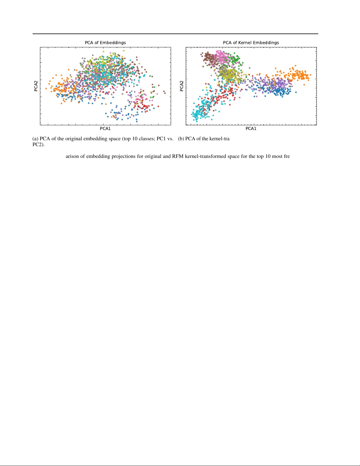
D ANCE: Doubly Adaptiv e Neighborhood Conformal Estimation Brandon R. Feng 1 2 Brian J. Reich 1 Daniel Beaglehole 3 Xihaier Luo 4 David K eetae Park 4 Shinjae Y oo 4 Zhechao Huang 2 Xueyu Mao 2 Olcay Boz 5 Jungeum Kim 1 Abstract The recent de velopments of complex deep learn- ing models hav e led to unprecedented ability to accurately predict across multiple data represen- tation types. Conformal prediction for uncer- tainty quantification of these models has risen in popularity , pro viding adaptiv e, statistically-valid prediction sets. For classification tasks, confor- mal methods ha ve typically focused on utilizing logit scores. For pre-trained models, howe ver , this can result in inef ficient, overly conservati ve set sizes when not calibrated towards the target task. W e propose D ANCE, a doubly locally adap- tiv e nearest-neighbor based conformal algorithm combining two nov el nonconformity scores di- rectly using the data’ s embedded representation. D ANCE first fits a task-adapti ve kernel regres- sion model from the embedding layer before us- ing the learned kernel space to produce the fi- nal prediction sets for uncertainty quantification. W e test against state-of-the-art local, task-adapted and zero-shot conformal baselines, demonstrating D ANCE’ s superior blend of set size ef ficiency and robustness across v arious datasets. 1. Introduction The stunning performance of large, pre-trained, multi-modal models, together with the excitement it has sparked, contin- ues to fuel its quick adoption across man y sectors of society . More specifically , vision-language models (VLMs) ( Rad- ford et al. , 2021 ) ha ve spread in use to diverse areas such as medical tasks ( Bazi et al. , 2023 ; Luo et al. , 2025 ; Moon et al. , 2022 ), remote sensing ( Hu et al. , 2025 ; Zhang et al. , 1 Department of Statistics, North Carolina State Univ er- sity , Raleigh, NC, USA 2 Amazon.com, Seattle, W A, USA 3 Department of Computer Science, Uni versity of California San Diego, San Diego, CA, USA 4 Computational Science Initiative, Brookhav en National Laboratory , Upton, NY , USA 5 Amazon.com, San Diego, W A, USA. Correspondence to: Jungeum Kim < jkim255@ncsu.edu > . 2024 ; Kuckreja et al. , 2024 ), and misinformation detection ( Cekinel et al. , 2025 ; Zhou et al. , 2025 ; T ahmasebi et al. , 2024 ). Y et despite these benefits, relativ ely few people vie w AI systems as fully trustw orthy , in part because the y often function as blac k boxes . This gap between percei ved unre- liability and expected utility creates a persistent tension in widespread adoption. Uncertainty quantification of these black box outputs is a practical way to ease this tension: by explicitly ackno wledging uncertainty in model responses and providing probabilistic assessments of output reliability . T o make black-box VLM predictions usable in practice, we need an uncertainty interface that (i) does not require access to or retraining of the foundation model; and (ii) is statistically meaningful at the user’ s chosen error tol- erance. Conformal prediction (CP) provides a principled, model-agnostic approach for uncertainty quantification in this black-box setting: giv en a user-specified misco verage lev el α , CP wraps any predictor to produce a prediction set that contains the true label with probability at least 1 − α ( V o vk et al. , 2005 ; 1999 ; Lei et al. , 2018 ; Shafer & V o vk , 2008 ). Additionally , many uncertainty quantifi- cation approaches require modeling assumptions about the data-generating distribution ( Gra ves , 2011 ; Gal & Ghahra- mani , 2016 ; Hern ´ andez-Lobato & Adams , 2015 ). In con- trast, conformal prediction is distribution-free, making it easy to deploy across a broad range of problems. The key as- sumption is exchangeability between the calibration dataset and the test dataset, where neither is in volved in the training of the model. The prediction set for each test observ ation is then formed from appropriate calibration set responses based on some nonconformity score. The ease of usage has turned CP into a popular UQ tool for VLMs ( K ostumov et al. , 2024 ; Dutta et al. , 2023 ; Silva-Rodr ´ ıguez et al. , 2025 ). Y et CP’ s distribution-free guarantee often comes with a cost: the resulting prediction sets can be unnecessarily large, especially when the base model’ s confidence scores are mis- aligned with the downstream task ( Lei et al. , 2018 ; Romano et al. , 2019 ; 2020 ; Angelopoulos et al. , 2020 ). For example, consider a simple three-way problem, cat vs. fox vs. dog, handled by an out-of-the-box VLM. If the model assigns similar scores to these semantically related classes, a con- formal method may hedge by returning { cat, fox, dog } to maintain the desired 1 − α cov erage: statistically valid, but 1 Doubly Adaptive Neighborhood Conformal Estimation Figure 1. The D ANCE pipeline. (a) The calibration set is used to compute nonconformity scores for a given test input. Our architectural contribution is the introduction of a task-adapted Recursiv e Feature Machines (RFM) kernel together with two complementary noncon- formity scores. (b) The Neighbor Nonconformity module deriv es a rank cutoff q knn in the kernel space from the calibration set. This cutoff is used to identify nearest labels and to construct the candidate label set ˆ C knn for the test input. (c) The Contrastiv e Nonconformity module defines a density cutof f q clr , below which a second candidate label set ˆ C clr is formed. The intersection of ˆ C knn and ˆ C clr yields the final conformal prediction set ˆ C dance , yielding 1 − α cov erage. operationally uninformative . This has moti vated e xtensive ef forts to improv e efficienc y . In classification, there has been significant focus on set size reduction through areas such as optimal thresholding from LA C ( Sadinle et al. , 2019 ), to nov el nonconformity mea- sures such as APS, RAPS and SAPS ( Romano et al. , 2020 ; Angelopoulos et al. , 2020 ; Huang et al. , 2023 ), and optimal transport weighting ( Silva-Rodr ´ ıguez et al. , 2025 ) to reduce out-of-distribution misalignment for zero-shot prediction. Howe ver , these methods utilize the logit probability layer of the model, losing potential impact from rich embedding information from earlier layers. Local v ariants of CP ha ve of fered a framew ork-based ap- proach to set size reduction. These methods focus on the notion of local exchangeability , where calibration observ a- tions in a local space around the test point are fav ored in prediction set construction, resulting in smaller set sizes due to smaller response v ariation ( Ding et al. , 2023 ; Guan , 2023 ; Mao et al. , 2024 ; Hore & Barber , 2025 ). For e xample, in a spatial regression setting, only calibration observations in a 2-D or 3-D radius around the test are used based on a decay- ing correlation parameter ( Mao et al. , 2024 ; Jiang & Xie , 2024 ; Feng et al. , 2025 ). In classification, approaches such as Deep k -NN ( Papernot & McDaniel , 2018 ) and CONFINE ( Huang et al. , 2024 ) introduce nonconformity scores based directly on the neighborhood label distribution. Both utilize cosine distance for neighbor retriev al. Howe ver , cosine dis- tance is inherently linear , whereas the comple x task-specific relationships may be better described in a non-linear ker - nel space. Meanwhile, approaches such as localized CP ( Guan , 2023 ) and Neighborhood CP ( Ghosh et al. , 2023 ) re- weight existing nonconformity scores. A potential research gap of these methods is they use neighbor information only indir ectly as a scalar weight, rather than explicitly using neighbor distance in the nonconformity metric. W e propose the D ANCE framework, combining two novel locally adaptiv e nonconformity scores based on embedding distance in a fitted kernel-space to pro vide valid prediction sets for classification. D ANCE contributes: • Computationally efficient alignment of the VLM image embedding space to learn a task-adapted kernel space • Introduction of two nonconformity scores dir ectly us- ing neighborhood information. DANCE utilizes one rank-based neighborhood score and one density-based contrastiv e score defined within the learned kernel space. Rather than indirectly incorporating the kernel similarity as weights for e xisting scores, D ANCE directly uses the k ernel neighborhoods to calculate nonconformity . By constructing the nonconformity scores from embeddings adapted in the kernel space, DANCE maximizes the utility of rich repre- sentations provided by pre-trained foundation models. This dual design blends set size efficiency for marginal co ver- age pro vided by the rank-based score with robustness for conditional cov erage provided by the density-based score, yielding compact and reliable prediction sets. 2 Doubly Adaptive Neighborhood Conformal Estimation 2. Preliminaries Problem Statement. Consider an image classification set- ting with images X ∈ X and labels y ∈ Y = { 1 , ..., c } . W e use a fixed, pre-trained image encoder (e.g. CLIP ( Rad- ford et al. , 2021 )), ϕ : X → R d , mapping images to a d -dimensional embedding space. W e are interested in con- structing a prediction set , ˆ C ( . ) ⊆ Y , that ensures marginal cov erage at a user-specified error rate α ∈ (0 , 1) such that for test observation ( X ∗ , y ∗ ) , P ( y ∗ ∈ ˆ C ( ϕ ( X ∗ ))) ≥ 1 − α. 2.1. Split Conformal Prediction Conformal inference ( V o vk et al. , 2005 ; Shafer & V o vk , 2008 ) allows us to construct prediction sets for black-box models with a finite-sample coverage guaran- tee. Consider calibration data (observations) D cal = { ( X 1 , y 1 ) , ..., ( X n , y n ) } , where each X i ∈ X is a feature and y i ∈ Y is a response. For a new , unseen test point ( X n +1 , y n +1 ) , we assume it is exchangeable with D cal , i.e., their joint distrib ution is in variant under permutation. T o apply split conformal prediction, we need a user -specified nonconformity score S measuring the discrepancy between ( X n +1 , y n +1 ) and D cal . Giv en a pre-specified confidence lev el 1 − α , a nonconformity threshold, q , is calculated as the ⌈ (1 − α )(1 + n ) ⌉ th smallest score of { S i } i ∈D cal , where S i = S ( X i , y i ) . Gi ven a test observation X n +1 and cali- bration set D cal , the prediction set for y n +1 is defined as ˆ C ( X n +1 ) = { y ∈ Y | S ( X, y ) ≤ q } . Assuming exchange- ability holds between the test and calibration set, this pre- diction set guarantees P ( y n +1 ∈ ˆ C ( X n +1 )) ≥ 1 − α ( Lei et al. , 2018 ). 2.2. Local Conformal Prediction The frame work of localized conformal prediction w as in- troduced by Guan ( 2023 ), creating more efficient predic- tion set sizes through weighting the nonconformity scores according to some localizer function centered at test obser- vation X n +1 . Broadly , for localizer similarity K n +1 ,i = K ( X n +1 , X i ) ∀ i ∈ 1 , ..., n , calculate probability mass p n +1 ,i = K n +1 ,i / P n +1 j =1 K n +1 ,j to weight scores s i before finding the quantile cutoff in SCP . For calibration neighbors with high dissimilarity , their influence in the nonconformity threshold calibration decreases significantly . Ghosh et al. ( 2023 ) proposed using an exponential k ernel as the localizer such that for some function, ϕ ( . ) of the features, K ( X i , X j ) = exp  −|| ϕ ( X i ) − ϕ ( X j ) || 2 L  , for a tunable bandwidth parameter L . They sho w this k ernel localizer raises the set size efficiency for both regression and classification problems. For classification, intuiti vely , this local weighting ensures the threshold is primarily de- termined by neighbors with similar classes to the given test image, reducing the addition of unrelated classes to the pre- diction set. This idea of localized e xchangeability raising set-size efficienc y serves as a basis for our methodology . 2.3. Recursive Featur e Machines Our method requires learning representati ve nearest neigh- bors for a gi ven task, rather than using pre-trained similar- ities for identification. This is achieved using the Recur- siv e Feature Machine (RFM) model ( Radhakrishnan et al. , 2024 ), an efficient feature-learning method that composes a learned feature importance matrix and a kernel machine, as an adapter for the image embedding space of the VLM. W e define notation for Kernel Ridge Regression (KRR) and RFM below . Define one-hot encoded training responses Y ∈ R n × c where n is the number of training observations and c is the number of classes. Let input embeddings be Z = ϕ ( X ) ∈ R n × d for the training image set, X , and test input embedding be Z n +1 = ϕ ( X n +1 ) ∈ R 1 × d . The RFM is a learned kernel ridge regression defined as f ( Z n +1 ) = K M ( Z n +1 , Z ) β , for a set of coef ficients β ∈ R n × c , obtained through KRR on the learned similarity measure K M from RFM. In this work, we define K M to be a generalized Laplace kernel function K M ( Z 1 , Z 2 ) = exp −  ∥ Z 1 − Z 2 ∥ M L  1 /ξ ! , for bandwidth parameter L , shape factor ξ , and feature importance matrix M ∈ R d × d . Here, ∥ z ∥ M = ( z M z ⊤ ) 1 / 2 indicates the Mahalanobis norm of z . The M matrix learned by RFM is computed as the A verage Gradient Outer Product (A GOP) of a KRR model, capturing the critical features in input space that most influence the prediction function and improving do wnstream prediction performance both prov ably and empirically ( Zhu et al. , 2025 ; Beaglehole et al. , 2025 ; Radhakrishnan et al. , 2025 ). This importance matrix separates RFM from other KRR methods, providing an implicit measure of feature importance. RFM alternates between updates of M and β , thus empha- sizing embedding dimensions based on their utility for the prediction task. W e additionally tune the L, ξ parameters on a validation set to optimize the k ernel used to obtain nearest neighbors in D ANCE. As we see in Figure 2 , k ernel PCA on the RFM kernel embedding space reveals distinct class-wise clustering. Additional details on A GOP computation, KRR and RFM are in Appendix B . 3 Doubly Adaptive Neighborhood Conformal Estimation PCA1 PCA2 PCA of Embeddings Class 21 22 26 27 31 63 75 82 134 186 Class 21 22 26 27 31 63 75 82 134 186 (a) PCA of the original embedding space (top 10 classes; PC1 vs. PC2). PCA1 PCA2 PCA of K er nel Embeddings Class 21 22 26 27 31 63 75 82 134 186 Class 21 22 26 27 31 63 75 82 134 186 (b) PCA of the kernel-transformed embedding space (top 10 classes; PC1 vs. PC2) Figure 2. Comparison of embedding projections for original and RFM kernel-transformed space for the top 10 most frequent classes (represented by colors) of the Imagenet-R dataset. Note the per-class clustering of the transformed kernel space. (a) Original embeddings; (b) Kernel-transformed embeddings. 3. Doubly Adaptive Neighborhood Conf ormal Estimation The proposed conformal algorithm, D ANCE, consists of a mixture of two nov el nonconformity scores, dir ectly uti- lizing neighborhood information within a learned kernel space: a rank-based score (deri ved from neighborhood size) and a density-based score (deriv ed from nearest-neighbor contrastiv e loss). Our design is moti vated by a trade-of f between efficiency and r obustness . • The Rank-Based Scor e ( S knn ) relies on the relati ve ordering of neighbors. It is scale in variant, adapting to variations in embedding density by treating neighbors in sparse and dense regions equally . This adaptivity results in the global threshold producing highly size efficient prediction sets. Ho wever , the performance may depend on the choice of distance metric, e.g., in this context, the kernel fit quality . In sparse re gions, distant noisy neighbors can be treated as relev ant for threshold determination. • The Density-Based Score ( S clr ) relies on contrasti ve similarity of neighbors. It is more r obust , aggregating embedding similarity in a region to identify all plau- sible classes, thus being able to better reach rare ones. Howe ver , this sensitivity to region density can yield larger set sizes, making it more conserv ativ e and less size efficient. On the other hand, the larger set size can increase conditional class-wise robustness. In what follo ws, giv en pre-trained embedding function, ϕ , let the embedded representation of an input image X ∈ X be denoted as Z = ϕ ( X ) and the corresponding labels be de- noted y ∈ Y where Y is the set of all labels. Let the neighbor reference set be defined D ref = { ( ˜ Z j , ˜ y j ) } n ref j =1 and the cali- bration set be defined D cal = { ( Z j , y j ) } n j =1 where D ref is independent from D cal . Define notation N k ( Z, ˜ Z ) ⊆ D ref as the k -nearest neighbors to Z from reference embeddings, ˜ Z , in the learned RFM kernel space, K M ( ., . ) . Nearest neighbors are identified as the k reference set observ ations with minimum pairwise Euclidean distances after embed- dings are projected by the learned feature matrix, M 1 / 2 . 3.1. k -NN Set Nonconformity W e first define a prediction set (hereafter , the k -NN set classifier) that consists of all unique labels appearing among the k nearest neighbors i.e, ˆ L k ( Z ) = Unique { ˜ y ∈ Y | ( ˜ Z , ˜ y ) ∈ N k ( Z, ˜ Z ) } . (1) The philosophy of the k -NN set classifier is based on the same premise of the standard k -NN classifier that the true label for Z is likely to appear among the labels of its k - nearest neighbors. In the following, we conformalize the k - NN set, establishing its finite-set distrib ution-free theoretical cov erage guarantee. For feature-label pairings ( Z, y ) , and neighbor search num- ber m knn ≤ n ref , we define the rank-based nonconformity score as S knn ( Z, y ) = arg min k ∈ [ m knn ] ∪{∞}  y ∈ ˆ L k ( Z )  , (2) where ˆ L ∞ ( Z ) is the set of all labels. Define the conformal threshold q knn by taking the ⌈ (1 − α knn )(1 + n ) ⌉ th smallest 4 Doubly Adaptive Neighborhood Conformal Estimation calibration score on D cal for some error rate α knn . The k - NN conformal prediction set is defined by the set of labels found within neighbor radius q knn , i.e, ˆ C knn ( Z ) = ˆ L q knn ( Z ) , (3) where ˆ L k is defined in ( 1 ) . This conformalized prediction set comes with co verage 1 − α knn as the following theorem. Theorem 3.1. Assume that the calibration sample D cal to- gether with test observation ( Z n +1 , y n +1 ) is exc hangeable. F or the pr ediction set ˆ C knn ( Z n +1 ) defined in ( 3 ) , we have covera ge guarantee 1 − α knn ≤ P  y n +1 ∈ ˆ C knn ( Z n +1 )  ≤ 1 − α knn + 1 n + 1 , wher e the upper bound is established given ther e is no tie among the nonconformity scor es and q knn ≤ m knn . Pr oof. See, Appendix Section C.1 As the S knn score values are discrete, this can result in ties on the calibration set. In this case, the upper bound guarantee does not e xist, which can lead to ov ercover - age, decreasing size ef ficiency . In order to ha ve the upper bound guarantee as well, we add a small amount of noise S knn ( Z, y ) + U ( Z, y ) for U iid ∼ Unif (0 , ϵ ) for some ϵ < 1 . The threshold q knn represents the maximum rank a label may take in a neighborhood to be considered plausible. Intuitiv ely , this imposes a hard constraint on the di versity of labels, where only labels in the top ranks are predicted. For example, an input may only contain “cat” candidate labels within the top ranks, ignoring potentially semantically related animals like “tiger” and “dog” in the embedding space, b ut which fail to reach the cutoff. This prioritizes size efficiency , creating compact sets at the e xpense of potential robustness by e xcluding semantically related classes. 3.2. Ker nel Contrastive Nonconformity Contrasti ve learning seeks to structure the embedding space by minimizing the distance between similar (positive) pairs of samples against a background set of dissimilar (nega- tiv e) ones based only on the input space. The fundamental InfoNCE loss ( Oord et al. , 2018 ; Sohn , 2016 ; W u et al. , 2018 ) was de veloped to achiev e this structure during model training, using augmented v ariants of the same instance to produce positiv e pairs, while pushing away other instances. Dwibedi et al. ( 2021 ) extended this with Nearest Neighbor Contrastiv e Learning Representations (NNCLR). Rather than solely relying on augmentations, they b uild positive pairs using nearest neighbors from a support set, thus utiliz- ing local density information. Our density-based conformity score is based on NNCLR. Let Z i be the embedded representation of our input with label y i and Q ( Z i ) = N m clr ( Z i , ˜ Z ) be the m clr ker - nel nearest neighbors forming the support set. For the nearest-neighbor anchor, A i = N 1 ( Z i , ˜ Z \ Z i ) , and em- bedded neighbor , Z j ∈ Q ( Z i ) , define d K ( A i , Z j ) = 2 · (1 − K M ( A i , Z j )) . For each neighbor Z j ∈ Q ( Z i ) , first calculate pairwise loss: L ( Z i , Z j ) = − log exp( − d K ( A i , Z j ) /τ ) P Z k ∈ Q ( Z i ) exp( − d K ( A i , Z k ) /τ ) . (4) Here, each support set neighbor is treated as the augmen- tation of Z i .The denominator is summed only over the neighborhood Q ( Z i ) rather than the full reference set as in NNCLR. This results in a relati ve measure of local den- sity using our learned kernel space. Then, to conformalize this self-supervised loss, the labels are used to determine the required similarity between inputs for the desired outcome. The NNCLR-based nonconformity score is defined as the minimum loss among neighbors sharing the same label as y i . This is formalized as S clr ( Z i , y i ) = min {L ( Z i , Z j ) | Z j ∈ Q ( Z i ) , y j = y i } . (5) Define the conformal threshold q clr by taking the ⌈ (1 − α clr )(1 + n ) ⌉ th smallest calibration score on D cal for some error rate α clr . Thus the CLR conformal prediction set with cov erage 1 − α clr is ˆ C clr ( Z ) = { y ∈ Y | S clr ( Z, y ) ≤ q clr } . (6) Follo wing directly from Theorems 2.1 and 2.2 in Lei et al. ( 2018 ), the coverage, P  y n +1 ∈ ˆ C clr ( Z n +1 )  , can be bounded below by 1 − α clr and abo ve by 1 − α clr + 1 n +1 . The threshold q clr represents the minimum relative simi- larity a candidate must share with an input compared to other local points. Intuitively , this captures representation grouping structure in the kernel space where semantically similar classes (i.e. cat, dog, tiger) may be predicted to- gether , regardless of class imbalance. Thus, this score raises r obustness at the e xpense of size. 3.3. D ANCE W e define the Doubly Adapti ve Neighborhood Conformal Estimation (D ANCE) prediction set as: ˆ C dance ( Z ) = ˆ C knn ( Z ) ∩ ˆ C clr ( Z ) . (7) The combination is moti vated by the complementary geo- metric properties of the two scores. Intuiti vely , by inter- secting the irregular , discrete boundaries of the k -NN rank score with the smoother , continuous boundaries of the CLR density score, D ANCE retains the semantic groupings cap- tured by the latter while applying the former as a cardinality 5 Doubly Adaptive Neighborhood Conformal Estimation constraint to prune extraneous classes. Thus, controlling q knn is critical as it explicitly caps the maximum size of the D ANCE prediction set. Assume the total error rate is set as α = α knn + α clr . W e introduce h yperparameter λ to control the division such that α clr = λ · α and α knn = (1 − λ ) · α . This leads to the following proposition for coverage guaran- tee. Proposition 3.2. Under the assumptions of Theorem 3.1 , let ˆ C knn ( Z n +1 ) be the prediction set defined in ( 3 ) . Addi- tionally , let ˆ C clr ( Z n +1 ) be constructed under valid split conformal prediction conditions. F or intersection set ˆ C dance ( Z n +1 ) = ˆ C knn ( Z n +1 ) ∩ ˆ C clr ( Z n +1 ) , we have: P ( y n +1 ∈ ˆ C dance ( Z n +1 )) ≥ 1 − α knn − α clr . Pr oof. See, Section C.2 Finally , Algorithm 1 found in Appendix A depicts the con- struction of ˆ C dance ( Z ) . 4. Experiments 4.1. Setup 4 . 1 . 1 . D A TA D E S C R I P T I O N D ANCE’ s performance is ev aluated across 11 common im- age classification datasets. For more gener alized datasets spanning a wide variety of subjects, we test the ImageNet variants of ImageNet ( Deng et al. , 2009 ), ImageNet-R ( Hendrycks et al. , 2021 ), and ImageNet-Sk etch ( W ang et al. , 2019 ). For more focused datasets on a single topic, we use EuroSA T ( Helber et al. , 2019 ), StanfordCars ( Krause et al. , 2013 ), Food101 ( Bossard et al. , 2014 ), OxfordPets ( Parkhi et al. , 2012 ), Flowers102 ( Nilsback & Zisserman , 2008 ), Caltech101 ( Fei-Fei et al. , 2004 ), DTD ( Cimpoi et al. , 2014 ) and UCF101 ( Soomro et al. , 2012 ). W e only use the av ailable test set of each dataset for this study . Each dataset is randomly split into 40% for RFM kernel fitting ( D sup ), 40% for the calibration set ( D cal ) and 20% for the testing set ( D T est ). For fitting the RFM model and kernel hyperparameters, the training set is split into 80% for training and 20% v alidation. For test conformal prediction results, each observation in the test set draws neighbors from the entire calibration set. Our methodology coverage guarantees apply to fully dis- joint reference/calibration splits. Howe ver , to improve data efficienc y in finite-sample experiments, we also ev aluate a calibration-reuse setting where D cal is reused as reference set D ref . Specifically , when computing calibration noncon- formity scores, for each Z i ∈ D cal , neighbors are found based via a leav e-one-out search where D ref = D cal \{ Z i } to a void self-matching. Similar reuse strategies ha ve pre- viously been used in neighbor -based methods ( Papernot & McDaniel , 2018 ; Ghosh et al. , 2023 ). Thus, we report em- pirical results under this reuse setting. Additionally , we empirically corroborate this choice against a theoretically- valid disjoint split in Appendix D , demonstrating closely matching cov erage and UQ performance. For f airness, all local CP methods compared reuse the D cal as D ref . 4 . 1 . 2 . I M P L E M E N T AT I O N D E TA I L S W e use pre-trained CLIP models with two different back- bones: ResNet-101, representing a CNN-based backbone, and V iT -B/16, representing a transformer -based backbone. For D ANCE, the pre-trained image encoder is used to em- bed the images into the features used for k ernel fitting and the conformal procedure. The RFM model serves as a task adapter and hyperparameter optimization of the kernel is done through a Bayesian optimization approach for 25 total ev aluations, with accuracy as the objecti ve. T o determine the optimal ratio for λ , D cal is first split into 80% calibration and 20% validation. This is then used in a grid search ov er λ ∈ [0 , 1] with a step size of 0.1. After selection, λ is fixed and the final conformal thresholds are computed on the full D cal . For all datasets, the neighbor- hood sizes are set at m knn = 100 and m clr = 50 and tem- perature τ = 0 . 01 . W e provide results for α ∈ [0 . 1 , 0 . 05] . The impact of neighbor choice can be seen in Appendix E . Details on λ selection are gi ven in Appendix F . In addi- tion to DANCE, we also ev aluate k -NN Set and CLR Set, representing D ANCE with λ fixed at 0 and 1 , respectively . W e compare to the commonly-used nonconformity scores of APS ( Romano et al. , 2020 ) and RAPS ( Angelopoulos et al. , 2020 ) based on perturbed logit rankings. T o strictly isolate the contribution of the nonconformity scores of DANCE from the feature learning benefits of the RFM k ernel, we utilize the same RFM-adapted backbone in two baseline framew orks. The first, RFM Adapter , represents a non- localized baseline where APS and RAPS are applied directly on the logits predicted by the RFM adapter . The second, Neighborhood Conf ormal Prediction (NCP) ( Ghosh et al. , 2023 ), represents a similar localized approach where the RFM-predicted logits are re-weighted based on Euclidean distance in a tuned kernel space before being used in RAPS calculations. For NCP , we look at the nearest 50 neighbors as it is most similar to the clr scoring format. Next, we also compare APS and RAPS used in Conf-O T ( Silva-Rodr ´ ıguez et al. , 2025 ), a state-of-the-art zero-shot approach using optimal transport to align the logit space with the calibration class distribution. F or Conf-O T , we follow the original setup where CLIP logits are deriv ed from image/text pairs using standard text templates ( Gao et al. , 2024 ; Zhou et al. , 2022 ). W e note that Conf-O T is the only method tested that uses the CLIP te xt encoder to construct class prototypes, where the other methods use only 6 Doubly Adaptive Neighborhood Conformal Estimation α = 0 . 1 α = 0 . 05 Method Acc Size Cov Cov Range CCV Size Cov Cov Range CCV D ANCE (Ours) 0.856 2.49 0.930 (0.903, 0.964) 8.442 4.96 0.963 (0.949, 0.986) 5.364 k -NN Set (Ours) 0.856 2.33 0.921 (0.902, 0.956) 8.877 4.77 0.958 (0.949, 0.971) 5.785 CLR Set (Ours) 0.856 5.82 0.936 (0.913, 0.974) 8.128 8.20 0.965 (0.955, 0.989) 5.346 Deep k -NN 0.856 4.26 0.936 (0.905, 0.987) 8.799 7.50 0.967 (0.951, 0.998) 5.265 RFM Adapter (APS) 0.856 2.23 0.904 (0.897, 0.917) 8.817 5.28 0.952 (0.945, 0.957) 5.948 RFM Adapter (RAPS) 0.856 2.21 0.904 (0.895, 0.919) 8.854 5.29 0.952 (0.943, 0.957) 5.979 NCP (RAPS) 0.856 2.48 0.935 (0.895, 0.974) 8.846 5.81 0.958 (0.936, 0.983) 5.721 Conf-O T (APS) 0.720 6.04 0.902 (0.889, 0.925) 8.436 9.98 0.953 (0.944, 0.964) 5.846 Conf-O T (RAPS) 0.720 5.29 0.903 (0.890, 0.925) 8.503 8.10 0.953 (0.948, 0.962) 5.803 T able 1. CLIP V iT -B/16: A verage accuracy and UQ quality metrics (Set Size, Co verage, Coverage Range, Class-conditional Cov erage V iolation) across 11 datasets. Best and second best set size and CCV are bolded and underlined, respectiv ely . α = 0 . 1 α = 0 . 05 Method Acc Size Cov Cov Range CCV Size Cov Cov Range CCV D ANCE (Ours) 0.820 4.11 0.926 (0.900, 0.957) 8.746 8.07 0.962 (0.946, 0.976) 5.627 k -NN Set (Ours) 0.820 4.03 0.920 (0.900, 0.961) 9.006 8.47 0.957 (0.950, 0.973) 5.963 CLR Set (Ours) 0.820 7.49 0.903 (0.903, 0.970) 8.626 9.96 0.965 (0.945, 0.989) 5.430 Deep k -NN 0.820 5.66 0.935 (0.904, 0.989) 8.855 11.58 0.972 (0.957, 1.000) 5.018 RFM Adapter (APS) 0.820 3.13 0.904 (0.890, 0.915) 8.761 8.96 0.954 (0.946, 0.963) 5.982 RFM Adapter (RAPS) 0.820 3.12 0.903 (0.890, 0.913) 8.796 8.98 0.954 (0.946, 0.963) 6.002 NCP (RAPS) 0.820 3.38 0.926 (0.888, 0.958) 8.904 8.85 0.960 (0.937, 0.984) 5.660 Conf-O T (APS) 0.661 8.44 0.907 (0.893, 0.928) 8.604 13.95 0.954 (0.948, 0.973) 5.820 Conf-O T (RAPS) 0.661 7.39 0.907 (0.897, 0.926) 8.651 11.57 0.955 (0.950, 0.981) 5.859 T able 2. CLIP ResNet-101: A verage accuracy and UQ quality metrics (Set Size, Coverage, Co verage Range, Class-conditional Coverage V iolation) across 11 datasets. Best and second best set size and CCV are bolded and underlined, respectiv ely . the image encoder . Howe ver , due to its zero-shot nature, prediction accurac y is lo wer as a result. For the RAPS score, hyperparameters λ RAP S and k RAP S are respectiv ely set to 0.001 and 1 for the RFM Adapter and Conf-O T methods. In NCP , these are tuned in a grid search. Finally , we also compare against a 1-layer v ariant of Deep k -NN ( Papernot & McDaniel , 2018 ), representing another method constructing the nonconformity score directly from neighbor information. Their nonconformity score is the pro- portion of neighbors with the correct label, gi ven a neigh- borhood size. W e again utilize the RFM-adapter and obser- vations are e xtracted from the layer corresponding to the RFM kernel-transformed embedding space. W e look at the 75 kernel nearest neighbors, as used in the original paper . All experimental trials were conducted on a workstation equipped with an Intel Core i9-14900KF processor , 64 GB of 5200 MHz RAM, and an NVIDIA GeForce R TX 4090 GPU with 24 GB of VRAM. W e utilize the open-source implementations pro vided by the authors for NCP and Conf- O T . 4 . 1 . 3 . P E R F O R M A N C E M E T R I C S The performance of all the methods are e valuated on both classification and UQ quality on the held test set. The T op-1 accuracy (Acc) is used for classification quality . Overall cov erage (Co v) and set size (Size) are used as to measure marginal UQ quality , and class-conditional cov erage viola- tion (CCV) ( Ding et al. , 2023 ) is used to measure conditional UQ quality . CCV is defined as C C V = 100 × 1 |Y | X y ∈Y | ˆ Cov y − (1 − α ) | , where |Y | is the total number of classes, and ˆ Cov y is the cov erage for class y ∈ Y . While overall coverage places more weight on highly represented classes, CCV balances the influence of large and small classes, thus being a metric reflecting r obustness to class distribution. W e report average accuracy , coverage, set-size and coverage gap, as well as cov erage range across all datasets. The results for indi vidual datasets in the α = 0 . 05 setting for CLIP V iT -B/16 are giv en in Appendix G.2 . Finally , we note that D ANCE is computationally efficient: 7 Doubly Adaptive Neighborhood Conformal Estimation                   λ                            (a) A verage Cov erage (Min/Max)                   λ             (b) A verage Set Size                   λ                    (c) A verage CCV Figure 3. Ablation study of UQ based on λ . W e observe the mix of S knn and S clr generally provides a trade-of f between CCV and set size. the full λ grid search required an av erage of 4.0 seconds (range: 0 . 2 s – 19 . 1 s ), with mean total inference time taking an av erage of 0 . 08 s (range: < 1 ms– 0 . 33 s). 4.2. Main Results T able 1 shows results using embeddings from the CLIP V iT -B/16 backbone. At the relaxed error rate of α = 0 . 1 , RFM Adapter (RAPS) achie ves the lowest a verage set size (2.21), with the APS variant follo wing closely (2.23). CLR Set sho ws its rob ustness properties, with the lowest CCV (8.128), albeit with high set size (5.82), predicting over twice as man y classes on a verage compared to more efficient baselines. DANCE achiev es third best CCV (8.442), with comparable set size efficienc y (2.49) to the top competitors. The benefits of D ANCE are more pronounced for the more conservati ve α = 0 . 05 . The combination of properties is exhibited here where it achiev es nearly the same conditional performance in robustness as CLR Set (5.364 vs 5.346), with the set size efficiency brought by the most efficient k -NN Set (4.96 vs 4.77). These account for the second and third best in CCV and the top two in set size. This has lower set size than the closest baseline of RFM Adapter with APS (5.28) and slightly higher CCV than the top Deep k -NN (5.265), highlighting D ANCE’ s ability to optimize both ef ficiency and robustness without excelling in only one. T able 2 shows results using embeddings from the CLIP ResNet-101 backbone. The lower a verage accuracy (0.820 vs 0.856) makes uncertainty quantification more challeng- ing, albeit with similar results. At α = 0 . 05 , DANCE shines, providing the lo west av erage set size (8.07) with third low- est CCV (5.627), further validating its capacity for high efficienc y and conditional robustness. For both backbones, we note the high robustness of the Conf-O T and relative size efficienc y , despite the lo wer zero-shot prediction accuracy , indicating benefits of using the te xt embeddings from the multi-modal model. Coverage range re veals undercov erage for some baselines, where individual dataset performance drops to 0.89 for α = 0 . 1 and belo w 0.94 for α = 0 . 05 . In contrast, D ANCE attains near-nominal empirical co verage across all experiments under this reuse setting. 4 . 2 . 1 . λ S E N S I T I V I T Y Figure 3 shows the effect of λ on the UQ metrics of coverage, set size and CCV for CLIP V iT -B/16 at α = 0 . 05 based on λ ∈ [0 , 0 . 1 , 0 . 25 , 0 . 5 , 0 . 75 , 0 . 9 , 1] . W e see the optimal cov erage and CCV generally lies between the k nn and clr scores on their own, with spikes in a verage CCV at both ends and an increasing av erage set size as λ fa vors clr . This indicates the need for the grid search step to find the balance. D ANCE also maintains marginal cov erage for all λ values. 5. Conclusion In this w ork, we introduce D ANCE (Doubly Adaptive Neighborhood Conformal Estimation), a nov el framework that provides v alid uncertainty quantification for pre-trained vision-language models. By operating within an efficiently learned kernel space rather than fixed pre-trained embed- dings, D ANCE effecti vely captures complex non-linear re- lationships between calibration and test set that is le veraged in set construction while also maximizing utility of the de- scriptiv eness these embeddings provide. Our ke y methodological contribution lies in the synergistic blend of two novel neighbor-based nonconformity scores: a rank-based score, S knn , that ensures efficiency through a hard size cutoff, and a density-based score, S clr , that promotes robustness through returning semantically-related groups. Through extensi ve e xperiments on CLIP adaptation, we demonstrate that this dual-score approach, optimized via a learned mixing parameter λ , consistently achie ves a high balance of tight prediction sets and high conditional cov erage validity compared to state-of-the-art baselines. W e note there are limitations of D ANCE. First, the effi- ciency and rob ustness hinges on the fit of the kernel. If the 8 Doubly Adaptive Neighborhood Conformal Estimation RFM kernel is a poor fit, the local embedding clustering can be dif fuse, causing inefficient set sizes with high cutof f for q knn and the inclusion of ov erly robust neighborhoods from q clr . The final set efficienc y and robustness also depends on choice of λ , m knn and m clr , making tuning an essential part. Second, in limited data settings, the reference and calibra- tion sets may need to be reused, losing the strict theoretical cov erage guarantees provided. Nevertheless, we see that D ANCE maintains empirical coverage v alidity across all experiments and an ablation showed no significant de viation between this heuristic split and a valid disjoint split. Future work can extend this method to both continuous and genera- tiv e settings, with small outcome-dependent changes to the nonconformity scores. The performance of the contrastiv e score may also benefit in a true multi-modal setting, where more embeddings sources are used to calculate semantic similarity . The robust performance of the zero-shot Conf- O T baseline against task-adapted competitors previe ws the predictiv e power multi-modal representations can bring. Acknowledgements W e thank Mikhail Belkin, Qi Zhao and Zhanlong Qiu for in valuable discussions on RFM, contrastive learning and kernel nearest neighbors. References Angelopoulos, A., Bates, S., Malik, J., and Jordan, M. I. Uncertainty sets for image classifiers using conformal prediction. arXiv pr eprint arXiv:2009.14193 , 2020. Bazi, Y ., Rahhal, M. M. A., Bashmal, L., and Zuair, M. V ision–language model for visual question answering in medical imagery . Bioengineering , 10(3):380, 2023. Beaglehole, D., Holzm ¨ uller , D., Radhakrishnan, A., and Belkin, M. xrfm: Accurate, scalable, and interpretable feature learning models for tab ular data. arXiv pr eprint arXiv:2508.10053 , 2025. Bossard, L., Guillaumin, M., and V an Gool, L. Food-101– mining discriminati ve components with random forests. In Eur opean confer ence on computer vision , pp. 446–461. Springer , 2014. Cekinel, R. F ., Karagoz, P ., and C ¸ ¨ oltekin, C ¸ . Multimodal fact-checking with vision language models: A probing classifier based solution with embedding strategies. In Pr oceedings of the 31st International Confer ence on Com- putational Linguistics , pp. 4622–4633, 2025. Cimpoi, M., Maji, S., Kokkinos, I., Mohamed, S., and V edaldi, A. Describing textures in the wild. In Pr o- ceedings of the IEEE confer ence on computer vision and pattern r ecognition , pp. 3606–3613, 2014. Deng, J., Dong, W ., Socher , R., Li, L.-J., Li, K., and Fei-Fei, L. Imagenet: A lar ge-scale hierarchical image database. In 2009 IEEE conference on computer vision and pattern r ecognition , pp. 248–255. Ieee, 2009. Ding, T ., Angelopoulos, A., Bates, S., Jordan, M., and T ib- shirani, R. J. Class-conditional conformal prediction with many classes. Advances in neural information pr ocessing systems , 36:64555–64576, 2023. Dutta, S., W ei, H., van der Laan, L., and Alaa, A. M. Esti- mating uncertainty in multimodal foundation models us- ing public internet data. arXiv pr eprint arXiv:2310.09926 , 2023. Dwibedi, D., A ytar, Y ., T ompson, J., Sermanet, P ., and Zisserman, A. W ith a little help from my friends: Nearest- neighbor contrastiv e learning of visual representations. In Pr oceedings of the IEEE/CVF international confer ence on computer vision , pp. 9588–9597, 2021. Fei-Fei, L., Fergus, R., and Perona, P . Learning generati ve visual models from few training examples: An incremen- tal bayesian approach tested on 101 object categories. In 2004 confer ence on computer vision and pattern r ecogni- tion workshop , pp. 178–178. IEEE, 2004. Feng, B. R., Park, D. K., Luo, X., Urdangarin, A., Y oo, S., and Reich, B. J. Staci: Spatio-temporal aleatoric conformal inference. arXiv preprint , 2025. Gal, Y . and Ghahramani, Z. Dropout as a bayesian approx- imation: Representing model uncertainty in deep learn- ing. In international conference on machine learning , pp. 1050–1059. PMLR, 2016. Gao, P ., Geng, S., Zhang, R., Ma, T ., F ang, R., Zhang, Y ., Li, H., and Qiao, Y . Clip-adapter: Better vision-language models with feature adapters. International Journal of Computer V ision , 132(2):581–595, 2024. Ghosh, S., Belkhouja, T ., Y an, Y ., and Doppa, J. R. Im- proving uncertainty quantification of deep classifiers via neighborhood conformal prediction: Novel algorithm and theoretical analysis. In Proceedings of the AAAI Confer- ence on Artificial Intelligence , volume 37, pp. 7722–7730, 2023. Grav es, A. Practical variational inference for neural net- works. Advances in neural information pr ocessing sys- tems , 24, 2011. Guan, L. Localized conformal prediction: A generalized in- ference framew ork for conformal prediction. Biometrika , 110(1):33–50, 2023. 9 Doubly Adaptive Neighborhood Conformal Estimation Helber , P ., Bischke, B., Dengel, A., and Borth, D. Eurosat: A novel dataset and deep learning benchmark for land use and land cov er classification. IEEE Journal of Se- lected T opics in Applied Earth Observations and Remote Sensing , 12(7):2217–2226, 2019. Hendrycks, D., Basart, S., Mu, N., Kada vath, S., W ang, F ., Dorundo, E., Desai, R., Zhu, T ., Parajuli, S., Guo, M., et al. The man y faces of rob ustness: A critical analysis of out-of-distribution generalization. In Pr oceedings of the IEEE/CVF international confer ence on computer vision , pp. 8340–8349, 2021. Hern ´ andez-Lobato, J. M. and Adams, R. Probabilistic back- propagation for scalable learning of bayesian neural net- works. In International confer ence on mac hine learning , pp. 1861–1869. PMLR, 2015. Hore, R. and Barber , R. F . Conformal prediction with local weights: randomization enables robust guarantees. Jour- nal of the Royal Statistical Society Series B: Statistical Methodology , 87(2):549–578, 2025. Hu, Y ., Y uan, J., W en, C., Lu, X., Liu, Y ., and Li, X. Rsgpt: A remote sensing vision language model and benchmark. ISPRS J ournal of Photogrammetry and Remote Sensing , 224:272–286, 2025. Huang, J., Xi, H., Zhang, L., Y ao, H., Qiu, Y ., and W ei, H. Conformal prediction for deep classifier via label ranking. arXiv pr eprint arXiv:2310.06430 , 2023. Huang, L., Lala, S., and Jha, N. K. Confine: Conformal pre- diction for interpretable neural networks. arXiv pr eprint arXiv:2406.00539 , 2024. Jiang, H. and Xie, Y . Spatial conformal inference through localized quantile regression. arXiv pr eprint arXiv:2412.01098 , 2024. K ostumov , V ., Nutfullin, B., Pilipenko, O., and Ilyushin, E. Uncertainty-aw are e valuation for vision-language models. arXiv pr eprint arXiv:2402.14418 , 2024. Krause, J., Stark, M., Deng, J., and Fei-Fei, L. 3d object rep- resentations for fine-grained categorization. In Pr oceed- ings of the IEEE international confer ence on computer vision workshops , pp. 554–561, 2013. Kuckreja, K., Danish, M. S., Naseer , M., Das, A., Khan, S., and Khan, F . S. Geochat: Grounded large vision- language model for remote sensing. In Pr oceedings of the IEEE/CVF Confer ence on Computer V ision and P attern Recognition , pp. 27831–27840, 2024. Lei, J., G’Sell, M., Rinaldo, A., T ibshirani, R. J., and W asserman, L. Distribution-free predicti ve inference for regression. Journal of the American Statistical Associa- tion , 113(523):1094–1111, 2018. Luo, L., T ang, B., Chen, X., Han, R., and Chen, T . V ividmed: V ision language model with versatile visual grounding for medicine. In Pr oceedings of the 2025 Conference of the Nations of the Americas Chapter of the Associa- tion for Computational Linguistics: Human Language T echnologies (V olume 1: Long P apers) , pp. 1800–1821, 2025. Mao, H., Martin, R., and Reich, B. J. V alid model-free spatial prediction. J ournal of the American Statistical Association , 119(546):904–914, 2024. Moon, J. H., Lee, H., Shin, W ., Kim, Y .-H., and Choi, E. Multi-modal understanding and generation for medical images and text via vision-language pre-training. IEEE Journal of Biomedical and Health Informatics , 26(12): 6070–6080, 2022. Nilsback, M.-E. and Zisserman, A. Automated flower clas- sification over a large number of classes. In 2008 Sixth Indian confer ence on computer vision, gr aphics & ima ge pr ocessing , pp. 722–729. IEEE, 2008. Nogueira, F . Bayesian Optimization: Open source constrained global optimization tool for Python, 2014–. URL https:// github.com/bayesian- optimization/ BayesianOptimization . Oord, A. v . d., Li, Y ., and V inyals, O. Representation learn- ing with contrastive predictiv e coding. arXiv preprint arXiv:1807.03748 , 2018. Papernot, N. and McDaniel, P . Deep k-nearest neighbors: T ow ards confident, interpretable and rob ust deep learning. arXiv pr eprint arXiv:1803.04765 , 2018. Parkhi, O. M., V edaldi, A., Zisserman, A., and Jawahar , C. Cats and dogs. In 2012 IEEE confer ence on computer vision and pattern reco gnition , pp. 3498–3505. IEEE, 2012. Radford, A., Kim, J. W ., Hallacy , C., Ramesh, A., Goh, G., Agarwal, S., Sastry , G., Askell, A., Mishkin, P ., Clark, J., et al. Learning transferable visual models from natural language supervision. In International confer ence on machine learning , pp. 8748–8763. PmLR, 2021. Radhakrishnan, A., Beaglehole, D., P andit, P ., and Belkin, M. Mechanism for feature learning in neural networks and backpropagation-free machine learning models. Sci- ence , 383(6690):1461–1467, 2024. Radhakrishnan, A., Belkin, M., and Drusvyatskiy , D. Linear recursi ve feature machines pro vably recover low-rank ma- trices. Pr oceedings of the National Academy of Sciences , 122(13):e2411325122, 2025. 10 Doubly Adaptive Neighborhood Conformal Estimation Romano, Y ., Patterson, E., and Candes, E. Conformalized quantile regression. Advances in neural information pr o- cessing systems , 32, 2019. Romano, Y ., Sesia, M., and Candes, E. Classification with v alid and adaptive co verage. Advances in neural informa- tion pr ocessing systems , 33:3581–3591, 2020. Sadinle, M., Lei, J., and W asserman, L. Least ambiguous set-valued classifiers with bounded error le vels. Journal of the American Statistical Association , 114(525):223– 234, 2019. Shafer , G. and V ovk, V . A tutorial on conformal prediction. Journal of Mac hine Learning Resear ch , 9(3), 2008. Silva-Rodr ´ ıguez, J., Ben A yed, I., and Dolz, J. Conformal prediction for zero-shot models. In Pr oceedings of the Computer V ision and P attern Recognition Conference , pp. 19931–19941, 2025. Sohn, K. Improved deep metric learning with multi-class n-pair loss objectiv e. Advances in neural information pr ocessing systems , 29, 2016. Soomro, K., Zamir , A. R., and Shah, M. Ucf101: A dataset of 101 human actions classes from videos in the wild. arXiv pr eprint arXiv:1212.0402 , 2012. T ahmasebi, S., M ¨ uller-Budack, E., and Ewerth, R. Mul- timodal misinformation detection using large vision- language models. In Pr oceedings of the 33r d A CM In- ternational Confer ence on Information and Knowledge Management , pp. 2189–2199, 2024. V ovk, V ., Gammerman, A., and Saunders, C. Machine- learning applications of algorithmic randomness. 1999. V ovk, V ., Gammerman, A., and Shafer, G. Algorithmic learning in a random world , v olume 29. Springer, 2005. W ang, H., Ge, S., Lipton, Z., and Xing, E. P . Learning robust global representations by penalizing local predic- tiv e power . Advances in neural information processing systems , 32, 2019. W u, Z., Xiong, Y ., Y u, S. X., and Lin, D. Unsupervised feature learning via non-parametric instance discrimina- tion. In Pr oceedings of the IEEE confer ence on computer vision and pattern r ecognition , pp. 3733–3742, 2018. Zhang, W ., Cai, M., Zhang, T ., Zhuang, Y ., and Mao, X. Earthgpt: A univ ersal multimodal large language model for multisensor image comprehension in remote sensing domain. IEEE T ransactions on Geoscience and Remote Sensing , 62:1–20, 2024. Zhou, K., Y ang, J., Loy , C. C., and Liu, Z. Learning to prompt for vision-language models. International Jour - nal of Computer V ision , 130(9):2337–2348, 2022. Zhou, M., Zhang, L., Horng, S., Chen, M., Huang, K.-H., and Chang, S.-F . M2-tabfact: Multi-document multi- modal fact verification with visual and textual representa- tions of tabular data. In Findings of the Association for Computational Linguistics: ACL 2025 , pp. 26239–26256, 2025. Zhu, L., Da vis, D., Drusvyatskiy , D., and Fazel, M. Itera- ti vely reweighted k ernel machines efficiently learn sparse functions. arXiv pr eprint arXiv:2505.08277 , 2025. 11 Doubly Adaptive Neighborhood Conformal Estimation A. D ANCE Algorithm Algorithm 1 D ANCE Conformal Label Sets 1: Input: Reference embeddings Z ref , Calibration embeddings Z C al , calibration labels y C al , test embedding Z n +1 , learned Kernel K M ( . ) , total error α , error allocation parameter λ 2: Output: Prediction sets { b C i } n test i =1 3: Calibration: compute scores and threshold 4: for i = 1 to n cal do 5: Find all neighbor indices I C al from K M ( Z C al , Z ref ) 6: Compute S knn from Z C al,i to its m knn neighbors index ed by I C al,k nn [ i, :] 7: Compute S clr from Z C al,i to its m clr neighbors index ed by I C al,clr [ i, :] 8: end for 9: Calculate α knn , α clr based on λ split of α 10: Find q knn , q clr from 1 − ( α knn , α clr ) quantiles 11: T est: build label set 12: Find all neighbor indices I n +1 from K M ( Z n +1 , Z ref ) 13: Compute S knn from Z n +1 to its m knn neighbors index ed by I n +1 ,knn 14: Build ˆ C knn ( Z n +1 ) = ˆ Y q knn ( Z n +1 ) 15: Compute S clr from Z n +1 to its m clr neighbors index ed by I n +1 ,clr 16: Build ˆ C clr ( Z n +1 ) from neighbor labels 17: Return: ˆ C dance ( Z n +1 ) = ˆ C knn ∩ ˆ C clr B. T echnical details of Recursive F eature Machines (RFMs) RFMs are an iterative algorithm for learning features with general machine learning models by learning representations through the A verage Gradient Outer Product (A GOP) ( Radhakrishnan et al. , 2024 ). RFMs are initialized with a base prediction algorithm, training inputs and labels, and validation inputs and labels. RFMs fit the training data through T iterations of the following steps. RFM (1) first fits the base algorithm to the training data, (2) computes the A GOP of the fit algorithm from step 1, (3) transforms the data with the A GOP matrix, then (4) returns to step 1. The iteration proceeds for T steps, each step constructing a separate predictor . The best predictor among the iterations is selected on the v alidation set. In our case, as is typically done, we perform the RFM update with K ernel Ridge Regression (KRR) as the base model. W e briefly explain the KRR model. KRR Let X ∈ R n × d denote training samples with x ( i ) T denoting the sample in the i th ro w of X for i ∈ [ n ] and y ∈ R n × c denote training labels, where c is the number of output channels (e.g. one-hot encoded classes for c > 2 classes). In our case, the inputs are themselves embeddings obtained from the internal activ ations of parent models such as CLIP or ResNet. Let K : R d × R d → R denote a kernel function (a positiv e semi-definite, symmetric function), such as the generalized Laplacian kernel we deploy in D ANCE. Giv en a ridge re gularization parameter λ ≥ 0 , KRR solved on the data ( X, y ) giv es a predictor , ˆ f : R d → R c , of the form: ˆ f ( x ) = K ( x, X ) β , (8) where β is the solution to the following linear system: ( K ( X, X ) + λI ) β = y . (9) Here the notation K ( x, X ) ∈ R 1 × n is the n -dimensional ro w vector with K ( x, X ) i = K ( x, x ( i ) ) and K ( X, X ) ∈ R n × n denotes the kernel matrix of pair-wise kernel e valuations K ( X, X ) ij = K ( x ( i ) , x ( j ) ) . The advantage of kernel functions in the context of this w ork is that the predictor admits a closed form solution, which can be robustly computed and generally has fast training times for datasets under 70 k samples. 12 Doubly Adaptive Neighborhood Conformal Estimation A GOP The M matrix learned by RFM is computed as the A verage Gradient Outer Product (A GOP) of a KRR model. For a giv en trained predictor g : R d → R c and its training inputs x 1 , . . . , x n ∈ R d , the A GOP operator produces a matrix A GOP( g , { x i } n i =1 ) = 1 n n X i =1 ∇ g ( x i ) ∇ g ( x i ) ⊤ ∈ R d × d , where ∇ g ∈ R d × c is the (transposed) input-output Jacobian of the function g . The AGOP matrix of a predictor captures the critical features in input space that most influence the prediction function, provably and empirically impro ving downstream prediction performance when used as a feature extractor ( Zhu et al. , 2025 ; Beaglehole et al. , 2025 ; Radhakrishnan et al. , 2025 ). RFMs W e outline the particular RFM algorithm used in our work belo w . Given that the procedure is the same for an y block, we simplify notation by omitting the block subscripts ℓ . For any x, z ∈ R k , choice of bandwidth parameter L > 0 , and a positiv e semi-definite, symmetric matrix M ∈ R k × k and K M Mahalanobis kernel function, let K M ( Z, z ) ∈ R n such that K M ( Z, z ) i = K M ( a ( i ) , z ) and let K M ( Z, Z ) ∈ R n × n such that K M ( Z, Z ) i,j = K M ( a ( i ) , a ( j ) ) . Letting M 0 = I and λ ≥ 0 denote a regularization parameter , RFM repeats the following tw o steps for T iterations: Step 1: ˆ f t ( z ) = β t K M t ( Z, z ) where β t = y [ K M t ( Z, Z ) + λI ] − 1 , (Kernel ridge re gression) Step 2: M t +1 = 1 n n X i =1 ∇ z ˆ f t ( a ( i ) ) ∇ z ˆ f t ( a ( i ) ) ⊤ ; (A GOP) where ∇ z ˆ f t ( a ( i ) ) denotes the gradient of ˆ f t with respect to the input z at the point a ( i ) . W e utilize the xRFM repo for the RFM implementation ( Beaglehole et al. , 2025 ) C. Proof of Theor ems C.1. Proof of Theorem 3.1 Pr oof. Recall the definition of set-valued k NN classifier: ˆ L k ( Z ) = Unique { ˜ y ∈ Y | ˜ y ∈ N k ( Z, ˜ Z ) } , where the neighborhood is searched ov er a reference dataset, D ref , that is independent of {D cal , ( Z n +1 , y n +1 ) } . Here, we add a bit of a technical tool. Assume the classifier model returns the set of prediction sets, f ( x ) = { ˆ L 1 ( Z ) , ..., ˆ L m knn ( Z ) } ∪ { ˆ L ∞ ( Z ) } , where ˆ L ∞ ( Z ) = { 1 , .., c } , the set of all labels. This function is av ailable in the setting of the theorem, since it assumes the av ailability of ˆ L k ( Z ) for all k ∈ [ m knn ] ∪ {∞} . Then the nonconformity score function measures the quality of this f ( Z ) by finding the minimum k that achie ves y ∈ ˆ L k ( Z ) . For feature-label pairings ( Z, y ) , we then define the rank-based nonconformity score that is implicitly defined on f ( Z ) as S knn ( Z, y ) = min  k ∈ [ m knn ] ∪ {∞} : y ∈ ˆ L k ( Z )  , where ˆ L ∞ ( Z ) = Y is the set of all labels. Since the neighborhood search is based on an independent reference dataset, not the calibration dataset, the function f is not associated with the calibration and test datasets, which does not ne gatively af fect the assumed exchangeability . Then, we define the conformal threshold q knn by taking the ⌈ (1 − α knn )(1 + n ) ⌉ th smallest score of the calibration scores on D cal for some error rate α knn . By the standard split conformal prediction ar gument, we hav e 1 − α ≤ P ( S knn ( Z n +1 , y n +1 ) ≤ q knn ) ≤ 1 − α + 1 n + 1 , (10) where the upper bound establishes when there is no tie among the nonconformity scores of the calibration dataset and the test data point. The core part in the proof is an interesting observation of inclusion monotonicity that for ˜ y ∈ Y , ˜ y ∈ ˆ L k ( Z ) ⇔ ˜ y ∈ ˆ L j ( Z ) ( ∀ j ≤ k ) . (11) 13 Doubly Adaptive Neighborhood Conformal Estimation Therefore, given q knn < ∞ , there is equi valence among e vents such as { S knn ( Z n +1 , y n +1 ) > q knn } = ∩ q knn k =1 { y n +1 ∈ ˆ L k ( Z n +1 ) } = { Z n +1 ∈ ˆ L q knn ( Z n +1 ) } , where the last equality is by ( 11 ) . Therefore, we have { S knn ( Z n +1 , y n +1 ) ≤ q knn } = { y n +1 ∈ ˆ L q knn ( Z n +1 ) } . Recall the definition of the prediction set ˆ C knn ( Z ) = ˆ L q knn ( Z ) . Therefore, the bound in ( 10 ) transfers to 1 − α ≤ P ( y n +1 ∈ ˆ C knn ( Z n +1 )) ≤ 1 − α + 1 n + 1 . C.2. Proof of Proposition 1: Proof: It follo ws from Boole’ s inequality that: P ( y n +1 ∈ ˆ C knn ( Z n +1 ) ∪ y n +1 ∈ ˆ C clr ( Z n +1 )) ≤ P ( y n +1 ∈ ˆ C knn ( Z n +1 )) + P ( y n +1 ∈ ˆ C clr ( Z n +1 )) ≤ α knn + α clr where bound P ( y ∈ ˆ C knn ( Z n +1 )) ≤ α knn follows from 3.1 and split conformal bound P ( y ∈ ˆ C clr ( Z n +1 )) ≤ α clr . 14 Doubly Adaptive Neighborhood Conformal Estimation D. Disjoint Refer ence Ablation Study In the main text, we used a leav e-one-out strategy where the calibration set was both reused as the reference set and the set used to search for λ to maximize data efficienc y . In this section, we validate those results against a theoretically v alid disjoint split. More specifically , we define the reference set D ref as the training set D sup used to fit the RFM adapter . Furthermore, we ev enly split the a vailable calibration data, D cal , into two disjoint subsets: D λ , used to select the mixing parameter λ , and D Thr , used to compute the conformal thresholds ( q knn , q clr ) . Uncertainty Quantification (UQ) quality is compared between the reuse and disjoint strategies through set size, mar ginal cov- erage and class-conditional cov erage violation (CCV). W e ev aluate with m knn = 100 , m clr = 50 , λ ∈ [0 , 0 . 1 , ..., 0 . 9 , 1 . 0] and α ∈ [0 . 1 , 0 . 05] on the ImageNet, ImageNet-Rendition and ImageNet-Sketch datasets. The results in T able 3 sho w that the two splits are very consistent to each other between both α lev els in all three datasets. The disjoint split attains slightly lower CCV in all settings, indicating better conditional robustness than the reuse split. The set size efficienc y difference for both splits is similar across all settings. While theoretical v alidity is important, we believe the close results here indicate the heuristic reuse split can be used to maximize data efficiency while maintaining the desired theoretical cov erage properties DANCE pro vides. Dataset α D ref Set Size Co verage CCV ImageNet 0.05 Reuse 10.75 0.953 6.450 Disjoint 10.09 0.953 6.430 0.10 Reuse 5.01 0.913 8.770 Disjoint 4.55 0.914 8.760 ImageNet-R 0.05 Reuse 6.30 0.951 4.627 Disjoint 6.15 0.955 4.525 0.10 Reuse 3.16 0.914 6.955 Disjoint 3.44 0.924 6.824 ImageNet-Sketch 0.05 Reuse 17.78 0.954 6.032 Disjoint 17.86 0.958 5.927 0.10 Reuse 6.42 0.903 8.625 Disjoint 8.12 0.924 8.133 T able 3. Comparison of reused (Main Paper) vs. disjoint reference set for UQ quality metrics( Set Size, Co verage and Class-conditional Cov erage V iolation) for the 3 ImageNet variants. 15 Doubly Adaptive Neighborhood Conformal Estimation E. Neighbor Ablation Studies                       m k n n               (a) m knn : Co verage                       m k n n                   (b) m knn : Set Size                       m k n n               (c) m knn : CCV                       m c l r                   (d) m clr : Co verage                       m c l r           (e) m clr : Set Size                       m c l r               (f) m clr : CCV Figure 4. Additional ablation studies. T op Row: Impact of neighbor number for m knn . Bottom Row: Impact of neighbor number for m clr E.1. m knn Sensitivity W e find that performance of ˆ C knn ( . ) is generally resistant to choice of m knn . W e search through m knn ∈ [15 , 25 , 50 , 100] . Figure 4 (top row) shows the effect of m knn on the UQ metrics of coverage, set size and CCV for CLIP V iT -B/16 at α = 0 . 05 . As m knn increases, the set size remains steady after around m knn = 40 with CCV also remaining steady at just under 5.8. The plots show that for very small neighbor v alues, the coverage lo wers with the minimal mar ginal coverage drops below the desired 0.95, although this quickly returns to the desired nominal lev el. This ablation indicates limited benefit of large m knn , with it only adding computational burden. E.2. m clr Sensitivity Figure 4 (bottom ro w) sho ws the ef fect of m clr on the UQ metrics of coverage, set size and CCV for CLIP V iT -B/16 at α = 0 . 05 . W e search through m clr ∈ [15 , 25 , 50 , 100] . As for m knn , for very small neighbor sizes, the co verage drops below the desired 0.95 le vel, ho wever this ag ain quickly corrects. From the second plot, we see the choice of m clr highly impacts the resulting set-size where as m clr increases, the set size increases as well. W e see the opposite for CCV , where there is a sharp drop in CCV until 50 neighbors. W e see that as we go from m clr = 50 to 100 , the set size continues to increase; howe ver , the CCV no longer drops, indicating the addition of more neighbors also brings limited benefits. 16 Doubly Adaptive Neighborhood Conformal Estimation F . Selection of λ The hyperparameter λ controls the allocation of α between S knn and S clr . W e determine the optimal λ through a grid search ov er [0 , 0 . 1 , ..., 0 . 9 , 1 . 0] . First D cal is partitioned into reference set D ref (80%) and tuning set D v al (20%). For each candidate λ , we calibrate on D ref using leav e-one-out neighbor search before ev aluating prediction sets for D T est . W e select the parameter that minimizes a weighted combination of the standardized set size ( S iz e ( λ ) ), and class-conditional coverage violation ( C C V ( λ ) ) such that λ opt = arg min λ (0 . 8 · S iz e ( λ ) + 0 . 2 · C C V ( λ )) where standardization is computed relativ e to mean and standard deviation across all candidates. This weighting ensures λ is selected prioritizing set size efficienc y , while still retaining a le vel of conditional robustness. G. Detailed Results G.1. RFM and Ker nel Parameter Fit Time Figure 5 sho ws the computational scalability of the RFM methodology . W e notice a linear trend on the log - log scale, showing a predictable timing quality with respect to data v olume. This efficiency is substantial, where the longest fit time for ImageNet required only 713 seconds ( ∼ 12 minutes), with the majority of datasets requiring under 60 seconds to achie ve high predictiv e performance. W e also note that this fit time is for 25 Bayesian Optimization ev aluations to fit M , β , and determine optimal ξ , L . This demonstrates that RFM is a computationally ef ficient solution for task-adaption and k ernel fitting. The BayesianOptimization package ( Nogueira , 2014– ) was used for parameter optimization. Figure 5. RFM Training Set Size vs T raining T ime (Both axes are log-scaled.) G.2. V iT -B/16 Results The following sho w detailed results for CLIP V iT -B/16. Best and second best set size and CCV are bolded and underlined , respectiv ely . 17 Doubly Adaptive Neighborhood Conformal Estimation Dataset Classes T est size Method Accuracy Set size Coverage CCV Imagenet 1000 10000 D ANCE (Ours) 0.729 10.75 0.953 6.450 k -NN Set (Ours) 0.729 10.75 0.953 6.450 CLR Set (Ours) 0.729 16.18 0.957 6.390 Deep k -NN 0.729 11.52 0.953 6.650 RFM Adapter (APS) 0.729 8.04 0.951 6.500 RFM Adapter (RAPS) 0.729 8.09 0.950 6.540 NCP (RAPS) 0.729 8.88 0.950 6.400 O T (APS) 0.693 15.16 0.950 6.400 O T (RAPS) 0.693 10.45 0.949 6.420 Imagenet- Rendition 200 6000 D ANCE (Ours) 0.822 6.30 0.951 4.627 k -NN Set (Ours) 0.822 6.30 0.951 4.627 CLR Set (Ours) 0.822 10.29 0.958 4.181 Deep k -NN 0.822 7.29 0.958 4.169 RFM Adapter (APS) 0.822 5.46 0.951 4.845 RFM Adapter (RAPS) 0.822 5.61 0.952 4.783 NCP (RAPS) 0.822 3.19 0.936 5.934 O T (APS) 0.795 8.68 0.953 4.117 O T (RAPS) 0.795 7.23 0.953 3.903 Imagenet- Sketch 1000 10355 D ANCE (Ours) 0.718 17.78 0.954 6.032 k -NN Set (Ours) 0.718 17.09 0.953 6.077 CLR Set (Ours) 0.718 19.93 0.956 5.975 Deep k -NN 0.718 29.02 0.968 5.534 RFM Adapter (APS) 0.718 22.85 0.952 6.186 RFM Adapter (RAPS) 0.718 23.00 0.952 6.175 NCP (RAPS) 0.718 24.05 0.950 6.302 O T (APS) 0.520 43.41 0.948 6.644 O T (RAPS) 0.520 29.87 0.952 6.414 Eurosat 10 1620 D ANCE (Ours) 0.955 1.08 0.958 2.539 k -NN Set (Ours) 0.955 1.08 0.959 2.606 CLR Set (Ours) 0.955 1.22 0.956 2.872 Deep k -NN 0.955 1.04 0.956 3.506 RFM Adapter (APS) 0.955 1.12 0.952 2.689 RFM Adapter (RAPS) 0.955 1.12 0.952 2.689 NCP (RAPS) 0.955 1.00 0.955 2.789 O T (APS) 0.559 4.63 0.952 3.078 O T (RAPS) 0.559 4.58 0.951 2.956 Cars 196 1609 D ANCE (Ours) 0.842 2.67 0.958 5.808 k -NN Set(Ours) 0.842 2.19 0.958 6.634 CLR Set (Ours) 0.842 7.63 0.974 5.934 Deep k -NN 0.842 3.45 0.955 6.996 RFM Adapter (APS) 0.842 2.39 0.945 7.603 RFM Adapter (RAPS) 0.842 2.34 0.943 7.774 NCP (RAPS) 0.842 3.35 0.958 6.662 O T (APS) 0.692 4.39 0.958 6.662 O T (RAPS) 0.692 4.22 0.958 6.675 Food 101 6060 D ANCE (Ours) 0.882 1.95 0.954 2.921 k -NN Set (Ours) 0.882 1.86 0.950 3.020 CLR Set (Ours) 0.882 3.17 0.955 3.102 Deep k -NN 0.882 1.83 0.951 3.201 RFM Adapter (APS) 0.882 1.95 0.951 3.185 RFM Adapter (RAPS) 0.882 1.98 0.952 3.267 NCP (RAPS) 0.882 1.49 0.945 3.234 O T (APS) 0.853 3.18 0.953 2.459 O T (RAPS) 0.853 2.99 0.954 2.508 T able 4. Conformal prediction results (part 1). 18 Doubly Adaptive Neighborhood Conformal Estimation Dataset Classes T est size Method Accuracy Set size Coverage CCV Pets 37 734 D ANCE (Ours) 0.955 1.09 0.963 3.514 k -NN Set (Ours) 0.955 1.09 0.966 3.784 CLR Set (Ours) 0.955 2.46 0.969 3.814 Deep k -NN 0.955 1.37 0.970 4.219 RFM Adapter (APS) 0.955 1.20 0.950 4.369 RFM Adapter (RAPS) 0.955 1.20 0.952 4.354 NCP (RAPS) 0.955 1.11 0.966 4.069 O T (APS) 0.909 1.65 0.951 3.934 O T (RAPS) 0.909 1.64 0.951 3.934 Flowers 102 502 D ANCE (Ours) 0.961 1.00 0.949 9.066 k -NN Set (Ours) 0.961 1.00 0.949 9.066 CLR Set (Ours) 0.961 2.22 0.959 8.725 Deep k -NN 0.961 7.04 0.998 5.147 RFM Adapter (APS) 0.961 1.24 0.957 6.938 RFM Adapter (RAPS) 0.961 1.19 0.957 6.938 NCP (RAPS) 0.961 1.18 0.985 6.019 O T (APS) 0.758 6.76 0.944 9.450 O T (RAPS) 0.758 6.76 0.948 9.237 Caltech 101 501 D ANCE (Ours) 0.934 1.53 0.983 6.800 k -NN Set (Ours) 0.934 1.07 0.958 9.276 CLR Set (Ours) 0.934 8.71 0.989 6.100 Deep k -NN 0.934 7.69 0.994 5.567 RFM Adapter (APS) 0.934 1.44 0.955 9.124 RFM Adapter (RAPS) 0.934 1.38 0.955 9.270 NCP (RAPS) 0.934 1.34 0.968 8.600 O T (APS) 0.925 1.82 0.964 6.978 O T (RAPS) 0.925 1.74 0.962 7.078 DTD 47 338 D ANCE (Ours) 0.676 8.99 0.965 5.904 k -NN Set (Ours) 0.676 8.99 0.965 5.904 CLR Set (Ours) 0.676 13.26 0.960 6.223 Deep k -NN 0.676 10.03 0.971 6.011 RFM Adapter (APS) 0.676 11.09 0.949 7.074 RFM Adapter (RAPS) 0.676 11.05 0.949 7.074 NCP (RAPS) 0.676 17.24 0.963 6.170 O T (APS) 0.471 14.12 0.955 6.968 O T (RAPS) 0.471 14.02 0.955 6.968 UCF 101 744 D ANCE (Ours) 0.950 1.38 0.986 5.342 k -NN Set (Ours) 0.950 1.08 0.971 6.195 CLR Set (Ours) 0.950 5.08 0.984 5.490 Deep k -NN 0.950 2.22 0.960 6.914 RFM Adapter (APS) 0.950 1.31 0.956 6.917 RFM Adapter (RAPS) 0.950 1.28 0.957 6.906 NCP (RAPS) 0.950 1.19 0.967 6.682 O T (APS) 0.746 6.00 0.956 7.612 O T (RAPS) 0.746 5.64 0.953 7.743 T able 5. Conformal prediction results (part 2). 19