On the Convergence of Stochastic Gradient Descent with Perturbed Forward-Backward Passes

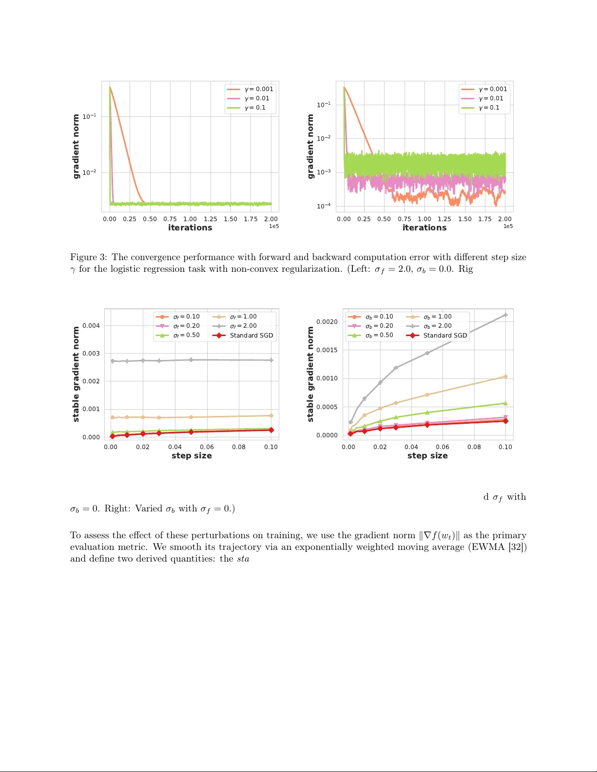
On the Con v ergence of Sto c hastic Gradien t Descen t with P erturb ed F orw ard-Bac kw ard P asses Boao K ong 1 ∗ kongboao@stu.pku.edu.cn Hengrui Zhang 2 ∗ 2022141210007@stu.scu.edu.cn Kun Y uan 1 † kunyuan@pku.edu.cn F ebruary 25, 2026 Abstract W e study stochastic gradien t descen t (SGD) for composite optimization problems with N sequen tial op erators sub ject to p erturbations in both the forward and bac kward passes. Unlike classical analyses that treat gradien t noise as additive and lo calized, p erturbations to intermediate outputs and gradients cascade through the computational graph, comp ounding geometrically with the n umber of op erators. W e present the ﬁrst comprehensive theoretical analysis of this setting. Sp eciﬁcally , w e c haracterize ho w forw ard and bac kward perturbations propagate and amplify within a single gradient step, deriv e conv ergence guarantees for b oth general non-conv ex ob jectiv es and functions satisfying the Poly ak–Ło jasiewicz condition, and iden tify conditions under which p erturbations do not deteriorate the asymptotic conv ergence order. As a b ypro duct, our analysis furnishes a theoretical explanation for the gradient spiking phenomenon widely observ ed in deep learning, precisely characterizing the conditions under which training recov ers from spik es or div erges. Exp erimen ts on logistic regression with conv ex and non-conv ex regularization v alidate our theories, illustrating the predicted spike behavior and the asymmetric sensitivity to forw ard v ersus bac kward p erturbations. Con ten ts 1 In tro duction 2 1.1 Motiv ating Examples . . . . . . . . . . . . . . . . . . . . . . . . . . . . . . . . . . . . . . . . . . . . . . 3 1.2 Sto c hastic Gradient Descent . . . . . . . . . . . . . . . . . . . . . . . . . . . . . . . . . . . . . . . . . . 3 1.3 SGD with P erturb ed F orw ard and Backw ard Passes . . . . . . . . . . . . . . . . . . . . . . . . . . . . 4 1.4 Op en Questions, Theoretical Challenges, and Contributions . . . . . . . . . . . . . . . . . . . . . . . . 5 1.4.1 Op en questions . . . . . . . . . . . . . . . . . . . . . . . . . . . . . . . . . . . . . . . . . . . . . 5 1.4.2 Theoretical challenges . . . . . . . . . . . . . . . . . . . . . . . . . . . . . . . . . . . . . . . . . 6 1.4.3 Con tributions . . . . . . . . . . . . . . . . . . . . . . . . . . . . . . . . . . . . . . . . . . . . . . 6 2 Related W orks 7 1 Peking Universit y . 2 Sich uan Univ ersity . ∗ Equal con tribution. † Corresponding author. 1 3 Preliminaries 8 3.1 Notations . . . . . . . . . . . . . . . . . . . . . . . . . . . . . . . . . . . . . . . . . . . . . . . . . . . . 8 3.2 Third-Order T ensor and Its Op erator Norm . . . . . . . . . . . . . . . . . . . . . . . . . . . . . . . . . 9 3.3 Assumptions . . . . . . . . . . . . . . . . . . . . . . . . . . . . . . . . . . . . . . . . . . . . . . . . . . 9 4 Error Propagation Analysis 10 5 Con vergence of SGD with P erturb ed F orw ard-Bac kward Passes 16 5.1 Con vergence with Non-Con vex Assumption . . . . . . . . . . . . . . . . . . . . . . . . . . . . . . . . . 16 5.2 Con vergence with PL Condition . . . . . . . . . . . . . . . . . . . . . . . . . . . . . . . . . . . . . . . . 17 5.3 In terpreting the Conv ergence Theorems . . . . . . . . . . . . . . . . . . . . . . . . . . . . . . . . . . . 18 6 Conditions Ensuring Conv ergence under P erturbations 19 6.1 Con vergence Conditions for F requen t Perturbation . . . . . . . . . . . . . . . . . . . . . . . . . . . . . 19 6.2 Con vergence Conditions for Intermitten t P erturbation . . . . . . . . . . . . . . . . . . . . . . . . . . . 20 6.3 Con vergence with Gradien t Spik es . . . . . . . . . . . . . . . . . . . . . . . . . . . . . . . . . . . . . . 23 7 Exp erimen ts 23 7.1 Exp erimen tal Setup . . . . . . . . . . . . . . . . . . . . . . . . . . . . . . . . . . . . . . . . . . . . . . 23 7.2 Exp erimen tal Results . . . . . . . . . . . . . . . . . . . . . . . . . . . . . . . . . . . . . . . . . . . . . . 25 7.2.1 Con vergence with frequen t zero-mean p erturbations . . . . . . . . . . . . . . . . . . . . . . . . 25 7.2.2 Con vergence with frequen t non-zero-mean computation perturbations . . . . . . . . . . . . . . 26 7.2.3 Con vergence with in termittent forward computation p erturbations . . . . . . . . . . . . . . . . 26 8 Conclusion and F uture W orks 27 A Counter examples 32 A.1 Zero-mean Noise can Lead to Biased Ev aluated Gradient . . . . . . . . . . . . . . . . . . . . . . . . . . 32 A.2 Non-con vergence Induced b y F requent O (1) Magnitude P erturbations in F orw ard Propagation . . . . . 32 A.3 Non-con vergence With T op-K Compressor . . . . . . . . . . . . . . . . . . . . . . . . . . . . . . . . . . 33 1 In tro duction This pap er inv estigates the following optimization problem with a comp osite ob jectiv e inv olving N ≥ 2 op erators: min w ∈ R d ℓ ( w ) := E x ∈D h L ( x ; w ) := F ( x ; w ) + R ( w ) i , (1a) s.t. F ( x ; w ) := y N , y i = f i ( y i − 1 , w i ) , ∀ i ∈ { 1 , . . . , N } , (1b) where eac h op erator f i : R d i − 1 × R d w i → R d i represen ts the i -th comp onen t of the comp osite function F ( x ; w ) , with y i ∈ R d i and w i ∈ R d w i . The global optimization v ariable is deﬁned as w := ( w ⊤ 1 , w ⊤ 2 , . . . , w ⊤ N ) ⊤ ∈ R d , where eac h w i corresp onds to operator f i , and the total dimension is d = d w 1 + d w 2 + · · · + d w N . Here, the term R ( w ) denotes a diﬀeren tiable regularizer used to preven t mo del ov erﬁtting. Quan tity x denotes a data sample dra wn from the distribution D , and y i represen ts the in termediate output of the i -th operator f i , with the initial condition y 0 = x ∈ R d 0 . 2 1.1 Motiv ating Examples The general formulation ( 1 ) arises in v arious scenarios in v olving sequential decision-making and operator-wise pro cessing. Several motiv ating examples are provided below. Example 1: Deep neural netw ork. A deep neural netw ork (DNN) is a prime example of the problem in ( 1 ) , where each op erator f i represen ts a neural netw ork lay er [ 11 ]. Each la yer transforms its input y i − 1 using learnable parameters w i to pro duce the output y i . The comp osite function F ( x ; w ) consists of these successiv e transformations, with the ﬁnal lay er generating the v alue of the loss function. The hierarchical structure and nonlinearity of DNNs allow them to mo del complex data relationships [ 30 ], making them particularly eﬀectiv e for tasks such as image recognition, natural language processing, and reinforcement learning [29, 55, 44]. Example 2: Finite horizon optimization. T raditional optimization seeks to ensure go od p erformance as the num b er of iterations T approac hes inﬁnit y [ 46 ]. In contrast, ﬁnite horizon optimization [ 63 ] is to iden tify optimal h yp erparameter sp eciﬁcally for a small and ﬁnite T . F or instance, to determine optimal learning rate sc hedules for gradien t descent o ver T iterations, we form ulate the problem [20]: min { γ 1 , ··· ,γ T } max g ∈G ε ( x T ) , (2a) s.t. x t = x t − 1 − γ t ∇ g ( x t − 1 ) , ∀ t ∈ { 1 , . . . , T } . (2b) Here, x T is obtained through T gradien t descen t steps with learning rate γ t at iteration t . F unction ε ( · ) ev aluates the p erformance of x T , and G denotes the ob jective function class. Problem ( 2 ) seeks optimal { γ 1 , . . . , γ T } to ac hieve the best p ossible p erformance after T iterations [ 27 ]. By setting w = { γ 1 , . . . , γ T } , y T +1 = max g ∈G ε ( x T ) , y t = x t for t ∈ { 1 , . . . , T } , y 0 = x 0 , f t ( y t − 1 , γ t ) = y t − 1 − γ t ∇ g ( y t − 1 ) , and F ( x ; w ) = y T +1 , problem ( 2 ) reduces to the deterministic v ersion of problem ( 1 ). Example 3: Linear quadratic con trol. The linear quadratic control (LQC) problem [ 36 , 4 ] addresses optimal con trol of linear systems. The goal is to ﬁnd a control p olicy based on observed information that minimizes the exp ected v alue of a quadratic cost function ov er a ﬁnite time horizon. The problem is given as follo ws: min π E " T − 1 X t =0  x ⊤ t Q x x t + u ⊤ t R u u t  + x ⊤ T Q T x T # , (3a) s.t. u t = π t ( x 0: t ; u 0: t − 1 ) , ∀ t ∈ { 0 , . . . , T − 1 } , (3b) x t +1 = Ax t + B u t , ∀ t ∈ { 0 , . . . , T − 1 } . (3c) Here, the state x t ev olves according to the linear combination of previous state x t − 1 and control input u t − 1 with co eﬃcien t matrices A and B . The p olicy π t generates control action u t based on the history of states x 0: t . Problem ( 3 ) seeks the optimal p olicy π = ( π 1 , . . . , π T − 1 ) to minimize the total exp ected cost, determined by w eighting matrices Q x , R u , and Q T . By setting w = π = ( π 1 , . . . , π T − 1 ) , y t = [ u t ; x t +1 ] , and f t ( y t − 1 , π t ) = [ π t ( x 0: t ; u 0: t − 1 ); Ax t + B u t ] , problem ( 3 ) reduces to ( 1 ). 1.2 Sto c hastic Gradien t Descen t Sto c hastic Gradien t Descen t (SGD) is a widely used optimization algorithm for solving the problem describ ed in ( 1 ) . Giv en the sequen tial nature of the op erators in this formulation, eac h iteration of SGD inv olves b oth forw ard and backw ard passes to compute the sto c hastic gradient. Let u i := ∇ w i F ( x ; w ) and v i := ∇ y i F ( x ; w ) denote the sto c hastic gradien ts with resp ect to weigh t w i and intermediate output y i , resp ectiv ely , where v N = 1 (since the output y N is the ﬁnal op erator’s result). W e also use r i := ∇ w i R ( w ) to denote the gradien t of R ( w ) with respect to w i . The SGD pro cedure for optimizing ( 1 ) is as follo ws: (F orward) y ( t ) i = f i ( y ( t ) i − 1 , w ( t ) i ) , i = 1 , 2 , . . . , N , (4a) (Bac kward) v ( t ) i − 1 = ∇ 1 f i ( y ( t ) i − 1 , w ( t ) i ) ⊤ v ( t ) i , i = N , N − 1 , . . . , 2 , (4b) 3 (Gradien t) u ( t ) i = ∇ 2 f i ( y ( t ) i − 1 , w ( t ) i ) ⊤ v ( t ) i , i = N , N − 1 , . . . , 1 , (4c) (Up date) w ( t +1) i = w ( t ) i − γ ( u ( t ) i + r ( t ) i ) , i = N , N − 1 , . . . , 1 . (4d) W e refer to y i , v i , u i , and w i as the interme diate output , interme diate gr adient , weight gr adient , and weight , resp ectiv ely . Algorithm ( 4 ) is structured in to four key stages: 1. F orw ard pass. The input x is propagated through all N op erators us ing ( 4a ) , where y ( t ) 0 = x . This step sequentially ev aluates all op erators. 2. Bac kward pass. Gradien t information is propagated in rev erse order. In termediate gradient v ( t ) i is computed at each op erator i starting from i = N do wn to i = 1 . Sp eciﬁcally , v ( t ) i − 1 is up dated by applying the chain rule ( 4b ) , where ∇ 1 f i ∈ R d i × d i − 1 is the Jacobian of the op erator f i with resp ect to y i − 1 . 3. Gradien t. The parameter gradien ts u ( t ) i are computed at each op erator by combining v ( t ) i with ∇ 2 f i ∈ R d i × d w i , the lo cal Jacobians of the op erators with resp ect to the weigh t w i , see the up date in ( 4c ). 4. W eigh t up date. The weigh ts w i are up dated with ( 4d ) , where γ is the learning rate, and the up date pro ceeds from i = N down to i = 1 . This iterativ e pro cedure minimizes the comp osite ob jective function F ( x ; w ) together with the regularizer R ( w ) b y up dating the op erator-wise parameters { w i } N i =1 using gradient information with resp ect to b oth in termediate outputs and mo del weigh ts. Note that R ( w ) dep ends only on w , so its gradien t r i = ∇ w i R ( w ) can b e computed and added directly in the up date step, without participating in the forward/bac kward passes for ev aluating F ( x ; w ) . 1.3 SGD with P erturb ed F orward and Backw ard Passes In practical implementations, gradient ev aluation is susceptible to p erturbations in b oth the forward and bac kward passes. T o mo del these eﬀects, w e introduce forward and bac kward p erturbation terms, δ ( t ) i and ε ( t ) i , for the i -th op erator at iteration t . W e model p erturbations only in the forw ard/backw ard ev aluation of the sample-dep enden t comp osite loss F ( x ; w ) ; the parameter-only regularizer R ( w ) is treated as exact and con tributes deterministically via r i = ∇ w i R ( w ) . Incorp orating these perturbations leads to an SGD up date with p erturbed forward and bac kward passes: (F orward) ˜ y ( t ) i = f i ( ˜ y ( t ) i − 1 , w ( t ) i ) + δ ( t ) i , i = 1 , 2 , · · · , N , (5a) (Bac kward) ˜ v ( t ) i − 1 = ∇ 1 f i ( ˜ y ( t ) i − 1 , w ( t ) i ) ⊤ ˜ v ( t ) i + ε ( t ) i , i = N , N − 1 , · · · , 2 , (5b) (Gradien t) ˜ u ( t ) i = ∇ 2 f i ( ˜ y ( t ) i − 1 , w ( t ) i ) ⊤ ˜ v ( t ) i , i = N , N − 1 , · · · , 1 , (5c) (Up date) w ( t +1) i = w ( t ) i − γ ( ˜ u ( t ) i + r ( t ) i ) , i = N , N − 1 , . . . , 1 . (5d) Here, ˜ y i and ˜ v i denote the corrupted intermediate output and intermediate gradien t, induced by (random) p erturbations δ i and ε i , resp ectiv ely . Since the weigh t gradient ˜ u i dep ends on the corrupted in termediate gradien t ˜ v i in ( 5c ), it yields a corrupted gradien t ˜ u i . Figure 1 illustrates algorithm pro cedure listed in ( 5 ). The p erturbed SGD framew ork ( 5 ) naturally emerges in numerous practical scenarios. F or instance, mixed- precision training [ 42 , 8 , 43 , 23 , 15 , 54 , 14 ], widely adopted for DNN, combines lo w-precision computations (FP16/INT8) with FP32 mo del weigh ts to reduce memory consumption and accelerate training on sp ecialized hardw are. This precision reduction inherently introduces systematic perturbations: forward passes in lo wer precision generate rounding errors ( δ i ), while reduced-precision in termediate gradient computations yield bac kward p erturbations ( ε i ). Si milarly , pipeline-parallel DNN training partitions neural netw ork 4 operator 1 operator 2 operator 3 operator N data loss interme diate output interme diate gradien t no pertu rbation: forward -backward pe rturbation: stochast ic optimiz ation with co mposite operato rs Figure 1: An illustration of SGD algorithm with perturb ed forward and bac kward passes. la yers across m ultiple devices, requiring communication of in termediate outputs and gradien ts. T o mitigate comm unication ov erhead, these v ariables undergo compression b efore transmission [ 21 , 24 , 56 , 38 ], inducing forw ard and backw ard p erturbations at operator boundaries; see App endix A.3 for a simple tw o-lay er example where a deterministic T op-1 compressor prev en ts con vergence even though the uncompressed metho d conv erges. A dditionally , hardware-induced errors—such as bit ﬂips from cosmic rays or voltage instabilit y [ 49 , 26 , 19 ]—in tro duce unpredictable computational p erturbations during forward and bac kward passes. F urthermore, in the LQC problem ( 3 ) , the state x t ma y b e aﬀected by random Gaussian noise, e.g., x t +1 = Ax t + B u t + δ t , where δ t ∼ N (0 , Σ δ ) . These diverse sources of p erturbations demonstrate that SGD with p erturbed forward and bac kward passes captures the fundamen tal dynamics of mo dern optimization, where exact gradients ma y not alwa ys b e feasible. 1.4 Op en Questions, Theoretical Challenges, and Con tributions 1.4.1 Open questions Despite the widespread use of SGD with perturb ed forw ard and backw ard passes in mo dern optimization and mac hine learning, our theoretical understanding remains limited. Most existing literature fo cuses exclusively on noise or p erturbations to w eight gradients u i in ( 5c ) , where errors remain localized—they neither propagate forw ard through subsequent op erators nor backw ard through intermediate gradien ts, aﬀecting only the mo del w eight update. In contrast, perturbations to intermediate outputs y i in ( 5a ) and in termediate gradients v i in ( 5b ) cascade through the computational graph, accumulating across operators to create compounded errors that fundamentally complicate con vergence analysis. This pap er inv estigates the following three fundamen tal op en questions: Q1 . (Error dynamics) Ho w can the propagation and accum ulation of comp ounded errors through the forw ard and bac kward passes be theoretically c haracterized? Q2. (Con vergence) Can SGD con verge to optimal solutions under p erturbed forward and bac kward passes, and how do these p erturbations quan titatively impact the con vergence behavior? Q3. (Robustness) Under what conditions do p erturbations not aﬀect conv ergence rates, and what prop erties of p erturbations con tribute to this robustness? 5 1.4.2 Theoretical challenges The main challenge arises from compounded error propagation through computational graphs. Standard SGD analyses [ 9 ] treat gradient errors as additive noise that is indep enden t of computation—mo deling p erturbed gradients as ˜ u = ∇ f ( w ) + ε with exogenous ε . In contrast, framew ork ( 5 ) generates p erturbations endogenously that cascade through operators, creating complex inter-operator dep endencies. Consider a linear neural netw ork with f i ( y i − 1 , W i ) = W i y i − 1 , zero forward p erturbations ( δ ( t ) i = 0 ), and constant bac kward p erturbations ( ε ( t ) i = ε i ). The w eight gradien t ˜ u 1 under b oth models rev eals the distinction: (A dd. p erturbation) ˜ u 1 = W ⊤ 2 · · · W ⊤ N v N · v ⊤ 1 + ε, (6a) (A cc. p erturbation) ˜ u 1 =  W ⊤ 2  · · ·  W ⊤ N v N + ε N  + · · ·  + ε 2  v ⊤ 1 + ε 1 . (6b) Here, ˜ u 1 denotes the p erturb ed gradient with resp ect to W 1 , while “Add.” and “Acc.” denote additive and accum ulative perturbations, resp ectiv ely . The perturb ed formulation ( 6b ) exhibits three pathological b eha viors absent from standard SGD analyses with additive noise: (1) Geometric error ampliﬁcation. The deep est perturbation ε N is multiplied by the matrix pro duct W ⊤ 1 · · · W ⊤ N − 1 , p oten tially causing exp onen tial gro wth with netw ork depth—a phenomenon that can trigger conv ergence failure. (2) Cascading error in terference. The nested structure creates nonlinear in teractions b et ween op erator-wise p erturbations, where errors comp ound in wa ys that simple noise mo dels cannot capture. (3) Biased gradien t estimates. Ev en when p erturbations δ ( t ) i and ε ( t ) i ha ve zero exp ectation, the nonlinear op erators in ( 5 ) induce bias suc h that E [ ∇ 2 f i ( ˜ y ( t ) i − 1 , w ( t ) i )]  = ∇ 2 f i ( y ( t ) i − 1 , w ( t ) i ) . These eﬀects critically challenge analysis, requiring new theoretical frameworks b eyond classical SGD theory . 1.4.3 Con tributions This pap er pro vides the ﬁrst comprehensive analysis for SGD under p erturb ed forw ard and bac kward passes. Our contributions are: C1. W e theoretically characterize the propagation of forw ard and backw ard p erturbations within a single gradien t step, demonstrating that these p erturbations amplify exp onen tially with the n um b er of op erators, whic h addresses Q1. C2. W e establish conv ergence guarantees for p erturbed SGD on b oth general non-conv ex functions and those satisfying the P olyak–Ło jasiewicz (PL) condition. By explicitly quantifying the impact of forward and backw ard errors on the conv ergence rate, w e address open question Q2. C3. W e identify the sp eciﬁc conditions under whic h forward and backw ard p erturbations do not deteriorate the asymptotic order of the conv ergence rate, directly addressing op en question Q3. As a side result, our analysis provides an explanation for the “gradient spiking” phenomenon commonly observ ed in deep learning. These spik es are sudden, temp orary jumps in the gradient, often triggered by p erturbations during the forward and bac kward passes. While some spik es are reco verable, meaning they can b e corrected during the training pro cess, others can lead to training divergence, see Figure 2 for the illustration. Our theoretical analysis of the p erturbed SGD ( 5 ) clearly establishes the conditions under which the optimization can recov er or exp erience a complete crash. Organization. This pap er is organized as follows: Section 2 presents related work. Section 3 presents preliminaries, including notations and assumptions. Section 4 analyzes the propagation of forward and bac kward computation errors. Section 5 derives the conv ergence rate of the SGD algorithm with computation error under non-smo oth settings and PL conditions. Section 6 establishes conditions on computation error that guaran tee conv ergence and enable recov ery from gradient spikes. Section 7 presents n umerical exp erimen ts v alidating our theoretical ﬁndings. Finally , Section 8 concludes the pap er. 6 0 200 400 600 800 1000 1200 1400 iteration 0.0 0.5 1.0 1.5 2.0 2.5 gradient norm Gradient Stability Analysis SGD without spike SGD with spike (convergence) SGD with spike (non-convergence) 0 200 400 600 800 1000 1200 1400 iteration 0.0 0.2 0.4 0.6 0.8 1.0 1.2 1.4 loss Loss Convergence Analysis SGD without spike SGD with spike (convergence) SGD with spike (non-convergence) Figure 2: Comparison of gradien t spike patterns leading to contrasting outcomes. The gradient norm (left) and loss (right) tra jectories illustrate tw o scenarios: a large-magnitude spik e (orange) that p ermits rapid reco very and con vergence, versus a more mo derate spik e (blue) that triggers persistent deviation and even tual non-con vergence. 2 Related W orks Our analysis builds up on and extends several lines of theoretical work on optimization algorithms sub ject to computational inaccuracies. Algorithms with inexact gradien t oracles. The eﬀect of computational inaccuracy on gradient methods has b een studied extensiv ely under inexact ﬁrst-order oracle mo dels, in which the algorithm accesses a p erturbed gradient at each iteration. Classical results analyze gradient descent with deterministic errors (e.g., ﬁnite diﬀerences in zeroth-order metho ds, early termination of inner solvers, discretization errors in PDE-constrained optimization, and surrogate mo del appro ximations) and deriv e con vergence and complexit y guaran tees that degrade gracefully with the error level [ 7 , 18 , 17 ]. In stochastic settings, the gradien t is t ypically corrupted by additive sampling noise from random data sampling; related analyses quantify the con vergence p erformance t ypically under conditional moment or b ounded-v ariance assumptions [ 25 , 52 , 9 ]. A parallel line of work examines inexact proximal p oint and proximal-gradien t metho ds, in which proximal subproblems are solv ed appro ximately while still ensuring descent and conv ergence [ 31 , 10 , 51 , 28 ]. More recen t developmen ts reﬁne oracle mo dels for comp osite structures and higher-order inexactness, and establish non-asymptotic b ounds that explicitly trac k oracle accuracy [53, 3, 45]. Man y pre-training approaches for large language mo dels can b e view ed as ﬁrst-order metho ds with inexact gradien ts due to communication or computation errors. Examples include gradien t quantization and sparsiﬁ- cation [ 2 , 50 , 22 ], mixed-precision training [ 42 , 43 , 40 ], and gradient clipping [ 37 , 48 ]. The analysis typically treats the gradien t as a perturbation of the ideal sto c hastic gradien t and relates conv ergence to error statistics (bias, v ariance, or relativ e b ounds). This persp ective is particularly p o werful when the p erturbation can be mo deled as an additive err or to the computed gradient, as illustrated i n ( 6a ) , enabling standard descent and martingale analyses. The perturbation mechanism in ( 5 ) diﬀers fundamen tally from standard inexact-oracle models. Perturbations are injected within the forward–bac kward pass at in termediate activ ations and adjoin ts, propagating through the computational graph b efore the gradient forms. The resulting error is endogenous, shap ed by lo cal Jacobians at the current iterate, creating inter-operator dependencies. Moreov er, ev en zero-mean p erturbations can induce gradien t bias due to the comp osite structure; see App endix A.1 for a simple scalar example. These considerations motiv ate our analysis of SGD with p erturb ed forw ard–backw ard passes. Sto c hastic compositional optimization (SCO). Stochastic comp ositional optimization [ 58 , 57 , 16 ] studies problems with nested exp ectation structure, such as min w ∈ R d F ( w ) := E ζ  f ζ  G ( w )  , G ( w ) := E ξ [ g ξ ( w )] , (7) 7 and their multi-lev el generalizations [ 61 , 6 , 62 , 64 , 33 , 34 ] (see also constrained or pro jection-free v ariants [ 59 , 35 ]). A k ey diﬃculty is that computing ∇ F ( w ) requires ev aluating the deriv ative at G ( w ) , an inner exp ectation that is not observ able from a single sample ξ . Practical metho ds thus maintain auxiliary v ariables (typically one per level) to track the nested expectations and form quasi-gradients b y combining comp onen t deriv ative estimates with these track ed quantities. Since the outer deriv ativ e emplo ys an evolving appro ximation instead of the exact inner exp ectations, the descent directions b ecome biased. Consequently , the analysis fo cuses on con trolling the coupled iterate-trac king dynamics through m ulti-timescale step sizes or single-lo op trac king/v ariance-reduction designs. Our setting diﬀers from SCO in b oth form ulation and error mec hanism. At a high level, b oth SCO and our framew ork in volv e comp ositional graphs where intermediate quantities are accessed inexactly , leading to biased gradien t surrogates. How ever, the source and nature of inexactness are fundamentally diﬀeren t. In SCO, inexactness arises from estimating inner exp e ctations within each operator; this bias can b e reduced algorithmically by allocating more computational eﬀort to inner estimation or tracking—for example, using larger inner batc hes or more accurate v ariance-reduced estimators. In con trast, our setting ( 5 ) in volv es a single exp ectation, where inexactness stems from perturbations within the forward and backw ard passes themselv es. Crucially , increasing batch size reduces sampling v ariance but do es not diminish these within- pass p erturbations, whic h p ersist independently of sample size. Moreov er, p erturbations in our setting are depth-coupled: they propagate and accumulate along sample paths through the computational graph. This cen tral challenge—depth-wise propagation and accumulation of intermediate disturbances—lies beyond the scop e of existing SCO analyses [58, 57, 16, 61, 6]. A Q-SGD. The most closely related work is AQ-SGD, whic h analyzes activ ation quantization for distributed pip eline training [ 56 ]. Critically , AQ-SGD is tailored to pip eline parallelism with communication-induced p erturbations and do es not address general forward-bac kward p erturbation mechanisms or pro vide the depth-wise error propagation and disturbance-frequency analysis dev elop ed here. 3 Preliminaries This section introduces necessary notations and assumptions. 3.1 Notations W e denote the gradient of ℓ ( w ) b y ∇ ℓ ( w ) ∈ R d . F or i = 1 , . . . , N , the partial deriv ativ e of ℓ ( w ) with resp ect to parameter w i is denoted b y ∇ i ℓ ( w ) := ∂ ℓ ( w ) ∂ w i ∈ R d w i . F or eac h op erator f i ( y i − 1 , w i ) : R d i − 1 × R d w i → R d i , the Jacobian matrices with resp ect to the input y i − 1 and parameter w i are denoted b y ∇ 1 f i ( y i − 1 , w i ) ∈ R d i × d i − 1 and ∇ 2 f i ( y i − 1 , w i ) ∈ R d i × d w i , resp ectively . W e also denote ∇ 2 21 f i ( y i − 1 , w i ) ∈ R d i × d w i × d i − 1 as the partial deriv ative of ∇ 2 f i ( y i − 1 , w i ) with resp ect to y i − 1 . W e use ∥ · ∥ to denote the Euclidean norm for vectors and F rob enius norm for matrices and tensors, and ∥ · ∥ op to denote the induced op erator norm. Throughout the pap er, sup erscripts t indicate the iteration index, while subscripts i denote the comp onen t index. F or any family of comp onen t-wise vectors { a i } N i =1 (e.g., u i , v i , r i and their p erturb ed coun terparts), we use b oldface a := ( a ⊤ 1 , . . . , a ⊤ N ) ⊤ to denote the stac ked/concatenated v ector across comp onen ts (and similarly ˜ a for the p erturbed v ersion). W e deﬁne the minimum ob jectiv e v alue as ℓ ∗ := min w ℓ ( w ) and the initial optimality gap as ∆ 0 := ℓ ( w (0) ) − ℓ ∗ . The notation a ≲ b means a ≤ C b for some constan t C > 0 indep enden t of problem parameters. Notation ˜ O ( · ) hides logarithmic depe ndence on T . F or the sto c hastic setting, let F ( t ) denote the ﬁltration generated up to iteration t , with E t [ · ] denoting the conditional exp ectation given F ( t ) . F urthermore, let G ( t ) i = σ ( F ( t ) ∪ { ˜ y ( t ) 1 , . . . , ˜ y ( t ) i } ) denote the ﬁltration generated by perturb ed outputs up to op erator i in the forward pass, and let H ( t ) i = σ ( G ( t ) N ∪ { ˜ v ( t ) N , . . . , ˜ v ( t ) i } ) denote the ﬁltration generated by the full forward pass and backw ard gradients from op erator N do wn to op erator i . W e use E G i t [ · ] and E H i t [ · ] to denote conditional exp ectations with resp ect to G ( t ) i and H ( t ) i , resp ectiv ely . 8 3.2 Third-Order T ensor and Its Op erator Norm W e deﬁne multiplication b et w een third-order tensors and matrices, along with the induced op erator norm. Let H := ( H j αβ ) ∈ R p × m × n b e a third-order tensor and A := ( A αβ ) ∈ R m × n b e a matrix. The product H ( A ) ∈ R p is given by con tracting ov er the last tw o indices: [ H ( A )] j := m X α =1 n X β =1 H j αβ A αβ , j = 1 , . . . , p. (8) That is, for eac h j , the comp onent [ H ( A )] j equals P α,β H j αβ A αβ . F rom ( 8 ) , we deﬁne the op erator norm of H as ∥H∥ op := sup A ∈ R m × n , A  =0 ∥H ( A ) ∥ 2 ∥ A ∥ = sup ∥ A ∥ =1 ∥H ( A ) ∥ 2 . (9) In tuitively , ∥H∥ op measures the largest ampliﬁcation of the output norm ∥H ( A ) ∥ 2 when the input matrix A has unit F rob enius norm. The F rob enius norm of H can b e expressed as ∥H∥ :=  X j,α,β H 2 j,α,β  1 2 . (10) 3.3 Assumptions The following tw o assumptions are standard in the conv ergence analysis of sto c hastic gradient algorithms. Assumption 1 ( Smoothness of the loss function) . Ther e exists a c onstant L ∇ ℓ > 0 such that ∇ ℓ ( w ) is L ∇ ℓ -Lipschitz c ontinuous. Assumption 2 ( Stochasticity) . Ther e exists a c onstant σ > 0 such that for any given x ∈ R d 0 , the unp erturb e d gr adient or acles satisfy: E x ∈D [ ∇ w L ( x ; w )] = ∇ ℓ ( w ); E x ∈D h ∥∇ w L ( x ; w ) − ∇ ℓ ( w ) ∥ 2 i ≤ σ 2 . W e also make the following assumption on the smo othness of eac h op erator. Assumption 3 ( Opera tor smoothness) . F or e ach i = 1 , . . . , N , ther e exist c onstants C ∇ f , C ∇ 2 f , L f , L ∇ f , L ∇ 2 f > 0 such that for al l y i − 1 ∈ R d i − 1 and w i ∈ R d w i : 1. The Jac obians satisfy ∥∇ j f i ( y i − 1 , w i ) ∥ op ≤ C ∇ f ( j = 1 , 2) , ∥∇ 2 21 f i ( y i − 1 , w i ) ∥ op ≤ C ∇ 2 f . 2. The op er ator f i is Lipschitz c ontinuous with r esp e ct to y i − 1 with c onstant L f . Her e, Lipschitz c ontinuity of f i is me asur e d in the Euclide an norm. 3. The mappings ∇ f i , and ∇ 2 f i ar e Lipschitz c ontinuous with r esp e ct to b oth y i − 1 and w i , with c onstants L ∇ f , and L ∇ 2 f , r esp e ctively. Her e, Lipschitz c ontinuity of ∇ f i and ∇ 2 f i is me asur e d in the F r ob enius norm. Assumption 3 is an op erator-regularit y condition that controls how perturbations amplify through the computational graph during the forw ard and backw ard passes. Bounded-Jacobian and Lipschitz-t yp e conditions are standard in analyses inv olving intermediate perturbations; see, e.g., [13, 56, 38, 41, 12]. † † When the component mappings are t wice diﬀerentiable, the Lipsc hitz requirements on the deriv ative maps in Assumption 3 can be interpreted as b ounded v ariation of the local Jacobians, or equiv alently , b ounded mixed second-order deriv atives. 9 W e emphasize that Assumption 3 is not an algorithmic constraint: throughout the pap er we analyze the plain SGD up date in ( 5d ) without pro jection or clipping. That said, Assumption 3 can b e in terpreted lo c al ly : it suﬃces for the stated regularity b ounds to hold on a compact region containing the iterates and intermediate states visited during training. Such compactness can arise, for example, from ﬁnite data combined with b ounded parameter regimes, explicit pro jection to a compact set, or standard clipping/normalization practices. Our goal is to isolate the eﬀect of forward/bac kward p erturbations; incorporating suc h safeguards would only strengthen stabilit y in practice. Finally , we mak e the following assumption of the Poly ak-Ło jasiewicz (PL) condition [47] for ℓ ( w ) : Assumption 4 (PL condition) . Ther e exist a c onstant µ > 0 such that for any w ∈ R d , it holds that ∥∇ ℓ ( w ) ∥ 2 ≥ 2 µ ( ℓ ( w ) − ℓ ∗ ) . (11) The PL condition can b e implied b y strong con vexit y . In particular, adding an ℓ 2 regularizer R ( w ) = λ 2 ∥ w ∥ 2 mak es the loss ℓ ( w ) λ -strongly con vex whenev er the data-ﬁtting term is conv ex, which in turn ensures the PL inequality holds with µ = λ . 4 Error Propagation Analysis This section c haracterizes the propagation of forward and bac kward perturbations within a single gradient step. W e b egin with the following useful lemma. Lemma 1. Under Assumption 3 , ther e exists a c onstant C 2 v ≥ 1 such that ∥ v ( t ) i ∥ 2 ≤ C 2 v for al l t = 1 , 2 , . . . , T and i = 1 , 2 , . . . , N . Pr o of. F or i = 1 , 2 , . . . , N − 1 , the vector v ( t ) i can b e expressed as v ( t ) i =  ∇ 1 f N ( y ( t ) N − 1 , w ( t ) N )  ⊤ · · ·  ∇ 1 f i +2 ( y ( t ) i +1 , w ( t ) i +2 )  ⊤ ·  ∇ 1 f i +1 ( y ( t ) i , w ( t ) i +1 )  ⊤ . This yields the upp er b ound    v ( t ) i    2 ≤ N Y k = i +1    ∇ 1 f k ( y ( t ) k − 1 , w ( t ) k )    2 op ≤ C 2( N − i ) ∇ f , (12) where the ﬁrst inequality holds b ecause ∇ 1 f N ( y ( t ) N − 1 , w ( t ) N ) has dimension d N − 1 , so its op erator norm equals its Euclidean norm. Since N is a ﬁxed constan t and v ( t ) N = 1 , taking C v = max { 1 , C N ∇ f } ensures that ∥ v ( t ) i ∥ 2 ≤ C 2 v for all t = 1 , 2 , . . . , T and i = 1 , 2 , . . . , N . Lemma 1 ensures that the in termediate backw ard gradients v ( t ) i remain uniformly b ounded across all op erators and iterations. Th is controls ho w p erturbations introduced during the backw ard pass are ampliﬁed as they propagate tow ard earlier op erators. The b ound C v = max { 1 , C N ∇ f } reﬂects worst-case accumulation of Jacobian norms across the netw ork depth. The following theorem presents an upper b ound of the ℓ 2 -error term: Theorem 1. Supp ose Assumption 3 holds, then for i = 1 , 2 , · · · , N − 1 , ther e exist c onstants C e δ i , C e ε i +1 ≥ 0 , which ar e deﬁne d in ( 21 ) , such that: E  ∥ ˜ u ( t ) − u ( t ) ∥ 2  ≤ N − 1 X i =1 C e δ i E  ∥ δ ( t ) i ∥ 2  + N − 1 X i =1 C e ε i +1 E  ∥ ε ( t ) i +1 ∥ 2  , (13) holds for al l t = 1 , 2 , · · · , T . 10 Pr o of. W e ﬁrst consider the gradient ev aluation at the last comp onen t. W e hav e E     ˜ u ( t ) N − u ( t ) N    2  = E     ∇ 2 f N ( ˜ y ( t ) N − 1 , w ( t ) N ) − ∇ 2 f N ( y ( t ) N − 1 , w ( t ) N )    2  ≤ L 2 ∇ f E     ˜ y ( t ) N − 1 − y ( t ) N − 1    2  ≤ 2 C 2 v L 2 ∇ 2 f E     ˜ y ( t ) N − 1 − y ( t ) N − 1    2  , (14) where the inequality follo ws from the smo othness of ∇ 2 f N and the fact that C 2 v ≥ 1 . F or i = 1 , 2 , . . . , N − 1 , w e hav e E     ˜ u ( t ) i − u ( t ) i    2  = E     ∇ 2 f i ( ˜ y ( t ) i − 1 , w ( t ) i ) ⊤ ˜ v ( t ) i − ∇ 2 f i ( y ( t ) i − 1 , w ( t ) i ) ⊤ v ( t ) i    2  ≤ 2 E     ∇ 2 f i ( ˜ y ( t ) i − 1 , w ( t ) i )    2 op    ˜ v ( t ) i − v ( t ) i    2  + 2 E     ∇ 2 f i ( ˜ y ( t ) i − 1 , w ( t ) i ) − ∇ 2 f i ( y ( t ) i − 1 , w ( t ) i )    2 op    v ( t ) i    2  ≤ 2 C 2 ∇ f E     ˜ v ( t ) i − v ( t ) i    2  + 2 C 2 v L 2 ∇ f E     ˜ y ( t ) i − 1 − y ( t ) i − 1    2  , (15) where the second inequality follo ws from the smo othness of ∇ 2 f i together with the b oundedness of v ( t ) i and ∇ 2 f i . Summing o ver i = 1 , 2 , . . . , N yields E     ˜ u ( t ) − u ( t )    2  = N X i =1 E     ˜ u ( t ) i − u ( t ) i    2  ≤ 2 C 2 ∇ f N − 1 X i =1 E     ˜ v ( t ) i − v ( t ) i    2  + 2 C 2 v L 2 ∇ f N − 1 X i =1 E     ˜ y ( t ) i − y ( t ) i    2  . (16) In view of ( 16 ), we next analyze the error b et ween ˜ v ( t ) i and v ( t ) i for i = 1 , 2 , . . . , N − 1 . W e obtain E     ˜ v ( t ) i − v ( t ) i    2  = E     ∇ 1 f i +1 ( ˜ y ( t ) i , w ( t ) i +1 ) ⊤ ˜ v ( t ) i +1 − ∇ 1 f i +1 ( y ( t ) i , w ( t ) i +1 ) ⊤ v ( t ) i +1 + ε ( t ) i +1    2  ≤ 3 C 2 ∇ f E     ˜ v ( t ) i +1 − v ( t ) i +1    2  + 3 C 2 v L 2 ∇ f E     ˜ y ( t ) i − y ( t ) i    2  + 3 E     ε ( t ) i +1    2  ≤ · · · ≤ 3 C 2 v L 2 ∇ f N − 1 X j = i (3 C 2 ∇ f ) j − i E     ˜ y ( t ) j − y ( t ) j    2  + 3 N − 1 X j = i (3 C 2 ∇ f ) j − i E     ε ( t ) j +1    2  . (17) Finally , we bound the error b et ween ˜ y ( t ) i and y ( t ) i for i = 1 , 2 , . . . , N − 1 : E     ˜ y ( t ) i − y ( t ) i    2  = E     f i ( ˜ y ( t ) i − 1 , w ( t ) i ) − f i ( y ( t ) i − 1 , w ( t ) i ) + δ ( t ) i    2  ≤ 2 L 2 f E     ˜ y ( t ) i − 1 − y ( t ) i − 1    2  + 2 E     δ ( t ) i    2  ≤ · · · ≤ 2 i X j =1 (2 L 2 f ) i − j E     δ ( t ) j    2  . (18) 11 Substituting ( 17 ) into ( 16 ), we obtain E     ˜ u ( t ) − u ( t )    2  ≤ 6 C 2 ∇ f C 2 v L 2 ∇ f N − 1 X i =1 N − 1 X j = i (3 C 2 ∇ f ) j − i E     ˜ y ( t ) j − y ( t ) j    2  + 2 C 2 v L 2 ∇ f N − 1 X i =1 E     ˜ y ( t ) i − y ( t ) i    2  + 6 C 2 ∇ f N − 1 X i =1 N − 1 X j = i (3 C 2 ∇ f ) j − i E     ε ( t ) j +1    2  =2 C 2 v L 2 ∇ f N − 1 X i =1   i X j =0 (3 C 2 ∇ f ) j   E     ˜ y ( t ) i − y ( t ) i    2  + 2 N − 1 X i =1   i X j =1 (3 C 2 ∇ f ) j   E     ε ( t ) i +1    2  . (19) Substituting ( 18 ) into ( 19 ) then gives E     ˜ u ( t ) − u ( t )    2  ≤ 4 C 2 v L 2 ∇ f N − 1 X i =1   N − 1 X j = i " j X k =0 (3 C 2 ∇ f ) k # (2 L 2 f ) j − i   E     δ ( t ) i    2  + N − 1 X i =1   i X j =1 (3 C 2 ∇ f ) j   E     ε ( t ) i +1    2  . (20) Deﬁning C e δ i := 4 C 2 v L 2 ∇ f N − 1 X j = i " j X k =0 (3 C 2 ∇ f ) k # (2 L 2 f ) j − i , C e ε i +1 := i X j =1 (3 C 2 ∇ f ) j , (21) w e conclude that ( 13 ) holds for all t = 1 , 2 , . . . , T . Inequalit y ( 13 ) sho ws that the ℓ 2 error in the stochastic gradient due to forward and bac kward perturbations is con trolled by the ℓ 2 magnitudes of δ and ε . Crucially , the co eﬃcien ts C e δ i and C e ε i +1 scale exp onen tially with the depth of the computational graph, reﬂecting e O ( N ) error ampliﬁcation. This exp onen tial dependence illustrates how small p erturbations at individual op erators can comp ound in to signiﬁcant gradien t distortions as they propagate through the netw ork. W e next b ound the second moment of the bias with the following lemma. Lemma 2. Under Assumption 3 , it holds for i = 1 , 2 , · · · , N that:    E G i − 1 t [ ∇ 2 f i ( ˜ y ( t ) i − 1 , w ( t ) i ) − ∇ 2 f i ( y ( t ) i − 1 , w ( t ) i )]    2 ≤ 2 C 2 ∇ 2 f    E G i − 1 t [ ˜ y ( t ) i − 1 − y ( t ) i − 1 ]    2 + L 2 ∇ 2 f E G i − 1 t     ˜ y ( t ) i − 1 − y ( t ) i − 1    4  . (22) Pr o of. Since f is diﬀerentiable, we ha ve    E G i − 1 t [ ∇ 2 f i ( ˜ y ( t ) i − 1 , w ( t ) i ) − ∇ 2 f i ( y ( t ) i − 1 , w ( t ) i )]    2 =     E G i − 1 t  Z 1 0 ∇ 21 f i ( y ( t ) i − 1 + t ( ˜ y ( t ) i − 1 − y ( t ) i − 1 ) , w ( t ) i )  ˜ y ( t ) i − 1 − y ( t ) i − 1  dt      2 ≤ 2    ∇ 21 f i ( y ( t ) i − 1 , w ( t ) i ) E G i − 1 t [ ˜ y ( t ) i − 1 − y ( t ) i − 1 ]    2 +2     E G i − 1 t  Z 1 0  ∇ 21 f i ( y ( t ) i − 1 + t ( ˜ y ( t ) i − 1 − y ( t ) i − 1 ) , w ( t ) i ) − ∇ 21 f i ( y ( t ) i − 1 , w ( t ) i )  ( ˜ y ( t ) i − 1 − y ( t ) i − 1 ) dt      2 ≤ 2 C 2 ∇ 2 f    E G i − 1 t [ ˜ y ( t ) i − 1 − y ( t ) i − 1 ]    2 + L 2 ∇ 2 f E G i − 1 t     ˜ y ( t ) i − 1 − y ( t ) i − 1    4  , 12 whic h completes the pro of. Lemma 2 bounds the second moment of the bias introduced by forward p erturbations. Sp eciﬁcally , the squared deviation of the conditional exp ected gradient is con trolled by t wo terms: the squared norm of the exp ected forw ard error E G i − 1 t [ ˜ y ( t ) i − 1 − y ( t ) i − 1 ] and the fourth moment of the forward error ˜ y ( t ) i − 1 − y ( t ) i − 1 . Building on this result, we deriv e an upp er b ound for the second moment of the o verall bias as follo ws. Theorem 2. Supp ose Assumption 3 holds. Then for i = 1 , 2 , . . . , N − 1 , ther e exist c onstants C b δ i , ˜ C b δ i , C b ε i +1 ≥ 0 , which ar e deﬁne d in ( 33 ) , such that E     E t [ ˜ u ( t ) − u ( t ) ]    2  ≤ N − 1 X i =1 C b δ i E     E G i t [ δ ( t ) i ]    2  + N − 1 X i =1 ˜ C b δ i E     δ ( t ) i    4  + N − 1 X i =1 C b ε i +1 E     E H i +1 t [ ε ( t ) i +1 ]    2  (23) holds for al l t = 1 , 2 , . . . , T . Pr o of. W e ﬁrst consider the gradient ev aluation at the last comp onen t. By ( 22 ), we ha ve E     E t [ ˜ u ( t ) N − u ( t ) N ]    2  = E     E t [ ∇ 2 f N ( ˜ y ( t ) N − 1 , w ( t ) N ) − ∇ 2 f N ( y ( t ) N − 1 , w ( t ) N )]    2  ≤ 4 C 2 v C 2 ∇ 2 f E     E G N − 1 t [ ˜ y ( t ) N − 1 − y ( t ) N − 1 ]    2  + 2 C 2 v L 2 ∇ 2 f E     ˜ y ( t ) N − 1 − y ( t ) N − 1    4  . (24) F or i = 1 , 2 , . . . , N − 1 , we ha ve E     E t [ ˜ u ( t ) i − u ( t ) i ]    2  = E     E t h ∇ 2 f i ( ˜ y ( t ) i − 1 , w ( t ) i ) ⊤ ˜ v ( t ) i − ∇ 2 f i ( y ( t ) i − 1 , w ( t ) i ) ⊤ v ( t ) i i    2  ≤ 2 E     E t h ∇ 2 f i ( ˜ y ( t ) i − 1 , w ( t ) i ) ⊤  ˜ v ( t ) i − v ( t ) i i    2  + 2 E "     E t h ∇ 2 f i ( ˜ y ( t ) i − 1 , w ( t ) i ) − ∇ 2 f i ( y ( t ) i − 1 , w ( t ) i ) i ⊤ v ( t ) i     2 # . (25) Using the b oundedness of v ( t ) i and the fact that    E t h ∇ 2 f i ( ˜ y ( t ) i − 1 , w ( t ) i ) ⊤  ˜ v ( t ) i − v ( t ) i i    2 =    E t h ∇ 2 f i ( ˜ y ( t ) i − 1 , w ( t ) i ) ⊤ E H i t [ ˜ v ( t ) i − v ( t ) i ] i    2 ≤ E t     ∇ 2 f i ( ˜ y ( t ) i − 1 , w ( t ) i ) ⊤ E H i t [ ˜ v ( t ) i − v ( t ) i ]    2  = E t     ∇ 2 f i ( ˜ y ( t ) i − 1 , w ( t ) i )    2    E H i t [ ˜ v ( t ) i − v ( t ) i ]    2  (whic h follows from F ( t ) ⊂ H ( t ) i ), we obtain E     E t [ ˜ u ( t ) i − u ( t ) i ]    2  ≤ 2 E     ∇ 2 f i ( ˜ y ( t ) i − 1 , w ( t ) i )    2    E H i t [ ˜ v ( t ) i − v ( t ) i ]    2  + 2 C 2 v E     E t h ∇ 2 f i ( ˜ y ( t ) i − 1 , w ( t ) i ) − ∇ 2 f i ( y ( t ) i − 1 , w ( t ) i ) i    2  ≤ 2 C 2 ∇ f E     E H i t [ ˜ v ( t ) i − v ( t ) i ]    2  + 4 C 2 v C 2 ∇ 2 f E     E G i − 1 t [ ˜ y ( t ) i − 1 − y ( t ) i − 1 ]    2  + 2 C 2 v L 2 ∇ 2 f E     ˜ y ( t ) i − 1 − y ( t ) i − 1    4  . (26) 13 where the last inequality follows from the boundedness of ∇ f i , Lemma 2 , and the inclusion F ( t ) ⊂ G ( t ) i − 1 . Summing ov er i = 1 , 2 , . . . , N yields E     E t [ ˜ u ( t ) − u ( t ) ]    2  = N X i =1 E     E t [ ˜ u ( t ) i − u ( t ) i ]    2  ≤ 2 C 2 ∇ f N − 1 X i =1 E     E H i t [ ˜ v ( t ) i − v ( t ) i ]    2  + 4 C 2 v C 2 ∇ 2 f N − 1 X i =1 E     E G i t [ ˜ y ( t ) i − y ( t ) i ]    2  + 2 C 2 v L 2 ∇ 2 f N − 1 X i =1 E     ˜ y ( t ) i − y ( t ) i    4  . (27) In view of ( 24 ) and ( 26 ), we next analyze E H i t [ ˜ v ( t ) i − v ( t ) i ] for i = 1 , 2 , . . . , N − 1 . W e obtain E     E H i t [ ˜ v ( t ) i − v ( t ) i ]    2  ≤ E     E H i +1 t h ∇ 1 f i +1 ( ˜ y ( t ) i , w ( t ) i +1 ) ⊤ ˜ v ( t ) i +1 − ∇ 1 f i +1 ( y ( t ) i , w ( t ) i +1 ) ⊤ v ( t ) i +1 + ε ( t ) i +1 i    2  ≤ 3 2 E     E H i +1 t h ∇ 1 f i +1 ( ˜ y ( t ) i , w ( t ) i +1 ) ⊤ ˜ v ( t ) i +1 − ∇ 1 f i +1 ( y ( t ) i , w ( t ) i +1 ) ⊤ v ( t ) i +1 i    2  + 3 E     E H i +1 t h ε ( t ) i +1 i    2  ≤ 3 C 2 ∇ f E     E H i +1 t [ ˜ v ( t ) i +1 − v ( t ) i +1 ]    2  + 6 C 2 v C 2 ∇ 2 f E     E G i t [ ˜ y ( t ) i − y ( t ) i ]    2  + 3 C 2 v L 2 ∇ 2 f E     ˜ y ( t ) i − 1 − y ( t ) i − 1    4  + 3 E     E H i +1 t [ ε ( t ) i +1 ]    2  ≤ · · · ≤ 6 C 2 v C 2 ∇ 2 f N − 1 X j = i (3 C 2 ∇ f ) j − i E     E G j t [ ˜ y ( t ) j − y ( t ) j ]    2  + 3 N − 1 X j = i (3 C 2 ∇ f ) j − i E     E H j +1 t [ ε ( t ) j +1 ]    2  + 3 C 2 v L 2 ∇ 2 f N − 1 X j = i (3 C 2 ∇ f ) j − i E     ˜ y ( t ) j − y ( t ) j    4  . (28) Next, we b ound E G i t [ ˜ y ( t ) i − y ( t ) i ] for i = 2 , . . . , N − 1 : E     E G i t [ ˜ y ( t ) i − y ( t ) i ]    2  = E     E G i t h f i ( ˜ y ( t ) i − 1 , w ( t ) i ) − f i ( y ( t ) i − 1 , w ( t ) i ) + δ ( t ) i i    2  ≤ 2 E     E G i t h f i ( ˜ y ( t ) i − 1 , w ( t ) i ) − f i ( y ( t ) i − 1 , w ( t ) i ) i    2  + 2 E     E G i t [ δ ( t ) i ]    2  ≤ 4 C 2 ∇ f    E G i − 1 t [ ˜ y ( t ) i − 1 − y ( t ) i − 1 ]    2 + 2 L 2 ∇ f E     ˜ y ( t ) i − 1 − y ( t ) i − 1    4  + 2 E     E G i t [ δ ( t ) i ]    2  ≤ 2 L 2 ∇ f i − 1 X j =1 (4 C 2 ∇ f ) i − j − 1 E     ˜ y ( t ) j − y ( t ) j    4  + 2 i X j =1 (4 C 2 ∇ f ) i − j E     E G j t [ δ ( t ) j ]    2  , (29) where the second inequality follo ws from Lemma 2 and the inclusion G ( t ) i − 1 ⊂ G ( t ) i . Note that ( 29 ) also holds for i = 1 . Finally , for i = 1 , 2 , . . . , N − 1 , we ha ve E     ˜ y ( t ) i − y ( t ) i    4  = E     f i ( ˜ y ( t ) i − 1 , w ( t ) i ) − f i ( y ( t ) i − 1 , w ( t ) i ) + δ ( t ) i    4  ≤ 8 L 4 f E     ˜ y ( t ) i − 1 − y ( t ) i − 1    4  + 8 E     δ ( t ) i    4  ≤ · · · ≤ 8 i X j =1 (8 L 4 f ) i − j E     δ ( t ) j    4  . (30) 14 Substituting ( 28 ) into ( 27 ) yields E     E t [ ˜ u ( t ) − u ( t ) ]    2  ≤ 2 C 2 v N − 1 X i =1   i X j =0 (3 C 2 ∇ f ) j   E  2 C 2 ∇ 2 f    E G i t [ ˜ y ( t ) i − y ( t ) i ]    2 + L 2 ∇ 2 f    ˜ y ( t ) i − y ( t ) i    4  + 2 N − 1 X i =1   i X j =1 (3 C 2 ∇ f ) j   E     E H i +1 t [ ε ( t ) i +1 ]    2  . (31) W e now consider the ﬁrst term on the right-hand side of ( 31 ). Using ( 29 ), we obtain 4 C 2 ∇ 2 f C 2 v N − 1 X i =1   i X j =0 (3 C 2 ∇ f ) j   E     E G i t [ ˜ y ( t ) i − y ( t ) i ]    2  ≤ 8 C 2 ∇ 2 f C 2 v N − 1 X i =1   N − 1 X j = i " j X k =0 (3 C 2 ∇ f ) k # (4 C 2 ∇ f ) j − i   E     E G i t [ δ ( t ) i ]    2  + 8 C 2 ∇ 2 f L 2 ∇ f C 2 v N − 2 X i =1   N − 1 X j = i +1 " j X k =0 (3 C 2 ∇ f ) k # (4 C 2 ∇ f ) j − i − 1   E     ˜ y ( t ) i − y ( t ) i    4  . (32) Deﬁne C 2 y i :=8 C 2 ∇ 2 f L 2 ∇ f C 2 v N − 1 X j = i +1 " j X k =0 (3 C 2 ∇ f ) k # (4 C 2 ∇ f ) j − i − 1 + 2 L 2 ∇ 2 f C 2 v i X j =0 (3 C 2 ∇ f ) j . Substituting ( 29 ) into ( 31 ) then gives E     E t [ ˜ u ( t ) − u ( t ) ]    2  ≤ 8 C 2 ∇ 2 f C 2 v N − 1 X i =1   N − 1 X j = i " j X k =0 (3 C 2 ∇ f ) k # (4 C 2 ∇ f ) j − i   E     E G i t [ δ ( t ) i ]    2  + 2 N − 1 X i =1   i X j =1 (3 C 2 ∇ f ) j   E     E H i +1 t [ ε ( t ) i +1 ]    2  + 8 N − 1 X i =1   N − 1 X j = i C 2 y j (8 L 4 f ) j − i   E     δ ( t ) i    4  . Deﬁning C b δ i :=8 L 2 ∇ 2 f C 2 v N − 1 X j = i " j X k =0 (3 C 2 ∇ f ) k # (4 C 2 ∇ f ) j − i , (33a) C b ε i +1 :=2 i X j =1 (3 C 2 ∇ f ) j , ˜ C b δ i := 8 N − 1 X j = i C 2 y j (8 L 4 f ) j − i , (33b) w e conclude that ( 23 ) holds for all t = 1 , 2 , . . . , T . Theorem 2 shows that the bias of the gradient estimate is controlled b y the exp ected forward perturbations E [ δ ] , the exp ected backw ard p erturbations E [ ε ] , and the fourth moment of the forw ard p erturbations ∥ δ ∥ 4 . As with ( 13 ) , the co eﬃcien ts in ( 33 ) exhibit exp onen tial growth with the depth of the computational graph. Theorems 1 and 2 together provide a complete characterization of ho w forw ard and bac kward p erturbations corrupt gradient estimates, bounding the v ariance and bias of the gradient error, respectively . Combined, they yield a comprehensiv e quantiﬁcation of the deviation betw een the p erturbed gradient ˜ u ( t ) and the ideal u ( t ) . 15 5 Con v ergence of SGD with P erturb ed F orw ard-Backw ard P asses Building on the error propagation analysis in Section 4 , w e now establish con vergence rates for SGD with p erturbed forward and bac kward passes. 5.1 Con v ergence with Non-Conv ex Assumption W e b egin with a descent lemma for SGD under noncon vex ob jectives and p erturbed forward-bac kward passes. Theorem 3. Supp ose Assumptions 1 - 3 ar e al l satisﬁe d. If the step-size γ ≤ 1 3 L ∇ ℓ , then it holds that: 1 T T − 1 X t =0 E     ∇ ℓ ( w ( t ) )    2  ≤ 6∆ 0 γ T + 6 L ∇ ℓ γ σ 2 + 6 L ∇ ℓ γ T T − 1 X t =0 E     ˜ u ( t ) − u ( t )    2  + 3 T T − 1 X t =0 E     E t [ ˜ u ( t ) − u ( t ) ]    2  . (34) Pr o of. Since ∇ ℓ is L ∇ ℓ -Lipsc hitz contin uous, we ha ve ℓ ( w ( t +1) ) ≤ ℓ ( w ( t ) ) + ⟨∇ ℓ ( w ( t ) ) , w ( t +1) − w ( t ) ⟩ + L ∇ ℓ 2    w ( t +1) − w ( t )    2 = ℓ ( w ( t ) ) − γ ⟨∇ ℓ ( w ( t ) ) , ˜ u ( t ) + r ( t ) ⟩ + L ∇ ℓ γ 2 2    ˜ u ( t ) + r ( t )    2 ≤ ℓ ( w ( t ) ) − γ ⟨∇ ℓ ( w ( t ) ) , u ( t ) + r ( t ) ⟩ + L ∇ ℓ γ 2    u ( t ) + r ( t )    2 + L ∇ ℓ γ 2    ˜ u ( t ) − u ( t )    2 − γ ⟨∇ ℓ ( w ( t ) ) , ˜ u ( t ) − u ( t ) ⟩ , (35) where the last inequalit y follows from Y oung’s inequality . T aking the conditional exp ectation with resp ect to F ( t ) yields E t [ ℓ ( w ( t +1) )] ≤ ℓ ( w ( t ) ) − γ (1 − L ∇ ℓ γ )    ∇ ℓ ( w ( t ) )    2 + L ∇ ℓ γ 2 E t     ∇ ℓ ( w ( t ) ) − ( u ( t ) + r ( t ) )    2  + L ∇ ℓ γ 2 E t     ˜ u ( t ) − u ( t )    2  − γ ⟨∇ ℓ ( w ( t ) ) , E t [ ˜ u ( t ) − u ( t ) ] ⟩ ≤ ℓ ( w ( t ) ) − γ ( 1 − L ∇ ℓ γ − 1 2 )    ∇ ℓ ( w ( t ) )    2 + L ∇ ℓ γ 2 E t     ∇ ℓ ( w ( t ) ) − ( u ( t ) + r ( t ) )    2  + L ∇ ℓ γ 2 E t     ˜ u ( t ) − u ( t )    2  + γ 2    E t [ ˜ u ( t ) − u ( t ) ]    2 ≤ ℓ ( w ( t ) ) − 1 6 γ    ∇ ℓ ( w ( t ) )    2 + L ∇ ℓ γ 2 σ 2 + L ∇ ℓ γ 2 E t     ˜ u ( t ) − u ( t )    2  + γ 2    E t [ ˜ u ( t ) − u ( t ) ]    2 , (36) where the ﬁrst inequalit y uses the fact that w ( t ) is measurable with respect to G ( t ) and that u ( t ) is an un biased estimator of ∇ ℓ ( w ( t ) ) (Assumption 2 ). The last inequality follo ws from the b ounded v ariance of u ( t ) (Assumption 2 ) and the step size condition L ∇ ℓ γ ≤ 1 3 . T aking the full exp ectation and summing o v er t = 0 , 1 , . . . , T − 1 , w e obtain 1 T T − 1 X t =0 E     ∇ ℓ ( w ( t ) )    2  ≤ 6∆ 0 γ T + 6 L ∇ ℓ γ σ 2 + 6 L ∇ ℓ γ T T − 1 X t =0 E     ˜ u ( t ) − u ( t )    2  + 3 T T − 1 X t =0 E     E t [ ˜ u ( t ) − u ( t ) ]    2  , 16 whic h establishes ( 34 ). Inequalit y ( 34 ) sho ws that the impact of forward and backw ard perturbations on con vergence can b e decomp osed into t wo terms. The ﬁrst is the v ariance of the gradient error, E t [ ∥ ˜ u ( t ) − u ( t ) ∥ 2 ] , whic h measures the ℓ 2 deviation b et w een the p erturb ed gradient ˜ u ( t ) and the ideal sto c hastic gradien t u ( t ) . The second is the squared bias, ∥ E t [ ˜ u ( t ) − u ( t ) ] ∥ 2 , which captures the systematic error introduced by the perturbations. Both terms were analyzed in Section 4 . Substituting the b ounds from ( 13 ) and ( 23 ) in to ( 34 ) yields the following con vergence rate in the nonconv ex setting. Theorem 4. Supp ose Assumptions 1 - 3 ar e al l satisﬁe d. If the step-size γ ≤ 1 3 L ∇ ℓ , then it holds that: 1 T T − 1 X t =0 E     ∇ ℓ ( w ( t ) )    2  ≤ 6∆ 0 γ T + 6 L ∇ ℓ γ σ 2 + 6 L ∇ ℓ γ T T − 1 X t =0 N − 1 X i =1 C e δ i E     δ ( t ) i    2  + N X i =2 C e ε i E     ε ( t ) i    2  ! + 3 T T − 1 X t =0 N − 1 X i =1 C b δ i E     E G i t [ δ ( t ) i ]    2  + N X i =2 C b ε i E     E H i t [ ε ( t ) i ]    2  + N − 1 X i =1 ˜ C b δ i E     δ ( t ) i    4  ! . (37) Remark 1. Setting δ ( t ) i = 0 and ε ( t ) i = 0 r e c overs the standar d SGD without p erturb ations in forwar d and b ackwar d p asses. In this c ase, cho osing the step size γ = O ( T − 1 2 ) in ( 37 ) yields the classic al O ( T − 1 2 ) c onver genc e r ate of SGD in the nonc onvex setting. 5.2 Con v ergence with PL Condition Analogous to the nonconv ex analysis, we deriv e the conv ergence rate under the PL condition. Theorem 5. Supp ose Assumption 1 - 4 ar e al l satisﬁe d. If the step-size γ ≤ 1 3 L ∇ ℓ , then it holds that: E h ℓ ( w ( T ) ) − ℓ ∗ i ≤  1 − µγ 3  T ∆ 0 + 3 L ∇ ℓ γ σ 2 µ + L ∇ ℓ γ 2 T − 1 X t =0  1 − µγ 3  T − t N − 1 X i =1 C e δ i E     δ ( t ) i    2  + N X i =2 C e ε i E     ε ( t ) i    2  ! + γ 2 T − 1 X t =0  1 − µγ 3  T − t N − 1 X i =1 C b δ i E     E G i t [ δ ( t ) i ]    2  + N X i =2 C b ε i E     E H i t [ ε ( t ) i ]    2  + N − 1 X i =1 ˜ C b δ i E     δ ( t ) i    4  ! . (38) Pr o of. Under Assumption 2 , it follows from ( 36 ) that E t h ℓ ( w ( t +1) ) i ≤ ℓ ( w ( t ) ) − µγ 3 ( ℓ ( w ( t ) ) − ℓ ∗ ) + L ∇ ℓ γ 2 σ 2 + L ∇ ℓ γ 2 E t     ˜ u ( t ) − u ( t )    2  + γ 2 E t    E t [ ˜ u ( t ) − u ( t ) ]    2 . (39) 17 T aking the full expectation on b oth sides yields E h ℓ ( w ( t +1) ) − ℓ ∗ i ≤  1 − µγ 3  E h ℓ ( w ( t ) ) − ℓ ∗ i + L ∇ ℓ γ 2 σ 2 + L ∇ ℓ γ 2 E     ˜ u ( t ) − u ( t )    2  + γ 2 E     E t [ ˜ u ( t ) − u ( t ) ]    2  . (40) Applying this recursively , w e obtain E h ℓ ( w ( T ) ) − ℓ ∗ i ≤  1 − µγ 3  T ∆ 0 + 3 L ∇ ℓ γ σ 2 µ + L ∇ ℓ γ 2 T − 1 X t =0  1 − µγ 3  T − t E     ˜ u ( t ) − u ( t )    2  + γ 2 T − 1 X t =0  1 − µγ 3  T − t E     E t [ ˜ u ( t ) − u ( t ) ]    2  . (41) Finally , substituting ( 13 ) and ( 23 ) into ( 41 ) giv es E h ℓ ( w ( T ) ) − ℓ ∗ i ≤  1 − µγ 3  T ∆ 0 + 3 L ∇ ℓ γ σ 2 µ + L ∇ ℓ γ 2 T − 1 X t =0  1 − µγ 3  T − t N − 1 X i =1 C e δ i E     δ ( t ) i    2  + N X i =2 C e ε i E     ε ( t ) i    2  ! + γ 2 T − 1 X t =0  1 − µγ 3  T − t N − 1 X i =1 C b δ i E     E G i t [ δ ( t ) i ]    2  + N X i =2 C b ε i E     E H i t [ ε ( t ) i ]    2  + N − 1 X i =1 ˜ C b δ i E     δ ( t ) i    4  ! , (42) whic h establishes ( 38 ). Remark 2. Setting δ ( t ) i = 0 and ε ( t ) i = 0 r e c overs the standar d SGD without p erturb ations in forwar d and b ackwar d p asses. In this c ase, cho osing the step size γ = O ( T − 1 ln T ) in ( 38 ) yields the classic al ˜ O ( T − 1 ) c onver genc e r ate of SGD under the PL c ondition. 5.3 In terpreting the Con vergence Theorems Theorems 4 and 5 oﬀer a clean separation among optimization progress, sto c hastic sampling noise, and endogenous p erturbation eﬀects induced by corrupted forward/bac kward passes, providing a structured framew ork for examining the distinct role of each component. Exp onen tial co eﬃcient scaling with depth. The co eﬃcients presented in Theorems 4 and Theorems 5 , namely C e δ i , C e ε i , C b δ i , C b ε i , e C b δ i , enco de how perturbations at individual op erators impact the gradient error. As the explicit formulas in Theorems 1 and 2 reveal, these coeﬃcients tak e a geometric-series form and can therefore scale exp onential ly in the depth N whenev er per-op erator Lipschitz factors exceed 1 (see Section 4 ). Structural asymmetry b et ween forward and backw ard p erturbations. No single scalar ordering holds across all regimes, as the co eﬃcien ts are op erator- and depth-dependent. Nevertheless, Theorems 4 and 5 imply a robust qualitative hierarc hy: forwar d-p ass p erturb ations δ c an intr o duc e non-vanishing bias thr ough higher-or der eﬀe cts even when zer o-me an, wher e as b ackwar d-p ass p erturb ations ε do not. This asymmetry is the primary structural reason wh y Section 6 p ermits m uch weak er constraints on δ than on ε (see further discussion in Sections 6.1 and 6.2 ). Sensitivit y to p erturbation lo cation. F orward perturbations near the input (i.e., op erators with small index i ) propagate through many subsequen t operators, whereas backw ard p erturbations near the output (i.e., 18 op erators with large index i ) propagate through man y upstream Jacobian factors. Consequently , when only a single lay er is p erturbed, the tw o cases exhibit opposite depth hierarc hies: for forwar d p erturbations ( δ 1 , δ N − 1 ) , the shallow error δ 1 is typically far more harmful than the deep error δ N − 1 ; conv ersely , for b ackwar d p erturbations ( ε N , ε 2 ) , the deep error ε N is typically far more harmful than its shallo w counterpart ε 2 . This hierarc hy is captured by the la yer-dependent coeﬃcients C e δ i and C e ε i +1 in Theorems 4 and 5 . 6 Conditions Ensuring Conv ergence under P erturbations This section iden tiﬁes conditions on the magnitude and frequency of perturbations under which SGD still con verges. W e fo cus on t wo t yp es of p erturbations: (1) F requen t p erturbations: P erturbations o ccur at ev ery iteration with unkno wn energy , as in com- m unication errors in pip eline compression [ 56 ]. W e seek to characterize the energy levels that still guaran tee conv ergence. (2) In termittent p erturbation: Perturbations o ccur sporadically with ﬁxed energy , as in bit ﬂips. W e seek to characterize the frequency of o ccurrence that still guaran tees conv ergence. 6.1 Con v ergence Conditions for F requen t P erturbation The following corollary pro vides suﬃcient conditions on the energy of frequent perturbations that guarantee con vergence. Corollary 1. Under Assumptions 1 – 3 , SGD achieves a c onver genc e r ate of O ( T − 1 2 ) if for al l t = 1 , 2 , . . . , T , the p erturb ations δ ( t ) i and ε ( t ) i satisfy    δ ( t ) i    ≲ T − 1 8 ,    E G i t [ δ ( t ) i ]    ≲ T − 1 4 ,    ε ( t ) i    ≲ 1 ,    E H i t [ ε ( t ) i ]    ≲ T − 1 4 . (43) Mor e over, if Assumption 4 also holds, then SGD achieves a c onver genc e r ate of ˜ O ( T − 1 ) if for al l t = 1 , 2 , . . . , T , the p erturb ations satisfy    δ ( t ) i    ≲ T − 1 4 ln 1 4 T ,    E G i t [ δ ( t ) i ]    ≲ T − 1 2 ln 1 2 T ,    ε ( t ) i    ≲ 1 ,    E H i t [ ε ( t ) i ]    ≲ T − 1 2 ln 1 2 T . (44) Pr o of. Setting γ = O ( T − 1 2 ) and substituting ( 43 ) in to ( 37 ) yields 1 T T − 1 X t =0 E     ∇ ℓ ( w ( t ) )    2  ≲ 1 √ T + 1 T 3 2 T − 1 X t =0 N − 1 X i =1 E     δ ( t ) i    2  + N X i =2 E     ε ( t ) i    2  ! + 1 T T − 1 X t =0 N − 1 X i =1 E     E G i t [ δ ( t ) i ]    2  + N X i =2 E     E H i t [ ε ( t ) i ]    2  + N − 1 X i =1 E     δ ( t ) i    4  ! . (45) T o achiev e the O ( T − 1 2 ) rate, it suﬃces to hav e T − 1 X t =0 N − 1 X i =1 E     δ ( t ) i    2  + N X i =2 E     ε ( t ) i    2  ! ≲ T , (46a) T − 1 X t =0 N − 1 X i =1 E     E G i t [ δ ( t ) i ]    2  + N X i =2 E     E H i t [ ε ( t ) i ]    2  + N − 1 X i =1 E     δ ( t ) i    4  ! ≲ T 1 2 . (46b) 19 If δ ( t ) i and ε ( t ) i satisfy ( 43 ) for t = 1 , 2 , . . . , T , then ( 46 ) holds, yielding O ( T − 1 2 ) rate. No w supp ose Assumption 4 also holds. Setting γ = O ( T − 1 ln T ) and substituting ( 44 ) into ( 38 ) giv es E h ℓ ( w ( T ) ) − ℓ ∗ i ≲ 1 T + ln T T + ln 2 T T 2 T − 1 X t =0  1 − ln T T  T − t N − 1 X i =1 E     δ ( t ) i    2  + N X i =2 E     ε ( t ) i    2  ! + ln T T T − 1 X t =0  1 − ln T T  T − t N − 1 X i =1 E     E G i t [ δ ( t ) i ]    2  + N X i =2 E     E H i t [ ε ( t ) i ]    2  + N − 1 X i =1 E     δ ( t ) i    4  ! . (47) T o achiev e the ˜ O ( T − 1 ) rate, it suﬃces to hav e N − 1 X i =1 E     δ ( t ) i    2  + N X i =2 E     ε ( t ) i    2  ≲ 1 , (48a) N − 1 X i =1 E     E G i t [ δ ( t ) i ]    2  + N X i =2 E     E H i t [ ε ( t ) i ]    2  + N − 1 X i =1 E     δ ( t ) i    4  ≲ ln T T , (48b) where we hav e used the fact that T − 1 X t =0  1 − ln T T  T − t ≲ ln T T . If δ ( t ) i and ε ( t ) i satisfy ( 44 ) for t = 1 , 2 , . . . , T , then ( 48 ) holds, yielding ˜ O ( T − 1 ) rate. Remark 3. Cor ol lary 1 quantiﬁes admissible magnitudes of frequen t p erturb ations along the forwar d and b ackwar d p asses. F r om ( 43 ) and ( 44 ) , one se es that the c onditional bias terms ∥ E G i t [ δ ( t ) i ] ∥ and ∥ E H i t [ ε ( t ) i ] ∥ ar e subje ct to stricter r e quir ements than the c orr esp onding se c ond-moment terms ∥ δ ( t ) i ∥ and ∥ ε ( t ) i ∥ . Mor e imp ortantly, the forwar d p erturb ations δ ( t ) i must satisfy str onger c onditions than the b ackwar d p erturb ations ε ( t ) i to r etain the err or-fr e e r ate. F or example, when b oth p erturb ations ar e unbiase d (i.e., E G i t [ δ ( t ) i ] = 0 and E H i t [ ε ( t ) i ] = 0 ), SGD on nonc onvex obje ctives c an stil l achieve O ( T − 1 / 2 ) with ∥ ε ( t ) i ∥ = O (1) , but gener al ly fails to do so with ∥ δ ( t ) i ∥ = O (1) . This forwar d/b ackwar d asymmetry wil l b e further r eﬂe cte d in the r emark b elow. Remark 4. Ine quality ( 45 ) suggests de c omp osing the b ound into two c omponents: an optimization err or that vanishes with incr e ase d optimization eﬀort (smal ler γ and/or lar ger T ), and a p erturb ation-induc e d p erturb ation err or. As note d in R emark 3 , under fr e quent p erturb ations, forwar d err ors c onstitute the primary obstruction to eliminating this p erturb ation err or: unless the forwar d p erturb ations satisfy the stricter de c ay c onditions, the b ound pr e dicts a non-vanishing plate au even as γ → 0 or T → ∞ . By c ontr ast, in the unbiase d r e gime, b ackwar d p erturb ations ar e c omp ar atively b enign and c ontribute primarily to the optimization err or. In Se ction 7 , we il lustr ate this distinction explicit thr ough two p ar ameter swe eps: a c ouple d swe ep with γ = 1 / √ T , and a ﬁxe d-horizon swe ep with c ommon T and varying γ . 6.2 Con v ergence Conditions for Intermitten t P erturbation In this subsection, we consider the conv ergence of SGD under intermitten t p erturbations. F or each time step t and comp onen t i ∈ { 1 , · · · , N } , w e say that an in termittent perturbation o ccurs in the forward pass if δ ( t ) i is of order O (1) ; otherwise, δ ( t ) i = 0 . Similarly , for the backw ard pass, an in termittent perturbation o ccurs if ε ( t ) i is of order O (1) ; otherwise, ε ( t ) i = 0 . W e let Q δ and Q ε denote the total num b er of p erturbation o ccurrences throughout optimization in the forward and bac kward passes, respectively . The following tw o corollaries establis h upper b ounds on the num b er of admissible intermitten t p erturbation o ccurrences that preserv e the con vergence rate, under the assumption that the p erturbations are zero-mean. 20 Corollary 2. Supp ose the p erturb ations δ ( t ) i and ε ( t ) i +1 ar e zer o-me an for al l t = 1 , 2 , . . . , T and i = 1 , 2 , . . . , N − 1 . Then, under Assumptions 1 – 3 , SGD achieves a c onver genc e r ate of O ( T − 1 2 ) pr ovide d that Q δ ≲ T 1 2 and Q ε ≲ T . Pr o of. Substituting E G i t [ δ ( t ) i ] = 0 , E H i t [ ε ( t ) i ] = 0 , and γ = O ( T − 1 2 ) in to ( 37 ) , and using the deﬁnitions of Q δ and Q ε , we obtain 1 T T − 1 X t =0 E     ∇ ℓ ( w ( t ) )    2  ≲ 1 √ T + 1 T 3 2 T − 1 X t =0 N − 1 X i =1 E     δ ( t ) i    2  + N X i =2 E     ε ( t ) i    2  ! + 1 T T − 1 X t =0 N − 1 X i =1 E     δ ( t ) i    4  ≲ 1 √ T + Q δ + Q ε T 3 2 + Q δ T . (49) Therefore, if Q δ ≲ T 1 2 and Q ε ≲ T , we ha ve 1 T T − 1 X t =0 E     ∇ ℓ ( w ( t ) )    2  ≲ T − 1 2 . Corollary 3. Supp ose the p erturb ations δ ( t ) i and ε ( t ) i +1 ar e zer o-me an for al l t = 1 , 2 , . . . , T and i = 1 , 2 , . . . , N − 1 . Then, under Assumptions 1 – 4 , SGD achieves a c onver genc e r ate of ˜ O ( T − 1 ) pr ovide d that Q δ ≲ 1 and Q ε ≲ T . Pr o of. Under the PL condition, substituting E G i t [ δ ( t ) i ] = 0 , E H i t [ ε ( t ) i ] = 0 , and γ = O ( T − 1 ln T ) into ( 37 ) , and using the deﬁnitions of Q δ and Q ε , we obtain E h ℓ ( w ( T ) ) − ℓ ∗ i ≲ ln T T + ln 2 T T 2 T − 1 X t =0  1 − ln T T  T − t N − 1 X i =1 E     δ ( t ) i    2  + N X i =2 E     ε ( t ) i    2  ! + ln T T T − 1 X t =0  1 − ln T T  T − t N − 1 X i =1 E     δ ( t ) i    4  ≲ ln T T + ln 2 T T 2 max { Q δ ,Q ε } X t =1  1 − ln T T  t + ln T T Q δ X t =1  1 − ln T T  t . Ev aluating the geometric sums yields E h ℓ ( w ( T ) ) − ℓ ∗ i ≲ ln T T + ln 2 T T 2 · 1 − (1 − ln T /T ) max { Q δ ,Q ε } 1 − (1 − ln T /T ) + ln T T · 1 − (1 − ln T /T ) Q δ 1 − (1 − ln T /T ) ≲ ln T T (1 + Q δ ) + ln 2 T T 2 max { Q δ + Q ε } , (50) where the last inequality follo ws from the fact that (1 − ln T /T ) α ≥ 1 − α ln T /T for any α ≥ 1 . Therefore, if Q δ ≲ 1 and Q ε ≲ T , we ha ve E h ℓ ( w ( T ) ) − ℓ ∗ i ≲ ln T T . 21 T able 1: Upper b ounds on the num b er of O (1) -magnitude intermitten t p erturbation o ccurrences in the forw ard and backw ard passes that SGD can tolerate without deteriorating the con vergence rate. “Zero mean” indicates that the intermitten t p erturbations ha ve zero expectation. Assumption Con vergence rate Zero mean Q δ Q ε Non-con vex O  1 √ T  ✓ O ( T 1 2 ) O ( T ) ✗ O ( T 1 2 ) O ( T 1 2 ) PL condition O  ln T T  ✓ O (1) O ( T ) ✗ O (1) O (1) The following corollary establishes upp er bounds on the num b er of admissible intermitten t p erturbation o ccurrences without the zero-mean assumption, under nonconv ex and PL settings resp ectively . Corollary 4. Under Assumptions 1 – 3 , SGD achieves a c onver genc e r ate of O ( T − 1 2 ) if Q δ ≲ T 1 2 and Q ε ≲ T 1 2 . Mor e over, if Assumption 4 also holds, then SGD achieves a c onver genc e r ate of ˜ O ( T − 1 ) if Q δ = O (1) and Q ε = O (1) . Pr o of. Substituting γ = O ( T − 1 2 ) into ( 37 ) and using the deﬁnitions of Q δ and Q ε , we obtain 1 T T − 1 X t =0 E     ∇ ℓ ( w ( t ) )    2  ≲ 1 √ T + Q δ + Q ε T 3 2 + Q δ + Q ε T . (51) Therefore, if Q δ ≲ T 1 2 and Q ε ≲ T 1 2 , we hav e 1 T T − 1 X t =0 E     ∇ ℓ ( w ( t ) )    2  ≲ 1 √ T . No w supp ose Assumption 4 also holds. Substituting γ = O ( T − 1 ln T ) in to ( 38 ) and using the deﬁnitions of Q δ and Q ε , we obtain E h ℓ ( w ( T ) ) − ℓ ∗ i ≲ ln T T + ln T T max { Q δ ,Q ε } X t =1  1 − ln T T  t ≲ ln T T 1 + 1 − (1 − ln T /T ) max { Q δ ,Q ε } 1 − (1 − ln T /T ) ! ≲ ln T T (max { Q δ , Q ε } + 1) . (52) Therefore, if Q δ ≲ 1 and Q ε ≲ 1 , w e hav e E h ℓ ( w ( T ) ) − ℓ ∗ i ≲ ln T T , whic h completes the pro of. T able 6.2 summarizes the admissible o ccurrence budgets of in termittent p erturbations under diﬀerent assumptions, as derived from Corollaries 2 , 3 , and 4 . Without the zero-mean assumption, the admissible o ccurrence thresholds for forw ard and backw ard p erturbations coincide under b oth the noncon vex and PL settings. In contrast, under zero-mean p erturbations—i.e., when eac h p erturbed forward activ ation and bac kward c hain computation is (conditionally) unbiased—a pronounced asymmetry emerges: the admissible o ccurrence frequency of bac kward perturbations can b e relaxed to O ( T ) , meaning that unbiased backw ard p erturbations may p ersist throughout optimization without c hanging the con vergence rate order. F or forward p erturbations, ho wev er, the maxim um allow able o ccurrence frequencies that preserve con vergence are m uch smaller: O ( T 1 / 2 ) in the nonconv ex setting and O (1) under the PL condition; exceeding these thresholds ma y lead to slow er conv ergence or div ergence (see App endix A.2 for a one-dimensional example where persistent O (1) forw ard p erturbations cause con vergence to a biased limit p oin t). 22 Remark 5. In the intermittent r e gime, the admissible o c curr enc e-budget b ounds in T able 6.2 ar e most natur al ly expr esse d in terms of the total perturb ation c ounts ( Q δ , Q ϵ ) over the horizon T . F or instanc e, if a forwar d p erturb ation is inje cte d onc e every ∆ t steps, then Q δ ≈ ⌈ T / ∆ t ⌉ (and analo gously for Q ε ), so varying ∆ t dir e ctly c ontr ols the eﬀe ctive p erturb ation budget. The asymmetry highlighte d in T able 6.2 c an ther efor e b e r e c ast as an asymmetric budget r e quir ement: in the unbiase d setting, forwar d p erturb ations of or der O (1) must b e suﬃciently infr e quent (i.e., Q δ must r emain smal l), wher e as b ackwar d p erturb ations may o c cur c onsider ably mor e often (i.e., Q ε may b e substantial ly lar ger). This budget-c entric p ersp e ctive for eshadows the phase-tr ansition b ehavior observe d in Se ction 7.2.3 as ∆ t incr e ases. 6.3 Con v ergence with Gradient Spik es In this subsection, we c haracterize conditions under which the optimization pro cess still conv erges in the presence of gradient spik es. W e sa y that the ev aluated gradient at iteration t , denoted by ˜ u ( t ) , exhibits a gr adient spike if its deviation from the (unspik ed) sto chastic gradient ev aluation satisﬁes   ˜ u ( t ) − u ( t )   2 = O (1) . By ( 13 ) and ( 23 ) , this o ccurs whenever there exists some i ∈ { 1 , 2 , . . . , N − 1 } suc h that either ∥ δ ( t ) i ∥ = O (1) or ∥ ε ( t ) i ∥ = O (1) . Therefore, T able 6.2 directly implies ho w frequently gradien t spik es may o ccur before they b egin to slo w down the con vergence rate under the diﬀerent assumptions. 7 Exp erimen ts In this section, w e presen t numerical exp erimen ts to v alidate our theoretical ﬁndings. Sp eciﬁcally , we consider the logistic regression problem: min w ∈ R d f ( w ) := 1 M M X l =1 f 2 ( w ; ( h l , y l )) + ρ R ( w ) . (53) Here, { ( h l , y l ) } M l =1 denote the training samples, where h l ∈ R d is the feature vector and y l ∈ { +1 , − 1 } is the corresp onding label. The logistic loss f 2 ( w ; ( h l , y l )) can b e decompos ed in the form of ( 1b ) as: f 1 ( w ; ( h l , y l )) := − y l h ⊤ l w , f 2 ( w ; ( h l , y l )) := ln(1 + exp[ f 1 ( w ; ( h l , y l ))]) . (54) The term R ( w ) is a regularizer and ρ > 0 is a giv en constan t. W e consider b oth a non-con vex and a strongly con vex choice of R . In the non-conv ex case, following [ 5 , 60 , 1 , 39 ], we set R ( w ) := P d j =1 [ w ] 2 j / (1 + [ w ] 2 j ) , where [ w ] j denotes the j -th en try of w . In the strongly conv ex case, we set R ( w ) = ∥ w ∥ 2 2 . 7.1 Exp erimen tal Setup W e set d = 10 , M = 2000 , and use a ﬁxed horizon T = 200 , 000 . T o generate the data samples, w e ﬁrst dra w x ⋆ ∼ N (0 , I d ) and feature vectors h l ∼ N (0 , I d ) . The corresponding lab el y l is obtained b y dra wing z l ∼ U (0 , 1) and setting y l = 1 if z l ≤ 1 / (1 + exp ( − h ⊤ l x ⋆ )) and y l = − 1 otherwise. At each gradien t ev aluation, we inject p erturbations after computing the forward activ ation f 1 (forw ard p erturbation δ t ) and after computing the backw ard chain term ∂ f 2 /∂ f 1 (bac kward p erturbation ε t ). Let f ∇ f ( w t ) denote the resulting p erturbed gradient. T o emulate SGD with con trolled v ariance, we form the sto c hastic gradien t as g t = f ∇ f ( w t ) + ξ t , ξ t ∼ N (0 , σ 2 n I d ) , σ n = 0 . 001 , where δ t and ε t denote forward and backw ard computation p erturbations, resp ectiv ely , while ξ t denotes sampling noise. 23 0.00 0.25 0.50 0.75 1.00 1.25 1.50 1.75 2.00 iterations 1e5 1 0 2 1 0 1 gradient norm = 0 . 0 0 1 = 0 . 0 1 = 0 . 1 0.00 0.25 0.50 0.75 1.00 1.25 1.50 1.75 2.00 iterations 1e5 1 0 4 1 0 3 1 0 2 1 0 1 gradient norm = 0 . 0 0 1 = 0 . 0 1 = 0 . 1 Figure 3: The con vergence p erformance with forw ard and backw ard computation error with diﬀerent step size γ for the logistic regression task with non-conv ex regularization. (Left: σ f = 2 . 0 , σ b = 0 . 0 . Righ t: σ f = 0 . 0 , σ b = 2 . 0 .) 0.00 0.02 0.04 0.06 0.08 0.10 step size 0.000 0.001 0.002 0.003 0.004 stable gradient norm f = 0 . 1 0 f = 0 . 2 0 f = 0 . 5 0 f = 1 . 0 0 f = 2 . 0 0 Standar d SGD 0.00 0.02 0.04 0.06 0.08 0.10 step size 0.0000 0.0005 0.0010 0.0015 0.0020 stable gradient norm b = 0 . 1 0 b = 0 . 2 0 b = 0 . 5 0 b = 1 . 0 0 b = 2 . 0 0 Standar d SGD Figure 4: The relationship b et ween the stable gradient norm and the step size γ with forward and bac kward computation error for the logistic regression task with non-conv ex regularization. (Left: V aried σ f with σ b = 0 . Right: V aried σ b with σ f = 0 .) T o assess the eﬀect of these p erturbations on training, w e use the gradient norm ∥∇ f ( w t ) ∥ as the primary ev aluation metric. W e smo oth its tra jectory via an exponentially weigh ted mo ving a verage (EWMA [ 32 ]) and deﬁne t wo deriv ed quantities: the stable gr adient norm , the av erage EWMA v alue ov er the last ⌊ T / 2 ⌋ iterations; and the stable iter ation c omplexity , the ﬁrst iteration at which the EWMA falls below 1 . 5 × the stable gradient norm. As a baseline, we consider standard SGD with no perturbations in either pass (i.e., δ t ≡ 0 and ε t ≡ 0 for all t ), reducing the up date to sampling noise only: g t = ∇ f ( w t ) + ξ t , w t +1 = w t − γ g t . This baseline app ears as “Standard SGD” in the legend of plots where only one p erturbation t yp e is v aried. 24 0.00 0.02 0.04 0.06 0.08 0.10 step size 1 0 4 1 0 3 stable gradient norm f = 0 . 1 0 f = 0 . 2 0 f = 0 . 5 0 f = 1 . 0 0 Standar d SGD 0.00 0.02 0.04 0.06 0.08 0.10 step size 0.00 0.25 0.50 0.75 1.00 1.25 1.50 1.75 stable gradient norm 1e 3 b = 0 . 1 0 b = 0 . 2 0 b = 0 . 5 0 b = 1 . 0 0 Standar d SGD Figure 5: The relationship b et ween the stable gradient norm and the step size γ with forward and bac kward computation p erturbations for the logistic regression task with strongly conv ex (hence PL) regularization. (Left: V aried σ f with σ b = 0 . Right: V aried σ b with σ f = 0 .) 7.2 Exp erimen tal Results In what follo ws, w e report n umerical results for three perturbation regimes (frequent zero-mean p erturbations, frequen t non-zero-mean p erturbations, and intermitten t p erturbations), and fo cus on a single observ able throughout: whether the stable gradient norm con tinues to decrease to ward the standard-SGD baseline as the step size shrinks, or instead saturates at a step-size-insensitive plateau. This b eha vior directly reﬂects the qualitative predictions of Section 6.1 for frequent p erturbations (e.g., Remark 4 ) and Section 6.2 for in termittent perturbations parameterized b y o ccurrence budgets (e.g., Remark 5 ). Sp eciﬁcally , Section 7.2.1 considers frequen t zero-mean p erturbations and highligh ts the asymmetry b et ween forw ard and backw ard p erturbations; Section 7.2.2 isolates p ersistent non-zero-mean bias, whic h manifests as an irreducible plateau that cannot b e eliminated b y shrinking the step size alone; Section 7.2.3 studies in termittent perturbations, where v arying the injection in terv al controls the eﬀectiv e o ccurrence budget and pro duces a clear phase transition. 7.2.1 Con vergence with frequen t zero-mean p erturbations T o v alidate con vergence under zero-mean forward and backw ard p erturbations, we inject symmetric noise δ in the forw ard pass and ε in the bac kward pass, drawn independently and uniformly as δ ∼ U ( − σ f / √ d, σ f / √ d ) and ε ∼ U ( − σ b / √ d, σ b / √ d ) , where σ f and σ b con trol the resp ectiv e perturbation magnitudes. The regular- ization co eﬃcien t is set to ρ = 0 . 001 in the noncon vex case and ρ = 0 . 1 in the strongly conv ex case. In the nonconv ex setting (Figures 3 and 4 ), the standard-SGD baseline exhibits the exp ected b eha vior: the stable gradient norm decreases and tends to 0 as γ → 0 . Under zero-mean bac kward p erturbations, the same qualitativ e b ehavior p ersists: Figure 3 (right) sho ws smaller stabilized gradient norms for smaller step sizes, and Figure 4 (right) conﬁrms that the stable gradient norm contin ues to decrease tow ard 0 as γ → 0 across all tested σ b v alues. This is consistent with Remark 4 (see also Remark 3 ): in the frequent un biased regime, bac kward perturbations are comparatively b enign and contribute primarily to the optimization error, so shrinking γ reduces the stable gradient norm without inducing a step-size-insensitive plateau. F or zero-mean forward p erturbations, how ever, the b eha vior dep ends on the perturbation magnitude. Figure 4 (left) indicates that for small p erturbation levels the stable gradient norm still decreases with γ , but once the forw ard p erturbation magnitude b ecomes non-negligible (e.g., σ f ≥ 0 . 5 ), the stable gradient norm saturates at a nonzero plateau even as γ → 0 . This plateau is further corrob orated b y the tra jectories in Figure 3 (left) under σ f = 1 . 0 , where shrinking γ yields little improv ement. This b ehavior illustrates the forward/bac kward asymmetry in Remark 4 (see also Remark 3 ): unless the forward perturbations satisfy the stricter decay 25 conditions in Corollary 1 , the b ound predicts a non-v anishing plateau even as γ → 0 . In the strongly conv ex (hence PL) setting (Figure 5 ), the same qualitative picture holds: the stable gradient norm under backw ard p erturbations can still be driv en to ward 0 as γ → 0 , whereas suﬃciently large forward p erturbations pin it at a nonzero plateau regardless of the step size. This is again consistent with Remark 4 together with the PL part of Corollary 1 : unbiased backw ard p erturbations do not preven t the stable gradien t norm from decreasing with γ , whereas suﬃciently large forw ard p erturbations pin it at a nonzero, step-size-insensitiv e plateau. Ov erall, Figures 3 – 5 provide a direct illustration of Remark 4 : decreasing the step size mainly reduces the optimization error comp onen t, whereas the p erturbation-induced comp onen t manifests as a step-size- insensitiv e plateau when forw ard p erturbations are to o large. In line with Remark 3 and Corollary 1 , the forw ard p erturbations must satisfy stricter control conditions than the backw ard p erturbations in order to a void this plateau and recov er the standard-SGD trend as γ → 0 . 7.2.2 Con vergence with frequen t non-zero-mean computation p erturbations 0.00 0.02 0.04 0.06 0.08 0.10 step size 1 0 4 1 0 3 1 0 2 1 0 1 stable gradient norm b = 0 . 1 0 b = 0 . 2 0 b = 0 . 5 0 b = 1 . 0 0 Standar d SGD Figure 6: The relationship b et ween the stable gradient norm and the step size γ with non-zero-mean bac kward computation p erturbations. T o isolate the eﬀect of a p ersisten t mean bias, we inject a non-zero-mean p ertur- bation at every iteration in the b ackwar d computation while keeping the forward pass unp erturbed: ε ∼ U (0 , σ b / √ d ) . Fig- ure 6 shows a clear qualitativ e diﬀerence from the zero-mean case: even as γ → 0 , the stable gradient norm no longer tends to 0 once σ b > 0 , and instead saturates at a nonzero plateau that grows with σ b . The curv e corresp onding to zero perturbation magnitude (i.e., no injected computation p erturbations) recov ers the standard-SGD b eha vior, with the stable gradient norm decreasing tow ard 0 as γ → 0 . This is consistent with the conditional- bias requirements in Corollary 1 (see Re- mark 3 ) and the bias characterization in Theorem 2 : once ∥ E H i +1 t [ ε ( t ) i +1 ] ∥ is p ersis- ten tly nonzero (here induced b y the non- zero-mean sampling), the theory contains an irreducible bias-driven term, whic h manifests empirically as a non-v anishing plateau that cannot b e remo ved by shrinking γ alone. 7.2.3 Con vergence with in termittent forward computation p erturbations T o inv estigate conv ergence prop erties under intermitten t p erturbations in forward propagation, w e introduce zero-mean noise δ ∼ U ( − σ f / √ d, σ f / √ d ) during forward propagation at in terv als of ∆ t f iterations in logistic regression with b oth non-con vex and con vex regularization terms. The parameter ∆ t f go verns the noise injection frequency . The regularization co eﬃcien t ρ is conﬁgured as 0.001 for non-conv ex scenarios and 0.5 for conv ex cases. Figures 7 and 8 report the stable gradien t norm versus the step size γ under intermitten t forward p erturbations with injection interv al ∆ t f ; these corresp ond to the nonconv ex and PL intermitten t regimes analyzed in Corollary 2 and Corollary 3 , resp ectiv ely . The curve lab eled “Standard SGD” corresp onds to standard SGD with no injected computation p erturbations, and its stable gradient norm decreases to ward 0 as γ → 0 . When ∆ t f is small, the stable gradient norm exhibits a nonzero plateau even as γ → 0 , resembling the frequen t-p erturbation regime. As ∆ t f increases and spikes b ecome rarer, the plateau height decreases and 26 0.00 0.02 0.04 0.06 0.08 0.10 step size 1 0 4 stable gradient norm t f = 1 t f = 5 t f = 2 0 t f = 1 0 0 t f = 5 0 0 No er r or 0.00 0.02 0.04 0.06 0.08 0.10 step size 1 0 4 1 0 3 stable gradient norm t f = 1 t f = 5 t f = 2 0 t f = 1 0 0 t f = 5 0 0 Standar d SGD Figure 7: The relations hip b etw een the stable gradien t norm and the step size γ with in termittent forw ard p erturbations for the logistic regression task in the non-conv ex scenario. (Left: σ f = 1 . 0 . Right: σ f = 2 . 0 .) 0.00 0.02 0.04 0.06 0.08 0.10 step size 1 0 4 1 0 3 stable gradient norm t f = 1 t f = 5 t f = 2 0 t f = 1 0 0 t f = 5 0 0 Standar d SGD 0.00 0.02 0.04 0.06 0.08 0.10 step size 1 0 4 1 0 3 stable gradient norm t f = 1 t f = 5 t f = 2 0 t f = 1 0 0 t f = 5 0 0 Standar d SGD Figure 8: The relations hip b etw een the stable gradien t norm and the step size γ with in termittent forw ard p erturbations for the logistic regression task in the strongly conv ex (hence PL) scenario. (Left: σ f = 1 . 0 . Righ t: σ f = 2 . 0 .) the curves progressively reco ver the error-free b eha vior, with the stable gradien t norm again tending to 0 as γ → 0 . Moreo ver, for larger forward perturbation magnitudes, reco very requires a larger ∆ t f , consistent with the fact that stronger spikes demand stricter sparsity . Injecting a forw ard perturbation once every ∆ t f iterations implies that the n umber of forward spik e iterations scales as Q δ ≈ ⌈ T / ∆ t f ⌉ o ver a horizon T . Therefore, sweeping ∆ t f directly tunes the eﬀectiv e o ccurrence budget Q δ app earing in Section 6.2 and T able 1. In particular, Corollary 2 (nonconv ex) and Corollary 3 (PL) sp ecify the admissible order of Q δ (and Q ϵ ) that preserves the error-free rate under zero-mean intermitten t spik es, and Remark 5 in terprets the resulting thresholds as a budget requiremen t; the progressiv e reco very in Figures 7 – 8 as ∆ t f increases is consistent with this budget-threshold picture. 8 Conclusion and F uture W orks This pap er studies the eﬀect of computational p erturbations on gradient propagation in stochastic gradien t descen t, with particular emphasis on their accumulation across successive op erators. Through rigorous 27 analysis of error dynamics in b oth the forward and bac kward passes, we establish conv ergence guarantees for SGD under general non-con vex ob jectives and the Poly ak–Ło jasiewicz condition in the presence of p ersistent computational inaccuracies. Our theoretical framew ork c haracterizes the admissible magnitudes for con tinuous p erturbations and the tolerable frequencies for in termittent p erturbations required to preserv e standard con vergence rates. Exp erimen tal results pro vide empirical v alidation of our theoretical prop ositions. F uture researc h directions encompass sev eral key asp ects. First, it remains to b e seen whether simple correctors can restore error-free SGD rates under frequent O (1) forward perturbations, for example through delta-based activ ation compression combined with error-comp ensation schemes that render accumulated distortion summable [ 56 , 50 , 22 ]. Second, explicit forward-pass de-biasing techniques, may eliminate the nonlinearit y-induced bias terms underlying Theorem 2 . Finally , extending the theory to deep and realistic mixed-precision or quan tized pip elines, where perturbations are state-dep enden t and in teract with momen tum or adaptive stepsizes, presen ts a signiﬁcant c hallenge. 28 References [1] S. A. Alghunaim and K. Y uan. A uniﬁed and reﬁned con vergence analysis for non-conv ex decen tralized learning. IEEE T r ansactions on Signal Pr oc essing , 70:3264–3279, 2022. [2] D. Alistarh, D. Grubic, J. Li, R. T omiok a, and M. V o jnovic. Qsgd: Communication-eﬃcien t sgd via gradien t quan tization and enco ding. A dvanc es in neur al information pr o c essing systems , 30, 2017. [3] M. Alkousa, F. Stony akin, A. Gasniko v, A. Ab do, and M. Alcheikh. Higher degree inexact mo del for optimization problems. Chaos, Solitons & F ractals , 186:115292, 2024. [4] B. D. Anderson and J. B. Mo ore. Optimal c ontr ol: line ar quadr atic metho ds . Courier Corp oration, 2007. [5] A. Antoniadis, I. Gijbels, and M. Nik olov a. Penalized lik eliho od regression for generalized linear models with non-quadratic p enalties. Annals of the Institute of Statistic al Mathematics , 63:585–615, 2011. [6] K. Balasubramanian, S. Ghadimi, and A. Nguyen. Sto chastic m ultilevel comp osition optimization algorithms with level-independent conv ergence rates. SIAM Journal on Optimization , 32(2):519–544, 2022. [7] D. P . Bertsek as and J. N. T sitsiklis. Gradient con vergence in gradient metho ds with errors. SIAM Journal on Optimization , 10(3):627–642, 2000. [8] Y. Bondarenko, M. Nagel, and T. Blankev o ort. Understanding and ov ercoming the c hallenges of eﬃcient transformer quantization. arXiv pr eprint arXiv:2109.12948 , 2021. [9] L. Bottou, F. E. Curtis, and J. No cedal. Optimization methods for large-scale mac hine learning. SIAM r eview , 60(2):223–311, 2018. [10] R. Burachik and J. Dutta. Inexact proximal p oin t metho ds for v ariational inequality problems. SIAM Journal on Optimization , 20(5):2653–2678, 2010. [11] M. Carreira-Perpinan and W. W ang. Distributed optimization of deeply nested systems. In Artiﬁcial Intel ligenc e and Statistics , pages 10–19. PMLR, 2014. [12] T. J. Castiglia, A. Das, S. W ang, and S. Patterson. Compressed-vﬂ: Communication-eﬃcien t learning with v ertically partitioned data. In International c onfer enc e on machine le arning , pages 2738–2766. PMLR, 2022. [13] J. Chen, L. Zheng, Z. Y ao, D. W ang, I. Stoica, M. Mahoney , and J. Gonzalez. Actnn: Reducing training memory fo otprin t via 2-bit activ ation compressed training. In International Confer enc e on Machine L e arning , pages 1803–1813. PMLR, 2021. [14] M. Chen, W. Shao, P . Xu, J. W ang, P . Gao, K. Zhang, and P . Luo. Eﬃcientqat: Eﬃcien t quan tization-aw are training for large language mo dels. arXiv pr eprint arXiv:2407.11062 , 2024. [15] S. Chen, Z. Liu, Z. W u, C. Zheng, P . Cong, Z. Jiang, Y. W u, L. Su, and T. Y ang. Int-ﬂashatten tion: Enabling ﬂash attention for in t8 quan tization. arXiv pr eprint arXiv:2409.16997 , 2024. [16] T. Chen, Y. Sun, and W. Yin. Solving sto c hastic comp ositional optimization is nearly as easy as solving sto c hastic optimization. IEEE T r ansactions on Signal Pro c essing , 69:4937–4948, 2021. [17] A. d’Aspremont. Smo oth optimization with approximate gradient. SIAM Journal on Optimization , 19(3):1171– 1183, 2008. [18] O. Devolder, F. Glineur, and Y. Nesterov. First-order methods of smo oth conv ex optimization with inexact oracle. Mathematic al Pr o gr amming , 146(1):37–75, 2014. [19] J. Dong, H. Qiu, Y. Li, T. Zhang, Y. Li, Z. Lai, C. Zhang, and S.-T. Xia. One-bit ﬂip is all you need: When bit-ﬂip attack meets mo del training. In Pr oc e edings of the IEEE/CVF International Confer enc e on Computer Vision , pages 4688–4698, 2023. [20] Y. Drori and M. T eb oulle. Performance of ﬁrst-order metho ds for smo oth conv ex minimization: a nov el approach. Mathematic al Pr o gr amming , 145(1):451–482, 2014. [21] R. D. Ev ans, L. Liu, and T. M. Aamo dt. Jp eg-act: A ccelerating deep learning via transform-based lossy compression. In 2020 acm/ie e e 47th annual international symp osium on c omputer archite ctur e (isc a) , pages 860–873. IEEE, 2020. 29 [22] I. F atkhullin, A. Tyurin, and P . Rich tárik. Momentum pro v ably improv es error feedback! A dvanc es in Neur al Information Pr o cessing Systems , 36:76444–76495, 2023. [23] M. Fishman, B. Chmiel, R. Banner, and D. Soudry . Scaling fp8 training to trillion-token llms. arXiv prep rint arXiv:2409.12517 , 2024. [24] F. F u, Y. Hu, Y. He, J. Jiang, Y. Shao, C. Zhang, and B. Cui. Don’t waste your bits! squeeze activ ations and gradients for deep neural net works via tin yscript. In International Confer enc e on Machine L e arning , pages 3304–3314. PMLR, 2020. [25] S. Ghadimi and G. Lan. Stochastic ﬁrst-and zeroth-order metho ds for nonconv ex stochastic programming. SIAM journal on optimization , 23(4):2341–2368, 2013. [26] J.-D. Guerrero-Balaguera, L. Galasso, R. L. Sierra, and M. S. Reorda. Reliability assessment of neural net works in gpus: A framew ork for permanent faults injections. In 2022 IEEE 31st International Symp osium on Industrial Ele ctronics (ISIE) , pages 959–962. IEEE, 2022. [27] S. D. Gupta, R. M. F reund, X. A. Sun, and A. T aylor. Nonlinear conjugate gradient metho ds: worst-case con vergence rates via computer-assisted analyses. arXiv pr eprint arXiv:2301.01530 , 2023. [28] A. Hamadouche, Y. W u, A. M. W allace, and J. F. Mota. Approximate proximal-gradien t metho ds. In 2021 Sensor Signal Pr o cessing for Defenc e Confer enc e (SSPD) , pages 1–6. IEEE, 2021. [29] K. He, X. Zhang, S. Ren, and J. Sun. Deep residual learning for image recognition. In Pr o c e e dings of the IEEE c onferenc e on c omputer vision and p attern r e c ognition , pages 770–778, 2016. [30] K. Hornik, M. Stinc hcombe, and H. White. Multilay er feedforw ard net works are univ ersal appro ximators. Neur al networks , 2(5):359–366, 1989. [31] C. Humes Jr and P . J. Silv a. Inexact pro ximal p oin t algorithms and descent metho ds in optimization. Optimization and Engine ering , 6(2):257–271, 2005. [32] J. S. Hunter. The exponentially weigh ted moving a verage. Journal of quality te chnolo gy , 18(4):203–210, 1986. [33] W. Jiang, B. W ang, Y. W ang, L. Zhang, and T. Y ang. Optimal algorithms for sto c hastic multi-lev el comp ositional optimization. In International Confer ence on Machine Le arning , pages 10195–10216. PMLR, 2022. [34] W. Jiang, S. Y ang, Y. W ang, T. Y ang, and L. Zhang. Revisiting sto c hastic multi-lev el compositional optimization. IEEE T r ansactions on Pattern Analysis and Machine Intel ligence , 2025. [35] W. Jiang, S. Y ang, W. Y ang, Y. W ang, Y. W an, and L. Zhang. Pro jection-free v ariance reduction metho ds for sto c hastic constrained m ulti-level comp ositional optimization. arXiv pr eprint arXiv:2406.03787 , 2024. [36] I. Khalil, J. Do yle, and K. Glo ver. R obust and optimal c ontr ol , volume 2. Prentice hall New Y ork, 1996. [37] A. Kolosk ov a, H. Hendrikx, and S. U. Stich. Revisiting gradien t clipping: Sto c hastic bias and tigh t con vergence guaran tees. In International Confer enc e on Machine L e arning , pages 17343–17363. PMLR, 2023. [38] B. Kong, X. Huang, Y. Xu, Y. Liang, B. W ang, and K. Y uan. Clapping: Remo ving p er-sample storage for pip eline parallel distributed optimization with comm unication compression. arXiv pr eprint arXiv:2509.19029 , 2025. [39] L. Liang, X. Huang, R. Xin, and K. Y uan. Understanding the inﬂuence of digraphs on decentralized optimization: Eﬀectiv e metrics, low er bound, and optimal algorithm. arXiv pr eprint arXiv:2312.04928 , 2023. [40] A. Liu, B. F eng, B. Xue, B. W ang, B. W u, C. Lu, C. Zhao, C. Deng, C. Zhang, C. Ruan, et al. Deepseek-v3 tec hnical rep ort. arXiv pr eprint arXiv:2412.19437 , 2024. [41] X. Liu, L. Zheng, D. W ang, Y. Cen, W. Chen, X. Han, J. Chen, Z. Liu, J. T ang, J. Gonzalez, et al. Gact: A ctiv ation compressed training for generic net work arc hitectures. In International Confer enc e on Machine L earning , pages 14139–14152. PMLR, 2022. [42] P . Micik evicius, S. Narang, J. Alben, G. Diamos, E. Elsen, D. Garcia, B. Ginsburg, M. Houston, O. Kuchaiev, G. V enk atesh, et al. Mixed precision training. arXiv pr eprint arXiv:1710.03740 , 2017. 30 [43] P . Micikevicius, D. Stosic, N. Burgess, M. Cornea, P . Dub ey , R. Grisen thw aite, S. Ha, A. Heinec ke, P . Judd, J. Kamalu, et al. F p8 formats for deep learning. arXiv preprint , 2022. [44] V. Mnih, K. Kavuk cuoglu, D. Silv er, A. A. Rusu, J. V eness, M. G. Bellemare, A. Grav es, M. Riedmiller, A. K. Fidjeland, G. Ostrovski, et al. Human-level control through deep reinforcement learning. natur e , 518(7540):529–533, 2015. [45] Y. Nab ou, F. Glineur, and I. Necoara. Proximal gradient metho ds with inexact oracle of degree q for comp osite optimization. Optimization L etters , 19(2):285–306, 2025. [46] Y. Nestero v et al. L ectur es on c onvex optimization , volume 137. Springer, 2018. [47] B. T. Poly ak. Gradient metho ds for the minimisation of functionals. USSR Computational Mathematics and Mathematic al Physics , 3(4):864–878, 1963. [48] J. Qian, Y. W u, B. Zhuang, S. W ang, and J. Xiao. Understanding gradien t clipping in incremental gradient metho ds. In International Confer enc e on Artiﬁcial Intel ligenc e and Statistics , pages 1504–1512. PMLR, 2021. [49] A. S. Rakin, Z. He, and D. F an. Bit-ﬂip attack: Crushing neural netw ork with progressive bit search. In Pr oc e edings of the IEEE/CVF International Conferenc e on Computer Vision , pages 1211–1220, 2019. [50] P . Rich tárik, I. Sok olov, and I. F atkhullin. Ef21: A new, simpler, theoretically better, and practically faster error feedbac k. A dvanc es in Neur al Information Pr o c essing Systems , 34:4384–4396, 2021. [51] M. Schmidt, N. Roux, and F. Bac h. Conv ergence rates of inexact proximal-gradien t methods for conv ex optimization. A dvanc es in neur al information pr o c essing systems , 24, 2011. [52] O. Shamir and T. Zhang. Sto c hastic gradien t descen t for non-smo oth optimization: Con vergence results and optimal av eraging sc hemes. In International confer enc e on machine le arning , pages 71–79. PMLR, 2013. [53] T. Sun, I. Necoara, and Q. T ran-Dinh. Composite conv ex optimization with global and lo cal inexact oracles. Computational Optimization and Applic ations , 76(1):69–124, 2020. [54] S. A. T ailor, J. F ernandez-Marques, and N. D. Lane. Degree-quan t: Quantization-a w are training for graph neural net works. arXiv pr eprint arXiv:2008.05000 , 2020. [55] A. V aswani, N. Shazeer, N. Parmar, J. Uszkoreit, L. Jones, A. N. Gomez, Ł. Kaiser, and I. Polosukhin. A ttention is all y ou need. A dvanc es in neur al information pr o c essing systems , 30, 2017. [56] J. W ang, B. Y uan, L. Rimanic, Y. He, T. Dao, B. Chen, C. Ré, and C. Zhang. Fine-tuning language models o ver slow net works using activ ation quan tization with guaran tees. A dvanc es in Neur al Information Pr oc essing Systems , 35:19215–19230, 2022. [57] M. W ang, E. X. F ang, and H. Liu. Stochastic comp ositional gradient descent: algorithms for minimizing comp ositions of exp ected-v alue functions. Mathematic al Pr o gr amming , 161:419–449, 2017. [58] M. W ang, J. Liu, and E. X. F ang. Accelerating sto c hastic comp osition optimization. Journal of Machine L e arning R esear ch , 18(105):1–23, 2017. [59] T. Xiao, K. Balasubramanian, and S. Ghadimi. A pro jection-free algorithm for constrained stochastic multi-lev el comp osition optimization. A dvanc es in Neur al Information Pr o c essing Systems , 35:19984–19996, 2022. [60] R. Xin, U. A. Khan, and S. Kar. An impro ved con vergence analysis for decentralized online stochastic non-con vex optimization. IEEE T r ansactions on Signal Pro c essing , 69:1842–1858, 2021. [61] S. Y ang, M. W ang, and E. X. F ang. Multilevel sto c hastic gradien t metho ds for nested comp osition optimization. SIAM Journal on Optimization , 29(1):616–659, 2019. [62] J. Zhang and L. Xiao. Multilev el composite stochastic optimization via nested v ariance reduction. SIAM Journal on Optimization , 31(2):1131–1157, 2021. [63] Y. Zhang, D. Rybin, and Z.-Q. Luo. Finite horizon optimization: F ramework and applications. arXiv pr eprint arXiv:2412.21068 , 2024. [64] Z. Zhang and G. Lan. Optimal algorithms for con vex nested stochastic comp osite optimization. arXiv pr eprint arXiv:2011.10076 , 2020. 31 App endix A Coun ter examples In this section, we presen t some counter examples that has not discussed in the previous sections. A.1 Zero-mean Noise can Lead to Biased Ev aluated Gradien t Here is a straightforw ard example that illustrates the theoretical c hallenge: ev en p erturbations with zero exp ectation can in tro duce bias in the ev aluated gradient. Example 1. T ake the Sigmio d function f i ( y ) = σ ( y ) := (1 + e − y ) − 1 , whose derivative given by σ ′ ( y ) = σ ( y )(1 − σ ( y )) is symmetric and r e aches its p e ak when y = 0 . If we assume y ( t ) i − 1 = 0 and e y ( t ) i − 1 fol lows a symmetric two-p oint distribution on {− a, a } with e qual masses. Conse quently, E [ e y ( t ) i − 1 ] = 0 = y ( t ) i − 1 , showing that e y ( t ) i − 1 is an unbiase d estimate of y ( t ) i − 1 . W e ﬁnd that f ′ i ( y ( t ) i − 1 ) = σ ′ (0) . The exp e cte d value of the derivative c alculates as: E [ f ′ i ( e y ( t ) i − 1 )] = 1 2 σ ′ ( a ) + 1 2 σ ′ ( − a ) = σ ′ ( a ) . Sinc e a > 0 , it fol lows that σ ′ ( a ) < σ ′ (0) , le ading to E [ f ′ i ( e y ( t ) i − 1 )] < f ′ i ( y ( t ) i − 1 ) . Supp ose f ′ i denotes the r elevant gr adient c omp onent of ∇ f i (like a p artial derivative c onc erning the ﬁrst variable), this ine quality implies: E [ ∇ f i ( ˜ y ( t ) i − 1 , w ( t ) i )]  = ∇ f i ( y ( t ) i − 1 , w ( t ) i ) . This example highlights a key asymmetry b et ween forward and backw ard p erturbations: even when the injected noise is mean-zero at the lev el of in termediate v ariables, the resulting gradient estimate can b ecome biased due to nonlinearity of the computational graph. This phenomenon motiv ates the higher-moment bias control terms (e.g., the E ∥ δ ∥ 4 con tributions), and explains why the forw ard p erturbation thresholds in Section 6 are typically more stringen t than their bac kward coun terparts. A.2 Non-con v ergence Induced b y F requen t O (1) Magnitude Perturbations in F orward Propagation W e ﬁrst construct a coun terexample under gradien t descen t algorithm to demonstrate non-con vergence caused b y p ersistent O (1) magnitude p erturbations. Consider the deterministic gradient descen t (GD) algorithm with ob jectiv e function deﬁned for all x ∈ R as: f ( x ) = x 2 . A t iteration t , the forw ard propagation in tro duces an additiv e p erturbation term yielding ˜ f ( x ( t ) ) = ( x ( t ) + δ ) 2 , where δ ∈ R represen ts a ﬁxed p erturbation constant. The corrupted gradien t computation becomes u ( t ) := 2( x ( t ) + δ ) . And this leads to the iteration scheme: x ( t +1) = x ( t ) − γ u ( t ) = x ( t ) − 2 γ ( x ( t ) + δ ) = (1 − 2 γ ) x ( t ) − 2 γ δ, (55) where γ denotes the learning rate. F or any γ < 1 / 2 , the sequence { x ( t ) } con verges to − δ as T → + ∞ , demonstrating systematic deviation from the true minimum at zero. This phenomenon underscores the inherent instabilit y of gradient-based metho ds when sub jected to persistent O (1) forw ard propagation p erturbations. This example sho ws that p ersisten t O (1) -magnitude forward p erturbations can shift the eﬀective optimization dynamics, causing SGD to conv erge to a biased limit point (or, more generally , to a neighborho od that do es not shrink with T ). This concretely illustrates the “error-ﬂoor” interpretation of the bias-type terms in Theorem 4 and the necessity of the decay/sparsit y conditions stated in Corollary 1 . 32 0 20 40 60 80 100 Iteration 0.00 0.25 0.50 0.75 1.00 1.25 1.50 1.75 N o r m o f w ( t ) 1 1e78 No Compr ession T op-1 0 20 40 60 80 100 Iteration 0 1 2 3 4 5 N o r m o f w ( t ) 1 1e5 No Compr ession T op-1 Figure 9: The norm of the parameter w ( t ) 1 obtained by SGD with T op-1 compressor and the comparison with the non-compression case. Note that the T op-1 cases all fail to con verge. (Left: γ = 0 . 1 and β = 0 . Right: γ = 0 . 05 and β = 0 . 9 .) A.3 Non-con v ergence With T op-K Compressor W e construct a coun ter example to illustrate the non-con vergence of SGD algorithm with standard non-conv ex assumption under T op-K compression. Sp eciﬁcally , w e denote the sample and parameter vectors as: x = ( x 1 , x 2 ) ⊤ , w 1 = ( w 11 , w 12 ) ⊤ , w 2 = ( w 21 , w 22 ) ⊤ , A =  a b c d  . Then, we tak e the ob jective function f ( x , w ) := f 2 ( f 1 ( x , w 1 ) , w 2 ) , where the function f 1 and f 2 are deﬁned as: f 1 ( x, w 1 ) = A ( x ⊙ w 1 ) =  ax 1 w 11 + bx 2 w 12 cx 1 w 11 + dx 2 w 12  , f 2 ( y 1 , w 2 ) = ⟨ y 1 , w 2 ⟩ 2 + 1 2 ∥ y 1 ∥ 2 . Then, w e introduce the T op-1 compression op erator C G , whic h select the elemen t with the maximum absolute v alue and set all the other elements to zero. With C G , the gradients of f 1 and f 2 can b e computed as follows: u 2 := ∇ w 2 f 2 ( y 1 , w 2 ) = 2 ⟨ y 1 , w 2 ⟩ y 1 , v 1 := ∇ y 1 f 2 ( y 1 , w 2 ) = 2 ⟨ y 1 , w 2 ⟩ w 2 + y 1 u 1 := ( ∇ w 1 f 1 ( x, w 1 )) ⊤ C G ( v 1 ) =  ax 1 bx 2 cx 1 dx 2  ⊤ C G (2 ⟨ y 1 , w 2 ⟩ w 2 + y 1 ) , (56) where C G denotes the T op-1 compression op erator. Set the initial v alues w (1) 1 = ( s, s ) ⊤ and w (1) 2 = (0 , 0) ⊤ , and ﬁx x ( k ) ≡ x = (1 , 1) ⊤ for all t = 1 , 2 , 3 , · · · , where s is a given coeﬃcient. Then we can derive the recurrence relations for the t -th iteration as follo ws: y ( t ) 1 =  a b c d  w ( t ) 1 , v ( t ) 1 = C G  y ( t ) 1  , u ( t ) 1 =  a b c d  ⊤ v ( t ) 1 , w ( t +1) 1 = w ( t ) 1 − γ u ( t ) 1 , u ( t ) 2 = 0 , w ( t ) 2 ≡  0 0  . If we take a = − 15 , b = 13 , c = − 5 , d = 9 and set the learning rate γ = 0 . 1 , our counterexample con verges to w 1 = 0 without compression (i.e., when C G is the identit y op erator). Sp eciﬁcally , with no computation 33 p erturbation, w e hav e: y (1) 1 =  − 2 s 4 s  , v (1) 1 =  − 2 s 4 s  , u (1) 1 =  10 s 10 s  , w (2) 1 =  0 0  With momentum SGD, the up dating rule of w ( t ) 1 and w ( t ) 2 b ecomes: w ( t ) 1 = w ( t − 1) 1 − η u ( t ) 1 + β  w ( t − 1) 1 − w ( t − 2) 1  Hence, when w e take a = − 5 , b = − 4 , c = − 5 , d = 3 , γ = 0 . 05 , β = 0 . 9 , numerical study implies that the momen tum SGD without the compression error achiev e the conv ergence as Figure 9 . Ho wev er, Figure 9 also illustrates that the parameter cannot conv ergence with the T op-1 compression with the same setup as the no-compression cases in both SGD optimization and momentum SGD. This result v alidates our theoretical ﬁnding that it cannot conv erge under frequent perturbation with O (1) magnitude. 34

On the Convergence of Stochastic Gradient Descent with Perturbed Forward-Backward Passes

Original Paper

Comments & Academic Discussion

Leave a Comment

Original Paper

Related Papers

Comments & Academic Discussion

Leave a Comment