Behavior Learning (BL): Learning Hierarchical Optimization Structures from Data

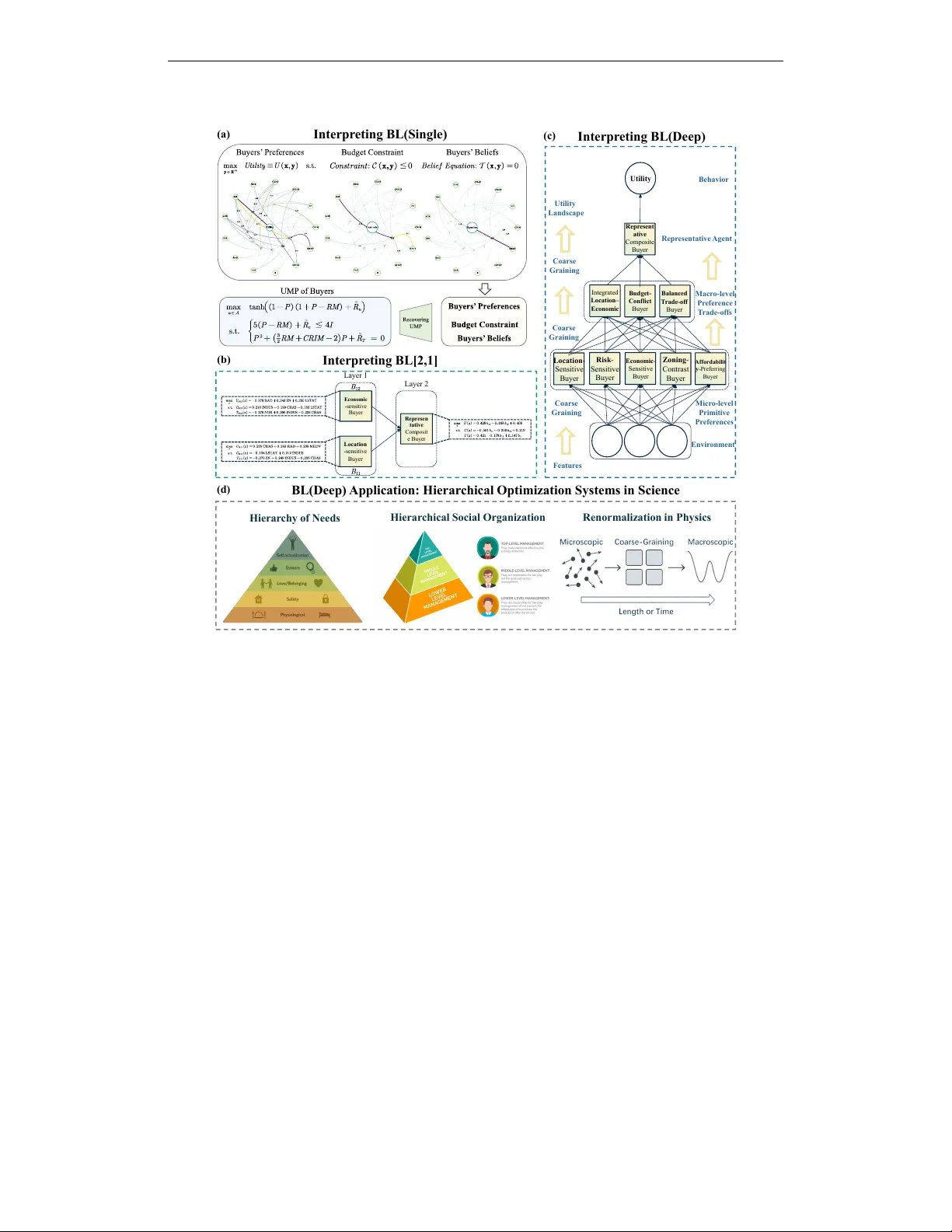
International Conference on Learning Representations (ICLR) 2026 Beha vior Learning (BL): Learning Hierarchical Optimization Structures from Data Zhenyao Ma ∗ Xiamen Univ ersity Y ue Liang Univ ersity of T ¨ ubingen Dongxu Li Xi’an Jiaotong Univ ersity A B S T R AC T Inspired by behavioral science, we propose Behavior Learning (BL), a novel general-purpose machine learning framew ork that learns interpretable and iden- tiﬁable optimization structures from data, ranging from single optimization prob- lems to hierarchical compositions. It uniﬁes predictive performance, intrinsic in- terpretability , and identiﬁability , with broad applicability to scientiﬁc domains in volving optimization. BL parameterizes a compositional utility function built from intrinsically interpretable modular blocks, which induces a data distrib ution for prediction and generation. Each block represents and can be written in sym- bolic form as a utility maximization problem (UMP), a foundational paradigm in behavioral science and a uni versal framew ork of optimization. BL supports archi- tectures ranging from a single UMP to hierarchical compositions, the latter mod- eling hierarchical optimization structures. Its smooth and monotone variant (IBL) guarantees identiﬁability . Theoretically , we establish the uni versal approximation property of BL, and analyze the M-estimation properties of IBL. Empirically , BL demonstrates strong predictiv e performance, intrinsic interpretability and scala- bility to high-dimensional data. Code: MoonYLiang/Behavior-Learning on GitHub; install via pip install blnetwork . Utility Maximization Pr oblem (UMP) Envir onment Behavior Human Behavior Behavior Learning (c) (b) (a) (d) CompU Learning Schem e Data Learnable Learnable Learnable Each Block Learnable UMP BL (Single) Single UMP UMP Composition                                   BL (Deep) BL (S hallow)                                                                     Symbolic Form of Pr ediction Generation Intrinsic Interpr etability V isualization 2 3 4 Interpr etability & Inf er ence Figure 1: Beha vior Learning (BL). (a) Human behavior modeled as a UMP . (b) Learning scheme of BL, where CompU denotes the compositional utility function. (c) BL of fers intrinsic interpretability (via symbolic form as a hierarchical optimization structure), identiﬁability , and inference capability . (d) Three architectural variants of BL, from single UMP to deep compositions. ∗ Correspondence to: zhenyaoma@stu.xmu.edu.cn; Code contact: yue.liang@student.uni-tuebingen.de 1 International Conference on Learning Representations (ICLR) 2026 1 I N T RO D U C T I O N Scientiﬁc research often grapples with phenomena that resist precise formalization ( Anderson , 1972 ; Mitchell , 2009 ), including human and social domains ( Simon , 1955 ; Arthur , 2009 ). Such phenom- ena are dif ﬁcult to predict and e ven harder to falsify through theory alone. Interpretable machine learning (Interpretable ML) ( Molnar , 2020 ), with its po werful approximation capabilities and b uilt- in transparency , of fers a promising alternati ve for modeling such phenomena. Y et a long-standing tension remains unresolved: model predictiv e performance and intrinsic interpretability often trade off—a challenge commonly known as the performance–interpr etability trade-off ( Arrieta et al. , 2020 ). High-performing models such as deep neural networks ( LeCun et al. , 2015 ) typically lack transparency , while intrinsically interpretable models struggle to capture complex nonlinear patterns. Some efforts have been made to mitigate the performance–interpretability trade-off. For exam- ple, Hastie ( 2017 ); Alvarez Melis & Jaakkola ( 2018 ); Angelino et al. ( 2018 ); Nori et al. ( 2019 ); K oh et al. ( 2020 ); Agarwal et al. ( 2021 ); Kraus et al. ( 2024 ); Liu et al. ( 2024b ); Plonsky et al. ( 2025 ) demonstrate varied strengths. Howe ver , two fundamental limitations remain, restricting their scientiﬁc applicability . (i) Insufﬁcient alignment with scientiﬁc theories . Most approaches focus on extending existing machine learning methods to achie ve interpretability , rather than de- veloping a scientiﬁcally grounded frame work (e.g., based on optimization problems or dif ferential equations). This often hinders alignment with scientiﬁc theories and limits the ability to extract scientiﬁc kno wledge from learned models ( Roscher et al. , 2020 ; Bereska & Ga vves , 2024 ; Longo et al. , 2024 ). (ii) Non-uniqueness of interpr etations . Most models are non-identiﬁable —their in- terpretations are not uniquely determined by observ able predictions in a mathematical sense ( Ran & Hu , 2017 ; M ´ eloux et al. , 2025 ). As a result, such models cannot support reliable estimation of ground-truth parameters ( Newe y & McFadden , 1994 ; V an der V aart , 2000 ), and may ev en lack Pop- perian falsiﬁability ( Popper , 2005 ), ultimately limiting their scientiﬁc credibility . These limitations naturally raise a key question: can we design an interpretable ML framework that mitigates the performance–interpretability trade-off while being scientiﬁcally grounded and identiﬁable? Inspired by behavioral science, we propose Behavior Learning (BL) : a general-purpose machine learning framework that learns interpr etable and identiﬁable (hierar chical) optimization structures fr om data . It uniﬁes high predictive performance, intrinsic interpretability , and identiﬁability , with broad applicability to scientiﬁc domains in volving optimization. As illustrated in Figure 1 , BL builds on one of the most fundamental paradigms in behavioral science—utility maximization—which posits that human behavior arises from solving a utility maximization pr oblem (UMP) ( Samuelson , 1948 ; Debreu , 1959 ; Mas-Colell et al. , 1995 ). Motiv ated by this paradigm, BL learns interpretable optimization structures from data. It models responses ( y ) as drawn from a probability distribution induced by a UMP or a composition of multiple interacting UMPs. This distribution is parameterized by a compositional utility function BL( x , y ) , constructed from intrinsically interpretable modular blocks B ( x , y ) . Each block is a learnable penalty-based formulation that represents an optimization problem (UMP), which can be written in symbolic form and offers transparency comparable to linear regression. BL admits hierar chical structur e , mainly in three architectural variants: BL(Single), deﬁned by a single block; BL(Shallo w), a moderately layered composition of blocks; and BL(Deep), a deep hier - archical composition of multiple blocks. The latter two model, and can be symbolically interpreted as, hierarchical optimization structures . All variants are trained end-to-end to induce a condi- tional Gibbs distribution for prediction and generation. By reﬁning the penalty functions in each block into smooth and monotone forms, we dev elop Identiﬁable BL (IBL), the identiﬁable variant of BL. Under mild conditions, IBL guarantees unique intrinsic interpretability . This property ensures the scientiﬁc credibility of its explanations and further supports recovery of the ground-truth model under appropriate conditions. While motiv ated by beha vioral science, BL is not domain-speciﬁc . It applies broadly to any scientiﬁc domain where observed outcomes arise as solutions to optimization problems—such as macroeco- nomics ( Ramsey , 1928 ; Ljungqvist & Sar gent , 2018 ), statistical physics ( Gibbs , 1902 ; Landau & Lifshitz , 2013 ), or evolutionary biology ( Wright et al. , 1932 ; Fisher , 1999 ). This generality is sup- ported by a key theoretical insight (Theorem 2.2 ): any optimization problem can be equiv alently written as a UMP . This makes BL a general-purpose modeling frame work for data-driven inv erse optimization ( Ahuja & Orlin , 2001 ) across div erse scientiﬁc disciplines. 2 International Conference on Learning Representations (ICLR) 2026 W e study BL both theoretically and empirically . Theoretically , we show that both BL and IBL ad- mit uni versal approximation under mild assumptions (Section 2.2 ). For IBL, we further establish its M-estimation properties (Section 2.3 ), including identiﬁability , consistency , universal consistency , asymptotic normality , and asymptotic ef ﬁciency . Empirically , we ev aluate BL across four tasks. Standard prediction tasks (Section 3.1 ) demonstrate its strong predictiv e performance. A qualitativ e case study (Section 3.2 ) illustrates its intrinsic interpretability . Prediction on high-dimensional in- puts (Section 3.3 ) further demonstrates its scalability to high-dimensional data. Further discussion and related work are pro vided in Section 5 and Section 6 , respectiv ely . W e also provide guidance on how to scientiﬁcally e xplain BL(Deep) and architectural details in Section 4 and Section A , respec- tiv ely . Overall, our key contrib utions are threefold. (i) W e propose Behavior Learning (BL), a novel general-purpose machine learning framework inspired by behavioral science, which uniﬁes high predictiv e performance, intrinsic interpretability , identiﬁability , and scalability . (ii) For scientiﬁc re- search, BL offers a scientiﬁcally grounded, interpretable, and identiﬁable machine learning approach for modeling complex phenomena that defy precise formalization. BL applies broadly to scientiﬁc disciplines in volving optimization. (iii) At the paradigm lev el, BL learns from data the optimization structure of either a single optimization problem or a hierarchical composition of problems through distributional modeling, contrib uting a new methodology to data-driv en inv erse optimization. 2 B E H A V I O R L E A R N I N G ( B L ) 2 . 1 U T I L I T Y M A X I M I Z A T I O N P RO B L E M ( U M P ) The modeling of human behavior , particularly in beha vioral science and decision theory , often be- gins with the assumption t hat observed outcomes arise from a latent optimization process. A canon- ical formulation of this idea is the Utility Maximization Problem (UMP) ( Mas-Colell et al. , 1995 ), in which an agent selects actions y ∈ Y in response to contextual features x ∈ X by solving: max y ∈Y U ( x , y ) s.t. C ( x , y ) ≤ 0 , T ( x , y ) = 0 (1) Here, U ( · ) denotes a subjecti ve utility function encoding the agent’ s internal preferences or goals. The inequality constraint C ( · ) captures resource constraints, while the equality constraint T ( · ) en- codes either endogenous belief consistency or e xogenous conservation la ws. The UMP can be recast as a cost–beneﬁt frame work, where the agent trades off utility gains against constraint violations. Formally , under mild regularity conditions, it admits an unconstrained penalty reformulation at the lev el of local optimality ( Han & Mangasarian , 1979 ), as formalized below . Theorem 2.1 (Local Exact Penalty Reformulation for UMP) . Let X ⊂ R d x and Y ⊂ R d y be nonempty compact sets, and let U : X × Y → R , C : X × Y → R m , and T : X × Y → R p be C 1 . Assume that for a given x ∈ X , the Han–Mangasarian constraint qualiﬁcation holds at any strict local maximizer y ⋆ of the UMP . Then ther e exist λ 0 > 0 , λ 1 ∈ R m ++ , and λ 2 ∈ R p ++ such that y ⋆ is a local maximizer of max y ∈Y λ 0 ϕ  U ( x , y )  − λ ⊤ 1 ρ  C ( x , y )  − λ ⊤ 2 ψ  T ( x , y )  . (2) Her e ϕ : R → R is strictly increasing and C 1 , ρ ( z ) := max { z , 0 } , and ψ ( z ) := | z | . The proof is provided in Appendix B.1 . This unconstrained reformulation offers greater tractability for both theoretical analysis and model training. While moti vated by behavioral modeling, the UMP formulation is not domain-speciﬁc. It applies to any setting where observed outcomes are solutions to (explicit or latent) optimization problems. This is because any optimization problem can be equi valently formulated as a UMP . W e state this in the following result, while the formal statement and proof are pro vided in Appendix B.1 . Theorem 2.2 (Univ ersality of UMP) . Any optimization pr oblem of the form max y ∈Y f ( x , y ) or min y ∈Y f ( x , y ) , subject to equality and inequality constraints, is equivalent to a UMP . 3 International Conference on Learning Representations (ICLR) 2026 2 . 2 B L A R C H I T E C T U R E Figure 1 (b–d) illustrates the architecture of BL. W e consider samples ( x , y ) ∼ D , where x ∈ R d denotes conte xtual features and y is the response, represented as ( y disc , y cont ) ∈ Y disc × R m c , cap- turing its hybrid structure. Responses are assumed to be stochastically generated by solving multiple interacting UMPs, each with a penalty-based formulation, which together compose a compositional utility function BL( x , y ) . On this basis, we model the data using a conditional Gibbs distribution ( Gibbs , 1902 ) parameterized by BL Θ ( x , y ) : p τ ( y | x ; Θ) = exp  BL Θ ( x , y ) /τ  Z τ ( x ; Θ) , Z τ ( x ; Θ) = Z Y exp  BL Θ ( x , y ′ ) /τ  d y ′ (3) Here the temperature parameter τ > 0 controls the randomness of the response. As τ → 0 , the distribution in equation 3 con ver ges to a Dirac measure supported on arg max y BL( x , y ) , thereby recov ering the deterministic best response obtained by solving the composed UMPs. Model Structure of BL( x , y ) . T o represent the composition of multiple UMPs, we build BL( x , y ) by composing fundamental modular blocks B ( x , y ) . Each block pro vides a penalty-based formulation of a single UMP , and together the y yield the overall compositional utility function. Motiv ated by Theorem 2.1 , we parameterize B ( x , y ) as B ( x , y ; θ ) := λ ⊤ 0 ϕ  U θ U ( x , y )  − λ ⊤ 1 ρ  C θ C ( x , y )  − λ ⊤ 2 ψ  T θ T ( x , y )  (4) where θ := ( λ 0 , λ 1 , λ 2 , θ U , θ C , θ T ) denotes the complete set of learnable parameters. Following Theorem 2.1 , ϕ is an increasing function; ρ penalizes inequality violations; and ψ captures symmet- ric deviations. Each block can be written as a well-deﬁned UMP . W e then compose BL( x , y ) from multiple B -blocks through hierarchical composition to improv e its representational power for optimization structures, yielding three main architectural variants, as illustrated in Figure 1 (d). 1. BL(Single) applies a single instance of B ( x , y ) as deﬁned in equation 4 , without any additional layers. It can be vie wed as learning a single UMP , and offers maximal interpretability . 2. BL(Shallo w) uses B ( x , y ) as the fundamental modular block to construct a shallow net- work. It introduces one or two intermediate layers of computation. Each layer B ℓ stacks multiple parallel B ℓ,i blocks to produce a vector in R d ℓ , i.e., B ℓ ( x , y ; θ ℓ ) := [ B ℓ, 1 ( x , y ; θ ℓ, 1 ) , . . . , B ℓ,d ℓ ( x , y ; θ ℓ,d ℓ )] ⊤ . The output of B ℓ is directly fed into the next B ℓ +1 , and only the ﬁnal output is passed through a learnable afﬁne transformation. 3. BL(Deep) e xtends the BL(Shallo w) architecture to more than two layers, enabling richer hierar- chical compositions of UMPs while maintaining the same recursi ve structure. As before, only the ﬁnal output is afﬁne transformed. The ov erall structure of BL(Shallow) and BL(Deep) can be expressed in a uniﬁed form, where the shallow case corresponds to L ≤ 2 and the deep case to L > 2 : BL( x , y ) := W L · B L  · · · B 2 ( B 1 ( x , y )) · · ·  (5) Learning Objective. The response y may contain both discrete and continuous components. For discrete responses, we directly apply cross-entropy ( Kullback & Leibler , 1951 ) on y disc . For contin- uous responses, since the compositional utility function is analogous to an energy function ( LeCun et al. , 2006 ), we employ denoising score matching ( V incent , 2011 ) on y cont . The ﬁnal objecti ve combines the two with nonneg ativ e weights γ d , γ c : L ( θ ) = γ d E  − log p τ ( y disc | x )  + γ c E   ∇ ˜ y cont log p τ ( ˜ y cont | x ) + σ − 2 ( ˜ y cont − y cont )   2 (6) Implementation Details. Here, we describe the key implementation choices for the general form of BL, taken as defaults unless otherwise noted. Further details are provided in Appendix A.3 . • Function Instantiation. Following equation 4 , we instantiate the function B ( x , y ) as B ( x , y ) = λ ⊤ 0 tanh  p u ( x , y )  − λ ⊤ 1 ReLU  p c ( x , y )  − λ ⊤ 2   p t ( x , y )   (7) 4 International Conference on Learning Representations (ICLR) 2026 where p u , p c , p t are polynomial feature maps of bounded degree, pro viding interpretable rep- resentations of utility , inequality , and equality terms, respectively . The bounded tanh reﬂects the principle of diminishing marginal utility ( Jevons , 2013 ), a commonly assumed principle in behavioral science, while ReLU and | · | introduce soft penalties for constraint violations. • Polynomial Maps. In BL(Single), the structure of polynomial maps is optional. In BL(Shallow) and BL(Deep), each B -block employs afﬁne transformations as its polynomial maps, with higher-de gree and interaction terms omitted by default for computational ef ﬁciency . • Skip Connections. For deep variants, skip connections can be optionally introduced to improve representational efﬁcienc y . More detailed architectural descriptions for this section are pro vided in Appendix A . Theoretical Guarantees. Under the given architecture, the BL framework has univ ersal approxi- mation power: it can approximate any continuous conditional distribution arbitrarily well, provided that BL has sufﬁcient capacity , as stated below . The proof is gi ven in Appendix B.2 . Theorem 2.3 (Uni versal Approximation of BL) . Let X ⊂ R d and Y ⊂ R m be compact sets, and let p ⋆ ( y | x ) be any continuous conditional density such that p ⋆ ( y | x ) > 0 for all ( x , y ) ∈ X × Y . Then for any τ > 0 and ε > 0 , ther e exists a ﬁnite BL ar chitectur e (with depth and width depending on ε ) and a parameter θ ⋆ such that the Gibbs distrib ution in equation 3 satisﬁes sup x ∈X KL  p ⋆ ( · | x ) ∥ p τ ( · | x ; θ ⋆ )  < ε. (8) Interpr etability . Alongside its expressi ve po wer , BL also e xhibits strong intrinsic interpretability . • Each B -block can be expressed in symbolic form as an optimization problem (UMP): the tanh term deﬁnes the objective, the ReLU term corresponds to an inequality constraint, and the absolute-value term corresponds to an equality constraint. Thus, BL(Single) can be directly expressed as a symbolic UMP , whereas deeper architectures can be interpreted as compositions of UMPs, with each block retaining interpretability . • The polynomial basis ensures a level of transparency comparable to linear regr ession , as both objectives and constraints can be represented as linear combinations of polynomial features. It can further be visualized as a computational graph (Figure 7 ), in which each input’ s inﬂuence on ev ery B -block is traceable through compositional pathways. • BL(Deep) composes B -blocks in a layered manner , forming a hierarchical optimization struc- ture . Interpretation proceeds in a bottom-up fashion, where the relation between any two consec- utiv e layers can be viewed as aggregation or coarse-grained observation. Overall, the interpretiv e pathway is: raw input featur es → micr o-level optimization bloc ks → macr o-level aggr e gation or coarse-grained behavioral constructs → macr o-level optimization systems . Section 4 pro vides a detailed description of this interpretation procedure. • BL also of fers multiple architectural de grees of freedom that pro vide ﬂexibility but simultane- ously af fect the resulting interpretability . In deep variants, skip connections introduce cross- layer dependency structures that are modeled in statistical physics ( Y ang & Schoenholz , 2017 ). Replacing polynomial maps with af ﬁne transformations preserves the underlying optimization semantics but reduces symbolic granularity , yielding a more qualitativ e rather than symbolic interpretation of each block. • BL can be interpreted as a single UMP when the ﬁnal layer contains only one B -block, since all lo wer-layer structures aggregate into a uniﬁed optimization problem. When the ﬁnal layer contains multiple B -blocks, BL corresponds to a linear trade-off among multiple optimization problems. 2 . 3 I D E N T I FI A B L E B E H A V I O R L E A R N I N G ( I B L ) Beyond prediction and interpretability , the BL framework supports a third fundamental goal: the identiﬁcation of gr ound-truth parameters , which in turn endows BL with the capacity for scientiﬁ- cally credible modeling. W e refer to this setting as Identiﬁable Beha vior Lear ning (IBL) . In the 5 International Conference on Learning Representations (ICLR) 2026 L ay er 1 E co no m ic - se nsi t i v e B uy er L ocat i on - se nsi t i v e B uy er R epres en t at i ve C om posi t e B uy er L ay er 2 Hier ar chy of Needs Hier ar chic al So ci al Orga niz at io n Reno rmali z at io n in Phy sic s Lo ca ti o n - Sen s i t i v e Bu y er E c on om ic - S e nsit ive B uy e r R i s k - Sen s i t i v e Bu y er Z o ni ng - Co n t ras t Bu y er A f f orda bi l i t y - Pre f er r i ng B uy er I nteg ra t e d L oc ation – E c on om ic B u d ge t - Conf li c t B uy e r B alan c e d T r ad e - of f B uy e r Re p r e se n t ative C ompos it e B uy e r U ti l i ty M a cr o - l ev el P r efer ence T ra de - o ffs R epr es enta ti v e A g ent M i cr o - l ev el P ri m i ti v e P r efer ences Env i r o nm ent Beha v i o r C o a rs e Gra i ni ng C o a rs e Gra i ni ng C o a rs e Gra i ni ng F ea tur es U ti l i ty La nds ca pe (d ) BL (Deep) Ap pli cat ion: Hi erar chical Opt im iz ati on Syste ms in Sci ence (b ) Inter pr eti ng BL [2,1] (a ) Inter pr eti ng BL (Singl e) (c) Interpr eti ng BL (Deep) Figure 2: (a) V isualization and symbolic form of BL(Single) trained on the Boston Housing dataset, modeling the UMP ( max U s.t. C ≤ 0 , T = 0 ) of a representati ve b uyer in Boston housing (details in Section 3.2 ). T op: computational graphs of the polynomials inside the three penalty functions— tanh (preference), ReLU (budget), and | · | (belief). Each graph is respecti vely centered on tanh − 1 ( U ) , C , and T from left to right, with surrounding nodes representing input features. Directed edges (shown only if coef ﬁcient ≥ 0 . 3 ) indicate ho w each feature contributes to the corre- sponding term. Bottom: approximate symbolic formulation of the trained BL model as a UMP . (b) The BL[2,1] architecture. Layer 1 identiﬁes two k ey micro-lev el preference types: the Economic- sensitive Buyer and the Location-sensitive Buyer . Layer 2 aggreg ates these two components into an effecti ve representativ e buyer . (c) The BL(Deep) [5,3,1] architecture. Layer 1 recov ers ﬁve distinct micro-lev el housing preference types. Layer 2 identiﬁes three macro-le vel trade-off types captur - ing different ways these primitive preferences interact. Layer 3 aggregates them into the ov erall representativ e buyer . T able 10 provides detailed descriptions of each type. BL(Deep) provides a hierarchical e xplanation consistent with the coarse-graining principle ( Kadanoff , 1966 ) in statistical physics, reconstructing the full micro-to-macro optimization hierarchy . In addition, the preference and trade-of f patterns uncov ered by BL(Deep) are well documented in the classical economics liter- ature (see T able 11 ). (d) BL can be applied to a broad class of hierarchical optimization structures in science, including hierarchical need structures, hierarchical social–org anizational structures, and renormalization-style coarse-grained structures in physics. IBL setting, we deﬁne the modular block as B id ( x , y ; θ ) := λ ⊤ 0 ϕ id  U θ U ( x , y )  − λ ⊤ 1 ρ id  C θ C ( x , y )  − λ ⊤ 2 ψ id  T θ T ( x , y )  (9) Unlike BL, which uses general nonlinearities, the IBL architecture imposes stricter structural con- straints: ϕ id and ρ id are strictly increasing, while ψ id is symmetric and strictly increasing in | · | . In addition, all three functions are C 1 . These properties ensure that each UMP block stays responsi ve 6 International Conference on Learning Representations (ICLR) 2026 and adjusts smoothly to objectiv es and constraints. In practice, we instantiate equation 9 as B id ( x , y ) = λ ⊤ 0 tanh  p u ( x , y )  − λ ⊤ 1 softplus  p c ( x , y )  − λ ⊤ 2  p t ( x , y )  ⊙ 2 (10) where ( · ) ⊙ 2 denotes elementwise square. W e design IBL in three architectural forms. Similar to BL, the IBL(Single) directly uses B id ( x , y ) as the compositional utility function. The IBL(Shallow) and IBL(Deep) variants are deﬁned recursiv ely as IBL( x , y ) := W ◦ L · B id L  · · · B id 2  B id 1 ( x , y )  · · ·  , L ≥ 1 (11) where B id ℓ stacks multiple parallel blocks B id ℓ,i ( x , y ) , and W ◦ L is a learnable afﬁne transformation without bias. All other design choices follo w the BL setting. Theoretical F oundation. IBL admits fav orable properties for ground-truth identiﬁcation. W e be- gin by establishing identiﬁability , which is fundamental for statistical inference. W e ﬁrst state our key assumption (see Assumption B.1 for details). Assumption 2.1. Let ¯ Ψ denote the quotient space of atomic parameters. W e assume that the map ¯ Ψ → R X ×Y , ¯ ψ 7→ g ¯ ψ , is injective , and that any ﬁnite set of distinct atoms is linearly indepen- dent . W e further r estrict attention to minimal representations with no duplicate atoms and a ﬁxed canonical or dering. Theorem 2.4 (Identiﬁability of IBL) . Under Assumption B.1 , the arc hitectur es IBL(Single), IBL(Shallow), and IBL(Deep) ar e identiﬁable in the parameter quotient space ¯ Θ . Theorem 2.5 (Loss Identiﬁability of IBL) . The IBL model is par ameterized by θ ∈ Θ . Suppose Θ is compact. Then under Assumption B.1 , the population loss L deﬁned in equation 6 satisﬁes: • If γ c > 0 , it admits a unique minimizer in the quotient space ¯ Θ ; • If γ c = 0 , it admits a unique minimizer in the scale-in variant quotient space e Θ . Theorems 2.4 and 2.5 together establish the identiﬁability of IBL. Theorem 2.4 shows that if two IBL models of the same structure induce the same compositional utility , then their parameters coincide up to an equiv alence class. Theorem 2.5 further extends this result to loss-based identiﬁability . These results jointly imply that IBL admits a unique parameter estimate up to an equi valence class, and thus yields intrinsic interpretability that is unique up to the same class. Building on identiﬁability , Theorem 2.6 establishes the statistical consistency of IBL: under com- pactness of the parameter space, the learned parameters conv erge in probability to a minimizer of the population loss as the sample size n → ∞ . If the model is correctly speciﬁed, the estimator further con verges to the ground-truth parameter , reco vering the true underlying model , thereby endowing IBL with the potential to recov er the ground-truth model. Theorem 2.6 (Consistency of IBL) . Let Ξ denote the r elevant parameter quotient space: Ξ = ¯ Θ if γ c > 0 , and Ξ = e Θ if γ c = 0 . Let ˆ θ n ∈ arg min θ ∈ Θ M n ( θ ) denote the empirical minimizer , and let θ • ∈ arg min θ ∈ Θ M ( θ ) denote the population minimizer . Then under the conditions of Theor em B.5 , ˆ θ n p − → θ • in Ξ , M ( ˆ θ n ) p − → M ( θ • ) . Mor eover , if the model is correctly speciﬁed (i.e., the data distribution is realized by some θ ⋆ ∈ Θ ), then θ • = θ ⋆ in Ξ , and thus ˆ θ n p − → θ ⋆ . Correct speciﬁcation is a strong and often unrealistic assumption. Fortunately , the IBL frame- work—like BL—also enjoys a univ ersal appr oximation guarantee (Theorem B.6 ). Building on this result, we further establish the universal consistency of IBL: even under misspeciﬁcation, IBL is capable of r ecovering the gr ound-truth model with sufﬁciently lar ge sample sizes. Theorem 2.7 (Uni versal Consistenc y of IBL) . Under the conditions of Theor em B.7 , for any admis- sible data-gener ating distrib ution p † satisfying the re gularity assumptions of Theorem B.6 , the IBL posterior sequence { p ˆ θ n } satisﬁes sup x ∈X KL  p † ( · | x ) ∥ p ˆ θ n ( · | x )  p − → 0 , i.e., the learned conditional distrib utions { p ˆ θ n } con ver ge in KL to p † uniformly over x . 7 International Conference on Learning Representations (ICLR) 2026 Speciﬁcally , this result implies that, e ven under model misspeciﬁcation, the learned predictive dis- tribution p ˆ θ n , parameterized by the IBL model, con verges uniformly in KL to the true conditional distribution p † , provided that the capacity of the IBL architecture gro ws with the sample size n . W e also establish the asymptotic normality of IBL estimators (Theorem B.9 ), showing that the parameter estimates conv erge in distribution to a normal law as the sample size increases. Further- more, under additional regularity conditions, the asymptotic variance attains the efﬁcient informa- tion bound (Theorem B.10 ), demonstrating the statistical optimality of IBL. Formal statements and proofs of all theorems in this part are deferred to Appendix B.3 . 3 E X P E R I M E N T S In this section, we conduct four groups of experiments to systematically ev aluate the capabilities of BL. Due to space constraints, details are provided in Appendix C . 3 . 1 S TA N D A R D P R E D I C T I O N T A S K S P erform anc e S core s O n 10 dat as et s × 8 se eds AUC boxpl ot P erform anc e Ranks O n 10 dat as et s × 8 se eds Sort ed by m ea n F1 - Mac ro r ank P erform anc e S core s O n 10 dat as et s × 8 se eds F1 - Mac ro boxpl ot Figure 3: Predictive performance of BL and baselines. Left/Middle: relative A UC and F1-Macro gains ov er DT , sorted by mean (excluding BL). Right: mean F1-Macro ranks ( ↓ better). BL achie ves ﬁrst-tier performance in both metrics. Its v ariants rank second and third in mean F1-Macro rank, with BL(Shallow) sho wing no statistically signiﬁcant difference from state-of-the-art models. Is BL accurate enough for standar d pr ediction tasks? In this part, we ev aluate the predictive performance of BL on 10 datasets (T able 4 ), cov ering di verse sample sizes, feature dimensions, and scientiﬁc domains. F or fair comparison, we consider two BL variants—BL(Single) and BL(Shallow)—and compare them against 10 baseline models (T able 5 ) drawn from ﬁv e method- ological families: neural networks, tree-based models, gradient boosting methods, Bayesian meth- ods, and linear regressors. All methods share a uniﬁed preprocessing and tuning pipeline. Predicti ve Perf ormance. Figure 3 shows that BL attains ﬁrst-tier predicti ve performance o verall, achieving the best results among intrinsically interpretable models. Notably , BL(Shallow) surpasses MLP , highlighting that BL delivers interpretability without sacriﬁcing performance. 8 International Conference on Learning Representations (ICLR) 2026 3 . 2 I N T E R P R E T I N G B L : A C A S E S T U D Y How can BL be interpr eted in practice? This part presents a case study using the Boston Housing dataset, where we train a supervised BL(Single) model with a degree-2 polynomial basis, a BL[2,1] model (i.e., a tw o-layer BL with two B-blocks in the ﬁrst layer and one in the second layer), and a BL(Deep) model with a [5,3,1] architecture to predict median home values. W e illustrate how the internal structure of BL can be interpreted as explicit optimization problems and their hier- archical versions, accompanied by complementary visualizations. Further details are provided in Appendix C.3 and C.5 . Symbolic F orm of BL(Single) as a UMP . As shown in Figure 2 , the trained BL(Single) model can be interpreted as the UMP of a repr esentative buyer in the Boston Housing market, comprising a single objecti ve, inequality , and equality term. Each term is represented by an estimated quadratic polynomial. F or parsimony , we extract approximate symbolic expressions by retaining only the monomials with the largest (2–5) absolute coefﬁcients, while collecting the remaining terms (in- cluding constants) into a residual term ˜ R . F or example, the utility term can be written as: p u = − 0 . 56 · P 2 − 0 . 6 · RM + 0 . 57 · RM · P + ˜ R u ≈ (1 − P )(1 + P − RM) + ˜ R u W e similarly simplify the budget and belief terms to recover an approximate UMP for the buyer . The full symbolic form is illustrated at the bottom of Figure 2 . Interpr eting BL(Single) via Model Visualization. V isualizations of each term’ s polynomial re- veal ho w features constitute the UMP . Three insights emerge from the visualizations in Figure 2 . (i) Median housing price (MED V) and aver age number of r ooms (RM) are dominant across all terms—MED V negativ ely affects utility in a near -quadratic form, while RM modulates its marginal effect. (ii) Pr oportion of lower-income residents (LST AT) features prominently in the budget con- straint, reﬂecting implicit resource limitations. (iii) Crime rate (CRIM) appears only in the belief term, suggesting that b uyers treat it as inﬂuencing others’ behavior rather than their own preferences. Figure 4: Interpreting deeper BL architectures as hierarchical structures of interacting agents. Each block B represents an interpretable agent solving its o wn UMP , while a layer corresponds to a set of heterogeneous agents operating in parallel. The next layer then aggregates and reallocates the neg- ativ e energies from the pre vious layer , thereby performing higher-le vel coordination across agents. This layered org anization provides a natural compositional interpretation of deep BL: bottom-layer modules encode local objectiv es, while upper layers synthesize these into collective outcomes. Anal- ogous structures arise in biological and social systems—for example, in ant colonies, indi vidual ants (ﬁrst-layer agents) follow simple local rules, yet their collecti ve behavior is coordinated through higher-le vel interactions (second-layer aggregation), yielding globally efﬁcient resource allocation and task division. 9 International Conference on Learning Representations (ICLR) 2026 Interpr eting BL(Deep). (1) Figure 2 (b) illustrates the optimization problems learned by the BL[2,1] model. Layer 1 identiﬁes two micro-level preference types: an Economic-sensitive Buyer , whose utility and constraint terms load primarily on ZN (Large-lot residential share) and LST A T (Proportion of lower -income residents); and a Location-sensitive Buyer , driven mainly by CHAS (Charles Ri ver indicator) and RAD (Highway accessibility). Layer 2 aggre gates these basic pref- erences, yielding an effecti ve “representativ e buyer” that integrates the two preference types. (2) Figure 2 (c) presents the internal structure of the BL[5,3,1] model. In Layer 1, BL recov ers ﬁv e distinct micr o-level pr eference types characterizing heterogeneous patterns in the housing market. Layer 2 identiﬁes three macro-le vel representative agents, each capturing a dif ferent macr o-level trade-of f among the basic preferences. Layer 3 then aggre gates these components into a single high-lev el mechanism, yielding the ov erall representati ve buyer . T able 10 pro vides detailed descrip- tions of each type. (3) Beyond interpretability , we ﬁnd that each preference pattern and trade-of f recov ered by BL(Deep) aligns with established ﬁndings in the economics literature (see T able 11 ). This indicates that BL successfully reconstructs underlying scientiﬁc knowledge. 3 . 3 P R E D I C T I O N O N H I G H - D I M E N S I O N A L I N P U T S Is BL scalable to high-dimensional inputs? W e e valuate BL against the ener gy-based MLP (E- MLP) baseline across network depths d ∈ { 1 , 2 , 3 } , with all models implemented without skip connections. Experiments are conducted on four datasets spanning both image and text domains, and are ev aluated using six metrics : in-distribution accuracy , calibration metrics (ECE and NLL), and OOD robustness metrics (A UROC, A UPR, and FPR@95). For OOD ev aluation, we adopt symmetric ID ↔ OOD splits, using MNIST ( LeCun et al. , 2002 ) and Fashion-MNIST ( Xiao et al. , 2017 ) as one pair, and AG Ne ws and Y elp Polarity ( Zhang et al. , 2015 ) as another . E-MLP and BL are controlled to hav e comparable parameters. Scalability on High-Dimensional Inputs. Figure 5 and T able 1 present results for BL and E-MLP across network depths. On image datasets, the tw o models exhibit comparable in-distribution ac- curacy , while BL generally achie ves stronger out-of-distribution detection performance on Fashion- MNIST at similar accuracy le vels. On text datasets, BL consistently improves ID accuracy ov er E-MLP across depths. Ho wev er , OOD detection behavior varies by dataset: BL outperforms E- MLP on Y elp, whereas E-MLP shows better OOD discrimination on A G News. BL also achie ves better calibration metrics (ECE and NLL; T able 2 ). Downward Shift of the Par eto Frontier . T able 13 reports the parameter counts of BL and E-MLP across four tasks, and T ables 3 summarize their runtimes. The two models hav e highly comparable parameter sizes. Across datasets, BL exhibits slightly higher training time than E-MLP . Combining these results with their comparable predictiv e performance and the intrinsic interpretability of BL, in contrast with the black-box E-MLP , indicates that BL achieves a downwar d shift of the Pareto frontier . 3 . 4 C O N S T R A I N T E N F O R C E M E N T T E S T : H I G H - D I M E N S I O NA L E N E R G Y C O N S E RV AT I O N T o e valuate whether the learnable penalty terms in BL are capable of enforcing near -hard constraints under ﬁnite temperature, we isolate the penalty mechanism and test it on a high-dimensional energy- conservation constraint. This diagnostic experiment remov es the utility term and focuses solely on the penalty term, pro viding a characterization of how the penalty term controls constraint violations as a function of temperature τ and penalty scale λ . Experiment setup. W e sample x ∈ R 64 i.i.d. from a standard Gaussian x ∼ N (0 , I 64 ) and deﬁne a pure penalty compositional utility T ( x, y ) = ∥ y ∥ 2 − ∥ x ∥ 2 , BL ( x, y ) = − λ T ( x, y ) 2 , which plays the role of an energy-conserv ation residual and its quadratic penalty . W e target the Gibbs distrib ution p ( y | x ) ∝ exp  BL ( x, y ) /τ  10 International Conference on Learning Representations (ICLR) 2026 Figure 5: Comparison of BL and E- MLP on image and text datasets; d de- notes model depth. T able 1: ID accurac y and OOD A UROC (%) on image and text datasets. BL and E-MLP are ev aluated at depths 1–3 with matched parameter counts, both without skip connec- tions. T op-two per column are blue and red . Image Datasets Model MNIST Fashion-MNIST Accuracy OOD A UROC Accurac y OOD A UR OC E-MLP (depth=1) 98.15 ± 0.07 88.72 ± 1.36 88.79 ± 0.29 90.57 ± 1.39 BL (depth=1) 97.97 ± 0.18 91.17 ± 2.68 89.26 ± 0.22 91.89 ± 0.71 E-MLP (depth=2) 98.11 ± 0.08 90.32 ± 1.74 88.88 ± 0.26 84.61 ± 2.56 BL (depth=2) 98.05 ± 0.12 90.57 ± 2.49 88.96 ± 0.39 89.87 ± 2.48 E-MLP (depth=3) 98.14 ± 0.11 87.76 ± 2.55 89.33 ± 0.25 83.13 ± 1.90 BL (depth=3) 97.93 ± 0.27 92.92 ± 1.69 88.79 ± 0.25 89.24 ± 4.18 T ext Datasets Model A G News Y elp Accuracy OOD A UROC Accurac y OOD A UR OC E-MLP (depth=1) 88.74 ± 0.26 59.24 ± 0.21 91.16 ± 0.02 57.60 ± 0.31 BL (depth=1) 89.52 ± 0.16 66.18 ± 0.20 91.56 ± 0.04 57.06 ± 0.10 E-MLP (depth=2) 89.29 ± 0.20 62.48 ± 0.76 91.32 ± 0.09 57.47 ± 0.21 BL (depth=2) 89.22 ± 0.20 63.68 ± 0.46 91.39 ± 0.06 57.31 ± 0.27 E-MLP (depth=3) 89.37 ± 0.21 66.82 ± 1.01 91.23 ± 0.07 57.36 ± 0.27 BL (depth=3) 88.80 ± 0.18 64.44 ± 0.52 91.13 ± 0.09 57.16 ± 0.48 T able 2: ECE and NLL on image and text datasets. BL and E-MLP are e valuated at depths 1–3 with matched parameter counts. T op-two per column are blue and red . Model MNIST Fashion-MNIST ECE NLL ECE NLL E-MLP (depth=1) 0.02 ± 0.00 0.20 ± 0.02 0.08 ± 0.00 0.74 ± 0.01 BL (depth=1) 0.02 ± 0.00 0.26 ± 0.01 0.05 ± 0.00 0.36 ± 0.01 E-MLP (depth=2) 0.02 ± 0.00 0.23 ± 0.02 0.09 ± 0.00 0.89 ± 0.03 BL (depth=2) 0.02 ± 0.00 0.16 ± 0.01 0.07 ± 0.00 0.44 ± 0.01 E-MLP (depth=3) 0.02 ± 0.00 0.16 ± 0.02 0.09 ± 0.00 0.85 ± 0.04 BL (depth=3) 0.02 ± 0.00 0.13 ± 0.02 0.07 ± 0.00 0.49 ± 0.02 Model A G News Y elp ECE NLL ECE NLL E-MLP (depth=1) 0.02 ± 0.00 0.40 ± 0.01 0.01 ± 0.00 0.24 ± 0.00 BL (depth=1) 0.02 ± 0.00 0.31 ± 0.01 0.00 ± 0.00 0.20 ± 0.00 E-MLP (depth=2) 0.02 ± 0.00 0.42 ± 0.01 0.00 ± 0.00 0.25 ± 0.00 BL (depth=2) 0.06 ± 0.01 0.43 ± 0.03 0.02 ± 0.00 0.23 ± 0.01 E-MLP (depth=3) 0.01 ± 0.00 0.41 ± 0.02 0.00 ± 0.00 0.25 ± 0.01 BL (depth=3) 0.05 ± 0.01 0.39 ± 0.02 0.02 ± 0.00 0.22 ± 0.00 T able 3: T raining time (seconds) of BL vs. E-MLP on high-dimensional datasets (mean ± std). Model MNIST FashionMNIST A G News Y elp E-MLP (depth=1) 100.59 ± 0.29 73.57 ± 1.20 14.69 ± 0.40 179.37 ± 0.73 BL (depth=1) 110.63 ± 3.34 96.52 ± 2.90 17.20 ± 0.06 181.07 ± 1.80 E-MLP (depth=2) 102.64 ± 0.26 78.25 ± 0.28 15.76 ± 0.06 179.22 ± 0.66 BL (depth=2) 122.85 ± 3.95 114.43 ± 3.72 21.78 ± 0.08 180.38 ± 1.44 E-MLP (depth=3) 104.52 ± 0.30 85.57 ± 1.19 16.95 ± 0.05 178.99 ± 1.42 BL (depth=3) 140.17 ± 4.42 130.03 ± 4.96 26.29 ± 0.24 180.36 ± 0.91 11 International Conference on Learning Representations (ICLR) 2026 using ov erdamped Langevin dynamics with step size η = 10 − 4 : y k +1 = y k + η ∇ y B L ( x, y k ) /τ + p 2 η τ ξ k , ξ k ∼ N (0 , I 64 ) . For each pair ( λ, τ ) we run 512 parallel chains, each for 1500 Langevin steps (500 b urn-in). W e sweep over temperatures τ ∈ { 2 . 0 , 1 . 0 , 0 . 5 , 0 . 25 , 0 . 1 , 0 . 05 , 0 . 02 , 0 . 01 , 0 . 005 } at a ﬁxed penalty λ = 25 , and ov er penalty weights λ ∈ { 0 , 1 , 3 , 10 , 30 , 100 , 200 , 500 } at a ﬁx ed temperature τ = 0 . 05 . For each conﬁguration we record the residual magnitude | T ( x, y ) | from the ﬁnal state of every chain. W e then report three summary statistics: (i) the mean violation E [ | T ( x, y ) | ] , (ii) the 95 th percentile of | T ( x, y ) | , and (iii) the empirical probability of near-feasible samples. W e declare a sample to satisfy the constraint approximately if | T ( x, y ) | ≤ ε tol with ε tol = 10 − 1 , and estimate P ( | T ( x, y ) | ≤ ε tol ) across chains. This tolerance scale is chosen to be small relativ e to the typical unconstrained residuals, so that the near-feasible regime corresponds to a practically tight energy-conserv ation constraint. Figure 6: Constraint enforcement test of the BL penalty block on an energy-conserv ation constraint. The ﬁgure reports violation statistics | T ( x, y ) | when varying the temperature τ (left side of panel) and the penalty weight λ (right side of panel). Constraint enforcement. Figure 6 sho ws that BL achiev es near-hard constraint enforcement un- der ﬁnite temperature and penalty scaling. V iolations decrease substantially as τ decreases or λ increases. At around λ = 25 and τ = 0 . 01 , the 64-dimensional ener gy-conserv ation constraint is enforced within 10 − 2 error . Curv es remain mostly smooth and monotone in 64 dimensions, indicat- ing stable Langevin sampling and ef fective penalty enforcement. 4 S C I E N T I FI C E X P L A N A T I O N O F B L ( D E E P ) BL(Deep) provides a form of interpretability that is consistent with hierarchical optimization struc- tures. In BL, each layer performs a coarse-graining of the optimization structure implemented by the layer below . An intuitive analogy is a corporate organizational hierarchy: lower-layer managers 12 International Conference on Learning Representations (ICLR) 2026 solve their own local optimization problems, while higher-layer managers aggregate and coordi- nate the outcomes of many such lower -layer problems to achieve broader or ganizational objectiv es. BL(Deep) follows the same principle—higher layers summarize, reor ganize, and coordinate the so- lutions formed at lower layers. This perspecti ve aligns with man y scientiﬁc domains characterized by multi-le vel complexity , in- cluding (i) the formation of representativ e behavioral agents in behavioral sciences, and (ii) renor - malization in statistical physics, where ﬁne-scale interactions are compressed into effecti ve coarse- scale potentials. W e describe the explanation procedure below . T o build intuition, let us ﬁrst consider a generic hier- archical optimization structure—this may refer to a multi-layer or ganizational structure composed of individual agents, or a multi-scale ph ysical system composed of interacting particles. Step 1: Bottom-lay er interpretation. Each bottom-layer block is an optimization problem that directly receiv es inputs from the environ- ment. These blocks correspond to micr o-level behavioral mechanisms , such as the decision rules of indi vidual agents performing en vironment-facing tasks in an organization, or the motion laws gov erning a single particle in statistical physics. Examining these bottom-layer blocks rev eals the fundamental optimization principles followed by all units that directly interact with the en vironment. Step 2: Lay er -wise coarse-graining and micro-to-macr o aggregation. Blocks in the next layer aggregate the outputs of lo wer-layer optimization problems through a new optimization step, producing a coarse-gr ained behavioral summary . Each higher-le vel block repre- sents the effecti ve optimization system that emerges from the interactions among many lower -lev el units, thereby capturing macro-lev el regularities distilled from micro-lev el mechanisms. This micro-to-macro transition is consistent with many well-established scientiﬁc principles, includ- ing: • (i) Aggregation and coordination : in hierarchical or ganizations, the outputs of lo wer-le vel agents are aggregated, reallocated, and coordinated by higher-le vel agents to achieve improved organizational objecti ves. • (ii) Coarse-grained observation : in hierarchical behavioral systems, indi vidual agents are grouped into categories that share characteristic optimization patterns; in statistical physics, many particles collectively form systems whose coarse-grained behavior is governed by effecti ve potentials induced by microscopic interactions. Step 3: Bottom-up r econstruction. A global explanation is obtained by tracing the hierarchy upward, follo wing the model’ s micro- to-macro abstraction path: ra w input features → micro-le vel optimization blocks → macro-level aggregation and coordination or coarse-grained behavioral constructs → macro-level optimization system. At each layer , we inspect the characteristics of each block and its associated optimization objectiv e, as well as how these optimization problems e volv e across layers. This re veals how each higher layer aggregates, coordinates, or coarse-grains the outputs of the layer belo w . T ogether , these observ ations yield a compact multi-scale interpretation in which BL is understood as a hierarchical optimization structure. 5 D I S C U S S I O N In what follo ws, we discuss the limitations and futur e directions of Behavior Learning from the perspectiv es of theoretical foundations, architecture, and applications. Scalability of theoretical assumptions. The identiﬁability-related statistical theorems constitute the core theoretical pillars of IBL, ensuring uniqueness of the interpretability and supporting its scientiﬁc credibility . Although these results hold under mild conditions, their behavior in large-scale, highly ov er-parameterized architectures remains less well understood. This highlights the need for 13 International Conference on Learning Representations (ICLR) 2026 systematic inv estigations into the robustness, potential failure modes, and empirical boundaries of these guarantees when applied to modern large-scale learning systems. Choice of basis functions. Polynomial basis functions enhance expressi vity while preserving symbolic interpretability in BL (Single). Howe ver , high-order polynomials may introduce optimiza- tion instability , exacerbate sensitivity to initialization and normalization, and complicate training dynamics. Future work may e xplore alternati ve basis families—such as trigonometric, spline-based, or neural basis functions—and develop conditioning or normalization strategies that improv e nu- merical stability without sacriﬁcing interpretability . Interpr etable generativ e modeling . BL integrates several training techniques from ener gy-based models while retaining intrinsic interpretability , enabling interpretable generative modeling for vi- sion (e.g., image or video generation) and language (e.g., lar ge language models). Extending BL to explicitly generativ e architectures in which outputs correspond directly to human-understandable and scientiﬁcally meaningful blocks represents a compelling direction. Such extensions could yield generativ e systems with greater transparency , controllability , and scientiﬁc credibility compared to traditional black-box models. Hybrid architectures for partial interpretability . A promising direction for future work is to dev elop hybrid architectures that inte grate BL with black-box models in a principled way to achie ve partial interpretability . Three a venues are particularly worth exploring: (i) Feature-lev el integra- tion. Black-box neural networks can serve as high-capacity feature extractors, while BL operates on the resulting learned representations to impose structured, optimization-based semantics. (ii) Decision-critical inte gration. BL blocks may be inserted speciﬁcally at high-risk or decision-critical components of the model, substantially reducing the interpretability and reliability risks associated with purely black-box architectures. (iii) Mechanism-lev el integration. Because BL provides an optimization-driv en inductive bias aligned with many real-world mechanisms, selectiv ely applying BL to the parts of the system where such inductiv e bias is essential may yield models that better cap- ture the underlying ground-truth processes while retaining the ﬂexibility of deep networks, thereby improving generalization performance. BL for scientiﬁc and social-scientiﬁc modeling. BL represents data as a composition of opti- mization problems, closely resonating with modeling paradigms in the natural and social sciences. Its competitive performance, intrinsic interpretability , and statistical rigor position BL as a promis- ing framework for scientiﬁc machine learning. Future research may apply BL to domains such as statistical physics, e volutionary biology , computational neuroscience, and climate dynamics, as well as behavioral science, economics, sociology , and political science—particularly in settings in volving complex, partially formalized, or cogniti vely meaningful structures. 6 R E L A T E D W O R K 6 . 1 I N T E R P R E TA B I L I T Y Interpretability has become increasingly vital in machine learning ( Lipton , 2018 ; Molnar , 2020 ), especially for scientiﬁc domains ( Doshi-V elez & Kim , 2017 ; Roscher et al. , 2020 ). Ensuring inter- pretability fosters transparenc y and reproducibility , and may further provide insights into underly- ing scientiﬁc principles. The ideal form of interpretability is intrinsic interpretability , in which a model’ s structure or parameters are directly understandable to humans. Howe ver , intrinsic inter - pretability is challenging to achieve in some widely used high-capacity models such as deep neural networks ( LeCun et al. , 2015 ). This has motiv ated post-hoc interpr etability methods ( Ribeiro et al. , 2016 ; Lundber g & Lee , 2017 ), which seek to e xplain a pre-trained black-box model. While more broadly applicable, such explanations are often considered less suitable for scientiﬁc research ( Rudin , 2019 ), as they may compromise stability and faithfulness to the model’ s decision process. Perf ormance–Interpretability T rade-off. The limited intrinsic interpretability observ ed in high- capacity models has long been recognized as a central challenge. This is commonly framed as the performance–interpr etability trade-of f ( Rudin , 2019 ; Arrieta et al. , 2020 ), which posits a ten- sion between predictive performance and intrinsic interpretability . High-performing models such 14 International Conference on Learning Representations (ICLR) 2026 as deep neural networks often lack transparency , whereas intrinsically interpretable models strug- gle to capture complex nonlinear patterns. Several efforts hav e sought to mitigate the perfor- mance–interpretability trade-off, which can be broadly categorized into four groups. (i) Additive models. Classical GAMs ( Hastie , 2017 ), modern GA2Ms/EBMs ( Caruana et al. , 2015 ; Nori et al. , 2019 ), and neural variants such as NAM ( Agarwal et al. , 2021 ) and NODE-GAM ( Chang et al. , 2021 ) preserve interpretability by decomposing predictions into main ef fects and lo w-order interac- tions. (ii) Concept-based models. Concept Bottleneck Models ( K oh et al. , 2020 ), TCA V ( Kim et al. , 2018 ), and SENN ( Alv arez Melis & Jaakkola , 2018 ) map inputs into human-interpretable latent concepts and use them as intermediate predictors. (iii) Rule- and score-based systems. SLIM ( Us- tun & Rudin , 2016 ) and CORELS ( Angelino et al. , 2018 ) generate transparent scoring functions or rule lists with provable optimality guarantees. (iv) Shape-constrained networks. Deep Lattice Net- works ( Y ou et al. , 2017 ) and related monotonic architectures impose monotonicity and calibration constraints to encode domain priors while retaining ﬂexibility . Limitations in Scientiﬁcally Cr edible Modeling. The above approaches demonstrate strengths, yet two fundamental limitations restrict their applicability in scientiﬁc research. First, most methods are tool-centric modiﬁcations of machine learning architectures rather than frame works grounded in scientiﬁc theory (e.g., optimization, dynamical systems, conservation la ws). As recent surveys emphasize ( Roscher et al. , 2020 ; Karniadakis et al. , 2021 ; Allen et al. , 2023 ; Bereska & Gavves , 2024 ; Longo et al. , 2024 ; Mersha et al. , 2024 ), genuine scientiﬁc insight requires models linked to mechanistic principles, yet many interpretability techniques remain detached from such principles. Second, these approaches are typically non-identiﬁable ( Ran & Hu , 2017 ; M ´ eloux et al. , 2025 ), meaning that multiple distinct parameterizations can explain the same data. This lack of unique- ness undermines their reliability for recovering ground-truth mechanisms and, in statistical terms, complicates consistency guarantees. As a result, the trained model may fail to con ver ge to the true data-generating process as sample size increases ( Newe y & McF adden , 1994 ; V an der V aart , 2000 ). Relation to BL. BL also mitigates the performance–interpretability trade-of f. Unlike prior meth- ods, it is principle-driv en and scientiﬁcally grounded, learning interpretable latent optimization structures directly from data. The frame work applies broadly to domains where outcomes arise as solutions to (explicit or latent) optimization problems. It is also identiﬁable: its smooth and mono- tone v ariant, Identiﬁable Behavior Learning (IBL), guarantees identiﬁability under mild conditions, ensuring the scientiﬁc credibility of its explanations and supporting recovery of the ground-truth model under appropriate conditions. 6 . 2 D A TA - D R I V E N I N V E R S E O P T I M I Z A T I O N In verse optimization (IO) ( Ahuja & Orlin , 2001 ; Chan et al. , 2025 ) is a core paradigm for learning latent optimization problems from observed data. T raditional IO aims to construct objectives or constraints that exactly rationalize a small set of deterministic decisions. In contrast, data-driv en IO ( Kesha v arz et al. , 2011 ; Aswani et al. , 2018 ) focuses on statistically recovering the underly- ing problem from large-scale, noisy observational data. In verse optimal control (IOC) ( Kalman , 1964 ; Freeman & K okotovic , 1996 ) extends this paradigm to dynamic settings, seeking to infer sequential decision processes from expert trajectories. W ithin machine learning , inv erse reinforce- ment learning (IRL) ( Ng et al. , 2000 ; W ulfmeier et al. , 2015 ) and in verse constrained reinforcement learning (ICRL) ( Malik et al. , 2021 ; Liu et al. , 2024a ) are prominent instances of data-driv en IOC: T ypically , IRL assumes ﬁxed constraints and learns a rew ard function, whereas ICRL reverses this role. Both require repeatedly solving for (near-)optimal policies and matching with expert demon- strations—incurring high computational cost. In the behavioral sciences , particularly economics, numerous studies can be viewed as instances of the data-driven IO paradigm. Foundational work ( McFadden , 1972 ; Dubin & McFadden , 1984 ; Hanemann , 1984 ; Berry et al. , 1993 ) and related stud- ies typically posits theoretically grounded, parametric utility maximization problems (UMPs) and estimates their structural parameters from observed beha vior . Relation to BL. The BL framew ork also falls under the paradigm of data-dri ven inv erse optimiza- tion but dif fers notably from prior related work in both machine learning and behavioral science. Compared with IRL and ICRL, BL does not rely on matching expert-demonstrated policies with the aim of improving task-speciﬁc performance. Instead, it is proposed as a general-purpose, scien- tiﬁcally grounded, and intrinsically interpretable framework that operates via lo w-cost end-to-end 15 International Conference on Learning Representations (ICLR) 2026 training with a hybrid CE–DSM objective. It jointly learns a utility functions and constraints—a direction that has received little attention in IRL and ICRL ( Park et al. , 2020 ; Jang et al. , 2023 ; Liu & Zhu , 2024 ). Meanwhile, in behavioral science, related work typically formulates distinct utility maximization models under varying assumptions for speciﬁc decision contexts, and estimate their parameters accordingly . Howe ver , to the best of our kno wledge, no existing work proposes a structure-free framework for learning UMPs that generalizes across contexts. BL ﬁlls this gap with a structure-free, data-driv en approach that does not rely on ﬁxed UMP structures. 6 . 3 E N E R G Y - B A S E D M O D E L S ( E B M S ) Energy-based models (EBMs) ( LeCun et al. , 2006 ) are a prominent data-dri ven IO scheme, rooted in the principle of ener gy minimization from statistical physics. They learn an energy function E θ ( x, y ) that parameterizes the compatibility between inputs and outputs, inducing a Gibbs distri- bution p θ ( y | x ) ∝ exp {− E θ ( x, y ) } that fav ors outcomes corresponding to low-energy solutions. In practice, this ener gy function is almost alw ays instantiated by high-capacity neural netw orks, en- dowing the learned landscape with strong expressiv e po wer but also a black-box nature. Training EBMs typically relies on objectives that circumvent the intractable partition function, with classi- cal approaches including contrastive div ergence ( Hinton , 2002 ), persistent contrastiv e div ergence ( T ieleman , 2008 ), and noise-contrasti ve estimation ( Gutmann & Hyv ¨ arinen , 2010 ). A particularly inﬂuential line of work is score matching ( Hyv ¨ arinen & Dayan , 2005 ) and its denoising variant (DSM) ( V incent , 2011 ), which have underpinned breakthroughs in score-based generativ e modeling ( Song & Ermon , 2019 ; 2020 ) and laid the foundation for modern diffusion methods ( Song et al. , 2020 ). Relation to BL. BL and EBMs exhibit a principled correspondence: BL is grounded in beha v- ioral science and rooted in utility maximization, while EBMs are grounded in statistical ph ysics and based on energy minimization. BL adopts se veral training techniques common to EBMs, such as Gibbs distrib ution modeling and denoising score matching (DSM). Ho wever , the two framew orks differ substantially in model structure. EBMs primarily focus on generative quality and typically employ black-box neural networks to learn an opaque energy function with little reg ard for inter - pretability . In contrast, BL is built on the utility maximization problem (UMP) and its equiv alence to penalty formulations, yielding a principled and scientiﬁcally grounded framework. Its architecture is composed of intrinsically interpretable blocks, each of which can be explicitly expressed in sym- bolic form as a UMP—a foundational paradigm in behavioral science and a universal optimization framew ork. These properties enable BL to jointly achieve high predictive performance, intrinsic interpretability , and identiﬁability , thereby supporting scientiﬁcally credible modeling that extends beyond mere generati ve capability . 7 A C K N O W L E D G E M E N T S W e would like to thank Prof. Dr . Philipp Hennig, Shu Liu, and Prof. Dr . Sen Geng for their helpful discussions and v aluable suggestions. W e are also grateful to participants of the Xi’an Jiaotong Univ ersity seminar for their constructive feedback. W e acknowledge the public computational resources pro vided by the Univ ersity of T ¨ ubingen. Finally , we sincerely thank all anonymous revie wers for their insightful comments. In particular , we appreciate Revie wer sGAR for the highly constructiv e advice. The energy conservation constraint experiment was added follo wing a suggestion from Revie wer sGAR. If any errors remain, the y are solely our responsibility . 16 International Conference on Learning Representations (ICLR) 2026 R E F E R E N C E S Rishabh Agarwal, Nicholas Frosst, Xuezhou Zhang, Rich Caruana, and Geoffrey E Hinton. Neural additive models: Interpretable machine learning with neural nets. arXiv pr eprint arXiv:2004.13912 , 2020. Rishabh Agarwal, Le vi Melnick, Nicholas Frosst, Xuezhou Zhang, Ben Lengerich, Rich Caruana, and Geof frey E Hinton. Neural additi ve models: Interpretable machine learning with neural nets. Advances in neural information pr ocessing systems , 34:4699–4711, 2021. Ravindra K Ahuja and James B Orlin. In verse optimization. Oper ations r esear ch , 49(5):771–783, 2001. T akuya Akiba, Shotaro Sano, T oshihiko Y anase, T akeru Ohta, and Masanori Koyama. Optuna: A next-generation hyperparameter optimization frame work. In Pr oceedings of the 25th ACM SIGKDD international confer ence on knowledge disco very & data mining , pp. 2623–2631, 2019. Genev era I Allen, Luqin Gan, and Lili Zheng. Interpretable machine learning for discovery: Statis- tical challenges and opportunities. Annual Revie w of Statistics and Its Application , 11, 2023. David Alvarez Melis and T ommi Jaakkola. T ow ards robust interpretability with self-explaining neural networks. Advances in neural information pr ocessing systems , 31, 2018. Philip W Anderson. More is dif ferent: broken symmetry and the nature of the hierarchical structure of science. Science , 177(4047):393–396, 1972. Elaine Angelino, Nicholas Larus-Stone, Daniel Alabi, Mar go Seltzer , and Cynthia Rudin. Learning certiﬁably optimal rule lists for categorical data. Journal of Mac hine Learning Resear ch , 18(234): 1–78, 2018. Sercan ¨ O Arik and T omas Pﬁster . T abnet: Attentiv e interpretable tabular learning. In Proceedings of the AAAI confer ence on artiﬁcial intelligence , v olume 35, pp. 6679–6687, 2021. Alejandro Barredo Arrieta, Natalia D ´ ıaz-Rodr ´ ıguez, Javier Del Ser , Adrien Bennetot, Siham T abik, Alberto Barbado, Salvador Garc ´ ıa, Ser gio Gil-L ´ opez, Daniel Molina, Richard Benjamins, et al. Explainable artiﬁcial intelligence (xai): Concepts, taxonomies, opportunities and challenges to- ward responsible ai. Information fusion , 58:82–115, 2020. W Brian Arthur . Complexity and the economy . In Handbook of Resear ch on Complexity . Edward Elgar Publishing, 2009. Anil Aswani, Zuo-Jun Shen, and Auyon Siddiq. In verse optimization with noisy data. Operations Resear ch , 66(3):870–892, 2018. Santiago R Balseiro, Omar Besbes, and Gabriel Y W eintraub . Dynamic mechanism design with budget-constrained b uyers under limited commitment. Operations Resear ch , 67(3):711–730, 2019. Patrick Bayer, Fernando Ferreira, and Robert McMillan. A uniﬁed framework for measuring pref- erences for schools and neighborhoods. J ournal of political economy , 115(4):588–638, 2007. Leonard Bereska and Efstratios Gavves. Mechanistic interpretability for ai safety–a revie w . arXiv pr eprint arXiv:2404.14082 , 2024. Stev en T Berry , James A Levinsohn, and Ariel Pakes. Automobile prices in market equilibrium: Part i and ii, 1993. Sandra E Black. Do better schools matter? parental valuation of elementary education. The quarterly journal of economics , 114(2):577–599, 1999. Rich Caruana, Y in Lou, Johannes Gehrke, Paul K och, Marc Sturm, and Noemie Elhadad. Intel- ligible models for healthcare: Predicting pneumonia risk and hospital 30-day readmission. In Pr oceedings of the 21th ACM SIGKDD international confer ence on knowledge discovery and data mining , pp. 1721–1730, 2015. 17 International Conference on Learning Representations (ICLR) 2026 T imothy CY Chan, Raﬁd Mahmood, and Ian Y ihang Zhu. In verse optimization: Theory and appli- cations. Operations Resear ch , 73(2):1046–1074, 2025. Chun-Hao Chang, Rich Caruana, and Anna Goldenberg. Node-gam: Neural generalized additiv e model for interpretable deep learning. arXiv pr eprint arXiv:2106.01613 , 2021. Kenneth Y Chay and Michael Greenstone. Does air quality matter? evidence from the housing market. Journal of political Economy , 113(2):376–424, 2005. Gerard Debreu. Theory of value: An axiomatic analysis of economic equilibrium , volume 17. Y ale Univ ersity Press, 1959. Finale Doshi-V elez and Been Kim. T owards a rigorous science of interpretable machine learning. arXiv pr eprint arXiv:1702.08608 , 2017. Jeffre y A Dubin and Daniel L McFadden. An econometric analysis of residential electric appliance holdings and consumption. Econometrica: Journal of the Econometric Society , pp. 345–362, 1984. Ronald A ylmer Fisher . The genetical theory of natur al selection: a complete variorum edition . Oxford Univ ersity Press, 1999. Randy A Freeman and Petar V K okoto vic. In verse optimality in robust stabilization. SIAM journal on contr ol and optimization , 34(4):1365–1391, 1996. Jacob R Gardner , Geoff Pleiss, Da vid Bindel, Kilian Q W einberger , and Andrew Gordon W ilson. Gpytorch: Blackbox matrix-mat rix gaussian process inference with gpu acceleration. In Advances in Neural Information Pr ocessing Systems , 2018. Stephen Gibbons and Stephen Machin. V aluing rail access using transport innov ations. Journal of urban Economics , 57(1):148–169, 2005. Josiah W illard Gibbs. Elementary principles in statistical mechanics: developed with especial r ef- er ence to the rational foundations of thermodynamics . C. Scribner’ s sons, 1902. Edward L Glaeser and Joseph Gyourko. The impact of building restrictions on housing affordability . F ederal Reserve Bank of New Y ork, Economic P olicy Revie w , 2002:1–19, 2002. Michael Gutmann and Aapo Hyv ¨ arinen. Noise-contrastiv e estimation: A new estimation principle for unnormalized statistical models. In Proceedings of the thirteenth international confer ence on artiﬁcial intelligence and statistics , pp. 297–304. JMLR W orkshop and Conference Proceedings, 2010. S-P Han and Olvi L Mangasarian. Exact penalty functions in nonlinear programming. Mathematical pr ogramming , 17(1):251–269, 1979. W Michael Hanemann. Discrete/continuous models of consumer demand. Econometrica: J ournal of the Econometric Society , pp. 541–561, 1984. T re vor J Hastie. Generalized additive models. Statistical models in S , pp. 249–307, 2017. Kaiming He, Xiangyu Zhang, Shaoqing Ren, and Jian Sun. Deep residual learning for image recog- nition. In Proceedings of the IEEE conference on computer vision and pattern r ecognition , pp. 770–778, 2016. Geoffre y E Hinton. T raining products of experts by minimizing contrasti ve diver gence. Neural computation , 14(8):1771–1800, 2002. Gao Huang, Zhuang Liu, Laurens V an Der Maaten, and Kilian Q W einberger . Densely connected con volutional networks. In Pr oceedings of the IEEE conference on computer vision and pattern r ecognition , pp. 4700–4708, 2017. Aapo Hyv ¨ arinen and Peter Dayan. Estimation of non-normalized statistical models by score match- ing. J ournal of Machine Learning Resear ch , 6(4), 2005. 18 International Conference on Learning Representations (ICLR) 2026 Jaehwi Jang, Minjae Song, and Daehyung Park. Inv erse constraint learning and generalization by transferable rew ard decomposition. IEEE Robotics and A utomation Letters , 9(1):279–286, 2023. W illiam Jevons. The theory of political economy . Springer , 2013. Leo P Kadanoff. Scaling laws for ising models near t c. Physics Physique F izika , 2(6):263, 1966. Rudolf Emil Kalman. When is a linear control system optimal? 1964. George Em Karniadakis, Ioannis G K evrekidis, Lu Lu, P aris Perdikaris, Sifan W ang, and Liu Y ang. Physics-informed machine learning. Nature Re views Physics , 3(6):422–440, 2021. Amr Kayid, Nicholas Frosst, and Geoffre y E Hinton. Neural additive models library , 2020. Guolin Ke, Qi Meng, Thomas Finley , T aifeng W ang, W ei Chen, W eidong Ma, Qiwei Y e, and T ie- Y an Liu. Lightgbm: A highly efﬁcient gradient boosting decision tree. Advances in neural information pr ocessing systems , 30, 2017. Arezou Kesha varz, Y ang W ang, and Stephen Boyd. Imputing a conv ex objecti ve function. In 2011 IEEE international symposium on intelligent contr ol , pp. 613–619. IEEE, 2011. Been Kim, Martin W attenberg, Justin Gilmer, Carrie Cai, James W exler , Fernanda V iegas, et al. Interpretability beyond feature attribution: Quantitati ve testing with concept acti vation vectors (tcav). In International confer ence on machine learning , pp. 2668–2677. PMLR, 2018. Diederik P Kingma. Adam: A method for stochastic optimization. arXiv pr eprint arXiv:1412.6980 , 2014. Pang W ei K oh, Thao Nguyen, Y ew Siang T ang, Stephen Mussmann, Emma Pierson, Been Kim, and Percy Liang. Concept bottleneck models. In International conference on machine learning , pp. 5338–5348. PMLR, 2020. Mathias Kraus, Daniel Tschernutter, Sven W einzierl, and Patrick Zschech. Interpretable generalized additiv e neural networks. Eur opean J ournal of Operational Resear ch , 317(2):303–316, 2024. Solomon Kullback and Richard A Leibler . On information and sufﬁcienc y . The annals of mathe- matical statistics , 22(1):79–86, 1951. Lev Davidovich Landau and Evgenii Mikhailovich Lifshitz. Statistical Physics: V olume 5 , volume 5. Elsevier , 2013. Y ann LeCun, L ´ eon Bottou, Y oshua Bengio, and Patrick Haffner . Gradient-based learning applied to document recognition. Pr oceedings of the IEEE , 86(11):2278–2324, 2002. Y ann LeCun, Sumit Chopra, Raia Hadsell, M Ranzato, Fujie Huang, et al. A tutorial on energy- based learning. Pr edicting structured data , 1(0), 2006. Y ann LeCun, Y oshua Bengio, and Geoffre y Hinton. Deep learning. nature , 521(7553):436–444, 2015. Zachary C Lipton. The mythos of model interpretability: In machine learning, the concept of inter- pretability is both important and slippery . Queue , 16(3):31–57, 2018. Guiliang Liu, Sheng Xu, Shicheng Liu, Ashish Gaura v , Sriram Ganapathi Subramanian, and Pascal Poupart. A comprehensi ve survey on in verse constrained reinforcement learning: Deﬁnitions, progress and challenges. arXiv pr eprint arXiv:2409.07569 , 2024a. Shicheng Liu and Minghui Zhu. Meta in verse constrained reinforcement learning: Con ver gence guarantee and generalization analysis. International Conference on Learning Representations, 2024. Ziming Liu, Y ixuan W ang, Sachin V aidya, Fabian Ruehle, James Halverson, Marin Solja ˇ ci ´ c, Thomas Y Hou, and Max T egmark. Kan: Kolmogoro v-arnold networks. arXiv pr eprint arXiv:2404.19756 , 2024b. 19 International Conference on Learning Representations (ICLR) 2026 Lars Ljungqvist and Thomas J Sargent. Recursive macr oeconomic theory . MIT press, 2018. Luca Longo, Mario Brcic, Federico Cabitza, Jaesik Choi, Roberto Confalonieri, Ja vier Del Ser , Riccardo Guidotti, Y oichi Hayashi, Francisco Herrera, Andreas Holzinger, et al. Explainable artiﬁcial intelligence (xai) 2.0: A manifesto of open challenges and interdisciplinary research directions. Information Fusion , 106:102301, 2024. Ilya Loshchilov and Frank Hutter . Decoupled weight decay re gularization. arXiv pr eprint arXiv:1711.05101 , 2017. Scott M Lundberg and Su-In Lee. A uniﬁed approach to interpreting model predictions. Advances in neural information pr ocessing systems , 30, 2017. Shehryar Malik, Usman Anwar , Alireza Aghasi, and Ali Ahmed. In verse constrained reinforcement learning. In International confer ence on machine learning , pp. 7390–7399. PMLR, 2021. Andreu Mas-Colell, Michael Dennis Whinston, Jerry R Green, et al. Micr oeconomic theory , vol- ume 1. Oxford uni versity press Ne w Y ork, 1995. Daniel McFadden. Conditional logit analysis of qualitativ e choice behavior . 1972. Daniel McFadden. Modelling the choice of residential location. 1977. Maxime M ´ eloux, Silviu Maniu, Franc ¸ ois Portet, and Maxime Peyrard. Everything, e verywhere, all at once: Is mechanistic interpretability identiﬁable? arXiv pr eprint arXiv:2502.20914 , 2025. Melkamu Mersha, Khang Lam, Joseph W ood, Ali K Alshami, and Jugal Kalita. Explainable artiﬁcial intelligence: A surve y of needs, techniques, applications, and future direction. Neur ocomputing , 599:128111, 2024. Melanie Mitchell. Comple xity: A guided tour . Oxford university press, 2009. Christoph Molnar . Interpr etable machine learning . Lulu. com, 2020. Whitney K Newe y and Daniel McFadden. Large sample estimation and hypothesis testing. Hand- book of econometrics , 4:2111–2245, 1994. Andrew Y Ng, Stuart Russell, et al. Algorithms for in verse reinforcement learning. In Icml , vol- ume 1, pp. 2, 2000. Harsha Nori, Samuel Jenkins, Paul Koch, and Rich Caruana. Interpretml: A uniﬁed framew ork for machine learning interpretability . arXiv pr eprint arXiv:1909.09223 , 2019. Daehyung Park, Michael Nosew orthy , Rohan P aul, Subhro Roy , and Nicholas Roy . Inferring task goals and constraints using bayesian nonparametric in verse reinforcement learning. In Confer ence on r obot learning , pp. 1005–1014. PMLR, 2020. Ori Plonsky , Reut Apel, Eyal Ert, Moshe T ennenholtz, David Bourgin, Joshua C Peterson, Daniel Reichman, Thomas L Grif ﬁths, Stuart J Russell, Even C Carter, et al. Predicting human decisions with behavioural theories and machine learning. Natur e Human Behaviour , pp. 1–14, 2025. Karl Popper . The logic of scientiﬁc discovery . Routledge, 2005. Frank Plumpton Ramsey . A mathematical theory of sa ving. The economic journal , 38(152):543– 559, 1928. Zhi-Y ong Ran and Bao-Gang Hu. Parameter identiﬁability in statistical machine learning: a revie w . Neural Computation , 29(5):1151–1203, 2017. Marco T ulio Ribeiro, Sameer Singh, and Carlos Guestrin. ” why should i trust you?” explaining the predictions of any classiﬁer . In Pr oceedings of the 22nd A CM SIGKDD international conference on knowledge discovery and data mining , pp. 1135–1144, 2016. Ribana Roscher , Bastian Bohn, Marco F Duarte, and Jochen Garcke. Explainable machine learning for scientiﬁc insights and discov eries. Ieee Access , 8:42200–42216, 2020. 20 International Conference on Learning Representations (ICLR) 2026 Sherwin Rosen. Hedonic prices and implicit markets: product differentiation in pure competition. Journal of political economy , 82(1):34–55, 1974. Cynthia Rudin. Stop e xplaining black box machine learning models for high stakes decisions and use interpretable models instead. Natur e machine intelligence , 1(5):206–215, 2019. Paul Anthon y Samuelson. Foundations of economic analysis. Science and Society , 13(1), 1948. Herbert A Simon. A behavioral model of rational choice. The quarterly journal of economics , pp. 99–118, 1955. Y ang Song and Stefano Ermon. Generativ e modeling by estimating gradients of the data distribution. Advances in neural information pr ocessing systems , 32, 2019. Y ang Song and Stefano Ermon. Improved techniques for training score-based generative models. Advances in neural information pr ocessing systems , 33:12438–12448, 2020. Y ang Song, Jascha Sohl-Dickstein, Diederik P Kingma, Abhishek Kumar , Stefano Ermon, and Ben Poole. Score-based generativ e modeling through stochastic dif ferential equations. arXiv pr eprint arXiv:2011.13456 , 2020. T ijmen T ieleman. Training restricted boltzmann machines using approximations to the likelihood gradient. In Pr oceedings of the 25th international confer ence on Machine learning , pp. 1064– 1071, 2008. Berk Ustun and Cynthia Rudin. Supersparse linear integer models for optimized medical scoring systems. Machine Learning , 102(3):349–391, 2016. Aad W V an der V aart. Asymptotic statistics , v olume 3. Cambridge univ ersity press, 2000. Pascal V incent. A connection between score matching and denoising autoencoders. Neural compu- tation , 23(7):1661–1674, 2011. Sew all Wright et al. The roles of mutation, inbreeding, crossbreeding, and selection in evolution. 1932. Markus W ulfmeier, Peter Ondruska, and Ingmar Posner . Maximum entropy deep inv erse reinforce- ment learning. arXiv pr eprint arXiv:1507.04888 , 2015. Han Xiao, Kashif Rasul, and Roland V ollgraf. Fashion-mnist: a no vel image dataset for benchmark- ing machine learning algorithms. arXiv pr eprint arXiv:1708.07747 , 2017. Ge Y ang and Samuel Schoenholz. Mean ﬁeld residual networks: On the edge of chaos. Advances in neural information pr ocessing systems , 30, 2017. Seungil Y ou, Da vid Ding, Ke vin Canini, Jan Pfeifer , and Maya Gupta. Deep lattice networks and partial monotonic functions. Advances in neural information pr ocessing systems , 30, 2017. Xiang Zhang, Junbo Zhao, and Y ann LeCun. Character-le vel con volutional networks for text clas- siﬁcation. Advances in neural information pr ocessing systems , 28, 2015. 21 International Conference on Learning Representations (ICLR) 2026 A A R C H I T E C T U R E D E TA I L S A . 1 L E A R N I N G S C H E M E D E TA I L S Input and output of the BL function. W e formulate BL as a direct mapping from input–output pairs to compositional utility representations: BL : X × Y → R d out , ( x, y ) 7→ BL( x, y ) ∈ R d out , where the output dimension d out is chosen according to the modeling choice. This formulation intentionally allo ws BL to return either a scalar or a vector for each ( x, y ) ; the following cases are most common: • Scalar per candidate (pointwise ev aluation). Set d out = 1 . Here BL( x, y ) ∈ R is a scalar compositional utility e valuated for the single candidate y . This view is natural for continuous y (regression or density estimation) or when one prefers to e valuate candidates individually . • V ectorized over a ﬁnite candidate set. If Y = { y 1 , . . . , y m } is ﬁnite, one can choose d out = m and deﬁne the vector -v alued output by stacking ev aluations over the candidate set: BL ( x ) :=     BL( x, y 1 ) . . . BL( x, y m )     ∈ R m . This v ectorized form is con venient for classiﬁcation: it e valuates all class candidates at once and yields a single compositional utility vector per x . • Flexibility and equiv alence. The scalar and vector modes are compatible: the vectorized form is simply a batch of pointwise ev aluations. Con versely , a scalar pointwise e valuator can be used to assemble a vector by repeated calls over a candidate set. The choice between pointwise (scalar) and vectorized outputs is therefore an engineering choice that trades of f computational efﬁcienc y and con venience. Giv en a dataset D = { ( x i , y i ) } n i =1 , training and inference may use either mode: v ectorized compu- tation where feasible (e.g., small ﬁnite Y ), or pointwise ev aluation when Y is large or continuous. Conditional Gibbs model. Let ( x, y ) ∼ D with x ∈ R d and y = ( y disc , y cont ) ∈ Y disc × R m c (discrete, continuous, or hybrid). BL induces a conditional Gibbs distrib ution with temperature τ > 0 : p τ ( y | x ) = exp { BL( x, y ) /τ } Z τ ( x ) , Z τ ( x ) = Z Y exp { BL( x, y ′ ) /τ } dy ′ . For discrete Y = { y 1 , . . . , y m } , if we choose the vector -output formulation, we deﬁne BL( x ) :=  BL( x, y 1 ) , . . . , BL( x, y m )  ∈ R m , so that the conditional distribution reduces to a softmax o ver this compositional utility v ector: p τ ( y = k | x ) = softmax k  1 τ BL( x )  . Behaviorally , τ encodes noisy rationality ; as τ → 0 , p τ ( · | x ) concentrates on arg max y BL( x, y ) , corresponding to the deterministic optimal choice implied by the learned model. Supervised, unsupervised, and generative uses. BL accommodates multiple regimes. (i) Su- pervised: take x as input and y as label. For discrete y , one may either (a) adopt the v ector- output formulation, where BL( x ) ∈ R m yields a compositional utility v ector ov er all classes and the likelihood is given by a softmax, or (b) adopt the scalar-output formulation, where BL( x, y ) is ev aluated separately for each candidate and then normalized across classes. For continuous y , BL naturally operates in the scalar -output mode, treating BL( x, y ) ∈ R as a compositional utility ﬁeld. (ii) Unsupervised / generative: model a marginal p ( y ) ∝ exp { BL( y ) /τ } (empty x ) or a joint p ( x, y ) ∝ exp { BL( x, y ) /τ } ; sampling the Gibbs distribution yields a generator . 22 International Conference on Learning Representations (ICLR) 2026 Learning objecti ve. Since the response y may contain both discrete and continuous components, we estimate θ by minimizing a type-speciﬁc risk: L ( θ ) = γ d E  − log p τ ( y disc | x )  + γ c E    ∇ ˜ y cont log p τ ( ˜ y cont | x ) + σ − 2 ( ˜ y cont − y cont )    2 , where the ﬁrst term is cross-entropy on the discrete component and the second is denoising score matching (DSM) on the continuous component with ˜ y cont = y cont + ε , ε ∼ N (0 , σ 2 I ) . Set ( γ d , γ c ) = (1 , 0) for purely discrete outputs, (0 , 1) for purely continuous outputs, and ( > 0 , > 0) for hybrids. A . 2 M O D E L S T RU C T U R E D E TA I L S In the main te xt we adopted a compact notation for BL; here we present an equiv alent, more e xplicit matrix/vector formulation that makes dimensions, linear maps, and the per-head parameterizations explicit, which is useful for formal proofs and for implementation details. Fixed bases and head pre-acti vations. For a block input z (speciﬁed belo w), let m u ( z ) ∈ R d u , m c ( z ) ∈ R d c , m t ( z ) ∈ R d t denote ﬁxed basis (e.g., monomial) v ectors. Learnable linear maps produce head pre-acti vations: u ( z ) := M u m u ( z ) + b u ∈ R r u , c ( z ) := M c m c ( z ) + b c ∈ R r c , t ( z ) := M t m t ( z ) + b t ∈ R r t , with M u ∈ R r u × d u , M c ∈ R r c × d c , M t ∈ R r t × d t and optional biases b • . Single BL block. A single modular block is B ( z ) = λ ⊤ 0 ϕ  u ( z )  − λ ⊤ 1 ρ  c ( z )  − λ ⊤ 2 ψ  t ( z )  , (12) where λ 0 ∈ R r u , λ 1 ∈ R r c , λ 2 ∈ R r t are learnable weights, and ϕ, ρ, ψ act coordinatewise with the roles speciﬁed in Theorem 2.1 (increasing ϕ for utility , penalty ρ for inequality violations, symmetric ψ for equalities). Identifying U θ U ( x, y ) = u  z = ( x, y )  , C θ C ( x, y ) = c  z = ( x, y )  , T θ T ( x, y ) = t  z = ( x, y )  , substituting into equation 12 recov ers the main-text parameterization in equation 4 . Layer of parallel blocks. A layer B ℓ stacks d ℓ parallel copies of equation 12 with (possibly) distinct parameters θ ℓ,i : B ℓ ( z ℓ ) :=   B θ ℓ, 1 ( z ℓ ) . . . B θ ℓ,d ℓ ( z ℓ )   ∈ R d ℓ . W e adopt the standard layered (feedforward) form: z 1 := ( x, y ) , z ℓ +1 := B ℓ ( z ℓ ) ( ℓ = 1 , . . . , L − 1) , so that each layer’ s input is simply the pre vious layer’ s output. This is the canonical feedforward architecture. Optionally , one may allow each layer to e xplicitly access the original inputs: z 1 := ( x, y ) , z ℓ +1 := B ℓ  ( x, y ) , z ℓ  . T o improve trainability one may also use residual connections: z ℓ +1 := z ℓ + B ℓ ( z ℓ ) . Shallow/Deep composition and ﬁnal afﬁne readout. F or depth L ≥ 1 , the BL compositional utility is produced by a ﬁnal learnable afﬁne transformation of the top layer: BL( x, y ) = W L B L  z L  + b L , (13) with W L ∈ R 1 × d L for scalar output or W L ∈ R m × d L for vector output, and bias b L of matching dimension. The cases L = 1 (with d 1 = 1 ), L ≤ 2 , and L > 2 correspond to BL(Single), BL(Shallow), and BL(Deep), respecti vely , exactly as described in the main te xt. 23 International Conference on Learning Representations (ICLR) 2026 A . 3 I M P L E M E N TA T I O N D E TA I L S A . 3 . 1 F U N C T I O N I N S TA N T I A T I O N Default instantiation. In practice, we instantiate equation 4 with the speciﬁc choice ( ϕ, ρ, ψ ) = (tanh , ReLU , | · | ) : B ( x, y ; θ ) = λ ⊤ 0 tanh  U θ U ( x, y )  − λ ⊤ 1 ReLU  C θ C ( x, y )  − λ ⊤ 2   T θ T ( x, y )   . (14) Here λ 0 , λ 1 , λ 2 are learnable nonnegati ve weights. The bounded tanh captures saturation ef fects and diminishing returns in the utility head ( Je vons , 2013 ), while ReLU and | · | impose asymmetric (one-sided) and symmetric (two-sided) penalties for inequality and equality violations. V ariants and simpliﬁcations. Sev eral v ariants of equation 14 are often useful: • Identity utility head. Set ϕ = id so the utility head uses ra w polynomials: B = λ ⊤ 0 U θ U − λ ⊤ 1 ReLU( C θ C ) − λ ⊤ 2 |T θ T | . • Smooth penalty alternativ es. Replace ReLU with softplus to yield smooth inequality penalties, or replace | · | with Huber or squared penalties to modulate sensiti vity near zero for equality terms. • Dropping heads. The framework is modular , so one may omit heads depending on the task: – No T head: ignores symmetric deviations, yielding a constrained maximization with only inequality penalties. – No C head: if the T head is retained, the model reduces to a maximization problem with only equality constraints; if T is also removed, it becomes a fully unconstrained maximization. – No U head: produces a pure (soft-)constraint model focusing on feasibility . Strikingly , removing both U and T lea ves only piece wise-linear ReLU penalties; when fol- lowed by a ﬁnal af ﬁne readout, the resulting architecture becomes highly similar to a standard MLP—suggesting that MLPs may be viewed as a closely related special instance within the broader BL framew ork. A . 3 . 2 P O LY N O M I A L F E A T U R E M A P S A N D L I N E A R R E D U C T I O N S W e adopt a pragmatic def ault: use lo w-degree polynomial maps for single-block models to maxi- mize interpretability , and use afﬁne (degree-1) maps inside blocks for shallow/deep stacks to control parameter growth and compute. Belo w we state the instantiations and giv e the ﬁnal block formulas used in experiments. BL(Single) — polynomial instantiation. Let m D ( x, y ) denote a ﬁxed basis of monomials up to total degree D (e.g. D ≤ 2 ): m D ( x, y ) =  x, y , v ec( xx ⊤ ) , vec( xy ⊤ ) , vec( yy ⊤ ) , . . .  ⊤ . Parameterize each map as a linear map on this basis: U θ U ( x, y ) = M U m D ( x, y )+ b U , C θ C ( x, y ) = M C m D ( x, y )+ b C , T θ T ( x, y ) = M T m D ( x, y )+ b T , with learnable matrices M • and biases b • . The block becomes B ( x, y ; θ ) = λ ⊤ 0 ϕ ( M U m D + b U ) − λ ⊤ 1 ρ ( M C m D + b C ) − λ ⊤ 2 ψ ( M T m D + b T ) . BL (Shallow/Deep) — linear-by-lay er instantiation. F or stack ed architectures (Shallow/Deep) we use afﬁne maps inside each block to k eep per-layer comple xity lo w: U θ U ( x, y ) = A U [ x ; y ] + b U , C θ C ( x, y ) = A C [ x ; y ] + b C , T θ T ( x, y ) = A T [ x ; y ] + b T , with learnable A • and b • . The corresponding block is B ( x, y ; θ ) = λ ⊤ 0 ϕ ( A U [ x ; y ] + b U ) − λ ⊤ 1 ρ ( A C [ x ; y ] + b C ) − λ ⊤ 2 ψ ( A T [ x ; y ] + b T ) . 24 International Conference on Learning Representations (ICLR) 2026 On-demand higher -order terms. If diagnostics or domain kno wledge indicate underﬁtting, we optionally augment the af ﬁne maps with selected higher-order terms or interactions. Concretely , this is done by appending a small set of monomials (e.g. x i y j , x 2 i , y 2 k ) to the input vector [ x ; y ] and re-estimating the same af ﬁne maps A • . This targeted augmentation preserves the base afﬁne parameterization, increases expressivity only where required, and keeps both computational and statistical costs modest while retaining interpretability . Figure 7: V isualization of polynomial feature maps as computation graphs, where nodes represent variables or outputs and edges represent their effects. The left panel illustrates the linear form F = ax + b , in which the single edge x → F directly encodes the marginal effect of x on F . The middle panel sho ws the quadratic form F = ax 2 + bx + c , where x not only has a direct edge x → F but also acts on its own edge (“ x → F ”), thereby modifying the strength of its self-effect through a higher-order contribution. The right panel depicts the interaction form F = ax + by + cxy + d , where y has an edge y → F and, in addition, x acts on this edge (“ y → F ”), thereby modulating the strength of y ’ s contrib ution to F . Symmetrically , y may act on the edge (“ x → F ”), so that each variable can reshape the other’ s effect through the interaction term. A . 3 . 3 S K I P C O N N E C T I O N S Skip connections are optional in our implementation. When beneﬁcial, we often consider two pat- terns tailored to BL: a DenseNet-style (concatenativ e) variant and a ResNet-style (additiv e) variant. Dense skip connections (DenseNet-style, concatenation). This variant feeds each layer with the concatenation of all preceding representations, mirroring DenseNet ( Huang et al. , 2017 ). Let z 1 := [ x ; y ] , s 1 := B 1 ( z 1 ) ∈ R d 1 . For ℓ ≥ 2 , z ℓ := [ x ; y ; s 1 ; . . . ; s ℓ − 1 ] , s ℓ := B ℓ ( z ℓ ) ∈ R d ℓ . The ﬁnal compositional utility is read out as BL( x, y ) = W L s L + b L . Pr os. By exposing all earlier block outputs explicitly as inputs to later blocks, dense skips preserve a transparent feature trail: one can trace which intermediate B -block outputs enter downstream computations and the ﬁnal af ﬁne readout. This often improv es feature reuse and yields fav orable interpretability at the block lev el. Residual skip connections (ResNet-style, addition). This variant adds an identity (or projected) shortcut to each layer , as in ResNet ( He et al. , 2016 ). Deﬁne z 1 := [ x ; y ] , s 1 := B 1 ( z 1 ) ∈ R d 1 , and for ℓ ≥ 2 , s ℓ := B ℓ ( s ℓ − 1 ) + Π ℓ s ℓ − 1 , Π ℓ ∈ R d ℓ × d ℓ − 1 , where Π ℓ is the identity if d ℓ = d ℓ − 1 , or a bias-free learnable projection otherwise. The readout is again BL( x, y ) = W L s L + b L . 25 International Conference on Learning Representations (ICLR) 2026 Skip Connections and Interpr etability . Skip connections introduce explicit cross-layer depen- dency structures, a form widely studied in statistical physics and other scientiﬁc domains. Such structures enhance scientiﬁc interpretability by making long-range inﬂuences transparent. In beha v- ioral and organizational sciences, they capture situations in which lower -lev el agents directly affect higher-le vel decision mak ers without routing through intermediate layers. In physics, microscopic parameters can exert direct effects on macroscopic behaviors across multiple scales. Architecturally , ResNet-style skip connections model linear cross-layer dependencies, whereas DenseNet-style con- nections realize concatenati ve (information-replicating) dependencies. These mechanisms pro vide ﬂexible yet interpretable pathways for representing hierarchical interactions. B P RO O F S O F T H E O R E M S B . 1 U T I L I T Y M A X I M I Z A T I O N P RO B L E M ( U M P ) Theorem 2.1 (Local Exact Penalty Reformulation for UMP). Let X ⊂ R d x and Y ⊂ R d y be nonempty compact sets, and let U : X × Y → R , C : X × Y → R m , and T : X × Y → R p be C 1 . Consider the Utility Maximization Pr oblem (UMP) max y ∈Y U ( x , y ) s.t. C ( x , y ) ≤ 0 , T ( x , y ) = 0 . (15) Assume there exists a feasible point y ⋆ ∈ int( Y ) which is a strict local maximizer of equation 15 and the Han–Mangasarian constraint qualiﬁcation (2.1) holds at y ⋆ (in the notation of Han & Mangasarian ( 1979 )). Let ϕ : R → R be strictly increasing and C 1 , and deﬁne ρ ( z ) := max { z , 0 } and ψ ( z ) := | z | (componentwise on R m and R p ). Then ther e e xist λ 0 > 0 , λ 1 ∈ R m ++ , and λ 2 ∈ R p ++ such that y ⋆ is a local maximizer of max y ∈Y λ 0 ϕ  U ( x , y )  − λ ⊤ 1 ρ  C ( x , y )  − λ ⊤ 2 ψ  T ( x , y )  . (16) Pr oof. Fix x ∈ X and abbre viate g ( y ) := C ( x , y ) ∈ R m , h ( y ) := T ( x , y ) ∈ R p . Feasibility of y ⋆ means g ( y ⋆ ) ≤ 0 componentwise and h ( y ⋆ ) = 0 . Step 1: Con vert to a constrained local minimization problem in the ambient space. Pick any λ 0 > 0 and deﬁne f ( y ) := − λ 0 ϕ  U ( x , y )  . (17) Since ϕ is strictly increasing, for any y 1 , y 2 we ha ve U ( x , y 1 ) > U ( x , y 2 ) if and only if f ( y 1 ) < f ( y 2 ) . Hence y ⋆ is a strict local maximizer of equation 15 if and only if y ⋆ is a strict local minimizer of min y ∈Y f ( y ) s.t. g ( y ) ≤ 0 , h ( y ) = 0 . (18) Now use the interior -point assumption y ⋆ ∈ int( Y ) : there exists ε 0 > 0 such that B ε 0 ( y ⋆ ) ⊂ Y . Therefore, the notion of strict local minimizer over Y at y ⋆ coincides with the ambient-space notion: for any function F , there exists ε ∈ (0 , ε 0 ] such that F ( y ⋆ ) < F ( y ) ∀ y ∈  Y ∩ B ε ( y ⋆ )  \ { y ⋆ } if and only if F ( y ⋆ ) < F ( y ) ∀ y ∈ B ε ( y ⋆ ) \ { y ⋆ } . Hence y ⋆ is a strict local minimizer of the constrained problem equation 18 in the ambient-space sense. Moreov er , by assumption, the triple ( f , g, h ) is continuously dif ferentiable on a neighborhood of y ⋆ . Step 2: Embed vector weights into a norm and build a Han–Mangasarian penalty . Deﬁne the positiv e part g + ( y ) ∈ R m componentwise by ( g + ( y )) i := max { g i ( y ) , 0 } . Let λ 1 ∈ R m ++ and λ 2 ∈ R p ++ be arbitrary for the moment, and deﬁne a norm on R m + p by the weighted ℓ 1 -norm ∥ ( u, v ) ∥ λ := λ ⊤ 1 | u | + λ ⊤ 2 | v | , ( u, v ) ∈ R m × R p , (19) 26 International Conference on Learning Representations (ICLR) 2026 where | · | is componentwise absolute value. Since λ 1 , λ 2 hav e strictly positi ve entries, ∥ · ∥ λ is indeed a norm. Choose the scalar penalty function Q : [0 , ∞ ) → [0 , ∞ ) as Q ( t ) = t . Then Q satisﬁes the penalty regularity condition (1.3) in Han & Mangasarian ( 1979 ), in particular Q ′ (0+) = 1 > 0 . Deﬁne for α ≥ 0 the penalty function P ( y , α ) := f ( y ) + α Q     g + ( y ) , h ( y )    λ  . (20) Expanding equation 20 using equation 19 and Q ( t ) = t yields P ( y , α ) = − λ 0 ϕ  U ( x , y )  + α h λ ⊤ 1 g + ( y ) + λ ⊤ 2 | h ( y ) | i . (21) Since ρ ( g ( y )) = g + ( y ) and ψ ( h ( y )) = | h ( y ) | componentwise, equation 21 can be rewritten as P ( y , α ) = − λ 0 ϕ  U ( x , y )  + α h λ ⊤ 1 ρ  g ( y )  + λ ⊤ 2 ψ  h ( y )  i . (22) Step 3: A pply Han–Mangasarian Theorem 4.4. By Steps 1–2, the functions f , g , h are C 1 on a neighborhood of y ⋆ , y ⋆ is a strict local minimizer (ambient-space sense) of the constrained problem equation 18 , and the Han–Mangasarian constraint qualiﬁcation (2.1) holds at y ⋆ . Therefore, by ( Han & Mangasarian , 1979 , Thm. 4.4), there exists ¯ α ≥ 0 such that for e very α ≥ ¯ α , y ⋆ is a local minimizer of P ( · , α ) . Step 4: Retur n to local maximization and ensure strictly positi ve vector weights. Choose any α > max { ¯ α, 0 } , (23) so in particular α > 0 . Deﬁne the penalized maximization objective e F ( y ) := − P ( y , α ) = λ 0 ϕ  U ( x , y )  − α λ ⊤ 1 ρ  g ( y )  − α λ ⊤ 2 ψ  h ( y )  . Since y ⋆ is a local minimizer of P ( · , α ) , it is a local maximizer of e F . Finally set λ ′ 1 := α λ 1 ∈ R m ++ , λ ′ 2 := α λ 2 ∈ R p ++ . Then e F ( y ) equals λ 0 ϕ  U ( x , y )  − ( λ ′ 1 ) ⊤ ρ  C ( x , y )  − ( λ ′ 2 ) ⊤ ψ  T ( x , y )  , which is precisely the objective in equation 16 . Hence y ⋆ is a local maximizer of equation 16 over Y . Since y ⋆ ∈ int( Y ) , this is equi valent to local maximality in the ambient space sense. This completes the proof. Theorem 2.2 (Univ ersality of UMP). Let X and Y be arbitr ary nonempty sets. Let f : X × Y → R be an objective and let { g i } i ∈ I ≤ , { ˜ g k } k ∈ I ≥ , { h j } j ∈ J be (possibly empty , countable, or uncountable) families of r eal–valued constraint functions on X × Y . F or eac h ﬁxed x ∈ X , consider the optimization pr oblem sup y ∈Y f ( x , y ) s.t. g i ( x , y ) ≤ 0 ( i ∈ I ≤ ) , ˜ g k ( x , y ) ≥ 0 ( k ∈ I ≥ ) , h j ( x , y ) = 0 ( j ∈ J ) . (24) Deﬁne (with the con vention sup ∅ := −∞ and maxima taken in the extended r eals) U ( x , y ) := f ( x , y ) , C ( x , y ) := max n 0 , sup i ∈ I ≤ g i ( x , y ) , sup k ∈ I ≥  − ˜ g k ( x , y )  o , T ( x , y ) := max n 0 , sup j ∈ J | h j ( x , y ) | o . Then for every x ∈ X , pr oblem equation 24 is equiv alent to the utility–maximization pr oblem sup y ∈Y U ( x , y ) s.t. C ( x , y ) ≤ 0 , T ( x , y ) = 0 , (25) in the sense that the feasible sets of equation 24 and equation 25 coincide; hence the optimal values coincide, and whenever maximizers exist, the ar gmax sets coincide. F or minimization pr oblems, r eplace U by − f . 27 International Conference on Learning Representations (ICLR) 2026 Pr oof. Fix x ∈ X . Let F ( x ) := n y ∈ Y : g i ( x , y ) ≤ 0 ∀ i ∈ I ≤ , ˜ g k ( x , y ) ≥ 0 ∀ k ∈ I ≥ , h j ( x , y ) = 0 ∀ j ∈ J o denote the feasible set of equation 24 , and let ˆ F ( x ) := n y ∈ Y : C ( x , y ) ≤ 0 , T ( x , y ) = 0 o denote the feasible set of equation 25 . W e prov e that F ( x ) = ˆ F ( x ) . (i) F ( x ) ⊆ ˆ F ( x ) . Let y ∈ F ( x ) . Then g i ( x , y ) ≤ 0 for all i ∈ I ≤ , hence sup i ∈ I ≤ g i ( x , y ) ≤ 0 . Similarly , ˜ g k ( x , y ) ≥ 0 for all k ∈ I ≥ implies − ˜ g k ( x , y ) ≤ 0 for all k , hence sup k ∈ I ≥  − ˜ g k ( x , y )  ≤ 0 . Moreov er , h j ( x , y ) = 0 for all j ∈ J implies | h j ( x , y ) | = 0 for all j ∈ J , hence sup j ∈ J | h j ( x , y ) | ≤ 0 (with the con vention sup ∅ = −∞ ) . By deﬁnition, C ( x , y ) = max n 0 , sup i ∈ I ≤ g i ( x , y ) , sup k ∈ I ≥  − ˜ g k ( x , y )  o = 0 , and T ( x , y ) = max n 0 , sup j ∈ J | h j ( x , y ) | o = 0 . Thus y ∈ ˆ F ( x ) . (ii) ˆ F ( x ) ⊆ F ( x ) . Let y ∈ ˆ F ( x ) . Set A := sup i ∈ I ≤ g i ( x , y ) , B := sup k ∈ I ≥  − ˜ g k ( x , y )  , S := sup j ∈ J | h j ( x , y ) | . Then C ( x , y ) = max { 0 , A, B } ≤ 0 . Since 0 ≤ max { 0 , A, B } always holds, we have max { 0 , A, B } = 0 , and in particular A ≤ 0 and B ≤ 0 . Using the basic property of the supremum, for every i ∈ I ≤ we hav e g i ( x , y ) ≤ sup i ∈ I ≤ g i ( x , y ) = A ≤ 0 , and for ev ery k ∈ I ≥ we hav e − ˜ g k ( x , y ) ≤ sup k ∈ I ≥  − ˜ g k ( x , y )  = B ≤ 0 , i.e., ˜ g k ( x , y ) ≥ 0 . Next, T ( x , y ) = 0 means 0 = T ( x , y ) = max { 0 , S } , hence S ≤ 0 . Since | h j ( x , y ) | ≥ 0 for ev ery j ∈ J and | h j ( x , y ) | ≤ S ≤ 0 , it follo ws that | h j ( x , y ) | = 0 for all j ∈ J, equiv alently h j ( x , y ) = 0 for all j ∈ J . Therefore y ∈ F ( x ) . Combining (i) and (ii) yields F ( x ) = ˆ F ( x ) . Since U ( x , y ) = f ( x , y ) (and for minimization problems one may equiv alently optimize − f ), the two problems optimize the same objecti ve o ver the same feasible set. Consequently , their optimal values coincide, and whenev er maximizers exist, their argmax sets coincide. 28 International Conference on Learning Representations (ICLR) 2026 B . 2 B L A R C H I T E C T U R E Theorem 2.3 (Uni versal Approximation of BL). Let X ⊂ R d and Y ⊂ R m be compact sets, and let p ⋆ ( y | x ) be any continuous conditional density such that p ⋆ ( y | x ) > 0 for all ( x , y ) ∈ X × Y . Then for any τ > 0 and ε > 0 , there e xists a ﬁnite BL arc hitectur e (with some depth and width depending on ε ) and a parameter θ ⋆ such that the Gibbs distrib ution p τ ( y | x ; θ ⋆ ) = exp  BL θ ⋆ ( x , y ) /τ  R Y exp  BL θ ⋆ ( x , y ′ ) /τ  d y ′ (26) satisﬁes sup x ∈X KL  p ⋆ ( · | x ) ∥ p τ ( · | x ; θ ⋆ )  < ε. (27) Pr oof. Step 0 (bounded log-density). Deﬁne f ( x , y ) := log p ⋆ ( y | x ) . Since p ⋆ is continuous and strictly positive on the compact set X × Y , it attains a positive minimum and ﬁnite maximum. Hence f ∈ C ( X × Y ) and is bounded. Step 1 (the BL block contains a one-hidden-layer tanh network). Recall the elementary block B ( x , y ; θ ) := λ ⊤ 0 tanh  p u ( x , y )  − λ ⊤ 1 ReLU  p c ( x , y )  − λ ⊤ 2   p t ( x , y )   . (28) Set λ 1 = 0 and λ 2 = 0 . Choose p u ( x , y ) to be afﬁne in [ x ; y ] , i.e. p u ( x , y ) = W [ x ; y ] + b ∈ R k for some k ∈ N . Then B ( x , y ; θ ) = λ ⊤ 0 tanh  W [ x ; y ] + b  , (29) which is a standard one-hidden-layer tanh network on the compact domain X × Y . If λ 0 ∈ R k is unconstrained, equation 29 is the classical univ ersal approximation class. If instead one imposes λ 0 ≥ 0 componentwise, the same e xpressivity is retained because tanh is odd: for any scalar a ∈ R , write a = a + − a − with a ± ≥ 0 , and note a tanh( h ) = a + tanh( h ) + a − tanh( − h ) . Since − h is afﬁne whenev er h is af ﬁne, negati ve coefﬁcients can be realized by duplicating hidden units and keeping the corresponding output weights nonne gativ e. Thus, up to a constant-factor increase in width, the block class contains signed linear combinations of tanh units. Step 2 (uniform approximation of the target energy). By the univ ersal approximation theorem for single-hidden-layer networks with nonpolynomial activ ation (e.g., tanh ), for any δ > 0 there exist a width k and parameters θ such that sup ( x , y ) ∈X ×Y    B ( x , y ; θ ) − τ f ( x , y )    < δ. (30) Deﬁne g ( x , y ) := B ( x , y ; θ ) /τ and η := δ /τ . Then equation 30 is equi v alent to sup ( x , y ) ∈X ×Y   g ( x , y ) − f ( x , y )   < η . (31) Step 3 (uniform KL contr ol). For each x ∈ X , deﬁne q ( y | x ) := exp  g ( x , y )  R Y exp  g ( x , y ′ )  d y ′ . (32) The normalizer in equation 32 is ﬁnite because g is continuous and Y is compact. Let Z g ( x ) := R Y exp  g ( x , y ′ )  d y ′ . Since p ⋆ ( · | x ) is a density , without loss of generality we may normalize the energy so that R Y e f ( x , y ′ ) d y ′ = 1 . From equation 31 , for all ( x , y ) , e − η ≤ e g ( x , y ) e f ( x , y ) ≤ e η . Integrating o ver y ∈ Y yields e − η ≤ Z g ( x ) ≤ e η , hence | log Z g ( x ) | ≤ η, ∀ x ∈ X . (33) 29 International Conference on Learning Representations (ICLR) 2026 Moreov er , log p ⋆ ( y | x ) q ( y | x ) = log e f ( x , y ) e g ( x , y ) / Z g ( x ) =  f ( x , y ) − g ( x , y )  + log Z g ( x ) . T aking expectation under p ⋆ ( · | x ) and using equation 31 and equation 33 gives KL  p ⋆ ( · | x )   q ( · | x )  = E p ⋆ ( ·| x ) [ f ( x , Y ) − g ( x , Y )] + log Z g ( x ) ≤ η + η = 2 η , ∀ x ∈ X . (34) Step 4 (choose δ and embed into BL). Choose δ := ετ / 4 , so that η = δ /τ = ε/ 4 . Then equation 34 implies sup x ∈X KL  p ⋆ ( · | x )   q ( · | x )  ≤ 2 η = ε/ 2 < ε. Finally , the density q ( · | x ) equals the Gibbs distrib ution equation 26 with ener gy BL θ ⋆ ( x , y ) := B ( x , y ; θ ) (a ﬁnite BL architecture containing a single block), and temperature τ . This proves the claim. B . 3 I D E N T I FI A B L E B E H A V I O R L E A R N I N G ( I B L ) B . 3 . 1 S E T U P A N D A S S U M P T I O N Input–output space and data. Let X ⊂ R d x and Y ⊂ R d y be compact sets. Assume the data distribution P X,Y is supported on X × Y , and that there exists a point z 0 = ( x 0 , y 0 ) in the interior of its support; that is, some open neighborhood of z 0 has positi ve P X,Y -measure. All expectations are taken with respect to P X,Y unless otherwise speciﬁed. Parameter space and polynomial featur e maps. The parameter space factorizes as Θ := Θ U × Θ C × Θ T × W ◦ . For θ U ∈ Θ U , θ C ∈ Θ C , and θ T ∈ Θ T , we deﬁne polynomial feature maps p u : X × Y → R d u , p c : X × Y → R d c , p t : X × Y → R d t , each of ﬁxed degree and injective in their coefﬁcients (i.e., distinct coefﬁcients yield distinct func- tions). For a single block, θ U , θ C , θ T correspond to the parameters of the U , C , and T terms together with their respective external multipliers (e.g., penalty weights λ ). F or a deep network composed of multiple blocks, θ = ( θ U , θ C , θ T ) denotes the collection of all block-level parameters across the hierarchy , where θ U aggregates the parameters of all U -terms, θ C those of all C -terms, and θ T those of all T -terms (each including their associated multipliers). The output component W ◦ corresponds to the afﬁne transformation in the ﬁnal layer: W ◦ = R d ′ for single-output prediction, and W ◦ = R d ′ × m for m -way classiﬁcation, where d ′ is the output dimension induced by the preceding network, whether shallo w or deep. Identiﬁable base block. Let λ 0 ∈ R d u , λ 1 ∈ R d c , and λ 2 ∈ R d t denote nonnegativ e weight vectors, treated as learnable parameters. W e instantiate the identiﬁable modular block B id ( x, y ; θ ) = λ ⊤ 0 tanh  p u ( x, y )  − λ ⊤ 1 softplus  p c ( x, y )  − λ ⊤ 2  p t ( x, y )  ⊙ 2 , (35) where ( · ) ⊙ 2 denotes elementwise squaring. By construction, the tanh and softplus heads are strictly monotone in their arguments, while the quadratic head is e ven. W e assume that each polynomial feature map p • ( x, y ) contains no nonzero monomial independent of y ; that is, no feature is a pure function of x or a constant. This ensures that B id ( x, y ) is noncon- stant in y unless all weights vanish. Architectur es. W e implement IBL in three architectural forms, each producing a compositional utility function ov er ( x, y ) . • IBL(Single): A single block is used as the compositional utility , IBL( x, y ) := B id ( x, y ) . 30 International Conference on Learning Representations (ICLR) 2026 • IBL(Shallo w): Shallow IBL uses one or two stacked layers of parallel blocks. For instance, a ﬁrst layer B id 1 ( x, y ) := [ B id 1 , 1 ( x, y ) , . . . , B id 1 ,d 1 ( x, y ) ] ⊤ ∈ R d 1 feeds into a bias-free afﬁne map IBL Shallow ( x, y ) := W ◦ 1 B id 1 ( x, y ) , where W ◦ 1 ∈ R m × d 1 for classiﬁcation and W ◦ 1 ∈ R 1 × d 1 for scalar output. • IBL(Deep): Deep IBL extends the construction to depth L > 2 , recursi vely deﬁned as IBL( x, y ) := W ◦ L · B id L  · · · B id 2 ( B id 1 ( x, y )) · · ·  , where each B id ℓ stacks parallel blocks B id ℓ,i ( x, y ) , and W ◦ L is a bias-free afﬁne transformation. The cases L = 1 and L = 2 recov er the Single and Shallow architectures, respecti vely . Induced conditional model. Let IBL( x, y ) denote the compositional utility function produced by the chosen architecture (Single, Shallow , or Deep). It induces the conditional Gibbs distrib ution (Discrete y ∈ [ m ] ) p ( y | x ) = softmax y { IBL( x, y ) } , (36) (Continuous y ) p ( y | x ) = exp { IBL( x, y ) /τ } R Y exp { IBL( x, ˜ y ) /τ } d ˜ y , τ > 0 ﬁx ed . (37) Here τ is a ﬁxed temperature parameter . Thus, IBL predicts by deﬁning a compositional utility landscape whose Gibbs distribution go verns y given x . Quotient parameter space. Deﬁnition B.1 (Symmetry Quotient Space) . Deﬁne the equivalence r elation ∼ on Θ as the smallest r elation satisfying θ t ∼ θ ′ t ⇐ ⇒ p ( i ) t ( x, y ; θ ( i ) t ) ⊙ 2 = p ( i ) t ( x, y ; θ ′ ( i ) t ) ⊙ 2 for all i and ( x, y ) . The corr esponding quotient space is ¯ Θ := Θ / ∼ . Explanation. The T -component is designed to encode equality constraints, which are symbolically equations. Flipping the o verall sign of such a constraint lea ves the equation unchanged, so dif ferent parameterizations that differ only by sign should be re garded as equiv alent. Deﬁnition B.2 (Scale-In variant Quotient Space) . Deﬁne the equivalence r elation ≈ on ¯ Θ by ¯ θ ≈ ¯ θ ′ ⇐ ⇒ ∃ c > 0 such that s ( x, y ; ¯ θ ) = c s ( x, y ; ¯ θ ′ ) . The scale-in variant quotient space is then given by e Θ := ¯ Θ / ≈ . Explanation. In classiﬁcation, predictions depend only on relati ve compositional utility differences between candidate labels. From a technical perspectiv e, quotienting out global shifts or uniform scalings is necessary: without this identiﬁcation, the cross-entrop y loss admits redundant parame- terizations that differ only by such transformations. At the same time, this quotient is natural and harmless, since it does not eliminate informati ve ratios between classes but merely discards absolute lev els or scales that play no role in the softmax decision rule. Loss Functions. W e adopt a hybrid loss to simultaneously accommodate discrete and continuous outputs. Speciﬁcally , cross-entropy (CE) is applied to discrete targets, while denoising score match- ing (DSM) is applied to continuous targets. Let γ c , γ d ≥ 0 with γ c + γ d > 0 . The population risk, deﬁned on the quotient parameter space, is giv en by M ( ¯ θ ) = γ d E [ − log p θ ( Y | X )] + γ c E [ S DSM ( θ ; X )] , θ ∈ π − 1 ( ¯ θ ) , (38) where π denotes the canonical projection from the original parameter space onto its quotient. 31 International Conference on Learning Representations (ICLR) 2026 For continuous outputs Y ∈ Y ⊆ R d y , DSM is implemented by perturbing the target with additi ve Gaussian noise ˜ Y = Y + ε , ε ∼ N (0 , σ 2 I ) , and penalizing the squared discrepanc y between the model score and the corresponding denoising score: S DSM ( θ ; X ) = 1 2 σ 2 E ε     ∇ ˜ y log p θ ( ˜ y | X ) + 1 σ 2 ( Y − ˜ Y )    2    X, Y  . (39) In classiﬁcation-only settings we set γ c = 0 (pure CE), while in regression-only settings we set γ d = 0 (pure DSM). For a single observ ation Z = ( X , Y ) , we deﬁne the per-sample loss as ℓ ( θ ; Z ) := γ d  − log p θ ( Y | X )  + γ c S DSM ( θ ; X ) . (40) The empirical criterion then takes the standard M -estimation form ˆ Q n ( θ ) = 1 n n X i =1 ℓ ( θ ; Z i ) , Z i = ( X i , Y i ) . (41) Key Assumptions. Assumption B.1 (Global Atomic Independence and Injectivity) . Let ¯ Ψ be the atomic parameter quotient. 1. Injectivity on the quotient. The map ¯ Ψ → R X ×Y , ¯ ψ 7→ g ¯ ψ , is injective. 2. Linear Independence. Atomic linear independence. Any ﬁnite collection of pairwise distinct atoms { g ¯ ψ i } r i =1 with ¯ ψ i ∈ ¯ Ψ is linearly independent in R X ×Y . 3. Minimality . In all model instances we only consider minimal r epr esentations: no duplicate atoms and its corr esponding linear coefﬁcient in the mixtur e is nonzer o. 4. Canonical or dering. F or each model instance, a ﬁxed canonical or dering is imposed on the atom list. Explanation. Assumption B.1 treats each identiﬁable block B id as an atomic building unit and im- poses four structural requirements on representations built from these atoms. T ogether , these four conditions deﬁne a non-ambiguous, non-redundant, and canonical algebra of atoms: after quotient- ing by the natural symmetries, ev ery model constructed from B -blocks admits a unique minimal representation (up to the prescribed equiv alences). This structural regularity is the foundation on which identiﬁability statements are built: it guarantees that observing the model output (or the ob- jectiv e it optimizes) allo ws one, in principle, to reco ver the underlying atomic components and their coefﬁcients in the appropriate quotient sense. Practical r emark. In practice, these conditions can be encouraged or approximately enforced in two complementary w ays. First, the design of atomic classes (choice of polynomial bases, interaction terms, and activ ation heads) can be chosen so that injectivity and linear independence are more plausible by construction. Second, model selection and post-processing (e.g., pruning atoms with near-zero coefﬁcients, enforcing a deterministic tie-breaking rule for ordering) can be applied after training to realize minimality and canonical ordering. These practical measures mak e the theoretical assumptions operationally meaningful in empirical applications. B . 3 . 2 P RO O F O F T H E O R E M S Lemma B.1 (Identiﬁability of Linear Combinations) . Let Z be a set. F or eac h j = 1 , . . . , m , let Φ j be a parameter space and deﬁne atomic functions g ψ := f ( · ; ϕ j ) , ψ = ( j, ϕ j ) ∈ Ψ , wher e Ψ := F m j =1 Φ j is the disjoint union. Let ¯ Ψ be the quotient atomic parameter space, and denote its elements by ¯ ψ ∈ ¯ Ψ . 32 International Conference on Learning Representations (ICLR) 2026 Deﬁne the quotient parameter space of the model as ¯ Ξ := m Y j =1  ( R \ { 0 } ) × ¯ Ψ  , ¯ ξ = (( a 1 , ¯ ψ 1 ) , . . . , ( a m , ¯ ψ m )) . The associated linear combination model is S ¯ ξ := m X j =1 a j g ¯ ψ j . By virtue of Assumption B.1 , the model is identiﬁable in the quotient parameter space ¯ Ξ : if S ¯ ξ ≡ S ¯ ξ ′ on Z , then ¯ ξ = ¯ ξ ′ . Pr oof. Suppose S ¯ ξ ≡ S ¯ ξ ′ on Z , i.e., m X j =1 a j g ( j,ϕ j ) − m X j =1 a ′ j g ( j,ϕ ′ j ) ≡ 0 . Let U be the set of distinct atoms in the quotient ¯ Ψ that appear on either side, and for each ¯ ψ ∈ U let β ( ¯ ψ ) := X j : [ j,ϕ j ]= ¯ ψ a j − X j ′ : [ j ′ ,ϕ ′ j ′ ]= ¯ ψ a ′ j ′ be the net coefﬁcient of g ¯ ψ . Then X ¯ ψ ∈U β ( ¯ ψ ) g ¯ ψ ≡ 0 . By the linear independence condition (Assumption B.1 :2) of pairwise distinct atoms in ¯ Ψ , we must hav e β ( ¯ ψ ) = 0 for all ¯ ψ ∈ U . Furthermore, by the Minimality requirement (Assumption B.1 :3), each ¯ ψ appears exactly once on each side and with nonzero coefﬁcient. Thus the two sides must contain the exact same list of coef- ﬁcient–atom pairs { ( a j , ¯ ψ j ) } m j =1 , and since a canonical ordering is imposed (Assumption B.1 :4), it follows that ¯ ξ = ¯ ξ ′ . Theorem B.1 (Identiﬁability of IBL(Single)) . The IBL(Single) ar chitectur e uses the atom set  tanh( p u,i ) , softplus( p c,i ) , ( p t,i ) 2 : i = 1 , . . . , d u ; i = 1 , . . . , d c ; i = 1 , . . . , d t  . Under Assumption B.1 , the model is identiﬁable in the quotient space ¯ Θ : if B id θ ≡ B id θ ′ on X × Y , then θ = θ ′ in ¯ Θ . Pr oof. Write B id θ = m X j =1 a j f ( · ; ϕ j ) , m := d u + d c + d t , where each f ( · ; ϕ j ) is one of the atoms tanh( p u,i ) , softplus( p c,i ) , or ( p t,i ) 2 , and a j is the corre- sponding entry in ( λ 0 , λ 1 , λ 2 ) , with a ﬁxed ordering o ver all indices. If B id θ ≡ B id θ ′ on X × Y , then Lemma B.1 and Assumption B.1 imply that all atoms and coefﬁcients must agree in the quotient atomic space ¯ Ψ . Since the ordering is ﬁxed, this implies θ = θ ′ in ¯ Θ . Theorem B.2 (Identiﬁability of IBL(Shallo w)) . The IBL(Shallow) arc hitectur e uses the atom set  B id θ 1 ,j ( x, y )  d 1 j =1 , wher e each B id θ 1 ,j : X × Y → R is a single-block IBL module parametrized by θ 1 ,j ∈ Θ 1 . The full parameter is denoted θ :=  ( θ 1 , 1 , . . . , θ 1 ,d 1 ) , W ◦ 1  ∈ Θ := (Θ 1 ) d 1 × R m × d 1 . 33 International Conference on Learning Representations (ICLR) 2026 Under Assumption B.1 , the mapping θ 7→ IBL Shallow is identiﬁable in the quotient space ¯ Θ : if IBL Shallow ( x, y ; θ ) ≡ IBL Shallow ( x, y ; θ ′ ) on X × Y , then θ = θ ′ in ¯ Θ . Pr oof. Write the k -th output component as a linear combination of atoms: s ( k ) θ ( x, y ) = d 1 X j =1 w ( k ) j B id θ 1 ,j ( x, y ) , k = 1 , . . . , m, where w ( k ) j denotes the ( k , j ) -th entry of W ◦ 1 . Suppose two parameter tuples ( W ◦ 1 , { θ 1 ,j } d 1 j =1 ) and ( W ◦ ′ 1 , { θ ′ 1 ,j } d 1 j =1 ) yield identical v ector scores on X × Y . Then for each k , we have s ( k ) θ ≡ s ( k ) θ ′ on X × Y . Fix any k . Under Assumption B.1 , Lemma B.1 ensures that the coef ﬁcient–atom pairs { ( w ( k ) j , B id θ 1 ,j ) } d 1 j =1 are uniquely determined (up to equivalence in the quotient ¯ Θ ). In particular, for each j = 1 , . . . , d 1 , we must hav e w ( k ) j = w ′ ( k ) j , B id θ 1 ,j ≡ B id θ ′ 1 ,j . Because this holds for all k = 1 , . . . , m , it follo ws that W ◦ 1 = W ◦ ′ 1 and θ 1 ,j = θ ′ 1 ,j in the quotient parameter space for all j . Thus θ = θ ′ in ¯ Θ , establishing full identiﬁability under ﬁxed ordering. Theorem B.3 (Identiﬁability of IBL(Deep)) . F ix integ ers L > 2 and widths d 1 , . . . , d L − 1 . The IBL(Deep) ar chitectur e uses the ﬁnal-layer atom set  B id ϑ L,j ( x, y )  d L j =1 ⊂ R X ×Y , wher e each B id ϑ L,j : R d L − 1 → R is a scalar-valued block applied to the output of layer L − 1 . Only the ﬁrst-layer bloc ks ( ℓ = 1 ) ar e IBL(Single) modules as in Theor em B.1 . F or ar chitectur es with skip connections, the ﬁnal-layer atoms can be extended to include skipped featur es (e.g., fr om earlier layers), which ar e tr eated as elements of  B id ϑ L,j ( x, y )  d L j =1 . The full parameter is θ :=  { ϑ ℓ,j } L,d ℓ ℓ =1 ,j =1 , W out  ∈ Θ := L Y ℓ =1 (Θ 1 ) d ℓ × R m × d L . Under Assumption B.1 , the mapping θ 7→ IBL Deep ( x, y ; θ ) is identiﬁable in the quotient space ¯ Θ . Pr oof. Under the given architecture, the IBL(Deep) model ultimately tak es the form s ( k ) ( x, y ) = d L X j =1 w ( k ) j B id ϑ L,j ( x, y ) , k = 1 , . . . , m, where each B id ϑ L,j is a scalar -valued function applied to the output of preceding layers. By treating the set {B id ϑ L,j ( x, y ) } d L j =1 as the atom set, we reduce the model to an IBL(Shallow) form: s ( x, y ) = W out B L ( x, y ) . Under Assumption B.1 , Theorem B.2 applies, implying that the full parameter θ = ( { ϑ ℓ,j } ℓ,j , W out ) is identiﬁable in the quotient space ¯ Θ . Theorem 2.4 (Identiﬁability of IBL). Under Assumption B.1 , the ar chitectur es IBL(Single), IBL (Shallow), and IBL(Deep) ar e all identiﬁable in the quotient space ¯ Θ . 34 International Conference on Learning Representations (ICLR) 2026 Pr oof. Immediate from Theorems B.1 , B.2 , and B.3 . Theorem 2.5 (Loss Identiﬁability of IBL). Let IBL θ ( x, y ) denote an IBL model, and consider the conditional Gibbs distribution p θ ( y | x ) = exp  IBL θ ( x, y )  R Y exp  IBL θ ( x, y ′ )  dy ′ . Deﬁne the population risk on the symmetry quotient ¯ Θ as in equation 38 . Assume that the parameter space Θ is compact. Then, under Assumption B.1 , the following holds: (i) If γ c > 0 , the risk functional M admits a unique minimizer in ¯ Θ . Mor eover , M ( ¯ θ 1 ) = M ( ¯ θ 2 ) = ⇒ ¯ θ 1 = ¯ θ 2 . (ii) If γ c = 0 , the risk functional M admits a unique minimizer in the scale-in variant quotient e Θ . Mor eover , M ( e θ 1 ) = M ( e θ 2 ) = ⇒ e θ 1 = e θ 2 . Pr oof. Under Assumption B.1 , the IBL architecture is identiﬁable modulo the symmetry group deﬁned by ¯ Θ , as established in Theorem 2.4 . Let θ • ∈ arg min θ ∈ Θ M ( θ ) and set p ⋆ ( · | x ) := p θ • ( · | x ) . Since Θ is compact and the loss M is continuous, a global minimizer exists. W e show that it is unique in the stated quotient. Case γ c > 0 . At any minimizer we ha ve both p θ ( · | x ) = p ⋆ ( · | x ) and ∇ y log p θ ( · | x ) = ∇ y log p ⋆ ( · | x ) a.e. Since ∇ y log p θ ( y | x ) = ∇ y IBL θ ( x, y ) − ∇ y log Z θ ( x ) = ∇ y IBL θ ( x, y ) , (the partition function Z θ ( x ) is y -independent), score equality yields ∇ y  IBL θ − IBL θ •  ( y ; x ) = 0 a.e. IBL contains no y -independent terms. Therefore, IBL θ ( x, y ) = IBL θ • ( x, y ) a.e. By Theorem 2.4 (identiﬁability in ¯ Θ ), the minimizer is unique in ¯ Θ ; in particular , M ( ¯ θ 1 ) = M ( ¯ θ 2 ) = ⇒ ¯ θ 1 = ¯ θ 2 . Case γ c = 0 . Here, M reduces to the cross-entropy risk, which is minimized if and only if p θ ( · | x ) = p ⋆ ( · | x ) almost ev erywhere.The cross-entropy loss depends on IBL θ ( x, y ) only through its relati ve values across y , and is inv ariant under additiv e shifts and positi ve rescalings of the compositional utility . Hence, the loss depends only on the equi valence class e θ ∈ e Θ } . As a result, M ( e θ 1 ) = M ( e θ 2 ) = ⇒ e θ 1 = e θ 2 . i.e., the minimizer is unique in e Θ . Hence, the minimizer is unique in the stated quotient space. This completes the proof. Theorem B.4 (Uniform M-estimation consistency ( Newey & McFadden , 1994 , Theorem 2.1)) . Let ( A , d ) be a compact metric space, and let b L n : A → R be a sequence of random objective functions, with population objective L : A → R such that: 1. L ( α ) is uniquely minimized at α ⋆ ∈ A ; 2. A is compact; 3. L ( α ) is continuous; 4. b L n ( α ) p − → L ( α ) uniformly in α ∈ A . Then any sequence ˆ α n ∈ arg min α ∈A b L n ( α ) satisﬁes ˆ α n p − → α ⋆ . Theorem B.5 (Consistency of IBL) . Let M be the population risk deﬁned in equation 38 , and let M n denote its empirical analogue. Suppose: 35 International Conference on Learning Representations (ICLR) 2026 1. { ( X i , Y i ) } n i =1 ar e i.i.d. samples; 2. Θ is compact; 3. θ 7→ M ( θ ) is continuous, and the loss class admits an inte grable en velope such that sup θ ∈ Θ   M n ( θ ) − M ( θ )   p − → 0; Let Ξ denote the r elevant quotient space ( ¯ Θ if γ c > 0 , e Θ if γ c = 0 ), and let ˆ θ n ∈ arg min θ ∈ Θ M n ( θ ) and θ • ∈ arg min θ ∈ Θ M ( θ ) . Then ˆ θ n p − → θ • in Ξ , M ( ˆ θ n ) p − → M ( θ • ) . If the model is corr ectly speciﬁed (the data law is realized by some θ ⋆ ∈ Θ ), then θ • = θ ⋆ in Ξ , so ˆ θ n p − → θ ⋆ . Pr oof. Let Ξ denote the rele vant quotient space: Ξ = ¯ Θ if γ c > 0 and Ξ = e Θ if γ c = 0 . Let π : Θ → Ξ be the canonical quotient map. Since Θ is compact and π is continuous and onto, Ξ is compact. By assumption, M and M n are inv ariant under the corresponding symmetry , hence they factor through π : f M ( ξ ) := M ( θ ) , f M n ( ξ ) := M n ( θ ) ( any θ ∈ π − 1 ( ξ )) . These are well-deﬁned and continuous on Ξ because M is continuous on Θ . Moreo ver , sup ξ ∈ Ξ   f M n ( ξ ) − f M ( ξ )   ≤ sup θ ∈ Θ   M n ( θ ) − M ( θ )   p − → 0 , so uniform con vergence in probability holds on Ξ . By Loss Identiﬁability of IBL (Theorem 2.5 ), f M has a unique minimizer ξ • ∈ Ξ . Let ˆ ξ n ∈ arg min ξ ∈ Ξ f M n ( ξ ) (equiv alently , choose ˆ θ n ∈ arg min θ ∈ Θ M n ( θ ) and set ˆ ξ n = π ( ˆ θ n ) ). Then the conditions of Theorem B.4 hold on the compact metric space (Ξ , d ) , whence ˆ ξ n p − → ξ • . Since f M is continuous on Ξ and f M ( ˆ ξ n ) = M ( ˆ θ n ) , f M ( ξ • ) = M ( θ • ) for any representati ve θ • ∈ π − 1 ( ξ • ) , we also obtain M ( ˆ θ n ) = f M ( ˆ ξ n ) p − → f M ( ξ • ) = M ( θ • ) . If the model is correctly speciﬁed (there e xists θ ⋆ ∈ Θ inducing the data la w), the strict propriety of the CE/DSM terms implies that the unique minimizer in the quotient is the class of θ ⋆ ; hence ˆ θ n con verges in probability to θ ⋆ in the corresponding quotient space. Theorem B.6 (Univ ersal Approximation of IBL) . Let X ⊂ R d and Y ⊂ R m be compact sets, and let p ⋆ ( y | x ) be any continuous conditional density such that p ⋆ ( y | x ) > 0 for all ( x, y ) ∈ X × Y . Then for any τ > 0 and ε > 0 , ther e e xists a ﬁnite IBL ar chitectur e (with some depth and width depending on ε ) and a parameter θ ⋆ such that the Gibbs distrib ution p τ ( y | x ; θ ⋆ ) = exp  IBL θ ⋆ ( x, y ) /τ  R Y exp  IBL θ ⋆ ( x, y ′ ) /τ  d y ′ (42) satisﬁes sup x ∈X KL  p ⋆ ( · | x ) ∥ p τ ( · | x ; θ ⋆ )  < ε. (43) Pr oof. The argument follo ws the same construction as in the proof of Theorem 2.3 , with only nota- tional modiﬁcations due to the IBL parameterization. F or bre vity , the details are omitted. 36 International Conference on Learning Representations (ICLR) 2026 Lemma B.2 (Sieve Approximation Lemma) . Let C : Θ → [0 , ∞ ) be a complexity measur e on the parameter space, and let ( c n ) n ≥ 1 be a nondecr easing sequence with c n ↑ ∞ . Deﬁne the sieve Θ n := { θ ∈ Θ : C ( θ ) ≤ c n } , and for a ﬁxed data-generating distrib ution p † , set δ n ( p † ) := inf θ ∈ Θ n sup x ∈X KL  p † ( · | x ) ∥ p θ ( · | x )  . Then the following ar e equivalent: 1. Sieve univer sal appr oximation: F or every ε > 0 ther e exists a constant C ε < ∞ such that inf θ : C ( θ ) ≤ C ε sup x ∈X KL  p † ( · | x ) ∥ p θ ( · | x )  < ε. 2. V anishing appr oximation err or: δ n ( p † ) ↓ 0 as n → ∞ . Mor eover , if each Θ n is compact and θ 7→ sup x KL( p † ∥ p θ ) is continuous on Θ n , then the inﬁmum in δ n ( p † ) is attained for every n . Pr oof. (1) ⇒ (2). Fix ε > 0 and let C ε ( p † ) be as in (i). Since c n ↑ ∞ , there exists N such that c n ≥ C ε ( p † ) for all n ≥ N . Hence Θ n ⊇ { θ : C ( θ ) ≤ C ε ( p † ) } for all n ≥ N , and therefore δ n ( p † ) = inf θ ∈ Θ n sup x KL( p † ∥ p θ ) ≤ inf θ : C ( θ ) ≤ C ε ( p † ) sup x KL( p † ∥ p θ ) < ε, for all n ≥ N . Since ( δ n ) is nonincreasing in n (because Θ n ↑ ), it follows that δ n ( p † ) ↓ 0 . (2) ⇒ (1). Fix ε > 0 . By (ii) choose N such that δ N ( p † ) < ε . Set C ε ( p † ) := c N . Then inf θ : C ( θ ) ≤ C ε ( p † ) sup x KL( p † ∥ p θ ) ≤ inf θ ∈ Θ N sup x KL( p † ∥ p θ ) = δ N ( p † ) < ε, which is (i). The attainment statement follows immediately from compactness of Θ n and continuity of θ 7→ sup x KL( p † ∥ p θ ) on Θ n . Theorem B.7 (Univ ersal Consistency of IBL) . Consider a parameter space Θ for a class of IBL models, and let C : Θ → [0 , ∞ ) be a lower semi-continuous complexity measure (e.g., network depth, width, or parameter norm). Let ( c n ) n ≥ 1 be a nondecreasing sequence with c n ↑ ∞ , and deﬁne the sieve Θ n := { θ ∈ Θ : C ( θ ) ≤ c n } . Assume: 1. The map θ 7→ sup x KL( p † ∥ p θ ) is continuous on each compact Θ n . 2. The sequence of empirical minimizers { ˆ θ n } is r elatively compact in S n Θ n , as ensur ed by the uniform LLN together with compactness and continuity . Then for any admissible data-generating distribution p † satisfying the re gularity assumptions of Theor em B.6 , the IBL posterior sequence { p ˆ θ n } satisﬁes sup x ∈X KL  p † ( · | x ) ∥ p ˆ θ n ( · | x )  p − → 0 , i.e. { p ˆ θ n } con ver ges to p † uniformly in x (in KL). Pr oof. Fix an admissible data la w p † (satisfying the regularity of Theorem B.6 ). For θ ∈ S n Θ n deﬁne F ( θ ) := sup x ∈X KL  p † ( · | x ) ∥ p θ ( · | x )  , δ n := inf θ ∈ Θ n F ( θ ) . Then Theorem B.6 and Lemma B.2 together imply that δ n ↓ 0 . By assumption 1, F is continuous on each compact Θ n . 37 International Conference on Learning Representations (ICLR) 2026 Let ˆ θ n ∈ arg min θ ∈ Θ n M n ( θ ) be any sequence of ERM solutions. W e show F ( ˆ θ n ) p − → 0 . Step 1 (subsequence reduction and precompactness). T ake an arbitrary subsequence ( ˆ θ n k ) k . By assumption 2 there exists a further subsequence, still denoted ( ˆ θ n k ) k , and a (possibly k -dependent) index set N k ≤ n k with a parameter limit θ ∞ ∈ Θ N (for some ﬁnite N ) such that ˆ θ n k → θ ∞ in probability . P assing to a further subsequence if needed, we may assume N k ≡ N . Step 2 (risk domination against Θ N -appr oximants). For each k pick θ k ∈ Θ N with F ( θ k ) ≤ δ N + 1 /k (attainment follo ws from compactness and continuity of F on Θ N ). By the ERM property and uniform LLN on Θ N , M ( ˆ θ n k ) ≤ M ( θ k ) + o p (1) ( k → ∞ ) . Assume (w .l.o.g.) the CE component is present with a positiv e weight, so that the population risk decomposes as M ( θ ) = const + γ d E X  KL  p † ( · | X ) ∥ p θ ( · | X )  + γ c L DSM ( θ ) , with γ d > 0 (the DSM-only case is handled analogously by replacing KL with Fisher div ergence). Using E X [KL( ·∥· )] ≤ F ( · ) , we obtain lim sup k →∞ E X h KL  p † ( · | X ) ∥ p ˆ θ n k ( · | X )  i ≤ lim sup k →∞ F ( θ k ) ≤ δ N . Hence, along the subsequence, E X h KL  p † ( · | X ) ∥ p ˆ θ n k ( · | X )  i p − → 0 . Step 3 (identiﬁcation of the subsequential limit). By continuity of the model map θ 7→ p θ ( · | x ) (from Theorem B.6 regularity) and bounded con vergence, E X  KL  p † ( · | X ) ∥ p θ ∞ ( · | X )  = 0 . Thus f ( x ) := KL  p † ( · | x ) ∥ p θ ∞ ( · | x )  equals 0 for P X -a.e. x . Since f is continuous on compact X (by the same regularity) and P X has full support (admissible law), we conclude f ( x ) ≡ 0 on X , i.e. F ( θ ∞ ) = sup x ∈X f ( x ) = 0 . Step 4 (conclude F ( ˆ θ n k ) → 0 in pr obability , hence F ( ˆ θ n ) → 0 in pr obability). By assumption 1 continuity of F on Θ N and ˆ θ n k → θ ∞ in probability , we hav e F ( ˆ θ n k ) p − → F ( θ ∞ ) = 0 . Since the original subsequence was arbitrary and every subsequence admits a further subsequence with F ( ˆ θ n k ) p − → 0 , the full sequence satisﬁes F ( ˆ θ n ) p − → 0 . Therefore, sup x ∈X KL  p † ( · | x ) ∥ p ˆ θ n ( · | x )  p − → 0 , i.e. p ˆ θ n ( · | x ) → p † ( · | x ) uniformly in x in KL. Theorem B.8 (Asymptotic normality of e xtremum estimators ( Ne wey & McF adden , 1994 , Theorem 3.1)) . Suppose that the estimator ˆ θ n satisﬁes ˆ θ n p − → θ 0 , and: 1. θ 0 lies in the interior of the parameter space Θ ; 2. the criterion function ˆ Q n ( θ ) is twice continuously differ entiable in a neighborhood N of θ 0 ; 3. the scor e satisﬁes √ n ∇ θ ˆ Q n ( θ 0 ) d − → N (0 , Σ); 4. ther e exists a function H ( θ ) , continuous at θ 0 , such that sup θ ∈N   ∇ 2 θ ˆ Q n ( θ ) − H ( θ )   p − → 0; 38 International Conference on Learning Representations (ICLR) 2026 5. the limiting Hessian H := H ( θ 0 ) is nonsingular . Then the estimator is asymptotically normal: √ n ( ˆ θ n − θ 0 ) d − → N  0 , H − 1 Σ H − 1  . Theorem B.9 (Asymptotic Normality of IBL) . Consider the IBL family p θ ( y | x ) ∝ exp(IBL θ ( x, y )) with empirical criterion as in equation 41 . Assume ( X i , Y i ) n i =1 ar e i.i.d. fr om an admissible data law , and that the true parameter θ 0 is an interior point of a locally identiﬁable chart. F or eac h observation Z = ( X , Y ) , let ℓ ( θ ; Z ) denote the per-sample loss deﬁned in equation 40 , so that ˆ Q n ( θ ) = 1 n P n i =1 ℓ ( θ ; Z i ) and Q ( θ ) := E [ ℓ ( θ ; Z )] . Suppose, in addition: 1. Scor e moments. s ( Z ) := ∇ θ ℓ ( θ 0 ; Z ) satisﬁes E [ s ( Z )] = 0 , Σ := V ar ( s ( Z )) < ∞ , and 1 √ n P n i =1 s ( Z i ) ⇒ N (0 , Σ) . 2. Derivative en velopes. There exists a neighborhood N of θ 0 and en velopes G 1 , G 2 with sup θ ∈N ∥∇ θ ℓ ( θ ; Z ) ∥ ≤ G 1 ( Z ) , sup θ ∈N ∥∇ 2 θ ℓ ( θ ; Z ) ∥ ≤ G 2 ( Z ) , E [ G 2 1 ] + E [ G 2 ] < ∞ . 3. Nonde generate curvatur e. H := ∇ 2 θ Q ( θ 0 ) e xists, is continuous at θ 0 , and is positive deﬁnite, wher e Q ( θ ) := E [ ˆ Q n ( θ )] . Then, under conditions of Theor em 2.7 , √ n ( ˆ θ n − θ 0 ) ⇒ N  0 , H − 1 Σ H − 1  . Pr oof. W e verify the hypotheses of Theorem B.8 with ˆ Q n as abov e. (i) Interior & consistency . By quotient identiﬁability , ﬁx a local chart in which the population minimizer admits a unique interior representativ e θ 0 . Consistency ˆ θ n p − → θ 0 follows from uniform M-estimation consistency for IBL (Theorem B.5 ). (ii) C 2 criterion. Since IBL θ is C 2 in θ , the loss ℓ ( θ ; Z ) is twice continuously differentiable in a neighborhood N of θ 0 , and so is ˆ Q n . (iii) Scor e CLT . By Scor e moments , √ n ∇ θ ˆ Q n ( θ 0 ) = 1 √ n n X i =1 s ( Z i ) ⇒ N (0 , Σ) . (iv) Hessian limit. By Derivative en velopes and dominated con ver gence, sup θ ∈N   ∇ 2 θ ˆ Q n ( θ ) − ∇ 2 θ Q ( θ )   p − → 0 , so Assumption 4 of Theorem B.8 holds with H ( θ ) := ∇ 2 θ Q ( θ ) , continuous at θ 0 . (v) Nonsingularity . By Nonde generate curvatur e , H := H ( θ 0 ) is positiv e deﬁnite. All assumptions of Theorem B.8 are thus veriﬁed; consequently , √ n ( ˆ θ n − θ 0 ) ⇒ N (0 , H − 1 Σ H − 1 ) . Theorem B.10 (Efﬁciency of IBL Estimators) . Under the re gularity conditions of Theorem B.9 , consider the estimating function associated with the per-sample loss equation 40 : ψ θ ( Z ) := ∇ θ ℓ ( θ ; Z ) , Z = ( X, Y ) . At any population minimizer θ ⋆ , the moment condition E [ ψ θ ⋆ ( Z )] = 0 holds. Deﬁne the sensitivity and variability matrices J := E  ∇ θ ψ θ ( Z )     θ = θ ⋆ , K := V ar  ψ θ ⋆ ( Z )  . Then the asymptotic covariance of ˆ θ n is given by the Godambe information matrix (sandwich form): √ n ( ˆ θ n − θ ⋆ ) ⇒ N  0 , J − 1 K J − 1  . In particular: 39 International Conference on Learning Representations (ICLR) 2026 1. CE-only . If γ c = 0 (pure cr oss-entropy) and the model is correctly speciﬁed and r egular , then ψ θ ( Z ) coincides (up to sign) with the log-lik elihood score s θ ( Z ) . Hence J = − I ( θ ⋆ ) and K = I ( θ ⋆ ) , wher e I ( θ ⋆ ) denotes the F isher information matrix. It follows that √ n ( ˆ θ n − θ ⋆ ) ⇒ N  0 , I ( θ ⋆ ) − 1  , so the estimator is asymptotically efﬁcient, attaining the Cr am ´ er–Rao lower bound. 2. CE+DSM or DSM-only . Suppose there exists a nonsingular matrix R (constant in a neighbor- hood of θ ⋆ ) such that ψ θ ⋆ ( Z ) = R s θ ⋆ ( Z ) a.s. , wher e s θ ( Z ) = ∇ θ log p θ ( Z ) denotes the parametric score in a local chart. Then J = RI ( θ ⋆ ) R ⊤ and K = RI ( θ ⋆ ) R ⊤ , so the sandwic h covariance again r educes to I ( θ ⋆ ) − 1 . Hence the estimator r emains asymptotically efﬁcient. Pr oof. The empirical ﬁrst–order condition is 0 = 1 n n X i =1 ψ ˆ θ n ( Z i ) , ψ θ ( Z ) := ∇ θ ℓ ( θ ; Z ) . A mean–value e xpansion around the population minimizer θ ⋆ yields 0 = S n + G n ( ˆ θ n − θ ⋆ ) , where S n := 1 n n X i =1 ψ θ ⋆ ( Z i ) , G n := 1 n n X i =1 ∇ θ ψ ˜ θ ( Z i ) , for some intermediate point ˜ θ lying on the line segment between ˆ θ n and θ ⋆ . Under the regularity conditions of Theorem B.9 , we ha ve G n p − → J := E [ ∇ θ ψ θ ⋆ ( Z )] , √ n S n ⇒ N (0 , K ) , K := V ar( ψ θ ⋆ ( Z )) . Since J is nonsingular, G n is in vertible with probability tending to one, and hence √ n ( ˆ θ n − θ ⋆ ) = − G − 1 n √ n S n ⇒ N  0 , J − 1 K ( J − 1 ) ⊤  . Because here ψ θ = ∇ θ ℓ ( θ ; · ) , the matrix J coincides with the expected Hessian of the loss, which is symmetric. Thus the asymptotic co v ariance may equiv alently be written as J − 1 K J − 1 . (i) CE-only . When γ c = 0 , the per-sample loss reduces to ℓ ( θ ; Z ) = − log p θ ( Z ) , so that ψ θ ( Z ) = − s θ ( Z ) , with s θ ( Z ) = ∇ θ log p θ ( Z ) denoting the likelihood score. Under correct speciﬁcation and standard likelihood regularity conditions, the information identities hold: E [ s θ ⋆ ( Z )] = 0 , V ar( s θ ⋆ ( Z )) = I ( θ ⋆ ) , − E [ ∇ θ s θ ⋆ ( Z )] = I ( θ ⋆ ) . Therefore, K = V ar( ψ θ ⋆ ( Z )) = I ( θ ⋆ ) , J = E [ ∇ θ ψ θ ⋆ ( Z )] = I ( θ ⋆ ) , and the asymptotic covariance simpliﬁes to I ( θ ⋆ ) − 1 . Thus the estimator is asymptotically efﬁcient, attaining the Cram ´ er–Rao lower bound (see also V an der V aart , 2000 , Theorem 5.39). (ii) CE+DSM or DSM-only under scor e-span. Suppose there exists a nonsingular matrix R (constant in a neighborhood of θ ⋆ ) such that ψ θ ⋆ ( Z ) = R s θ ⋆ ( Z ) a.s. , where s θ ( Z ) is again the parametric score. In this case, K = V ar( ψ θ ⋆ ( Z )) = R I ( θ ⋆ ) R ⊤ , J = E [ ∇ θ ψ θ ⋆ ( Z )] = − R I ( θ ⋆ ) . Consequently , J − 1 K ( J − 1 ) ⊤ =  − RI ( θ ⋆ )  − 1  RI ( θ ⋆ ) R ⊤  − RI ( θ ⋆ )  −⊤ = I ( θ ⋆ ) − 1 . Hence the sandwich cov ariance reduces to the Fisher information bound, and the estimator is asymp- totically ef ﬁcient. This corresponds to the general efﬁciency condition for minimum-distance or GMM estimators (see Newe y & McFadden , 1994 , Section 5): the condition ψ θ ⋆ = R s θ ⋆ is equiv a- lent to their moment–span condition G ′ W = C G ′ Ω − 1 ( Newe y & McFadden , 1994 , Equation 5.4), under which the Godambe information collapses to the Fisher bound. The two claims are thereby established. 40 International Conference on Learning Representations (ICLR) 2026 C E X P E R I M E N TA L D E TA I L S C . 1 H A R D W A R E Most experiments are conducted on a single NVIDIA L40S GPU. A small number of runs are performed on a laptop equipped with an NVIDIA GeF orce R TX 2050 GPU and an Intel Core i7– 12700H CPU. C . 2 S TA N D A R D P R E D I C T I O N T A S K S Datasets. In the Standard Prediction T ask, we use 10 OpenML datasets across di verse application domains. Details are gi ven in T able 4 . T able 4: Standard OpenML datasets used in our task. #Features denotes the number of input vari- ables (excluding the tar get and ID). Name Size #F eatures T ask type Field German Credit 1,000 20 Binary cls. Finance Adult Income 48,842 14 Binary cls. Economics COMP AS (two-years) 5,278 13 Binary cls. Law & Society Bank Marketing 45,211 16 Binary cls. Marketing Planning Relax 182 12 Binary cls. Psychology EEG Eye State 14,980 14 Binary cls. Neuroscience MA GIC Gamma T elescope 19,020 10 Binary cls. Physics Electricity 45,312 8 Binary cls. Electrical Engineering W ine Quality (Red) 1,599 11 Multiclass Chemistry Steel Plates Faults 1,941 27 Multiclass Industrial Engineering Baseline Models. For comparison, we include the following baselines: MLP , Neural Additiv e Model (NAM) ( Agarwal et al. , 2020 ; Kayid et al. , 2020 ), ElasticNet, Random Forest, Stochastic V ariational Gaussian Process (SVGP) ( Gardner et al. , 2018 ), Logistic Regression, Decision Tree, T abNet ( Arik & Pﬁster , 2021 ), Polynomial Logistic Regression, and LightGBM ( K e et al. , 2017 ). T able 5: Overvie w of baseline models in the standard prediction task Methodological Family Model Name Neural networks Standard MLP Neural Additiv e Model (NAM) T abNet Linear regressors ElasticNet Logistic Regression Polynomial Logistic Regression T ree-based models Random Forest Decision T ree Gradient boosting methods LightGBM Bayesian methods Stochastic V ariational Gaussian Process (SVGP) Data pr eprocessing . For all ten datasets, we apply a consistent preprocessing strategy . Ordinal categorical variables are mapped to integer le vels to preserve their inherent order . Nominal cat- egorical variables without natural ordering are transformed using one-hot encoding. Continuous variables are standardized to zero mean and unit v ariance. Each dataset is randomly partitioned into train/validation/test splits with a 7:1:2 ratio. 41 International Conference on Learning Representations (ICLR) 2026 Hyperparameter T uning Protocol. W e perform hyperparameter optimization for most models using the TPE sampler from the Optuna package ( Akiba et al. , 2019 ), with 50 trials per dataset. For each model and dataset, the tuned conﬁguration is ev aluated under 8 random seeds. BL Model Hyper parameter Space. For BL(Single) and BL(Shallow), we optimize cross-entrop y loss for classiﬁcation. Both Adam ( Kingma , 2014 ) and AdamW ( Loshchilo v & Hutter , 2017 ) op- timizers are considered, and the better-performing variant is reported for each dataset. No data augmentation is applied. Batch sizes are chosen in a dataset-speciﬁc manner . • BL(Single): A uniﬁed setting is reported across all experiments: degree U = [2] , degree C = [2 , 2 , 2] , degree T = [2 , 2] , σ params = 0 . 01 , σ λ 0 = 0 . 01 , σ λ 1 = 0 . 01 , σ λ 2 = 0 . 01 . Here, degree U , degree C , and degree T denote the polynomial degrees of the blocks that param- eterize U ( x, y ) , C ( x, y ) , and T ( x, y ) , respecti vely . Lists indicate both the number of blocks and each block’ s degree: degree U = [2] means a single quadratic block for U , degree C = [2 , 2 , 2] means three quadratic constraint blocks, and degree T = [2 , 2] means two quadratic belief blocks. σ params initializes coef ﬁcients of all polynomial blocks, while σ λ 0 , σ λ 1 , and σ λ 2 ini- tialize the UMP weights ( λ 0 , λ 1 , λ 2 ) . The search grid is reported in T able 6 . • BL(Shallo w): W e use global gradient clipping of 1.0 and an early stopping patience of 20 epochs without validation improv ement. Shallow architectures with depth L ≤ 3 are considered. The search grid is reported in T able 7 . Baseline Model Hyperparameter Spaces. For baseline models, we also consider both Adam and AdamW for the neural network–based v ariants, and report results with the better-performing optimizer on each dataset. Batch sizes are tuned separately for each dataset. The detailed hyperpa- rameter search spaces are summarized in T able 8 . T able 6: Hyperparameter tuning space for BL(Single) Model Parameter Search space BL(Single) learning rate { 1e − 3 , 1e − 1 } batch size { 64, 128, 256, 512 } max grad norm { 1.0, 2.0, 5.0 } T able 7: Hyperparameter tuning space for BL(Shallo w) Model Parameter Search space BL(Shallow) learning rate LogUniform { 5e − 5 , 5e − 3 } batch size { 64, 128, 256, 512 } n layers UniformInt { 1, 3 } n first layer { 24, 30, 36, 40 } n middle layer { 8, 6, 4 } n last layer { 2, 4, 6 } weight decay LogUniform { 1e − 4 , 1e − 1 } T able 8: The hyperparameter tuning space for baseline models used in the standard prediction tasks Model Parameter Search space MLP learning rate LogUniform { 1e − 5 , 1e − 1 } batch size { 32, 64, 128, 256 } n layers UniformInt { 2, 4 } hidden size UniformInt { 32, 256 } weight decay LogUniform { 1e − 6 , 1e − 2 } 42 International Conference on Learning Representations (ICLR) 2026 Model Parameter Search space N AM learning rate LogUniform { 1e − 3 , 1e − 1 } batch size { 128, 256, 512, 1024 } patience UniformInt { 10, 30 } ElasticNet (SGD) alpha LogUniform { 1e − 4 , 1e +2 } l1 ratio Uniform { 0.0, 1.0 } max iter UniformInt { 100, 2000 } tol LogUniform { 1e − 6 , 1e − 2 } fit intercept { true, false } learning rate { optimal, constant, in vscaling, adaptive } eta0 LogUniform { 1e − 4 , 1e − 1 } validation fraction Uniform { 0.05, 0.30 } n iter no change UniformInt { 3, 20 } PolyLogistic degree { 2, 3 } penalty { ℓ 2 , ℓ 1 , ”elasticnet” } C LogUniform { 1e − 3 , 1e +2 } l1 ratio Uniform { 0.1, 0.9 } solver { ”liblinear”, ”lbfgs”, “newton-cg”, “sag a” } max iter UniformInt { 500, 2000 } tol LogUniform { 1e − 5 , 1e − 3 } Logistic (ElasticNet) C LogUniform { 1e − 3 , 1e +2 } l1 ratio Uniform { 0.0, 1.0 } max iter UniformInt { 100, 2000 } tol LogUniform { 1e − 6 , 1e − 2 } fit intercept { true, false } LogisticRegression solver { ”liblinear”, ”lbfgs”, ”sag” } C LogUniform { 1e − 4 , 1e +2 } max iter UniformInt { 100, 2000 } tol LogUniform { 1e − 6 , 1e − 2 } fit intercept { T rue, False } intercept scaling Uniform { 0.1, 10.0 } T abNet learning rate LogUniform { 1e − 4 , 3e − 2 } batch size { 128, 256, 512, 1024 } virtual batch size { 64, 128 } n d = n a UniformInt { 16, 64 } n steps UniformInt { 3, 7 } gamma Uniform { 1.2, 1.7 } lambda sparse LogUniform { 1e − 6 , 1e − 3 } DecisionT ree criterion { ”gini”, ”entropy”, ”log loss” } max depth UniformInt { 3, 20 } min samples split UniformInt { 2, 20 } min samples leaf UniformInt { 1, 10 } min weight fraction leaf Uniform { 0.0, 0.5 } max features { ”sqrt”, ”log2” } max leaf nodes UniformInt { 10, 1000 } min impurity decrease Uniform { 0.0, 0.1 } ccp alpha Uniform { 0.0, 0.1 } GP (SVGP) kernel { rbf, matern, rational quadratic } lengthscale LogUniform { 0.1, 10.0 } rq alpha LogUniform { 0.1, 5.0 } num inducing UniformInt { 100, 500 } learning rate LogUniform { 1e − 2 , 5e − 1 } training iters UniformInt { 50, 200 } RandomForest n estimators UniformInt { 100, 500 } 43 International Conference on Learning Representations (ICLR) 2026 Model Parameter Search space max depth UniformInt { 3, 30 } max features { ”sqrt”, ”log2” } min samples leaf UniformInt { 1, 10 } min samples split UniformInt { 2, 20 } C . 3 I N T E R P R E T I N G B L : A C A S E S T U D Y C . 3 . 1 I N T E R P R E T I N G B L ( D E E P ) : H I G H - L E V E L O V E RV I E W Deeper v ariants of BL are constructed by stacking multiple BL(Single) modules into hierarchical layers, followed by a ﬁnal afﬁne transformation. This forms a system of interacting UMPs (each of which can be viewed as an agent), where each internal block B represents a single interpretable UMP . As shown in Figure 4 , ﬁrst-layer modules correspond to individual UMPs, while the second- layer module performs optimal coordination by aggregating or allocating their outputs. This layered structure offers a compositional interpretation of deeper BL models as systems of interacting, inter- pretable UMPs. C . 3 . 2 C A S E S T U DY : A D D I T I O NA L D E TA I L S T able 9: Boston Housing dataset v ariables and descriptions. V ariable Description CRIM Per-capita crime rate by town ZN Proportion of residential land zoned for lots over 25,000 sq.ft. INDUS Proportion of non-retail b usiness acres per town CHAS Charles Riv er dummy variable (=1 if tract bounds ri ver) NO X Nitric oxide concentration (parts per 10 million) RM A verage number of rooms per dwelling A GE Proportion of owner -occupied units built prior to 1940 DIS W eighted distances to ﬁve Boston emplo yment centers RAD Index of accessibility to radial highways T AX Full-v alue property-tax rate per $10,000 PTRA TIO Pupil–teacher ratio by town B 1000( B k − 0 . 63) 2 where B k is the proportion of Black residents by town LST A T Percentage of lower -status population MED V Median value of o wner-occupied homes in $1000s 44 International Conference on Learning Representations (ICLR) 2026 T able 10: Semantic roles of blocks in the deep BL architecture. Layer Block Representati ve prefer ence Layer 1 Location-Sensitiv e Buyer V alues river access, transport accessibility , and neighbor- hood amenities. Risk-Sensitiv e Buyer A verse to local disamenities such as pollution and envi- ronmental risk. Economic-Sensitiv e Buyer Sensitive to school quality and neighborhood socio- economic composition. Zoning-Contrast Buyer Responds to zoning and land-use patterns that shape local housing supply . Affordability-Preferring Buyer Strongly prefers more af fordable housing and dislikes high prices. Layer 2 Integrated Location–Economic Buyer Jointly ev aluates location and socio-economic attributes in an integrated way . Budget-Conﬂict Buyer Exhibits strong preferences for desirable locations but faces binding b udget constraints. Balanced T rade-off Buyer Jointly considers multiple housing attributes in a balanced manner . Layer 3 Representative Composite Buyer Aggregates all lo wer-le vel preference components into a representativ e household. T able 11: Each block in the deep BL architecture is aligned with a classic preference mechanism documented in the economics literature. Layer / Block Representati ve refer ence Layer 1: Location-Sensiti ve Buyer Gibbons & Machin ( 2005 ) Layer 1: Risk-Sensiti ve Buyer Chay & Greenstone ( 2005 ) Layer 1: Economic-Sensiti ve Buyer Black ( 1999 ) Layer 1: Zoning-Contrast Buyer Glaeser & Gyourko ( 2002 ) Layer 1: Af fordability-Preferring Buyer McFadden ( 1977 ) Layer 2: Integrated Location–Economic Buyer Bayer et al. ( 2007 ) Layer 2: Budget-Conﬂict Buyer Balseiro et al. ( 2019 ) Layer 2: Balanced T rade-off Buyer Rosen ( 1974 ) 45 International Conference on Learning Representations (ICLR) 2026 C . 4 P R E D I C T I O N O N H I G H - D I M E N S I O N A L I N P U T S Datasets Description and Prepr ocessing. F or image datasets, we use the ofﬁcial train/test splits of MNIST and Fashion-MNIST : Inputs are conv erted to single-channel images scaled to [0 , 1] and standardized with dataset-speciﬁc statistics. No resizing or data augmentation is applied. T raining uses shufﬂed mini-batches of size 64 . For te xt datasets, we apply the following procedures: 1 Data sources and of ﬁcial splits. W e use the of ﬁcial training and test splits for A G Ne ws and Y elp Revie w Polarity without an y custom re-partitioning. Both datasets are class-balanced across labels, and we do not perform any resampling. 2 Dataset sizes. A G News: 120,000 training / 7,600 test samples with four balanced classes. Y elp Revie w Polarity: 560,000 training / 38,000 test samples with two balanced classes. 3 Label mapping. A G News: labels 1–4 are mapped to 0–3. Y elp Revie w Polarity: labels 1–2 are mapped to 0–1. 4 T ext preprocessing and feature representation. All texts are lowercased and tokenized at the word lev el. The v ocabulary is b uilt with unigrams and bigrams, discarding words that appear fewer than two times in the training corpus. The v ocabulary size is capped (A G News: 200,000; Y elp: 100,000). W e compute TF–IDF weights on the training split and apply the learned weights to the test split. Dimensionality is reduced to 128 latent components using truncated singular v alue decomposition (SVD). Features are standardized to zero mean and unit v ariance and ﬁnally ℓ 2 - normalized. W e ﬁx the random seed for reproducibility and reuse the learned preprocessing components across runs. Additional OOD Detection Results. In addition to accuracy and A UROC, we also report A UPR and FPR@95 for both image and text datasets; the results are shown in T able 12 . On image datasets, BL (depth=1) achie ves the best overall balance: it ranks ﬁrst on Fashion-MNIST A UPR and second on Fashion-MNIST FPR@95. On MNIST , it is second in A UPR but underperforms in FPR@95 compared with E-MLP (depth=2). These results suggest that BL yields separable score distributions, particularly on Fashion-MNIST , although its 95% FPR threshold admits more OOD samples than E- MLP at the same recall. On te xt datasets, OOD detection performance is dataset-dependent: E-MLP performs better on A G News, whereas BL achiev es stronger OOD performance on Y elp. T able 12: OOD A UPR and FPR@95 (%) on image and text datasets. BL and E-MLP are ev aluated at depths 1–3 with matched parameter counts, both without skip connections. T op-two per column are blue and red . Model MNIST Fashion-MNIST A UPR FPR@95 A UPR FPR@95 E-MLP (depth=1) 89.37 ± 1.52 35.57 ± 5.87 91.35 ± 1.25 28.24 ± 4.37 BL (depth=1) 91.57 ± 2.39 47.81 ± 11.29 91.79 ± 0.90 38.86 ± 2.57 E-MLP (depth=2) 91.52 ± 1.27 28.89 ± 2.85 86.19 ± 2.27 47.72 ± 4.79 BL (depth=2) 91.20 ± 1.22 52.71 ± 18.66 89.30 ± 2.47 42.65 ± 9.53 E-MLP (depth=3) 90.04 ± 1.89 31.92 ± 5.76 84.30 ± 1.50 54.49 ± 2.74 BL (depth=3) 92.36 ± 2.03 32.32 ± 5.76 88.41 ± 4.04 41.19 ± 13.36 Model A G News Y elp A UPR FPR@95 A UPR FPR@95 E-MLP (depth=1) 44.52 ± 15.10 33.82 ± 4.89 3.31 ± 1.60 54.21 ± 2.11 BL (depth=1) 18.68 ± 16.48 42.03 ± 5.99 12.70 ± 2.29 40.95 ± 1.56 E-MLP (depth=2) 31.48 ± 23.94 40.20 ± 9.82 1.47 ± 2.31 57.80 ± 4.88 BL (depth=2) 10.76 ± 15.94 53.71 ± 9.68 6.73 ± 2.61 46.54 ± 1.86 E-MLP (depth=3) 51.24 ± 9.13 32.96 ± 3.23 3.14 ± 2.22 55.24 ± 5.33 BL (depth=3) 16.99 ± 17.12 45.24 ± 6.11 10.96 ± 1.10 42.27 ± 1.94 46 International Conference on Learning Representations (ICLR) 2026 Number of Parameters. T o ensure a fair comparison between E-MLP and BL, we match the number of trainable parameters as closely as possible for models with the same depth (see T able 13 ). Running Time. T o e v aluate computational cost, we compare the training time of BL and Energy- based MLP across image and text datasets (T able 3 ). Under comparable parameter budgets, BL generally requires slightly higher training time than E-MLP across datasets. In particular , BL is moderately slower on image datasets and A G News, while e xhibiting comparable running time on Y elp. Calibration W e report ECE and NLL metrics to assess calibration quality , and the results are presented in T able 2 . On image datasets, BL pro vides substantially better calibration, with BL models occupying the top two positions in each column. On text datasets, calibration performance is broadly comparable, with BL sho wing slightly lower NLL on Y elp. Overall, these results indicate that BL deliv ers strong predictive performance together with reliable probability estimates. T able 13: Number of trainable parameters for E-MLP and BL models across high-dimension datasets. Dataset Model # Parameters MNIST & FashionMNIST E-MLP (depth=1) 203,530 BL (depth=1) 208,384 E-MLP (depth=2) 235,146 BL (depth=2) 219,264 E-MLP (depth=3) 238,314 BL (depth=3) 221,684 A GNews E-MLP (depth=1) 136,196 BL (depth=1) 149,720 E-MLP (depth=2) 386,284 BL (depth=2) 397,568 E-MLP (depth=3) 230,788 BL (depth=3) 224,128 Y elp E-MLP (depth=1) 134,146 BL (depth=1) 148,960 E-MLP (depth=2) 385,770 BL (depth=2) 397,312 E-MLP (depth=3) 230,530 BL (depth=3) 224,000 C . 5 C A S E S T U DY : E S T I M A T I O N R E S U LT S O F B L O N T H E B O S T O N H O U S I N G D A TAS E T 47 International Conference on Learning Representations (ICLR) 2026 T able 14: Estimated UMP block parameters learned by the BL model (layer = [2, 1]) on the Boston Housing dataset. For each block, U denotes the Utility component, C the Inequality-Constraint component, and T the Equality-Constraint component. Block 11 Block 12 V ariable U 11 C 11 T 11 U 12 C 12 T 12 λ 1.003 0.997 0.999 0.997 1.003 1.000 per capita crime rate (CRIM) 0.21 0.14 0.03 0.12 0.09 0.25 residential land proportion (ZN) 0.23 -0.04 -0.27 0.25 0.00 0.09 non-retail business acreage (INDUS) -0.06 0.21 0.25 0.16 0.22 0.27 Charles Riv er dummy (CHAS) 0.25 0.04 -0.24 -0.12 -0.20 -0.23 nitric oxide concentration (NO X) -0.06 -0.13 0.21 0.16 0.02 -0.28 av erage rooms per dwelling (RM) 0.06 0.07 0.05 0.05 -0.19 -0.22 proportion of older units (A GE) -0.13 -0.12 -0.09 0.14 0.08 -0.18 distance to employment centres (DIS) 0.16 -0.03 0.17 -0.17 -0.09 0.11 radial highway accessibility (RAD) 0.24 -0.11 0.04 -0.28 0.09 0.10 property tax rate (T AX) -0.20 0.18 0.22 -0.11 -0.06 0.23 low-income population (LST A T) 0.05 -0.12 -0.09 0.23 -0.16 -0.19 median home value (MED V) 0.21 -0.08 0.07 0.08 -0.17 0.15 Constant term (C) 0.03 -0.17 -0.07 0.11 -0.16 -0.12 Block 21 V ariable U 21 C 21 T 21 λ 1.000 1.003 0.999 Block 11 output ( b 1 , 1 ) 0.428 -0.551 0.147 Block 12 output ( b 1 , 2 ) -0.168 -0.356 -0.178 Constant term (C) 0.406 0.219 0.421 48 International Conference on Learning Representations (ICLR) 2026 T able 15: Estimated UMP parameters for the Layer 1 blocks of the BL model (layer = [5, 3, 1]) trained on the Boston Housing dataset. Here, U denotes the Utility component, C the Inequality- Constraint component, and T the Equality-Constraint component. V ariable U 11 U 12 U 13 U 14 U 15 λ 1.000 0.998 1.003 1.002 1.000 per capita crime rate (CRIM) 0.21 0.12 0.17 -0.09 0.06 residential land proportion (ZN) 0.23 0.25 -0.07 -0.22 -0.16 non-retail business acreage (INDUS) -0.06 0.16 0.16 0.23 -0.14 Charles Riv er dummy (CHAS) 0.25 -0.12 -0.22 -0.05 -0.01 nitric oxide concentration (NO X) -0.06 0.16 -0.14 0.24 0.16 av erage rooms per dwelling (RM) 0.05 0.05 0.08 0.09 -0.07 proportion of older units (A GE) -0.13 0.14 0.06 -0.23 -0.15 distance to employment centres (DIS) 0.16 -0.17 -0.07 0.19 -0.10 radial highway accessibility (RAD) 0.24 -0.27 0.17 -0.08 -0.20 property tax rate (T AX) -0.20 -0.11 0.19 -0.11 0.10 low-income population (LST A T) 0.05 0.23 -0.15 -0.28 -0.26 median home value (MED V) 0.21 0.08 0.25 0.08 0.06 Constant term (C) 0.03 0.12 -0.09 -0.06 0.15 C 11 C 12 C 13 C 14 C 15 λ 0.999 1.001 1.000 0.997 1.002 per capita crime rate (CRIM) 0.13 0.09 -0.10 0.11 0.05 residential land proportion (ZN) -0.04 -0.01 -0.27 -0.23 -0.10 non-retail business acreage (INDUS) 0.21 0.22 -0.16 0.20 0.15 Charles Riv er dummy (CHAS) 0.04 -0.19 0.07 -0.20 0.15 nitric oxide concentration (NO X) -0.13 0.02 -0.04 -0.05 0.11 av erage rooms per dwelling (RM) 0.07 -0.19 -0.20 0.06 -0.05 proportion of older units (A GE) -0.13 0.08 0.01 0.14 -0.07 distance to employment centres (DIS) -0.03 -0.09 -0.19 0.22 0.03 radial highway accessibility (RAD) -0.11 0.08 -0.23 0.25 -0.05 property tax rate (T AX) 0.18 -0.06 -0.15 -0.22 -0.08 low-income population (LST A T) -0.13 -0.17 -0.18 -0.12 0.24 median home value (MED V) -0.08 -0.17 0.28 -0.03 -0.03 Constant term (C) -0.17 -0.16 0.05 -0.21 -0.06 T 11 T 12 T 13 T 14 T 15 λ 0.999 1.002 0.999 1.004 1.001 per capita crime rate (CRIM) 0.03 0.25 0.08 0.25 0.00 residential land proportion (ZN) -0.27 0.10 -0.26 -0.20 -0.02 non-retail business acreage (INDUS) 0.25 0.26 -0.18 0.15 0.07 Charles Riv er dummy (CHAS) -0.23 -0.23 -0.09 0.10 0.08 nitric oxide concentration (NO X) 0.21 -0.28 0.04 0.09 -0.25 av erage rooms per dwelling (RM) 0.05 -0.21 -0.24 -0.15 -0.10 proportion of older units (A GE) -0.09 -0.19 -0.12 0.26 0.24 distance to employment centres (DIS) 0.17 0.12 -0.17 0.06 0.10 radial highway accessibility (RAD) 0.04 0.10 0.00 0.04 -0.01 property tax rate (T AX) 0.22 0.23 -0.10 -0.24 -0.17 low-income population (LST A T) -0.09 -0.19 -0.19 -0.04 -0.25 median home value (MED V) 0.08 0.15 -0.19 -0.13 -0.09 Constant term (C) -0.07 -0.11 -0.16 0.24 0.10 49 International Conference on Learning Representations (ICLR) 2026 T able 16: Layer 2 and Layer 3 UMP parameters ( U , C , T ) for Blocks in the BL model (layer = [5, 3, 1]). Block 21 Block 22 Block 23 V ariable U 21 C 21 T 21 U 22 C 22 T 22 U 23 C 23 T 23 λ 1.000 1.000 1.000 0.999 1.003 1.002 1.001 1.002 0.999 Block 11 output ( b 1 , 1 ) 0.28 0.06 -0.20 -0.31 0.24 0.18 -0.29 -0.08 0.22 Block 12 output ( b 1 , 2 ) 0.21 -0.11 -0.09 -0.44 0.12 -0.22 0.15 -0.22 0.20 Block 13 output ( b 1 , 3 ) -0.40 0.18 -0.44 -0.36 -0.01 -0.09 -0.13 -0.14 0.32 Block 14 output ( b 1 , 4 ) -0.27 -0.17 0.30 0.33 -0.34 -0.26 0.28 -0.42 -0.34 Block 15 output ( b 1 , 5 ) -0.07 -0.29 0.34 0.22 -0.38 -0.08 -0.14 0.25 0.32 Constant term (C) 0.43 0.33 0.16 0.38 -0.42 -0.32 -0.33 -0.31 -0.21 V ariable U 31 C 31 T 31 λ 1.002 0.998 1.000 Block 21 output ( b 2 , 1 ) 0.21 -0.13 0.36 Block 22 output ( b 2 , 2 ) 0.54 -0.48 0.43 Block 23 output ( b 2 , 3 ) -0.08 0.28 0.55 Constant term (C) -0.01 -0.58 -0.14 50

Behavior Learning (BL): Learning Hierarchical Optimization Structures from Data

Original Paper

Comments & Academic Discussion

Leave a Comment

Original Paper

Related Papers

Comments & Academic Discussion

Leave a Comment