Conformal Risk Control for Non-Monotonic Losses

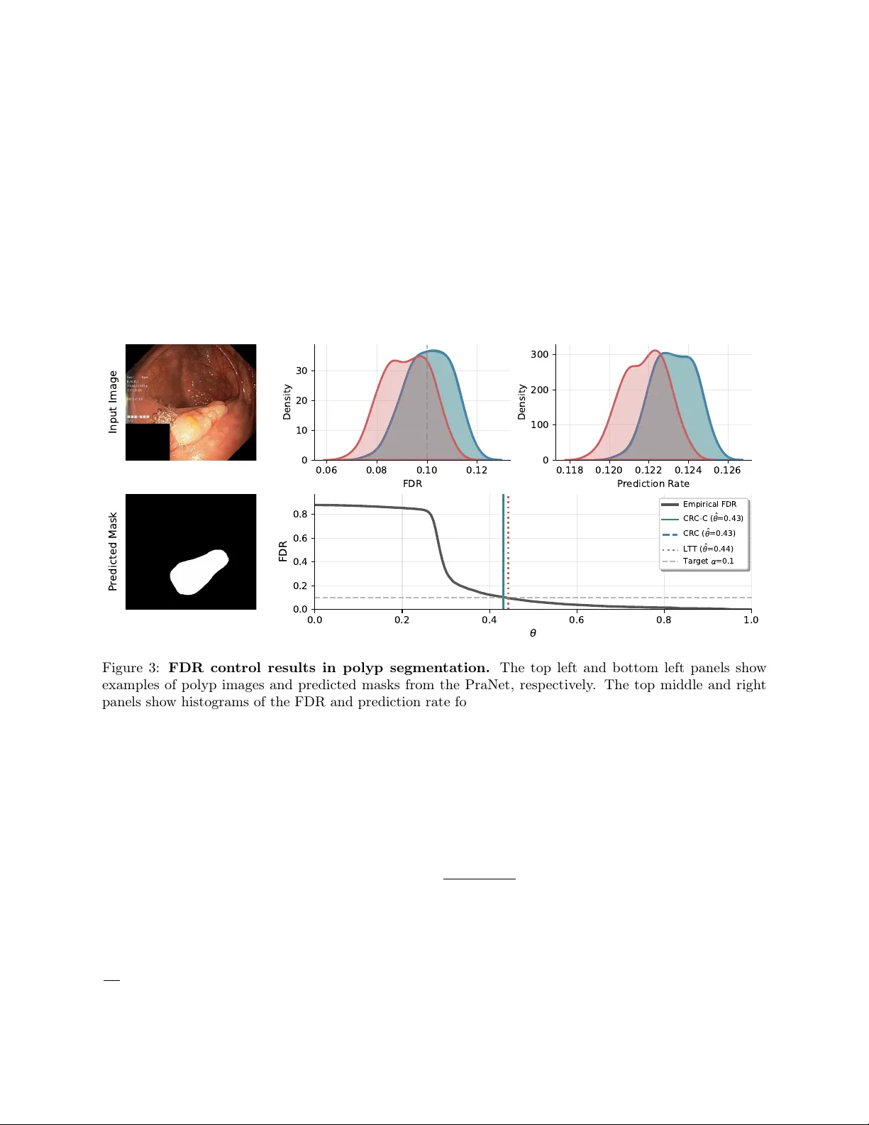
Conformal Risk Con trol for Non-Monotonic Losses Anastasios N. Angelop oulos Arena anastasios@arena.ai F ebruary 24, 2026 Abstract Conformal risk contro l is an extension of conformal prediction for controlling risk functions beyond misco verage. The original algorithm con trols the exp ected v alue of a loss that is monotonic in a one- dimensional parameter. Here, w e presen t risk con trol guaran tees for generic algorithms applied to p ossibly non-monotonic losses with multidimensional parameters. The guaran tees depend on the stability of the algorithm—unstable algorithms hav e lo oser guarantees. W e give applications of this technique to selectiv e image classification, FDR and IOU control of tumor segmen tations, and multigroup debiasing of recidivism predictions across ov erlapping race and sex groups using empirical risk minimization. 1 In tro duction Consider a sequence of random v ariables D 1: n +1 = (( X 1 , Y 1 ) , . . . , ( X n +1 , Y n +1 )) representing feature-lab el pairs with an exchangeable joint distribution. Let the first n datap oin ts, D 1: n , b e a kno wn calibration set, and last datap oin t, ( X n +1 , Y n +1 ) , represen t a test datap oin t whose lab el is unknown. Also define a b ounded loss, ℓ ( x, y ; θ ) ∈ [0 , 1] , which is a function of a datap oin t ( x, y ) and a parameter θ ∈ R d . Our goal is to select a parameter v alue ˆ θ using the calibration data D 1: n to b ound the exp ected loss on the test datap oint: E h ℓ ( X n +1 , Y n +1 ; ˆ θ ) i ≤ α, (1) where α ∈ [0 , 1] is user-sp ecified and the exp ectation is taken with resp ect to all n + 1 datap oints. W e call ( 1 ) a risk con trol guarantee. Conformal risk con trol, a generalization of conformal prediction [ GVV98 , V GS99 , V GS05 , LR W15 , LGR + 18 ] as developed in [ ABF + 24 ], handles the case where d = 1 and ℓ is monotonically nonincreasing in θ . Conformal risk con trol works by setting the parameter ˆ θ to b e ˆ θ = inf ( θ : 1 n + 1 n X i =1 ℓ ( X i , Y i ; θ ) ≤ α − 1 n + 1 ) , whic h is the smallest v alue of θ suc h that the empirical risk calculated on n + 1 datap oin ts is certain to b e b elow α . This pro vides the guarantee in ( 1 ) for monotonic losses, but can fail arbitrarily badly for non-monotonic losses, as sho wn in Prop osition 1 of [ ABF + 24 ]. In this paper, we give risk con trol guarantees for non-monotonic losses. The k ey insight is that the p opulation risk of ˆ θ dep ends on the stability of the algorithm for choosing ˆ θ —i.e., the change in risk when the test datap oin t is added to or remov ed from the calibration dataset. More formally , let A b e an algorithm mapping datasets to choices of θ and let D − i denote D 1: n +1 with the i th element remov ed. The parameter ˆ θ is the output of A ( D 1: n ) . W e say an algorithm A is β -stable with resp ect to a reference algorithm A ∗ and ℓ if E " 1 n + 1 n +1 X i =1 ℓ ( X i , Y i ; A ( D − i )) # ≤ E " 1 n + 1 n +1 X i =1 ℓ ( X i , Y i ; A ∗ ( D 1: n +1 )) # + β . The main theorem demonstrates that if an algorithm is stable with resp ect to a reference algorithm that con trols the risk when run on the full data, then the original algorithm also controls the risk. Here and throughout the pap er, we assume the algorithms are symmetric (i.e. permutation-in v ariant). 1 Theorem 1. Assume A is symmetric and β -stable with r esp e ct to A ∗ , that D 1: n +1 is exchange able, and that E [ ℓ ( X n +1 , Y n +1 ; A ∗ ( D 1: n +1 ))] ≤ α − β . Then E [ ℓ ( X n +1 , Y n +1 ; A ( D 1: n ))] ≤ α. Theorem 1 gives us an actionable workflo w for pro ducing risk-control algorithms. First, w e try to identify a reference algorithm, A ∗ , that controls the risk when applied on the full dataset of n + 1 datap oin ts. Then, w e try to approximate that algorithm via A , whic h runs only on n datap oin ts, and prov e that the difference in risks b et ween these tw o algorithms is lo w. The pro of of the main result is b elow. Pr o of. By exchangeabilit y and symmetry , E " 1 n + 1 n +1 X i =1 ℓ ( X i , Y i ; A ∗ ( D 1: n +1 )) # = E [ ℓ ( X n +1 , Y n +1 ; A ∗ ( D 1: n +1 ))] , and E " 1 n + 1 n +1 X i =1 ℓ ( X i , Y i ; A ( D − i )) # = E [ ℓ ( X n +1 , Y n +1 ; A ( D 1: n ))] . By β -stabilit y , E [ ℓ ( X n +1 , Y n +1 ; A ( D 1: n ))] ≤ E [ ℓ ( X n +1 , Y n +1 ; A ∗ ( D 1: n +1 ))] + β . Com bining this with the assumption that E [ ℓ ( X n +1 , Y n +1 ; A ∗ ( D 1: n +1 ))] ≤ α − β yields the result. Notice that Theorem 1 applies to θ in any space, and that b oundedness of ℓ w as nev er needed in the pro of of Theorem 1 . These concerns will come up later in determining stability b ounds, building on the literature on algorithmic stabilit y [ KR97 , BE02 , KN02 , MNPR06 , SSSSS10 , Y u13 , HRS16 , Y u17 , FV18 , BKZ20 , ZJ23 ]; see Chapter 13 of [ SSBD14 ] for a review of this extensive field. The notion of stability used herein is a form of leav e-one-out stability with resp ect to generic algorithms A and A ∗ ; we will prov e guarantees for a few differen t choices of algorithms dep ending on the setting. 1.1 Conformal Risk Con trol is Stable for Monotonic Losses Here we will show that the conformal risk control algorithm is stable for monotonic losses, and thus, satisfies the guaran tee in Theorem 1 . Prop osition 1. L et d = 1 , D b e any dataset, ℓ b e nonincr e asing in its last ar gument, A ( D ) = inf    θ : 1 | D | + 1 X ( x,y ) ∈ D ℓ ( x, y ; θ ) ≤ α − 1 | D | + 1    , and A ∗ ( D ) = inf    θ : 1 | D | X ( x,y ) ∈ D ℓ ( x, y ; θ ) ≤ α    . Then A is 0 -stable with r esp e ct to A ∗ . Pr o of. The b oundedness of ℓ and definition of A imply that for all i , 1 n + 1 n +1 X j =1 ℓ ( X j , Y j ; A ( D − i )) ≤ 1 n + 1 X j ∈ [ n +1] \ i ℓ ( X j , Y j ; A ( D − i )) + 1 n + 1 ≤ α. A ( D − i ) therefore satisfies the constraint in the definition of A ∗ ( D 1: n +1 ) , and the monotonicity of the loss giv es A ( D − i ) ≥ A ∗ ( D 1: n +1 ) . Therefore, ℓ ( X i , Y i ; A ( D − i )) ≤ ℓ ( X i , Y i ; A ∗ ( D 1: n +1 )) , and E " 1 n + 1 n +1 X i =1  ℓ ( X i , Y i ; A ( D − i )) − ℓ ( X i , Y i ; A ∗ ( D 1: n +1 ))  # ≤ 0 . Rearranging terms giv es 0 -stability . 2 Com bining Prop osition 1 with Theorem 1 exactly recov ers the classical conformal risk control guarantee. Corollary 1. The c onformal risk c ontr ol algorithm A define d in Pr op osition 1 satisfies E [ ℓ ( X n +1 , Y n +1 ; A ( D 1: n ))] ≤ α. Pr o of. F or monotonic losses, Prop osition 1 shows that the conformal risk control algorithm A is 0 -stable. Applying Theorem 1 with β = 0 recov ers the guarantee. The key takea w ay is that the pro of of conformal risk control’s v alidit y has t wo parts, which can b e decoupled: (1) pro ving monotonicit y implies stability , and (2) pro ving that stability implies risk control. Theorem 1 tells us that (2) holds for general algorithms. The remainder of the paper will b e dedicated to replacing step (1) with other stable algorithms, in the context of non-monotonic losses. Looking forward, Section 2 gives stability b ounds for classes of non-monotonic losses and shows how to estimate these stability b ounds for use in Theorem 1 . Section 3 sho ws exp erimental v alidation of these metho ds. 2 Metho ds 2.1 Setup and Notation Let X b e the feature space, Y b e the lab el space, and Z = X × Y . Datasets are ordered v ectors of feature-lab el pairs, denoted D ∈ Z ∗ , where the notation Z ∗ refers to the space of any-length sequences with elements in Z . A dataset D can ha ve rep eated entries; the size of the dataset is denoted as | D | . T o refer to the dataset of random v ariables used throughout this pap er, we will use the notation D 1: k = (( X 1 , Y 1 ) , . . . , ( X k , Y k )) = ( Z 1 , . . . , Z k ) . F urthermore, we use D − i to denote the dataset with the i th element remo ved. W e will let ˆ R D ( θ ) = 1 | D | P ( x,y ) ∈ D ℓ ( x, y ; θ ) denote the empirical risk, with the shorthand ˆ R 1: k ( θ ) = ˆ R D 1: k ( θ ) and ˆ R − i ( θ ) = ˆ R D − i ( θ ) . W e also denote the p opulation risk as R ( θ ) = E [ ℓ ( X n +1 , Y n +1 ; θ )] . Also, we will let ˆ θ k = A ( D 1: k ) and ˆ θ − i = A ( D − i ) for all k and i . When A is β -stable with resp ect to A and ℓ is clear from context, we will simply say it is β -stable. W e will also use the notation [ k ] = { 1 , . . . , k } for any p ositive in teger k . 2.2 Stable Algorithms This section describes three stable classes of risk control algorithms. W e b egin with the case of general b ounded losses, whic h we handle via discretization. Next, we give a stronger result for contin uous, Lipschitz losses with a strong crossing p oint at α . Finally , we perform a narrow case study with explicit constants: selectiv e classification, otherwise known as classification with abstention. By abstaining from prediction on the hardest examples, selective classification allows us to impro ve a mo del’s accuracy on the even t that it issues a prediction. Selective classification is one of the most imp ortan t applications of non-monotonic conformal risk control due to its ubiquitous practical utility in safe automation. Throughout this section, we will set d = 1 . 2.2.1 General Bounded Losses T o handle general losses b ounded in [0 , 1] , w e will use algorithms that discretize Θ to imp ose stability . First, let A ( D ) = inf { θ ∈ Θ m = { 0 , 1 m , 2 m , . . . , 1 } : ˆ R D ( θ ) ≤ α } for Θ = [0 , 1] and an y p ositive integer m . This is simply the discretized version of the previously studied algorithms. W e will assume nothing ab out the loss other than the existence of a safe solution, ℓ ( z ; 1) = 0 for all z ∈ X × Y . Prop osition 2. L et D 1: n +1 b e sample d i.i.d., Θ m = { 0 , 1 m , . . . , 1 } , ℓ ( · ; 1) = 0 , and define A ( D ) := inf  θ ∈ Θ m : ˆ R D ( θ ) ≤ α  . Then E  R ( ˆ θ n )  ≤ α + 1 2 √ n    s − W − 1  − 1 4 n ( m + 1) 2  + v u u t − 1 W − 1  − 1 4 n ( m +1) 2     = α + ˜ O  1 √ n  , 3 wher e W − 1 is the − 1 st br anch of the L amb ert W function and ˜ O denotes the gr owth r ate excluding lo garithmic factors. This prop osition tells us that we can achiev e risk control for general losses with the discretized algorithm up to a dominating factor of ˜ O  1 √ n  , since W − 1 is of logarithmic order. 2.2.2 Con tinuous, Lipsc hitz Losses Next, w e study the same ro ot-finding algorithm, A ( D ) = inf { θ ∈ R : ˆ R D ( θ ) ≤ α } , on losses that satisfy regularit y conditions. If the ro ot is leav e-one-out stable, meaning that removing a single datap oint do es not drastically c hange the lo cation of the ro ot, then for smo oth losses, the algorithm will control the risk. Prop osition 3. L et d = 1 , A ( D ) = inf { θ ∈ R : ˆ R D ( θ ) ≤ α } , and D 1: n +1 b e exchange able. L et ℓ b e c ontinuous and L -Lipschitz in θ , and assume that ˆ θ n +1 is almost sur ely finite. F urthermor e, assume ther e exist m, r > 0 such that ˆ R 1: n +1 ( θ ) ≤ α − m ( θ − ˆ θ n +1 ) ∀ θ ∈ [ ˆ θ n +1 , ˆ θ n +1 + r ] , ˆ R 1: n +1 ( θ ) ≥ α + m ( ˆ θ n +1 − θ ) ∀ θ ∈ [ ˆ θ n +1 − r, ˆ θ n +1 ] , and ˆ R 1: n +1 ( θ ) ≥ α + mr ∀ θ ∈ [ −∞ , ˆ θ n +1 − r ) (2) almost sur ely. Then if 1 n +1 < mr , A is L m ( n +1) -stable with r esp e ct to A ∗ ≡ A . This result sa ys that if the empirical risk satisfies: 1. lo cal linearity with sufficient slop e at its leftmost crossing of α , and 2. do es not come to o close to α after the leftmost crossing, then the risk is controlled. In tuitively , the risk cannot touch α in t wo highly disjoint regions, otherwise the selected parameter ma y b e unstable. Pr o of. Set ϵ := 1 / ( n + 1) . First, observe the following leav e-one-out bound: sup θ ∈ Θ | ˆ R − i ( θ ) − ˆ R 1: n +1 ( θ ) | ≤ ϵ. (3) Applying the assumptions in ( 2 ) giv es ˆ R 1: n +1  ˆ θ n +1 − δ  ≥ α + mδ and ˆ R 1: n +1  ˆ θ n +1 + δ  ≤ α − mδ ∀ δ ∈ (0 , r ] . Com bining the ab ov e displa y applied with δ = ϵ/m and the leav e-one-out b ound gives ˆ R − i  ˆ θ n +1 − δ  ≥ α + m ϵ m − ϵ = α, and ˆ R − i  ˆ θ n +1 + δ  ≤ α − m ϵ m + ϵ = α, implying that α ∈ h ˆ R − i  ˆ θ n +1 ± ϵ m i . Therefore, by contin uit y , ˆ R − i ( θ ) = α has a solution in I := h ˆ θ n +1 − ϵ m , ˆ θ n +1 + ϵ m i . Next, for an y θ ∈ [ ˆ θ n +1 − r, ˆ θ n +1 − ϵ/m ) ( 2 ) combines with ( 3 ) to yield ˆ R − i ( θ ) ≥ α + m ( ˆ θ n +1 − θ ) − ϵ > α, so there is no ro ot of ˆ R − i ( θ ) = α in that in terv al. F or θ < ˆ θ n +1 − r , the second assumption in ( 2 ) com bines with ( 3 ) to giv e ˆ R − i ( θ ) ≥ α + mr − ϵ > α, 4 so there is no ro ot to the left of ˆ θ n +1 − r either. Hence the leftmost ro ot of ˆ R − i ( θ ) − α lies in I , and therefore   ˆ θ − i − ˆ θ n +1   ≤ ϵ m = 1 m ( n + 1) . Finally , since ℓ ( · ; θ ) is L -Lipschitz in θ , ℓ  Z i ; ˆ θ − i  ≤ ℓ  Z i ; ˆ θ n +1  + L   ˆ θ − i − ˆ θ n +1   ≤ ℓ  Z i ; ˆ θ n +1  + L m ( n + 1) . A v eraging ov er i = 1 , . . . , n + 1 and taking exp ectations on b oth sides completes the pro of. Com bining the previous result with Theorem 1 gives a risk-control result. Corollary 2. Under the same c onditions as Pr op osition 3 , A satisfies E h R ( ˆ θ n ) i ≤ α + L m ( n + 1) . 2.2.3 Selectiv e Classification Finally , we give stability guarantees for selective classification. Let ˆ Y i represen t a prediction of Y i and ˆ P i ∈ [0 , 1] represent a confidence in this prediction. Both ˆ Y i = ˆ y ( X i ) and ˆ P i = ˆ p ( X i ) are outputs of deterministic mo dels run on X i . W e seek a confidence threshold ˆ θ satisfying P ( ˆ Y n +1  = Y n +1 | ˆ P n +1 > ˆ θ ) ≤ α. As describ ed in [ ABC + 25 ], this is equiv alen t to asking that E h 1 n ˆ Y n +1  = Y n +1 and ˆ P n +1 > ˆ θ o − α 1 n ˆ P n +1 > ˆ θ o + α i = E h ℓ ( Z n +1 ; ˆ θ ) i ≤ α, where ℓ ( x, y ; θ ) = 1 { ˆ y ( x )  = y and ˆ p ( x ) > θ } − α 1 { ˆ p ( x ) > θ } + α . Notably , ℓ is a non-monotonic loss. W e will study the b elo w algorithm A for selective classification, A ( D ) = inf n θ : ˆ R D ( θ ) ≤ α o , (4) whic h simply chooses the smallest v alue of θ that controls the risk. First, we characterize the stability of this selective classification algorithm. Let the ˆ P i b e distinct almost surely . Let the vector V denote the inv erse sorting p erm utation of ˆ P , so that ˆ P i = ˆ P ( V i ) , where the notation ˆ P ( j ) represen ts the j th smallest v alue of ˆ P . F urther, let V = = { V i : ˆ Y i = Y i } , V  = = { V i : ˆ Y i  = Y i } . The core idea is that each loss is piecewise constant, with one component corresp onding to when the algorithm is abstaining and another when it issues a prediction. Thus it only has one change p oin t, exactly at the lo cation of ˆ P i : ℓ ( Z i ; θ ) = 1 − (1 − α ) 1 n θ ≥ ˆ P i o ∀ i ∈ V  = , and (5) ℓ ( Z i ; θ ) = α 1 n θ ≥ ˆ P i o ∀ i ∈ V = . Because the losses are righ t-contin uous and piecewise constan t with jumps at ˆ P , we are guaranteed that if D is a sub dataset of D 1: n +1 , then A ( D ) = ˆ P ( j ) for some j . Along these lines, define ˆ ȷ n +1 and ˆ ȷ − i as ˆ P (ˆ ȷ n +1 ) = ˆ θ n +1 and ˆ P (ˆ ȷ − i ) = ˆ θ − i . W e will use this index-space characterization to b ound the stability . Prop osition 4. The sele ctive classific ation algorithm in ( 4 ) is β -stable with β = 2 max { α, 1 − α } E [ K ] n + 1 , wher e K = max i | ˆ ȷ − i − ˆ ȷ n +1 | . 5 Pr o of. By ( 5 ), it suffices to pro ve that, almost surely , n +1 X i =1  ℓ ( X i , Y i ; A ( D − i )) − ℓ ( X i , Y i ; A ∗ ( D 1: n +1 ))  = X i ∈ [ n +1] w i ∆ i ≤ 2 max { α, 1 − α } K, where ∆ i = 1 n A ( D − i ) ≥ ˆ P i o − 1 n A ∗ ( D 1: n +1 ) ≥ ˆ P i o and w i = α for i ∈ V = and − (1 − α ) otherwise. W e can b egin by rewriting the ∆ i terms as ∆ i = 1 n A ( D − i ) ≥ ˆ P i > A ( D 1: n +1 ) o − 1 n A ( D − i ) < ˆ P i ≤ A ( D 1: n +1 ) o = 1 { ˆ ȷ − i ≤ V i < ˆ ȷ n +1 } − 1 { ˆ ȷ − i > V i ≥ ˆ ȷ n +1 } . Note th at the tw o ev ents inside the indicators are mutually exclusiv e, and corresp ond to the “crossin g” of A ( D − i ) o ver ˆ P i in the do wnw ard or upw ard directions. Therefore, X i ∈ [ n +1] w i ∆ i ≤ max { α, 1 − α } X i ∈ [ n +1] | ∆ i | ≤ max { α, 1 − α } |{ i : ˆ ȷ − i ≤ V i < ˆ ȷ n +1 or ˆ ȷ − i > V i ≥ ˆ ȷ n +1 }| . (6) Define the index sets S − :=  i ∈ [ n +1] : ˆ ȷ − i ≤ V i < ˆ ȷ n +1  and S + :=  i ∈ [ n +1] : ˆ ȷ − i > V i ≥ ˆ ȷ n +1  . Then the set of indices that contribute nonzero terms to P i ∈ [ n +1] | ∆ i | is S := S − ∪ S + , and S − ∩ S + = ∅ b y definition. By the definition of K = max i | ˆ ȷ − i − ˆ ȷ n +1 | , for ev ery i ∈ S − w e hav e 1 ≤ ˆ ȷ n +1 − V i ≤ ˆ ȷ n +1 − ˆ ȷ − i ≤ | ˆ ȷ − i − ˆ ȷ n +1 | ≤ K , hence V i ∈ { ˆ ȷ n +1 − K , . . . , ˆ ȷ n +1 − 1 } ∩ { 1 , . . . , n +1 } . Similarly , for every i ∈ S + w e hav e ˆ ȷ n +1 ≤ V i ≤ ˆ ȷ − i − 1 ≤ ˆ ȷ n +1 + K − 1 , i.e. V i ∈ { ˆ ȷ n +1 , . . . , ˆ ȷ n +1 + K − 1 } ∩ { 1 , . . . , n +1 } . Because the V i ’s are distinct (the map i 7→ V i is a p erm utation of { 1 , . . . , n + 1 } ), at most one index i can corresp ond to each admissible v alue of V i . Therefore, | S − | ≤ K and | S + | ≤ K , whic h, since | ∆ i | ≤ 1 for all i , yields X i ∈ [ n +1] | ∆ i | ≤ | S | ≤ | S − | + | S + | ≤ 2 K . Com bining this with ( 6 ) yields X i ∈ [ n +1] w i ∆ i ≤ max { α, 1 − α } | S | ≤ 2 max { α, 1 − α } K, as claimed. The ab ov e result gives a simple, distribution-free c haracterization of the stability of the selective classifica- tion algorithm. It is then relativ ely easy to estimate E [ K ] with the b o otstrap—i.e., drawing samples from the empirical distribution, computing K on these samples, and taking the av erage. When combined with Theorem 1 , this stabilit y result implies a selective accuracy b ound. 6 1 100 200 300 400 500 j 0.0 0.2 0.4 0.6 0.8 1.0 Error ( + 1 j , + 2 j ] E j ( w e l l - r a n k e d ) E j ( p o o r l y - r a n k e d ) E j ( p o o r l y - r a n k e d , a d v e r s a r i a l ) Figure 1: Cum ulative a verage error ¯ E j for three scenarios alongside the shrinking interv al ( α + (1 − α ) /j, α + (2 − α ) /j ] from Prop osition 5 , with α = 0 . 25 and n = 500 . In eac h case E i ∼ Bernoulli ( p i ) indep enden tly . In the well-rank ed case, p i = max (0 , 2 α (1 − ( i − 1) /m )) , m = ( n + 1) / 2 , a linear decay from 2 α to 0 at the midp oin t, so that ¯ E j crosses b elo w α in the second half and even tually exits the interv al. In the p o orly rank ed case, p i = 0 . 35 for all i ; the constant rate exceeds α , and ¯ E j remains ab ov e the interv al. In the p o orly rank ed adversarial case, p i = α for all i ; the av erage concentrates near α but stays b elow the interv al as it shrinks to ward α from ab o ve. The blue band is the interv al; the gray dotted line marks α . K is the num b er of j for whic h ¯ E j lands inside the in terv al. Corollary 3. L et D 1: n +1 b e exchange able. Then the sele ctive classific ation algorithm in ( 4 ) satisfies P ( ˆ Y n +1 = Y n +1 | ˆ P n +1 > ˆ θ n ) ≥ 1 − α − 2 max { α, 1 − α } E [ K ] n + 1 . Ho wev er, the question remains as to a more explicit c haracterization of E [ K ] . The following prop osition giv es an answer, saying that the exp ected v alue of K is b ounded by the n umber of times the algorithm’s running error rate crosses a thin band around α , as visualized in Figure 1 . Prop osition 5. In the same setting as Pr op osition 4 , define ¯ E j = 1 j P i ≤ j E i , wher e E =  1 n ˆ Y V 1  = Y V 1 o , . . . , 1 n ˆ Y V n +1  = Y V n +1 o Then E [ K ] ≤ n +1 X j =1  P  ¯ E j ∈  α + 1 − α j , α + 2 − α j  . Because in practical settings we use mo dels that tend to ha ve a reasonable ranking, w e therefore exp ect K to b e small in practice, as in Figure 1 . This in tuition can b e further formalized by applying a concen tration b ound like Hoeffding’s inequality on ¯ E j to bound the probability it lies in  α + 1 − α j , α + 2 − α j  conditionally on the vector ˆ P . The v alidity of such an argumen t hinges on the fact that the co ordinates of E are indep enden t Bernoulli random v ariables with different means after conditioning on ˆ P ; the result is not to o in terpretable, so w e omit it here. Pr o of. W e keep the same notation as in the pro of of Prop osition 4 , and notice that K = max i |A ′ ( D − i ) − A ′ ( D 1: n +1 ) | , 7 with ˆ ȷ n +1 = A ′ ( D 1: n +1 ) = max    j : X v ∈ V = α 1 { j ≤ v } + X v ∈ V  = (1 − (1 − α ) 1 { j ≤ v } ) ≤ ( n + 1) α    = max  j ∈ { 0 , . . . , n + 1 } : 1 + T j ≥ 0  , where T j = P i ≤ j w i = − P i ≤ j E i + j α . The leav e-one-out index ˆ ȷ − i = A ′ ( D − i ) is defined similarly , with V = − i in place of V = , V  = − i in place of V  = , and n in place of n + 1 . Therefore, K dep ends on the v alues of ˆ P 1 , . . . , ˆ P n +1 , only through the error vector E (whic h itself only dep ends on their order). If we delete the datap oin t at index V i , then for all j ≥ V i the new partial sums shift b y a constant: T − i j = T j +1 − α if E i = 0 , T − i j = T j +1 + (1 − α ) if E i = 1 . Hence remo ving a correct point ( E i = 0 ) can only inv alidate those j ≥ V i for whic h 1 + T j +1 ∈ [0 , α ) , and removing an error ( E i = 1 ) can only create feasibility for those j ≥ V i with 1 + T j +1 ∈ [ − (1 − α ) , 0) . Consequen tly , K ≤   { j ∈ [ n ] : T j ∈ [ − 1 , α − 1) }   +   { j ∈ [ n ] : T j ∈ [ α − 2 , − 1) }   =   { j ∈ [ n ] : T j ∈ [ α − 2 , α − 1) }   W e can b ound this quantit y in exp ectation as E [ K ] ≤ E    { j ∈ [ n ] : T j ∈ [ α − 2 , α − 1) }    = E   n +1 X j =1 1 { α − 2 ≤ T j < α − 1 }   = n +1 X j =1 P ( T j ∈ [ α − 2 , α − 1)) = n +1 X j =1 P  ¯ E j ∈  α + 1 − α j , α + 2 − α j  . 2.3 Guaran tees for Empirical Risk Minimization So far, we hav e studied ro ot-finding algorithms that select the most extreme p oin t satisfying an inequalit y . Here, w e will instead study regularized empirical risk minimization (ERM) algorithms: A ( D ) = argmin θ ∈ R d ˆ R D ( θ ) + λ 2 ∥ θ ∥ 2 2 , for some regularization lev el λ ≥ 0 . W e will let ℓ : R d → R b e p oten tially unbounded, and d ≥ 1 . W e will sho w tw o types of guaran tees with resp ect to ERM. First, we prov e guarantees on the generalization gap: the gap b etw een the risk of the empirical risk minimizer with resp ect to an oracle quantit y , such as the full-data or p opulation risk minimizers. Second, w e prov e stability b ounds on the first-order optimalit y condition; i.e., ho w close the p opulation gradient is to zero. 2.3.1 Risk Control Guarantees on the Loss First, w e show the stability of ERM on the scale of the loss. Prop osition 6. L et Θ = R d , ℓ b e c onvex in θ , and assume ther e exists ρ : Z → [0 , ∞ ) such that for al l z ∈ Z and θ , θ ′ ∈ R d , | ℓ ( z ; θ ) − ℓ ( z ; θ ′ ) | ≤ ρ ( z ) ∥ θ − θ ′ ∥ 2 . (7) Then A is β -stable with β ≤ 2 E [ ρ ( Z n +1 ) 2 ] λ ( n + 1) . This result can b e used in conjunction with Theorem 1 to give a generalization guarantee on ERM, as b elo w. 8 Corollary 4. In the setting of Pr op osition 6 , E h ℓ ( X n +1 , Y n +1 ; ˆ θ n ) + λ 2 ∥ ˆ θ n ∥ 2 2 i ≤ R ∗ + 2 E [ ρ ( Z n +1 ) 2 ] λ ( n + 1) , wher e R ∗ = min θ ∈ Θ E [ ℓ ( X n +1 , Y n +1 ; θ ) + λ 2 ∥ θ ∥ 2 2 ] . These results represen t minor v ariations on the canonical results in Section 5 of [ BE02 ]. 2.3.2 Risk Control Guarantees on the Gradient Next, w e address stability of the exp ected gradien t. Building to wards this, we will need a m ultiv ariate notion of stabilit y to handle gradients when d > 1 : an algorithm A is β -stable with resp ect to A ∗ and g if E " 1 n + 1 n +1 X i =1 g ( X i , Y i ; A ( D − i )) # ⪯ E " 1 n + 1 n +1 X i =1 g ( X i , Y i ; A ∗ ( D 1: n +1 )) # + β , where β ∈ R d , and ⪯ represen ts the standard partial ordering on v ectors (i.e., the inequality holds comp onent- wise). Theorem 1 also has an extension to d > 1 , which we present b elow. Theorem 2. Assume A is symmetric and β -stable with r esp e ct to A ∗ and g , that D 1: n +1 is exchange able, and that E [ g ( X n +1 , Y n +1 ; A ∗ ( D 1: n +1 ))] ⪯ α − β . Then E [ g ( X n +1 , Y n +1 ; A ( D 1: n ))] ⪯ α. The pro of of this theorem is iden tical to that of Theorem 1 , except with ⪯ in place of ≤ . Now we proceed with the stability result, stated b elo w for differentiable con vex losses. The differentiabilit y is not needed, and is only used to simplify the statemen t and pro of of the prop osition. Prop osition 7. Assume ℓ is a c onvex, differ entiable function of θ and that ther e exists a me asur able function ρ : Z → [0 , ∞ ) such that for al l θ , θ ′ ∈ R d and almost al l z ∈ Z , ∥∇ ℓ ( z ; θ ) − ∇ ℓ ( z ; θ ′ ) ∥ 2 ≤ ρ ( z ) ∥ θ − θ ′ ∥ 2 . Assume also that ˆ R 1: n +1 is µ -str ongly c onvex for some µ ∈ [0 , ∞ ) (noting that µ = 0 is also al lowable, so it ne e d not b e str ongly c onvex). Then the r e gularize d ERM algorithm A is β -stable with r esp e ct to ∇ ℓ , wher e β = E [ ρ ( Z n +1 ) ∥∇ ℓ ( Z n +1 ; ˆ θ n ) ∥ 2 ] + E h ρ ( Z n +1 ) ∥ 1 n P n j =1 ∇ ℓ ( Z j ; ˆ θ n ) ∥ 2 i ( µ + λ )( n + 1) 1 d . Eliding the Lipsc hitz constant ρ ( Z n +1 ) , this result tells us that ERM is stable with β = E [ magnitude of test gradien t ] + E [ magnitude of training gradien t ] ( µ + λ )( n + 1) . Under normal circumstances, b oth terms in the n umerator will b e constan t-order, and the latter term will b e near-zero (in fact, when λ = 0 , it is exactly zero). Prop osition 7 also holds for nondifferentiable losses, replacing every gradient in β with a supremum ov er all subgradients in the sub differential at ˆ θ n ; the pro of of this more general result is morally the same, so w e omit it. The assumption that ˆ R 1: n +1 is strongly con vex is w eaker than strong conv exity of the loss function itself, and allo ws for, e.g., ordinary least squares with a full-rank design matrix, ev en though the individual losses may not b e strongly conv ex. Com bining Prop osition 7 with Theorem 2 gives a multi-dimensional risk control b ound, as b elo w. Corollary 5. In the same setting as Pr op osition 7 , we have that E h ∇ ℓ ( X n +1 , Y n +1 ; ˆ θ n ) i ⪯ β − λ E [ ˆ θ n ] . 9 This tells us the risk is con trolled up to β plus a term to handle regularization. Finally , w e present an adjusted algorithm that achiev es a conserv ativ e risk con trol guarantee on the gradien t. Let e A γ ( D ) = argmin θ ∈ R d ˆ R D ( θ ) + λ 2 ∥ θ ∥ 2 2 + γ 1 ⊤ d θ . The final term, γ 1 ⊤ d θ , has gradient γ 1 d , pushing all comp onen ts of the solution in the negative direction to comp ensate, while retaining conv exity . A careful selection of γ to balance terms can therefore yield risk con trol. Prop osition 8. In the same setting as Pr op osition 7 , we have that E h ∇ ℓ ( X n +1 , Y n +1 ; ˆ θ n ) i ⪯ β γ − λ E [ ˆ θ n ] − γ 1 d , wher e β γ = E [ ρ ( Z n +1 ) ∥∇ ℓ ( Z n +1 ; ˆ θ n ) ∥ 2 ] + E [ ρ ( Z n +1 )]  E h ∥ 1 n P n j =1 ∇ ℓ ( Z j ; ˆ θ n ) ∥ 2 i + 2 γ  ( µ + λ )( n + 1) 1 d . F urthermor e, pr ovide d n > 2 µ + λ E [ ρ ( Z n +1 )] − 1 , ther e exists an explicit choic e of γ that gives E h ∇ ℓ ( X n +1 , Y n +1 ; ˆ θ n ) i ⪯ 0 . These gradien t b ounds allow us to pro ve distribution-free multigroup risk control guarantees for ERM. These guaran tees are in the style of [ GCC23 ] and [ BAJB24 ], which handle the sp ecial cases of the quan tile loss [ KB78 ] and monotonic losses in d = 1 resp ectiv ely , and b oth of whic h only give full-conformal type guarantees that require having access to the test co v ariate X n +1 and p otentially lo oping through all p ossible test lab els y ∈ Y . Herein, w e allo w a more general class of non-monotonic losses, a high-dimensional θ , and also give split- conformal versions of these tec hniques that do not dep end on the test cov ariate or lab el. Dep ending on the form of the gradien t, these guarantees can recov er multiv alidit y guarantees [ BGJ + 22 , JNRR22 ] or m ultiaccuracy guaran tees [ KGZ19 ], and are also related to the literature on multicalibration [ HJKRR18 , DDZ23 , NR23 ]. The first example sho ws how we can p ost-pro cess a black-box mo del to achiev e multigroup unbiasedness using ordinary least squares. F or this purp ose, define X n +1 = ( X 1 , . . . , X n +1 ) ⊤ and λ min as the minimum eigen v alue function. Corollary 6. L et X = { 0 , 1 } d , f : X → R b e any fixe d function, ℓ ( x, y ; θ ) = 1 2 ∥ f ( x ) + x ⊤ θ − y ∥ 2 2 , and A ( D ) = argmin θ ∈ R d 1 | D | P ( x,y ) ∈ D ℓ ( x, y ; θ ) . Assume also that λ min ( X n + 1 ⊤ X n + 1 / ( n + 1)) ≥ µ > 0 almost sur ely. Then for al l j ∈ [ d ] , E [ Y n +1 | X n +1 ,j = 1] ∈ E [ f ( X n +1 ) + X ⊤ n +1 ˆ θ n | X n +1 ,j = 1] ± d 3 2 E [ | f ( X n +1 ) + X ⊤ n +1 ˆ θ n − Y n +1 | ] µ ( n + 1) P ( X n +1 ,j = 1) ! . If X n +1 represen ts a vector of group membership indicators, the adjusted prediction f ( X n +1 ) + X ⊤ n +1 ˆ θ n is appro ximately unbiased for all groups simultaneously , so long as they hav e sufficient probability of b eing observ ed. This is essentially the batch v ersion of the gradient equilibrium guarantees in [ AJT25 ]. Much lik e in the case of gradient equilibrium, Corollary 5 extends to all generalized linear mo dels, not just linear regression, and w e omit the pro of b ecause it is essen tially identical. 2.4 Estimating the Stabilit y Parameter Here, w e seek to estimate upp er bounds on the stability parameter. W e will do so using the calibration sample, and a veraging across b o otstrap replicates. Let ˆ P n b e the empirical measu re on D 1: n = { Z i = ( X i , Y i ) } n i =1 . F or b = 1 , . . . , B , dra w a b o otstrap dataset D ( b ) =  Z ( b ) 1 , . . . , Z ( b ) n +1  ∼ ˆ P n +1 n , 10 compute the estimate of β on D ( b ) , and a verage the bo otstrapp ed results. In well-behav ed circum- stances [ vdVW96 ], the b o otstrap mean consistently estimates the corresp onding p opulation exp ectation, and w e find this to b e the case in our exp erimen ts. That said, the v alidity of the b o otstrap under subsampling is not trivial [ PR W99 ] and represents an interesting av enue for further in vestigation. The tightest wa y to estimate β is directly from its definition, as opp osed to applying the b ounds from earlier in Section 2 . Fix a reference algorithm A ∗ (as in Theorem 1 ). F or eac h bo otstrap dataset D ( b ) compute ∆ ( b ) := 1 n + 1 n +1 X i =1 h ℓ  Z ( b ) i ; A ( D ( b ) − i )  − ℓ  Z ( b ) i ; A ∗ ( D ( b ) )  i . W e estimate β by the p ositiv e part of the b o otstrap mean b β def :=  ∆  + , ∆ = 1 B B X b =1 ∆ ( b ) . 3 Exp erimen ts This section p erforms exp erimen ts to v alidate our method in sev eral practical setups. First, w e run a real-data selectiv e classification exp erimen t on the Imagenet dataset. Next, we run FDR and IOU control exp eriments on tumor segmen tation. Finally , we run a multigroup debiasing exp erimen t of recidivism predictions. Co de to repro duce the exp eriments is av ailable at https://github.com/aangelopoulos/nonmonotonic- crc . W e run exp erimen ts with three meth ods. The first, which we call CRC-C, is the conserv ative version of conformal risk control, run at an adjusted level α ′ = α − b β def , where b β def is the estimated algorithmic stabilit y from Section 2.4 via the b o otstrap. The second, which we simply call CRC, is the unadjusted version of conformal risk control, i.e., ( 4 ) with α set to b e the desired risk level. Finally , we run the Learn-then-T est pro cedure from [ ABC + 25 ], whic h provides a distribution-free guarantee that P  E h ℓ ( X n +1 , Y n +1 ; ˆ θ )   D 1: n i ≤ α  ≥ 1 − δ, where here we choose δ = 0 . 1 . In all the experiments b elow, L TT tends to b e more conserv ative than CRC and CRC-C, which is exp ected giv en that it is a high-probability guarantee. Nonetheless, we include it as the standard baseline for non-monotonic risk con trol, and as a contrast to our exp ectation control metho d. 3.1 Selectiv e Classification: Imagenet 0.0 0.2 0.4 0.6 0.8 1.0 0.7 0.8 0.9 1.0 Selective A ccuracy 0.00 0.25 0.50 0.75 1.00 P r ediction R ate 0 2 4 6 Density 0.85 0.90 0.95 1.00 Selective A ccuracy 0 5 10 15 Density A ccuracy CR C-C CR C L T T 1 = 0 . 9 Figure 2: Selectiv e classification results on Imagenet. The left panel shows the c hoices of thresholds from CR C, CRC-C, and L TT sup erimp osed with the p opulation accuracy curv e. The middle panel sho ws a k ernel density estimate of the prediction rate for all three metho ds ov er 100 resamplings of the data. The righ t panel shows a similar plot for the selective accuracy . The Imagenet [ DDS + 09 ] experiment follows the same setting as in [ AB23 ]: w e use a ResNet-152 [ HZRS16 ] as the base classifier, and the highest predicted probability from the mo del is used as ˆ P i for each sample i . 11 The corresp onding ˆ Y 1 , . . . , ˆ Y n +1 represen t class lab el predictions, and Y 1 , . . . , Y n +1 represen t the true lab els. W e set n = 1000 . T o assess the algorithms’ p erformance, we display the thresholds chosen by all three algorithms and the resulting selective accuracy and prediction rate in Figure 2 . The ideal algorithm issues as many predictions as p ossible sub ject to the accuracy constraint; that is, it should generally meet the accuracy constraint exactly , and maximize the prediction rate. CRC is the least conserv ative, L TT is the most (as it is a high-probability guaran tee), and CRC-C is in the middle. The estimated stability parameter is β = 0 . 006 , meaning CRC is essen tially safe to use with no correction in this sp ecific example. Without correction, CRC is sligh tly lib eral, with an accuracy a hair b elo w 90% . CR C-C lands slightly ab ov e, while L TT is highly conserv ative and also higher v ariance. 3.2 Smo oth Losses: FDR in T umor Segmentation Input Image P r edicted Mask 0.06 0.08 0.10 0.12 FDR 0 10 20 30 Density 0.118 0.120 0.122 0.124 0.126 P r ediction R ate 0 100 200 300 Density 0.0 0.2 0.4 0.6 0.8 1.0 0.0 0.2 0.4 0.6 0.8 FDR Empirical FDR C R C - C ( = 0 . 4 3 ) C R C ( = 0 . 4 3 ) L T T ( = 0 . 4 4 ) T a r g e t = 0 . 1 Figure 3: FDR con trol results in p olyp segmen tation. The top left and b ottom left panels sho w examples of p olyp images and predicted masks from the PraNet, resp ectiv ely . The top middle and right panels show histograms of the FDR and prediction rate for CRC-C, CRC, and L TT, ov er 100 resamplings of the data, respectively . Notice that CRC and CRC-C ov erlap almost en tirely . The bottom righ t panel sho ws selections of ˆ θ made b y the three metho ds on the calibration data sup erimp osed with the true FDR calculated o ver the whole dataset. Next, w e handle false discov ery rate [ BH95 ] (FDR) con trol on the PraNet [ FJZ + 20 ] p olyp segmentation task from [ AB23 ]. Each image X i is a d × d grid of pixels, and each lab el Y i is a d × d binary grid, with ‘1‘ signifying the presence of a tumor. The predictive model, f ( X i ) ∈ [0 , 1] , outputs a probabilit y that each pixel con tains a tumor, which w e binarize at level θ to form ˆ y ( x ; θ ) . There are 1798 examples total in the dataset. The FDR loss is then ℓ ( x, y ; θ ) = 1 − | y ⊙ ˆ y ( x ; θ ) | | ˆ y ( x ; θ ) | , where the notation | y | represen ts the sum ov er all v alues in y and ⊙ represen ts the element-wise pro duct. The FDR is non-monotonic in θ , since b oth the numerator and denominator grow as θ shrinks. Ho wev er, it tends to b e a smo oth and well-behav ed loss function. W e generally seek to maximize discov eries sub ject to our FDR constrain t, so w e pick the largest set (smallest θ ) that controls our risk: A ( D ) = inf { θ : 1 | D | P ( x,y ) ∈ D ℓ ( x, y ; θ ) ≤ α } . Figure 3 shows empirical results from the FDR segmentation task with n = 500 . Over 1000 b o otstrap replicates, we found β ≈ 0 . 00007 for this task, indicating that correction is not needed for essentially any 12 0.81 0.82 0.83 0.84 IOU 0 20 40 60 80 Density 0.48 0.49 0.50 0.51 0.52 0 10 20 30 40 50 60 Density 0.0 0.2 0.4 0.6 0.8 1.0 0.0 0.2 0.4 0.6 0.8 1.0 1 - IOU IOU L oss E R M ( = 0 . 4 9 ) A chieved L oss: 0.172 Figure 4: IOU con trol results in p olyp segmen tation. The left and middle panels show histograms of the IOU and segmentation parameter θ for ERM ov er 100 resampl ings of the data, resp ectiv ely . The righ t panel sho ws the selection of ˆ θ sup erimposed with the true IOU calculated ov er the whole dataset. practical purp ose due to the regularity of this loss function. The results b ear this out, with the results of CR C-C and CRC ov erlapping almost entirely , and L TT b eing more conserv ative. 3.3 ERM Loss Guaran tees: IOU in T umor Segmen tation Next, w e handle intersection-o ver-union (IOU) control in the same tumor segmentation setting as Section 3.2 . The IOU is a measure of ov erlap common in the image segmentation literature, defined as the cardinality of the intersection of tw o segmentation masks divided by the cardinalit y of their union. In the p erfect case, the IOU is 1, but it can degrade if the masks do not p erfectly o verlap. Ideally , w e wan t to maximize the IOU, making this problem a go od candidate for empirical risk minimization. W e formally define the IOU loss function as ℓ ( x, y ; θ ) = 1 − | y ⊙ ˆ y ( x ; θ ) | | max( y , ˆ y ) | , where the denominator denotes the cardinality of the element-wise maximum. Our algorithm A minimizes the empirical risk with resp ect to this loss. Results in Figure 4 indicate that the ERM pro cedure achiev es an approximate minimizer. W e calculated β = 0 . 000056 for this problem ov er 100 b o otstrap iterations. 3.4 ERM Gradien t Guaran tees: Multigroup Debiasing of Recidivism Predictions Finally , we use the ERM algorithm to issue unbiased recidivism predictions ov er racial groups and sexes on the Correctional Offender Managemen t Profiling for Alternative Sanctions (COMP AS) Recidivism and Racial Bias dataset [ ALMK22 ], similarly to [ AJT25 ]. F o cusing on arrest records from Brow ard Count y , Florida, this dataset trac ks demographic details and criminal backgrounds alongside COMP AS-generated recidivism risk scores. These scores are utilized to inform pretrial bail decisions, but the errors exhibit significant racial disparities. The lab els Y i ∈ { 0 , 1 } are binary indicators of recidivism. The cov ariates X i ∈ { 0 , 1 } 5 are a v ector of indicators for each group: Blac k, White, Hispanic, Male, and F emale, resp ectively . Note that these groups o verlap. The predicted recidivism rate f i is obtained by taking the COMP AS recidivism score, which lies on an in teger scale from 1 to 10, and dividing it by 10. W e prepro cess the dataset to remo ve rare groups, and only consider the Caucasian, African-American, and Hispanic subgroups along with Male and F emale sexes. W e take n = 1000 from th e full dataset of 6787 samples. W e aim to recalibrate f i with a regression as in Corollary 6 . W e do this by running a p ost-ho c conserv ative OLS on the residual of the COMP AS predictor (with an optional linear term to pro vide a conserv ative guaran tee): i.e., taking A to b e ERM with ℓ ( z ; θ ) = 1 2  x ⊤ θ − ( y − f )  2 + β 1 ⊤ 5 θ . 13 0.10 0.05 0.00 0.05 0.10 0.15 Bias African-American Caucasian Hispanic Female Male Group Method Original Standard OLS Conservative OLS Figure 5: Results of m ultigroup debiasing on COMP AS dataset. Each row is a group, and the horizon tal axis shows the amoun t of predictive bias. Each violin plot shows the bias ov er 100 resamplings of the data for eac h metho d. The implied guarantee says that the adjusted predictions, f i + X ⊤ i ˆ θ n , are unbiased for all races and sexes, as stated in Corollary 6 . W e conduct exp eriments ev aluating the bias in Figure 5 using three metho ds: the ra w COMP AS predictor, the standard OLS with no linear term, and the conserv ative OLS including the linear term. In this case, β = 0 . 001839 , so there is almost no adjustment needed in this sp ecific example. The figure sho ws that the metho d effectively ensures all groups are unbiased. 4 Discussion This pap er sho wed that the v alidity of conformal risk con trol can b e viewed as a consequence of algorithmic stabilit y , and that therefore, all stable algorithms b enefit from conformal guarantees. This expands the scop e of the field, allowing us to prov e distribution-free b ounds for arbitrary tasks. Finding suc h tasks and corresp onding guarantees would b e an exciting av enue for future work. The insigh ts in this work also extend to full-conformal-t yp e algorithms (see [ V GS05 ] and the extension to risk con trol in [ Ang24 ]). The main difference is that the definition of stability b ecomes lea ve-one-label- out, as opp osed to leav e-one-datap oint-out, and the algorithm can therefore in volv e imputing the missing lab el. Otherwise, the main idea is the same. Similarly , the technique extends readily to non-exc hangeable distributions (see [ TBCR19 , BCR T22 ] and Chapter 7 of [ ABB24 ] for a review) via weigh ted exchangeabilit y . W e leav e further exploration of these imp ortan t themes to future work. It is also worth noting that the b ounds developed in Section 2 are not necessarily comprehensive or tight. It is p ossible that tighter or more general stability b ounds exist for these algorithms. As an example, even irregular loss functions can b e made contin uous and Lipschitz via randomized smo othing, leading to a natural extension of Prop osition 3 . F uture work could develop a more unified theory for developing stability b ounds for conformal-type algorithms, similarly to that on ERM. Proving guarantees for the b o otstrap estimate of β w ould also b e an exciting a ven ue for future work, as it is more practical than applying concentration argumen ts to the b ounds in Section 3 , hence why we use it in our exp erimen ts. Finally , there is ample work to b e done connecting this work with other ideas in statistics and machine learning. There is a clear connection to the algorithmic stability literature that should b e fully explored; additional areas of interest include multicalibration and its connections to our gradient-con trol guarantees, sto c hastic gradient descent as a p otential algorithm, black-box tests of stability in the style of [ KB23 ] to outline when conformal-t yp e guarantees are (im)p ossible, and constrained optimization which may also lead to in teresting risk-control guarantees; as an example, the parameter may b e constrained to lie on the simplex. 14 A c knowledgmen ts I w ould like to thank my friends and colleagues for their v aluable comments and feedback on this pap er: Rina F oygel Barb er, Stephen Bates, Tiffany Ding, John Duchi, Y aniv Romano, Ryan Tibshirani, Vladimir V ovk, my brilliant wife Tijana Zrnić Angelop oulos, and the anonymous review ers from the Philosophic al T r ansactions of the R oyal So ciety . 15 A A dditional Pro ofs and Results Pr o of of Pr op osition 2 . Since w e hav e no assumptions on the loss, w e will rely on a relatively coarse b ound, E [ R ( ˆ θ − i )] ≤ α + ϵ + P  R ( ˆ θ − i ) > α + ϵ  for all ϵ ≥ 0 . (8) W e will take the strategy of union-b ounding the probability on the righ t-hand side and deriving the optimal ϵ . Fix ϵ ≥ 0 , i ∈ [ n + 1] , and define the random set B ϵ := n θ ∈ Θ m : R ( θ ) > α + ϵ and ˆ R − i ( θ ) ≤ α o . Since ˆ R − i ( ˆ θ − i ) ≤ α , { R ( ˆ θ − i ) > α + ϵ } ⊆ {B ϵ  = ∅ } , hence P  R ( ˆ θ − i ) > α + ϵ  ≤ P ( B ϵ  = ∅ ) . No w, {B ϵ  = ∅ } = [ θ ∈ Θ m n R ( θ ) > α + ϵ, ˆ R − i ( θ ) ≤ α o , so b y a union b ound, P ( B ϵ  = ∅ ) ≤ X θ ∈ Θ m P  R ( θ ) > α + ϵ, ˆ R − i ( θ ) ≤ α  . Fix θ ∈ Θ m . If R ( θ ) ≤ α + ϵ the term is zero. If R ( θ ) > α + ϵ , then P  R ( θ ) > α + ϵ, ˆ R − i ( θ ) ≤ α  ≤ P  ˆ R − i ( θ ) − R ( θ ) ≤ − ϵ  ≤ exp( − 2 nϵ 2 ) , b y Ho effding’s inequality . Therefore, P ( B ϵ  = ∅ ) ≤ ( m + 1) exp( − 2 nϵ 2 ) , whic h combined with ( 8 ) means, for all ϵ ≥ 0 , E [ R ( ˆ θ n )] ≤ α + ϵ + ( m + 1) exp( − 2 nϵ 2 ) . (9) Next, we optimize ov er ϵ ≥ 0 . The optimal ϵ ∗ of the right-hand side of ( 9 ) solv es the first-order condition 1 + ( m + 1)( − 4 nϵ ∗ ) exp( − 2 n ( ϵ ∗ ) 2 ) = 0 ⇐ ⇒ ( m + 1) exp( − 2 n ( ϵ ∗ ) 2 ) = 1 4 nϵ ∗ (10) ⇐ ⇒ ( ϵ ∗ ) 2 exp( − 4 n ( ϵ ∗ ) 2 ) = 1 16 n 2 ( m + 1) 2 ⇐ ⇒ − 4 n ( ϵ ∗ ) 2 exp( − 4 n ( ϵ ∗ ) 2 ) = − 1 4 n ( m + 1) 2 ⇐ ⇒ − 2 ue − 2 u = − 1 4 n ( m + 1) 2 ⇐ ⇒ − 1 2 W − 1  − 1 4 n ( m + 1) 2  = u ⇐ ⇒ ϵ ∗ = v u u t − W − 1  − 1 4 n ( m +1) 2  4 n where u = 2 n ( ϵ ∗ ) 2 . Notice that ( 10 ) pro ves the result. T o show it is ˜ O ( n − 1 / 2 ) , it is kno wn [ Lóc20 ] that W − 1 ( x ) ≥ e ln( − x ) e − 1 for x ∈ [ − 1 /e, 0) , allowing us to write ϵ ∗ ≤ v u u t − W − 1  − 1 4 n ( m +1) 2  4 n ≤ s e ln(4 n ( m + 1) 2 ) 4( e − 1) n . 16 In the same range, W − 1 ( x ) ≤ ln( − x ) − ln( − ln( − x )) , yielding ϵ ∗ ≥ r ln(4 n ( m + 1) 2 ) + ln(ln(4 n ( m + 1) 2 )) 4 n . Plugging in these b ounds into ( 10 ) gives the result in terms of big-O notation. Pr o of of Pr op osition 6 . By ( 7 ), we hav e that 1 n + 1 n +1 X i =1  ℓ ( Z i ; ˆ θ − i ) − ℓ ( Z i ; ˆ θ n +1 )  ≤ 1 n + 1 n +1 X i =1 ρ ( Z i ) ∥ ˆ θ n +1 − ˆ θ − i ∥ 2 . The remainder of this pro of will show that the following upp er-b ound holds: 1 n + 1 n +1 X i =1 ρ ( Z i ) ∥ ˆ θ n +1 − ˆ θ − i ∥ 2 ≤ 2 λ ( n + 1) 2 n +1 X i =1 ρ ( Z i ) 2 , (11) after whic h taking exp ectations reveals that E " 1 n + 1 n +1 X i =1  ℓ ( Z i ; ˆ θ − i ) − ℓ ( Z i ; ˆ θ n +1 )  # ≤ 2 λ ( n + 1) 2 n +1 X i =1 E  ρ ( Z i ) 2  = 2 E  ρ ( Z 1 ) 2  λ ( n + 1) , pro ving the result. T ow ards proving ( 11 ) , we will upp er-b ound ∥ ˆ θ n +1 − ˆ θ − i ∥ in terms of ρ ( Z i ) . W e will make use of the fact that for an y g ∈ ∂ θ ℓ ( z ; θ ) , ℓ ( z ; θ ) + ∥ g ∥ 2 2 ≤ ℓ ( z ; θ + g ) ≤ ℓ ( z ; θ ) + ρ ( z ) ∥ g ∥ 2 = ⇒ ∥ g ∥ 2 ≤ ρ ( z ) . (12) Define the (strongly con vex) ob jectiv es F ( θ ) := ˆ R D 1: n +1 ( θ ) + λ 2 ∥ θ ∥ 2 2 , F − i ( θ ) := ˆ R D − i ( θ ) + λ 2 ∥ θ ∥ 2 2 . Since 0 ∈ ∂ F ( ˆ θ n +1 ) , there exist g 1 , . . . , g n +1 with g j ∈ ∂ θ ℓ ( Z j ; ˆ θ n +1 ) suc h that 1 n + 1 n +1 X j =1 g j + λ ˆ θ n +1 = 0 . (13) Define s − i := 1 n X j  = i g j + λ ˆ θ n +1 . Since ˆ R D − i is an a verage of con vex functions, 1 n P j  = i g j ∈ ∂ ˆ R D − i ( ˆ θ n +1 ) , hence s − i ∈ ∂ F − i ( ˆ θ n +1 ) . Using ( 13 ) , s − i = 1 n X j  = i g j − 1 n + 1 n +1 X j =1 g j = 1 ( n + 1) n X j  = i g j − 1 n + 1 g i . W e now use the strong con vexit y of F − i . T ake any u, v ∈ R d , and an y a ∈ ∂ F − i ( u ) and b ∈ ∂ F − i ( v ) . Then a = a 0 + λu and b = b 0 + λv for some a 0 ∈ ∂ ˆ R − i ( u ) and b 0 ∈ ∂ ˆ R − i ( v ) . By monotonicity of the sub differen tial op erator, ⟨ a 0 − b 0 , u − v ⟩ ≥ 0 , so ⟨ a − b, u − v ⟩ = ⟨ a 0 − b 0 , u − v ⟩ + λ ∥ u − v ∥ 2 2 ≥ λ ∥ u − v ∥ 2 2 . (14) Applying ( 14 ) with u = ˆ θ n +1 , v = ˆ θ − i , a = s − i ∈ ∂ F − i ( ˆ θ n +1 ) , and b = 0 ∈ ∂ F − i ( ˆ θ − i ) giv es λ ∥ ˆ θ n +1 − ˆ θ − i ∥ 2 2 ≤ ⟨ s − i , ˆ θ n +1 − ˆ θ − i ⟩ ≤ ∥ s − i ∥ 2 ∥ ˆ θ n +1 − ˆ θ − i ∥ 2 , 17 hence, b y ( 12 ), ρ ( Z i ) ∥ ˆ θ n +1 − ˆ θ − i ∥ 2 ≤ ρ ( Z i ) λ ∥ s − i ∥ 2 = ρ ( Z i ) λ       1 ( n + 1) n X j  = i g j − 1 n + 1 g i       2 ≤ 1 λ ( n + 1)   ρ ( Z i ) 2 + 1 n X j  = i ρ ( Z i ) ρ ( Z j )   . A v eraging ov er i = 1 , . . . , n + 1 yields 1 n + 1 n +1 X i =1 ρ ( Z i ) ∥ ˆ θ n +1 − ˆ θ − i ∥ 2 ≤ 1 λ ( n + 1)   1 n + 1 n +1 X i =1 ρ ( Z i ) 2 + 1 ( n + 1) n X i  = j ρ ( Z i ) ρ ( Z j )   . (15) Let S := P n +1 i =1 ρ ( Z i ) and Q := P n +1 i =1 ρ ( Z i ) 2 . Then P i  = j ρ ( Z i ) ρ ( Z j ) = S 2 − Q , so the second term in ( 15 ) equals ( S 2 − Q ) / (( n + 1) n ) . By Cauch y–Sch warz, S 2 ≤ ( n + 1) Q , hence S 2 − Q ( n + 1) n ≤ ( n + 1) Q − Q ( n + 1) n = Q n + 1 . Plugging this in to ( 15 ) gives the desired b ound in ( 11 ). Pr o of of Pr op osition 7 . Define F n +1 ( θ ) = 1 n + 1 n +1 X j =1 ℓ ( z j ; θ ) + λ 2 ∥ θ ∥ 2 2 , ˆ θ n +1 ∈ arg min θ F n +1 ( θ ) = A ( D 1: n +1 ) , and F − i , ˆ θ − i accordingly for all i . The µ -strong con vexit y of the risks implies that F n +1 is ( µ + λ ) -strongly con vex. This further implies that for any u ∈ R d , ∥ ˆ θ n +1 − u ∥ 2 ≤ 1 µ + λ ∥∇ F D 1: n +1 ( u ) ∥ 2 . Applying this with u = ˆ θ − i giv es ∥ ˆ θ n +1 − ˆ θ − i ∥ 2 ≤ 1 µ + λ ∥∇ F D 1: n +1 ( ˆ θ − i ) ∥ 2 = 1 µ + λ ∥∇ F D 1: n +1 ( ˆ θ − i ) − ∇ F − i ( ˆ θ − i ) ∥ 2 , where in the last step w e used that 0 = ∇ F − i ( ˆ θ − i ) . Next, we use the fact that ∇ F D 1: n +1 ( ˆ θ − i ) − ∇ F − i ( ˆ θ − i ) = 1 n + 1 ∇ ℓ ( Z i ; ˆ θ − i ) +  1 n + 1 − 1 n  X j  = i ∇ ℓ ( Z j ; ˆ θ − i ) = 1 n + 1 ∇ ℓ ( Z i ; ˆ θ − i ) − 1 n ( n + 1) X j  = i ∇ ℓ ( Z j ; ˆ θ − i ) , so ∥ ˆ θ n +1 − ˆ θ − i ∥ 2 ≤ 1 µ + λ  1 n +1 ∥∇ ℓ ( Z i ; ˆ θ − i ) ∥ 2 + 1 n ( n +1)    P j  = i ∇ ℓ ( Z j ; ˆ θ − i )    2  . Next, pic king i = n + 1 and using ρ ( z ) -Lipschitzness, ∥∇ ℓ ( Z n +1 ; ˆ θ n ) − ∇ ℓ ( Z n +1 ; ˆ θ n +1 ) ∥ 2 ≤ ρ ( Z n +1 ) ∥ ˆ θ n +1 − ˆ θ n ∥ 2 ≤ ρ ( Z n +1 ) ∥∇ ℓ ( Z n +1 ; ˆ θ n ) ∥ 2 ( µ + λ )( n + 1) + ρ ( Z n +1 ) ∥ P n j =1 ∇ ℓ ( Z j ; ˆ θ n ) ∥ 2 ( µ + λ ) n ( n + 1) . 18 T aking exp ectations gives E h ∥∇ ℓ ( Z n +1 ; ˆ θ n ) − ∇ ℓ ( Z n +1 ; ˆ θ n +1 ) ∥ 2 i ≤ E h ρ ( Z n +1 ) ∥∇ ℓ ( Z n +1 ; ˆ θ n ) ∥ 2 i ( µ + λ )( n + 1) + E h ρ ( Z n +1 ) ∥ 1 n P n j =1 ∇ ℓ ( Z j ; ˆ θ n ) ∥ 2 i ( µ + λ )( n + 1) . Finally , using norm inequalities gives E h ∇ ℓ ( Z n +1 ; ˆ θ n ) − ∇ ℓ ( Z n +1 ; ˆ θ n +1 ) i ⪯∥ E h ∇ ℓ ( Z n +1 ; ˆ θ n ) − ∇ ℓ ( Z n +1 ; ˆ θ n +1 ) i ∥ ∞ 1 d ⪯ E h ∥∇ ℓ ( Z n +1 ; ˆ θ n ) − ∇ ℓ ( Z n +1 ; ˆ θ n +1 ) ∥ 2 i 1 d ⪯ E h ρ ( Z n +1 ) ∥∇ ℓ ( Z n +1 ; ˆ θ n ) ∥ 2 i + E h ρ ( Z n +1 ) ∥ 1 n P n j =1 ∇ ℓ ( Z j ; ˆ θ n ) ∥ 2 i ( µ + λ )( n + 1) 1 d , implying the desired conclusion. Pr o of of Cor ol lary 5 . First notice that 1 n + 1 n +1 X i =1 ∇ ℓ ( X i , Y i ; ˆ θ n +1 ) + λ ˆ θ n +1 = 0 , so b y exchangeabilit y , E h ∇ ℓ ( Z n +1 , ˆ θ n +1 ) + λ ˆ θ n +1 i = E " 1 n + 1 n +1 X i =1 ∇ ℓ ( X i , Y i ; ˆ θ n +1 ) + λ ˆ θ n +1 # = 0 . Com bining Prop osition 7 and Theorem 2 therefore gives that E h ∇ ℓ ( Z n +1 , ˆ θ n ) i ⪯ β − λ E [ ˆ θ n ] . Pr o of of Pr op osition 8 . The same argument as Corollary 5 applied to the loss function ℓ ( z ; θ ) + γ 1 ⊤ d θ giv es that E h ∇ ℓ ( X n +1 , Y n +1 ; ˆ θ n ) i ⪯ β γ − λ E [ ˆ θ n ] − γ 1 d . The smallest scalar γ that makes the right-hand side zero is γ = E h ρ ( Z n +1 ) ∥∇ ℓ ( Z n +1 ; ˆ θ n ∥ 2 i + E [ ρ ( Z n +1 )] E h    1 n P n j =1 ∇ ℓ ( Z j ; ˆ θ n )    2 i ( µ + λ )( n + 1) + λ    E [ ˆ θ n ]    ∞ 1 − 2 E [ ρ ( Z n +1 )] ( µ + λ )( n + 1) , pro vided ( µ + λ )( n + 1) > 2 E [ ρ ( Z n +1 )] . Pr o of of Cor ol lary 6 . Let ˆ θ n = A ( D 1: n ) . Here λ = 0 and ρ ( Z n +1 ) = d , so Corollary 5 giv es E [ X n +1 ( f ( X n +1 ) + X ⊤ n +1 ˆ θ n − Y n +1 )] ⪯ d E [ ∥ X n +1 ( f ( X n +1 ) + X ⊤ n +1 ˆ θ n − Y n +1 ) ∥ 2 ] µ ( n + 1) 1 d ⪯ d 3 2 E [ | f ( X n +1 ) + X ⊤ n +1 ˆ θ n − Y n +1 | ] µ ( n + 1) 1 d . 19 Since X n +1 ∈ { 0 , 1 } d , for the j th co ordinate, E [ X n +1 ,j ( f ( X n +1 ) + X ⊤ n +1 ˆ θ n − Y n +1 )] = P ( X n +1 ,j = 1) E [( f ( X n +1 ) + X ⊤ n +1 ˆ θ n − Y n +1 ) | X n +1 ,j = 1] . Therefore, the earlier inequalit y implies that E [ Y n +1 | X n +1 ,j = 1] ≥ E [ f ( X n +1 ) + X ⊤ n +1 ˆ θ n | X n +1 ,j = 1] − d 3 2 E [ | f ( X n +1 ) + X ⊤ n +1 ˆ θ n − Y n +1 | ] P ( X n +1 ,j = 1) µ ( n + 1) . The symmetric argumen t (with all inequalities flipp ed, b eginning with Theorem 2 ) giv es that E [ Y n +1 | X n +1 ,j = 1] ≤ E [ f ( X n +1 ) + X ⊤ n +1 ˆ θ n | X n +1 ,j = 1] + d 3 2 E [ | f ( X n +1 ) + X ⊤ n +1 ˆ θ n − Y n +1 | ] P ( X n +1 ,j = 1) µ ( n + 1) . References [AB23] Anastasios N. Angelop oulos and Stephen Bates. A gentle introduction to conformal prediction and distribution-free uncertaint y quantification. F oundations and T r ends in Machine L e arning , 16(4):494–591, 2023. [ABB24] Anastasios N Angelop oulos, Rina F o ygel Barb er, and Stephen Bates. Theoretical foundations of conformal prediction. arXiv pr eprint arXiv:2411.11824 , 2024. [ABC + 25] Anastasios N Angelop oulos, Stephen Bates, Emmanuel J Candès, Michael I Jordan, and Lihua Lei. Learn then test: Calibrating predictive algorithms to achiev e risk control. The Annals of Applie d Statistics , 19(2):1641–1662, 2025. [ABF + 24] Anastasios N. Angelop oulos, Stephen Bates, Adam Fisch, Lihua Lei, and T al Sc huster. Conformal risk con trol. In Pr o c e e dings of the International Confer enc e on L e arning R epr esentations , 2024. [AJT25] Anastasios N Angelop oulos, Mic hael I Jordan, and Ryan J Tibshirani. Gradient equilibrium in online learning: Theory and applications. arXiv pr eprint arXiv:2501.08330 , 2025. [ALMK22] Julia Angwin, Jeff Larson, Surya Mattu, and Lauren Kirchner. Mac hine bias. In Ethics of data and analytics , pages 254–264. Auerbach Publications, 2022. [Ang24] Anastasios N. Angelop oulos. Note on full conformal risk con trol. https://people.eecs. berkeley.edu/~angelopoulos/publications/working_papers/full- risk.pdf , 2024. [BAJB24] Vincen t Blot, Anastasios N Angelop oulos, Michael I Jordan, and Nicolas JB Brunel. Automati- cally adaptiv e conformal risk control. arXiv pr eprint arXiv:2406.17819 , 2024. [BCR T22] Rina F oygel Barb er, Emmanuel J. Candès, Aadit ya Ramdas, and Ryan J. Tibshirani. Conformal prediction b ey ond exchangeabilit y . arXiv: 2202.13415, 2022. [BE02] Olivier Bousquet and André Elisseeff. Stability and generalization. Journal of machine le arning r ese ar ch , 2(Mar):499–526, 2002. [BGJ + 22] Osb ert Bastani, V arun Gupta, Christopher Jung, Georgy Noarov, Ramy a Ramalingam, and Aaron Roth. Practical adversarial multiv alid conformal prediction. A dvanc es in neur al information pr o c essing systems , 35:29362–29373, 2022. [BH95] Y oav Benjamini and Y osef Ho c hberg. Controlling the false disco very rate: a practical and p o werful approac h to multiple testing. Journal of the R oyal Statistic al So ciety: Series B , 57(1):289–300, 1995. 20 [BKZ20] Olivier Bousquet, Y egor Klo chk ov, and Nikita Zhivoto vskiy . Sharper b ounds for uniformly stable algorithms. In Pr o c e e dings of the 33r d Confer enc e on L e arning The ory (COL T) , pages 610–626, 2020. [DDS + 09] Jia Deng, W ei Dong, Richard So cher, Li-Jia Li, Kai Li, and Li F ei-F ei. Imagenet: A large-scale hierarc hical image database. In 2009 IEEE c onfer enc e on c omputer vision and p attern r e c o gnition , pages 248–255. IEEE, 2009. [DDZ23] Zh un Deng, Cynthia Dwork, and Linjun Zhang. Happ yMap: A generalized multi-calibration metho d. arXiv pr eprint arXiv:2303.04379 , 2023. [FJZ + 20] Deng-Ping F an, Ge-Peng Ji, T ao Zhou, Geng Chen, Huazh u F u, Jian bing Shen, and Ling Shao. Pranet: Parallel reverse attention netw ork for p olyp segmentation. In International c onfer enc e on me dic al image c omputing and c omputer-assiste d intervention , pages 263–273. Springer, 2020. [FV18] Vitaly F eldman and Jan V ondrák. Generalization b ounds for uniformly stable algorithms. In Pr o c e e dings of the 31st Confer enc e on L e arning The ory (COL T) , pages 974–997, 2018. [GCC23] Isaac Gibbs, John J Cherian, and Emmanuel J Candès. Conformal prediction with conditional guaran tees. arXiv pr eprint arXiv:2305.12616 , 2023. [GVV98] Alex Gammerman, V olo dy a V ovk, and Vladimir V apnik. Learning b y transduction. In Pr o c e e dings of the Confer enc e on Unc ertainty in Artificial Intel ligenc e , volume 14, pages 148–155, 1998. [HJKRR18] Ursula Héb ert-Johnson, Michael Kim, Omer Reingold, and Guy Rothblum. Multicalibration: Calibration for the (computationally-identifiable) masses. In International Confer enc e on Machine L e arning , pages 1939–1948. PMLR, 2018. [HRS16] Moritz Hardt, Ben Rec ht, and Y oram Singer. T rain faster, generalize better: Stability of sto c hastic gradient descent. In Pr o c e e dings of the 33r d International Confer enc e on Machine L e arning (ICML) , pages 1385–1394, 2016. [HZRS16] Kaiming He, Xiangyu Zhang, Shao qing Ren, and Jian Sun. Deep residual learning for image recognition. In Pr o c e e dings of the IEEE c onfer enc e on c omputer vision and p attern r e c o gnition , pages 770–778, 2016. [JNRR22] Christopher Jung, Georgy Noarov, Ramy a Ramalingam, and Aaron Roth. Batch multiv alid conformal prediction. arXiv pr eprint arXiv:2209.15145 , 2022. [KB78] Roger K o enker and Gilb ert Bassett. Regression quantiles. Ec onometric a , 46(1):33–50, 1978. [KB23] By ol Kim and Rina F oygel Barb er. Black-box tests for algorithmic stability . Information and Infer enc e: A Journal of the IMA , 12(4):2690–2719, 2023. [K GZ19] Mic hael P Kim, Amirata Ghorbani, and James Zou. Multiaccuracy: Black-box p ost-pro cessing for fairness in classification. In Pr o c e e dings of the 2019 AAAI/ACM Confer enc e on AI, Ethics, and So ciety , pages 247–254, 2019. [KN02] Sam uel Kutin and P artha Niyogi. Almost-ev erywhere algorithmic stability and generalization error. In Pr o c e e dings of the 18th Confer enc e on Unc ertainty in Artificial Intel ligenc e (UAI) , pages 275–282, 2002. [KR97] Mic hael Kearns and Dana Ron. Algorithmic stability and sanity-c heck b ounds for leav e-one-out cross-v alidation. In Pr o c e e dings of the T enth Annual Confer enc e on Computational L e arning The ory (COL T) , pages 152–162, 1997. [LGR + 18] Jing Lei, Max G’Sell, Alessandro Rinaldo, Ryan J. Tibshirani, and Larry W asserman. Distribution- free predictive inference for regression. Journal of the Americ an Statistic al Asso ciation , 113(523):1094–1111, 2018. 21 [Lóc20] La jos Lóczi. Explicit and recursive estimates of the Lambert W function. arXiv pr eprint arXiv:2008.06122 , 2020. [LR W15] Jing Lei, Alessandro Rinaldo, and Larry W asserman. A conformal prediction approach to explore functional data. Annals of Mathematics and Artificial Intel ligenc e , 74:29–43, 2015. [MNPR06] Sa yan Mukherjee, Partha Niyogi, T omaso P oggio, and Ryan Rifkin. Learning theory: Stabilit y is sufficien t for generalization and necessary and sufficient for consistency of empirical risk minimization. A dvanc es in Computational Mathematics , 25:161–193, 2006. [NR23] Georgy Noarov and Aaron Roth. The statistical scop e of multicalibration. In International Confer enc e on Machine L e arning , pages 26283–26310. PMLR, 2023. [PR W99] Dimitris N Politis, Joseph P Romano, and Mic hael W olf. Subsampling in the I ID case. In Subsampling , pages 39–64. Springer, 1999. [SSBD14] Shai Shalev-Shw artz and Shai Ben-David. Understanding Machine L e arning: F r om The ory to A lgorithms . Cam bridge Universit y Press, 2014. [SSSSS10] Shai Shalev-Shw artz, Ohad Shamir, Nathan Srebro, and Karthik Sridharan. Learnabilit y , stability and uniform con vergence. Journal of Machine L e arning R ese ar ch , 11:2635–2670, 2010. [TBCR19] Ry an J. Tibshirani, Rina F oygel Barb er, Emmanuel J. Candès, and Aadity a Ramdas. Conformal prediction under co v ariate shift. In A dvanc es in Neur al Information Pr o c essing Systems , 2019. [vdVW96] Aad v an der V aart and Jon W ellner. W e ak Conver genc e . Springer, 1996. [V GS99] Vladimir V ovk, Alexander Gammerman, and Craig Saunders. Mac hine-learning applications of algorithmic randomness. In Pr o c e e dings of the International Confer enc e on Machine L e arning , pages 444–453, 1999. [V GS05] Vladimir V ovk, Alex Gammerman, and Glenn Shafer. Algorithmic L e arning in a R andom W orld . Springer, 2005. [Y u13] Bin Y u. Stability . Bernoul li , 19:1484–1500, 2013. [Y u17] Bin Y u. Three principles of data science: Predictability , stability and computability . In Pr o c e e dings of the 23r d ACM SIGKDD international c onfer enc e on know le dge disc overy and data mining , pages 5–5, 2017. [ZJ23] Tijana Zrnic and Michael I Jordan. P ost-selection inference via algorithmic stability . The A nnals of Statistics , 51(4):1666–1691, 2023. 22