Improving the Power of Bonferroni Adjustments under Joint Normality and Exchangeability

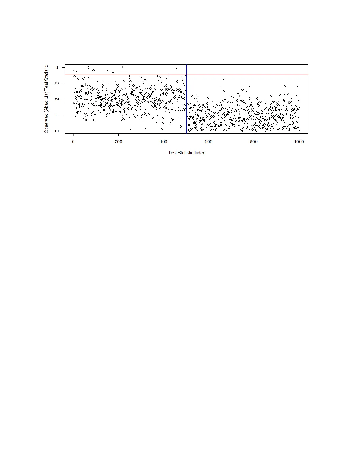
Impro ving the P o w er of Bonferroni Adjustmen ts under Join t Normalit y and Exc hangeabilit y Caleb Hil tunen and Yeonw oo Rho 1 Mic higan T ec hnological Univ ersity Abstract Bonferroni’s correction is a p opular to ol to address m ultiplicity but is notorious for its lo w p ow er when tests are dep enden t. This pap er proposes a practical mo dification of Bonferroni’s correction when test statistics are join tly normal and exc hangeable. This method is intuitiv e to practitioners and ac hieves higher pow er in sparse alternativ es, as our sim ulations suggest. W e also prov e that this method success- fully controls the family-wise error rate at any significance level. key wor ds : Bonferroni’s correction, Multiple comparisons, Exchangeable, Jointly normal test statistics. 1 In tro duction Multiple comparison correction pro cedures are b ecoming increasingly imp ortant with the prev alence of large datasets. When it comes to con trolling family-wise error rate (FWER), Bonferroni’s correction ( Bonferroni , 1936 ), for its ease of use, remains one of the popular methods among practitioners ( Polanin and Pigott , 2015 ), despite the existence of alternative approaches such as Tippett ( 1931 ); Fisher ( 1932 ); Pearson ( 1933 ); Osborn et al. ( 1949 ); Wilkinson ( 1951 ). Ho wev er, Bonferroni is also w ell-known for its conserv atism, particularly when the num b er of test statistics b ecomes v ery large or when tests are dep enden t ( Chen et al. , 2017 ). Curren tly , other metho ds exist whic h are not as conserv ativ e as Bonferroni in the face of dependence, such as Holm ( 1979 ), Benjamini and Ho ch b erg ( 1995 ), Proschan and Shaw ( 2011 ), Wilson ( 2019 ), and Liu and Xie ( 2020 ). In this pap er, we mo dify Bonferroni’s correction to improv e its p o wer under dep endence. W e limit our scop e to jointly normal test statistics that are inv ariant to p ermutations, i.e., exchangeable. W e also assume test statistics are standardized with v ariance 1. These assumptions are not to o uncommon in the p -v alue com bination literature ( Gupta et al. , 1973 ; Tian et al. , 2022 ; Choi and Kim , 2023 ; Gasparin et al. , 2025 ), as man y null distributions of test statistics are standard normal, and exchangeabilit y is the simplest assumption for dep endence when there are no sp ecific orders among the test statistics. By limiting its scop e, our metho d k eeps the in tuitiv e nature of Bonferroni’s and achiev es a significant impro vemen t in p ow er, particularly under sparse alternativ es, without assuming the kno wledge of any unknown parameters. 1 emails: C. Hiltunen (cahiltun@mtu.edu), Y. Rho (yrho@mtu.edu) 1 Our method is anc hored on Gupta et al. ( 1973 ), where a modification of Bonferroni’s is prop osed under join t normality and exchangeabilit y . How ever, their metho d requires information on the common pairwise correlation of ρ , which, in practice, is unknown. Estimation of ρ has b een somewhat dismissed in the p -v alue com bination literature, particularly when there is only one set of test statistics, p erhaps b ecause the absence of replication typically preven ts consisten t estimation via the w eak la w of large num bers. W e prop ose to estimate ρ using the sample v ariance. This is p ossible b ecause one set of p ositively correlated test statistics under the null w ould appear to b e clustered around a single random n umber. The magnitude of the correlation determines the tigh tness of the cluster, which can b e quantified by the sample v ariance. In fact, this idea is not entirely new. F ollmann and Prosc han ( 2013 ) proposed this estimator of ρ in a lo cation test with joint normal data with exc hangeabilit y . They developed a likelihoo d ratio test in this setting, demonstrating a use as O’Brien’s test ( O’Brien , 1984 ). Ho wev er, F ollmann and Proschan ( 2013 )’s approac h has received little atten tion in the p-v alue combination literature, and the idea of estimating ρ via sample v ariance has not b een applied to Gupta et al. ( 1973 )’s method. This pap er show cases the use of ρ estimation with Gupta et al. ( 1973 )’s mo dification of Bonferroni’s correction. This metho d b oasts higher p ow er under sparse alternatives, compared to the O’Brien’s test in F ollmann and Proschan ( 2013 ). It can also b e a practical alternative to recen tly developed p -v alue com bination metho ds based on hea vy-tails ( Wilson , 2019 ; Liu and Xie , 2020 ) when larger significance level is desired. As a Bonferroni-type pro cedure, our metho d allo ws easier identification of individual significan t tests following rejection of the global null, compared to the sum-based tests such as O’Brien’s and Wilson ( 2019 ); Liu and Xie ( 2020 ). This pap er is organized as follows. Section 2 introduces our metho d along with the theorems that prov e its v alidit y , and Section 3 explores the p erformance in finite samples. Section 4 provides concluding remarks. Pro ofs are relegated to App endix A . Appendix B presents size tables. 2 Metho d Let X = ( X 1 , ..., X n ) b e a sequence of jointly normal, exchangeable, and standardized test statistics with mean µ ∈ R n and p ositiv e semi-definite cov ariance matrix Σ ρ ∈ R n × R n , where ρ ∈ [0 , 1) indicates the common correlation. Consider the follo wing h yp othesis test, H 0 : µ = 0 H a : µ  = 0 , 2 where 0 is the zero vector of size n . While Gupta et al. ( 1973 ) dev elop their method for one-sided alternativ es, w e extend this framework to accommo date tw o-sided tests. F or brevity , we fo cus our description and sim ulations on the t wo-sided case, as the pro cedures for one-sided tests are similar. W e pro vide Theorem 2 detailing ho w our metho d can b e adapted for one-sided alternativ es. When normal v ariables are exchangeable, they can be expressed as X i = √ ρZ 0 + p 1 − ρZ i i = 1 , 2 , ..., n, where Z i are i.i.d v ariates pulled from standard normal distributions for i = 0 , 1 , ..., n . With this represen- tation, we will t weak the metho d describ ed in Gupta et al. ( 1973 ) for a tw o-sided alternative using similar metho ds found in Dunnett and Sob el ( 1955 ). W e combine our test statistics into a global test statistic, M n ( | X | ) = max 1 ≤ i ≤ n ( | X i | ), like in the Bonferroni case. W e aim for an exact 2 con trol of the FWER at some lev el α , so we would then find the critical v alue c α suc h that P ( M n ( | X | ) ≤ c α ) = P  max i     √ ρZ + p 1 − ρZ i     ≤ c α  = E Z h P  max i     √ ρZ + p 1 − ρZ i     ≤ c α | Z = z i = Z ∞ −∞ Ψ n µ = √ ρz ,σ = √ 1 − ρ ( c α ) ϕ ( z ) dz = 1 − α, where Ψ µ,σ ( · ) indicates the folded-normal distribution with an underlying normal v ariable of mean µ and standard deviation σ , and ϕ ( · ) indicates the standard normal densit y function. Here, we can then obtain the critical v alue c α through numerical integration. The global null H 0 is rejected when M n ( | X | ) ≥ c α . Alternativ ely , the p -v alue, p 0 , for this global test statistic, M n ( | X | ), can be calculated: the global null is rejected when p 0 ≤ α , where p 0 ( ρ ) = 1 − Z ∞ −∞ Ψ n µ = √ ρz ,σ = √ 1 − ρ ( M n ( | X | )) ϕ ( z ) dz . (GNP*) Gupta et al. ( 1973 ) provides a table of critical v alues c α for the one-sided alternative, assuming ρ is kno wn. Ho wev er, in practice, ρ is often unknown, making it imp ossible to use Gupta et al. ( 1973 )’s table. In this pap er, we propose to estimate ρ using F ollmann and Proschan ( 2013 )’s metho d-of-momen ts style estimator 3 : b ρ M OM = (1 − s 2 n ) I ( s 2 n < 1) . (MOM) 2 Exact control meaning that FWER = α as opp osed to strict control meaning FWER ≤ α . 3 It should b e noted that F ollmann and Proschan ( 2013 ) define their estimator as b ρ = max(0 , 1 − s 2 n ), which is equiv alent to MOM . As our framework was developed prior to our aw areness of F ollmann and Proschan ( 2013 ), we keep MOM in this form to ensure consistency with our theorems and pro ofs. 3 Here, s 2 n indicates the sample v ariance of X , s 2 n = 1 n − 1 X ′  I n − 1 n J n  X, where I n is identit y matrix of size n and J n is the matrix of ones of size n . While F ollmann and Prosc han ( 2013 ) also pro vide a maxim um-lik eliho o d estimator (MLE) of ρ , this paper will only consider MOM , since the tw o estimators are asymptotically equiv alent, as F ollmann and Proschan ( 2013 ) point out. While GNP* - MOM require n → ∞ , our simulation suggest that n = 20 is a go o d b enc hmark for arbitrary α and ρ such that α is con trolled. See T able 1 in App endix B . W e shall prov e that GNP* - MOM controls FWER. In fact, any other estimator of ρ that satisfies As- sumption 1 will w ork with GNP* . Assumption 1. p 2 ln( n )  √ 1 − ρ − p 1 − b ρ  P − − − − → n →∞ 0 . Theorem 1 prov es that b ρ M OM satisfies Assumption 1 . Theorem 1. Consider a se quenc e of jointly standar d normal r andom variables X = ( X 1 , ..., X n ) ′ wher e E [ X i ] = 0 , E [ X 2 i ] = 1 , C orr ( X i , X j ) = ρ for 1 ≤ i ≤ n, 1 ≤ j ≤ n, i  = j, and 0 < ρ < 1 . Then, with b ρ define d as in MOM , we have √ a n  p 1 − ρ − p 1 − b ρ  P − − − − → n →∞ 0 , wher e a n = o ( n ) . Since ln( n ) = o ( n ), Theorem 1 implies that MOM satisfies Assumption 1 . Theorem 2 prov es that GNP* - MOM con trols the FWER. Theorem 2. Consider a se quenc e of jointly standar d normal r andom variables X = ( X 1 , ..., X n ) ′ wher e E [ X i ] = 0 , E [ X 2 i ] = 1 , C orr ( X i , X j ) = ρ for 1 ≤ i ≤ n, 1 ≤ j ≤ n, i  = j, and 0 < ρ < 1 . Then, with M n ( X ) = max( X 1 , ..., X n ) , | X | = ( | X 1 | , ..., | X n | ) ′ , and and an estimator b ρ that satisfies Assumption 1 ,     Z ∞ −∞  Ψ n µ = √ ρz ,σ = √ 1 − ρ ( M n ( | X | )) − Ψ n µ = √ b ρz ,σ = √ 1 − b ρ ( M n ( | X | ))  ϕ ( z ) dz     P − − − − → n →∞ 0 , 4 wher e Ψ µ,σ ( · ) is the cumulative distribution function of the folde d-normal distribution with lo c ation µ and sc ale σ and ϕ ( · ) is the standar d normal density function. Conse quently, p 0 ( ρ ) − p 0 ( b ρ ) P − − − − → n →∞ 0 , wher e p 0 ( · ) is define d in GNP* . Because the observed p -v alue, p 0 ( b ρ ), conv erges to the theoretical p -v alue, p 0 ( ρ ), FWER is controlled. F or completeness, Theorem 3 pro v es FWER is con trolled in the one-sided test case. Without loss of generality , w e assume a p ositiv e alternativ e, H a : µ > 0 in this Theorem. F or negative alternativ e, H a : µ < 0, simply replace M n ( X ) with M n ( − X ). Theorem 3. Consider a se quenc e of jointly standar d normal r andom variables X = ( X 1 , ..., X n ) ′ wher e E [ X i ] = 0 , E [ X 2 i ] = 1 , C or r ( X i , X j ) = ρ for 1 ≤ i ≤ n, 1 ≤ j ≤ n, i  = j, and 0 < ρ < 1 . Then, with M n = max( X 1 , ..., X n ) and an estimator b ρ that satisfies Assumption 1 ,      Z ∞ −∞ Φ n  x √ ρ + M n ( X ) √ 1 − ρ  − Φ n x p b ρ + M n ( X ) p 1 − b ρ !! ϕ ( x ) dx      P − − − − → n →∞ 0 , implying c onver genc e of the p -value for M n ( X ) . Once the global null is rejected, this Bonferroni-type procedure allo ws an iden tification of significan t tests. A test statistic X i will b e significant if and only if X i ≥ c α , where c α can b e found through numerical in tegration. This metho d will alw ays yield the maximum, M n ( | X | ), as a signficant test statistic, though ma y b e to o conserv ativ e for the other test statistics. See Figure 3 for simulation evidence of the conserv ative nature and Section 4 for discussion on potential adjustments. 3 Sim ulation Studies When sim ulating the exchangeable sequence X , w e use the following computationally efficien t scheme, X i = √ ρZ 0 + p 1 − ρZ i + µ i , where Z i are indep endent and identically distributed standard normal v ariates for 0 ≤ i ≤ n . W e will p erform three sets of sim ulations. In the first tw o sets of simulations, the p o wer of GNP* - MOM (GNPMOM) 5 is compared against Bonferroni ( Bonferroni , 1936 ), HMP and HMP ADJ ( Wilson , 2019 ), and F-P ( Wilson , 2019 ). HMP indicates the harmonic mean of p -v alues, whereas HMP ADJ indicates the adjusted harmonic mean of p -v alues using the Landau distribution. The first set of simulations considers an extremely sparse alternative: µ = ( µ 1 , 0 , . . . , 0) ′ . µ 1 will b e selected from the range [0 , 3], increasing by 0.05 eac h run. W e set the num b er of iterations m = 10 , 000; n umber of test statistics n = 1 , 000; v arying ρ ∈ (0 . 0 , 0 . 2 , 0 . 5 , 0 . 9); and v arying FWER α ∈ (0 . 01 , 0 . 05 , 0 . 10). See results in Figure 1 . Observe that GNP* - MOM yields at least equal pow er compared to other methods. When ρ and α increase we are rewarded with increased p ow er while other metho ds falter. The second set of simulations considers an alternative which begins sparse and becomes more dense. In µ , the first n − s v alues are set to 0 while the other n − s + 1 v alues are set to p ln( n ) /s 0 . 1 , where s ∈ [0 , 1]. The same parameters m, n, ρ, α listed the paragraph abov e w ere used. F or results, refer to Figure 2 . When the ratio of non-zero means is less than 10%, GNP* - MOM app ears to attain higher p ow er compared to the other methods. This effect is particularly noticeable for larger ρ and α . The last sim ulation considers a µ where n/ 2 te st statistics attain mean 3 while the remaining n/ 2 test statistics attain mean 0. In this metho d, we set m = 1; n = 1 , 000; α = 0 . 10; and ρ = 0 . 5. The test statistics and plotted and a horizontal red line is imp osed to denote the critical v alue c α . See the results in Figure 3 . Although it is guaran teed to select the maxim um X ( n ) as a significan t test statistic, c α struggles to capture other test statistics which exist in the alternativ e h yp othesis. Out of 500 possible test statistics to capture, only 8 are denoted significan t. F urther refinemen t of this pro cess is discussed in Section 4 . Lastly , for size analysis of the metho ds, refer to App endix B . In the tables, we see that method GNP* - MOM provides exact con trol of α for v arying n , ρ , and α , while other metho ds do not pro vide exact con trol ev erywhere. 4 Conclusion In this pap er, we extended the one-sided findings presented in Gupta et al. ( 1973 ) to the t w o sided case and pro vided an implementable form using an estimator describ ed in F ollmann and Proschan ( 2013 ). This metho d pro vides a stable con trol of the FWER at size α as n → ∞ , with reasonable control already at n = 20. This metho d is intuitiv e as a Bonferroni-lik e pro cedure which is fav orable for practitioners. Ho wev er, numerical in tegration may b e a barrier for man y p eople. F or one-sided alternatives, refer to T able 1 in Gupta et al. ( 1973 ) after estimating ρ with MOM . The selection pro cess of significant test statistics can b e improv ed. Although guaranteed to yield the maxim um test statistic as significant, it fails to detect man y others. A couple of sequential-t yp e tests are 6 Figure 1: Comparison of the p ow er of GNP* against v arious metho ds when a single test statistic attains a non-zero mean. Size is indicated b y the horizontal black line. Note the higher p ow er achiev ed b y GNP* compared to the other methods. recommended for further inv estigation. One metho d in volv es directly using the distribution functions for the r th largest v ariates as describ ed in Gupta et al. ( 1973 ). The other metho d remov es the maximal data p oin t and reexamining the global hypothesis, repeating until a non-significant test app ears. One could also directly find the joint distribution of order statistics X (1) , ..., X ( n ) to solve for a critical v alue c α . F urther extensions in to the T case is desired, particularly the case of T statistics with differen t realized (indep enden t) χ 2 v ariates. 7 Figure 2: Comparison of the p ow er of GNP* against v arious metho ds as the proportion of test statistics attaining non-zero mean increases. Size is indicated by the horizontal black line. Note the higher p o wer ac hieved b y GNP* compared to the other metho ds when the prop ortion of non-zero mean test statistics is less than 10%. References Benjamini, Y. and Y. Ho ch berg (1995). Con trolling the false discov ery rate: A practical and p o werful approac h to m ultiple testing. Journal of the R oyal Statistic al So ciety: Series B 57 , 289–300. Bibinger, M. (2021). Gumbel con vergence of the maxim um of conv oluted half-normally distributed random v ariables. arXiv pr eprint arXiv:2103.14525 . Bishop, Y. M., S. E. F einberg, and P . W. Holland (1975, 2007). Discr ete Multivariate Analysis . Springer. Bonferroni, C. (1936). T eoria statistica delle classi e calcolo delle probabilita. Pubblic azioni del R istituto sup erior e di scienze e c onomiche e c ommericiali di fir enze 8 , 3–62. Chen, S.-Y., Z. F eng, and X. Yi (June 2017). A general in tro duction to adjustmen t for m ultiple comparisons. Journal of Thor acic Dise ase 9 (6), 1725–1729. Choi, W. and I. Kim (March 2023). Averaging p -v alues under exc hangeability . Statistics & Pr ob ability L etters 194 . 8 Figure 3: Absolute test statistics plotted based on index, where indices less than 500 attain mean 3 while others attain mean 0. The red line indicates the critical v alue while the blue line indicates the separation b et ween mean 3 and mean 0. Note the conserv ative nature of the critical v alue when detecting other test statistics whic h are not the maxim um. Dunnett, C. W. and M. Sobel (June 1955). Approximations to the probability integral and certain percentage p oin ts of a multiv ariate analogue of student’s t-distribution. Biometrika 42 (1/2), 258–260. Fisher, R. (1932). A Statistic al Metho d for R ese ar ch Workers (4th ed.). London: Oliv er and Bo yd. F ollmann, D. and M. Proschan (F ebruary 2013). A test of lo cation for exchangeable multiv ariate normal data with unknown correlation. Journal of Multivariate Analysis 104 (1), 115–125. Gasparin, M., R. W ang, and A. Ramdas (March 2025). Combining exchangeable p -v alues. Pr o c e e dings of the National A c adamy of Scienc es 122 (11), e2410849122. Gupta, S. S., K. Nagel, and S. Panc hapak esan (August 1973). On the order statistics from equally correlated normal random v ariables. Biometrika 60 (2), 403–413. Holm, S. (1979). A simple sequentially rejective multiple test pro cedure. Sc andinavian Journal of Statis- tics 6 (2), 65–70. Liu, Y. and J. Xie (2020). Cauc hy com bination test: A p ow erful test with analytic p -v alue calculation under arbitrary dependency structures. Journal of the Americ an Statistic al Asso ciation 115 (529), 393–402. Mukhopadh ya y , N. (2020). Pr ob ability and Statistic al Infer enc e . Routledge. O’Brien, P . C. (1984). Pro cedures for comparing samples with multiple endp oints. Biometrics , 1079–1087. 9 Osb orn, F., L. S. C. Jr., L. C. Devinney , C. I. Hovland, J. M. Russell, S. A. Stouffer, and D. Y oung (1949). Studies in So cial Psycholo gy in World War II , V olume I. Princeton Univ ersity Press. P earson, K. (1933). On a metho d of determining whether a sample of size n supp osed to ha ve been drawn from a parent p opulation having a kno wn probability integral has b een drawn at random. Biometrika 25 , 379–410. P olanin, J. R. and T. D. Pigott (Marc h 2015). The use of meta-analytic statistical significance testing. R ese ar ch Synthesis Metho ds 6 , 63–73. Prosc han, M. A. and P . A. Shaw (2011). Asymptotics of b onferroni for dependent normal test statistics. Statistics & Pr ob ability L etters 81 (7), 739–748. Tian, J., X. Chen, E. Katsevich, J. Go eman, and A. Ramdas (June 2022). Large-scale sim ulations inference under dependence. Sc andinavian Journal of Statistics 50 , 750–796. Tipp ett, L. (1931). Metho ds of Statistics . Williams Norgate. Wilkinson, B. (1951). A statistical consideration in psyc hological researc h. Psycholo gic al bul letin 48 , 156–158. Wilson, D. J. (Jan urary 2019). The harmonic mean p -v alue for com bining dep enden t tests. Pr o c. Natl. Avad. Sci. U.S.A. 116 (4), 1195–1200. 10 A Pro ofs Lemma 1. Consider a se quenc e of jointly standar d normal r andom variables X = ( X 1 , ..., X n ) ′ wher e E [ X i ] = 0 , E [ X 2 i ] = 1 , C or r ( X i , X j ) = ρ for 1 ≤ i ≤ n, 1 ≤ j ≤ n, i  = j, and 0 < ρ < 1 . Using the estimator c ρ a = 1 − s 2 n , wher e s 2 n indic ates the (unbiase d) sample varianc e, we have that c ρ a P − − − − → n →∞ ρ and c ρ a − ρ = O P  1 √ n  . Pr o of of L emma 1 . First, w e w ant to sho w that 1 − s 2 n P − − − − → n →∞ ρ. The sample v ariance is defined to be s 2 n = X ′  I n − 1 n J n  X n − 1 , where I n is the identit y matrix of size n and J n is the matrix of 1s of size n . So the expected v alue is E [ s 2 n ] = tr  I − 1 n J  n − 1 Σ ! = 1 − ρ, (1) where Σ is the matrix represen tation of the exc hangeable structure and tr( · ) is the trace of a matrix. Note then that ( n − 1) s 2 n 1 − ρ ∼ χ 2 ( n − 1) 11 so w e ha v e that V ar  ( n − 1) s 2 n 1 − ρ  = 2( n − 1) ⇒ V ar ( s 2 n ) = 2(1 − ρ ) 2 ( n − 1) . (2) So b y Cheb yshev’s, w e then hav e that ∀ ϵ > 0 , P ( | 1 − s 2 n − ρ | ≥ ϵ ) ≤ 2(1 − ρ ) 2 ( n − 1) ϵ 2 − − − − → n →∞ 0 , (3) whic h sufficien tly sho ws c ρ a P − − − − → n →∞ ρ . T o sho w c ρ a − ρ = O P  1 √ n  , w e apply Theorem 14.4-1 in Bishop et al. ( 2007 ), so c ρ a − ρ = O P  p V ar ( c ρ a )  = O P  1 √ n  . (4) Lemma 2. Consider the se quenc e of jointly standar d normal r andom variables define d in L emma 1. If we let I ( · ) r epr esent the indic ator function, we have then I ( s 2 n < 1) P − − − − → n →∞ 1 which, c onse quently, pr ovides us that 1. I ( s 2 n > 1) P − − − − → n →∞ 0 , 2. a n I ( s 2 n > 1) P − − − − → n →∞ 0 wher e a n ∈ R n . Pr o of of L emma 2 . W e w ant to sho w that I ( s 2 n < 1) P − − − − → n →∞ 1 whic h is equiv alent to the statemen t P ( s 2 n < 1) − − − − → n →∞ 1 . Recall that from Lemma 1 that w e can adjust s 2 n in to a χ 2 v ariable. Then, we can use the conv ergence 12 prop ert y from Chapter 5 of Mukhopadhy ay ( 2020 ) to sho w that P  ( n − 1) s 2 n 1 − ρ < n − 1 1 − ρ  = P   ( n − 1) s 2 n 1 − ρ − ( n − 1) p 2( n − 1) < n − 1 1 − ρ − ( n − 1) p 2( n − 1)   D − − − − → n →∞ P ( Z < ∞ ) = 1 (5) where Z ∼ N (0 , 1). Therefore, we hav e that I ( s 2 n < 1) P − − − − → n →∞ 1. Then consequence 1) is straigh tforw ard. F or consequence 2), we hav e then P  √ a n   I ( s 2 n > 1)   > ϵ  = P  I ( s 2 n > 1) > ϵ √ a n  =            0 if I ( s 2 n > 1) = 0 P ( s 2 n > 1) if I ( s 2 n > 1) = 1 (6) whic h, from consequence 1), pro duces conv ergence to 0 in probabilit y . Lemma 3. Consider the se quenc e of jointly standar d normal r andom variables define d in L emma 1 . Then, we have that b ρ = (1 − s 2 n ) I ( s 2 n < 1) P − − − − → n →∞ ρ Pr o of of L emma 3 . This is an application of Slutsky’s theorem with Lemma 1 and Lemma 2 . Pr o of of The or em 1 . Using T a ylor Series on f ( x ) = √ x cen tered at 1 − ρ , observe that f (1 − b ρ ) = p 1 − ρ + 1 2 √ 1 − ρ ( ρ − b ρ ) + R m ⇒ p 1 − b ρ − p 1 − ρ = 1 2 √ 1 − ρ ( ρ − b ρ ) + R m (7) where R m = P ∞ m =2 f ( m ) (1 − ρ )( ρ − b ρ ) m m ! ∼ O P (( p − b ρ ) m ) = O p  1 √ n  m  . So to show that Ass umption 1 holds 13 for b ρ , we simply ha ve to sho w that √ a n ( ρ − b ρ ) P − − − − → n →∞ 0. With c ρ a = 1 − s 2 n as in Lemma 1 , w e ha v e that √ a n ( b ρ − ρ ) = √ a n  (1 − s 2 n ) I ( s 2 n < 1) − ρ − ρI ( s 2 n < 1) + ρI ( s 2 n < 1  = √ a n ( c ρ a − ρ ) I ( s 2 n < 1) − √ a n I ( s 2 n > 1) ρ = o  √ n  O p  1 √ n  I ( s 2 n < 1) − o  √ n  I ( s 2 n > 1) ρ. (8) Here, b oth o ( √ n ) O p  1 √ n  I ( s 2 n < 1) and p ln( n ) I ( s 2 n > 1) ρ conv erges to 0 in probability through Slutsky’s theorem and Lemma 2 . Consequently , √ a n R m P − − − − → n →∞ 0 as well, so then b y the contin uous mapping theorem, the en tire expression conv erges to 0 in probabilit y and Assumption 1 holds. Pr o of of The or em 3 . First let F n ( x, ρ, M n ) = Φ n  x √ ρ + M n √ 1 − ρ  for brevit y , and see from the mean v alue theo- rem that we can find some c x suc h that     Z ∞ −∞ ( F ( x, ρ, M n ( X )) − F ( x, b ρ, M n ( X ))) ϕ ( x ) dx     ≤ Z ∞ −∞ | ( F ( x, ρ, M n ( X )) − F ( x, b ρ, M n ( X ))) ϕ ( x ) | dx = Z ∞ −∞ n (Φ( c x )) n − 1 ϕ ( c x )      x √ ρ + M n ( X ) √ 1 − ρ − x p b ρ + M n ( X ) p 1 − b ρ      ϕ ( x ) dx ≤ 1 √ 2 π Z ∞ −∞ n Φ n − 1 ( c x ) | f n ( x, ˆ ρ, ρ ) | ϕ ( x ) dx where f n ( x, b ρ, ρ ) = 1 √ 1 − ρ p 1 − b ρ · ( A n ( ρ ) p 1 − b ρ − A n ( ρ ) p 1 − ρ ) − p 2 ln( n )(1 − ρ )( p 1 − ρ − p 1 − b ρ ) + x ( √ ρ p 1 − b ρ − p b ρ p 1 − ρ ) and observ e that n Φ n − 1 ( c x ) − − − − → n →∞ 0 since Φ( c x ) ∈ (0 , 1). Then, we hav e f n ( x, b ρ, ρ ) D − − − − → n →∞ 0 p oin twise in x through the con tinuous mapping theorem and the assumption. Because F ( x, ρ, M n ( X )) − F ( x, b ρ, M n ( X )) − − − − → n →∞ 0 14 p oin twise in x and is dominated by ϕ ( x ), we hav e b y the dominated conv ergence theorem that lim n →∞ Z ∞ −∞ n Φ n − 1 ( c x ) | f n ( x, ˆ ρ, ρ ) | ϕ ( x ) dx = Z ∞ −∞ lim n →∞ n Φ n − 1 ( c x ) | f n ( x, ˆ ρ, ρ ) | ϕ ( x ) dx = 0 whic h concludes the pro of. Lemma 4. Consider a se quenc e of jointly standar d normal r andom variables define d in The or em 2 and define M n ( X ) = max( X 1 , ..., X n ) . Then, we have that P ( M n ( | X | ) > c α ) = 1 − Z ∞ −∞ Ψ n µ = √ ρz ,σ = √ 1 − ρ ( c α ) ϕ ( z ) dz wher e ϕ ( · ) is the standar d normal density function, Ψ µ,σ ( · ) is the cumulative distribution function of | Y | when Y ∼ N ( µ, σ ) , and c α is some r e al numb er. Pr o of of L emma 4 . Since X 1 , ..., X n are N (0 , 1) with equicorrelation ρ , w e are able to express these X i as X i = √ ρZ + p 1 − ρZ i , where Z and Z i are N (0 , 1) and all are join tly independent. Then, we hav e that P ( M n ( | X | ) > c α ) = 1 − P ( M n ( | X | ) < c α ) = 1 − P  M n     √ ρZ + p 1 − ρZ i     < c α  = 1 − E Z h P  M n     √ ρZ + p 1 − ρZ i     < c α | Z = z i = 1 − Z ∞ −∞ P  M n     √ ρz + p 1 − ρZ i     < c α  ϕ ( z ) dz . (9) Here, since Z = z is giv en, w e ha ve √ ρz + √ 1 − ρZ i ∼ N ( √ ρz , √ 1 − ρ ) and they are i.i.d . W e then hav e ( 9 ) = 1 − Z ∞ ∞ P ( M n ( | √ ρz + p 1 − ρZ 1 | ) < c α ) n ϕ ( z ) dz = 1 − Z ∞ −∞ Ψ n µ = √ ρz ,σ = √ 1 − ρ ( c α ) ϕ ( z ) dz . Pr o of of The or em 2 . The cum ulative distribution function for the folded normal distribution follo ws Ψ µ,σ ( x ) = 1 2  erf  x + µ σ √ 2  + erf  x − µ σ √ 2  , 15 where erf( · ) is the error function, erf( x ) = 2 √ π Z x 0 e − t 2 dt, so w e can show through t wo consecutive applications of the mean v alue theorem that ( 2 ) ≤ Z ∞ −∞      c n − 1 z , 1 n 2 n 2 e − c 2 z, 2 √ π g 1 ( z , ρ, b ρ ) + 2 e − c 2 z, 3 √ π g 2 ( z , ρ, b ρ ) ! ϕ ( z )      dz , (10) where c z 1 ∈ ( − 2 , 2) since erf( x ) ∈ ( − 1 , 1) for all x , c z 2 and c z 3 are in R dep enden t on z , and g 1 ( z , ρ, b ρ ) = M n ( | X | ) + √ ρz √ 1 − ρ − M n ( | X | ) + p b ρz p 1 − b ρ , g 2 ( z , ρ, b ρ ) = M n ( | X | ) − √ ρz √ 1 − ρ − M n ( | X | ) − p b ρz p 1 − b ρ . Note that since c z 1 ∈ ( − 2 , 2), then c n − 1 z 1 n 2 n − − − − → n →∞ 0. Then, for g 1 , w e ha v e that p (1 − ρ )(1 − b ρ ) g 1 ( z , ρ, b ρ ) = M n ( | X | )  p 1 − ρ − p 1 − b ρ  + z  √ ρ p 1 − b ρ − p b ρ p 1 − ρ  . (11) Note that M n ( | X | ) = max i     √ ρz + p 1 − ρZ i     ≤ √ ρ | z | + p 1 − ρ max i ( | Z i | ) . F rom Bibinger ( 2021 ), w e ha ve that a n (max i ( | Z i | − b n ) D − − − − → n →∞ G, where a n = 1 p 2 ln(2 n ) , b n = p 2 ln(2 n ) − ln(4 π ln(2 n )) 2 p 2 ln(2 n ) , and G is the standard Gumbel distribution. Then, M n ( | X | )  p 1 − ρ − p 1 − b ρ  ≤  √ ρ | z | + p 1 − ρ  a n  max i | Z i | − b n  1 a n + a n b n   p 1 − ρ − p 1 − b ρ  , where then note that p 1 − ρ − p 1 − b ρ P − − − − → n →∞ 0 , 1 a n = o ( √ n ) ⇒ 1 a n  p 1 − ρ − p 1 − b ρ  P − − − − → n →∞ 0 , 16 a n b n − − − − → n →∞ 1 , and a n  max i ( | Z i | ) − b n   p 1 − ρ − p 1 − b ρ  D − − − − → n →∞ 0 . Through the contin uous mapping theorem and similar arguments for g 2 , see that ( 11 ) D − − − − → n →∞ 0 p oin twise in z . Then, follo wing the same final steps from Theorem 2 , we hav e our conclusion. B Size tables 17 Empirical Size for ρ = 0 . 0 α = 0 . 01 α = 0 . 05 α = 0 . 10 Metho d n =20 n =100 n =1000 n =20 n =100 n =1000 n =20 n =100 n =1000 GNPMLE 0.0103 0.0099 0.0105 0.0524 0.0492 0.0470 0.1045 0.0967 0.0997 HMP 0.0107 0.0109 0.0115 0.0711 0.0751 0.00895 0.1753 0.2230 0.3619 HMP ADJ 0.0103 0.0100 0.0104 0.0518 0.0481 0.0499 0.1008 0.0951 0.0983 Bonferroni 0.0103 0.0099 0.0104 0.0506 0.0474 0.0455 0.0989 0.0917 0.0952 F-P 0.0037 0.0044 0.0042 0.0234 0.0227 0.0233 0.0496 0.0519 0.0474 Empirical Size for ρ = 0 . 2 α = 0 . 01 α = 0 . 05 α = 0 . 10 Metho d n =20 n =100 n =1000 n =20 n =100 n =1000 n =20 n =100 n =1000 GNPMLE 0.0090 0.0081 0.0102 0.0504 0.0504 0.0507 0.1011 0.0965 0.0917 HMP 0.0106 0.0105 0.0144 0.0716 0.0860 0.1151 0.1647 0.2064 0.2753 HMP ADJ 0.0100 0.0091 0.0127 0.0528 0.0589 0.0689 0.1031 0.1049 0.1159 Bonferroni 0.0089 0.0078 0.0093 0.0476 0.0460 0.0439 0.0920 0.0831 0.0707 F-P 0.0639 0.0593 0.0101 0.1241 0.1111 0.0532 0.1681 0.1586 0.1064 Empirical Size for ρ = 0 . 5 α = 0 . 01 α = 0 . 05 α = 0 . 10 Metho d n =20 n =100 n =1000 n =20 n =100 n =1000 n =20 n =100 n =1000 GNPMLE 0.0091 0.0099 0.0112 0.0460 0.0524 0.0481 0.1004 0.0941 0.1000 HMP 0.0130 0.0143 0.0172 0.0671 0.0830 0.0844 0.1471 0.1609 0.1764 HMP ADJ 0.0120 0.0133 0.0150 0.0511 0.0607 0.0555 0.0993 0.0931 0.0905 Bonferroni 0.0080 0.0070 0.0057 0.0347 0.0291 0.0194 0.0690 0.0471 0.0314 F-P 0.0219 0.0124 0.0102 0.0639 0.0570 0.0493 0.1182 0.0993 0.1010 Empirical Size for ρ = 0 . 9 α = 0 . 01 α = 0 . 05 α = 0 . 10 Metho d n =20 n =100 n =1000 n =20 n =100 n =1000 n =20 n =100 n =1000 GNPMLE 0.0112 0.0095 0.0095 0.0479 0.0502 0.0486 0.0990 0.0977 0.1067 HMP 0.0119 0.0105 0.0110 0.0523 0.0554 0.0529 0.1070 0.1073 0.1152 HMP ADJ 0.0112 0.0098 0.0093 0.0388 0.0408 0.0363 0.0745 0.0652 0.0601 Bonferroni 0.0033 0.0014 0.0005 0.0106 0.0047 0.0008 0.0215 0.0080 0.0022 F-P 0.0108 0.0096 0.0094 0.0467 0.0523 0.0486 0.1009 0.0974 0.1051 T able 1: Empirical size for v arying ρ , α , and n . Note that GNP* pro vides exact con trol of α for each possible com bination of parameters, whereas other methods falter in certain com binations. 18