Stochastic Gradient Variational Inference with Price's Gradient Estimator from Bures-Wasserstein to Parameter Space

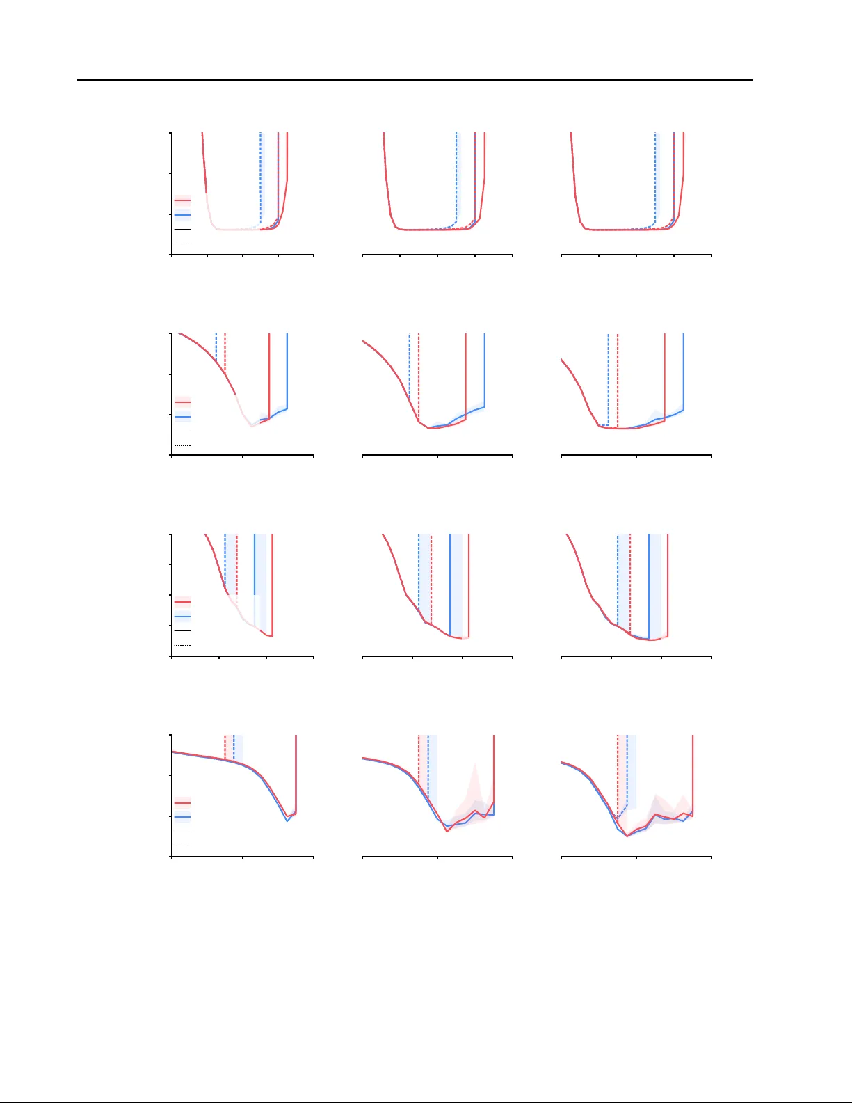
Stochastic Gradient V ariational Infer ence with Price’ s Gradient Estimator fr om Bur es-W asserstein to Parameter Space K yurae Kim 1 Qiang Fu 2 Y i-An Ma 3 Jacob R. Gardner 1 T revor Campbell 4 Abstract For approximating a target distribution gi ven only its unnormalized log-density , stochastic gradient- based variational inference (VI) algorithms are a popular approach. For e xample, W asserstein VI (WVI) and black-box VI (BBVI) perform gradi- ent descent in measure space (Bures-W asserstein space) and parameter space, respectively . Previ- ously , for the Gaussian variational family , con ver - gence guarantees for WVI hav e sho wn superiority ov er existing results for black-box VI with the reparametrization gradient, suggesting the mea- sure space approach might pro vide some unique benefits. In this work, howe ver , we close this gap by obtaining identical state-of-the-art itera- tion complexity guarantees for both. In particular , we identify that WVI’ s superiority stems from the specific gradient estimator it uses, which BBVI can also le verage with minor modifications. The estimator in question is usually associated with Price’ s theorem and utilizes second-order informa- tion (Hessians) of the target log-density . W e will refer to this as Price’ s gradient. On the flip side, WVI can be made more widely applicable by us- ing the reparametrization gradient, which require s only gradients of the log-density . W e empirically demonstrate that the use of Price’ s gradient is the major source of performance improv ement. 1. Introduction V ariational inference (VI; Jordan et al. , 1998 ; Blei et al. , 2017 ; Peterson & Hartman , 1989 ; Hinton & van Camp , 1993 ) is a collection of algorithms for approximating a target 1 Univ ersity of Pennsylvania, Philadelphia, U.S. 2 Y ale Univ er- sity , New Hav en, U.S. 3 Univ ersity of California San Diego, San Diego, U.S. 4 Univ ersity of British Columbia, V ancouver , Canada. Correspondence to: Kyurae Kim < kyrkim@seas.upenn.edu >, Qiang Fu < qiang.fu@yale.edu >, Y i-An Ma < yianma@ucsd.edu >, Jacob R. Gardner < jacobrg@seas.upenn.edu >, T revor Campbell < trev or@stat.ubc.ca >. Pr eprint. F ebruary 24, 2026. distribution π over some family of parametric distrib utions Q when only the unnormalized density of π , denoted by e π , is av ailable. When π is supported on R d such that its associated potential function U = − log e π is in R d → R , it is common to lev erage stochastic gradient-based algorithms, as they only require local information of U ( Grav es , 2011 ; Salimans & Knowles , 2013 ; Wingate & W eber , 2013 ; T itsias & Lázaro-Gredilla , 2014 ; Ranganath et al. , 2014 ; Kingma & W elling , 2014 ; Rezende et al. , 2014 ). Most VI algorithms are designed to minimize the variational free energy , also known as the negati ve e vidence lower bound ( Jordan et al. , 1999 ), defined as F ( q ) ≜ E ( q ) + H ( q ) , where E is the en- ergy functional associated with U , while H is the Boltzmann entropy . That is, we solve minimize q ∈Q  F ( q ) = KL( q , π ) + F ( π )  through only zeroth-, first-, and second-order information of U . Since F is equal to the e xclusive KL div ergence ( Kull- back & Leibler , 1951 ) between q and π up to the constant F ( π ) , this also minimizes q 7→ KL( q , π ) . A common approach for minimizing F is, informally speak- ing, to lev erage some sort of stochastic gradient descent (SGD; Robbins & Monro , 1951 ; Bottou , 1999 ; Bottou et al. , 2018 ; Bach & Moulines , 2011 ; Nemirovski et al. , 2009 ; Shalev-Shw artz et al. , 2011 ) scheme, where intractable terms (such as the gradient of the energy E ) are stochas- tically estimated. There are two popular ways to realize this conceptual algorithm. The most widely used approach in practice is to represent each q λ ∈ Q via a Euclidean vector of variational parameter s λ ∈ Λ , and run gradient descent on the Euclidean space of parameters Λ ⊆ R p ( W ingate & W eber , 2013 ; Kucukelbir et al. , 2017 ; T itsias & Lázaro- Gredilla , 2014 ; Ranganath et al. , 2014 ; Salimans & Knowles , 2013 ). This is now referred to as blac k-box variational in- fer ence (BBVI). The other approach is to define a tractable notion of measure-v alued deriv atives, which can directly perform gradient descent in measure space. In particular, recent advances in our understanding of the W asserstein geometry ( V illani , 2009 ; Chewi et al. , 2025 ) and gradient flows ( Ambrosio et al. , 2005 ; Jordan et al. , 1998 ) ha ve con- tributed to the de velopment of (parametric 1 ) W asserstein 1 W e focus on WVI on par ametric families, which excludes 1 SGVI with Price’ s Gradient Estimator from Bures-W asserstein to Parameter Space T able 1. Overvie w of Main Theoretical Results. Algorithm Space Gradient Estimator Maximum Step Size Iterations Complexity Reference SPGD Λ Reparam. 1 / ( dLκ ) dκ 2 tr( µ Σ ∗ ) 1 / ϵ Domke et al. ( 2023 ) Kim et al. ( 2023 ) SPBWGD BW( R d ) Bonnet-Price 1 / ( Lκ 2 ) dκ 1 ϵ log 1 ϵ + κ 3 log  ∆ 2 1 ϵ  Diao et al. ( 2023 ) SPGD Λ Bonnet-Price 1 / ( Lκ ) dκ 1 ϵ + √ d κ 3 / 2 log  κ ∆ 2  1 √ ϵ + κ 2 log 1 ϵ Theorem 3.3 SPBWGD BW( R d ) Bonnet-Price 1 / ( Lκ ) dκ 1 ϵ + √ d κ 3 / 2 log  κ ∆ 2  1 √ ϵ + κ 2 log 1 ϵ Theorem 3.2 Note: The complexity statements assume µ -strong con vexity and L -smoothness of U (Assumption 3.1 ); ϵ > 0 is the target accurac y lev el for ensuring µ E W 2 ( q T , q ∗ ) 2 ≤ ϵ , where q T is the last iterate and q ∗ is the global minimizer of F ; κ = L/µ is the condition number; ∆ is the distance between the initialization and the optimum. vari ational inference (WVI; Lambert et al. , 2022 ; Diao et al. , 2023 ; Huix et al. , 2024 ; T alamon et al. , 2025 ) algorithms that take this route. W e also note that natural gradient VI algorithms ( Khan & Rue , 2023 ; Khan & Nielsen , 2018 ; Lin et al. , 2019 ; T an , 2025 ) utilize parameter gradients while measuring distance using the KL pseudo-metric. Howe ver , NGVI will not be the focus of this work. Giv en that the WVI methods utilize a proper metric ( V illani , 2009 ) between measures—the W asserstein-2 metric W 2 — it is natural to e xpect them to outperform BBVI. Indeed, current theoretical e vidence suggests that this is the case. Consider the Gaussian variational family , also known as the Bures-W asserstein space ( Bures , 1969 ; Bhatia et al. , 2019 ), set as Q = BW ( R d ) ≜ { Normal( m, Σ) | m ∈ R d , Σ ∈ S d ≻ 0 } . Here, (BW( R d ) , W 2 ) forms a metric space. Denot- ing the global minimizer as q ∗ = Normal( m ∗ , Σ ∗ ) = arg min q ∈Q F ( q ) , for a µ -strongly con vex and L -smooth potential U , the algorithm by Diao et al. ( 2023 ) re- quires O  dκϵ − 1 log ϵ − 1 + κ 3 log ϵ − 1  steps to ensure µ E [W 2 ( q , q ∗ ) 2 ] ≤ ϵ . In contrast, the BBVI equiv alent with a certain cov ariance parametrization, the reparametrization gradient estimator ( Ho & Cao , 1983 ; Rubinstein , 1992 ), and stochastic proximal gradient descent (SPGD; Nemirovski et al. , 2009 ) requires O  dκ 2 tr( µ Σ ∗ ) ϵ − 1  steps ( Kim et al. , 2023 ; Domke et al. , 2023 ). It might therefore appear that the guarantees for BBVI are weaker in the limit ϵ → 0 . In this work, we demonstrate that the dif ference in theoreti- cal guarantees originates from the specific gradient estimator for the scale parameter used in stochastic implementations of WVI rather than the geometry being used. The estimator in question can be derived via Price’ s theorem ( Price , 1958 ) and leverages second-order information (Hessians) of the tar- get log-density . W e will refer to this as Price’ s gradient esti- mator . Through Stein ( Liu , 1994 ; Stein , 1981 ) or Price’ s the- orem, BBVI with SPGD can also make use of essentially the same gradient estimator , resulting in an iteration comple x- particle-based WVI methods. ity of O  dκϵ − 1 + √ d κ 3 / 2 log  κ ∆ 2  ϵ − 1 / 2 + κ 2 log ϵ − 1  . Furthermore, to ensure a f air comparison, we present a re- fined analysis of the WVI counterpart of SPGD ( Diao et al. , 2023 ), resulting in an iteration complexity of O  dκϵ − 1 + √ d κ 3 / 2 log  κ ∆ 2  ϵ − 1 / 2 + κ 2 log ϵ − 1  . These results sug- gest that the specific implementation of BBVI studied here and WVI might not be that different after all. While this has been suggested by Y i & Liu ( 2023 ); Hoffman & Ma ( 2020 ), this work further supports this f act by contributing a non-asymptotic discrete-time analysis. Our theoretical results are organized in T able 1 . In addition, we demonstrate that WVI can also leverage the reparametrization gradient traditionally used in BBVI ( T it- sias & Lázaro-Gredilla , 2014 ; Kingma & W elling , 2014 ; Rezende et al. , 2014 ). Unlike Price’ s gradient previously used in WVI, the reparametrization gradient only requires first-order information ( ∇ U ). Thus, the resulting WVI algo- rithm should be more widely applicable in practice. Giv en this fact, we empirically compare the performance of BBVI and WVI, both with the Hessian-based gradient estimators and the reparametrization gradient. Results demonstrate that a large fraction of the performance difference stems from the use of Hessian-based gradients, supporting the claim that the gradient estimator is the main source of performance. 2. Background Notation. For any x, y ∈ R d , we denote the Euclidean inner product and norm as ⟨ x, y ⟩ = x ⊤ y and ∥ x ∥ 2 ≜ p ⟨ x, x ⟩ . For any matrix A, B ∈ R d × d , tr( A ) ≜ P d i =1 A ii , ⟨ A, B ⟩ F ≜ tr( A ⊤ B ) , ∥ A ∥ F ≜ p ⟨ A, A ⟩ F , and the ℓ 2 operator norm of A is denoted as ∥ A ∥ 2 . The symmetric and positive definite subsets of R d × d will be denoted as S d and S d ≻ 0 , while L d ≻ 0 denotes the set of lower -triangular matrices with strictly positi ve eigen val- ues. W e will represent a measure and its density with the same symbol. For the space of square-integrable mea- sures P 2 ( X ) ≜ { q | R X ∥ x ∥ 2 d q ( x ) < + ∞} , for some q ∈ P 2 ( R d ) , the set of inte grable functions is denoted as L 2 ( q ) ≜  f | R ∥ f ∥ 2 2 d q < + ∞  . For any two prob- 2 SGVI with Price’ s Gradient Estimator from Bures-W asserstein to Parameter Space ability measures p, q ∈ P 2  R d  , we denote the set of couplings between the two as Ψ( p, q ) . Then the squared W asserstein-2 distance between p and q is W 2 ( p, q ) 2 ≜ inf ψ ∈ Ψ( p,q ) R R d × R d ∥ x − y ∥ 2 2 d ψ ( x, y ) . For some measur- able map M : R d → R d and measure q supported on R d , M # q denotes the corresponding push-forward measure. Un- less stated otherwise, the coupling attaining the infimum of W 2 , ψ ∗ ∈ Ψ( p, q ) , is referred to as “the optimal coupling, ” which is guaranteed to exist ( V illani , 2009 , Theorem 4.1) and is unique by Brenier’ s Theorem ( Brenier , 1991 ). 2.1. Problem Setup Our focus will be on first-order stochastic optimization al- gorithms for solving the problem minimize q ∈Q n F ( q ) ≜ E ( q ) + H ( q ) o , where E ( q ) ≜ R R d U ( z ) q (d z ) (Energy) H ( q ) ≜ R R d log q ( z ) q (d z ) . (Boltzmann entropy) W e consider the “non-conjugate” setup, where E is in- tractable due to the expectation over q . Suppose we can parametrize each q λ ∈ Q with a Euclidean vector of param- eters λ ∈ Λ . Then it is equiv alent to minimize λ 7→ F ( q λ ) ov er the Euclidean parameter space Λ ⊆ R p . Informally speaking, when U is “regular , ” E also tends to be regular . For instance, if U is Lipschitz-smooth, then E also tends to exhibit appropriate notion of Lipschitz- smoothness ( Domke , 2020 ; Diao et al. , 2023 ; Lambert et al. , 2022 ). The entropy term H , howe ver , does not enjoy Lip- schitz smoothness in general. For instance, for Gaussians q = Normal( m, Σ) , H ( q ) blows up as the covariance Σ becomes singular . T ypically , in optimization, such non- smoothness is remedied by relying on proximal gradient algorithms ( Wright & Recht , 2021 , §9.3). Indeed, for min- imizing F , stochastic proximal gradient algorithms have been proposed for both the Bures-W asserstein ( Diao et al. , 2023 ) and Euclidean parameter spaces ( Domk e , 2020 ). In the following sections, we will introduce these algorithms. 2.2. W asserstein V ariational Infer ence via Stochastic Proximal Bur es-W asserstein Gradient Descent Since the seminal work of Jordan et al. ( 1998 ), it is kno wn that F can be minimized by simulating its W asserstein gra- dient flo w . The forward-backward discretization of this flo w results in the W asserstein-analog of proximal gradient de- scent ( W ibisono , 2018 ; Bernton , 2018 ; Salim et al. , 2020 ) operating on the metric space ( P 2 ( R d ) , W 2 ) . This algo- rithm, howe ver , is not directly implementable. Recently , Lambert et al. ( 2022 ); Diao et al. ( 2023 ) demonstrated that, by constraining optimization to the Bur es -W asserstein mani- fold BW( R d ) ⊂ P 2 ( R d ) ( Bures , 1969 ; Bhatia et al. , 2019 ), the algorithm becomes implementable. In particular, the proximal Bures-W asserstein gradient descent scheme iter- ates, for each t ≥ 0 , q t + 1 / 2 = (Id − γ t ∇ BW E ( q t )) # q t (1) q t +1 = JK O γ t H ( q t + 1 / 2 ) , where, for any q = Normal( m, Σ) ∈ BW  R d  , the Bures- W asserstein gradient of E can be deriv ed ( Lambert et al. , 2022 , Appendix C) as ∇ BW E ( q ) ≜ x 7→ ∇ m E ( q ) + 2 ∇ Σ E ( q )( x − m ) , while the W asserstein-analog of the proximal operator , com- monly referred to as the “JK O operator , ” is defined as, for any functional G : BW( R d ) → R ∪ { + ∞} satisfying some mild regularity conditions, JK O G ( q ) ≜ arg min p ∈ BW( R d ) n G ( p ) + ( 1 / 2 )W 2 ( p, q ) 2 o . For the Bures-W asserstein space, the proximal operator has a tractable closed-form expression ( W ibisono , 2018 , Exam- ple 7), which is key to implementing the algorithm. Still, the Bures-W asserstein gradient in volves e xpectations ov er q = Normal( µ, Σ) that are generally not tractable. Therefore, these hav e to be replaced with stochastic esti- mates ( Lambert et al. , 2022 ) of ∇ m E and ∇ Σ E resulting in an estimator of the Bures-W asserstein gradient [ ∇ BW E ( q ; ϵ ) ≜ x 7→ [ ∇ m E ( q ; ϵ ) + 2 [ ∇ Σ E ( q ; ϵ )( x − m ) , where ϵ ∼ φ = Normal(0 d , I d ) is standard Gaussian noise. Replacing ∇ BW E in Eq. ( 1 ) with [ ∇ BW E results in stochastic proximal Bures-W asserstein gradient descent (SPBWGD; Diao et al. , 2023 ). Lambert et al. ; Diao et al. rely on the estimators \ ∇ bonnet m E ( q ; ϵ ) ≜ ∇ U ( Z ) \ ∇ price Σ E ( q ; ϵ ) ≜ ( 1 / 2 ) ∇ 2 U ( Z ) , (2) where Z = cholesky(Σ) ϵ + µ . The fact that these estimators are unbiased follo ws from the theorems by Bonnet ( 1964 ) and Price ( 1958 ) or Riemannian geometry ( Altschuler et al. , 2021 , Appendix B.3). For each t ≥ 0 , the resulting update rule for the iterate q t = Normal( m t , Σ t ) is m t +1 = m t − γ t \ ∇ m t E ( q t ; ϵ t ) M t +1 = I d − 2 γ t \ ∇ Σ t E ( q t ; ϵ t ) Σ t + 1 / 2 = M t +1 Σ t M ⊤ t +1 Σ t +1 = 1 2  Σ t + 1 / 2 + 2 γ t I d +  Σ t + 1 / 2  Σ t + 1 / 2 + 4 γ t I d  1 / 2  , where the standard Gaussian noise sequence ( ϵ t ) t ≥ 0 is sam- pled as ϵ t i . i . d . ∼ φ . Note the update rule for Σ t +1 / 2 is dif fer- ent from the one originally presented by Diao et al. ( 2023 ); 3 SGVI with Price’ s Gradient Estimator from Bures-W asserstein to Parameter Space a transpose has been added to M t +1 . This change will be- come necessary later in Section 4 when we replace [ ∇ Σ E with an estimator that is not almost surely symmetric. 2.3. Black-Box V ariational Inference via Stochastic Proximal Gradient Descent An alternati ve to SBWPGD is to optimize over the Eu- clidean space of parameters Λ . Recall, in this case, each q λ ∈ Λ is assumed to be associated with a Euclidean vector λ ∈ Λ . Then, if we hav e access to an unbiased estimator of ∇ λ E ( q λ ) , denoted as d ∇ λ E ( q λ ) , F can be minimized via SPGD, which, for each t ≥ 0 , updates the variational parameters λ t as λ t + 1 / 2 = λ t − γ t [ ∇ λ t E ( q λ t ; ϵ t ) λ t +1 = pro x λ 7→ γ t H ( q λ )  λ t + 1 / 2  , where ϵ t i . i . d . ∼ φ is some randomness source and pro x is the canonical Euclidean proximal operator ( Parikh & Boyd , 2014 ) defined as, for any proper lower semi-continuous con vex function g : R p → R ∪ { + ∞} , pro x g ( λ ) ≜ arg min λ ′ ∈ Λ  g ( λ ′ ) + ( 1 / 2 ) ∥ λ ′ − λ ∥ 2 2  . For some classes of v ariational families Q and parametriza- tions, the proximal operator can be made tractable ( Domke , 2020 ). Before that, ho wever , we must come up with an unbiased estimator of the parameter gradient ∇ λ E ( q λ ) . Suppose the variational family Q and the parametrization λ 7→ q λ satisfy the following: Definition 2.1. F or some Λ ⊂ R p , the variational family Q = { q λ | λ ∈ Λ } is referr ed to as a r eparameterizable family if ther e exists some bijective map ϕ λ : R d → R d differ entiable with r espect to λ and a base distribution φ ∈ P 2 ( R d ) such that, for all λ ∈ Λ , Z ∼ q λ ⇔ Z d = ϕ λ ( ϵ ) ; ϵ ∼ φ . Here, d = is equi v alence in distrib ution. Then an immediate option for estimating ∇ λ E ( q λ ) is to use the reparametriza- tion gradient ( Ho & Cao , 1983 ; Rubinstein , 1992 ; see also Mohamed et al. , 2020 ) \ ∇ rep λ E ( q λ ) ≜ ∇ λ ϕ λ ( ϵ ) ∇ U ( ϕ λ ( ϵ )) , (3) which can be derived by combining the law of the un- conscious statistician with the Leibniz integral rule. This combination of SGD with the reparametrization gradient— commonly referred to as BBVI—is widely used in prac- tice through probabilistic programming frameworks such as Stan ( Carpenter et al. , 2017 ), T uring ( Fjelde et al. , 2025 ), Pyro ( Bingham et al. , 2019 ), and PyMC ( Patil et al. , 2010 ). The wide adoption of BBVI in practice is partly due to its flexibility: Definition 2.1 applies to a very wide range of families from Gaussians ( T itsias & Lázaro-Gredilla , 2014 ) to normalizing flo ws ( Rezende & Mohamed , 2015 ). Fur - thermore, Eq. ( 3 ) uses only gradients of U , which can be efficiently computed via automatic dif ferentiation ( Kucukel- bir et al. , 2017 ). In this work, howe ver , we will further restrict our attention to the Gaussian variational family with a specific parametrization: Assumption 2.2. The variational family Q is the Gaus- sian variational family , wher e each member q λ = Normal( m, C C ⊤ ) ∈ Q is parametrized as Λ =  λ = ( m, vec( C )) | m ∈ R d , C ∈ L d ≻ 0  ⊂ R p while the r eparametrization function is set as ϕ λ ( ϵ ) = C ϵ + m and φ = Normal(0 d , I d ) . Under this parametrization, Eq. ( 3 ) reduces to \ ∇ rep λ E ( q λ ; ϵ ) = " \ ∇ bonnet m E ( q λ ; ϵ ) \ ∇ rep C E ( q λ ; ϵ ) # =  ∇ U ( ϕ λ ( ϵ )) ϵ ∇ U ( ϕ λ ( ϵ )) ⊤  . (4) Furthermore, the proximal operator for the entropy has the closed-form solution ( Domke , 2020 ; Domke et al. , 2023 ) ( m, C ′ ) = pro x λ 7→ γ t H ( q λ t ) (( m, C )) , where [ C ′ ] ij = ( ( 1 / 2 )  C ii + √ C ii + 4 γ t  if i = j C ij if i  = j . Compared to alternati ve w ays to parametrize Gaussians, this “linear” parametrization is particularly well-beha ved ( Kim et al. , 2023 ) and also computationally efficient: each step of BBVI only needs O( d 2 ) operations except for ev aluat- ing ∇ U . Furthermore, it has been sho wn that the Bures- W asserstein gradient ∇ BW F is equal to the parameter gradi- ent ∇ λ F ( q λ ) under the parametrization of Assumption 2.2 up to a coordinate transformation ( Y i & Liu , 2023 ). 2.4. Price Gradient Estimators A crucial point here is that, for the Gaussian v ariational fam- ily , the estimators traditionally used in WVI (Eq. ( 5 )) and BBVI (Eq. ( 3 )) both tar get the same quantities up to constant factor adjustments and are therefore interchangeable. Proposition 2.3. F or any twice-differ entiable function f , Gaussian q = Normal( m, Σ) , and assuming the expecta- tions exist, ∇ Σ E q f = 1 2 E q ∇ 2 f = 1 2 Σ − 1 E X ∼ q h ( X − m ) ∇ f ( X ) ⊤ i . Pr oof. The first equality is Price’ s theorem ( Price , 1958 ), while the second equality is Stein’ s identity ( Stein , 1981 ; Liu , 1994 ). Denoting Σ = C C ⊤ , an immediate corollary is ∇ C E ( q λ ) = C ⊤ E q ∇ 2 U 4 SGVI with Price’ s Gradient Estimator from Bures-W asserstein to Parameter Space = C − 1 E X ∼ q  ( X − m ) ∇ U ( X ) ⊤  , (5) where, when restricting C ∈ L d ≻ 0 , the gradient only needs to be projected to the lo wer-triangular subspace ( tril ). Un- der Assumption 2.2 , C − 1 ( X − m ) ∇ U ( X ) ⊤ exactly corre- sponds to the reparametrization gradient in Eq. ( 3 ). At the same time, Eq. ( 5 ) points to wards an analog of ∇ price Σ for the scale parameter C : \ ∇ price C E ( q λ ; ϵ ) = C ⊤ ∇ 2 U ( X ) , where X = ϕ λ ( ϵ ) . (6) Con veniently , this estimator also stays unbiased when ∇ 2 U is replaced with an unbiased estimator of ∇ 2 U , enabling doubly stochastic optimization ( T itsias & Lázaro-Gredilla , 2014 ). Similarly , Proposition 2.3 points towards a gradient estimator that could be used in WVI, \ ∇ rep Σ E ( q λ ; ϵ ) = Σ − 1 ( X − m ) ∇ U ( X ) ⊤ , where X = ϕ λ ( ϵ ) . Note that similar remarks have already been made by Rezende et al. ( 2014 ); Lin et al. ( 2025 ); Graves ( 2011 ); Opper & Archambeau ( 2009 ). Therefore, the use of these estimators is by no means new . Howe ver , these Hessian- based estimators hav e not been widely adopted in BBVI, nor hav e they been analyzed in detail. A natural question here is how much the choice of gradient estimator affects the performance of different algorithms. Past e xperience in stochastic gradient-based VI has shown that the choice of gradient estimator crucially affects perfor- mance both in practice ( Kucukelbir et al. , 2017 ; Gef fner & Domke , 2020a ; 2021 ; 2018 ; 2020b ; Agrawal et al. , 2020 ; Miller et al. , 2017 ; W ang et al. , 2024 ; Fujisawa & Sato , 2021 ; Buchholz et al. , 2018 ) and in theory ( Kim et al. , 2024 ; Xu et al. , 2019 ; Luu et al. , 2025 ). Indeed, in our theoretical analysis, we will demonstrate that, once we use the same gradient estimator , the state-of-the-art iteration comple xities of SPBWGD and SPGD become the same. 3. Theoretical Analysis 3.1. Theoretical Setup For our theoretical analysis, we assume the follo wing regu- larity conditions on U . Assumption 3.1. The potential U : R d → R is twice differ entiable and ther e exists some µ ∈ (0 , + ∞ ) and L ∈ [0 , + ∞ ) such that, for all z ∈ R d , the following holds: µ I d ⪯ ∇ 2 U ( z ) ⪯ L I d . This assumption corresponds to assuming that the density of π is µ -log-concav e and L -log-smooth, and has been widely used to establish the iteration complexity of stochas- tic gradient-based VI ( Kim et al. , 2023 ; Domke et al. , 2023 ; Lambert et al. , 2022 ; Diao et al. , 2023 ) and sampling al- gorithms ( Chewi , 2024 ). Crucially , the energy E is now well behav ed: On the Bures-W asserstein geometry , it is µ -geodesically con vex and L -geodesically smooth ( Diao et al. , 2023 ). Similarly , under Assumption 2.2 , λ 7→ E ( q λ ) is µ -strongly con vex and L -smooth ( Domk e , 2020 ). For stochastic first-order optimization algorithms, the choice of step size schedule is crucial for obtaining tight bounds ( Bach & Moulines , 2011 ). In all cases, we will consider a two-stage step size schedule ( Gower et al. , 2019 ; Stich , 2019 ) of the form of, for some base step size γ 0 ∈ (0 , + ∞ ) , switching time t ∗ ≥ 0 , and offset τ ≥ 0 , γ t = ( γ 0 if t < t ∗ 1 µ 2( t + τ )+1 ( t + τ +1) 2 if t ≥ t ∗ . (7) This two-stage schedule holds the step size constant for a cer- tain period ( t ∈ { 0 , . . . , t ∗ − 1 } ) and then starts decreasing the step size at a rate of γ t ≍ 1 / ( µt ) . The choice of asymp- tote 1 / ( µt ) ensures an optimal asymptotic conv ergence rate of O(1 /T ) for strongly con ve x objectives ( Lacoste-Julien et al. , 2012 ; Shamir & Zhang , 2013 ). 3.2. Main Results W e now present the iteration-comple xity guarantees for VI with SPBWGD and SPGD using Price’ s gradient for the scale/cov ariance component. First, the Bonnet-Price estima- tor of the Bures-W asserstein gradient is formally defined in functional form as, for any q = Normal( m, Σ) , \ ∇ bonnet-price BW E ( q ; ϵ ) ≜ x 7→ \ ∇ bonnet m E ( q ; ϵ ) + 2 \ ∇ price Σ E ( q ; ϵ )( x − m ) = x 7→ ∇ U ( Z ) + ∇ 2 U ( Z )( x − m ) , where Z = cholesky(Σ) ϵ + µ and ϵ ∼ φ = Normal(0 d , I d ) . Then we obtain the following iteration comple xity: Theorem 3.2 (SPBWGD) . Suppose Assumption 3.1 holds and the gradient estimator \ ∇ bonnet-price BW E is used. Then, for any ϵ > 0 , ther e exists some t ∗ and τ (shown explicitly in the pr oof) such that running stochastic pr oximal Bur es- W asserstein gradient descent with the step size schedule in Eq. ( 7 ) with γ 0 = 1 / (10 Lκ ) guarantees T ≳ dκ 1 ϵ + √ d κ 3 / 2 log  κ ∆ 2  1 √ ϵ + κ 2 log  ∆ 2 1 ϵ  ⇒ µ E [W 2 ( q T , q ∗ ) 2 ] ≤ ϵ , wher e ∆ 2 = µ W( q 0 , q ∗ ) 2 . Pr oof. The full proof is deferred to Section D.1.3 . This improv es over the O( dκϵ − 1 log ϵ − 1 + κ 3 log(∆ ϵ − 1 )) complexity obtained by Diao et al. ( 2023 , Thm 5.8). In particular , our result allo ws for step sizes larger by a factor of κ . Consequently , the dependence on κ in the non-asymptotic 5 SGVI with Price’ s Gradient Estimator from Bures-W asserstein to Parameter Space term ( log 1 /ϵ ) is improv ed by a factor of κ . Furthermore, the asymptotic complexity in ϵ → 0 is improved by a factor of log 1 /ϵ . Let’ s now compare this result against the iteration complex- ity of SPGD. Formally , we define the Bonnet-Price gradient estimator \ ∇ bonnet-price λ E ( q λ ; ϵ ) ≜ " \ ∇ bonnet m E ( q λ ; ϵ ) \ ∇ price C E ( q λ ; ϵ ) # =  ∇ U ( Z ) C ⊤ ∇ 2 U ( Z )  . Using this estimator in BBVI with PSGD results in the following iteration comple xity . Theorem 3.3 (SPGD) . Suppose Assumption 3.1 holds and the gradient estimator \ ∇ bonnet-price λ E is used. Then, for any ϵ > 0 , there exists some t ∗ and τ (stated explicitly in the pr oof) such that running stochastic pr oximal gra- dient descent with the step size sc hedule in Eq. ( 7 ) with γ 0 = 1 / (10 Lκ ) guarantees T ≳ dκ 1 ϵ + √ d κ 3 / 2 log  κ ∆ 2  1 √ ϵ + κ 2 log  ∆ 2 1 ϵ  ⇒ µ E [W 2 ( q T , q ∗ ) 2 ] ≤ ϵ , wher e ∆ 2 = µ ∥ λ 0 − λ ∗ ∥ 2 . Pr oof. The full proof is deferred to Section D.2.1 . Previously , for Gaussian variational families with a dense cov ariance (the “full-rank” Gaussian family), in the limit of ϵ → 0 , Kim et al. ( 2023 ); Domk e et al. ( 2023 ) reported an iteration complexity of O( dκ 2 tr( µ Σ ∗ ) ϵ − 1 ) , which used the canonical reparametrization gradient (Eq. ( 4 )). Compared to this, Price’ s gradient improves the iteration complexity by a f actor of κ tr( µ Σ ∗ ) . (Note that d/L ≤ tr(Σ ∗ ) ≤ d/µ .) This is comparable to the complexity of BBVI with the mean-field Gaussian family (diagonal cov ariance), which is O((log d ) κ 2 tr( µ Σ ∗ ) ϵ − 1 ) ( Kim et al. , 2025 ). This suggests that, with Price’ s gradient, BBVI on a full-rank Gaussian family can be as fast as using a mean-field Gaussian family and the reparametrization gradient. An immediate implication of Theorems 3.2 and 3.3 is that the gap between the best kno wn iteration complexity bounds between the two algorithms has now been closed. In ad- dition, Section 3.3 that follo ws will explain that this re- semblance is unsurprising, as the con ver gence analyses of both algorithms rely on nearly the same properties. Though, since we lack matching lower bounds, we cannot yet claim that the two algorithms beha ve exactly the same. Howe ver , our results do provide evidence to wards this fact along with the continuous-time results of Y i & Liu ( 2023 ); Hoffman & Ma ( 2020 ). This again reinforces the intuition that, for stochastic optimization algorithms, the quality of the gradi- ent estimator has the largest impact on the performance. 3.3. Proof Sk etch The ov erall structure of the proofs for both SPBWGD and SPGD is identical. If we had access to exact gradients instead of stochastic estimates, under Assumption 3.1 , ∥ λ t − λ ∗ ∥ 2 or W 2 ( q t , q ∗ ) would contract e xponentially in t . When dealing with stochastic gradients, howe ver , the noise in the estimates perturbs the iterates. W e thus need to show that the v ariance of the noise is bounded and the contraction is strong enough such that controlling the step size schedule γ t can neutralize the perturbations. First, under Assumption 3.1 , we can define a Bregman di- ver gence associated with U , D U ( x, y ) ≜ U ( x ) − U ( y ) − ⟨∇ U ( y ) , x − y ⟩ . For both SPBWGD and SPGD, we establish gradient v ari- ance bounds in volving D U . Lemma 3.4. Suppose Assumption 3.1 holds and q ∗ = Normal( µ ∗ , Σ ∗ ) ∈ arg min q ∈ BW( R d ) F ( q ) . Then, for any q ∈ BW( R d ) , and any coupling ψ ∈ Ψ( q , q ∗ ) , E ( X,X ∗ ) ∼ ψ ,ϵ ∼ φ  ∥ \ ∇ bonnet-price BW E ( q ; ϵ )( X ) − ∇E ( q ∗ )( X ∗ ) ∥ 2 2  ≤ 10 Lκ E ( X,X ∗ ) ∼ ψ [D U ( X, X ∗ )] + 10 dL . Pr oof. The proof is deferred to Section D.1.4 . This is a refinement of Lemma 5.6 by Diao et al. ( 2023 ). Specifically , instead of upper-bounding the gradient v ari- ance with the squared W asserstein distance W 2 ( q , q ∗ ) 2 , we bound it with the Bre gman diver gence D U . In fact, for the optimal coupling ψ ∗ ∈ Ψ( q , q ∗ ) , we hav e E ( X,X ∗ ) ∼ ψ ∗ [D U ( X, X ∗ )] ≤ L W 2 ( q , q ∗ ) 2 (Eq. ( 11 ) in Section C.1 .) Therefore, the use of the Bre gman div ergence av oids paying for an e xtra factor of κ = L/µ . The corresponding bound for parameter-space SPGD has the exact same constants. Lemma 3.5. Suppose Assumptions 3.1 and 2.2 holds, and λ ∗ ∈ arg min λ ∈ Λ F ( q λ ) . Then, for any λ ∈ Λ and any coupling ψ ∈ Ψ( q λ , q λ ∗ ) , E ϵ ∼ φ  ∥ \ ∇ bonnet-price λ E ( q λ ; ϵ ) − ∇E ( q λ ∗ ) ∥ 2 2  ≤ 10 Lκ E ( X,X ∗ ) ∼ ψ [D U ( X, X ∗ )] + 10 dL . Pr oof. The proof is deferred to Section D.2.2 . The bounds Lemmas 3.4 and 3.5 , howe ver , are not imme- diately usable for a conv ergence analysis. The “growth” or “multiplicative noise” term E [D U ( X, X ∗ )] needs to be related to the growth of E . Notice that both Lemmas 3.4 and 3.5 hold for any coupling in Ψ( q , q ∗ ) . By specifying the coupling ψ , we will in voke properties of the geometry asso- ciated with ψ induced by each SPGD and SPBWGD, which will allo w us to relate E [D U ( X, X ∗ )] with the appropriate notion of growth of E . 6 SGVI with Price’ s Gradient Estimator from Bures-W asserstein to Parameter Space Let’ s start with SPBWGD. F or the optimal coupling ψ ∗ ∈ Ψ( q , q ∗ ) , we will define the W asserstein analog of the Breg- man div ergence D E ( q , q ∗ ) ≜ E ( q ) − E ( q ∗ ) − E ( X,X ∗ ) ∼ ψ ∗ ⟨∇E ( q ∗ )( X ∗ ) , X − X ∗ ⟩ ≥ 0 . (8) The non-negati vity of D E follows from the fact that E is geodesically con ve x under Assumption 3.1 (Lemma D.1 ). Then the Bures-W asserstein geometry yields the follo wing: Lemma 3.6. F or any p, q ∈ BW( R d ) , denote the coupling optimal for the squar ed Euclidean cost between p and q as ψ ∗ ∈ Ψ( p, q ) . Then E ( X,Y ) ∼ ψ ∗ [D U ( X, Y )] = D E ( p, q ) . Pr oof. The proof is deferred to Section D.1.5 . For SPGD, first consider some λ, λ ′ ∈ Λ , where λ = ( m, vec C ) and λ ′ = ( m ′ , vec C ′ ) and the map M rep q λ 7→ q λ ′ ( z ) ≜ C ′ C − 1 ( z − m ) + m ′ . This is, in fact, a transport map from q λ to q λ ′ . Then, under Assumption 2.2 , the identities ∥ λ − λ ′ ∥ 2 2 = E Z ∼ q ∥ Z − M rep q λ 7→ q λ ′ ( Z ) ∥ 2 2 (9) and ⟨∇ λ E ( q λ ′ ) , λ − λ ′ ⟩ = E Z ′ ∼ q λ ′ ⟨∇ U ( Z ′ ) , M rep q λ ′ 7→ q λ ( Z ′ ) − Z ′ ⟩ (10) hold. Also, from the fact that the W asserstein distance is the cost of the optimal coupling, we hav e the ordering ∥ λ − λ ′ ∥ 2 ≥ W 2 ( q λ , q λ ′ ) . That is, the metric associated with parameter space is a coupling-based distance measure. Now , under Assumptions 2.2 and 3.1 , λ 7→ F ( q λ ) is µ - strongly con ve x. Then it is well kno wn that the gradient flow minimizes ∥ λ t − λ ∗ ∥ 2 2 exponentially in time. The identity Eq. ( 9 ) implies that this flo w is also minimizing a coupling distance, and in turn the W asserstein distance. Back to the proof sketch, Eq. ( 10 ) implies the follo wing: Lemma 3.7. Suppose Assumption 2.2 hold. Then, for any λ, λ ′ ∈ Λ , denote the coupling induced by the transport map M rep q λ 7→ q λ ′ as ψ rep . Then E ( X,X ′ ) ∼ ψ rep [D U ( X, X ′ )] = D λ 7→E ( q λ ) ( λ, λ ′ ) . Pr oof. The proof is deferred to Section D.2.3 . Therefore, the optimal coupling ψ ∗ and the coupling as- sociated with Assumption 2.2 ψ rep respectiv ely retrieve a relationship with the growth of E . Lastly , we need to show that the contraction is able to coun- teract the “gro wth” of the gradient variance. T ypically , the contraction of first-order methods follows from the coerci v- ity of the gradient operator . For our proof, ho wever , instead of obtaining a full contraction, we establish a slight gener- alization of coercivity (pre viously dev eloped by Gorbunov et al. 2020 ), that allo w us to control the Bregman terms D λ 7→E ( q λ ) and D E . F or SPBWGD, our result reads: Lemma 3.8. Suppose Assumption 3.1 holds. Then, for any q ∈ BW( R d ) and q ∗ = arg min q ∈ BW( R d ) F ( q ) , wher e we denote their coupling ψ ∗ ∈ Ψ( q , q ∗ ) optimal in terms of squar ed Euclidean distance, E ( X,Y ) ∼ ψ ∗ ⟨∇ BW E ( p )( X ) − ∇ BW E ( q )( Y ) , X − Y ⟩ ≥ µ 2 W 2 ( q t , q ∗ ) 2 + D E ( q t , q ∗ ) . Pr oof. The proof is deferred to Section D.1.6 . The corresponding result for parameter space SPGD is: Lemma 3.9. Suppose Assumptions 3.1 and 2.2 hold. Then, for any λ ∈ Λ and λ ∗ = arg min λ ∈ Λ F ( q λ ) , ⟨∇ λ t E ( q λ t ) − ∇ λ ∗ E ( q λ ∗ ) , λ t − λ ∗ ⟩ ≥ µ 2 ∥ λ − λ ∗ ∥ 2 2 + D λ 7→E ( q λ ) ( λ, λ ∗ ) . Pr oof. The proof is deferred to Section D.2.4 . The extra “Bre gman term” on the right-hand sides directly allows control ov er the Bregman term in the gradient v ari- ance bounds. 4. Empirical Analysis For the empirical e valuation, we will compare the perfor- mance of VI with SPGD, SPBWGD, and NGVI with the reparametrization and Price estimators. Setup and Implementation. For SPGD and SPBWGD, we follo w the implementation described in Section 2.3 and Section 2.2 , respecti vely . As mentioned in Section 2.2 , the reparamtrization gradient \ ∇ rep Σ E is not almost surely sym- metric. Therefore, the modified SPBWGD implementation in Section 2.2 is used. All algorithms were implemented in the Julia language ( Bezanson et al. , 2017 ) and the Ad- vancedVI.jl library ( v0.6.1 ), which is part of the T ur- ing probabilistic programming ecosystem ( Ge et al. , 2018 ; Fjelde et al. , 2025 ) 2 . The experimental problems were tak en from the PosteriorDB ( Magnusson et al. , 2025 ) benchmark suite of Stan models ( Carpenter et al. , 2017 ), which was made accessible from Julia through the BridgeStan inter- face ( Roualdes et al. , 2023 ). The benchmark problems are described in more detail in Section A . All methods are ini- tialized at q 0 = Normal(0 d , 0 . 34 I d ) . The gradients were estimated using 8 Monte Carlo samples in all cases, while for ev aluation, F was estimated using 2 12 samples. W e run both SPGD and SPBWGD with a fixed step size γ and esti- mate the free energy F ( q t ) of the iterate q t at each iteration. 2 All of the code needed to reproduce the results is available in the following repository: https: //anonymous.4open.science/r/sgvi_second_ order_gradient_estimators- B97B/ 7 SGVI with Price’ s Gradient Estimator from Bures-W asserstein to Parameter Space SPGD SPBWGD Price Reparam. FreeEnergy( F ) 70 80 90 100 StepSize( γ ) 10 −5 10 −4 10 −3 0.01 0.1 1 (a) Bones 350 400 450 500 StepSize( γ ) 10 −6 10 −5 10 −4 10 −3 (b) SISLOB −50 0 50 100 StepSize( γ ) 10 −5 10 −4 10 −3 0.01 (c) pilots −3000 −2000 −1000 0 1000 StepSize( γ ) 10 −7 10 −6 10 −5 (d) Downloads SPGD SPBWGD Price Reparam. FreeEnergy( F ) 0 1000 2000 3000 4000 5000 StepSize( γ ) 10 −8 10 −7 10 −6 10 −5 (e) rats 800 1000 1200 1400 1600 StepSize( γ ) 10 −6 10 −5 10 −4 10 −3 0.01 (f) Radon 1 160 1 180 1200 1220 1240 1260 StepSize( γ ) 10 −6 10 −5 10 −4 10 −3 0.01 (g) Butterfly −60000 −59980 −59960 −59940 StepSize( γ ) 10 −6 10 −5 10 −4 10 −3 0.01 (h) Birds F igure 1. V ariational free energy ( F ) at T = 4000 versus step size γ . The top 8 problems with the largest dimensionality d are shown here, while the full set of results can be found in Section B . Refer to the main text for why the dotted lines are missing on Rats. The solid lines are the mean estimated ov er 32 independent repetitions, while the shaded regions are the 95% bootstrap confidence interv als. Results. Part of the results are shown in Fig. 1 , while the full set of results can be found in Section B . First, when using Price’ s gradient (solid line), both SPGD and SPB- WGD achiev e similar performance, except for Rats, where SPGD remains stable o ver a wider range of step sizes. On the other hand, when using the reparametrization gradient, both SPGD and SPBWGD perform poorly: they require smaller step sizes. In fact, on Rats, none of the methods using the reparametrization gradient con ver ged for all step sizes between 10 − 8 and 10 0 . In addition, on some prob- lems, SPBWGD appears to perform worse than SPGD. For example, on Rats with Price’ s gradient, SPBWGD requires step sizes orders of magnitude smaller to prev ent di vergence. A possible explanation is that SPBWGD requires an esti- mator of ∇ Σ E ( q ) , whereas SPGD uses an estimator for ∇ C E ( q ) . These two are related through the chain rule as (1 / 2) C −⊤ ∇ Σ E ( q ) = ∇ C E ( q ) ; the extra scaling of C −⊤ could make an estimator for ∇ Σ E ( q ) noisier than ∇ C E ( q ) . 5. Discussions In this work, we theoretically analyzed stochastic gradient- based VI algorithms operating in the Euclidean space of pa- rameters (SPGD) and Bures-W asserstein space (SPBWGD). Our results improv e upon the state-of-the-art complexity guarantees for both, closing the gap between them. For SPBWGD, we have technically improv ed the previous re- sults by ( Diao et al. , 2023 ). Meanwhile, for SPGD, we have shown that the use of the Price gradient [ ∇ price C E achiev es better theoretical guarantees than those obtained ( Domke et al. , 2023 ; Kim et al. , 2023 ) under the reparametrization gradient \ ∇ rep C E . This shows that the previously observed advantage of SPBWGD was due to the choice of gradient estimator rather than the geometry . Howe ver , this doesn’t completely rule out the possibility that measure-space algorithms can be more effecti ve. NGVI, which uses the Fisher metric, yields a preconditioned up- date to the location parameter m t reminiscent of Newton’ s method ( Khan & Rue , 2023 ). Possibly due to this, empirical evidence suggests that NGVI methods can con ver ge signif- icantly faster than BBVI ( Lin et al. , 2019 ). Ho wever , our theoretical understanding of NGVI is still limited, where existing analyses assume conjugac y ( W u & Gardner , 2024 ) or assumptions much stronger than those considered in this work ( Sun et al. , 2025 ; Kumar et al. , 2025 ). On a practical note, it isn’t clear if Price’ s gradient is al- ways better . For instance, at each iteration, SPGD with the reparametrization gradient requires Ω( d 2 ) operations (matrix-vector product for computing ϕ λ ). Moving to second-order increases the cost to Ω( d 3 ) operations (matrix- matrix product for computing C ∇ 2 U ). Meanwhile, SPB- WGD requires Ω( d 3 ) in both cases. Therefore, when ∇ U can be computed in O( d 2 ) time, as d → ∞ , BBVI with SPGD and the reparametrization gradient could be more efficient ( Θ( d 2 ) versus Θ( d 3 ) ) depending on the condition- ing κ . In addition, WVI requires numerically sensitiv e operations, such as matrix square roots and Cholesky de- compositions, which makes it less rob ust. 8 SGVI with Price’ s Gradient Estimator from Bures-W asserstein to Parameter Space Impact Statement This work studies the theoretical properties of variational inference, which is a collection of algorithms for approxi- mating distributions. Therefore, our work is not expected to hav e direct societal consequences other than those of downstream applications of v ariational inference. Acknowledgements The authors sincerely thank Kaiwen W u for bringing the second-order gradient estimators to our attention, Ja- son Altschuler for suggesting that we look into Bures- W asserstein v ariational inference methods, and André W ibisono for providing v aluable comments. References Agrawal, A., Sheldon, D. R., and Domke, J. Advances in black-box VI: Normalizing flows, importance weighting, and optimization. In Advances in Neur al Information Pr o- cessing Systems , volume 33, pp. 17358–17369. Curran Associates, Inc., 2020. ( page 5 ) Ali, I. T agging Basketball Events with HMM in Stan. Stan Case Study, 2019. ( page 15 ) Altschuler , J., Che wi, S., Gerber , P . R., and Stromme, A. A v- eraging on the Bures-W asserstein manifold: Dimension- free conv ergence of gradient descent. In Advances in Neural Information Pr ocessing Systems , v olume 34, pp. 22132–22145. Curran Associates, Inc., 2021. ( page 3 ) Ambrosio, L., Gigli, N., and Savaré, G. Gradient Flows: In Metric Spaces and in the Space of Pr obability Mea- sur es . Lectures in Mathematics ETH Zürich. Birkhäuser, Boston, 2005. ( pages 1 , 33 ) Bach, F . and Moulines, E. Non-asymptotic analysis of stochastic approximation algorithms for machine learning. In Advances in Neural Information Pr ocessing Systems , volume 24, pp. 451–459. Curran Associates, Inc., 2011. ( pages 1 , 5 ) Bales, B., Pourzanjani, A., V ehtari, A., and Petzold, L. Selecting the Metric in Hamiltonian Monte Carlo. ArXi v Preprint arXiv:1905.11916, arXi v , 2019. ( page 15 ) Bansal, N. and Gupta, A. Potential-function proofs for gradient methods. Theory of Computing , 15(1):1–32, 2019. ( page 23 ) Beckner , W . A Generalized Poincare Inequality for Gaus- sian Measures. Pr oceedings of the American Mathemati- cal Society , 105(2):397–400, 1989. ( page 19 ) Bernton, E. Langevin Monte Carlo and JKO splitting. In Pr oceedings of the Confer ence On Learning Theory , vol- ume 75 of PMLR , pp. 1777–1798. JMLR, 2018. ( page 3 ) Bezanson, J., Edelman, A., Karpinski, S., and Shah, V . B. Julia: A fresh approach to numerical computing. SIAM r eview , 59(1):65–98, 2017. ( page 7 ) Bhatia, R., Jain, T ., and Lim, Y . On the Bures–W asserstein distance between positiv e definite matrices. Expositiones Mathematicae , 37(2):165–191, 2019. ( pages 2 , 3 ) Bingham, E., Chen, J. P ., Janko wiak, M., Obermeyer , F ., Pradhan, N., Karaletsos, T ., Singh, R., Szerlip, P ., Hors- fall, P ., and Goodman, N. D. Pyro: Deep uni versal prob- abilistic programming. Journal of Machine Learning Resear ch , 20(28):1–6, 2019. ( page 4 ) Blei, D. M., Kucukelbir , A., and McAuliffe, J. D. V aria- tional inference: A revie w for statisticians. Journal of the American Statistical Association , 112(518):859–877, 2017. ( page 1 ) Bonnet, G. T ransformations des signaux aléatoires a travers les systèmes non linéaires sans mémoire. Annales des Télécommunications , 19(9):203–220, 1964. ( pages 3 , 22 ) Bottou, L. On-line learning and stochastic approximations. In On-Line Learning in Neural Networks , pp. 9–42. Cam- bridge Univ ersity Press, 1 edition, 1999. ( page 1 ) Bottou, L., Curtis, F . E., and Nocedal, J. Optimization methods for large-scale machine learning. SIAM Revie w , 60(2):223–311, 2018. ( page 1 ) Brascamp, H. J. and Lieb, E. H. On extensions of the Brunn-Minko wski and Prékopa-Leindler theorems, in- cluding inequalities for log conca ve functions, and with an application to the dif fusion equation. In Inequalities: Selecta of Elliott H. Lieb , pp. 441–464. Springer , Berlin, Heidelberg, 2002. ( page 19 ) Brenier , Y . Polar factorization and monotone rearrangement of v ector-v alued functions. Communications on Pur e and Applied Mathematics , 44(4):375–417, 1991. ( pages 3 , 33 ) Buchholz, A., W enzel, F ., and Mandt, S. Quasi-Monte Carlo variat ional inference. In Pr oceedings of the International Confer ence on Machine Learning , v olume 80 of PMLR , pp. 668–677. JMLR, 2018. ( page 5 ) Bures, D. An extension of Kakutani’ s theorem on infinite product measures to the tensor product of semifinite w ∗ - algebras. T ransactions of the American Mathematical Society , 135:199–212, 1969. ( pages 2 , 3 ) Carpenter , B. Predator-prey population dynamics: The Lotka-V olterra model in stan. Stan Case Study, 2018. ( page 15 ) 9 SGVI with Price’ s Gradient Estimator from Bures-W asserstein to Parameter Space Carpenter , B., Gelman, A., Hof fman, M. D., Lee, D., Goodrich, B., Betancourt, M., Brubaker , M., Guo, J., Li, P ., and Riddell, A. Stan: A probabilistic programming language. J ournal of Statistical Softwar e , 76(1):1–32, 2017. ( pages 4 , 7 ) Chewi, S. Log-Concave Sampling . Unpublished draft, nov ember 3, 2024 edition, 2024. URL https:// chewisinho.github.io/main.pdf . ( pages 5 , 27 ) Chewi, S., Niles-W eed, J., and Rigollet, P . Statistical Op- timal T ransport: École d’Été de Pr obabilités de Saint- Flour XLIX - 2019 . Number 2364 in Lecture Notes in Mathematics École d’Été de Probabilités de Saint-Flour. Springer , Cham, 2025. ( page 1 ) Cooney , M. Modelling loss curves in insurance with RStan. Stan Case Study, 2017. ( page 15 ) Dalalyan, A. Further and stronger analogy between sam- pling and optimization: Langevin Monte Carlo and gradi- ent descent. In Pr oceedings of the Confer ence on Learn- ing Theory , volume 65 of PMLR , pp. 678–689. JMLR, 2017. ( page 27 ) Diao, M. Z., Balasubramanian, K., Chewi, S., and Salim, A. Forward-backw ard Gaussian variational inference via JK O in the Bures-W asserstein space. In Pr oceedings of the International Confer ence on Machine Learning , vol- ume 202 of PMLR , pp. 7960–7991. JMLR, 2023. ( pages 2 , 3 , 5 , 6 , 8 , 19 , 21 , 27 , 37 ) Dieulev eut, A., Fort, G., Moulines, E., and W ai, H.-T . Stochastic approximation beyond gradient for signal pro- cessing and machine learning. IEEE T ransactions on Signal Pr ocessing , 71:3117–3148, 2023. ( page 23 ) Domke, J. Prov able smoothness guarantees for black-box variat ional inference. In Pr oceedings of the International Confer ence on Machine Learning , volume 119 of PMLR , pp. 2587–2596. JMLR, 2020. ( pages 3 , 4 , 5 , 40 ) Domke, J., Gower , R., and Garrigos, G. Prov able con ver - gence guarantees for black-box variational inference. In Advances in Neural Information Pr ocessing Systems , vol- ume 36, pp. 66289–66327. Curran Associates, Inc., 2023. ( pages 2 , 4 , 5 , 6 , 8 , 29 , 30 ) Dorazio, R. M., Royle, J. A., Söderström, B., and Glimskär, A. Estimating species richness and accumulation by mod- eling species occurrence and detectability . Ecology , 87 (4):842–854, 2006. ( page 15 ) Durmus, A. and Moulines, É. High-dimensional Bayesian inference via the unadjusted Lange vin algo- rithm. Bernoulli , 25(4A):2854–2882, 2019. ( page 27 ) Fjelde, T . E., Xu, K., Widmann, D., T arek, M., Pfif fer, C., Trapp, M., Axen, S. D., Sun, X., Hauru, M., Y ong, P ., T ebbutt, W ., Ghahramani, Z., and Ge, H. T uring.jl: A general-purpose probabilistic programming language. A CM T ransactions on Pr obabilistic Machine Learning , 1 (3):1–48, 2025. ( pages 4 , 7 ) Fujisaw a, M. and Sato, I. Multilevel Monte Carlo v ariational inference. Journal of Machine Learning Resear ch , 22 (278):1–44, 2021. ( page 5 ) Garrigos, G. and Go wer , R. M. Handbook of conv er- gence theorems for (stochastic) gradient methods. arXiv Preprint arXiv:2301.11235, 2023. ( pages 19 , 22 , 23 , 26 , 27 , 29 , 30 ) Ge, H., Xu, K., and Ghahramani, Z. Turing: A language for flexible probabilistic inference. In Proceedings of the In- ternational Confer ence on Machine Learning , volume 84 of PMLR , pp. 1682–1690. JMLR, 2018. ( page 7 ) Geffner , T . and Domke, J. Using large ensembles of control variates for variational inference. In Advances in Neural Information Processing Systems , volume 31, pp. 9960– 9970. Curran Associates, Inc., 2018. ( page 5 ) Geffner , T . and Domke, J. Approximation based variance reduction for reparameterization gradients. In Advances in Neural Information Pr ocessing Systems , volume 33, pp. 2397–2407. Curran Associates, Inc., 2020a. ( page 5 ) Geffner , T . and Domke, J. A rule for gradient estimator selection, with an application to variational inference. In Pr oceedings of the International Conference on Artificial Intelligence and Statistics , v olume 108 of PMLR , pp. 1803–1812. JMLR, 2020b. ( page 5 ) Geffner , T . and Domke, J. On the dif ficulty of unbiased alpha di vergence minimization. In Pr oceedings of the International Confer ence on Machine Learning , volume 139 of PMLR , pp. 3650–3659. JMLR, 2021. ( page 5 ) Gelfand, A. E., Hills, S. E., Racine-Poon, A., and Smith, A. F . M. Illustration of Bayesian inference in normal data models using Gibbs sampling. Journal of the American Statistical Association , 85(412):972–985, 1990. ( page 15 ) Gelman, A. and Hill, J. Data Analysis Using Regr ession and Multilevel/Hier ar chical Models . Analytical Methods for Social Research. Cambridge Univ . Press, Cambridge, 23rd printing edition, 2021. ( page 15 ) Gelman, A., Carlin, J., Stern, H., Dunson, D., V ehtari, A., and Rubin, D. Bayesian Data Analysis . Chapman & Hall/CRC T exts in Statistical Science. CRC Press, Boca Raton, 3 edition, 2014. ( page 15 ) 10 SGVI with Price’ s Gradient Estimator from Bures-W asserstein to Parameter Space Gorbuno v , E., Hanzely , F ., and Richtarik, P . A unified theory of SGD: V ariance reduction, sampling, quantization and coordinate descent. In Pr oceedings of the International Confer ence on Artificial Intelligence and Statistics , v ol- ume 108 of PMLR , pp. 680–690. JMLR, 2020. ( pages 7 , 26 , 29 ) Gower , R. M., Loizou, N., Qian, X., Sailanbayev , A., Shulgin, E., and Richtárik, P . SGD: General analysis and improv ed rates. In Pr oceedings of the International Confer ence on Machine Learning , v olume 97 of PMLR , pp. 5200–5209. JMLR, 2019. ( pages 5 , 23 , 24 , 29 ) Gower , R. M., Richtárik, P ., and Bach, F . Stochastic quasi- gradient methods: V ariance reduction via Jacobian sketch- ing. Mathematical Pr ogramming , 188(1):135–192, 2021. ( page 29 ) Grav es, A. Practical v ariational inference for neural net- works. In Advances in Neural Information Pr ocessing Systems , volume 24, pp. 2348–2356. Curran Associates, Inc., 2011. ( pages 1 , 5 ) Hewitt, C. G. The Conservation of the W ild Life of Canada . Charles Scribner’ s Sons, 1921. ( page 15 ) Hinton, G. E. and van Camp, D. Keeping the neural net- works simple by minimizing the description length of the weights. In Pr oceedings of the Annual Conference on Computational Learning Theory , pp. 5–13. A CM Press, 1993. ( page 1 ) Ho, Y . C. and Cao, X. Perturbation analysis and optimiza- tion of queueing networks. J ournal of Optimization The- ory and Applications , 40(4):559–582, 1983. ( pages 2 , 4 ) Hoffman, M. and Ma, Y . Black-box variational inference as a parametric approximation to Langevin dynamics. In Pr oceedings of the International Conference on Machine Learning , volume 119 of PMLR , pp. 4324–4341. JMLR, 2020. ( pages 2 , 6 ) Huix, T ., Korba, A., Durmus, A., and Moulines, E. Theo- retical Guarantees for V ariational Inference with Fixed- V ariance Mixture of Gaussians. In Pr oceedings of the International Confer ence on Machine Learning , volume 235 of PMLR , pp. 20700–20721. JMLR, 2024. ( page 2 ) Jordan, M. I., Ghahramani, Z., Jaakkola, T . S., and Saul, L. K. An introduction to variational methods for graph- ical models. Machine Learning , 37(2):183–233, 1999. ( page 1 ) Jordan, R., Kinderlehrer, D., and Otto, F . The variational formulation of the Fokk er–Planck equation. SIAM J our- nal on Mathematical Analysis , 29(1):1–17, 1998. ( pages 1 , 3 ) Kéry , M. M. M. and Schaub, M. Bayesian P opulation Analysis Using W inBUGS: A Hierar chical P erspective . Academic Press, W altham, MA, 1 edition, 2012. ( page 15 ) Khaled, A., Sebbouh, O., Loizou, N., Gower , R. M., and Richtárik, P . Unified analysis of stochastic gradient meth- ods for composite con ve x and smooth optimization. J our- nal of Optimization Theory and Applications , 199:499– 540, 2023. ( pages 26 , 29 ) Khan, M. E. and Nielsen, D. Fast yet simple natural-gradient descent for v ariational inference in complex models. In Pr oceedings of the International Symposium on Informa- tion Theory and Its Applications , pp. 31–35, Singapore, 2018. IEEE Press. ( page 2 ) Khan, M. E. and Rue, H. The Bayesian learning rule. J our- nal of Machine Learning Resear ch , 24(281):1–46, 2023. ( pages 2 , 8 ) Kim, K., Oh, J., W u, K., Ma, Y ., and Gardner, J. R. On the con vergence of black-box variational inference. In Advances in Neural Information Pr ocessing Systems , vol- ume 36, pp. 44615–44657. Curran Associates Inc., 2023. ( pages 2 , 4 , 5 , 6 , 8 , 29 , 40 ) Kim, K., Ma, Y ., and Gardner , J. R. Linear con vergence of black-box variational inference: Should we stick the landing? In Pr oceedings of the International Conference on Artificial Intelligence and Statistics , volume 238 of PMLR , pp. 235–243. JMLR, 2024. ( page 5 ) Kim, K., Ma, Y .-A., Campbell, T ., and Gardner , J. R. Nearly dimension-independent con vergence of mean-field black- box variational inference. In Advances in Neural Informa- tion Pr ocessing Systems , volume 38 (to appear). Curran Associates, Inc., 2025. ( pages 6 , 23 ) Kingma, D. P . and W elling, M. Auto-encoding variational Bayes. In Proceedings of the International Conference on Learning Repr esentations , Banff, AB, Canada, 2014. ( pages 1 , 2 ) Kucukelbir , A., T ran, D., Ranganath, R., Gelman, A., and Blei, D. M. Automatic differentiation variational infer- ence. Journal of Machine Learning Resear ch , 18(14): 1–45, 2017. ( pages 1 , 4 , 5 ) Kullback, S. and Leibler , R. A. On information and suf- ficiency . The Annals of Mathematical Statistics , 22(1): 79–86, 1951. ( page 1 ) Kumar , N., Möllenhoff, T ., Khan, M. E., and Lucchi, A. Optimization guarantees for square-root natural-gradient variational inference. T ransactions on Machine Learning Resear ch , 2025. ( page 8 ) 11 SGVI with Price’ s Gradient Estimator from Bures-W asserstein to Parameter Space Lacoste-Julien, S., Schmidt, M., and Bach, F . A simpler approach to obtaining an O(1 /t ) con vergence rate for the projected stochastic subgradient method. arXiv Preprint arXiv:1212.2002, 2012. ( pages 5 , 23 , 24 ) Lambert, M., Che wi, S., Bach, F ., Bonnabel, S., and Rigol- let, P . V ariational inference via W asserstein gradient flo ws. In Advances in Neural Information Pr ocessing Systems , volume 35, pp. 14434–14447. Curran Associates, Inc., 2022. ( pages 2 , 3 , 5 , 20 , 27 , 36 ) Lin, W ., Khan, M. E., and Schmidt, M. Fast and sim- ple natural-gradient variational inference with mixture of exponential-family approximations. In Pr oceedings of the International Confer ence on Machine Learning , vol- ume 97 of PMLR , pp. 3992–4002. JMLR, 2019. ( pages 2 , 8 ) Lin, W ., Khan, M. E., and Schmidt, M. Stein’ s lemma for the reparameterization trick with e xponential family mixtures. arXi v Preprint arXiv:1910.13398, arXi v , 2025. ( page 5 ) Liu, J. S. Siegel’ s formula via Stein’ s identi ties. Statistics & Pr obability Letters , 21(3):247–251, 1994. ( pages 2 , 4 , 19 ) Luu, H. P . H., Y u, H., W illiams, B., Hartmann, M., and Klami, A. Stochastic variance-reduced Gaussian varia- tional inference on the Bures-W asserstein manifold. In Pr oceedings of the International Conference on Learning Repr esentations , 2025. ( page 5 ) Magnusson, M., T organder , J., Bürkner , P .-C., Zhang, L., Carpenter , B., and V ehtari, A. Posteriordb: T esting, Benchmarking and Dev eloping Bayesian Inference Algo- rithms. In Pr oceedings of The International Confer ence on Artificial Intelligence and Statistics , volume 258 of PMLR , pp. 1198–1206. JMLR, 2025. ( pages 7 , 15 ) Miller , A., Foti, N., D’ Amour , A., and Adams, R. P . Reduc- ing reparameterization gradient variance. In Advances in Neural Information Pr ocessing Systems , v olume 30, pp. 3708–3718. Curran Associates, Inc., 2017. ( page 5 ) Mohamed, S., Rosca, M., Figurnov , M., and Mnih, A. Monte Carlo gradient estimation in machine learning. Journal of Machine Learning Resear ch , 21(132):1–62, 2020. ( page 4 ) Nemirovski, A., Juditsk y , A., Lan, G., and Shapiro, A. Ro- bust stochastic approximation approach to stochastic pro- gramming. SIAM Journal on Optimization , 19(4):1574– 1609, 2009. ( pages 1 , 2 , 29 ) Opper , M. and Archambeau, C. The variational Gaussian approximation re visited. Neural Computation , 21(3):786– 792, 2009. ( page 5 ) Parikh, N. and Bo yd, S. P . Pr oximal Algorithms , v olume 1 of F oundations and T r ends® in Optimization . Now Pub- lishers, Norwell, MA, 2014. ( page 4 ) Patil, A., Huard, D., and Fonnesbeck, C. PyMC: Bayesian stochastic modelling in Python. Journal of Statistical Softwar e , 35(4):1–81, 2010. ( page 4 ) Peterson, C. and Hartman, E. Explorations of the mean field theory learning algorithm. Neural Networks , 2(6): 475–494, 1989. ( page 1 ) Price, R. A useful theorem for nonlinear devices having Gaussian inputs. IRE T ransactions on Information The- ory , 4(2):69–72, 1958. ( pages 2 , 3 , 4 ) Ranganath, R., Gerrish, S., and Blei, D. Black box vari- ational inference. In Pr oceedings of the International Confer ence on Artificial Intelligence and Statistics , v ol- ume 33 of PMLR , pp. 814–822. JMLR, 2014. ( page 1 ) Rezende, D. and Mohamed, S. V ariational inference with normalizing flows. In Pr oceedings of the International Confer ence on Machine Learning , v olume 37 of PMLR , pp. 1530–1538. JMLR, 2015. ( page 4 ) Rezende, D. J., Mohamed, S., and W ierstra, D. Stochas- tic backpropagation and approximate inference in deep generativ e models. In Pr oceedings of the International Confer ence on Machine Learning , v olume 32 of PMLR , pp. 1278–1286. JMLR, 2014. ( pages 1 , 2 , 5 ) Robbins, H. and Monro, S. A stochastic approximation method. The Annals of Mathematical Statistics , 22(3): 400–407, 1951. ( page 1 ) Roualdes, E. A., W ard, B., Carpenter, B., Se yboldt, A., and Axen, S. D. BridgeStan: Efficient in-memory access to the methods of a Stan model. Journal of Open Sour ce Softwar e , 8(87):5236, 2023. ( page 7 ) Rubinstein, R. Y . Sensitivity analysis of discrete event systems by the “push out” method. Annals of Operations Resear ch , 39(1):229–250, 1992. ( pages 2 , 4 ) Salim, A., K orba, A., and Luise, G. The W asserstein proxi- mal gradient algorithm. In Advances in Neur al Informa- tion Pr ocessing Systems , volume 33, pp. 12356–12366. Curran Associates, Inc., 2020. ( pages 3 , 27 , 33 ) Salimans, T . and Kno wles, D. A. Fixed-form variational pos- terior approximation through stochastic linear regression. Bayesian Analysis , 8(4):837–882, 2013. ( page 1 ) Schmidt, M. and Roux, N. L. Fast con vergence of stochastic gradient descent under a strong growth condition. arXiv Preprint arXiv:1308.6370, 2013. ( page 26 ) 12 SGVI with Price’ s Gradient Estimator from Bures-W asserstein to Parameter Space Shalev-Shw artz, S., Singer, Y ., Srebro, N., and Cotter, A. Pegasos: Primal estimated sub-gradient solver for SVM. Mathematical Pr ogramming , 127(1):3–30, 2011. ( page 1 ) Shamir , O. and Zhang, T . Stochastic gradient descent for non-smooth optimization: Conv ergence results and opti- mal averaging schemes. In Pr oceedings of the Interna- tional Conference on Machine Learning , volume 28 of PMLR , pp. 71–79. JMLR, 2013. ( pages 5 , 23 , 24 ) Solomon, R. L. and W ynne, L. C. T raumatic av oidance learning: Acquisition in normal dogs. Psychological Monographs: General and Applied , 67(4):1–19, 1953. ( page 15 ) Spiegelhalter , D., Thomas, A., Best, N., and Gilks, W . BUGS examples v olume 1. T echnical report, Institute of Public Health, Cambridge, U.K., 1996. ( page 15 ) Stein, C. M. Estimation of the mean of a multi variate normal distribution. The Annals of Statistics , 9(6):1135–1151, 1981. ( pages 2 , 4 , 19 ) Stich, S. U. Unified optimal analysis of the (stochastic) gradient method. arXi v Preprint arXiv:1907.04232, 2019. ( pages 5 , 23 , 24 ) Sun, F ., Fatkhullin, I., and He, N. Natural gradient VI: Guarantees for non-conjugate models. In Advances in Neural Information Processing Systems , volume 38 (to appear). Curran Associates, Inc., 2025. ( page 8 ) Symbol-1. Answer to “Meaningful lo wer-bound of √ a 2 + b − a when a ≫ b > 0 ”, 2022. URL https://math.stackexchange.com/q/ 4360503 . ( page 25 ) T alamon, M. P ., Lambert, M., and K orba, A. V ariational in- ference with mixtures of isotropic Gaussians. In Advances of Neural Information Pr ocessing Systems , volume 38 (to appear). Curran Associates, Inc., 2025. ( page 2 ) T an, L. S. L. Analytic natural gradient updates for Cholesk y factor in Gaussian v ariational approximation. Journal of the Royal Statistical Society Series B: Statistical Method- ology , 87(4):930–956, 2025. ( page 2 ) T aylor, S. J. and Letham, B. Forecasting at scale. The American Statistician , 72(1):37–45, 2018. ( page 15 ) T itsias, M. and Lázaro-Gredilla, M. Doubly stochastic v aria- tional Bayes for non-conjugate inference. In Pr oceedings of the International Confer ence on Machine Learning , volume 32 of PMLR , pp. 1971–1979. JMLR, 2014. ( pages 1 , 2 , 4 , 5 ) V aswani, S., Bach, F ., and Schmidt, M. Fast and faster con vergence of SGD for o ver-parameterized models and an accelerated perceptron. In Pr oceedings of the Inter- national Confer ence on Artificial Intelligence and Statis- tics , volume 89 of PMLR , pp. 1195–1204. JMLR, 2019. ( page 26 ) V illani, C. Optimal T ransport , v olume 338 of Grundlehren Der Mathematischen W issenschaften . Springer Berlin Heidelberg, Berlin, Heidelber g, 2009. ( pages 1 , 2 , 3 , 33 ) W ang, X., Geffner , T ., and Domke, J. Joint control v ariate for faster black-box v ariational inference. In Pr oceedings of the International Confer ence on Artificial Intelligence and Statistics , volume 238 of PMLR , pp. 1639–1647. JMLR, 2024. ( page 5 ) W ibisono, A. Sampling as optimization in the space of measures: The Langevin dynamics as a composite opti- mization problem. In Pr oceedings of the Conference On Learning Theory , volume 75 of PMLR , pp. 2093–3027. JMLR, 2018. ( pages 3 , 27 ) W ilson, A. Lyapunov Ar guments in Optimization . PhD thesis, Univ ersity of California, Berkeley , Berkeley , Cali- fornia, 2018. ( page 23 ) W ingate, D. and W eber , T . Automated v ariational in- ference in probabilistic programming. arXiv Preprint arXiv:1301.1299, 2013. ( page 1 ) Wright, S. J. and Recht, B. Optimization for Data Analysis . Cambridge Univ ersity Press, New Y ork, 2021. ( page 3 ) W u, K. and Gardner , J. R. Understanding Stochastic Natural Gradient V ariational Inference. In Pr oceedings of the 41st International Confer ence on Machine Learning , volume 235 of PMLR , pp. 53398–53421. JMLR, 2024. ( page 8 ) Xu, M., Quiroz, M., K ohn, R., and Sisson, S. A. V ariance reduction properties of the reparameterization trick. In Pr oceedings of the International Conference on Artificial Intelligence and Statistics , v olume 89 of PMLR , pp. 2711– 2720. JMLR, 2019. ( page 5 ) Y i, M. and Liu, S. Bridging the gap between variational inference and W asserstein gradient flows. arXiv Preprint arXiv:2310.20090, 2023. ( pages 2 , 4 , 6 ) 13 SGVI with Price’ s Gradient Estimator from Bures-W asserstein to Parameter Space T A B L E O F C O N T E N T S 1 Introduction 1 2 Background 2 2.1 Problem Setup . . . . . . . . . . . . . . . . . . . . . . . . . . . . . . . . . . . . . . . . . . . . 3 2.2 W asserstein V ariational Inference via Stochastic Proximal Bures-W asserstein Gradient Descent . 3 2.3 Black-Box V ariational Inference via Stochastic Proximal Gradient Descent . . . . . . . . . . . 4 2.4 Price Gradient Estimators . . . . . . . . . . . . . . . . . . . . . . . . . . . . . . . . . . . . . . 4 3 Theor etical Analysis 5 3.1 Theoretical Setup . . . . . . . . . . . . . . . . . . . . . . . . . . . . . . . . . . . . . . . . . . 5 3.2 Main Results . . . . . . . . . . . . . . . . . . . . . . . . . . . . . . . . . . . . . . . . . . . . 5 3.3 Proof Sk etch . . . . . . . . . . . . . . . . . . . . . . . . . . . . . . . . . . . . . . . . . . . . . 6 4 Empirical Analysis 7 5 Discussions 8 A Benchmark Problems 15 B Additional Experimental Results 16 C A uxiliary Results 19 C.1 Properties of the Bregman Div ergence . . . . . . . . . . . . . . . . . . . . . . . . . . . . . . . 19 C.2 Miscellaneous Results . . . . . . . . . . . . . . . . . . . . . . . . . . . . . . . . . . . . . . . 19 C.3 Stationarity Condition . . . . . . . . . . . . . . . . . . . . . . . . . . . . . . . . . . . . . . . . 20 C.4 Bound on the Covariance-W eighted Hessian Norm . . . . . . . . . . . . . . . . . . . . . . . . 21 C.5 V ariance Bound for Bonnet’ s Gradient Estimator . . . . . . . . . . . . . . . . . . . . . . . . . 22 C.5.1 Lemma C.7 . . . . . . . . . . . . . . . . . . . . . . . . . . . . . . . . . . . . . . . . . 22 C.6 L yapunov Con vergence Lemma . . . . . . . . . . . . . . . . . . . . . . . . . . . . . . . . . . 23 C.6.1 Proposition C.8 . . . . . . . . . . . . . . . . . . . . . . . . . . . . . . . . . . . . . . . 23 C.6.2 Proof of Proposition C.8 . . . . . . . . . . . . . . . . . . . . . . . . . . . . . . . . . . 24 C.7 General Conv ergence Analysis of Proximal Bures-W asserstein Gradient Descent . . . . . . . . 26 C.7.1 Proposition C.12 . . . . . . . . . . . . . . . . . . . . . . . . . . . . . . . . . . . . . . 26 C.7.2 Proof of Proposition C.12 . . . . . . . . . . . . . . . . . . . . . . . . . . . . . . . . . 27 C.8 General Conv ergence Analysis of Proximal Gradient Descent . . . . . . . . . . . . . . . . . . . 29 C.8.1 Proposition C.18 . . . . . . . . . . . . . . . . . . . . . . . . . . . . . . . . . . . . . . 29 C.8.2 Proof of Proposition C.18 . . . . . . . . . . . . . . . . . . . . . . . . . . . . . . . . . 30 D Deferred Proofs 32 D.1 Stochastic Proximal Bures-W asserstein Gradient Descent . . . . . . . . . . . . . . . . . . . . . 32 D.1.1 Stationary Point of SPBWGD (Proof of Lemma C.14) . . . . . . . . . . . . . . . . . . 32 D.1.2 Non-Expansi veness of the JK O Operator (Proof of Lemma C.15) . . . . . . . . . . . . 33 D.1.3 Iteration Complexity (Proof of Theorem 3.2) . . . . . . . . . . . . . . . . . . . . . . . 34 D.1.4 V ariance Bound on the Bures-W asserstein Gradient Estimator (Proof of Lemma 3.4) . . 35 D.1.5 W asserstein Bregman Div ergence Identity (Proof of Lemma 3.6) . . . . . . . . . . . . . 36 D.1.6 Coerci vity of Bures-W asserstein Gradient (Proof of Lemma 3.8) . . . . . . . . . . . . . 37 D.2 Parameter Space Proximal Gradient Descent . . . . . . . . . . . . . . . . . . . . . . . . . . . . 38 D.2.1 Iteration Complexity (Proof of Theorem 3.3) . . . . . . . . . . . . . . . . . . . . . . . 38 D.2.2 V ariance Bound on the Parameter Gradient Estimator (Proof of Lemma 3.5) . . . . . . . 39 D.2.3 Bregman Di vergence Identity (Proof of Lemma 3.7) . . . . . . . . . . . . . . . . . . . 40 D.2.4 Coerci vity of the Parameter Gradient (Proof of Lemma 3.9) . . . . . . . . . . . . . . . 40 14 SGVI with Price’ s Gradient Estimator from Bures-W asserstein to Parameter Space A. Benchmark Problems T able 2. Overvie w of Benchmark Problems Name Description d Reference Dogs Logistic re gression model of the traumatic learning behavior of dogs. The dataset is from the Solomon-W ynne experiment. (model: dogs ; dataset: dogs ) 3 Gelman & Hill ( 2021 ) Solomon & W ynne ( 1953 ) Basketball Hidden Marko v model of NBA basketball player SportVU track- ing data during a drive e vent. (model: hmm _ drive _ 1 ; dataset: bball _ drive _ event _ 1 ) 6 Ali ( 2019 ) L ynx Lotka-V olterra model of a lynx-hare population. The dataset is the number of pelts collected by the Hudson’ s Bay Company in the years 1910–1920. (model: lotka _ volterra ; dataset: hudson _ lynx _ hare ) 8 Carpenter ( 2018 ) Hewitt ( 1921 ) NES2000 Linear model of political party identification. The data set is from the 2000 National Election Study . (model: nes2000 ; dataset: nes ) 10 Gelman & Hill ( 2021 ) Bones Latent trait model for multiple ordered categorical responses for quantifying skeletal maturity from radiograph maturity ratings with missing entries. (model: bones _ model ; dataset: bones _ data ) 13 Spiegelhalter et al. ( 1996 ) SISLOB Loss model of insurance claims. The model is the single line-of- business, single insurer (SISLOB) v ariant, where the dataset is the “ppauto” line of business, part of the “Schedule P loss data” provided by the Casualty Actuarial Society . (model: losscurve _ sislob ; dataset: loss _ curves ) 15 Coone y ( 2017 ) Pilots Linear mixed ef fects model with varying intercepts for estimating the psychological ef fect of pilots when performing flight simulations on various airports. (model: pilots ; dataset: pilots ) 18 Gelman & Hill ( 2021 ) Downloads Prophet time series model applied to the download count of rstan ov er time. The model is an additi ve combination of (i) a trend model, (ii) a model of seasonality , and (iii) a model for ev ents such as holidays. (model: prophet ; dataset: rstan _ downloads ) 62 T aylor & Letham 2018 Bales et al. 2019 Rats Linear mixed effects model with varying slopes and intercepts for modeling the weight of young rats ov er five weeks. (model: rats _ model ; data: rats _ data ) 65 Spiegelhalter et al. ( 1996 ) Gelfand et al. ( 1990 ) Radon Multilev el mix ed effects model with log-normal likelihood and v arying intercepts for modeling the radon lev el measured in U.S. households. W e use the Minnesota state subset. (model: radon _ hierarchical _ intercept _ centered ; dataset: radon _ mn ) 90 Magnusson et al. 2025 Gelman et al. 2014 Butterfly Multispecies occupancy model with correlation between sites. The dataset contains counts of butterflies from twenty grass- land sites in south-central Sweden (model: butterfly ; dataset: multi _ occupancy ) 106 Dorazio et al. ( 2006 ) Birds Mixed effects model with a Poisson likelihood and v arying intercepts for modeling the occupancy of the Coal tit ( P arus ater ) bird species during the breeding season in Switzerland. (model: GLMM1 _ model ; dataset: GLMM _ data ) 237 Kéry & Schaub ( 2012 ) The benchmark problems used in the experiments of Section 4 and Section B are or ganized in T able 2 . 15 SGVI with Price’ s Gradient Estimator from Bures-W asserstein to Parameter Space B. Additional Experimental Results T =1000 SPGD SPBWGD Price Reparam. FreeEnergy( F ) 6800 7000 7200 7400 7600 7800 StepSize( γ ) 10 −8 10 −7 10 −6 10 −5 10 −4 T =4000 StepSize( γ ) 10 −8 10 −7 10 −6 10 −5 10 −4 T =8000 StepSize( γ ) 10 −8 10 −7 10 −6 10 −5 10 −4 (a) Basketball T =1000 SPGD SPBWGD Price Reparam. FreeEnergy( F ) 0 25 50 75 100 125 StepSize( γ ) 10 −5 10 −4 10 −3 0.01 T =4000 StepSize( γ ) 10 −5 10 −4 10 −3 0.01 T =8000 StepSize( γ ) 10 −5 10 −4 10 −3 0.01 (b) L ynx T =1000 SPGD SPBWGD Price Reparam. FreeEnergy( F ) 288 290 292 294 296 StepSize( γ ) 10 −5 10 −4 10 −3 T =2000 StepSize( γ ) 10 −5 10 −4 10 −3 T =4000 StepSize( γ ) 10 −5 10 −4 10 −3 (c) Dogs T =1000 SPGD SPBWGD Price Reparam. FreeEnergy( F ) 500 520 540 560 StepSize( γ ) 10 −7 10 −6 10 −5 10 −4 10 −3 T =4000 StepSize( γ ) 10 −7 10 −6 10 −5 10 −4 10 −3 T =8000 StepSize( γ ) 10 −7 10 −6 10 −5 10 −4 10 −3 (d) NES2000 F igure 2. V ariational free energy ( F ) of the last iterate q T versus step size γ . The solid lines are the mean estimated over 32 independent repetitions, while the shaded regions are the corresponding 95% bootstrap confidence interv als. 16 SGVI with Price’ s Gradient Estimator from Bures-W asserstein to Parameter Space T =1000 SPGD SPBWGD Price Reparam. FreeEnergy( F ) 60 80 100 120 StepSize( γ ) 10 −4 10 −3 0.01 0.1 1 T =2000 StepSize( γ ) 10 −4 10 −3 0.01 0.1 1 T =4000 StepSize( γ ) 10 −4 10 −3 0.01 0.1 1 (a) Bones T =1000 SPGD SPBWGD Price Reparam. FreeEnergy( F ) 350 400 450 500 StepSize( γ ) 10 −5 10 −4 10 −3 T =2000 StepSize( γ ) 10 −5 10 −4 10 −3 T =4000 StepSize( γ ) 10 −5 10 −4 10 −3 (b) SISLOB T =1000 SPGD SPBWGD Price Reparam. FreeEnergy( F ) −50 0 50 100 150 StepSize( γ ) 10 −5 10 −4 10 −3 0.01 T =2000 StepSize( γ ) 10 −5 10 −4 10 −3 0.01 T =4000 StepSize( γ ) 10 −5 10 −4 10 −3 0.01 (c) Pilots T =1000 SPGD SPBWGD Price Reparam. FreeEnergy( F ) −4000 −2000 0 2000 StepSize( γ ) 10 −7 10 −6 10 −5 T =4000 StepSize( γ ) 10 −7 10 −6 10 −5 T =8000 StepSize( γ ) 10 −7 10 −6 10 −5 (d) Downloads F igure 3. V ariational free energy ( F ) of the last iterate q T versus step size γ . The solid lines are the mean estimated over 32 independent repetitions, while the shaded regions are the corresponding 95% bootstrap confidence interv als. 17 SGVI with Price’ s Gradient Estimator from Bures-W asserstein to Parameter Space T =1000 SPGD SPBWGD Price Reparam. FreeEnergy( F ) 0 2000 4000 6000 8000 StepSize( γ ) 10 −8 10 −7 10 −6 10 −5 10 −4 T =2000 StepSize( γ ) 10 −8 10 −7 10 −6 10 −5 10 −4 T =4000 StepSize( γ ) 10 −8 10 −7 10 −6 10 −5 10 −4 (a) Rats T =1000 SPGD SPBWGD Price Reparam. FreeEnergy( F ) 800 1000 1200 1400 1600 StepSize( γ ) 10 −6 10 −5 10 −4 10 −3 0.01 T =4000 StepSize( γ ) 10 −6 10 −5 10 −4 10 −3 0.01 T =8000 StepSize( γ ) 10 −6 10 −5 10 −4 10 −3 0.01 (b) Radon T =1000 SPGD SPBWGD Price Reparam. FreeEnergy( F ) 1 150 1200 1250 1300 StepSize( γ ) 10 −6 10 −5 10 −4 10 −3 0.01 T =2000 StepSize( γ ) 10 −6 10 −5 10 −4 10 −3 0.01 T =4000 StepSize( γ ) 10 −6 10 −5 10 −4 10 −3 0.01 (c) Butterfly T =1000 SPGD SPBWGD Price Reparam. FreeEnergy( F ) −60000 −59750 −59500 −59250 −59000 StepSize( γ ) 10 −6 10 −5 10 −4 10 −3 0.01 T =2000 StepSize( γ ) 10 −6 10 −5 10 −4 10 −3 0.01 T =4000 StepSize( γ ) 10 −6 10 −5 10 −4 10 −3 0.01 (d) Birds F igure 4. (continued) V ariational free energy ( F ) of the last iterate q T versus step size γ . In the case of the Rats problem, methods using first-order estimators didn’ t con verge for an y step size between 10 − 8 and 10 0 , which is why the dotted lines are not visible. The solid lines are the mean estimated over 32 independent repetitions, while the shaded re gions are the corresponding 95% bootstrap confidence intervals. 18 SGVI with Price’ s Gradient Estimator from Bures-W asserstein to Parameter Space C. A uxiliary Results C.1. Properties of the Br egman Divergence Under Assumption 3.1 , it is well kno wn ( Garrigos & Go wer , 2023 , Lemma 2.14 & 2.25) that the Bregman di vergence is related to the Euclidean distance via the inequality µ 2 ∥ x − y ∥ 2 2 ≤ D U ( x, y ) ≤ L 2 ∥ x − y ∥ 2 2 . (11) When x and y are replaced with two coupled random v ari- ables X ∼ p and Y ∼ q , where ( X, Y ) ∼ ψ ∗ and ψ ∗ ∈ Ψ( p, q ) is the optimal coupling between p and q , we can also notice that E ( X,Y ) ∼ ψ ∗ [D U ( X, Y )] is related to the W asserstein distance as µ 2 W 2 ( p, q ) 2 ≤ E ( X,Y ) ∼ ψ ∗ [D U ( X, Y )] ≤ L 2 W 2 ( p, q ) 2 . (12) In addition, under Assumption 3.1 , it is well kno wn ( Garri- gos & Gower , 2023 , Lemma 2.29) that, for an y x, y ∈ R d , ∥∇ U ( x ) − ∇ U ( y ) ∥ 2 2 ≤ 2 L D U ( x, y ) . (13) C.2. Miscellaneous Results The following is the multiv ariate version of Stein’ s iden- tity ( Stein , 1981 ). Proposition C.1 (Stein’ s Identity) . Suppose X ∼ Normal( µ, Σ) . Then, for any differ entiable function g : R d → R d , where, for all i = 1 , . . . , d , ∂ g /∂ x i is continu- ous almost everywher e and E | ∂ g /∂ x i | < + ∞ , we have E  ( X − µ ) g ( X ) ⊤  = Σ E ∇ g ( X ) . Pr oof. This is a direct consequence of integration by parts. See the full proof by Liu ( 1994 , Lemma 1). The next proposition is the multi variate analog of the Poincaré inequality specialized to Gaussians. Proposition C.2 (Gaussian Poincaré Inequality) . Suppose X ∼ Normal( µ, Σ) and g : R d → R d is some continu- ously differ entiable function satisfying E ∥∇ g ( X ) ∥ 2 F < + ∞ , wher e ∇ g ( x ) ∈ R d × d is its J acobian. Then E ∥ g ( X ) − E [ g ( X )] ∥ 2 ≤ E tr ∇ g ( X )Σ ∇ g ( X ) ⊤ . Formally , we say a probability measure ν satisfies a C PI - Poincaré inequality if there exists some C PI ∈ (0 , + ∞ ) such that, for any Lipschitz smooth function f : R d → R , the following inequality holds: V ar ν ( f ) ≤ 1 C PI E ν ∥∇ f ∥ 2 . (14) Then the result is a basic consequence of Eq. ( 14 ). Pr oof of Pr oposition C.2 . Denote g by ( g 1 , ..., g d ) ⊤ and the coloring transform M ( ϵ ) ≜ Σ 1 / 2 ϵ + m such that X = M ( ϵ ) where ϵ ∼ Normal(0 d , I d ) . Through M , we can con vert the expectation to be o ver a standard Gaussian, which satisfies Eq. ( 14 ) with C PI = 1 ( Beckner , 1989 ). E ∥ g ( X ) − E [ g ( X )] ∥ 2 = P d i =1 E ( g i ( X ) − E [ g i ( X )]) 2 = P d i =1 E ( g i ( M ( ϵ )) − E [ g i ( M ( ϵ ))]) 2 ≤ P d i =1 E ∥∇ g i ( M ( ϵ )) ∥ 2 (Eq. ( 14 )) By the chain rule, ∇ ϵ g ( M ( ϵ )) = ∇ g ( M ( ϵ )) ∇ M ( ϵ ) = ∇ g ( X )Σ 1 / 2 . Then E ∥ g ( X ) − E [ g ( X )] ∥ 2 ≤ E tr ∇ ϵ g ( M ( ϵ )) ∇ ϵ g ( M ( ϵ )) ⊤ = E tr ∇ g ( X )Σ ∇ g ( X ) ⊤ . Diao et al. ( 2023 ) also demonstrate that Proposition C.2 can be seen as a consequence of the Brescamp-Lieb inequal- ity ( Brascamp & Lieb , 2002 ), which generalizes Proposi- tion C.2 to all strictly log-concav e Law( X ) . 19 SGVI with Price’ s Gradient Estimator from Bures-W asserstein to Parameter Space In addition, we prove an upper bound on the trace of a product of positiv e definite matrices. Proposition C.3. Suppose A, B ∈ S d ≻ 0 with ∥ A ∥ 2 < + ∞ . Then tr AB A ≤ ∥ A ∥ 2 tr AB . Pr oof. Since A is positiv e definite, there exists a collection of eigen values ( λ i ) d i =1 and eigen vectors ( v i ) d i =1 such that A = P d i =1 λ i v i v ⊤ i . (15) Giv en this representation, tr AB A = tr A 2 B (Cyclic property of tr ) = tr d X i =1 λ 2 i v i v ⊤ i B (Eq. ( 15 )) = d X i =1 λ 2 i tr v i v ⊤ i B (Linearity of tr ) = d X i =1 λ 2 i tr v ⊤ i B v i (Cyclic property of tr ) Now , from the fact that A and B are positive definite and that ∥ A ∥ 2 < + ∞ , for all i = 1 , . . . , d , we have λ 2 i ≤  max j =1 ,...,d λ j  λ i and v ⊤ i B v i > 0 . Therefore, tr AB A ≤  max i =1 ,...,d λ i  d X i =1 λ i tr v ⊤ i B v i =  max i =1 ,...,d λ i  d X i =1 tr λ i v i v ⊤ i B =  max i =1 ,...,d λ i  d X i =1 tr AB (Eq. ( 15 )) = ∥ A ∥ 2 tr AB . ( A ≻ 0 ) C.3. Stationarity Condition The follo wing proposition characterizes the properties of the minimizer of F , which also corresponds to the stationary point of the algorithms considered in this work. Proposition C.4 (Stationary condition) . Suppose q ∗ = Normal( µ ∗ , Σ ∗ ) ∈ arg min q ∈ BW( R d ) F ( q ) . Then E q ∗ ∇ U = 0 , E q ∗ ∇ 2 U = Σ − 1 ∗ . Pr oof. The Bures-W asserstein gradient of F can be de- riv ed ( Lambert et al. , 2022 , Appendix C.1) as, for each q = Normal( m, Σ) ∈ BW( R d ) , ∇ BW F ( q ) = x 7→ E q ∇ U +  E q ∇ 2 U − Σ − 1  ( x − m ) Solving for the first-order stationarity condition immediately yields the result. 20 SGVI with Price’ s Gradient Estimator from Bures-W asserstein to Parameter Space C.4. Bound on the Covariance-W eighted Hessian Norm A crucial step in our analysis of the variance of the stochastic gradients is to bound the quantity E Z ∼ q tr ∇ 2 U ( Z ) Σ ∇ 2 U ( Z ) . Specifically , we need to re- late it to some notion of “growth” of E . The main technical contributions of our new results come from the fact that we relate E Z ∼ q tr ∇ 2 U ( Z ) Σ ∇ 2 U ( Z ) with the Bregman di vergence of U , D U . Lemma C.5. Suppose Assumption 3.1 holds and de- note q ∗ = arg min q ∈ BW( R d ) F ( q ) . Then, for any q = Normal( m, Σ) and any coupling ψ ∈ Ψ( q , q ∗ ) , E Z ∼ q tr ∇ 2 U ( Z ) Σ ∇ 2 U ( Z ) ≤ L  2 √ κ + κ  E ( X,X ∗ ) ∼ ψ [D U ( X, X ∗ )] + 3 dL . This contrasts with the previous analysis by Diao et al. ( 2023 , Lemma 5.6), who bounded E Z ∼ q tr ∇ 2 U ( Z ) Σ ∇ 2 U ( Z ) by the W asserstein dis- tance W 2 ( q t , q ∗ ) 2 . From Eq. ( 12 ), it is apparent that the Bregman di vergence results in a tighter bound; it avoids paying for an additional factor of L , which is the source of the κ -factor improv ement in Theorem 3.2 . The first steps in the proof closely mirror the steps of Diao et al. ( 2023 ) up to the error decomposition: E Z ∼ q tr ∇ 2 U ( Z ) Σ ∇ 2 U ( Z ) . Applying Proposition C.3 with ∥∇ 2 U ∥ 2 ≤ L , ≤ L tr E q  ∇ 2 U  Σ and by Stein’ s identity (Proposition C.1 ), = L E X ∼ q ⟨∇ U ( X ) , X − m ⟩ = L E ⟨∇ U ( X ∗ ) , X ∗ − m ∗ ⟩ | {z } ≜ E 1 + L E ⟨∇ U ( X ) − ∇ U ( X ∗ ) , ( X − m ) − ( X ∗ − m ∗ ) ⟩ | {z } ≜ E 2 + L E ⟨∇ U ( X ∗ ) , ( X − m ) − ( X ∗ − m ∗ ) ⟩ | {z } ≜ E 3 + L E ⟨∇ U ( X ) − ∇ U ( X ∗ ) , X ∗ − m ∗ ⟩ | {z } ≜ E 4 . (16) Each error term E 1 , E 2 , E 3 , E 4 , howe ver , will be bounded by the Bre gman di ver gence instead of the squared Euclidean. For this, we will repeatedly use the follo wing result: Lemma C.6. Suppose Assumption 3.1 holds. Then, for any two random variables X, X ∗ on R d satisfying E X = m and E X ∗ = m ∗ , where ∥ m ∥ 2 < + ∞ and ∥ m ∗ ∥ 2 < + ∞ , we have E ∥ ( X − m ) − ( X ∗ − m ∗ ) ∥ 2 2 ≤ 2 µ E [D U ( Z, Z ∗ )] . Pr oof. E ∥ ( X − m ) − ( X ∗ − m ∗ ) ∥ 2 2 ≤ E ∥ X − X ∗ ∥ 2 2 ( tr V ar( X ) ≤ E ∥ X ∥ 2 2 ) ≤ 2 µ E [D U ( Z, Z ∗ )] . (Eq. ( 11 )) Let’ s proceed to the proof of Lemma C.5 . Pr oof of Lemma C.5 . From Eq. ( 16 ), we ha ve E Z ∼ q tr ∇ 2 U ( Z ) Σ ∇ 2 U ( Z ) ≤ L ( E 1 + E 2 + E 3 + E 4 ) . The error terms can be bounded as follows. For E 1 , Stein’ s identity (Proposition C.1 ) states that E 1 = E X ∗ ∼ q ∗ ⟨∇ U ( X ∗ ) , X ∗ − m ∗ ⟩ = tr  E q ∗  ∇ 2 U  Σ ∗  and the stationary condition (Proposition C.4 ) yields = tr  Σ ∗ − 1 Σ ∗  = d . For E 2 , Y oung’ s inequality yields E 2 = E ( X,X ∗ ) ∼ ψ  ∇ U ( X ) − ∇ U ( X ∗ ) , ( X − m ) − ( X ∗ − m ∗ )  ≤ 1 2 √ Lµ E ( X,X ∗ ) ∼ ψ ∥∇ U ( X ) − ∇ U ( X ∗ ) ∥ 2 2 + √ Lµ 2 E ( X,X ∗ ) ∼ ψ ∥ ( X − m ) − ( X ∗ − m ∗ ) ∥ 2 2 . Then apply Eq. ( 13 ) ≤ √ κ E ( X,X ∗ ) ∼ ψ [D U ( X, X ∗ )] + √ Lµ 2 E ( X,X ∗ ) ∼ ψ ∥ ( X − m ) − ( X ∗ − m ∗ ) ∥ 2 2 and Lemma C.6 such that ≤ √ κ E ( X,X ∗ ) ∼ ψ [D U ( X, X ∗ )] + √ κ E ( X,X ∗ ) ∼ ψ [D U ( X, X ∗ )] ≤ 2 √ κ E ( X,X ∗ ) ∼ ψ [D U ( X, X ∗ )] . For E 3 , we begin by applying Y oung’ s inequality as E 3 = E ( X,X ∗ ) ∼ ψ ⟨∇ U ( X ∗ ) , ( X − m ) − ( X ∗ − m ∗ ) ⟩ 21 SGVI with Price’ s Gradient Estimator from Bures-W asserstein to Parameter Space ≤ 1 L E ( X,X ∗ ) ∼ ψ ∥∇ U ( X ∗ ) ∥ 2 2 + L 4 E ( X,X ∗ ) ∼ ψ ∥ ( X − m ) − ( X ∗ − m ∗ ) ∥ 2 2 . Applying Lemma C.6 yields ≤ 1 L E ( X,X ∗ ) ∼ ψ ∥∇ U ( X ∗ ) ∥ 2 2 + κ 2 E [D U ( X, X ∗ )] . The stationary condition E q ∗ [ ∇ U ] = 0 yields = 1 L E ( X,X ∗ ) ∼ ψ ∥∇ U ( X ∗ ) − E q ∗ [ ∇ U ] ∥ 2 2 + κ 2 E [D U ( X, X ∗ )] . Then, by the Gaussian Poincaré inequality (Proposition C.2 ), ≤ 1 L E q ∗ tr  ∇ 2 U  2 Σ ∗  + κ 2 E [D U ( X, X ∗ )] . Since U is L -smooth under Assumption 3.1 , ≤ tr  E q ∗  ∇ 2 U  Σ ∗  + κ 2 E ( X,X ∗ ) ∼ ψ [D U ( X, X ∗ )] and applying the stationary condition (Proposition C.4 ), = tr  Σ − 1 ∗ Σ ∗  + κ 2 E ( X,X ∗ ) ∼ ψ [D U ( X, X ∗ )] = d + κ 2 E ( X,X ∗ ) ∼ ψ [D U ( X, ∗ )] . For E 4 , we again begin with Y oung’ s inequality . E 4 = E ( X,X ∗ ) ∼ ψ ⟨∇ U ( X ) − ∇ U ( X ∗ ) , X ∗ − m ∗ ⟩ ≤ 1 4 µ E ( X,X ∗ ) ∼ ψ ∥∇ U ( X ) − ∇ U ( X ∗ ) ∥ 2 2 + µ E X ∗ ∼ q ∗ ∥ X ∗ − m ∗ ∥ 2 2 . From Eq. ( 13 ), ≤ κ 2 E ( X,X ∗ ) ∼ ψ [D U ( X, X ∗ )] + µ E ∥ X ∗ − m ∗ ∥ 2 2 = κ 2 E ( X,X ∗ ) ∼ ψ [D U ( X, X ∗ )] + µ tr(Σ ∗ ) and the stationary condition (Proposition C.4 ), = κ 2 E ( X,X ∗ ) ∼ ψ [D U ( X, X ∗ )] + µ tr  ( E q ∗ ∇ 2 U ) − 1  . Finally , from the fact that ( E q ∗ ∇ 2 U ) − 1 ⪯ (1 /µ )I d , ≤ κ 2 E ( X,X ∗ ) ∼ ψ [D U ( X, X ∗ )] + d . Combining all the results, E Z ∼ q tr ∇ 2 U ( Z ) Σ ∇ 2 U ( Z ) ≤ L { E 1 + E 2 + E 3 + E 4 } ≤ L E ( X,X ∗ ) ∼ ψ  d + 2 √ κ D U ( X, X ∗ ) +  d + κ 2 D U ( X, X ∗ )  +  κ 2 D U ( X, X ∗ ) + d   = L  2 √ κ + κ  E ( X,X ∗ ) ∼ ψ [D U ( X, X ∗ )] + 3 dL . C.5. V ariance Bound for Bonnet’ s Gradient Estimator C . 5 . 1 . L E M M A C . 7 The follo wing result will be used to bound the v ariance of Bonnet’ s gradient estimator ( Bonnet , 1964 ) for the location component m of any q = Normal( m, Σ) ∈ BW ( R d ) \ ∇ bonnet m E ( q ; ϵ ) ≜ ∇ U ( Z ) , where Z ∼ q , where ϵ is the randomness needed to sample Z from q . Lemma C.7. Suppose Assumption 3.1 holds and q ∗ = Normal( µ ∗ , Σ ∗ ) ∈ arg min q ∈ BW( R d ) F ( q ) . Then, for any q ∈ BW( R d ) and any coupling ψ ∈ Ψ( q , q ∗ ) , E Z ∼ q ∥∇ U ( Z ) − E q ∗ ∇ U ∥ 2 2 ≤ 4 L E ( X,X ∗ ) ∼ ψ [D U ( X, X ∗ )] + 2 dL . This serv es a similar purpose as the usual “v ariance transfer” lemma used to analyze SGD on expected risk minimization- type problems ( Garrigos & Gower , 2023 , Lemma 8.21). Notice that the result does not specify the coupling ψ and generalizes to all couplings in Ψ( q , q ∗ ) . Pr oof of Lemma C.7 . First, decompose the gradient v ari- ance using Y oung’ s inequality . E Z ∼ q ∥∇ U ( Z ) − E q ∗ ∇ U ∥ 2 2 = E ( Z,Z ∗ ) ∼ ψ ∥∇ U ( Z ) − ∇ U ( Z ∗ ) + ∇ U ( Z ∗ ) − E q ∗ ∇ U ∥ 2 2 ≤ 2 E ( Z,Z ∗ ) ∼ ψ ∥∇ U ( Z ) − ∇ U ( Z ∗ ) ∥ | {z } ≜ V mult + 2 E Z ∗ ∼ q ∗ ∥∇ U ( Z ∗ ) − E q ∗ ∇ U ∥ 2 2 | {z } ≜ V add The multiplicativ e noise follows from the L -smoothness of U . By applying Eq. ( 11 ), V mult = E ( Z,Z ∗ ) ∼ ψ ∥∇ U ( Z ) − ∇ U ( Z ∗ ) ∥ 2 2 ≤ 2 L E ( Z,Z ∗ ) ∼ ψ  U ( Z ) − U ( Z ∗ ) − ⟨∇ U ( Z ∗ ) , Z t − Z ∗ ⟩  = 2 L E ( Z,Z ∗ ) ∼ ψ D U ( Z, Z ∗ ) (17) The additiv e noise, on the other hand, follows from the Gaussian Poincaré inequality and the L -smoothness of U . V add = E Z ∗ ∼ q ∗ ∥∇ U ( Z ∗ ) − E q ∗ ∇ U ∥ 2 2 Due to the Gaussian Poincaré inequality (Proposition C.2 ), ≤ E Z ∗ ∼ q ∗ tr ( ∇ 2 U ( Z ∗ ))Σ ∗ ( ∇ 2 U ( Z ∗ )) and applying Proposition C.3 with ∥∇ 2 U ∥ 2 ≤ L , ≤ L tr(Σ ∗ E q ∗  ∇ 2 U  ) . The stationary condition (Proposition C.4 ) yields = L tr(Σ ∗ Σ − 1 ∗ ) = dL . (18) Combining Eqs. ( 17 ) and ( 18 ) yields the statement. 22 SGVI with Price’ s Gradient Estimator from Bures-W asserstein to Parameter Space C.6. L yapunov Con vergence Lemma In this section, we will provide an auxiliary result that will be used throughout this work for analyzing the conv ergence of stochastic first-order algorithms on strongly con ve x ob- jectiv es. C . 6 . 1 . P RO P O S I T I O N C . 8 Historically , con ver gence guarantees for stochastic first- order methods on strongly con vex objectiv es come in two flav ors: results based on a fixed step size or a decreasing step size schedule. Consider some distance metric d( · , · ) , de- note the iterates generated by SGD ( x t ) T t =0 , and the unique global optimum is x ∗ . For obtaining an ϵ -accurate solu- tion such that E d( x T , x ∗ ) 2 ≤ ϵ , SGD with a fixed step size results in an iteration complexity of O(1 /ϵ log (∆ 0 /ϵ )) ( Gar- rigos & Gower , 2023 , Corollary 5.9). Notice that the depen- dence on the tar get accuracy lev el ϵ > 0 is O(1 /ϵ log 1 /ϵ ) , while the dependence on the initial distance d( x 0 , x ∗ ) is logarithmic. On the other hand, a decreasing step size schedule ( Shamir & Zhang , 2013 ; Lacoste-Julien et al. , 2012 ; Go wer et al. , 2019 ) is able to improve the depen- dence on ϵ to O(1 /ϵ ) . For strongly conv ex and smooth objectiv es, Gower et al. ( 2019 ) showed that the two-stage schedule in Eq. ( 7 ) can achieve an iteration complexity of O(1 /ϵ + d( x 0 , x ∗ ) 2 / √ ϵ ) . Unfortunately , howe ver , the dependence on the distance d( x 0 , x ∗ ) is now polynomial instead of logarithmic. An improv ement was presented by Stich ( 2019 ) by relying on a step size schedule that optimizes the dependence on both ϵ and d( x 0 , x ∗ ) simultaneously . Howe ver , the step size schedule of Stich requires kno wing the maximum number of iterations T , which means T must be fixed before e xecuting the optimization run. As such, the schedule does not pro- vide an any-time con ver gence guarantee. Since then, Kim et al. ( 2025 , Proposition 2.9) presented a refined schedule that does not rely on T , and therefore provides any-time con vergence guarantees. W e present this result in a more general form follo wing the L yapunov style of con vergence analysis ( W ilson , 2018 ; Dieuleveut et al. , 2023 ; Bansal & Gupta , 2019 ). Consider some dynamical system generating the state v ari- able sequence ( x t ) t ≥ 0 , where, for each t ≥ 0 , x t ∈ X controlled by some sequence of step sizes ( γ t ) t ≥ 0 . In our case, ( x t ) t ≥ 0 will be the iterate sequence generated by the optimization algorithms. Suppose there exists some L ya- punov function V : X → R ≥ 0 . Denoting V t ≜ V ( x t ) , our interest is the suf ficient number of iterations T and the conditions on the step size sequence ( γ t ) t ≥ 0 for the system ( x t ) t ≥ 0 to achiev e ϵ -L yapunov stability V T = V ( x T ) < ϵ . This is giv en by the following proposition. Proposition C.8. Consider a sequence of L yapunov func- tion values ( V t ) T t =0 associated with some dynamical system contr olled by some bounded step size sequence ( γ t ) T t =0 , wher e γ t ≤ γ max for some γ max ∈ (0 , + ∞ ) . Suppose ther e exist some constants µ ∈ (0 , + ∞ ) and b ∈ [0 , + ∞ ) such that, for all t ≥ 0 , the sequence satisfies the Lyapunov condition V t +1 − V t ≤ − µγ t V t + bγ 2 t . (19) Then, if the step size schedule Eq. ( 7 ) is used with some γ 0 ≤ γ max and the other parameters set as τ = t ∗ + 2 γ 0 µ t ∗ =  1 log 1 /ρ log  µ γ 0 b V 0  , for any ϵ > 0 , we have T ≥ max { B v ar , B bias } ⇒ V T ≤ ϵ , wher e ρ ≜ 1 − µγ 0 , B v ar = 4 b µ 1 µϵ + 4 √ b √ µ 1 √ µγ 0 ×  log  µV 0 bγ 0  + µγ 0 + √ 2  1 √ µϵ B bias = 1 µγ 0 log  2 V 0 1 ϵ  . 23 SGVI with Price’ s Gradient Estimator from Bures-W asserstein to Parameter Space C . 6 . 2 . P RO O F O F P R O P O S I T I O N C . 8 Under the two-stage step size schedule in Eq. ( 7 ), the se- quence e xhibits two dif ferent re gimes of con ver gence beha v- ior . In the first stage, where γ t = γ 0 , we hav e the following: Lemma C.9. Suppose there e xists some µ ∈ (0 , + ∞ ) and b ∈ [0 , + ∞ ) such that, for some t ∗ ≥ 0 and for all t ∈ { 0 , . . . , t ∗ } , Eq. ( 19 ) holds and the step size schedule is constant such that γ t = γ 0 . Then V t ∗ ≤ ρ t ∗ V 0 + b µ γ 0 . Pr oof. Under the stated assumptions, Eq. ( 19 ) implies V t +1 ≤ ρV t + bγ 2 0 . Unrolling this ov er t = 0 , . . . , t ∗ − 1 , V T ≤ ρ T V 0 + bγ 2 0 t ∗ − 1 X t =0 (1 − µγ 0 ) t ≤ ρ t ∗ V 0 + b µ γ 0 , where the last step follows from the geometric series sum formula. For the second stage, we ha ve a decreasing step size sched- ule. It is well kno wn in the stochastic optimization literature that the step size schedule in Eq. ( 7 ) yields a rate that is equiv alent to O(1 /T ) asymptotically in T for both non- smooth ( Lacoste-Julien et al. , 2012 ; Shamir & Zhang , 2013 ; Stich , 2019 ) and smooth objectiv es ( Gower et al. , 2019 ). Lemma C.10. Suppose, for all t ∈ { t ∗ , . . . , T − 1 } , ther e exists some µ ∈ (0 , + ∞ ) and b ∈ [0 , + ∞ ) such that Eq. ( 19 ) holds and the step size sc hedule satisfies, for all t ∈ { t ∗ , . . . , T − 1 } , some τ > 0 , γ t = 1 µ 2( t + τ ) + 1 ( t + τ + 1) 2 . Then V T ≤ ( t ∗ + τ ) 2 ( T + τ ) 2 V t ∗ + 4 b µ 2 T − t ∗ ( T + τ ) 2 . Pr oof. Under the assumptions, Eq. ( 19 ) becomes V t +1 − V t ≤ − 2( t + τ ) + 1 ( t + τ + 1) 2 V t + b µ 2 (2( t + τ ) + 1) 2 ( t + τ + 1) 4 Multiplying ( t + τ + 1) 2 to both hand sides, ( t + τ + 1) 2 V t +1 − ( t + τ + 1) 2 V t ≤ − (2( t + τ ) + 1) V t + b µ 2 (2( t + τ ) + 1) 2 ( t + τ + 1) 2 , and moving the V t term on the right-hand side to the left, ( t + τ + 1) 2 V t +1 − ( t + τ ) 2 V t ≤ b µ 2 (2( t + τ ) + 1) 2 ( t + τ + 1) 2 . Summing up the inequality over t ∈ { t ∗ , . . . , T − 1 } yields ( T + τ ) 2 V T − ( t ∗ + τ ) 2 V 0 ≤ T − 1 X t = t ∗ b µ 2 (2( t + τ ) + 1) 2 ( t + τ + 1) 2 ≤ T − 1 X t = t ∗ 4 b µ 2 = 4 b µ 2 ( T − t ∗ ) . Re-organizing yields the inequality in the statement. When t ∗ < T , where both stages of the steps size kick in, we ha ve to combine both Lemma C.9 and Lemma C.10 . For Eq. ( 7 ), applying Lemma C.9 for t ∈ { 0 , . . . , t ∗ − 1 } yields V t ∗ ≤ ρ t ∗ V 0 + b µ γ 0 . Then, for t ∈ { t ∗ , . . . , T − 1 } , since τ = 2 / ( γ 0 µ ) , the schedule is bounded by γ 0 as γ t = 1 µ 2( t + τ ) + 1 ( t + τ + 1) 2 ≤ 2 µ 1 t + τ + 1 ≤ 2 µ 1 τ = 2 µ γ 0 µ 2 = γ 0 (20) ≤ γ max . Therefore, we can apply Lemma C.10 , which yields V T ≤ V t ∗ ( t ∗ + τ ) 2 ( T + τ ) 2 + 4 b µ 2 T − t ∗ ( T + τ ) 2 . Combining the two bounds, V T ≤  ρ t ∗ V 0 + b µ γ 0  ( t ∗ + τ ) 2 ( T + τ ) 2 + 4 b µ 2 T − t ∗ ( T + τ ) 2 . (21) For an y fixed t ∗ , this already results in an asymptotic rate of O(1 /T ) . Optimizing the bound with respect to the switch- ing time t ∗ , howe ver , requires a bit of work. 24 SGVI with Price’ s Gradient Estimator from Bures-W asserstein to Parameter Space Pr oof of Pr oposition C.8 . For the total number of iterations T , we have to separately consider the case where T ≤ t ∗ and T > t ∗ . That is, the cases where the second stage doesn’t kick in at all, and when it does. First, in the case of t ∗ ≥ T , we have the implications T ≤ t ∗ ⇔ T ≤  1 log 1 /ρ log  µ γ 0 b V 0  ⇒ T − 1 ≤ 1 log 1 /ρ log  µ γ 0 b V 0  ⇔ V 0 ρ T − 1 ≥ b µ γ 0 . (22) Furthermore, the second stage ne ver kicks in. Therefore, we can in voke Lemma C.9 , which yields V T ≤ ρ T V 0 + b µ γ 0 ≤ 2 ρ T − 1 V 0 . (Eq. ( 22 )) Let’ s identify the condition on T to ensure V T ≤ ϵ . This follows from V T ≤ ϵ ⇔ 2 ρ T V 0 ≤ ϵ ⇔ T ≥ 1 log(1 /ρ ) log  2 V 0 1 ϵ  ⇐ T ≥ 1 1 − ρ log  2 V 0 1 ϵ  , where the last step used the inequality log(1 /ρ ) ≥ 1 − ρ . Therefore, in this regime, T ≥ B bias ⇒ V T ≤ ϵ . (23) Let’ s turn to t ∗ < T . Notice that t ∗ =  1 log(1 /ρ ) log  µV 0 bγ 0  > 1 log(1 /ρ ) log  µV 0 bγ 0  . Therefore, V 0 ρ t ∗ > b µ γ 0 . Then Eq. ( 21 ) can be dev eloped as V T ≤  2 b µ γ 0  ( t ∗ + τ ) 2 ( T + τ ) 2 + 4 b µ 2 T − t ∗ ( T + τ ) 2 . ≤ 2 b µ γ 0 ( t ∗ + τ ) 2 T 2 + 4 b µ 2 1 T . Substituting our choice of τ = 2 / ( γ 0 µ ) , = 2 b µ γ 0  t ∗ + 2 γ 0 µ  2 1 T 2 + 4 b µ 2 1 T , and applying Y oung’ s inequality , ≤ 4  bγ 0 µ t 2 ∗ + 2 b γ 0 µ 3  1 T 2 + 4 b µ 2 1 T = α 1 T 2 + β 1 T , where the upper bound is no w a quadratic function in 1 /T with the coefficients α = 4 bγ 0 µ t 2 ∗ + 8 b γ 0 µ 3 and β = 4 b µ 2 . T o ensure the condition V T ≤ ϵ we must now identify the smallest T > 0 that satisfies the inequality α 1 T 2 + β 1 T ≤ ϵ . By the basic properties of quadratics, the quadratic formula yields the condition 1 T ≤ − β + p β 2 + 4 αϵ 2 α ≤ 4 αϵ 4 α p β 2 + 4 αϵ ( Symbol-1 , 2022 ) ≤ ϵ p β 2 + 4 αϵ ⇐ T ≥ β 1 ϵ + 2 √ α 1 √ ϵ , where the last step used the inequality √ α + β ≤ √ α + √ β . That is, in this re gime, T ≥ 4 b µ 2 1 ϵ + 2 ( s 4 bγ 0 µ t ∗ + s 8 b γ 0 µ 3 ) 1 √ ϵ ⇒ V T ≤ ϵ Since t ∗ < 1 log(1 /ρ ) log  µV 0 bγ 0  + 1 < 1 µγ 0 log  µV 0 bγ 0  + 1 , ( log 1 /ρ ≥ 1 − ρ ) it is sufficient to ensure T ≥ 4 b µ 2 1 ϵ + 4 √ b µ 1 √ µγ 0  log  µV 0 bγ 0  + µγ 0 + √ 2  1 √ ϵ = B v ar . (24) The last step is to combine the results from case t ∗ ≥ T and t ∗ < T . That is, to ensure that, for any ϵ > 0 , V T ≤ ϵ holds in all cases, it suf fices to ensure the conditions in Eqs. ( 23 ) and ( 24 ) hold simultaneously . T aking T to be the maximum of both B bias and B v ar is sufficient. 25 SGVI with Price’ s Gradient Estimator from Bures-W asserstein to Parameter Space C.7. General Con vergence Analysis of Proximal Bures-W asserstein Gradient Descent W e first provide a general conv ergence result for SPBWGD. In particular , instead of assuming a specific gradient estima- tor , we will assume only that the estimator is unbiased and satisfies a specific variance bound. Assumption C.11. Denote the global optimum as q ∗ ∈ arg min q ∈ BW( R d ) F ( q ) . Ther e exist some constants L ϵ ∈ (0 , + ∞ ) and σ 2 ∈ [0 , + ∞ ) such that, for all q ∈ BW( R d ) , the stochastic estimator of the Bur es-W asserstein gr adient is unbiased and satisfies the inequality E ( X,X ∗ ) ∼ ψ ∗ ,ϵ ∼ φ ∥ \ ∇ BW E ( q ; ϵ )( X ) − ∇ BW E ( q ∗ )( X ∗ ) ∥ 2 2 ≤ 4 L ϵ D E ( q , q ∗ ) + 2 σ 2 , wher e ψ ∗ ∈ Ψ( q , q ∗ ) is the optimal coupling between q and q ∗ . Here, the term L ϵ D E ( q , q ∗ ) represents the “multiplicativ e noise, ” while σ 2 represents the “additi ve noise. ” T ypically , the L ϵ factor restricts the largest step size we can use, es- sentially playing the same role as the Lipschitz smoothness constant L . In fact, L ϵ ≥ L always holds by Jensen’ s in- equality . On the other hand, σ 2 is the factor dominating the asymptotic complexity of the algorithm. Assumption C.11 is closely related to the “con vex expected smoothness” condition used for the analysis of SPGD ( Gor- buno v et al. , 2020 , Assumption 4.1). (See also Assump- tion 3.2 of Khaled et al. 2023 and Eq. (65) of Garrigos & Gower 2023 .) Furthermore, the special case of σ 2 = 0 is historically referred to as the “interpolation condition” in the optimization literature ( V aswani et al. , 2019 ). When σ 2 = 0 , it is generally expected that the iteration complexity of the stochastic algorithm improves dramatically ( Schmidt & Roux , 2013 ; V aswani et al. , 2019 ). W e will see that our analysis cov ers this special case. C . 7 . 1 . P RO P O S I T I O N C . 1 2 Giv en a gradient estimator satisfying Assumption C.11 and a potential satisfying Assumption 3.1 , we have the follo wing iteration complexity guarantee. Proposition C.12. Suppose Assumption 3.1 holds and the chosen stoc hastic estimator of the Bures-W asserstein gradi- ent satisfies Assumption C.11 . Then, for any q 0 ∈ BW ( R d ) , running stochastic Bur es-W asserstein pr oximal gradient de- scent with the step size schedule in Eq. ( 7 ) with γ 0 = 1 4 L ϵ τ = 2 µγ 0 t ∗ =  1 log(1 / (1 − µγ 0 )) log  1 2 γ 0 σ 2 ∆ 2 0  , wher e we denote ∆ 2 = µ W 2 ( q 0 , q ∗ ) 2 , guarantees that T ≥ max { B v ar , B bias } ⇒ µ E [W 2 ( q T , q ∗ ) 2 ] ≤ ϵ , wher e B v ar = 8 σ 2 µ 1 ϵ + 2 √ 2 σ 2 √ µ √ L ϵ √ µ ×  log  2 L ϵ σ 2 ∆ 2  + µ 4 L ϵ + √ 2  1 √ ϵ B bias = 4 L ϵ µ log  2∆ 2 1 ϵ  . This result is general in the sense that, to analyze the behav- ior of any gradient estimator , one only needs to establish Assumption C.11 and substitute the corresponding constants into Proposition C.12 . Indeed, we even retrie ve “linear con vergence” ( log 1 /ϵ complexity) under the interpolation condition ( σ 2 = 0 ). Corollary C.13 (Linear Con ver gence under Interpolation) . Suppose the assumptions of Pr oposition C.12 hold with σ 2 = 0 . Then the same r esult holds with T ≥ 4 L ϵ µ log  2 µ W 2 ( q 0 , q ∗ ) 2 1 ϵ  . 26 SGVI with Price’ s Gradient Estimator from Bures-W asserstein to Parameter Space C . 7 . 2 . P RO O F O F P R O P O S I T I O N C . 1 2 The proof will establish a W asserstein contraction. That is, we will establish an inequality of the form of E W 2 ( q t +1 , q ∗ ) 2 ≤ ρ t E W 2 ( q t , q ∗ ) 2 + γ 2 t b for some corresponding constants ρ t ∈ (0 , 1) and b t < + ∞ . Informally , this amounts to obtaining a contraction between the two sequences generated as, for each t ≥ 0 , q t +1 = JK O γ t H  Id − γ t \ ∇ BW E ( q t ; ϵ t )  # q t  q ∗ = JK O γ t H  Id − γ t ∇ BW E ( q ∗ )  # q ∗  , (25) which is reminiscent of the synchronous coupling approach of analyzing sampling algorithms ( Durmus & Moulines , 2019 ; Dalalyan , 2017 ). (See also §4.1 of Chewi 2024 .) More importantly , this differs from the strategy of Diao et al. ( 2023 ), who analyzed changes in the functionals E and H rather than the distance between iterates. W e argue that our approach is more natural for strongly con vex potentials and better aligned with contemporary analysis strategies of PSGD ( Garrigos & Gower , 2023 , §12.2). T o proceed with the W asserstein contraction strategy , we need to establish that the sequence simulated by Eq. ( 25 ) is stationary and therefore represents the minimizer of F . Lemma C.14. Suppose q ∗ ∈ arg min q ∈ BW( R d ) {F = E + H} . Then q ∗ is a fixed point of the composition of the Bur es-W asserstein gradient descent step and the JK O operator suc h that q ∗ = JK O γ t H ((Id − γ t ∇ BW E ( q ∗ )) # q ∗ ) . Pr oof. The proof is deferred to Section D.1.1 . Secondly , we need to ensure that the proximal step does not push the iterates farther apart. In the analysis of the canoni- cal Euclidean proximal operator , this is represented by the non-expansi veness (1-Lipschitzness) of proximal operators. For the JK O operator , howe ver , directly establishing and relying on non-expansi veness as follows appears to be ne w . Lemma C.15. Suppose the functional G : P 2 ( R d ) → ( −∞ , + ∞ ] satisfies the following: (a) G admits a Bur es-W asserstein gradient for all p ∈ BW( R d ) , (b) The output of JK O G ( p ) is unique for all p ∈ BW ( R d ) , and (c) G is con vex along gener alized geodesics such that, for any p, q ∈ BW  R d  and ν ∈ BW  R d  , G ( p ) − G ( q ) ≥ E ν ⟨∇ BW G ( q ) ◦ M ∗ ν 7→ q , M ∗ ν 7→ p − M ∗ ν 7→ q ⟩ , wher e M ∗ ν 7→ p and M ∗ ν 7→ q ar e the optimal transport maps fr om ν to p and q , r espectively . Then, for any p, q ∈ BW  R d  , the Bur es-W asserstein JK O operator associated with G satisfies W 2 (JK O G ( p ) , JKO G ( q )) ≤ W 2 ( p, q ) . Pr oof. The proof is deferred to Section D.1.2 . One might think that Lemma C.15 imposes assumptions that are stronger than typically expected for analyzing a proximal operator . In particular, we assumed the existence of the Bures-W asserstein gradient and therefore ruled out non-Bures-W asserstein-differentiable functionals. This is because, in this work, we only consider G = γ t H , which is Bures-W asserstein-differentiable. T o rule out technicali- ties associated with non-dif ferentiability beyond the scope of this paper , we opted for slightly stronger assumptions. Howe ver , we conjecture that Lemma C.15 should be gen- eralizable to functionals with only Fréchet subdifferentials. (Refer to the work of Salim et al. 2020 for further discus- sions on the JK O operator .) For our use case of G = γ t H , (a) was established by Lam- bert et al. ( 2022 ), (b) is immediate by inspecting the closed form solution of JK O γ t H established by W ibisono ( 2018 ), and (c) was sho wn by Diao et al. ( 2023 , Lemma 3.2). 27 SGVI with Price’ s Gradient Estimator from Bures-W asserstein to Parameter Space Since we now ha ve Lemmas C.15 and C.14 , we can show that the Bures-W asserstein gradient descent step always makes the iterates go closer to each other up to some noise- induced perturbation. Lemma C.16. Suppose Assumption 3.1 holds and the cho- sen stochastic gr adient estimator of the Bures-W asserstein gradient satisfies Assumption C.11 . Then, for any t ≥ 0 and any γ t ≤ 1 / (2 L ϵ ) , the iterates gener ated by SPBWGD satisfy E [W 2 ( q t +1 , q ∗ ) 2 ] ≤ (1 − µγ t ) E [W 2 ( q t , q ∗ ) 2 ] + 2 γ 2 t σ 2 . This follows from the f act that the Bures-W asserstein gradi- ent is coerci ve under Assumption 3.1 , which is established in Lemma 3.8 . Pr oof. Denote q ∗ t + 1 / 2 = (Id − γ t ∇ BW E ( q ∗ )) # q ∗ . Giv en Lemmas C.15 and C.14 , we have that W 2 ( q t +1 , q ∗ ) = W 2  JK O γ t H ( q t + 1 / 2 ) , JKO γ t H ( q ∗ t + 1 / 2 )  ≤ W 2  q t + 1 / 2 , q ∗ t + 1 / 2  = W 2  (Id − γ t d ∇E ( q t ; ϵ t )) # q t , (Id − γ t ∇E ( q ∗ )) # q ∗  . Denote the optimal coupling ψ ∗ t ∈ Ψ( q t , q ∗ ) between q t and q ∗ . Then, for the random v ariables ( X t , X ∗ ) ∼ ψ ∗ t and by the definition of the W asserstein distance, W 2  (Id − γ t \ ∇ BW E ( q t ; ϵ t )) # q t , (Id − γ t ∇ BW E ( q ∗ )) # q ∗  2 = E ∥ X t − γ t \ ∇ BW E ( q t ; ϵ t )( X t ) − X ∗ + γ t ∇ BW E ( q ∗ )( X ∗ ) ∥ 2 2 . Expanding the square, W 2 ( q t +1 , q ∗ ) 2 ≤ E h ∥ X t − X ∗ ∥ 2 2 − 2 γ t ⟨ \ ∇ BW E ( q t )( X t ; ϵ t ) − ∇ BW E ( q ∗ )( X ∗ ) , X t − X ∗ ⟩ + γ 2 t ∥ \ ∇ BW E ( q t )( X t ; ϵ t ) − ∇ BW E ( q ∗ )( X ∗ ) ∥ 2 2 i = W 2 ( q t , q ∗ ) 2 − 2 γ t E ⟨ \ ∇ BW E ( q t )( X t ; ϵ t ) − ∇ BW E ( q ∗ )( X ∗ ) , X t − X ∗ ⟩ + γ 2 t E ∥ \ ∇ BW E ( q t )( X t ; ϵ t ) − ∇ BW E ( q ∗ )( X ∗ ) ∥ 2 2 . T aking expectation conditional on the filtration F t of the iterates generated up to iteration t , the unbiasedness of the gradient estimator yields E [W 2 ( q t +1 , q ∗ ) | F t ] ≤ W 2 ( q t , q ∗ ) 2 − 2 γ t E ⟨∇ BW E ( q t )( X t ) − ∇ BW E ( q ∗ )( X ∗ ) , X t − X ∗ ⟩ + γ 2 t E h ∥ \ ∇ BW E ( q t )( X t ; ϵ t ) − ∇ BW E ( q ∗ )( X ∗ ) ∥ 2 2 i . Under Assumption C.11 , the gradient v ariance is bounded as ≤ W 2 ( q t , q ∗ ) 2 − 2 γ t E ⟨∇ BW E ( q t )( X t ) − ∇ BW E ( q ∗ )( X ∗ ) , X t − X ∗ ⟩ + γ 2 t  4 L ϵ D E ( q , q ∗ ) + 2 σ 2  , while the Bures-W asserstein gradient is coerci ve in the sense of Lemma 3.8 such that ≤ W 2 ( q t , q ∗ ) 2 − 2 γ t  µ 2 W 2 ( q t , q ∗ ) 2 + D E ( q t , q ∗ )  + γ 2 t  4 L ϵ D E ( q , q ∗ ) + 2 σ 2  . = (1 − µγ t )W 2 ( q t , q ∗ ) 2 − 2 γ t (1 − 2 L ϵ γ t )D E ( q , q ∗ ) + 2 γ 2 t σ 2 ≤ (1 − µγ t )W 2 ( q t , q ∗ ) 2 + 2 γ 2 t σ 2 . The last step follows from the non-neg ativity of D E and the step size limit γ t ≤ 1 / (2 L ϵ ) . T aking full expectation yields the statement. Notice that Lemma C.16 implies Eq. ( 19 ) under a specific choice of L yapunov function. Therefore, Proposition C.12 follows by in v oking Proposition C.8 . Pr oof of Pr oposition C.12 . Lemma C.16 implies the L ya- punov decrease condition in Eq. ( 19 ) holds for all t ≥ 0 with γ max = γ 0 = 1 / (2 L ϵ ) , V t = E [W 2 ( q t , q ∗ ) 2 ] , and b = 2 σ 2 . Therefore, we can inv oke Proposition C.8 with γ 0 = 1 / (2 L ϵ ) , τ = 2 / ( γ 0 µ ) , and t ∗ =  1 log(1 / (1 − µγ 0 )) log  µ 2 γ 0 σ 2 V 0  . Then we hav e T ≥ max { B v ar , B bias } ⇒ E [W 2 ( q T , q ∗ ) 2 ] ≤ ϵ with the constants B v ar = 8 σ 2 µ 1 µϵ + 2 √ 2 σ 2 √ µ √ L ϵ √ µ ×  log  2 L ϵ σ 2 µV 0  + µ 4 L ϵ + √ 2  1 √ µϵ B bias = 4 L ϵ µ log  2 µV 0 1 µϵ  . where Adjusting for the dimensionless condition µ E [W 2 ( q T , q ∗ ) 2 ] ≤ ϵ yields the statement. 28 SGVI with Price’ s Gradient Estimator from Bures-W asserstein to Parameter Space C.8. General Con vergence Analysis of Proximal Gradient Descent C . 8 . 1 . P RO P O S I T I O N C . 1 8 W e present the Euclidean-space analog of Proposition C.12 . The result is essentially a typical non-asymptotic con ver- gence analysis of v anilla PSGD ( Nemirovski et al. , 2009 ). For the gradient estimator , we assume the following general condition: Assumption C.17. Denote the global optimum as λ ∗ ∈ arg min λ ∈ Λ F ( q λ ) . Ther e exists some constants L ϵ , σ 2 ∈ (0 , + ∞ ) such that, for all λ ∈ Λ , the stochastic estimator of the gradient of the ener gy d ∇ λ E satisfies the inequality E ϵ ∼ φ ∥ d ∇ λ E ( q λ ; ϵ ) − ∇ λ ∗ E ( q λ ∗ ) ∥ 2 2 ≤ 4 L ϵ D λ 7→E ( q λ ) ( λ, λ ∗ ) + 2 σ 2 . This assumption is a special case of Assumption 4.1 of Gor- buno v et al. ( 2020 ). ( Khaled et al. 2023 analyze SPGD on non-strongly-con vex objecti ves under the same assump- tion.) Furthermore, it is a basic consequence of the “ex- pected smoot hness” assumption ( Gower et al. , 2021 ). Under Assumption C.17 and a fixed step size schedule (for all t ≥ 0 , γ t = γ for some γ > 0 ), it is known that ( Garrigos & Gower , 2023 , Theorem 12.10; Gorb unov et al. , 2020 , Corollary A.1) the iterates of SPGD satisfy the bound E ∥ λ T − λ ∗ ∥ 2 2 ≤ (1 − µγ ) ∥ λ 0 − λ ∗ ∥ 2 2 + 2 σ 2 µ γ . where λ ∗ = arg min λ ∈ Λ F ( q λ ) is the global minimizer . This implies an iteration comple xity of O( ϵ − 1 log(∆ ϵ − 1 )) for ensuring ∀ ϵ > 0 , E ∥ λ T − λ ∗ ∥ 2 2 ≤ ϵ ( Garrigos & Go wer , 2023 , Corollary 12.10). Later on, Domk e et al. ( 2023 ); Kim et al. ( 2023 ) remov ed the factor of log ϵ − 1 by employing the two-step step size sched- ule in Eq. ( 7 ) by Go wer et al. ( 2019 ), originally dev eloped for vanilla SGD. Their choice of switching time t ∗ , ho w- ev er , results in a worse dependence on ∆ = ∥ λ 0 − λ ∗ ∥ 2 in the iteration complexity O( ϵ − 1 + ∆ 2 ϵ − 1 / 2 ) . By employing the switching time stated in Section C.6 , we can simultae- nously ensure a O( ϵ − 1 ) dependence on ϵ and a O(log ∆) dependence on ∆ in an any-time f ashion. Proposition C.18. Suppose Assumption 3.1 holds, the vari- ational family is parametrized as in Assumption 2.2 , and the chosen stoc hastic estimator of the parameter gr adient satisfies Assumption C.17 . Then, for any λ 0 ∈ Λ , run- ning stochastic pr oximal gradient descent with the step size schedule in Eq. ( 7 ) with γ 0 = 1 4 L ϵ τ = 2 µγ 0 t ∗ =  1 log(1 / (1 − µγ 0 )) log  1 2 γ 0 σ 2 ∆ 2  , wher e we denote ∆ 2 = µ ∥ λ 0 − λ ∗ ∥ 2 , guarantees that T ≥ max { B v ar , B bias } ⇒ µ E [W 2 ( q λ T , q λ ∗ ) 2 ] ≤ ϵ, wher e B v ar = 8 σ 2 µ 1 ϵ + 2 √ 2 σ 2 √ µ √ L ϵ √ µ ×  log  2 L ϵ σ 2 ∆ 2  + µ 4 L ϵ + √ 2  1 √ ϵ B bias = 4 L ϵ µ log  2∆ 2 1 ϵ  . 29 SGVI with Price’ s Gradient Estimator from Bures-W asserstein to Parameter Space C . 8 . 2 . P RO O F O F P R O P O S I T I O N C . 1 8 On a high level, the proof establishes a contraction of the Euclidean distance in parameter space E ∥ λ − λ ∗ ∥ 2 2 . This follows from the non-expansi veness of the proximal opera- tor and the fact that the gradient descent step on the ener gy results in a contraction due to coerci vity . The properties of the proximal operator are summarized as follows: Lemma C.19. Denote λ ∗ ∈ arg min λ ∈ Λ F ( q λ ) , wher e q λ is parametrized as in Assumption 2.2 . Then the pr oximal operator of the Boltzmann entr opy λ 7→ H ( q λ ) is non- expansive suc h that, for any γ > 0 , and any λ, λ ′ ∈ Λ , ∥ pro x λ 7→ γ H ( q λ ) − prox λ 7→ γ H ( q λ ′ ) ∥ 2 2 ≤ ∥ λ − λ ′ ∥ 2 2 , while λ ∗ is a fixed point of the composition with a gradient descent step on the ener gy E such that λ ∗ = pro x λ 7→ γ H ( q λ ) ( λ ∗ − γ ∇ λ ∗ E ( q λ ∗ )) . Pr oof. Under Assumption 2.2 λ 7→ H ( q λ ) is closed and con vex on Λ ( Domke et al. , 2023 , Lemma 19). Therefore, the proximal operator of λ 7→ γ t H ( q λ ) is well-defined in the sense that its v ariational problem minimize λ ∈ Λ H ( q λ ) + (1 /γ t ) ∥ λ − λ ′ ∥ 2 2 has a unique solution due to strong con ve x- ity . Both non-expansiv eness and the fact that λ ∗ is a fixed point of the composition with a gradient descent step on E are pro ven by Garrigos & Go wer ( 2023 ) in Lemma 8.17 and 8.18, respectiv ely . Using this result, we obtain the one-step contraction. Lemma C.20. Suppose Assumption 3.1 holds, the varia- tional family is parametrized as Assumption 2.2 , and the chosen stoc hastic estimator of the parameter gradient sat- isfies Assumption C.17 . Then, for each t ≥ 0 and any γ t ≤ 1 / (2 L ϵ ) , E ∥ λ t +1 − λ ∗ ∥ 2 2 ≤ (1 − µγ t ) E ∥ λ t − λ ∗ ∥ 2 2 + 2 γ 2 t σ 2 . Pr oof. First, denote λ ∗ t + 1 / 2 ≜ λ ∗ − γ t ∇ λ ∗ E ( q λ ∗ ) . From Lemma C.19 , ∥ λ t +1 − λ ∗ ∥ 2 2 = ∥ pro x λ 7→ γ t H ( q λ )  λ t + 1 / 2  − pro x λ 7→ γ t H ( q λ ) ( λ ∗ t + 1 / 2 ) ∥ 2 2 ≤ ∥ λ t + 1 / 2 − λ ∗ t + 1 / 2 ∥ 2 2 = ∥ λ t − γ t [ ∇ λ t E ( q λ t ; ϵ t ) − λ ∗ − γ t ∇ λ ∗ E ( q λ ∗ ) ∥ 2 2 . Expanding the square and taking expectation conditional on the filtration F t generated by the iterates generated up to iteration t , E  ∥ λ t +1 − λ ∗ ∥ 2 2 | F t  ≤ ∥ λ t − λ ∗ ∥ 2 2 − 2 γ t D E h [ ∇ λ t E ( q λ t ; ϵ t ) | F t i − E ( q λ ∗ ) , λ t − λ ∗ E + γ 2 t E h ∥ [ ∇ λ t E ( q λ t ; ϵ t ) − ∇ λ ∗ E ( q λ ∗ ) ∥ 2 2 | F t i . Since the gradient estimator is unbiased, = ∥ λ t − λ ∗ ∥ 2 2 − 2 γ t ⟨∇ λ t E ( q λ t ) − E ( q λ ∗ ) , λ t − λ ∗ ⟩ + γ 2 t E h ∥ [ ∇ λ t E ( q λ t ) − ∇ λ ∗ E ( q λ ∗ ) ∥ 2 2 | F t i . Under Assumption C.17 , the gradient variance can be bounded as ≤ ∥ λ t − λ ∗ ∥ 2 2 − 2 γ t ⟨∇ λ t E ( q λ t ) − E ( q λ ∗ ) , λ t − λ ∗ ⟩ + γ 2 t  4 L ϵ D λ 7→E ( q λ ) ( λ t , λ ∗ ) + 2 σ 2  and from the fact that the gradient is coerciv e due to Lemma 3.9 , ≤ ∥ λ t − λ ∗ ∥ 2 2 − 2 γ t  µ 2 ∥ λ t − λ ∗ ∥ 2 2 + D λ E ( q λ ) ( λ t , λ ∗ )  + γ 2 t  4 L ϵ D λ 7→E ( q λ ) ( λ t , λ ∗ ) + 2 σ 2  = (1 − µγ t ) ∥ λ t − λ ∗ ∥ 2 2 − 2 γ t (1 − 2 L ϵ γ t )D λ 7→E ( q λ ) ( λ t , λ ∗ ) + 2 γ t σ 2 ≤ (1 − µγ t ) ∥ λ t − λ ∗ ∥ 2 2 + 2 γ t σ 2 . The last step follo ws from the non-neg ativity of the Bre gman div ergence and the step size limit γ t ≤ 1 / (2 L ϵ ) . T aking full expectation yields the result. Lemma C.20 satisfies Eq. ( 19 ) for a specific L yapunov function. Therefore, Proposition C.18 follo ws by in vok- ing Proposition C.8 . Pr oof of Pr oposition C.18 . Lemma C.20 implies the L ya- punov condition Eq. ( 19 ) for all t ≥ 0 with γ max = 1 / (4 L ϵ ) , V t = E ∥ λ t − λ ∗ ∥ 2 2 , and b = 2 σ 2 . In voking Propo- sition C.8 with γ 0 = 1 / (4 L ϵ ) , τ = 2 / ( µγ 0 ) , and t ∗ =  1 log(1 / (1 − µγ 0 )) log  µ 2 γ 0 σ 2 V 0  . we hav e T ≥ max { B v ar , B bias } ⇒ E ∥ λ T − λ ∗ ∥ 2 ≤ ϵ with the constants B v ar = 8 σ 2 µ 1 µϵ + 2 √ 2 σ 2 √ µ √ L ϵ √ µ ×  log  2 L ϵ σ 2 µV 0  + µ 4 L ϵ + √ 2  1 √ µϵ B bias = 4 L ϵ µ log  2 µV 0 1 µϵ  . 30 SGVI with Price’ s Gradient Estimator from Bures-W asserstein to Parameter Space Now , denote the coupling ψ rep ∈ Ψ( q λ T , q λ ∗ ) associated with the transport map M rep q λ T 7→ q λ ∗ and the squared Eu- clidean distance-optimal coupling ψ ∗ ∈ Ψ( q T , q ∗ ) . Then, from the identity Eq. ( 9 ), we hav e the ordering ∥ λ T − λ ∗ ∥ 2 = E ( Z T ,Z ∗ ) ∼ ψ rep ∥ Z T − Z ∗ ∥ 2 2 ≥ E ( Z T ,Z ∗ ) ∼ ψ ∗ ∥ Z T − Z ∗ ∥ 2 2 = W 2 ( q λ T , q λ ∗ ) 2 . Therefore, E ∥ λ T − λ ∗ ∥ 2 ≤ ϵ ⇒ E W 2 ( q λ T , q λ ∗ ) 2 ≤ ϵ . Adjusting for the condition µ E [W 2 ( q T , q ∗ ) 2 ] ≤ ϵ yields the statement. 31 SGVI with Price’ s Gradient Estimator from Bures-W asserstein to Parameter Space D. Deferr ed Proofs D.1. Stochastic Pr oximal Bures-W asserstein Gradient Descent D . 1 . 1 . S T AT I O N A RY P O I N T O F S P B W G D ( P R O O F O F L E M M A C . 1 4 ) Lemma C.14 (Restated) . Suppose q ∗ ∈ arg min q ∈ BW( R d ) {F = E + H} . Then q ∗ is a fixed point of the composition of the Bur es-W asserstein gradient descent step and the JK O operator suc h that q ∗ = JK O γ t H ((Id − γ t ∇ BW E ( q ∗ )) # q ∗ ) . Pr oof. Recall that, from Proposition C.4 , E q ∗ [ ∇ U ] = 0 , E q ∗ [ ∇ 2 U ] = Σ − 1 ∗ . and denote q ∗ t + 1 / 2 = N ( m ∗ t + 1 / 2 , Σ ∗ t + 1 / 2 ) = (Id − γ t ∇ BW E ( q ∗ )) # q ∗ , q ∗ = N ( m ∗ , Σ ∗ ) . The Bures-W asserstein gradient descent step satisfies m ∗ t + 1 / 2 = m ∗ − γ t E q ∗ [ ∇ U ] = m ∗ M ∗ t + 1 / 2 = I d − γ t E q ∗ [ ∇ 2 U ] = I d − γ t Σ − 1 ∗ Σ ∗ t + 1 / 2 = M ∗ t + 1 / 2 Σ ∗ M ∗ t + 1 / 2 = (I d − γ t Σ − 1 ∗ )Σ ∗ (I d − γ t Σ − 1 ∗ ) = (I d − γ t Σ − 1 ∗ ) 2 Σ ∗ , where the last step follo ws from the fact that the factors in the product all share the same eigen vectors. In addition, q ∗ t +1 = N ( m ∗ t +1 , Σ ∗ t +1 ) ≜ JKO γ t H ( q ∗ t + 1 / 2 ) . Since the proximal step preserves the mean, i.e. , m ∗ t +1 = m ∗ , it suffices to prove that Σ ∗ t +1 = Σ ∗ . From the update of Σ ∗ t + 1 / 2 , we hav e Σ ∗ t + 1 / 2 + 4 γ t I d = (I d − γ t Σ − 1 ∗ )Σ ∗ (I d − γ t Σ − 1 ∗ ) + 4 γ t I d = Σ ∗ + 2 γ t I d + γ 2 t Σ − 1 ∗ = Σ ∗ (I d + γ t Σ − 1 ∗ ) 2 . Then we obtain Σ ∗ t +1 = 1 2  Σ ∗ t + 1 / 2 + 2 γ t I d + h Σ ∗ t + 1 / 2  Σ ∗ t + 1 / 2 + 4 γ t I d i 1 / 2  = 1 2 n Σ ∗ + γ 2 t Σ − 1 ∗ +  (I d − γ t Σ − 1 ∗ ) 2 Σ 2 ∗ (I d + γ t Σ − 1 ∗ ) 2  1 / 2 o = 1 2  Σ ∗ + γ 2 t Σ − 1 ∗ + (I d − γ t Σ − 1 ∗ )Σ ∗ (I d + γ t Σ − 1 ∗ )  = 1 2  Σ ∗ + γ 2 t Σ − 1 ∗ + Σ ∗ − γ 2 t Σ − 1 ∗  = Σ ∗ . Thus q ∗ t +1 = q ∗ and we conclude that q ∗ is a fixed point. 32 SGVI with Price’ s Gradient Estimator from Bures-W asserstein to Parameter Space D . 1 . 2 . N O N - E X P A N S I V E N E S S O F T H E J KO O P E R A T O R ( P RO O F O F L E M M A C . 1 5 ) Lemma C.15 (Restated) . Suppose the functional G : P 2 ( R d ) → ( −∞ , + ∞ ] satisfies the following: (a) G admits a Bur es-W asserstein gradient for all p ∈ BW( R d ) , (b) The output of JK O G ( p ) is unique for all p ∈ BW ( R d ) , and (c) G is con vex along gener alized geodesics such that, for any p, q ∈ BW  R d  and ν ∈ BW  R d  , G ( p ) − G ( q ) ≥ E ν ⟨∇ BW G ( q ) ◦ M ∗ ν 7→ q , M ∗ ν 7→ p − M ∗ ν 7→ q ⟩ , wher e M ∗ ν 7→ p and M ∗ ν 7→ q ar e the optimal transport maps fr om ν to p and q , r espectively . Then, for any p, q ∈ BW  R d  , the Bur es-W asserstein JK O operator associated with G satisfies W 2 (JK O G ( p ) , JKO G ( q )) ≤ W 2 ( p, q ) . The proof utilizes the regularity properties of the JK O operator established by Salim et al. ( 2020 ); Ambrosio et al. ( 2005 ). Howe ver , to a void technicalities related to non-dif ferentiability , we restrict our interest to Bures- W asserstein-differentiable functionals G . Pr oof. Denote p ≜ Normal( m p , Σ p ) q ≜ Normal( m q , Σ q ) p ′ ≜ JKO G ( p ) q ′ ≜ JKO G ( q ) . Under the assumptions on G , the JK O updates can be ex- pressed as X ′ = X − ∇ BW G ( p )( X ′ ) ; X ′ ∼ p ′ Y ′ = Y − ∇ BW G ( q )( Y ′ ) ; Y ′ ∼ q ′ , where ( X, Y ) are optimally coupled. Now , consider some Z ∼ ν = Normal(0 , I d ) . W e know that the optimal trans- port maps M ∗ ν 7→ p ′ and M ∗ ν 7→ q ′ exist ( V illani , 2009 , Theorem 4.1) uniquely ( Brenier , 1991 ). From the assumption on G , we hav e G ( p ′ ) − G ( q ′ ) ≥ E ν ⟨∇ BW G ( q ′ ) ◦ M ∗ ν 7→ q ′ , M ∗ ν 7→ p ′ − M ∗ ν 7→ q ′ ⟩ = E ⟨∇ BW G ( q ′ )( Y ′ ) , X ′ − Y ′ ⟩ , G ( q ′ ) − G ( p ′ ) ≥ E ν ⟨∇ BW G ( p ′ ) ◦ M ∗ ν 7→ p ′ , M ∗ ν 7→ q ′ − M ∗ ν 7→ p ′ ⟩ = E ⟨∇ BW G ( p ′ )( X ′ ) , Y ′ − X ′ ⟩ . Summing up the two inequalities abov e yields E ⟨∇ BW G ( p ′ )( X ′ ) − ∇ BW G ( q ′ )( Y ′ ) , X ′ − Y ′ ⟩ ≥ 0 . (26) Rearranging the JK O updates, X ′ − Y ′ + ∇ BW G ( p ′ )( X ′ ) − ∇ BW G ( q ′ )( Y ′ ) = X − Y . T aking the inner product with X ′ − Y ′ for both sides and taking the expectation, we ha ve E ⟨∇ BW G ( p ′ )( X ′ ) − ∇ BW G ( q ′ )( Y ′ ) , X ′ − Y ′ ⟩ = E  ⟨ X − Y , X ′ − Y ′ ⟩ − ∥ X ′ − Y ′ ∥ 2 2  ≥ 0 , (27) where the inequality follows from Eq. ( 26 ). Now , from Cauchy-Schwarz and Y oung’ s inequality , we kno w that E ∥ X ′ − Y ′ ∥ 2 2 ≤ E ⟨ X − Y , X ′ − Y ′ ⟩ ≤ 1 2 E ∥ X − Y ∥ 2 2 + 1 2 E ∥ X ′ − Y ′ ∥ 2 2 . (28) Combining Eqs. ( 28 ) and ( 27 ), E  ∥ X ′ − Y ′ ∥ 2 2  ≤ E  ∥ X − Y ∥ 2 2  . Thus W 2 (JK O G ( p ) , JKO G ( q )) 2 ≤ E  ∥ X ′ − Y ′ ∥ 2 2  ≤ E  ∥ X − Y ∥ 2 2  = W 2 ( p, q ) 2 . 33 SGVI with Price’ s Gradient Estimator from Bures-W asserstein to Parameter Space D . 1 . 3 . I T E R A T I O N C O M P L E X I T Y ( P R O O F O F T H E O R E M 3 . 2 ) Theorem 3.2 (Restated) . Suppose Assumption 3.1 holds and the gradient estimator \ ∇ bonnet-price BW E is used. Then, for any ϵ > 0 , ther e exists some t ∗ and τ (shown explicitly in the pr oof) such that running stochastic pr oximal Bur es- W asserstein gradient descent with the step size schedule in Eq. ( 7 ) with γ 0 = 1 / (10 Lκ ) guarantees T ≳ dκ 1 ϵ + √ d κ 3 / 2 log  κ ∆ 2  1 √ ϵ + κ 2 log  ∆ 2 1 ϵ  ⇒ µ E [W 2 ( q T , q ∗ ) 2 ] ≤ ϵ , wher e ∆ 2 = µ W( q 0 , q ∗ ) 2 . This is a corollary of Proposition C.12 , where the sufficient conditions are established in Lemmas 3.4 and 3.6 . Pr oof. For any q ∈ BW( R d ) , denote ψ ∗ ∈ Ψ( q , q ∗ ) , the coupling between q and q ∗ optimal in terms of squared Euclidean distance. Under the stated conditions, we can in voke Lemma 3.4 , where the generic coupling ψ in the statement of Lemma 3.4 can be set as ψ = ψ ∗ . That is, E ∥ \ ∇ bonnet-price BW E ( q ; ϵ )( X t ) − ∇ BW E ( q ∗ )( X ∗ ) ∥ 2 2 ≤ 10 Lκ E ( X,X ∗ ) ∼ ψ ∗ [D U ( X, X ∗ )] + 10 dL = 10 Lκ D E ( q , q ∗ ) + 10 dL . This establishes Lemma 3.4 & Lemma 3.6 ⇒ Assumption C.11 with the constants L ϵ = 5 / 2 Lκ and σ 2 = 5 dL . Then Assumption 3.1 & Assumption C.11 ⇒ Proposition C.12 . Substituting for the constants L ϵ and σ 2 , the parameters of the step size schedule in Eq. ( 7 ) become γ 0 = 1 10 Lκ τ = 8 κ t ∗ =  1 log(1 / (1 − 1 / 10 κ 2 )) log  κ d ∆ 2   , which guarantee T ≥ max { B v ar , B bias } ⇒ µ E [W 2 ( q T , q ∗ ) 2 ] ≤ ϵ with the constants B v ar = 40 dκ 1 ϵ + 10 √ d κ 3 / 2 ×  log  κ d ∆ 2  + 1 10 κ 2 + √ 2  1 √ ϵ B bias = 10 κ 2 log  2∆ 2 1 ϵ  . 34 SGVI with Price’ s Gradient Estimator from Bures-W asserstein to Parameter Space D . 1 . 4 . V A R I A N C E B O U N D O N T H E B U R E S - W A S S E R S T E I N G R A D I E N T E S T I M ATO R ( P RO O F O F L E M M A 3 . 4 ) Lemma 3.4 (Restated) . Suppose Assumption 3.1 holds and q ∗ = Normal( µ ∗ , Σ ∗ ) ∈ arg min q ∈ BW( R d ) F ( q ) . Then, for any q ∈ BW( R d ) , and any coupling ψ ∈ Ψ( q , q ∗ ) , E ( X,X ∗ ) ∼ ψ ,ϵ ∼ φ  ∥ \ ∇ bonnet-price BW E ( q ; ϵ )( X ) − ∇E ( q ∗ )( X ∗ ) ∥ 2 2  ≤ 10 Lκ E ( X,X ∗ ) ∼ ψ [D U ( X, X ∗ )] + 10 dL . Recall the definition of the gradient estimator \ ∇ bonnet-price BW E ( q ; ϵ )( x ) = x 7→ \ ∇ bonnet m E ( q ; ϵ ) + 2 \ ∇ price Σ E ( q ; ϵ )( x − m ) = x 7→ ∇ U ( Z ) + ∇ 2 U ( Z )( x − m ) , where Z is sampled giv en ϵ as, for example, Z = ϕ λ ( ϵ ) . First, we can decompose the gradient variance into two terms, each corresponding to the contrib ution of the gradient with respect to the two parameters of q ∗ , m t and Σ t . Pr oof. Since the gradients corresponding to m t and Σ t are orthogonal in L 2 ( ψ ∗ ) , taking expectation over ϵ ∼ φ and ( X, X ∗ ) ∼ ψ ∗ , we hav e E  ∥ \ ∇ bonnet-price BW E ( q ; ϵ )( X t ) − ∇ BW E ( q ∗ )( X ∗ ) ∥ 2 2  = E     \ ∇ bonnet m E ( q ; ϵ ) + 2 \ ∇ price Σ E ( q ; ϵ )( X − m )  − ( ∇ m E ( q ∗ ) + 2 ∇ Σ E ( q ∗ )( X ∗ − m ∗ ))    2 2 = E    \ ∇ bonnet m E ( q ; ϵ ) − ∇ m E ( q ∗ )    2 2 + E     2 \ ∇ price Σ E ( q ; ϵ )( X − m ) − 2 ∇ Σ E ( q ∗ )( X ∗ − m ∗ )     2 2 = E ϵ ∼ φ    \ ∇ bonnet m E ( q ; ϵ ) − ∇ m E ( q ∗ )    2 2 | {z } variance of gradient w .r .t. m t + E     2 \ ∇ price Σ E ( q ; ϵ )( X − m ) − 2 ∇ Σ E ( q ∗ )( X ∗ − m ∗ )     2 2 | {z } variance of gradient w .r .t. Σ . (29) W e will analyze each term separately . First, the gradient variance contrib uted by m is bounded as E ϵ ∼ φ    \ ∇ bonnet m E ( q ; ϵ ) − ∇ m E ( q ∗ )    2 2 = E Z ∼ q ∥∇ U ( Z ) − E q ∗ ∇ U ∥ 2 2 ≤ 4 L E ( X,X ∗ ) ∼ ψ [D U ( X, X ∗ )] + 2 dL , (30) where the last step follows from Lemma C.7 . Second, the gradient variance contributed by Σ t can be decomposed as E     2 \ ∇ price Σ E ( q ; ϵ )( X − m ) − 2 ∇ Σ E ( q ∗ )( X ∗ − m ∗ )     2 2 = E   ∇ 2 U ( Z )( X − m ) − E q ∗  ∇ 2 U  ( X ∗ − m ∗ )   2 2 ≤ 2 E Z ∼ q ,X ∼ q   ∇ 2 U ( Z )( X − m )   2 2 | {z } ≜ V mul + 2 E X ∗ ∼ q ∗   E q ∗  ∇ 2 U  ( X ∗ − m ∗ )   2 2 | {z } ≜ V add (31) by Y oung’ s inequality . The gradient variance \ ∇ price Σ E , and in turn \ ∇ bonnet-price BW E , is dominated by the multiplicati ve noise v ariance V mul . There- fore, bounding V mul is the most crucial step, which follows from Lemma C.5 . That is, V mul = E X ∼ q ,Z ∼ q   ∇ 2 U ( Z )( X − m )   2 2 = E Z ∼ q tr  ( ∇ 2 U ( Z )) 2 E X ∼ q ( X − m )( X − m ) ⊤  = E Z ∼ q tr  ∇ 2 U ( Z )Σ ∇ 2 U ( Z )  ≤ L  2 √ κ + κ  E ( X,X ∗ ) ∼ ψ [D U ( X, X ∗ )] + 3 dL , where the last step follo ws from Lemma C.5 . On the other hand, V add immediately follows from the stationarity condi- tion for minimizing the free energy F . V add = E X ∗ ∼ q ∗   E q ∗ ∇ 2 U ( X ∗ − m ∗ )   2 2 = tr   E q ∗ ∇ 2 U  2 E X ∗ ∼ q ∗ ( X ∗ − m ∗ )( X ∗ − m ∗ ) ⊤  = tr   E q ∗ ∇ 2 U  2 Σ ∗  . The stationary condition (Proposition C.4 ) yields = tr  Σ − 2 ∗ Σ ∗  = tr  Σ − 1 ∗  . Therefore, resuming from Eq. ( 31 ), E     2 \ ∇ price Σ E ( q ; ϵ )( X − m ) − 2 ∇ Σ E ( q ∗ )( X ∗ − m ∗ )     2 2 ≤ 2 V add + 2 V mul ≤ L  4 √ κ + 2 κ  E ( X,X ∗ ) ∼ ψ [D U ( X, X ∗ )] + 6 dL + 2 tr  Σ − 1 ∗  ≤ L  4 √ κ + 2 κ  E ( X,X ∗ ) ∼ ψ [D U ( X, X ∗ )] + 8 dL , (32) where we used the fact that Σ − 1 ∗ = E q ∗ ∇ 2 U ⪯ L I d . Combining Eqs. ( 30 ) and ( 32 ) into Eq. ( 29 ), E h ∥ \ ∇ bonnet-price E ( q ; ϵ )( X t ) − ∇E ( q ∗ )( X ∗ ) ∥ 2 2 i 35 SGVI with Price’ s Gradient Estimator from Bures-W asserstein to Parameter Space ≤ n 4 L E ( X,X ∗ ) ∼ ψ [D U ( X, X ∗ )] + 2 dL o + n L  4 √ κ + 2 κ  E ( X,X ∗ ) ∼ ψ [D U ( X, X ∗ )] + 8 dL o ≤ 10 Lκ E ( X,X ∗ ) ∼ ψ [D U ( X, X ∗ )] + 10 dL , where we used the fact that κ ≥ 1 . D . 1 . 5 . W A S S E R S T E I N B R E G M A N D I V E R G E N C E I D E N T I T Y ( P RO O F O F L E M M A 3 . 6 ) Lemma 3.6 (Restated) . F or any p, q ∈ BW ( R d ) , denote the coupling optimal for the squar ed Euclidean cost between p and q as ψ ∗ ∈ Ψ( p, q ) . Then E ( X,Y ) ∼ ψ ∗ [D U ( X, Y )] = D E ( p, q ) . Pr oof. By definition of the Bregman di ver gence, E ( X,Y ) ∼ ψ ∗ [D U ( X, Y )] = E ( X,Y ) ∼ ψ ∗ [ U ( X ) − U ( Y ) − ⟨∇ U ( Y ) , X − Y ⟩ ] = E ( p ) − E ( q ) − E ( X,Y ) ∼ ψ ∗ [ ⟨∇ U ( Y ) , X − Y ⟩ ] = D E ( p, q ) + E ( X,Y ) ∼ ψ ∗ [ ⟨∇E ( q )( Y ) , X − Y ⟩ ] − E ( X,Y ) ∼ ψ ∗ [ ⟨∇ U ( Y ) , X − Y ⟩ ] . (33) It remains to show that the tw o inner product terms cancel. For any r = Normal( m, Σ) ∈ BW ( R d ) , the W asserstein gradient ∇ W of the energy E is ∇ W E = ∇ U . Furthermore, the Bures-W asserstein gradient of E is the orthogonal L 2 ( r ) projection of the W asserstein gradient onto the tangent space of BW( R d ) ( Lambert et al. , 2022 , Appendix C.1) T r BW( R d ) =  x 7→ a + S ( x − m ) | a ∈ R d , S ∈ S d  . That is, ∇ BW E ( r ) = pro j T r BW( R d ) ( ∇ W E ) = pro j T r BW( R d ) ( ∇ U ) = arg min w ∈T r BW( R d ) E r ∥∇ U − w ∥ 2 2 , which is the unique element of T r BW( R d ) satisfying, for all v ∈ T r BW( R d ) , E r ⟨∇ BW E ( r ) , v ⟩ = E r ⟨ pro j T r BW( R d ) ( ∇ U ) , v ⟩ = E p ⟨∇ U, v ⟩ . (34) Now , T r BW( R d ) is equi v alent to the set of all af fine maps with a symmetric matrix. Therefore, for any such map, the identity Eq. ( 34 ) holds. Under the optimal coupling ψ ∗ , denote the optimal transport map from p = Normal( m p , Σ p ) to q = Normal( m q , Σ q ) as M ∗ p 7→ q , which is an affine function of the form of M ∗ p 7→ q = S p 7→ q ( x − m p ) + m q , where S p 7→ q = Σ − 1 2 p  Σ 1 2 p Σ q Σ 1 2 p  1 2 Σ − 1 2 p 36 SGVI with Price’ s Gradient Estimator from Bures-W asserstein to Parameter Space is a symmetric matrix. From inspection, it is clear that M ∗ p 7→ q ∈ T p BW( R d ) . Consequently , we can also conclude that M ∗ p 7→ q − Id ∈ T p BW( R d ) . Therefore, E ( X,Y ) ∼ ψ ∗ ⟨∇ BW E ( q )( Y ) , X − Y ⟩ = E q ⟨∇ BW E ( q ) , M ∗ p 7→ q − Id ⟩ = E q ⟨∇ U, M ∗ p 7→ q − Id ⟩ (Eq. ( 34 )) = E ( X,Y ) ∼ ψ ∗ ⟨∇ U ( Y ) , X − Y ⟩ , which means the outstanding inner products in Eq. ( 33 ) cancel out completely . D . 1 . 6 . C O E R C I V I T Y O F B U R E S - W A S S E R S T E I N G R A D I E N T ( P RO O F O F L E M M A 3 . 8 ) Lemma 3.8 (Restated) . Suppose Assumption 3.1 holds. Then, for any q ∈ BW( R d ) and q ∗ = arg min q ∈ BW( R d ) F ( q ) , where we denote their coupling ψ ∗ ∈ Ψ( q , q ∗ ) optimal in terms of squar ed Euclidean distance, E ( X,Y ) ∼ ψ ∗ ⟨∇ BW E ( p )( X ) − ∇ BW E ( q )( Y ) , X − Y ⟩ ≥ µ 2 W 2 ( q t , q ∗ ) 2 + D E ( q t , q ∗ ) . T o prov e Lemma 3.8 , we need the energy E to be µ - strongly con ve x under a certain notion of con ve xity in Bures- W asserstein space. This is given by the following supporting result: Lemma D.1 (Lemma B.1; Diao et al. , 2023 ) . Suppose As- sumption 3.1 holds. Then, for any q ∈ BW  R d  and any affine map M : R d → R d , the expected ener gy E is µ - str ongly geodesically con vex such that E ((Id + M ) # q ) − E ( q ) ≥ E q ⟨∇ BW E ( q ) , M ⟩ + µ 2 E q ∥ M ∥ 2 2 . Since the optimal transport map between q t and q ∗ is an affine map, the dif ference X − Y is also an af fine map. Therefore, Lemma D.1 can be used to establish coercivity . Pr oof of Lemma 3.8 . Under the optimal coupling ψ ∗ ∈ Ψ( p, q ) , the difference X − Y is an af fine map over the Law of X or Y . Therefore, E ( X,Y ) ∼ ψ ∗ ⟨∇ BW E ( p )( X ) − ∇E ( q )( Y ) , X − Y ⟩ = − E ( X,Y ) ∼ ψ ∗ ⟨∇ BW E ( p )( X ) , Y − X ⟩ − E ( X,Y ) ∼ ψ ∗ ⟨∇ BW E ( q )( Y ) , X − Y ⟩ ≥ −  E ( q ) − E ( p ) − µ 2 W 2 ( p, q ) 2  . The µ -strong geodesic con vexity (Lemma D.1 ) of E implies − E ( X,Y ) ∼ ψ ∗ ⟨∇ BW E ( q )( Y ) , X − Y ⟩ = µ 2 W 2 ( p, q ) 2 +  E ( p ) − E ( q ) − E ( X,Y ) ∼ ψ ∗ ⟨∇ BW E ( q )( Y ) , X − Y ⟩  = µ 2 W 2 ( p, q ) 2 + D E ( p, q ) , where we hav e applied Eq. ( 8 ). 37 SGVI with Price’ s Gradient Estimator from Bures-W asserstein to Parameter Space D.2. P arameter Space Proximal Gradient Descent D . 2 . 1 . I T E R A T I O N C O M P L E X I T Y ( P R O O F O F T H E O R E M 3 . 3 ) Theorem 3.3 (Restated) . Suppose Assumption 3.1 holds and the gradient estimator \ ∇ bonnet-price λ E is used. Then, for any ϵ > 0 , ther e exists some t ∗ and τ (stated explicitly in the proof) such that running stochastic pr oximal gradient descent with the step size schedule in Eq. ( 7 ) with γ 0 = 1 / (10 Lκ ) guarantees T ≳ dκ 1 ϵ + √ d κ 3 / 2 log  κ ∆ 2  1 √ ϵ + κ 2 log  ∆ 2 1 ϵ  ⇒ µ E [W 2 ( q T , q ∗ ) 2 ] ≤ ϵ , wher e ∆ 2 = µ ∥ λ 0 − λ ∗ ∥ 2 . This is a corollary of Proposition C.18 , where the sufficient conditions are established in Lemmas 3.5 and 3.7 . Pr oof. Under the stated conditions, we can inv oke Lemma 3.5 , where, for any λ ∈ Λ the generic coupling ψ in the statement of Lemma 3.5 is set as ψ = ψ rep ∈ Ψ( q λ , q λ ∗ ) , the coupling associated with the transport map M rep q λ 7→ q λ ∗ induced by the parametrization in Assumption 2.2 . Then, for any λ ∈ Λ , E ϵ ∼ φ  ∥ \ ∇ bonnet-price λ E ( q λ ; ϵ ) − ∇E ( q λ ∗ ) ∥ 2 2  ≤ 4 Lκ E ( X,X ∗ ) ∼ ψ rep [D U ( X, X ∗ )] + 10 dL (Lemma 3.5 ) = 4 Lκ D λ 7→E ( q λ ) ( λ, λ ∗ ) + 10 dL . (Lemma 3.7 ) This establishes Lemma 3.5 & Lemma 3.7 ⇒ Assumption C.17 with the constants L ϵ = 5 / 2 Lκ and σ 2 = 5 dL . Then Assumption 3.1 & Assumption C.17 ⇒ Proposition C.18 . Substituting for the constants L ϵ and σ 2 , the parameters of the step size schedule in Eq. ( 7 ) become γ 0 = 1 10 Lκ τ = 8 κ t ∗ = min  1 log(1 / (1 − 1 / 10 κ 2 )) log  κ d ∆ 2   , T  , which guarantee T ≥ max { B v ar , B bias } ⇒ µ E [W 2 ( q T , q ∗ ) 2 ] ≤ ϵ with the constants B v ar = 40 dκ 1 ϵ + 10 √ d κ 3 / 2 ×  log  κ d µV 0  + 1 10 κ 2 + √ 2  1 √ ϵ B bias = 10 κ 2 log  2∆ 2 1 ϵ  . 38 SGVI with Price’ s Gradient Estimator from Bures-W asserstein to Parameter Space D . 2 . 2 . V A R I A N C E B O U N D O N T H E P A R A M E T E R G R A D I E N T E S T I M A T O R ( P RO O F O F L E M M A 3 . 5 ) Lemma 3.5 (Restated) . Suppose Assumptions 3.1 and 2.2 holds, and λ ∗ ∈ arg min λ ∈ Λ F ( q λ ) . Then, for any λ ∈ Λ and any coupling ψ ∈ Ψ( q λ , q λ ∗ ) , E ϵ ∼ φ  ∥ \ ∇ bonnet-price λ E ( q λ ; ϵ ) − ∇E ( q λ ∗ ) ∥ 2 2  ≤ 10 Lκ E ( X,X ∗ ) ∼ ψ [D U ( X, X ∗ )] + 10 dL . Recall the definition of the second-order parameter gradient \ ∇ bonnet-price λ E ( q λ ; ϵ ) = " \ ∇ bonnet m E ( q λ ; ϵ ) \ ∇ price C E ( q λ ; ϵ ) # =  ∇ U ( Z ) C ⊤ ∇ 2 U ( Z )  , where Z = ϕ λ ( ϵ ) = C ϵ + m . W e will decompose the gra- dient v ariance into the v ariance of the location component \ ∇ bonnet m E ( q λ ; ϵ ) and the scale component \ ∇ price C E ( q λ ; ϵ ) , and then bound each separately . Pr oof. Since the location and scale compoments of the gra- dient estimator are orthogonal, E ϵ ∼ φ h ∥ d ∇ λ E ( q λ ; ϵ ) − ∇E ( q λ ∗ ) ∥ 2 2 i = E ϵ ∼ φ    \ ∇ bonnet m E ( q λ ; ϵ ) − ∇ m E ( q λ )    2 2 | {z } variance of gradient w .r .t. m t + E ϵ ∼ φ    \ ∇ price C E ( q λ ; ϵ ) − ∇ C E ( q λ )    2 F | {z } variance of gradient w .r .t. Σ . (35) The variance of the location component can immediately be bounded by Lemma C.7 . E Z ∼ q λ    \ ∇ bonnet m E ( q λ ; ϵ ) − ∇ m E ( q λ )    2 2 ≤ E Z ∼ q λ ∥∇ U ( Z ) − E q ∇ U ∥ 2 2 ≤ 4 L E ( X,X ∗ ) ∼ ψ [D U ( X, X ∗ )] + 2 dL . (36) On the other hand, for the scale component, we first apply Y oung’ s inequality such that E ϵ ∼ φ ∥ \ ∇ price C E ( q λ ; ϵ ) − ∇ C E ( q λ ) ∥ 2 F = E Z ∼ q λ    C ⊤ ∇ 2 U ( Z ) − C ⊤ ∗ E q ∗  ∇ 2 U     2 F ≤ 2 E Z ∼ q λ   C ⊤ ∇ 2 U ( Z )   2 F | {z } V mul +2   C ⊤ ∗ E q ∗  ∇ 2 U    2 F | {z } V add . (37) Again, similarly to the Bures-W asserstein case, the variance is dominated by the multiplicativ e noise of the scale V mul , which can be bounded by Lemma C.5 . V mul = E Z ∼ q λ   C ⊤ ∇ 2 U ( Z )   2 2 = E Z ∼ q λ tr  ∇ 2 U ( Z ) C C ⊤ ∇ 2 U ( Z )  = E Z ∼ q λ tr  ∇ 2 U ( Z )Σ ∇ 2 U ( Z )  ≤ L  2 √ κ + κ  E ( X,X ∗ ) ∼ ψ [D U ( X, X ∗ )] + 3 dL . (38) On the other hand, V add immediately follows from the prop- erties of the stationary point (Proposition C.4 ) as V add =   C ⊤ ∗ Σ − 1 ∗   2 F = tr  Σ − 1 ∗ C ∗ C ⊤ ∗ Σ − 1 ∗  = tr  Σ − 1 ∗ Σ ∗ Σ − 1 ∗  = tr  Σ − 1 ∗  . (39) Therefore, E ϵ ∼ φ ∥ \ ∇ bonnet-price C E ( q λ ; ϵ ) − ∇ C E ( q λ ) ∥ 2 F ≤ 2 V mul + 2 V add ≤ n L  4 √ κ + 2 κ  E ( X,X ∗ ) ∼ ψ [D U ( X, X ∗ )] + 6 dL o + tr  Σ − 1 ∗  ≤ L  4 √ κ + 2 κ  E ( X,X ∗ ) ∼ ψ [D U ( X, X ∗ )] + 8 dL . (40) where we used the fact that, from Proposition C.4 , Σ − 1 ∗ = E q ∗ ∇ 2 U ⪯ L I d . Combining Eqs. ( 40 ), ( 36 ) and ( 39 ) into Eq. ( 35 ), E ϵ ∼ φ   \ ∇ bonnet-price λ E ( q λ ; ϵ ) − ∇E ( q λ ∗ )   2 2 ≤ n 4 L E ( X,X ∗ ) ∼ ψ [D U ( X, X ∗ )] + 2 dL o + n L  4 √ κ + 2 κ  E ( X,X ∗ ) ∼ ψ [D U ( X, X ∗ )] + 8 dL o ≤ 10 Lκ E ( X,X ∗ ) ∼ ψ [D U ( X, X ∗ )] + 10 dL , where we used the fact that κ ≥ 1 . 39 SGVI with Price’ s Gradient Estimator from Bures-W asserstein to Parameter Space D . 2 . 3 . B R E G M A N D I V E R G E N C E I D E N T I T Y ( P R O O F O F L E M M A 3 . 7 ) Lemma 3.7 (Restated) . Suppose Assumption 2.2 hold. Then, for any λ, λ ′ ∈ Λ , denote the coupling induced by the transport map M rep q λ 7→ q λ ′ as ψ rep . Then E ( X,X ′ ) ∼ ψ rep [D U ( X, X ′ )] = D λ 7→E ( q λ ) ( λ, λ ′ ) . Pr oof. By definition, E ( X,X ′ ) ∼ ψ rep D U ( λ, λ ′ ) = E ( X,X ′ ) ∼ ψ rep [ U ( X ) − U ( X ′ ) − ⟨∇ U ( X ′ ) , X − X ′ ⟩ ] = E ( q λ ) − E ( q λ ′ ) − E ( X,X ′ ) ∼ ψ rep [ ⟨∇ U ( X ′ ) , X − X ′ ⟩ ] . Therefore, we only need to show that E ( X,X ′ ) ∼ ψ rep [ ⟨∇ U ( X ′ ) , X − X ′ ⟩ ] = ⟨∇ λ E ( q λ ) , λ − λ ′ ⟩ , which is essentially Eq. ( 10 ). Denoting λ = ( m, vec C ) and λ ′ = ( m ′ , vec C ′ ) , this follows from ⟨∇ λ E ( q λ ) , λ − λ ′ ⟩ =  E ϵ ∼ φ ∇ U ( ϕ λ ( ϵ )) E ϵ ∼ φ ∇ U ( ϕ λ ( ϵ )) ϵ ⊤  ,  m − m ′ C − C ′  = ⟨ E ϵ ∼ φ ∇ U ( ϕ λ ( ϵ )) , m − m ′ ⟩ + ⟨ E ϵ ∼ φ ∇ U ( ϕ λ ( ϵ )) ϵ ⊤ , C − C ′ ⟩ F = E ϵ ∼ φ h ⟨∇ U ( ϕ λ ( ϵ )) , m − m ′ ⟩ + ⟨∇ U ( ϕ λ ( ϵ )) , ( C − C ′ ) ϵ ⟩ F i = E ϵ ∼ φ ⟨∇ U ( ϕ λ ( ϵ )) , ( C ϵ + m ) − ( C ′ ϵ + m ′ ) ⟩ = E φ ⟨∇ U ( ϕ λ ) , ϕ λ − ϕ λ ′ ⟩ = E ( Z,Z ′ ) ∼ ψ rep ⟨∇ U ( Z ′ ) , Z − Z ′ ⟩ . D . 2 . 4 . C O E R C I V I T Y O F T H E P A R A M E T E R G R A D I E N T ( P RO O F O F L E M M A 3 . 9 ) Lemma 3.9 (Restated) . Suppose Assumptions 3.1 and 2.2 hold. Then, for any λ ∈ Λ and λ ∗ = arg min λ ∈ Λ F ( q λ ) , ⟨∇ λ t E ( q λ t ) − ∇ λ ∗ E ( q λ ∗ ) , λ t − λ ∗ ⟩ ≥ µ 2 ∥ λ − λ ∗ ∥ 2 2 + D λ 7→E ( q λ ) ( λ, λ ∗ ) . Under Assumptions 2.2 and 3.1 , the energy is µ -strongly con vex. Lemma D.2 (Theorem 9; Domke , 2020 ) . Suppose Assump- tions 3.1 and 2.2 hold. Then λ 7→ E ( q λ ) is µ -str ongly con vex. An alternati ve proof is also presented by Kim et al. ( 2023 , Theorem 2). Regardless of the w ay we prove Lemma D.2 , coercivity immediately follo ws from the basic properties of strongly con vex functions. Pr oof of Lemma 3.9 . ⟨∇ λ t E ( q λ t ) − E ( q λ ∗ ) , λ t − λ ∗ ⟩ = ⟨∇ λ t E ( q λ t ) , λ t − λ ∗ ⟩ − ⟨∇ λ ∗ E ( q λ ∗ ) , λ t − λ ∗ ⟩ . Applying Lemma D.2 , ≥ µ 2 ∥ λ t − λ ∗ ∥ 2 2 + ( E ( q λ ) − E ( q λ ∗ ) − ⟨∇ λ ∗ E ( q λ ∗ ) , λ t − λ ∗ ⟩ ) = µ 2 ∥ λ t − λ ∗ ∥ 2 2 + D λ 7→E ( q λ ) ( λ t , λ ∗ ) . 40