Ultraviolet Fixed Point in Covariant Loop Quantum Gravity

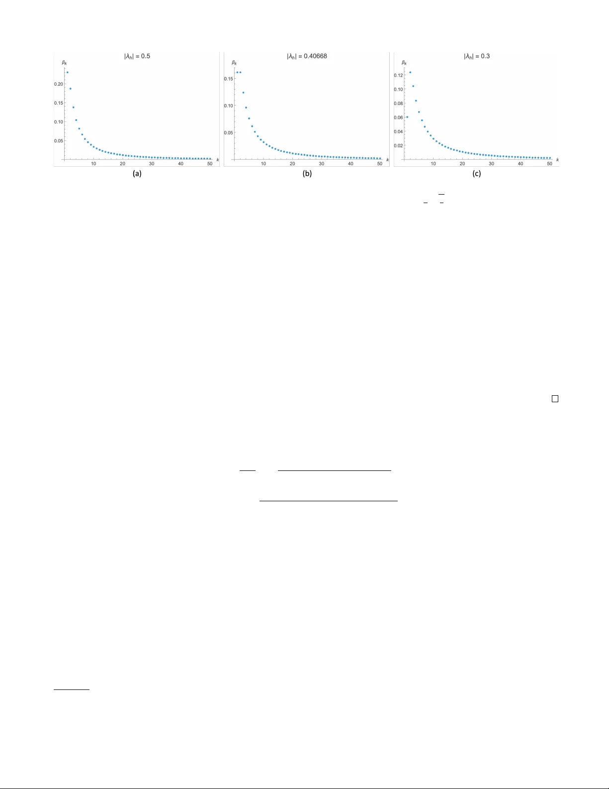
Ultra violet Fixed P oin t in Co v arian t Lo op Quan tum Gra vit y Muxin Han ∗ Dep artment of Physics, Florida Atlantic University, 777 Glades R o ad, Bo ca R aton, FL 33431, USA and Institut f¨ ur Quantengr avitation, Universit¨ at Erlangen-N¨ urnb er g, Staudtstr. 7/B2, 91058 Erlangen, Germany W e in vestigate the ultraviolet b ehavior of 4-dimensional Lorentzian cov ariant Lo op Quan tum Gra vity (LQG) and address the problem of inﬁnite ambiguities relating to the triangulation dep en- dence of spinfoam amplitudes. W e consider the complete LQG amplitude that summing spinfoam amplitudes ov er 2-complexes. By introducing spin-netw ork stacks and their cov ariant extension, spinfoam stacks, the summation ov er complexes is partitioned into distinct families. W e demon- strate that the theory exhibits a condensation phenomenon, where quantum geometry condenses to a dominant small spin conﬁguration. W e identify a candidate ﬁxed p oint controlling the ultraviolet (small spin) regime of cov ariant LQG. At this ﬁx p oint, the complete LQG amplitude dynamically reduces to a top ological theory at leading order, and the inﬁnite ambiguities of triangulation dep en- dence reduces to a ﬁnite set of b oundary co eﬃcien ts asso ciated with a ﬁnite basis of 3-dimensional b oundary blo c ks. These results provide a deﬁnition for the con tinuum limit of spinfoam theory at the fundamental level. In cov arian t lo op quantum gravit y (LQG), the transition am plitudes b etw een spin-net work b oundary states are deﬁned via a spinfoam path integral, wherein one sums ov er states that decorate a chosen 2-complex [1 – 3]. The 2-complex serves as a discretization of spacetime, dual to a cellular decomp osition; for any ﬁxed choice of 2-complex, the amplitude is sp eciﬁed in a well-deﬁned manner. Ho wev er, a fundamen tal challenge arises from the fact that the discretization is not merely a tec hnical device or auxiliary regulator: the transition amplitude dep ends on the c hoice of 2-complex, and mo diﬁcations to the underlying complex, such as reﬁning or altering its combinatorial structure, generally yield inequiv alen t amplitudes. So the theory has inﬁnite ambiguities corresp onding to choices of 2-complexes. A useful approach tow ard resolving the issue is to sum ov er p ossible 2-complexes (se e e.g. [4–6]). Nev ertheless, the ambiguities of the theory persist within this framew ork: for eac h 2-complex contributing to the sum, one ma y assign an independent weigh t, the most general sum includes an inﬁnite collection of arbitrary coeﬃcients, eac h corresp onding to a distinct 2-complex. The resulting microscopic parameter space is still inﬁnite-dimensional. The situation structurally analogous to that of a nonrenormalizable quantum ﬁeld theory , in which inﬁnitely man y couplings must b e ﬁxed to deﬁne the theory . T o address this am biguit y in the contin uum limit, a v ariety of renormalization group (R G) approac hes ha ve been dev elop ed for LQG and related mo dels [7 – 9]. The goal of these approac hes is to identify the ultra violet (UV) ﬁxed p oint, whic h should ensure the theory’s fundamental indep endence of discretization choice. In spinfoams, coarse-graining via tensor netw ork and geometric tec hniques aims to identify ﬁxed p oints where the theory b ecomes indep enden t of microscopic details [10 – 15]. Complementing the cov ariant approach, a Hamiltonian renormalization program is dev elop ed for canonical LQG, tow ard a lattice-indep enden t ﬁx p oin t [16–19]. In Group Field Theory , R G metho ds hav e revealed renormalizable mo dels and emergent condensed geometric phases [20–26]. The causal dynamical triangulations (CDT) program sums o ver triangulations to recov er smooth spacetime via second-order phase transitions [27 – 29]. These ideas connect with the broader asymptotic safety scenario, which p ostulates a non-Gaussian UV ﬁxed p oint underlying quan tum gra vity [30–38]. The central result of this article is that, with a nonp erturbative summation organized by spinfo am stacks , w e iden tify a candidate ﬁxed point controlling the ultra violet (UV) regime of co v ariant LQG (Fig. 1). At this ﬁx p oint, the complete bulk LQG amplitude that summing o ver 2-complexes dynamically reduces to a top ological theory at leading order, and the dep endence on ambiguous weigh ts of complexes collapses from inﬁnitely many co eﬃcients to a ﬁnite set of b oundary co eﬃcients asso ciated with a ﬁnite basis of b oundary blo cks . These results provide a deﬁnition for the con tin uum limit of spinfoam theory at the fundamen tal level. Stacks.– The starting p oint is to build the summing-o v er-graph structure into the kinematics. On a spatial slice, a con ven tional spin-net w ork state lives on a ﬁxed graph. W e instead consider a family F (Γ) of graphs generated from a r o ot gr aph Γ. A root graph is a closed oriented graph with n o des n and orien ted links l such that any pair of no des is connected b y at most one link (the pair of no des can be iden tical in the case of a loop). The family F (Γ) contains graphs Γ(  p ) given by stac king p l ∈ Z + parallel links on each ro ot link l ⊂ Γ. A spin-network stack is a general sup erposition of spin-netw ork states on Γ(  p ) by summing ov er all  p = { p l } l ⊂ Γ , spin assignments  k , and intert winer lab els. ∗ hanm(At)fau.edu 2 FIG. 1. Schematic UV ﬁxed-p oin t signal: in a large-cutoﬀ regime the bulk stack amplitude localizes and b ecomes eﬀectiv ely triangulation indep endent, leaving ﬁnitely man y b oundary data. Geometrically , stac k ed links represen t an arbitrarily ﬁne subdivision of the corresp onding face in the dual cellular picture: a single “ﬂux line” is replaced by multiple strands carrying quanta of area. Because stack ed strands are ph ysically indistinguishable, we imp ose p erm utation inv ariance by pro jecting onto the subspace of states that are in v arian t under p ermutations of stack ed links on eac h l . This b osonic pro jection is motiv ated by the fact that discrete p erm utations are part of the gauge redundancy asso ciated with diﬀeomorphisms [39, 40]. The resulting b oundary Hilb ert space, spanned by permutation-in v ariant superp ositions ov er all  p , is the minimal enlargement needed to represen t arbitrarily ﬁne subdivisions while k eeping a ﬁxed ro ot combinatorics [41, 42]. P ermutation inv ariance implies that states are lab elled by unordered tuples of spins; this is why the co v arian t sums later admit a b osonic o ccupation-n um b er description. A spinfoam is understo od as a cov ariant history of a spin-netw ork: starting from a three-dimensional spin-netw ork, its links l and no des n evolv e in to faces f and edges e in four spacetime dimensions. A r o ot 2-c omplex K is deﬁned suc h that for ev ery b oundary cycle of a face f , the face m ultiplicit y is p f = 1 and no t w o faces share the exact same b oundary cycle. The cov ariant history of stac k ed links is stacke d fac es : for a giv en root 2-complex K , w e generate a family F ( K ) of complexes K (  p ) by replacing eac h ro ot face f with p f iden tical copies, all sharing the same orien ted b oundary cycle as f . Stacking th us subdivides dual cellular faces while preserving the 1-sk eleton. W e associate to eac h ro ot face a complex coupling λ f ∈ C and regulate the spin sums by a cutoﬀ A f : for the p f stac ked faces on f carrying SU(2) spins k 1 / 2 , . . . , k p f / 2, we impose P p f i =1 E k i ≤ A f , with a ﬁxed positive and p olynomially increasing sequence E k (e.g. E k = k ( k + 2)). These couplings λ f pla y a role analogous to fugacities: they w eigh t how strongly the sum explores reﬁnemen ts of each face. With these ingredients w e deﬁne the stack amplitude as a sum ov er complexes in the family: A K = X  p   Y f ⊂K λ p f f   A  K ,  p  , (1) where A ( K ,  p ) is the Lorentzian EPRL/KKL amplitude on the complex K (  p ), adapted to the p erm utation-in v arian t b oundary states. In the EPRL-KKL amplitude, the sum ov er spins for each stack of faces is regularized b y imp osing the cutoﬀ A f . The b oundary state of stac k amplitude is a spin-netw ork stack. In the stack amplitude, the summation ov er complexes within each family F ( K ) is gov erned solely b y the coupling constan ts { λ f } . This constraint enables us to pinpoint the UV ﬁxed point: the ﬁx point is disco v ered exactly on the submanifold of the inﬁnite parameter space where these w eigh ts are given by the couplings { λ f } . Allowing for more general weigh ting schemes amounts to perturbing a w a y from this ﬁxed-p oint. Crucially , the UV regime under consideration corresp onds to the small-spin re gime , which is opp osite to the large- spin (semiclassical) limit: the condensation mechanism to b e discussed b elo w keeps the dominant spins at a small nonzero spin k 0 / 2 even for large A f . The cutoﬀ A f pro vides the large parameter that leads to an expansion of the spinfoam path in tegral. The controlled expansion parameter is A h /E k 0 , so one can take the cutoﬀ large while holding ﬁxed the t ypical microscopic area scale through k 0 . In the full spinfoam theory , the cutoﬀs A f should b e understo o d as large but ﬁnite constants, intuitiv ely related to the bare cosmological constant [43]. Consequently , a signiﬁcant 3 suppression of ﬂuctuations in the expansion only o ccurs when A h /E k 0 is large, which for any ﬁnite A h corresp onds to small k 0 . Therefore, the vicinity of the ﬁxed point is the regime of small k 0 , where the topological theory is at the leading order. The smallness of k 0 iden tiﬁes this ﬁxed p oin t as ultra violet, since k 0 is prop ortional to the exp ectation v alue of the quan tum area. A precise characterization of the notion of scale is essential in bac kground-indep enden t quantum gravit y . Unlike con ven tional quantum ﬁeld theory , where length or energy scales are referenced with resp ect to a ﬁxed background geometry , in quan tum gravit y the geometry itself is dynamical, necessitating a revised deﬁnition of scale. In the framew ork of cov ariant LQG, spin v ariables are naturally related to geometric scales, as they corresp ond to the quan tization of area. How ev er, since spins are themselves dynamical v ariables in LQG, it is appropriate to identify the exp ectation v alue of the spin with the physical scale characterizing the regime of the theory . In this context, large expectation v alues of spin corresp ond to the IR regime, while small exp ectation v alues deﬁnes the UV regime. Sp eciﬁcally , the condensation spin k 0 / 2 discussed abov e is the expectation v alue of the spin in the path in tegral. Thus, the UV regime is c haracterized by a small k 0 , while the IR regime corresp onds to a large k 0 . T o address the original triangulation dependence problem, w e still need to sum ov er inequiv alen t ro ot 2-complexes with the same b oundary graph Γ = ∂ K . This in tro duces the microscopic am biguity co eﬃcien ts c K , one for each ro ot complex, A = X K : ∂ K =Γ c K A K . (2) Without further input, Eq. (2) app ears to b e an in tractable deﬁnition of the dynamics, since the space of ambiguities { c K } and { λ f } is inﬁnite dimensional. The purpose of our analysis is to show these inﬁnite am biguities are remo ved at the UV ﬁx point. A b oson gas of fac es.– The key mec hanism is already visible at the lev el of a single stac k of in ternal faces h . Because the stac ked faces are indistinguishable, the sum ov er spins on a stack can b e reorganized in terms of o ccupation n umbers, as for a nonin teracting Bose gas. T echnically , the stac ked face amplitude ω bos h in the stack amplitude can b e computed by Laplace transform metho d: The Laplace transform of ω bos h is a b osonic grand-canonical partition function Ξ h ( s ) (where s plays the role of an in v erse temperature) of the form Ξ h ( s ) = ∞ Y k =1 1 1 − λ h τ ( h ) k ( g h ) e − sE k − 1 , (3) where k/ 2 labels the SU(2) spin, g h = { g v e } v ⊂ ∂ h are half-edge SL(2 , C ) holonomies around ∂ h , and τ ( h ) k ( g h ) is d k times a simplicit y-pro jected SL(2 , C ) character and satisﬁes a uniform bound | τ ( h ) k ( g h ) | ≤ d 2 k , with d k = k + 1. Expanding Eq. (3) yields a sum ov er o ccupation n umbers { n k } k ≥ 1 with weigh ts Q k [ λ h τ ( h ) k ( g h ) e − sE k ] n k , making the Bose-gas structure explicit. The corresp onding microcanonical ω bos h is the in v erse Laplace transform ω bos h = P ˆ T +i ∞ T − i ∞ d s 2 π i s e A h s Ξ h ( s ) , (4) where T lies to the righ t of all p oles of Ξ h and P denotes principal v alue. As a side remark: Equation (3) has a direct ph ysical interpretation. F or ﬁxed k , the single-face factor λ h τ ( h ) k ( g h )e − sE k pla ys the role of a single-particle partition function. More concretely , for the choice E k = k ( k + 2), which matc hes the energy spectrum of 2d SU(2) Y ang–Mills theory on a disk, the single-face factor can be iden tiﬁed with the partition function of the Y ang–Mills theory on a disk with a b oundary condition determined by k and the b oundary holonomy g h . Thus Ξ h describ es a grand-canonical ensemble of indistinguishable w orld-sheets carrying 2d gauge theory , stac ked o ver the root face. This statistical-mec hanics viewp oint is an eﬃcient w ay to extract the large-cutoﬀ b eha vior of the face factor from the analytic structure of Ξ h . The key p oint is that the same condition maximizing statistical weigh t enforces a geometric constraint. The b ound | τ ( h ) k ( g h ) | ≤ d 2 k is saturated only when the wedge holonomies reduce to SU(2) elemen ts and the face holonom y is ± I : g − 1 v e g v e ′ ∈ SU(2) , − − − − − − → Y ( v ; e,e ′ ) ⊂ ∂ h g − 1 v e g v e ′ = ± I , (5) As A h gro ws, the in v erse Laplace transform is dominated by residues at the poles of Ξ h ( s ) with largest real parts. These p oles o ccur precisely on lo cus of g h satisfying (5). In this wa y , the state sum for internal faces act as nonp erturbative 4 ﬁlters: generic SL(2 , C ) holonomies are suppressed, while the SU(2) subsector is enhanced. This provides the origin of the path integral lo calization derived b elow. Condensation spin and the UV sc ale.– The p oles of Ξ h ( s ) are giv en by s h ( k , m, g h ) = ln  λ h τ ( h ) k ( g h )  + 2 π i m E k , (6) where ln( · ) is the principal logarithm. Here k ∈ Z + and m ∈ Z . The leading contribution to ω bos h is go v erned by the global maximum of Re( s h ( k , m, g h )) and th us relates to a c ondensation spin k 0 / 2 satisfying β k 0 ( λ h ) = sup k ≥ 1 β k ( λ h ) , β k ( λ h ) = ln  | λ h | d 2 k  E k . (7) The situation is directly analogous to Bose–Einstein condensation: b ey ond a critical fugacity the ensem ble accumulates in the low est a v ailable energy lev el, here lab eled by k 0 . In geometric terms, the spin k 0 / 2 sets the typical quan tum area scale selected by the state sum. Indeed, ev aluating Eq. (4) by residues at the dominant p ole yields the leading b ehavior ω bos h ( A h ; g h , λ h ) ∝ [ λ h τ ( h ) k 0 ( g h )] A h /E k 0 , up to a subexp onential prefactor and corrections suppressed faster than any p o wer of A − 1 h . The exp onent p h := A h /E k 0 ≫ 1 can be read as the occupation num b er of faces in the condensate, in direct analogy with Bose–Einstein condensation: the cutoﬀ A h pla ys the role of a total “energy” stored in p h quan ta eac h of “energy” E k 0 . A large ratio A h /E k 0 pla ys a role analogous to the thermodynamic limit: it suppresses ﬂuctuations a w a y from the dominant contribution, and it is in fa vor of small k 0 . In this sense the condensation mechanism selects a UV regime (with small t ypical area). The condensation spin k 0 / 2 con trols the dominant microscopic scale. Since in LQG spin lab els quanta of area, condensation to small k 0 implies that a macroscopic area is obtained as a sup erp osition of man y microscopic quantum areas rather than by exciting a single large spin. As | λ h | decreases, the maximizer k 0 shifts to larger k and ev entually all β k ( λ h ) ≤ 0 or close to zero, so the condensed regime disapp ears, and the stack sum reduces eﬀectiv ely to the spinfoam amplitude on the ro ot 2-complex, corresponding to an infrared description. L o c alization of stack amplitude.– The stack amplitude (1) generated from a ro ot complex K with internal faces h and b oundary faces b can b e written as A K = ˆ dΩ( g ) Y h ω bos h ( g ) Y b ω bos b ( g ) , (8) whic h is an integral ov er the bulk holonomies g v e with pro duct SL(2 , C ) Haar measure dΩ( g ), mo dulo gauge freedom. The factor ω bos b is the amplitude asso ciated to the stack of b oundary faces. By the leading b ehavior of ω bos h , the stac k amplitude b ecomes a stationary-phase form, with the eﬀective action S ( g ) = P h A h E k 0 ln h τ ( h ) k 0 ( g h ) /d 2 k 0 i plus a p ositive constan t. The maximum Re( S ) = 0 is reached if and only if the conditions (5) hold on every internal face. Moreo ver, the same condition implies δ g S = 0. W e deﬁne the submanifold C int as the locus in the space of SL(2 , C ) holonomies where the conditions (5) are satisﬁed for all in ternal faces. The submanifold C int is called the critical manifold, since it contain all critical p oin ts of S making dominan t contribution to A K . When A h /E k 0 are uniformly large, the stac k amplitude lo calizes on C int . The structure of C int is transparent. On eac h internal face Eq. (5) restricts all holonomies to SU(2) and ﬁxes the face holonom y to s h I with s h = ± 1. Collecting the signs { s h } labels disjoin t sectors C int = S { s h } C { s h } int . The critical manifold C int con tains the gauge freedom of the SU(2) holonomies. After remo ving these gauge freedom, the remaining degrees of freedom are precisely the mo duli of ﬂat SU(2) connections (up to sign) on the internal 2-skeleton; their dimension is controlled by the fundamental group of the bulk sub complex. In this pap er, w e fo cus on the simply connected K relev an t to the lo cal UV con tinuum limit, then the moduli reduce to only discrete sign sectors. Boundary blo cks and triangulation indep endenc e.– The b oundary face amplitudes ω bos b do not dep end on gauge freedom, when they are ev aluated on C int , so their dep endence on the bulk contin uous degrees of freedom completely drops out: the contribution from each boundary face is constan t on C { s h } int , and they only dep end on discrete sign data induced from the bulk. Concretely , each stack of b oundary faces b acquires a lab el ς b ∈ { 0 , ± 1 } determined b y the induced signs of holonomies along the internal edges in ∂ b . Here, internal edges are edges that do not connect to the boundary . The v alue 0 corresp onds to the sp ecial case that b do es not hav e any internal edge, then no sign dep endence remains. By the one-to-one corresp ondence b etw een b and boundary link l of the ro ot graph Γ = ∂ K , we iden tify ς l = ς b . Collecting these lab els giv es ς ∈ { 0 , ± 1 } |L| , where |L| is the num b er of links in Γ. The asymptotics of the stack 5 amplitude b ecomes a ﬁnite sum A K = X ς b ς ( K ) B ς  1 + O ( A − 1 )  . (9) The b oundary blo cks B ς equals ´ Q ( v ,e b ) d g v e b Q b ω bos b ( g ) restricted onto C int and depend only on b oundary data ( ς , b oundary holonomies and the b oundary couplings). All bulk degrees of freedom are absorb ed into ﬁnitely many co eﬃcien ts b ς ( K ). Equation (9) already exhibits the UV reduction: for ﬁxed b oundary graph, the set { B ς } spans a ﬁnite-dimensional v ector space of dimension 3 |L| . When neglecting O ( A − 1 ), every ro ot complex K with b oundary Γ deﬁnes a vector A K in this space. The crucial step is to return to the complete amplitude (2). Substituting Eq. (9) yields that the complete amplitude is also a vector in the v ector space A = X ς b ς B ς  1 + O ( A − 1 )  , (10) where the r enormalize d co eﬃcients b ς = X K : ∂ K =Γ c K b ς ( K ) (11) pac k age all bulk degrees of freedom including microscopic triangulation dep endence into ﬁnitely many num b ers. This is the nut of the article: at the le ading or der, the inﬁnite ambiguity of summing over 2-c omplexes c ol lapses to ﬁnitely many b oundary c o eﬃcients b ς . T riangulation indep endence here plays the role of scale inv ariance in a background- indep enden t setting, indicating that at leading order the theory sits at a ﬁxed p oin t of the full co v ariant LQG. Sev eral consequences follow immediately . (i) The predictive conten t of the theory at the ﬁxed p oin t is con trolled by a ﬁnite set of parameters { b ς } , despite the inﬁnite microscopic parameter space spanned by { c K , λ f } . (ii) The theory at the ﬁx p oin t is a top ological theory without propagating bulk degree of freedom. The surviving degrees of freedom are edge-mo de-lik e and encoded by ς sectors. The reduction of the bulk partition function to a linear combination of b oundary blocks is c haracteristic of top ological quan tum ﬁeld theories. A standard example is the relation b et w een Chern-Simons theory and tw o-dimensional conformal blocks. (iii) There are tw o standard con tin uum limit strategies in spinfoams: reﬁning a complex versus summing ov er complexes [5, 44, 45]. Here they b ecome equiv alent, b ecause at the level of stac k amplitude, the leading order dep ends only on b oundary blo cks and not on bulk reﬁnemen t details. F rom an eﬀective-ﬁeld-theory p erspective, the co eﬃcien ts b ς in Eq. (10) play the role of renormalized couplings that parametrize the UV completion on the ﬁxed b oundary ro ot graph. Diﬀerent microscopic choices { c K } that yield the same ﬁnite set { b ς } are indistinguishable at short distances: bulk reﬁnemen ts c hange only subleading O ( A − 1 ) terms. Equiv alently , specifying the UV theory reduces to choosing a vector in the ﬁnite-dimensional boundary-blo ck space, rather than an inﬁnite list of triangulation w eigh ts. This turns the contin uum problem into a ﬁnite matc hing problem: one can aim to determine { b ς } from a ﬁnite set of boundary observ ables and then predict the response to arbitrary bulk reﬁnemen ts in the UV regime. Interpr etation and sc op e.– In our analysis, the UV ﬁxed p oint is iden tiﬁed op erationally , instead of being deriv ed from an y R G equation. In the large internal cutoﬀ limit, the complete LQG amplitude b ecomes top ological and triangulation indep endent. It pro vides a concrete notion of UV ﬁxed-p oin t b eha vior in a background-independent theory . Understanding the RG b eha vior then b ecomes a question of determining which deformations are relev an t and induce ﬂo ws aw a y from the ﬁxed p oin t to ward the infrared (IR) regime. This is in analogy with p erturbativ e quantum ﬁeld theories that expands around a UV ﬁxed p oin t, such as perturbative QCD at short distances, although the ﬁx p oin t here is top ological, in contrast to the free-theory ﬁx p oin t in QCD. F rom the broader ph ysics p ersp ective, the result provides a concrete mechanism of ﬁxed-p oint in a background- indep enden t setting. The b osonic condensation to a small spin provides a dynamical selection of a microscopic area scale, while the large-cutoﬀ limit produces a top ological bulk that is insensitive to short-distance discretization. T ogether they realize, in the spinfoam con text, the RG intuition that a UV completion can be predictive even when the microscopic parameter space is inﬁnite dimensional. The boundary blocks provide the ﬁnite set of UV data that ma y be ﬁxed b y matc hing to ph ysical observ ables. F rom the viewp oin t of asymptotic-safety ideas, the UV ﬁxed p oin t suggested here is not a p erturbativ e Gaussian p oin t but an emergent topological phase: lo cal bulk propagation is absent at leading order, y et non trivial boundary data and con trolled deformations remain. This suggests that RG univ ersality in quantum gravit y may b e realized through phases, captured here b y the boundary-blo ck space and by the ﬁnite set of coeﬃcients { b ς } . Conclusion.– W e in tro duced p erm utation-inv arian t spin-netw ork and spinfoam stacks to organize the sum ov er 2-complexes in Lorentzian cov ariant LQG. The state-sum of b osonic stack ed faces admit a reform ulation as grand- canonical partition-function, w hic h yields a condensation phenomena. The condensation spin k 0 / 2 controls the dom- inan t microscopic area scale. F or uniformly large cutoﬀ and small condensation spin, cov arian t LQG reduce to a 6 top ological and triangulation indep endent ﬁx-p oint theory . As a result, the complete amplitude at the ﬁx p oin t b ecomes a ﬁnite linear combination of b oundary blo c ks, so inﬁnite ambiguities of microscopic triangulations reduce to ﬁnitely many b oundary co eﬃcien ts. A natural next step is to turn on the O ( A − 1 ) p erturbations that generate propagating bulk degrees of freedom and to classify which deformations are relev ant and drive the RG ﬂo w tow ard the infrared. Another is to study the b oundary blocks and connect the resulting co eﬃcients to physical observ ables. Ac kno wledgements: This w ork was made p ossible through the supp ort of the W OST, WithOut SpaceTime pro ject (https://withoutspacetime.org), supp orted by Gran t ID# 63683 from the John T empleton F oundation (JTF). The opinions expressed in this work are those of the author(s) and do not necessarily reﬂect the views of the John T empleton F oundation. The author receives supp orts from Center for SpaceTime and the Quantum (CSTQ) and the National Science F oundation through grants PHY-2207763 and PHY-2512890. Organization of the pap er: The remainder of this pap er is organized as follows. Section I in tro duces the framew ork of permutation-in v ariant spin-net work stac ks. Section I I extends this construction to spacetime b y deﬁning spinfoam stac k amplitudes and the complete amplitude. In Section I I I, the state sum of a stac k of internal face is analyzed with the Laplace transform metho d and related to a grand canonical partition function of b oson system. In Section IV, we relate the system to a Bose gas of 2-dimensional Y ang-Mills theories. Finally , in Section V, we demonstrate the condensation of quantum geometry and derive the asymptotic b ehavior of the state sum for large cut-oﬀ. Section VI deriv es the localization of the stac k amplitude onto a critical manifold in the large-cutoﬀ limit. The parametrization of this critical manifold and the non-degeneracy is detailed in Sections VI I. The associated Hessian matrix is discussed in VI II. Section IX establishes the main result: the reduction of the complete amplitude to a ﬁnite set of b oundary blo cks. Section X prov es that the b oundary blo c k is a linear functional ov er the vector space spanned b y spin-net w orks. 7 CONTENTS I. P ermutation-in v ariant spin-netw ork stac ks 7 I I. Spinfoam stac ks 11 I II. State sum 14 IV. 2-dimensional gauge theory 15 V. Condensation of quan tum geometry 17 VI. Lo calization of stac k amplitude 19 VI I. Parametrization of critical manifold 23 VI II. Hessian matrix 26 IX. Boundary blo cks 28 X. Finiteness of boundary block 31 A. Graph of root complex 33 B. The partition function Ξ[ s h ] 34 C. Bound of | τ ( h ) k ( g h ) | 36 D. In verse Laplace transform 37 E. Bound the deriv atives of τ ( h ) k ( g h ) 41 F. On the sum ov er m 44 G. In terchange sum ov er m and in tegral o ver g 48 H. P arametrization of C S int / G int 49 References 51 I. PERMUT A TION-INV ARIANT SPIN-NETW ORK ST A CKS A r o ot gr aph is a closed, oriented graph Γ where any pair of no des are connected by at most one link (the pair of no des can be identical in the case of lo op). W e deﬁne the link multiplicit y to b e the num ber of links connecting a given pair of no des. The link multiplicities of a ro ot graph equal to one. The ro ot graph serves as the basic com binatorial structure underlying our constructions. On such a graph, a spin-netw ork state is sp eciﬁed by assigning to each oriented link l a spin j = k / 2 ( k ∈ Z + ) and to each no de n a normalized in tert winer I n . Mo ving b ey ond a single ro ot graph Γ, one can generate an entire family F (Γ) of graphs by allowing the link m ultiplicity b etw een pairs of neigh b oring no des to increase—that is, by stacking multiple links b et w een the same pair of no des and aligning their orientations (see FIG.2). Each graph in the family , denoted by Γ(  p ), has the link m ultiplicities  p = { p l } l ⊂ Γ (the ro ot graph is Γ = Γ(  1)). F or any spin-netw ork state on Γ(  p ), each of the p l links b et w een a pair of no des carries its o wn spin, and the intert winers b ecome corresp ondingly higher-v alent. A general sup erposition of these states, referred to as a spin-network stack , is constructed by summing ov er all com binations of link multiplicities { p l } l ⊂ Γ , spin assignmen ts  k , and intert winer lab els. A conv entional spin-net work state is just a special case of a stack in which all sup erposition co eﬃcients but one v anish. W e restrict attention to abstract graphs with ordered links, without specifying an y embedding in a manifold. Consequently , issues related to knotting or top ological em bedding are excluded from our considerations. The graphs discussed ab ov e can b e described formally as lab elled m ultigraphs 8 FIG. 2. The spin-netw ork stack. Deﬁnition I.1. A lab el le d multigr aph G is a tuple ( N , L , Σ L , ℓ L ) , wher e: • N denotes the set of no des. • L is a multiset c onsisting of or der e d p airs of no des, e ach c orr esp onding to an oriente d link. A p air of no des may c oincide, in which c ase the link is a lo op. F or e ach p air l ∈ L , the numb er of o c curr enc es is the link multiplicity p l . Al l stacke d links b etwe en the same p air of no des ar e oriente d identic al ly. • Σ L is a ﬁnite sets serving as the alphab ets of link lab els, satisfying | Σ L | = |L| . • ℓ L : L → Σ L is a bije ctive map that assigns a unique lab el to e ach link, with the c onvention that stacke d links c orr esp onding to the same p air l ∈ L ar e arr ange d c onse cutively in the or dering. A r o ot gr aph Γ is a lab el le d multigr aph with L b eing a set, i.e. p l = 1 . Here, m ultiset allows for multiple instances for each of its elemen ts, e.g. { l , l , l , l ′ , l ′ , · · · } , and the m ultiset is w ell- ordered by the map ℓ L . W e use the pair ( l , i ) to lab el the i -th stac ked link on the root link l ⊂ Γ. The lab el i = 1 , · · · , p l corresp onds to the ordering to the stack ed links. The set of multiplicities  p = { p l } l is well-ordered according to the ordering of l . W e deﬁne an map Φ from a labelled multigraph G to a pair (Γ ,  p ): its ro ot graph Γ is obtained b y pro jecting the m ultiset of links L ( G ) on to a set L (Γ) comprising a single representativ e for each group of stac k ed links. Sp eciﬁcally , for each class of stac ked links in L , the pro jection selects the ﬁrst ordered link as the ro ot link. The corresp onding lab elling map ℓ L (Γ) are inherited so that the ordering match those of the original G . F or e xample, this pro jection maps { l , l , l , l ′ , l ′ , · · · } to the well-ordered set { l , l ′ , · · · } . Con versely , given an y pair (Γ ,  p ), the preimage I Γ , p = Φ − 1 (Γ ,  p ) consists of all lab elled multigraphs G that diﬀer only in their c hoice of link lab els—that is, all p ossible orderings of the stac k ed links. T o construct an elemen t G ∈ I Γ , p , start from the ro ot graph Γ and replace each ro ot link l with p l copies in the multiset L ( G ); the ordering of these copies within the multiset is ambiguous. Thus, I Γ , p en umerates all distinct wa ys of ordering the stac ked links. By regarding I Γ , p as an equiv alence class and selecting a distinguished representativ e G = Γ(  p ) via a ﬁxed ordering, Φ establishes a bijection b etw een the set of pairs (Γ ,  p ) and the set of these ordered represen tativ es G = Γ(  p ). W e deﬁne the kinematical Hilb ert space H Kin as the direct sum o v er all lab elled m ultigraphs: H Kin = M G H G , (12) where H G denotes the Hilb ert space of spin-net work states (with nonzero spins) deﬁned on a labelled multigraph G . Eac h multigraph p ossesses a choice of lab elling of its links, and the lab elling is not summed ov er in (12). By the map Φ, each G is iden tiﬁed to the pair (Γ ,  p ), i.e. G = Γ(  p ). Therefore, H Kin admits the follo wing decomp osition H Kin = M Γ H Γ , st , H Γ , st = M  p H Γ(  p ) . (13) Here H Γ , st denote the Hilbert space of all spin-netw ork stack states on a given ro ot graph Γ. Geometrically , a spin-netw ork state on the ro ot graph represents the quantum geometry of a cellular decomp osition of a spatial slice Σ, with each intert winer enco ding a ﬂat-faced p olyhedron whose num b er of faces is given by the no de’s v alence. Stack states generalize this picture: stac ked links divide a ﬂat face into smaller faces, eac h with (in general) non-parallel three-dimensional normals, so that the stack enco des a quan tum sup erposition of cellular geometries with arbitrarily discretized faces [42]. The graph Γ(  p ) p ossesses a symmetry corresp onding to p erm utations of the stac k ed links at eac h root link l ⊂ Γ. Sp eciﬁcally , at every ro ot link l , the p erm utation group S p l acts b y exchanging the p l iden tical links: given an y 9 spin-net work state ψ Γ(  p ) on the graph, we denote by σ ij ( l ) ∈ S p l the p ermutation exchanging a pair of stack ed links i and j at l , the unitary representation U σ ij ( l ) of σ ij ( l ) acting on ψ Γ(  p ) is given by interc hanging the holonomies of the links in the entries U σ ij ( l ) ψ Γ(  p )  · · · , H ( i ) l , · · · , H ( j ) l , · · ·  := ψ Γ(  p )  · · · , H ( j ) l , · · · , H ( i ) l , · · ·  . (14) Equiv alently , the action exc hanges the spins asso ciated to the holonomies H ( i ) l and H ( j ) l and transposes eac h connected in tertwiner. Indeed, if we consider a state where the i -th and j -th stack ed links are colored b y spins k and k ′ resp ectiv ely , ignoring irrelev an t ingredients in the spin-netw ork and follo wing (14), U σ ij : ( I 1 ) ab D k ( H ( i ) l ) a α D k ′ ( H ( j ) l ) b β ( I 2 ) αβ 7→ ( I 1 ) ab D k ( H ( j ) l ) a α D k ′ ( H ( i ) l ) b β ( I 2 ) αβ = ( I 1 ) ba D k ′ ( H ( i ) l ) a α D k ( H ( j ) l ) b β ( I 2 ) β α = ( I T 1 ) ab D k ′ ( H ( i ) l ) a α D k ( H ( j ) l ) b β ( I T 2 ) αβ . In the result, the i -th and j -th stack ed links are colored by spins k ′ and k resp ectiv ely , while the intert winers are transp osed with respect to the corresp onding slots. In terms of Dirac-k et notation, the action can be written as U σ ij    ψ Γ( p ); k,k ′ ; I 1 ,I 2 E =    ψ Γ( p ); k ′ ,k ; I T 1 ,I T 2 E . (15) The permutations U σ extend unitarily to en tire H Kin . Intuitiv ely , this permutation symmetry w ould be a discrete subgroup within the spatial diﬀeomorphism group if these graphs were embedded in a 3d spatial manifold 1 . Viewing the p erm utations as a part of gauge redundancy motiv ates us to p erform a group av erage and pro ject the Hilb ert space H Γ(  p ) on to its subspace e H Γ(  p ) of p ermutation-in v ariant states 2 . W e deﬁne the p ermutation-in v ariant pro jection P on an y spin-netw ork state ψ Γ(  p ) ∈ H Γ(  p ) b y a v erage ov er all permutations of stac k ed links (at each ro ot link) P ψ Γ(  p ) := 1 | G | X σ ∈ G U σ ψ Γ(  p ) ≡ Ψ Γ(  p ) , G = × l S p l , U σ = Y l U σ ( l ) . (16) where | G | denotes the n um b er of elemen ts in G . The resulting p ermutation inv arian t spin-net w ork state Ψ Γ(  p ) spans the subspace e H Γ(  p ) = P H Γ(  p ) . A linear combination of Ψ Γ(  p ) o ver  p is referred to as p erm utation-in v arian t spin-netw ork stac ks. Summing ov er all ro ot graphs, w e construct the total Hilb ert space of p ermutation-in v ariant spin-net work stac ks as H Sym = M Γ e H Γ , st , e H Γ , st = M  p e H Γ(  p ) . (17) F or the p ermutation-in v ariant spin-netw orks e Ψ Γ(  p ) (normalization of Ψ Γ(  p ) ) forming an orthonormal basis, spin lab els on stack ed links at each l are unordered–the basis states are sp eciﬁed b y tuples of spins ( k 1 , . . . , k p l ), with all p erm utations iden tiﬁed. T o designate eac h basis vector uniquely , one may adopt the con ven tion k 1 ≤ k 2 ≤ · · · ≤ k p l for every l (here k i colors the i -th stack ed link), so that ev ery conﬁguration appears once in the basis. Deﬁnition I.2. L et H Γ(  p ) b e the Hilb ert sp ac e of spin-networks on the gr aph Γ(  p ) with link multiplicities { p l } . We deﬁne the subsp ac e of ordered seed states , denote d H Γ(  p ) , sd ⊂ H Γ(  p ) , as the sp an of spin-network states ψ satisfying two c onditions: 1. Spin Or dering: F or every r o ot link l , the assigne d spins satisfy 1 ≤ k 1 ≤ k 2 ≤ · · · ≤ k p l . 2. Stabilizer Symmetry: If G  k ⊂ × l S p l denote the stabilizer sub gr oup le aving the tuple of spin lab els  k invariant, then U σ ψ = ψ for al l σ ∈ G  k . W e denote by K 0 the set of spin conﬁgurations satisfying the spin ordering 1 ≤ k 1 ≤ k 2 ≤ · · · ≤ k p l on all l ⊂ Γ. The Hilb ert space H Γ(  p ) , sd is a direct sum o v er  k ∈ K 0 : H Γ(  p ) , sd = L  k ∈ K 0 H G  k  k Lemma I.1. F or any ψ  k ∈ H G  k  k , we deﬁne the line ar map U : H Γ(  p ) , sd → e H Γ(  p ) by U ψ  k = s | G | | G  k | P ψ  k . (18) The map U is unitary. These two Hilb ert sp ac es ar e unitarily e quivalent. 1 When the spatial manifold is 2-dimensional (in (2+1)-dimensional gravit y), the p erm utation symmetry do es not relate to spatial diﬀeomorphisms. Therefore, if we apply the formalism in this pap er to (2+1)-dimensional gravit y , the stack ed links and faces are distinguishable 2 See also [40]. A similar idea is in [39] for permutations of no des. 10 Pr o of. It suﬃces to pro v e U is surjective and preserves the inner product. W e denote b y K 0 the set of spin conﬁgu- rations satisfying the spin ordering k 1 ≤ k 2 ≤ · · · ≤ k p l on all l ⊂ Γ. Surjectivit y: F or any Ψ ∈ e H Γ(  p ) , we wan t to construct a preimage ψ ∈ H Γ(  p ) , sd suc h that Ψ = U ψ . The spin- net work decomp osition of Ψ ∈ e H Γ(  p ) ⊂ H Γ(  p ) giv es Ψ = P  k ′ Ψ  k ′ with Ψ  k ′ ∈ H  k ′ , where H  k ′ is the subspace of H Γ(  p ) = ⊕  k ′ H  k ′ . Due to inv ariance U σ Ψ = Ψ, w e hav e P  k ′ U σ Ψ  k ′ = P  k ′ Ψ  k ′ . Comparing comp onents in the subspace H σ ·  k ′ , we ﬁnd U σ Ψ  k ′ = Ψ σ ·  k ′ . Therefore, the set of  k ′ in the sum Ψ = P  k ′ Ψ  k ′ is inv ariant under G and decomp osed into orbits of G , so Ψ decomp oses into inv ariant vectors within each orbit of spin conﬁgurations. It suﬃces to consider Ψ = P  k ′ ∈O  k 0 Ψ  k ′ asso ciated with a single orbit O  k 0 generated by an ordered conﬁguration  k 0 ∈ K 0 . W e deﬁne the candidate seed state ψ as the pro jection of Ψ on to the ordered sector follow ed by a rescaling: ψ ≡ s | G | | G  k 0 | Ψ  k 0 (19) First, ψ is in the seed space H Γ(  p ) , sd , b ecause ψ ∈ H  k 0 has ordered spins and satisﬁes U τ Ψ  k 0 = Ψ τ ·  k 0 = Ψ  k 0 for τ ∈ G  k 0 . Second, we verify U ψ = Ψ: Let R b e a set of representativ es for the left cosets G/G  k 0 . Then any σ ∈ G can b e written uniquely as σ = ρτ with ρ ∈ R and τ ∈ G  k 0 . U ψ = s | G | | G  k 0 | 1 | G | X σ ∈ G U σ ψ = 1 | G  k 0 | X σ ∈ G U σ Ψ  k 0 = 1 | G  k 0 | X ρ ∈ R X τ ∈ G  k 0 U ρ U τ Ψ  k 0 = X ρ ∈ R U ρ Ψ  k 0 = X ρ ∈ R Ψ ρ ·  k 0 (20) As ρ ·  k 0 runs through all distinct spin conﬁgurations in the orbit O  k 0 exactly once, U ψ = P  k ′ ∈O  k 0 Ψ  k ′ = Ψ. Th us, U is surjectiv e. Preserving inner product: F or an y ψ = P  k ∈ K 0 ψ  k and ϕ = P  k ∈ K 0 ϕ  k in H Γ(  p ) , sd ⟨ U ψ , U ϕ ⟩ = X  k ∈ K 0 | G | | G  k | ⟨ P ψ  k , P ϕ  k ⟩ = X  k ∈ K 0 | G | | G  k | ⟨ ψ  k , P ϕ  k ⟩ . (21) F or eac h term in the sum, ⟨ ψ  k , P ϕ  k ⟩ = 1 | G | X σ ∈ G ⟨ ψ  k , U σ ϕ  k ⟩ . (22) Since ψ  k and ϕ  k b elong to the ordered sector with spins  k , and U σ maps spins  k to σ ·  k , the inner pro duct ⟨ ψ  k , U σ ϕ  k ⟩ v anishes unless σ ·  k =  k (i.e., σ ∈ G  k ). Thus, the sum restricts to the stabilizer G  k . Since ϕ  k is a seed state (in v arian t under G  k ), U σ ϕ  k = ϕ  k for σ ∈ G  k . 1 | G | X σ ∈ G  k ⟨ ψ  k , ϕ  k ⟩ = | G  k | | G | ⟨ ψ  k , ϕ  k ⟩ . (23) As a result, ⟨ U ψ , U ϕ ⟩ = X  k ∈ K 0 ⟨ ψ  k , ϕ  k ⟩ = ⟨ ψ , ϕ ⟩ . (24) Therefore U is unitary . W e hav e established the identiﬁcation H Γ(  p ) , sd ∼ = e H Γ(  p ) via the isomorphism U . This allows any spin-netw ork state ψ Γ(  p ) ∈ H Γ(  p ) , sd to serve as a represen tative for the corresp onding p ermutation-in v ariant state e Ψ Γ(  p ) = U ψ Γ(  p ) ∈ e H Γ(  p ) . By construction, ψ Γ(  p ) is supp orted only on spin assignments k 1 ≤ k 2 ≤ · · · ≤ k p l for eac h ro ot link l , and can b e represen ted a spin-net work function of holonomies: ⟨  H | ψ Γ(  p ) ⟩ = ψ Γ(  p ) (  H ) ,  H = { H ( i ) l } l ⊂ Γ , i =1 ,...,p l , (25) where H ( i ) l ∈ SU(2) denotes the holonom y assigned to the i -th stac k ed link along l . Extending the isomorphism U to en tire H Sym , we obtain the following represen tation of H Sym in terms of ordered seed states: H Sym ∼ = M Γ e H Γ , st , e H Γ , st ∼ = M  p H Γ(  p ) , sd . (26) 11 I I. SPINF O AM ST ACKS In what follows, w e will dev elop a spinfoam formalism naturally associated with H Sym , as distinct from the spinfoam mo dels of [41, 46] whic h naturally act on H Kin . Giv en that spin-net work stac ks are well-deﬁned in the Hilb ert space and hav e interesting geometric interpretations, it is natural to exp ect that their cov ariant dynamics should b e prop erly incorp orated within spinfoam theory . In the spinfoam framework, a spinfoam is understo o d as a cov ariant history of a spin-net work: starting from a three- dimensional spin-netw ork, its links l and no des n evolv e into faces f and edges e in four spacetime dimensions. These faces and edges are resp ectiv ely assigned spins j f = k f / 2 and intert winers I e , mirroring the assignments on the initial spin-net work. Conv ersely , slicing a spinfoam produces a spin-netw ork state on the corresponding boundary . In general, the faces and edges form a 2-complex, which underlies the deﬁnition of the spinfoam amplitude. Most of the studies on spinfoams focus on a ﬁxed 2-complex, resultin g in amplitudes and predictions that are sensitiv e to this choice. T o dev elop a more complete and robust spinfoam form ulation, how ever, one should seek amplitudes that are independent of the particular 2-complex used. This suggests summing o ver all possible 2-complexes, in line with the structure of LQG’s Hilbert space, where generic states are superp ositions ov er spin-netw orks on diﬀeren t graphs. This motiv ation leads to extending the idea of stacks to the spacetime (cov ariant) setting. A spinfoam stack is deﬁned as a sum o ver spinfoams corresp onding to a family of 2-complexes, with the prop erty that in tersecting an y spatial slice yields a spin-netw ork stack. The amplitude for such a stack–a stack amplitude –is the sum of the spinfoam amplitudes ov er all 2-complexes in this family . More concretely , just as a spin-net work stack is assembled by stacking links onto a root graph Γ, a spinfoam stac k arises by stacking faces on to a root 2-complex K . Deﬁnition I I.1. A lab el le d multi-2-c omplex is a tuple ( G , F , Σ F , ℓ F ) , wher e: • G = ( V , E ) is a gr aph that serves as the 1-skeleton of the c omplex: V is the set of vertic es (0-c el ls). E is the set of e dges (1-c el ls). • F is a multiset of oriente d b oundary semi-cycles r epr esenting the fac es (2-c el ls) f . The semi-cir cle b e c omes a ful l cir cle ∂ f if f is an internal fac e. An oriente d b oundary cycle along ∂ f is a ﬁnite se quenc e of e dges ( e 1 , e 2 , . . . , e k ) fr om E . Each e i is endowe d an orientation by f such that the tar get vertex of e i is the sour c e vertex of e i +1 , forming an oriente d walk in G . F or a given b oundary semi-cycle, the multiplicity p f is the numb er of distinct fac es in F that shar e this exact oriente d b oundary cycle ∂ f . These fac es ar e the stacke d fac es. The stacke d fac es sharing the same b oundary cir cle have the same orientation. • Σ F is a ﬁnite set serving as the alphab et of fac e lab els, satisfying | Σ F | = |F | . • ℓ F : F → Σ F is a bije ctive map that assigns a unique lab el to e ach fac e, with the c onvention that the fac es ar e or der e d by their lab els. The stacke d fac es sharing the same b oundary cir cle ar e arr ange d c onse cutively in the or dering. A r o ot 2-c omplex K is a lab el le d multi-2-c omplex wher e F is a set r ather than a multiset. This implies that for every b oundary cycle ∂ f , the multiplicity is p f = 1 . No two fac es shar e the exact same b oundary cycle. Giv en a ro ot 2-complex K , the family F ( K ) is generated b y increasing the face multiplicities arbitrarily (see FIG.3). A lab elled m ulti-2-complex in F ( K ) with face multiplicities  p = { p f } f is denoted by K (  p ). It is obtained by replacing eac h root face f ⊂ K with p f copies in the multiset F of K (  p ), follo wed by a c hoice of ordering. In the following, we use v , e, and f to denote vertices, edges, and faces of the ro ot complex K . W e distinguish in ternal faces h from b oundary faces b . The internal faces h do not connect to ∂ K . In K (  p ) ∈ F ( K ), the stack ed faces are labelled b y the pair ( f , i ), f = h or b , where i = 1 , · · · , p f corresp onds to the ordering to the stack ed faces. The 2-complex K (  p ) ∈ F ( K ) has the same set of edges and v ertices as the root complex K . The stack amplitude A K sums the spinfoam amplitudes on all complexes K (  p ) ∈ F ( K ). T o organize the sum, eac h ro ot face f is assigned a coupling constan t λ f ∈ C . The amplitude on a given complex K (  p ) ∈ F ( K ) is w eigh ted b y Q f ⊂K λ p f f . A K = X  p Y f ⊂K λ p f f A ( K ,  p ) . (27) The amplitude A ( K ,  p ) generalizes the EPRL-KKL spinfoam amplitude to ensure compatibility with p ermutation in v ariance. In the EPRL-KKL formalism [1 – 3, 47], for any 2-complex such as K (  p ), each edge e betw een a pair of vertices v , v ′ is asso ciated with a pair g v e , g v ′ e ∈ SL(2 , C ), and each edge e b b et w een a vertex v and a b oundary no de n is asso ciated 12 FIG. 3. The spin-netw ork stac k evolv es to the spinfoam stack: The spin-net w ork link l evolv es to the spinfoam face f . the spin-net work no des n 1 , n 2 ev olve to the spinfoam edges e 1 , e 2 . The faces evolving from the dashed links are not shown on this ﬁgure. The leftmost complex is the ro ot complex. The p o wer of coupling constant λ f coun ts the num ber of stack ed faces. with g v e b ∈ SL(2 , C ). F or an y face , we introduced the short-hand notation g h = { g v e } e ⊂ ∂ h and g b = { g v e } e ⊂ ∂ b b eing the collection of group v ariables along the b oundary of the face. Giv en an y f = h or b , all p f stac ked faces share the same boundary edges and depend on the same set of group v ariables g v e ∈ SL(2 , C ). The amplitude asso ciated to a face ( f , i ) ⊂ K (  p ) colored by spin k i / 2 is • Internal face f = h : τ ( h ) k i ( g h ) = d k i T r ( k i ,ρ i ) " − − → Y v ∈ ∂ h P k i g − 1 v e g v e ′ P k i # , ρ i = γ ( k i + 2) , (28) where d k = k + 1 is the dimension of the spin- k / 2 representation of SU(2). At any v ertex v , the edges e and e ′ are, resp ectively , the incoming and outgoing edges according to the face’s orien tation. The trace T r ( k i ,ρ i ) is ov er the Hilbert space H ( k i ,ρ i ) carrying the principal series SL(2 , C ) irrep, whic h can be decomposed into SU(2) irreps b y H ( k i ,ρ i ) = ⊕ ∞ l =0 H k i +2 l . The orthogonal pro jection P k i is from H ( k i ,ρ i ) to the low est SU(2) irrep subspace H k i con taining solutions of simplicity constraint. ρ i = γ ( k i + 2) = 2 γ ( j i + 1) follows from the conv ention in [48] and is a conv enien t choice for the computation in Section VI II, although the result is not aﬀected by a diﬀerent c hoice suc h as ρ i = γ k i . • Boundary face f = b : τ ( b ) k i ( g b ) = d k i T r ( k i ,ρ i ) " − − → Y v ∈ ∂ b P k g − 1 v e g v e ′ P k ! H ( i ) l ( b ) # . (29) where the SU(2) holonomy H ( i ) l ( b ) is along the b oundary link ( l ( b ) , i ) of the face ( b, i ). The orien tation of the holonom y matc hes the orien tation of the b oundary link induced by the face. The EPRL-KKL amplitude is deﬁned by a pro duct of τ ( h ) k i ( g h ) and τ ( b ) k i ( g b ) ov er all faces, follo wed by in tegrating ov er g v e ∈ SL(2 , C ) for all pairs ( v , e ) and summing ov er all spins coloring faces. In particular, at each ro ot face f , we sum o ver k 1 , · · · , k p f for p f stac ked faces on f . T o ensure compatibility with H Sym , w e require that for eac h face f , the p f -tuple of spins ( k 1 , . . . , k p f ) assigned to the stac ked faces satisfy the ordered condition k 1 ≤ · · · ≤ k p f . This ordering mirrors the constraint imp osed on ordered seed states in H Γ(  p ) , sd . It turns out to b e the only restriction needed for spinfoams. Consequently , the b oundary spin data resulting from slicing a spinfoam stack corresp ond to states in H Sym as given b y the representation (26). The summation ov er spins in the spinfoam amplitude A ( K ,  p ) runs ov er all assignments of spins to the stack ed faces that ob ey the ordering condition for each ro ot face f . Ho wev er, summing ov er an inﬁnite range of spins leads to so-called bubble divergences in the spinfoam amplitudes; see, for example, [49 – 52]. In particular, these divergences generally o ccur in A ( K ,  p ) as stac k ed in ternal faces share b oundaries, forming bubble-lik e closed surfaces where the corresponding spins b ecome un b ounded. T o regularize the div ergence, w e introduce a cut-oﬀ sc heme as follows. 13 Let { E k } k ∈ Z + b e a sequence of p ositive in tegers, with E k deﬁned to b e monotonically increasing and to grow asymptotically as k N for some positive integer N as k → ∞ . F or eac h ro ot face f , w e deﬁne a cut-oﬀ function α p f ,  k = p f X i =1 E k i ,  k = ( k 1 , . . . , k p f ) (30) and imp ose that α p f ,  k ≤ A f for some ﬁnite cut-oﬀ A f ≫ 1. This requirement ensures that b oth the face multiplicities p f and the spins are b ounded. In practice, we frequen tly choose E k = k ( k + 2), prop ortional to the quadratic Casimir, for explicit computations. Using the formalism developed ab o ve, the stack amplitude A K can b e written as a function of the boundary SU(2) holonomies  H = { H ( i ) l ( b ) } b,i : A K   A,  H ,  λ  = ˆ dΩ( g ) Y h ω bos h ( A h ; g h , λ h ) Y b ω bos b  A b ; g b ,  H l ( b ) , λ b  (31) ω bos h = ∞ X p h =1 λ p h h ∞ X 1 ≤ k 1 ≤···≤ k p h p h Y i =1 τ ( h ) k i ( g h ) Θ  A h − α p h ,  k  , (32) ω bos b = ∞ X p b =1 λ p b b ∞ X 1 ≤ k 1 ≤···≤ k p b p b Y i =1 τ ( b ) k i  g b , H ( i ) l ( b )  Θ  A b − α p b ,  k  . (33) The function Θ( A f − α p f ,  k ) imp oses the cut-oﬀ on the summations ov er p f and  k , where Θ( x ) is deﬁned as Θ( x ) = 1 for x > 0, Θ( x ) = 0 for x < 0, and Θ( x ) = 1 / 2 for x = 0. The sum ov er 2-complexes K (  p ) ∈ F ( K ) in A K is encoded in Eqs.(32) and (33) through summations o ver p f . The spinfoam amplitude A ( K ,  p ) is obtained by extracting the coeﬃcient of Q f λ p f f in the pow er series expansion of A K . W e mak e several remarks about the stack amplitude A K : • If the coupling constants λ f , λ b satisfy some consistent relations b etw een diﬀerent complexes, the stack amplitude is consistent under cut and gluing b y the same computation as in [41, 53]: If we slice K into tw o ro ot complexes K 1 and K 2 , the consistency of stac k amplitudes under cut and gluing is ˆ d  H A K 1 (  H ) A K 2 (  H ) = A K , K = K 1 ∪ K 2 . (34) The SU(2) holonomies  H are along the stack ed links where K 1 , K 2 are glued back to K . W e denote by d  H the pro duct Haar measure. F or any faces f ⊂ K b eing sliced in to faces b 1 ⊂ K 1 and b 2 ⊂ K 2 , the consistency relation b et ween coupling constants λ f on K and λ b 1 , λ b 2 on K 1 , K 2 is λ f = λ b 1 λ b 2 . When this consistency relation for the coupling constants is satisﬁed, the stack amplitudes obey the consistency condition (34). While these relations help clarify the in terpretation of spinfoams as the histories of spin-net work stac ks through slicing, they are not required for the ﬁxed p oint analysis in this work. • F or an y ro ot face f = h or b , consider a group of stac ked faces that share the same spin v alue. The functions τ ( b ) k i dep ends on i only via k i and H ( i ) , exc hanging H ( i ) and H ( j ) with k i = k j lea ves the pro duct Q p b i =1 τ ( b ) k i in v arian t. More generally , for an y assignmen t of spins  k to the stac ked b oundary faces, there exists a stabilizer subgroup G  k consisting of all p erm utations that preserv e the spin proﬁle  k . The partial amplitudes with ﬁxed b oundary  k in A K are in v ariant under the action of G  k . This property reﬂects the second condition U σ ψ = ψ , σ ∈ G  k , in the deﬁnition of ordered seed states. As a result, the b oundary data of A K , or the b oundary data obtained by slicing A K , match with the spin-netw ork stack states in H Sym sp eciﬁed b y the represen tation (26). • The stack amplitude A K constructed ab ov e is in the holonomy representation, where the boundary state is the generalized eigenstate of holonomy op erators. F or a generic b oundary state ψ ∈ H Sym , the asso ciated stack amplitude is giv en by A K [ ψ ] := ˆ d  H A K (  H ) ∗ ψ (  H ) , (35) where d  H is the product SU(2) Haar measure, and ψ (  H ) is a linear combination of ordered seed states, according to the represen tation (26). 14 • The in tegrand Q h ω bos h Q b ω bos b in A K is inv ariant under a set of con tin uous gauge transformations: g v e → x v g v e u e , x v ∈ SL(2 , C ) , u e ∈ SU(2) . (36) A t eac h v ertex, the SL(2 , C ) gauge freedom leads to a div ergence. W e address this by ﬁxing the gauge: c ho ose a sp eciﬁc edge e 0 ( v ) at each v ertex v , e 0 ( v )  = e 0 ( v ′ ) for v  = v ′ and ﬁx g v ,e 0 ( v ) = I . The integration measure dΩ( g ) reads dΩ( g ) = Y ( v ,e ) d g v e Y v δ  g v ,e 0 ( v )  (37) where d g v e denotes the Haar measure on SL(2 , C ). Under the gauge ﬁxing, the absolute con vergence of A K rely on a mild restriction on the ro ot complexes under consideration, namely , when a sphere is used to slice the neigh b orho od con taining a single vertex v , the resulting intersection graph Γ v on the sphere is required to b e 3-connected [54, 55]. F or the analysis in Section VII I, we imp ose the condition that e 0 ( v ) do es not in tersect the b oundary ∂ K , when K has at least one internal face, i.e. w e require e 0 ( v ) ∈ E int (deﬁned b elow) for all vertex v . This condition do es not imp ose an y restriction on the topology of ro ot complex (see Appendix A for an explanation). • F or our subsequent discussion, it is con venien t to deﬁne the sub complex K − (the interior of K ) as the 2-complex formed exclusively b y internal faces h , with asso ciated internal edges e ∈ E int and their endp oint v ertices, where the set E int collects all edges on the boundary of internal faces. The subcomplex K − is constructed from K by remo ving all b oundary faces b and any edges e b attac hed to the b oundary . In this work, we restrict attention to ro ot complexes K such that, whenever a small sphere is used to cut out a neighborho o d of any v ertex v ∈ K − (the vertex connecting to a b oundary face), the intersection subgraph Γ v , − ⊆ Γ v formed b et ween the sphere and the sub complex K − is alwa ys connected. This requirement will b e important for the technical argumen ts in Section VI and subsequent sections. Note that this requirement is nontrivial only for v ∈ ∂ K − , since for v ∈ ∂ K − , Γ v , − = Γ v has b een assumed to b e 3-connected. Any 2-complex dual to a simplicial complex satisﬁes this requirement. • In this work, we only consider the ro ot complexes K ha ving simply connected interior, i.e. π 1 ( K − ) is trivial, for the technical reason to b e discussed in Section VII. Ph ysically , a trivial fundamental group is v alid for all lo cal patc hes of spacetime. The complete spinfoam amplitude A is obtained by summing these stack amplitudes A K o ver ro ot complexes with compatible b oundaries, eac h p ossibly further weigh ted b y a complex coeﬃcient c K . A = X K c K A K , (38) The ro ot complexes included in the sum satisfy the following conditions: (1) they are simply connected, (2) for every v ertex v ∈ K , the graph Γ v is 3-connected, (3) for ev ery vertex v lying on ∂ K − , the graph Γ v , − is connected, and (4) all hav e identical b oundaries, i.e., ∂ K = Γ for ev ery K . In the sum ov er complexes (38), the inﬁnitely many undetermined co eﬃcien ts c K enco de the triangulation depen- dence of spinfoam theory . In what follows, our main result is to show that, at the ﬁx point that w e disco ver in this pap er, these inﬁnitely many ambiguities are eﬀectiv ely reduced to only a ﬁnite n umber of degrees of freedom. W e note that, in the most general case, the w eights assigned to eac h A ( K ,  p ) in (27) could b e chosen arbitrarily , rather than b eing determined sp eciﬁcally by the coupling constants as in our construction. Ho wev er, we interpret the sp eciﬁc assignmen t of w eights via the coupling constants in (27) as intrin sic to the deﬁnition of the ﬁxed p oin t; any deviation from this prescription would driv e the theory aw a y from the ﬁxed p oint. Fixing these weigh t b y coupling constan ts may also b e viewed as a consistent truncation of the inﬁnite-dimensional parameter space: the theory is deﬁned within the truncated parameter space. The parameter space after the truncation remains inﬁnite-dimensional. I II. ST A TE SUM W e assume the ro ot complex K to hav e one or more internal faces. In order to compute ω bos h of an internal root face h , we apply the following inv erse Laplace transform form ula known as P erron’s formula [56 – 58]: Given t wo sequence { α n } ∞ n =1 and { β n } ∞ n =1 where β n ∈ C and α n > 0, if P ∞ n =1 | β n | e − α n c < ∞ for some c > 0, w e ha ve ∞ X n =1 β n Θ ( A − α n ) = P ˆ T + i ∞ T − i ∞ d s 2 π is e As Ξ( s ) , Ξ( s ) = ∞ X n =1 β n e − α n s , T > c (39) 15 In particular, if Ξ( s ) is meromorphic for Re( s ) > 0, the parameter T > 0 is greater than the real part of all singularities giv en b y the in tegrand. P ´ denotes the principal v alue of the integral. Apply this formula to the state-sum in ω bos h : The sum o v er n in (39) corresponds to the sum o ver p h and k 1 , · · · , k p h , and α n corresp onds to α p h ,  k . The summand β n corresp onds to λ p h h Q p h i =1 τ ( h ) k i ( g h ) with a ﬁxed g h . The permutation symmetric tuple ( k 1 , · · · , k p h ) indicates that the stack ed faces are indistinguishable and ob ey b osonic statistics. The sum o ver symmetric tuples can b e recast as a sum ov er non-negative o ccupation num b ers n k for eac h spin k , such that p h = P k ∈ Z + n k : Ξ( s h ) = ∞ X p h =1 λ p h h ∞ X 1 ≤ k 1 ≤···≤ k p h " p h Y i =1 τ ( h ) k i ( g h ) # e − s h α p h ,  k = X { n k } k ∈ Z + ∞ Y k =1 h λ h τ ( h ) k ( g h ) e − s h E k i n k − 1 , (40) where the subtraction of 1 accounts for the v acuum contribution with p h = 0, corresp onding to all n k = 0. The series is absolutely con v ergent for suﬃcien tly large Re( s h ) > 0. The proof is given in App endix B. The state-sum ω bos h is written as ω bos h = P ˆ T + i ∞ T − i ∞ d s h 2 π is h e A h s h Ξ[ s h ] . (41) The function Ξ[ s h ] is absolutely conv ergen t at every p oint on the integration contour, then we can carry out the sum o ver { n k } in Ξ[ s h ] (see Appendix B for details) Ξ( s h ) = ∞ Y k =1 1 1 − λ h τ ( h ) k ( g h ) e − s h E k − 1 , (42) The integration contour of ω bos h lies to the right of all singularities of (42). T o compute the in tegral of ω bos h , we analytically con tinue Ξ( s h ) in (42) b ey ond the contour and obtain Ξ( s h ) as a meromorphic function for Re( s h ) > 0 (see App endix B). IV. 2-DIMENSIONAL GA UGE THEOR Y The Laplace transform Ξ( s h ) of ω bos h is an analog of grand canonical partition function: Ξ( s h ) = ^ X { n k } k ∈ Z + ∞ Y k =1 Z k ( g h , s h ) n k , Z k ( g h , s h ) = λ h τ ( h ) k ( g h ) e − s h E k (43) The quan tit y Z k ( g h , s h ) is a partition function on a single face with spin k / 2. In the follo wing, w e sho w that Z k ( g h , s h ) is a partition function of 2-dimensional Y ang-Mills (YM) theory with the b oundary condition that relates to k , g h and the pro jection P k of simplicity constraint. The classical action for 2-dimensional Y ang-Mills (YM) theory with a compact gauge group G is giv en by S YM 2 = 1 4 e 2 ˆ Σ d 2 x p | det g | T r( F αβ F αβ ) , (44) where F is the curv ature of a gauge connection A , e is the coupling constant, and g αβ is an arbitrary metric on the 2d surface Σ. In tw o dimensions, any 2-form is prop ortional to the area element so we may write F αβ = f ε αβ , where ε αβ is the area element normalized b y ϵ αβ ϵ αβ = − 2 and f is an adjoint-v alued scalar. Plugging this into the action, w e obtain S YM 2 = − 1 2 e 2 ˆ Σ d 2 x p | det G | T r( f 2 ) . Th us, the action dep ends on the metric only via the area element ε = d 2 x √ det g. Since f is a scalar, the action is in v arian t under all area-preserving diﬀeomorphisms, and the only in v ariants of the geometry on whic h the partition function can depend are the gen us of Σ and its total area. W e quan tize the theory on a cylinder Σ = S 1 × [0 , t ], t > 0. This is equiv alen t to the time evolution of the state on a circle. W e tak e the temp oral gauge A 0 = 0. A t a constan t time slice x 0 = 0, the gauge in v arian t data is the 16 holonom y along the circle U = P exp ¸ S 1 A 1 d x 1 . The Hilb ert space H YM 2 is spanned by L 2 (w.r.t. Haar measure) functions ψ ( U ) satisfying the gauge inv ariance ψ ( U ) = ψ ( g U g − 1 ), for all g , U ∈ G . The Hamiltonian op erator is given b y H ∝ ¸ S d x 1 E 2 1 ∝ L ∆ U where L is the circumference of the circle and ∆ U is the Laplace op erator on G , whose eigen v alues are quadratic Casimirs C 2 ( R ) of irreps R . Given tw o states ψ 1 , ψ 2 ∈ H YM 2 that deﬁne the b oundary condition, the partition function of 2d YM theory on the cylinder equals to the transition amplitude Z YM 2 ( S 1 × [0 , t ]) = ⟨ ψ 2 | e − s ∆ U | ψ 1 ⟩ , s = i 2 tLe 2 , (45) here s is prop ortional to the total area tL of the cylinder. The partition function on a disk D 2 can be obtained from the cylinder partition function b y collapsing one b oundary circle to a single p oin t. This imp oses the b oundary condition U = 1 on that end, corresponding to the c hoice ψ 1 ( U ) = δ ( U ). By δ ( U ) = P R dim( R ) χ R ( U ) where R labels the irrep of G , Z YM 2 ( D 2 ) = ⟨ ψ 2 | e − s ∆ U | 1 ⟩ = X R ⟨ ψ 2 | χ R ⟩ e − sC 2 ( R ) , (46) where C 2 ( R ) is the quadratic Casimir of R . T o relate to our context, we consider G = S U (2) and thus C 2 ( R ) = C 2 ( k ) = k ( k + 2) / 4, and we let D 2 b e the in ternal face h . The circle holonomy U of 2d YM theory is along ∂ h , w e split U in to segment holonomies H ee ′ connecting the middle p oints of t wo neighboring edges e, e ′ , following the orien tation of ∂ h : U = − − − − − → Y ( e,e ′ ) ⊂ ∂ h H ee ′ (47) W e deﬁne the follo wing b oundary state as a function of H ee ′ Ψ ( k,ρ ) [ g h ] = λ h O v ∈ ∂ h ψ ( k,ρ )  g − 1 v e g v e ′  , ψ ( k,ρ )  g − 1 v e g v e ′  ( H e ′ e ) = d k T r ( k,ρ )  P k g − 1 v e g v e ′ P k H e ′ e  ∗ , (48) then we hav e the follo wing relation when we set E k = k ( k + 2): Z k ( g h , s h ) = λ h τ ( h ) k ( g h ) e − s h E k = ⟨ Ψ ( k,ρ ) [ g h ] | e − 4 s h ∆ U h | 1 ⟩ ≡ Z YM 2  D 2 , Ψ ( k,ρ ) [ g h ]  (49) = λ h ˆ Y ( e,e ′ ) dH ee ′ e − 4 s h ∆ U h δ ( U h ) Y v ∈ ∂ h  d k T r ( k,ρ )  P k g − 1 v e g v e ′ P k H e ′ e  (50) This is the partition function of a 2d YM theory on the face h with a b oundary condition deﬁned by Ψ ( k,ρ ) [ g h ]. The partition function is analytically contin ued, so it has a complex area parameter s h ∈ C . The state Ψ ( k,ρ ) [ g h ] couples the 2d gauge ﬁeld A to the external SL(2 , C ) gauge ﬁeld g − 1 v e g v e ′ . The state Ψ ( k,ρ ) [ g h ] is not inv ariant under gauge transformation of H ee ′ , and the partition function implicitly in v olves a pro jection of this state onto the gauge-in v arian t subspace. Statistical ensem ble Stac ked spinfoam faces Ensem ble of YM w orld-sheets A gas of b osonic particles A stack of spinfoam faces ov er h A gas of world-sheets carrying YM theories. A b osonic particle A single stack ed face A single world-sheet Quan tum state k The spin k / 2 carried b y the face State Ψ ( k,ρ ) at the world-sheet b oundary P article energy level ε k E k for deﬁning cut-oﬀ YM energy (quadratic Casimir) C 2 ( k ) Occupation num b er The num ber n k of faces with spin k / 2 The num b er of world-sheets having b oundary Ψ ( k,ρ ) In verse temp erature β s h The complexiﬁed area parameter s ∝ tLe 2 Single particle partition function z k e − β ε k Z k ( g h , s h ) = λ h τ ( h ) k ( g h ) e − sE k YM partition function Z YM 2  D 2 , Ψ ( k,ρ ) [ g h ]  Grand canonical partition function Ξ( s ) = f P { n k } k ∈ Z + Q ∞ k =1 Z k ( g h , s h ) n k f P { n k } k ∈ Z + Q ∞ k =1 Z YM 2  D 2 , Ψ ( k,ρ ) [ g h ]  n k T ABLE I. T able I establishes a dictionary b etw een the statistical ensemble of boson gas, stack ed spinfoam faces, and ensemble of w orld-sheets carrying 2d YM theories. The comparison suggests that w e can interpret Ξ( s h ) as a grand canonical partition function for a gas of faces ov er h carrying YM theories (with complexiﬁed area). Moreov er, the stack ed face amplitude ω bos h , as the in v erse Laplace transform of Ξ( s h ), is the partition function of the corresp onding micro- canonical ensemble. In this statistical ensem ble, the world-sheets are indistinguishable and satisfy bosonic statistics. As w e see below, for λ h is not to o small, the system can accum ulate all world-sheets in the low est energy state (low est spin k = 1), analogous to Bose-Einstein condensation. 17 V. CONDENSA TION OF QUANTUM GEOMETR Y The p oles of Ξ( s h ) are denoted by s h ( k , m, g h , λ h ) with k ∈ Z + , m ∈ Z , λ h ∈ C , g h = { g v e } e ⊂ ∂ h : s h ( k , m, g h , λ h ) = r h ( k , g h , λ h ) + im ν h ( k ) , r h ( k , g h , λ h ) = ln h λ h τ ( h ) k ( g h ) i E k , ν h ( k ) = 2 π E k . (51) Here r h ( k , g h , λ h ) is complex in general. ln[ · · · ] takes the principal v alue of the logarithm. The real part of s h ( k , m, g h , λ h ) do es not dep end on m : R h ( k , g h , λ h ) := Re[ s h ( k , m, g h , λ h )] = Re[ r h ( k , g h , λ h )] = ln h    λ h τ ( h ) k ( g h )    i E k . (52) Giv en g h and λ h suc h that Ξ( s h ) has p oles on the righ t-half plane, ω bos h can be computed b y using the residue theorem, and the dominan t contribution comes from the poles s ∗ with largest real parts ω bos h = " X s ∗ Res s → s ∗ e A h s s Ξ ( s ) #  1 + O ( A −∞ h )  , Re [ s ∗ ] = sup k ln h    λ h τ ( h ) k ( g h )    i E k , (53) where Res s → s ∗ denotes the residue at the p ole s ∗ . The error O ( A −∞ ) term collects the exp onentially suppressed con tribution from non-dominan t poles. The proof of this form ula is given in Appendix D. W e denote by G h the space of g h = { g v e } v ∈ ∂ h , with the gauge ﬁxing g v ,e 0 ( v ) = 1 if e 0 ( v ) ⊂ ∂ h . The function τ ( h ) k ( g h ) satisﬁes the uniform b ound | τ ( h ) k ( g h ) | ≤ d 2 k on G h for eac h k , and the b ound is saturated if and only if g h satisﬁes (see Appendix C or [46]) g − 1 v e g v e ′ ∈ SU(2) , ∀ e, e ′ ⊂ ∂ h, e ∩ e ′ = v , − − → Y v ∈ ∂ h g − 1 v e g v e ′ = ± I . (54) W e denote the subspace of g h satisfying this condition b y C ± h , where C + h corresp onds to the pro duct b eing + I and C + h to − I . W e deﬁne C h = C + h ∪ C − h , where C + h and C − h are disjoint. F or any k ∈ Z + and λ h , R h ( k , g h , λ h ) reaches the maxim um at g h ∈ C h : β k ( λ h ) ≡ E − 1 k ln  | λ h | d 2 k  = sup g h R h ( k , g h , λ h ) . (55) Fixing the v alue of λ h , since β k ( λ h ) → 0 as k → ∞ , for an y inﬁnitesimal ε > 0, there exists k m ∈ Z such that there are only ﬁnitely many k < k m suc h that β k ( λ h ) > ε . The maximum of β k ( λ h ) among k < k m giv es the suprem um for the real part of poles from Ξ( s h ): sup k ∈ Z + β k ( λ h ) = sup k 0, which satisﬁes β ∗ < β k 0 ( λ h ). The function R h ( k 0 , g h , λ h ) dep ends contin uously on g h within the domain V ⊂ G h where τ ( h ) k 0 ( g h )  = 0. When generalizing a w ay from C h , we introduce the following op en neighborho o d of C h U h =  g h ∈ V | R h ( k 0 , g h , λ h ) > β ∗  . (58) Clearly , U h is op en and contains C h . Lemma V.1. s ∗ = s h ( k 0 , m, g h , λ h ) stil l holds on the op en neighb orho o d U h , i.e. R h ( k 0 , g h , λ h ) is stil l the lar gest among al l p oles for al l g h ∈ U h . Pr o of. Since β ∗ = sup k  = k 0 β k ( λ h ) = sup k  = k 0 , g h R h ( k , g h , λ h ), it follo ws that R h ( k 0 , g h , λ h ) > β ∗ ≥ R h ( k  = k 0 , g h , λ h ), for all g h ∈ U h . As a consequence, for any g h ∈ U h , the p oles s ∗ = s h ( k 0 , m, ˚ g h , λ h ) are simple for all m ∈ Z . By computing the residues at the p oles, ω bos h ( A h ; g h , λ h ) = e A h r h ( k 0 ,g h ,λ h ) S h ( A h , g h , λ h )  1 + O ( A −∞ h )  , (59) S h ( A h , g h , λ h ) = 1 E k 0 X m ∈ Z e iA h mν h ( k 0 ) r h ( k 0 , g h , λ h ) + im ν h ( k 0 ) Q h ( k 0 , m, g h , λ h ) (60) Q h ( k 0 , m, g h , λ h ) = Y k  = k 0 1 1 − λ h τ ( h ) k ( g h ) e − s h ( k 0 ,m,g h ,λ h ) E k . (61) Here is sum ov er m is a symmetric limit lim M →∞ P M m = − M · · · due to the principal v alue integral. See App endix F for more discussion ab out this sum. Both functions Q h ( k 0 , m, g h , λ h ) and S h ( A h , g h , λ h ) are smo oth on U h , see Lemmas F.2 and E.4 for pro ofs. Recall that τ ( h ) k ( g h ) is the amplitude asso ciated to a face carrying the spin k / 2. The fact that the amplitude ω bos h is prop ortional to e A h r h ( k 0 ,g h ,λ h ) = [ λ h τ ( h ) k 0 ( g h )] A h /E k 0 indicates that the dominant contribution comes from conﬁgurations where all faces are concentrated at the state k 0 , in analogy with the Bose-Einstein condensation 3 . Here, A h represen ts the total energy and E k 0 is the energy of a face at spin k 0 , so the total n um b er of suc h faces is p h = A h /E k 0 . When λ h is such that the condensation spin k 0 / 2 is small, the condensation phenomenon o ccurs in the UV (i.e., small- j ) regime. Given the LQG relation b etw een spin and quanta of area, when this condensation occurs, the macroscopic area is given by the sup erposition of many microscopic quantum areas. As the coupling constant λ decreases, the condensation spin increases, causing the theory to mov e a wa y from the UV regime. In the limit λ → 0, the spinfoam stack amplitude coincides with the standard spinfoam amplitude, whic h is supp orted on the ro ot complex. 3 Large A h corresponds to a large num b er of identical bosons and thus reduces the ﬂuctuations in the grand canonical ensemble. 19 Lemma V.2. (1) F or al l g h in the c omplement U c h = G h \ U h , ther e exists a c onstant ∆ > 0 and a function C h ( g h , ∆) > 0 , which is c ontinuous in g h and indep endent of A h , such that   ω bos h ( A h ; g h , λ h )   ≤ C h ( g h , ∆) e A h [ β k 0 ( λ h ) − ∆ ] , ∀ g h ∈ U c h . (62) (2) F or al l g h ∈ G h , and for any (inﬁnitesimal) ε > 0 , ther e exists a function C h ( g h , − ε ) > 0 , which is c ontinuous in g h and indep endent of A h , such that   ω bos h ( A h ; g h , λ h )   ≤ C h ( g h , − ε ) e A h [ β k 0 ( λ h )+ ε ] , ∀ g h ∈ G h . (63) Pr o of. (1) Recall the deﬁnition of U h in (58). W e consider g h ∈ U h . There are tw o cases for k = k 0 : (1) If g h / ∈ V , i.e. τ ( h ) k 0 ( g h ) = 0, there is no p ole with p ositiv e real part associated with k 0 . (2) If g h ∈ V but g h / ∈ U h , b y the deﬁnition of U h , we hav e R h ( k 0 , g h , λ h ) ≤ β ∗ . (64) F or k  = k 0 , for an y g h and any k  = k 0 , the real part of the poles satisﬁes R h ( k , g h , λ h ) ≤ β k ( λ h ) ≤ sup k  = k 0 β k ( λ h ) = β ∗ . (65) Com bining all these cases, for any g h / ∈ U h , the real part of any p ole s of Ξ( s h ) satisﬁes Re( s ) ≤ β ∗ , and in particular the maximum real part of the p oles satisﬁes Re( s ∗ ( g h )) ≤ β ∗ . W e deﬁne the constan t ∆ > 0 b y ∆ = β k 0 ( λ h ) − β ∗ − ε, (66) for any (inﬁnitesimal) 0 < ε < β k 0 ( λ h ) − β ∗ . Cho ose the contour parameter T = β ∗ + ε = β k 0 ( λ h ) − ∆ with ∆ > 0 for ω bos h , w e hav e the strict inequalit y: T > β ∗ ≥ Re( s ∗ ( g h )). The h yp othesis in Lemma D.3 is satisﬁed for all g h ∈ U c h . As a result, there exists a function C h ( g h , ∆) contin uous in g h suc h that:   ω bos h ( A h ; g h , λ h )   ≤ C h ( g h , ∆) e A h T . (67) (2) F or all g ∈ G h , the maxim um of the real part satisfy Re( s ∗ ( g h )) ≤ β k 0 ( λ h ). The b ound (63) is prov en by c ho osing the con tour parameter T = β k 0 ( λ h ) + ε for an y inﬁnitesimal ε > 0 and use Lemma D.3. VI. LOCALIZA TION OF ST ACK AMPLITUDE Let us apply these results to the stac k amplitude A K = ´ dΩ Q h ω h Q b ω b . W e denote by E int the set of edges not inciden t on the b oundary , and deﬁne the space G int to be the space of { g v e } e ∈ E int with the gauge ﬁxing g v ,e 0 ( v ) = 1 implemen ted. F or an y internal face h , we deﬁne the con tinuous pro jection map p h : G int → G h , { g v e } e ∈ E int 7→ g h , (68) whic h is giv en b y restricting { g v e } e ∈ E int to g h . W e deﬁne the subspaces U int = ∩ h p − 1 h ( U h ) , C S int = ∩ h p − 1 h ( C ς h h ) , where S = { ς h } h , ς h = ± 1 , C int = ∪ S C S int . (69) The subspace C int collects { g v e } e ∈ E int satisfying (54) for all h . The subspace U int ⊂ G int is an op en neighborho o d con taining C int , given by U int = n { g v e } e ∈ E int    R h ( k 0 , g h , λ h ) > β ∗ h , ∀ h o , β ∗ h = sup k  = k 0 β k ( λ h ) > 0 . (70) Lemma VI.1. Given the r o ot c omplex K such that the interse ction gr aph Γ v , − is c onne cte d for al l vertex v (r e c al l the discussion in Se ction II), (1) We denote by U v h = g − 1 v e g v e ′ for v , e, e ′ b elong to the b oundary of an internal fac e h . Any se quenc e of c onﬁgu- r ations in G int that go es to inﬁnity r esults in ∥ U v h ∥ → ∞ for at le ast one h and one v ∈ ∂ h , wher e ∥ U ∥ = p T r( U U † ) for 2 × 2 matrix U . (2) A ny se quenc e in G int tending to inﬁnity r esults in τ ( h ) k ( g h ) → 0 for at le ast one internal fac e h . (3) The sp ac es U int (the closur e of U int ), C S int , and C int ar e al l c omp act. 20 Pr o of. (1) Let { x ( n ) } n ∈ N b e a sequence of conﬁgurations in G int . The space G int is a direct pro duct of man y copies of SL(2 , C ). W e sa y the sequence go es to inﬁnit y if it leav es ev ery compact subset of G int . This is equiv alen t to the condition that the norm div erges 4 : lim n →∞ max v ,e ∥ g ( n ) v e ∥ = ∞ . (71) W e pro ceed by con tradiction. Assume that the sequence go es to inﬁnit y , but U v h remain uniformly b ounded. That is, assume there exists a constant M > 0 suc h that for all n , all v ertices v , and all faces h inciden t to v : ∥ U ( n ) v h ∥ ≤ M . (72) Consider an arbitrary vertex v . Let Γ v , − b e the intersection graph when a sphere is used to cut out a small neigh- b orhoo d of v in the sub complex K − . The no des of Γ v , − are the internal edges e ∈ E int inciden t to v , including the gauge-ﬁxed edge e 0 ( v ). Two no des e a , e b are connected by a link in Γ v , − if they are the b oundary edges of an internal face h at v . W e asso ciate to this link the v ariable U v h = g − 1 v e a g v e b (or its inv erse). The graph Γ v , − is connected. F or any internal edge e inciden t to v , there exists a path in Γ v , − connecting e 0 ( v ) to e . Let this path b e e 0 ( v ) = ϵ 0 , ϵ 1 , . . . , ϵ m = e where ϵ i are the nodes of the graph. W e can express g v e as g v e = g v ϵ 0 ( g − 1 v ϵ 0 g v ϵ 1 )( g − 1 v ϵ 1 g v ϵ 2 ) · · · ( g − 1 v ϵ m − 1 g v ϵ m ) = I · U σ 0 v ,h 0 · U σ 1 v ,h 1 · · · U σ m − 1 v ,h m − 1 , (73) using the gauge condition g v ϵ 0 = I and iden tifying the terms in paren theses as link v ariables U ± 1 v ,h j . Since ∥ U − 1 ∥ = ∥ U ∥ and the norm is sub-m ultiplicativ e ( ∥ AB ∥ ≤ ∥ A ∥∥ B ∥ ). Thus, by the assumption that all ∥ U ( n ) v h ∥ ≤ M . ∥ g ( n ) v e ∥ ≤ ∥ I ∥ m − 1 Y j =0 ∥ U ( n ) v ,h j ∥ ≤ √ 2 M m (74) Since the complex is ﬁnite, the path length m is b ounded. Thus, ∥ g ( n ) v e ∥ is b ounded uniformly for all v , e . This con tradicts the h yp othesis that the sequence go es to inﬁnit y . Therefore, the assumption of b oundedness m ust b e false. There exists at least one pair ( v , h ) suc h that ∥ U ( n ) v h ∥ is un b ounded. Sp eciﬁcally , lim n →∞ max v ,h ∥ U ( n ) v h ∥ = ∞ . (2) Recall the deﬁnition of the function τ ( h ) k in (28). W e deﬁne A ( U ) ≡ P k D ( k,ρ ) ( U ) P k , U ∈ SL(2 , C ), as an op erator on the ﬁnite-dimensional subspace H k . The matrix elements of A ( U ) are matrix co eﬃcien ts of the unitary principal series representation of SL(2 , C ). F or an y non-trivial unitary irreducible represen tation of a non-compact semisimple Lie group, the matrix coeﬃcients v anish at inﬁnit y [59] (see Lemma X.1 for the case of SL(2 , C )). Therefore lim ∥ U ∥→∞ ∥ A ( U ) ∥ k = 0 (75) where ∥ A ( U ) ∥ k is the op erator norm. Let { x ( n ) } b e a sequence in G int tending to inﬁnity . W e hav e shown in the pro of of (1) that there exists at least one pair ( v , h ) such that ∥ U ( n ) v h ∥ is unbounded in the sequence i.e. ∥ U ( n ) v h ∥ → ∞ as n → ∞ . Along this subsequence, lim n →∞ ∥ A ( U ( n ) v h ) ∥ k = 0. Using the sub-multiplicativit y of the trace and op erator norm, we obtain    τ ( h ) k ( g ( n ) h )    ≤ d 2 k   Y v ∈ ∂ h,v  = v    A ( U ( n ) v h )    k      A ( U ( n ) v h )    k → 0 (76) Th us, an y sequence tending to inﬁnit y results in τ ( h ) k → 0 for at least one face. (3) In the formula (70) for U int , the condition R h > β ∗ h is equiv alent to: | τ ( h ) k 0 ( g h ) | > 1 | λ h | e E k 0 β ∗ h ≡ ϵ h > 0 (77) 4 In terms of coordinate, any element g ∈ SL(2 , C ) can be written as g = u 1 e rσ 3 / 2 u 2 , where u 1 , u 2 ∈ SU(2) and r ∈ R . The ”inﬁnity” in SL(2 , C ) corresponds to taking | r | → ∞ . Equiv alently , this asymptotic region can be characterized b y ∥ g ∥ = p 2 cosh( r ) → ∞ . 21 The closure U int is contained in the set deﬁned b y the non-strict inequalities 5 : K = \ h n g ∈ G int       τ ( h ) k 0 ( g h )    ≥ ϵ h o (78) The set K is closed b ecause τ ( h ) k 0 is contin uous. W e now show that K is also b ounded. Assume for contradiction that K is unbounded. Then there must exist a sequence { x ( n ) } ⊂ K with x ( n ) → ∞ . F rom part (2) ab o ve, for such a sequence, there is at least one in ternal face h suc h that τ ( h ) k 0 ( p h ( x ( n ) )) → 0 as n → ∞ . Ho wev er, this contradicts the deﬁning prop erty | τ ( h ) k 0 ( p h ( x ( n ) )) | ≥ ϵ h > 0 for all n , since x ( n ) ∈ K . Thus, K must in fact b e b ounded. As U int is a closed subset of the b ounded set K in the ﬁnite-dimensional manifold G int , it is therefore compact. The compactness of C int and C S int can b e pro v en similarly . W e denote by A K | U the integral restricting on any the compact neigh b orhoo d U satisfying C int ⊂ U ⊂ U int 6 . A K    U = e P h β k 0 ( λ h ) A h ˆ U dΩ( g ) e S (  A,g ,  m,  λ ) Y h S h ( A h , g h , λ h ) Y b ω bos b ( A b ; g b ,  H l ( b ) , λ b )  1 + O ( A −∞ )  , (79) Both Q h S h and Q b ω bos b are smo oth on U . The eﬀective action S is expressed as S = X h A h [ r h ( k 0 , g h , λ h ) − β k 0 ( λ h )] = X h A h E k 0 ( h ) ln " τ ( h ) k 0 ( g h ) d 2 k 0 ( h ) # . (80) The notation k 0 ( h ) emphasizes that the condensation spin k 0 / 2 can be diﬀeren t for diﬀeren t h . W e consider the asymptotic regime that A h /E k 0 ( h ) are uniformly large among internal faces and use the stationary phase appro ximation to compute the integral. Since w e hav e ﬁxed k 0 , we write A h ≡ Aa h for all h and scale A → ∞ . The b oundary data (namely , the function ω b along with A b ,  H , and λ b ) remain ﬁxed. W e employ the stationary phase appro ximation for the integration ov er those v ariables { g v e } e ∈ E int , with E int denoting the set of edges not inciden t on the b oundary: Due to | τ ( h ) k ( g h ) | ≤ d 2 k , it is clear that for all { g v e } e ∈ E int Re( S ) = X h A h E h ln      τ ( h ) k 0 ( g h )    d 2 k 0   ≤ 0 , (81) and Re( S ) = 0 if and only if { g v e } e ∈ E int ∈ C int . Moreov er, to compute ∂ g S , w e deform g v e → g v e (1 + it ( v ,e ) I J J I J ), where J I J is the Lie algebra generator. F or an y pair ( v ∗ , e ∗ ) with e ∗ ⊂ ∂ h , the deriv ativ e of τ ( h ) k ( g h ) with resp ect to t ( v ∗ ,e ∗ ) I J on C int giv es ∂ τ ( h ) k ( g h ) ∂ t ( v ∗ ,e ∗ ) I J      C int =    − id k T r ( k,ρ ) h P k J I J ˚ g − 1 v ∗ e ∗ ˚ g v ∗ e ′ ∗ P k − → Q v  = v ∗ P k ˚ g − 1 v e ˚ g v e ′ P k i id k i T r ( k,ρ ) h P k ˚ g − 1 v ∗ e ′ ∗ ˚ g v ∗ e ∗ J I J P k − → Q v  = v ∗ P k ˚ g − 1 v e ˚ g v e ′ P k i = ± d k T r ( k,ρ )  P k J I J P k  = 0 , (82) where ˚ g v e ∈ C int . The distinction b etw een these t wo cases dep ends on whether e ∗ is oriented as incoming or outgoing at v , according to the orientation of ∂ h . In the second step, the deﬁning condition (54) c haracterizing C int is applied. Therefore, ∂ g S    C int = X h A h E k 0 ∂ g τ ( h ) k 0 τ ( h ) k 0      C int = 0 (83) W e conclude that C int is the critical manifold that collect all { g v e } e ∈ E int satisfying Re( S ) = ∂ g S = 0. 5 Let X be a Hausdorﬀ topological space and f : X → R be a contin uous function. Let ϵ > 0. Deﬁne: U = { x ∈ X | f ( x ) > ϵ } and K set = { x ∈ X | f ( x ) ≥ ϵ } . W e alwa ys hav e the i nclusion: U ⊆ K set Therefore, the equality holds if and only if for every x such that f ( x ) = ϵ , ev ery neighborho o d V of x intersects U (i.e., contains a point y where f ( y ) > ϵ ). How ever, if there exists a p oint x 0 such that f ( x 0 ) = ϵ and x 0 is a lo cal maximum of f , then there exists a neighborho od V of x 0 such that for all y ∈ V , f ( y ) ≤ f ( x 0 ) = ϵ . This implies V ∩ U = ∅ . 6 F or example, choose ϵ ′ h such that ϵ h < ϵ ′ h < d 2 k 0 and deﬁne U = T h { g ∈ G int | | τ ( h ) k 0 ( g h ) | ≥ ϵ ′ h } , then C int ⊂ U ⊂ U int . Moreov er U is a closed subset in the compact set K , so U compact. 22 Asymptotically , the integral in A K | U lo calizes onto the critical manifold C int . Performing the stationary phase expansion for eac h  m , we obtain A K   U = e P h β k 0 ( λ h ) A h A D int / 2 X S F S   A,  λ  ˆ C S int d µ (  σ ) p det ( − H S (  σ ) / (2 π )) ˆ Y ( v ,e b ) d g v e b Y b ω bos b    S , σ  1 + O ( A − 1 )  , (84) where H S (  σ ) = A − 1 ∂ 2 g S   S , σ is the Hessian matrix for the transverse directions to C S int . The notation | S , σ indicates the restriction onto C S int , and  σ denotes the co ordinates on C S int . The function F S (  A,  λ ) is deﬁned as the restriction of e S (  A,g ,  m,  λ ) Q h F h ( g h , m h , λ h ) onto C S int . Its dep endence on g app ears only through τ ( h ) k , which is constan t ov er C S int . Therefore, F S (  A,  λ ) is constan t on C S int . F S   A,  λ  = e S (  A,g ,  m,  λ ) Y h S h ( A h , g h , λ h )    S , σ = Y h X m h e iA h E k 0 [ φ h + π Θ( − ς h )+2 π im h ] ˚ Q h ( m h , λ h , ς h ) β k 0 ( λ h ) E k 0 + i [ φ h + π Θ( − ς h )] + 2 π im h (85) ˚ Q h ( m h , λ h , ς h ) = Y k  = k 0 1 1 − λ h ς h d 2 k e − β k 0 ( λ h ) E k − iE k E k 0 [ φ h + π Θ( − ς h )+2 π m h ] , φ h = Arg( λ h ) . (86) In the form ula (84), e b denotes the edges connecting to the boundary and g v e b ∈ SL(2 , C ). The exp onent D int / 2 > 0 is half of the dimension of the Hessian matrix H S (  σ ). The Hessian matrix H S (  σ ) do es not dep end on g v e b b ecause S only depends on g h . The Hessian matrix also do es not dep end on  m . The nondegeneracy of H S (  σ ) is discussed in Section VII I. The induced measure on C int from the Haar measure Q v ,e  = e b d g v e is denoted b y d µ (  σ ), whose explicit expression is deriv ed in Section VI I. Observ e that the smooth function u = Q h S h Q b ω bos b app earing in the stationary phase in tegral ´ d Ω e S u of (79) dep ends on the scaling parameter A , since S h dep ends on A . It is important to verify that the error term in the stationary phase expansion for (84) remains of order O ( A − 1 ). The stationary phase error is controlled by A − 1 P | α |≤ 2 sup U | D α g u | [60], where D α g denotes a m ulti-index deriv ativ e as deﬁned in Appendix E. By the con tin uit y of p h , the compactness of U implies the compactness of p h ( U ) ∈ U h , then Lemma F.2 establishes that D α g S h is uniformly b ounded by a constant that do es not dep end on A . As a result, P | α |≤ 2 sup U | D α g u | is indep enden t of A , ensuring that the error term is indeed of order O ( A − 1 ). The function |F S | is bounded and p erio dic in A (see App endix F). Therefore, the leading asymptotics of A K | U is exp onen tially growing as A → ∞ 7 : A K   U ∼ e A P h β k 0 ( λ h ) a h A − D int / 2 . (87) Lemma VI. 2. F or any c omp act neighb orho o d e U ⊂ G int that have no interse ction with U int , the inte gr al of A K on e U exp onential ly suppr esses r elative to A K | U , i.e. ther e exists B > 0 such that   A K   e U   ≤ B e β ′ A , β ′ < X h β k 0 ( λ h ) a h . (88) Pr o of. The complement G int \ U int is giv en by the union of regions where at least at one face p h ( g ) ∈ U h , g = { g v e } e ∈ E int . F or an y compact neigh b orhoo d e U ⊂ G int \ U int , we deﬁne W h ≡  g ∈ G int   p h ( g ) / ∈ U h  . (89) The set W h is closed in G int b ecause G h \ U h is closed and p h is contin uous. The set V h is identiﬁed as the intersection V h = e U ∩ W h , so V h is compact in G int , and e U = S h V h . Then we hav e:   A K   e U   ≤ X h ˆ V h dΩ( g )      Y h ω bos h ( g ) Y b ω bos b ( g )      . (90) It suﬃces to b ound each term in this sum individually . Consider a ﬁxed internal face h ′ and the in tegral ov er the region V h ′ . By deﬁnition, for any conﬁguration in V h ′ , the group v ariables g h ′ satisfy g h ′ / ∈ U h ′ . W e ap- ply Lemma V.2. There exists a constan t ∆ > 0 and a function C h ′ ( g h ′ , ∆) contin uous in g h ′ suc h that   ω bos h ′   ≤ 7 The asymptotics dep ends on the choice of E k and the cut-oﬀ function α p h ,k , b ecause the cut-oﬀ A h and the uniform limit A h → ∞ may b e diﬀerent for diﬀerent choices. But our ﬁnal results (140) and (142) does not dep end on the c hoice. 23 C h ′ ( g h ′ , ∆) e A h ′ [ β k 0 ( λ h ′ ) − ∆] , while for other h  = h ′ , there exists a function C h ( g h , − ε ) > 0 con tin uous in g h suc h that   ω bos h   ≤ C h ( g h , − ε ) e A h [ β k 0 ( λ h )+ ε ] , ∀ g h ∈ G h , ∀ ε > 0. Com bining the b ounds, we obtain ˆ V h dΩ( g )      Y h ω bos h ( g ) Y b ω bos b ( g )      ≤ e β ′ A ˆ V h dΩ( g ) C h ′ ( g h ′ , ∆) Y h  = h ′ C h ( g h , − ε ) Y b   ω bos b ( g )   (91) The integrand is a con tinuous function, so the integral giv es a ﬁnite v alue, whose sum ov er h gives the constant B . Moreo ver, β ′ = X h a h β k 0 ( λ h ) − ∆ a h ′ + ε X h  = h ′ a h < X h a h β k 0 ( λ h ) , (92) b ecause ∆ > 0 and ε is arbitrarily small. Let D b e any compact integration domain containing U int . The domain D is the disjoint union of compact sets U ⊂ U int and e U = D \ U int and an op en set U int \ U . The ab o ve shows that the spinfoam integral of A K o ver e U exp onen tially suppresses relative to A K | U . By the regularity of the Haar measure, for any ϵ > 0, we can c ho ose the compact neigh b orho od U so that the measure of U int \ U is less than ϵ , which implies that the contribution of the spinfoam integral ov er U int \ U can b e made arbitrarily small. F urthermore, since the stack amplitude A K is absolutely conv ergen t, its integral ov er the complement of a suﬃciently large compact set D is arbitrarily small. Therefore, for large A , the leading order asymptotics of A K is determined by the b ehavior describ ed in (84), with any other contributions b eing exponentially suppressed. That is, A K = A K   U  1 + O ( A −∞ )  . (93) VI I. P ARAMETRIZA TION OF CRITICAL MANIF OLD In this section, we provide explicit parametrizations of the group v ariables g v e and derive an explicit expression of the measure d µ (  σ ) in (84). Giv en the root complex K , we num b er the vertices b y v = v i , i = 1 , · · · , n . F or every edge e = ( i, j ) for certain i, j = 1 , · · · , n ( i  = j ), the pair of group v ariables g v i e and g v j e are re-lab elled as g ij and g j i . W e use the follo wing decomp osition to parametrize each g ij ∈ SL(2 , C ) g ij = u ij e − ir ij K 3 v ij , u ij = e − iψ ′ ij L 3 e − iθ ′ ij L 2 ∈ SU(2) , v ij = e − iψ ij L 3 e − iθ ij L 2 e − iϕ ij L 3 ∈ SU(2) , (94) where r ij ∈ R and ψ ′ ij , θ ′ ij , ψ ij , θ ij , ϕ ij are Euler angles. T o ﬁx the SL(2 , C ) gauge freedom, w e set r ij = 0 and u ij = v ij = 1 for g ij = g v e 0 ( v ) and still allo w SU(2) gauge transformation at the v ertex. The Lie algebra generators relate to the P auli matrices σ i =1 , 2 , 3 b y L i = 1 2 σ i , K i = i 2 σ i in the fundamen tal represen tation. The Haar measure d g ij reads d g ij = 1 4 π sinh 2 ( r ij ) d r ij d u ij d v ij . (95) where d u ij , d v ij are Haar measures on SU(2). F or an y internal face h , we lab el the v ertices of h by 1 , · · · , m , τ ( h ) k = d k T r ( k,ρ )  g 12 P k g − 1 21 g 23 P k g − 1 32 · · · g ij P k g − 1 ij · · · g m 1 P k g − 1 1 m  (96) where g ij P k g − 1 j i =  u ij e − ir ij K 3 v ij  P k  v − 1 j i e ir j i K 3 u − 1 j i  . (97) is the “holonomy” along the edge ( i, j ). The SU(2) v ariables v ij and v − 1 j i comm ute with P k , and one of them is asso ciated to the SU(2) gauge redundancy . The gauge-inv ariant degrees of freedom is con tained in the com bination v ij v − 1 j i . W e in troduce new v ariables to parametrize this com bination: v ij v − 1 j i = u − 1 ij H ij u j i , (98) 24 where we deﬁne H ij ≡ H e as an SU(2) holonomy along the internal edge e ∈ E int , and H j i ≡ H − 1 ij . In the in tegration measure, one of d v ij or d v j i is redundant and can b e dropp ed; w e identify the remaining measure with d H ij . Notice that when the gauge ﬁxing sets g ij = g v ,e 0 ( v ) = I , this corresp onds to u ij = v ij = 1 and r ij = 0 in the change of v ariables (98). This gauge ﬁxing prescription only sets at most one of v ij or v j i to the identit y for each edge ( i, j ). The SU(2) holonomy H ij is not ﬁxed by the gauge, which follows from the injectivity condition e 0 ( v )  = e 0 ( v ′ ) for v  = v ′ (see Lemma A.1). Recall that the critical manifold is expressed as C int = S S C S int , where eac h sector C S int is lab eled by S = { ς h } h , with ς h = ± 1 assigned to every internal face h . The space C S int consists of collections { g v e } e ∈ E int suc h that g − 1 v e g v e ′ ∈ SU(2) , for all e, e ′ ⊂ ∂ h, e ∩ e ′ = v , − − → Y v ∈ ∂ h g − 1 v e g v e ′ = ς h I , ς h = ± 1 . (99) Let us consider the ﬁrst condition. At any vertex v and any internal face h bounded by v , e 0 (where the gauge ﬁxing g v e 0 = 1 is imp osed) and another edge e 1 connecting v , g − 1 v e 0 g v e 1 ∈ SU(2) restricts g v e 1 ∈ SU(2). F or an y other in ternal face h ′ b ounded by v and e 1 and another edge e 2 connecting v , g − 1 v e 1 g v e 2 ∈ SU(2) restricts g v e 2 ∈ SU(2). The restriction can propagate to all e connecting to v and thus gives g v e ∈ SU(2) for all e ∈ E int , b ecause of the connectivit y of Γ v , − . So we hav e for all edges in E int r ij ≈ 0 . (100) Here and in the follo wing, we use ≈ for the equalit y that holds only on the critical manifold C int . It implies g ij P k g − 1 j i ≈ H ij . (101) Then the second critical point condition in (54) further restricts H ij to satisfy the S -ﬂatness condition, i.e. H 12 H 23 · · · H m 1 ≈ ς h I . (102) for any internal face h . Recall that the sub complex K − (the interior of K ) is the 2-complex consisting of only internal faces h , edges e ∈ E int (on the boundary of h ’s) and vertices as the end points of edges. The signs S = { ς h } h assigned to eac h internal face h must satisfy a compatibility condition with resp ect to the 2-cycles of K − : Let C = P n h h b e any 2-cycle in Z 2 ( K − , Z ). The pro duct of holonomies around the faces in C corresp onds to the holonomy of a trivial lo op in the 1-skeleton, which m ust b e I . This imp oses the following necessary condition for the critical manifold C S int to b e non-empt y: Y h ς n h h = 1 for every generator of H 2 ( K − ) . (103) If this condition fails, then C S int = ∅ ; that is, there are no critical p oin ts for such an assignmen t. Therefore, in the sum o ver S app earing in the stationary phase appro ximation (84), we restrict to those assignments of { ς h } h that satisfy this compatibility condition. In what follo ws, w e assume that the assignmen t of ς h is admissible 8 . The on-shell gauge freedom G int include b oth u ij and H ij → x i H ij x − 1 j , x i ∈ SU(2) , (104) They are called on-shell gauge freedom because the in tegrand e S ´ Q e b d g v e b Q ω b do es not depend on them on C int . Cho osing a base v ertex v ∗ and a maximal spanning tree T in the 1-sk eleton of K − . A maximal spanning tree is a subgraph that connects all v ertices but con tains no loops, and for an y vertex v , there is a unique path P v ∗ → v within the tree T from v ∗ to v . F or a giv e set of { H e } e ∈ E int , we deﬁne the gauge transformation with x i = hol ( P v ∗ → i ) , (105) b eing the SU(2) holonomy made by H e tra veling from v ∗ to the v ertex i . The gauge transformation set H e = 1 along all edges in T . Moreo ver, we adopt { H e } e ∈T → { x i } i  = v 0 to be a change of v ariables 9 . After the change of v ariables, τ ( h ) k can b e generally written as τ ( h ) k = d k T r ( k,ρ )   − − − − → Y ( i,j ) ⊂ ∂ h  u ij e − ir ij K 3 u − 1 ij  P k  x i H ij x − 1 j  P k  u j i e ir j i K 3 u − 1 j i    , (106) 8 F or simply-connected K − , Eq.(103) implies ς h = Q e ⊂ ∂ h ς e , where ς e = ± 1 is deﬁned on each edge. 9 F or an y v ertex i in T , there is a unique v ertex j such that ( i, j ) is an edge and the unique path P v ∗ → i trav els through j . Then x i = H ij x j and d x i = d H ij . 25 where H ij  = 1 only for ( i, j ) ⊂ T . Let us ﬁrst consider a general top ologically non-trivial K − . F or each edge e = ( u, v ) / ∈ T , there is a unique fundamen tal lo op ℓ e based at v ∗ formed by the path P v ∗ → u in T , the edge e , and the path P v → v ∗ in T . All other lo ops in the 1-skeleton of K − are pro ducts of fundamental lo ops, so a minimal set of generator of the fundamental group π 1 ( K − ) can b e chosen to be fundamental lo ops. Then along each generator, there is only a single edge that do es not belong to T . W e denote by L the set of edges along these generators. W e deﬁne a local coordinate c hart in the space of { g v e } e ∈ E int . The co ordinates are given by 10 { r ij } ( i,j ) , { u ij } ( i,j ) , { x i } i  = v 0 , { H l } l ∈ L ,l ∈T , { H e } e ∈ L ,e ∈T . (107) The b o ost parameters { r ij } ( i,j ) and the holonomies { H e } e ∈ L , e ∈T (i.e., those not asso ciated to the spanning tree or cycle generators) describ e directions transverse to the critical manifold C int . The critical p oin t conditions constrain r ij ≈ 0 and determine all { H e } e ∈ L , e ∈T in terms of the remaining v ariables. Recall that C int is a disjoint union of C S int , where S collects the signs in the S -ﬂatness condition (102) at all h .  σ describ ed ab ov e are co ordinates on each C S int but are indep endent of S . Under the gauge that H e = 1 for e ⊂ T and ﬁxing S , the remaining { H e } e ∈ L ,e ∈T are uniquely determined b y using (102) (see Lemma H.2). Ho wev er, diﬀerent S generally leads to diﬀerent { H e } e ∈ L ,e ∈T . One migh t view { H e } e ∈ L ,e ∈T are multi-v alued functions of  σ and b ecome single-v alued on the “co v er space” C int . When π 1 ( K − ) is non trivial, the fundamen tal group π 1 ( K − ) has generators that are sub ject to algebraic relations. These in turn induce non trivial constraints among the holonomies { H l } l ∈ L , l / ∈T . Suc h relations can lead to singularities in the space of SU(2) holonomies that satisfy the S -ﬂatness condition (102), and hence introduce singularities into C S int 11 . As a result, the critical manifold C int ma y fail to b e smooth in general, which complicates the application of the stationary phase approximation. F or these reasons, we will henceforth restrict to the case where K − is simply connected, p ostp oning the general analysis to the future in vestigation. Ph ysically , simple connectivit y is v alid for all lo cal patches of spacetime. With this restriction, the v ariables { H l } l ∈ L , l / ∈T are absen t, so the parametrization (107) reduces to { r ij } ( i,j ) , { u ij } ( i,j ) , { x i } i  = v 0 , { H e } e ∈T , (108) In this parametrization, the v ariables { r ij } ( i,j ) and { H e } e ∈T span the directions transv erse to the critical manifold C int . Restricting to the critical manifold C S int , the conditions r ij ≈ 0 is imp osed, and for all e / ∈ T , the S -ﬂatness constrain t enforces H e = ± I , where the sign is uniquely ﬁxed b y S for each e (see Lemma H.2). The Hessian matrix H arises as the matrix of second deriv ativ es of S with resp ect to these transv erse v ariables. The v ariables { u ij } ( i,j ) , { x i } i  = v 0 , { H e } e ∈ L , e ∈T pro vide coordinates  σ on C int . T o construct the measure on C int , w e replace the non-redundan t d v ij in (95) with d H ij , and decomp ose the pro duct of Haar measures ov er all in ternal edges as Q e ∈ E int d H e = ( Q e ∈T d H e )( Q e / ∈T d H e ). Here, Q e ∈T d H e can be rewritten as Q i  = v ∗ d x i b y the change of v ariables. After removing Q e / ∈T d H e corresp onding the transverse directions, the measure d µ (  σ ) on C S int tak es the form d µ (  σ ) = Y ( i,j ) d u ij 4 π Y i  = v ∗ d x i , (109) whic h is indep endent of S . As a result of the gauge ﬁxing, the integration o ver d u ij asso ciated with the edge e 0 ( v ) is omitted. Correspondingly , the critical manifold has the structure C S int ∼ = SU(2) | E int |−| V | × SU(2) | V |− 1 = SU(2) | E int |− 1 . (110) where | V | denotes the n um b er of v ertices in K . Note that the SU(2) gauge symmetry asso ciated to the base vertex v ∗ do es not contribute to the degrees of freedom parametrizing C S int . The reason is: Lattice SU(2) gauge transformations { x i } act transitively on the space of solutions to the S -ﬂatness condition. All such solutions can b e reached via gauge transformations acting on the reference conﬁguration H e = ± I for all e ∈ E int . How ev er, the gauge transformation at v ∗ corresp onds to the global SU(2) transformation at all vertices by the gauge ﬁxing on T , so it leav es the reference conﬁguration inv ariant and therefore acts as the stabilizer, rather than in troducing an degree of freedom C S int . 10 F or e.g. H e ∈ SU(2), the co ordinates can b e chosen as Euler angles. 11 F or example, on a 2-torus, the relation H A H B = H B H A of holonomies along A and B cycles pro duces a singularity when ( H A , H B ) = (1 , 1). 26 VI II. HESSIAN MA TRIX Using the parametrization (107), we in tegrate out the transv erse co ordinates { r ij } ( i,j ) , { H e } e ∈T in the stationary phase integral (79). The Hessian matrix H is computed with resp ect to the transverse directions. In the follo wing, the coordinate index for the transv erse directions are denoted by α, β . T o simplify the form ulae, w e assume A h = A and k 0 to b e constan t ov er diﬀerent h ( λ h is constant ov er h ), the expression of the Hessian matrix is giv en by H αβ = X h C − 1 0 ∂ α ∂ β τ ( h ) k 0 ( g )    C int , C 0 = d 2 k 0 E k 0 . (111) T o compute the second deriv atives of τ ( h ) k , it is conv enien t to expand e − ir ij K 3 = 1 − ir ij K 3 − 1 2 r 2 ij  K 3  2 + O ( r 3 ) , (112) H e = ˚ H e ( S ) e − i P 3 a =1 t a e L a = ˚ H e ( S )   1 − i 3 X a =1 t a e L a − 1 2 3 X a,b =1 t a e t b e L a L b + O ( t 3 )   , (113) where t a e = − t a e − 1 . The perturbations r ij and t a e represen t directions transv erse to the critical manifold C int , and are asso ciated resp ectiv ely with b o osts on the edges ( i, j ) and with SU(2) holonomies H e for edges e not lying on the maximal spanning tree. On C S int , each H e restricts to ˚ H e ( S ) = ± I , with the sign determined by the choice of S . The resulting Hessian matrix H αβ is a p olynomial of the Barb ero-Immirzi parameter γ . But H αβ b ecomes simpliﬁed if w e only fo cus on the leading order of small γ . In particular, due to the simplicit y constrain t and ρ = γ ( k + 2), w e ha ve [48] 12 ⟨ k , m | P k K 3 P k | k , n ⟩ = − γ ⟨ k , m | L 3 | k , n ⟩ = O ( γ ) . (114) The Hessian matrix is a direct sum of r - r and t - t blocks as γ → 0, due to the oﬀ-diagonals ∂ 2 ∂ r ij ∂ t a mn τ ( h ) k 0    C S int = ± d k 0 T r ( k 0 ,ρ 0 ) h · · ·  u ∓ 1 ij K 3 u ± 1 ij  P k 0  x i ˚ H ij x − 1 j  P k 0 · · · P k 0  x m ˚ H mn L a x − 1 n  P k · · · i = ± d k 0 T r ( k 0 ,ρ 0 ) h · · ·  u ∓ 1 ij P k 0 K 3 P k 0 u ± 1 ij   x i ˚ H ij x − 1 j  · · ·  x m ˚ H mn L a x − 1 n  · · · i = O ( γ ) . (115) where ρ 0 = γ ( k 0 + 2), and the ± sign corresp onds to whether r ij asso ciates with g ij or g − 1 ij . In the second step, w e use the property that all op erators in the trace comm ute with P k except for K 3 . F urthermore, the r - r blo c k is block-diagonal, where each small blo ck asso ciates to r ij at a giv en vertex i . Indeed, at the v ertex i , w e ha ve the diagonal entries X h C − 1 0 ∂ 2 ∂ r 2 ij τ ( h ) k 0    C S int = − X h ;( i,j ) ⊂ ∂ h C − 1 0 ς k 0 h d k 0 T r ( k 0 ,ρ 0 )  P k 0  K 3 K 3  P k 0  = − X h ;( i,j ) ⊂ ∂ h C 1 ς k 0 h + O  γ 2  , C ( h ) 1 = 1 6 d 2 k 0 ( d k 0 + 1) C − 1 0 . (116) In the ﬁrst step, we ha ve used the S -ﬂatness condition (102) and the relation D k 0 ( ς h I ) = ς k 0 h D k 0 ( I ) for Wigner D -matrix on H k 0 . The oﬀ-diagonal en tries are computed X h C − 1 0 ∂ 2 ∂ r ij ∂ r im τ ( h ) k 0    C S int = X h ;( i,j ) , ( i,m ) ⊂ ∂ h C − 1 0 ς k 0 h d k 0 T r ( k 0 ,ρ 0 )  P k 0  K 3 U j im K 3  P k 0 U − 1 j im  = X h ;( i,j ) , ( i,m ) ⊂ ∂ h C 1 ς k 0 h cos ( θ j im ) + O ( γ ) . (117) 12 Recall that here k = 2 j is an integer. 27 Here θ j im is one of the Euler angles of U j im = u − 1 ij u im ∈ SU(2), and U − 1 j im app ears b ecause of (99). F or r im and r j n asso ciate to t w o diﬀerent vertices i  = j ∂ 2 ∂ r im ∂ r j n τ ( h ) k 0    C S int = O ( γ ) . (118) for all m, n , since every o ccurrence of K 3 is enclosed betw een pro jectors P k 0 . Therefore, in the limit γ → 0, the r - r blo c k b ecomes block-diagonal. If the coupling constant λ h is chosen such that the condensation spin k 0 / 2 is an integer, then ς k 0 h = 1 b ecomes constan t, whic h simpliﬁes the Hessian matrix. In this situation, w e can pro ve that the Hessian matrix is non-degenerate in the limit γ → 0. Lemma VI I I.1. When k 0 ∈ 2 Z + , the r - r blo ck is nonde gener ate as γ → 0 if Γ v , − ( v ) is c onne cte d for al l vertic es v . Pr o of. The r - r blo ck is nondegenerate if and only if every small blo cks asso ciated with a vertex is nondegenerate. F o cus on a single vertex v and deﬁne a quadratic form Q ( r ) = P e,e ′ M e,e ′ r e r e ′ with r e , r e ′ ∈ R , where e, e ′ are edges connecting to v but not connecting to the boundary . The matrix M has the diagonals M e,e = − P h ; e ⊂ ∂ h C 1 and oﬀ diagonals M e,e ′ = P h ; e,e ′ ⊂ ∂ h C 1 cos( θ e,e ′ ). k 0 ∈ 2 Z + implies ς k 0 h = 1. The quadratic form can be written as Q ( r ) = − X h,v ∈ ∂ h C 1 T h ( r ) , T h ( r ) = r 2 e 1 ( h ) + r 2 e 2 ( h ) − 2 r e 1 ( h ) r e 2 ( h ) cos( θ e,e ′ ) , C 1 > 0 , (119) where e 1 ( h ) , e 2 ( h ) ⊂ ∂ h are the pair of edges connecting the vertex v . F or any r e ∈ R , we hav e T h ( r ) ≥ 0, and it implies Q ( r ) ≤ 0. Moreov er, Q ( r ) = 0 if and only if T h ( r ) = 0. By gauge ﬁxing r e 0 = 0 for one edge e 0 , T h ( r ) = 0 implies r e = 0 for all e sharing an internal face h with e 0 . By induction, r e = 0 propagates to all edges e by the connectivit y of Γ v , − . The fact that Q ( r ) = 0 implies r = 0 under gauge ﬁxing indicates that the small block associated to v is nondegenerate, so the r - r blo ck is nondegenerate. F or the t - t block of the Hessian, we hav e the diagonal entries: X h C − 1 0 ∂ 2 ∂ t a e ∂ t b e τ ( h ) k 0    C S int = − X h ; e ⊂ ∂ h C − 1 0 ς k 0 h d k 0 T r k 0  L a L b  = − C 2 δ ab X h ; e ⊂ ∂ h ς k 0 h , C 2 = 1 12 d 2 k 0 ( d k 0 − 1) ( d k 0 + 1) C − 1 0 , (120) and the oﬀ-diagonal entries: X h C − 1 0 ∂ 2 ∂ t a e ∂ t b e ′ τ ( h ) k 0    C S int = − X h ; e,e ′ ⊂ ∂ h s e ( h ) s e ′ ( h ) C − 1 0 ς k 0 h d k 0 T r k 0  L a L b  = − C 2 X h ; e,e ′ ⊂ ∂ h s e ( h ) s e ′ ( h ) ς k 0 h , (121) where both e and e ′ are not along the maximal spanning tree T . The sign s e ( h ) = 1 if the orientation of the edge e aligns with the orientation of ∂ h , otherwise s e ( h ) = − 1. Unlik e r ij whic h only asso ciates to the v ertex i , t a e =( i,j ) relates to b oth vertices i and j . So, the t - t blo ck of the Hessian is not blo ck diagonal. Lemma VI I I.2. When k 0 ∈ 2 Z + and K − is simply c onne cte d, the t - t blo ck is non-de gener ate. Pr o of. W e denote b y E v ar to be the set of edges not connecting to b oundary and not b elonging to T . W e deﬁne the follo wing quadratic form asso ciated to the t - t blo ck Q ( t ) = X e,e ′ ∈ E v ar X a,b H ( e,a ) , ( e ′ ,b ) t a e t b e ′ , t a e ∈ R , (122) and set t e = 0 except for e ∈ E v ar . Let us ﬁx, for each face h , a base v ertex v h on its b oundary . F or each edge e ∈ ∂ h , let G h,e b e the background holonomy made by ˚ H e from v h to the target of e along ∂ h (following the face orientation). 28 The holonomy G h,e reduces to G h,e = ± I due to ˚ H e = ± I by the gauge ﬁxing on T . The quadratic form Q ( t ) can b e written as Q ( t ) = X h Q h ( t ) , Q h ( t ) = − C 2 3 X a =1 J a h J a h , J h = X e ∈ ∂ h s e ( h )Ad G h,e t e ∈ su (2) . (123) The condition k 0 ∈ 2 Z + implies ς k 0 h = 1. Q ( t ) ≤ 0 b y C 2 > 0, so Q ( t ) = 0 if and only if for ev ery internal face h , J h = X e ∈ ∂ h s e ( h )Ad G h,e t e = X e ∈ ∂ h s e ( h ) t e = 0 . (124) where t e = P a t a e ( − iL a ). This equation means that the linearized holonomy v ariation δ H ∂ h v anishes at the back- ground { ˚ H e } e for every h . Let v ∗ b e the root vertex of the spanning tree T . F or any edge e ∈ E v ar , deﬁne the loop ℓ e based at v ∗ as follo ws: tra vel from v ∗ to the s ource of e along the unique path in T , trav erse e , and return from the target of e to v 0 along the unique path in T . The linearized holonomy v ariation along ℓ e giv es H − 1 ℓ e δ H ℓ e = Ad G e t e , (125) where G e ∈ SU(2) is the bac kground parallel transp ort from v ∗ to the target of e along the tree part of ℓ e . The terms from edges in T v anish b ecause t e ∈T = 0. On the other hand, the lo op ℓ e equals a pro duct of lo ops ℓ ϵ 1 1 · · · ℓ ϵ k k with ϵ i = ± 1, where ℓ i is the b oundary of an in ternal face h , due to the trivial π 1 ( K − ). Moreov er, recall that Q ( t ) = 0 implies δ H ∂ h = 0. Therefore, w e ha ve δ H ℓ e = 0. Com bining this and (125) yields t e = 0, since Ad G e is an isomorphism of the Lie algebra. This argumen t holds for every e ∈ E v ar . Therefore, Q ( t ) = 0 implies t = 0. Consequently , the quadratic form Q is nondegenerate. This completes the pro of that the t - t block is non-degenerate. Giv en that the Hessian matrix (for k 0 ∈ 2 Z ) is non-degenerate in the v anishing Barbero-Immirzi parameter limit: γ → 0, it is still non-degenerate for a generic v alue of γ , in particular, it is nondegenerate for small γ . Although the nondegeneracy is only pro v en for k 0 ∈ 2 Z , our main result in the following section is v alid in general ev en for degenerate critical p oints: It is shown in [61] that for general oscillatory in tegral J ( A ) = ´ e AS ( x ) φ ( x ) d n x (of the same t yp e as (79)) with an analytic phase and a possibly degenerate critical p oin t x c , there is an asymptotic expansion J ( A ) = e AS ( x c ) X α n − 1 X k =0 c α,k ( φ ) A α (log A ) k , (126) and the leading term is equal to the v alue of the in tegrand at the critical p oint, multiplied b y a non-zero constan t J ( A ) ∼ C e AS ( x c ) φ ( x c ) A − α 0 (log A ) k 0 , (127) for some α 0 , k 0 ≥ 0. Lo calizing the integrand on the critical p oints is the only ingredient that is necessary for deriving our main result. IX. BOUND AR Y BLOCKS In this section, we discuss the b oundary con tribution ´ Q ( v ,e b ) d g v e b Q b ω bos b   S , σ in the asymptotic formula (84). F or a b oundary face b , whose v ertices are labelled b y 1 , · · · , m with m ≥ 2, τ ( b ) k = d k T r ( k,ρ ) h P k g − 1 1 ,e b g 12 P k g − 1 21 g 23 P k g − 1 32 · · · g m − 1 ,m P k g − 1 m,m − 1 g m,e ′ b P k  H l ( b ) i , (128) where g ij are along edges in E int . Use the parametrization discussed in Section VI I g ij P k g − 1 j i =  u ij e − ir ij K 3 u − 1 ij  P k  x i H ij x − 1 j  P k  u j i e ir j i K 3 u − 1 j i  . (129) 29 Restrict τ ( b ) k on C S int and make the follo wing change of v ariables, which leav es the Haar measure d g v e b in v arian t: g 1 ,e b = x 1 e g 1 ,e b , g m,e ′ b = x m e g m,e ′ b , (130) W e obtain τ ( b ) k on C S int : τ ( b ) k ≈ d k T r ( k,ρ ) h P k e g − 1 1 ,e b P k ˚ H 12 ˚ H 23 · · · ˚ H m − 1 ,m P k e g m,e ′ b P k  H l ( b ) i ≈ ς k b d k T r ( k,ρ ) h P k e g − 1 1 ,e b P k e g m,e ′ b P k  H l ( b ) i , ς b = ± 1 , (131) since H e = ± I for every e ∈ E int and D k ( ς b I ) = ς k b D k ( I ) on H k . Therefore, b oth τ ( b ) k and consequently ω bos b tak e constan t v alues on C S int . The sign ς b = ς b ( S ), which is assigned to each b oundary face b , is determined by the bulk sign conﬁguration S = { ς h } . Indeed, for eac h sector S , ς b ( S ) is the pro duct of the signs of the critical holonomies H e ≈ ± I along the in ternal edge e ∈ E int of the b oundary face b , and the sign for each H e is uniquely determined by S (see Lemma H.2). In the case m = 1, the face b is a triangle whose sides are e b , e ′ b , l ( b ). Then b oth τ ( b ) k = d k T r ( k,ρ ) h P k g − 1 v e b g v e ′ b P k  H l ( b ) i (132) and ω b are independent of { g v e } e ∈ E int , so they are constan t on C int . Note that g − 1 v e b g v e ′ b = e g − 1 v e b e g v e ′ b is in v ariant under the gauge transformation at v . W e conclude that for a simply connected K − , ω bos b on C int do es not dep end on  σ . Its dep endence on C int is only through the signs { ς b } b . In addition, we extend the label ς b to ς b ∈ { 0 , ± 1 } and assign ς b = 0 to the case of m = 1. Therefore, ω bos b   S , σ = ˚ ω b,ς b  { e g v e b } ,  H l ( b )  . (133) The explicit expresses are giv en b elow, ˚ ω b,ς b = ∞ X p b =1 λ p b b ∞ X 1 ≤ k 1 ≤···≤ k p b p b Y i =1 ˚ τ ( b,ς b ) k i Θ  A b − α p b ,  k  , (134) ˚ τ ( b, ± ) k = ( ± 1) k d k T r ( k,ρ ) h P k e g − 1 1 ,e b P k e g m,e ′ b P k  H l ( b ) i , ˚ τ ( b, 0) k = d k T r ( k,ρ ) h P k e g − 1 v e b e g v e ′ b P k  H l ( b ) i . (135) When collecting all b oundary faces b , w e denote ς = { ς b } b ∈ Z |L| 3 (136) where |L| is the n umber of links of the b oundary graph Γ = ∂ K , with an one-to-one correspondence b etw een boundary faces b and links in Γ. W e no w relab el all quan tities, replacing the notation asso ciated with the 2-complex b y the corresp onding notation for the boundary graph: ˚ ω b,ς b ≡ ˚ ω l ,ς l , λ b ≡ λ l , p b ≡ p l , A b ≡ A l , ς b ≡ ς l , s b ≡ s l e g v e b ≡ g n , (137) b y virtue of the bijection b etw een each b oundary face b and a link l of the b oundary ro ot graph Γ, as well as the bijection b etw een each e b and a node n in Γ. It is clear that the Haar measure is inv arian t d g v e b = d e g v e b = d g n . Giv en any ro ot graph Γ where the links and no des are denoted b y l and n , we consider Γ as the b oundary of a ro ot 2-complex K . W e deﬁne the vector space V Γ spanned by the follo wing set of functions B ς , which equal the b oundary con tributions ´ Q ( v ,e b ) d g v e b Q b ω bos b   S , σ in the asymptotic formula (84) B ς (  H ) := ˆ Y n ∈ Γ d g n Y l ⊂ Γ ˚ ω l ,ς l  { g n } ,  H l  ,  H = {  H l } l , (138) These functions dep end on SU(2) holonomies  H l = { H ( i ) l } i along the stac ked links o v er l . Note that B ς (  H ) depends on the coupling constants { λ l } l , which are understoo d as ﬁxed parameters. The function B ς dep ends only on the data associated with K \ K − , i.e. the degrees of freedom associated to b and e b . W e can equiv alen tly asso ciate these data to the links and nodes of the b oundary root graph Γ. Accordingly , we refer to them collectively as the b oundary data, consisting of: 30 • ς l ∈ { 0 , ± 1 } for each b oundary ro ot link l . • The boundary SU(2) holonomies  H = { H ( i ) l } l ,i along the stac k ed links on the b oundary root graph Γ. • The boundary area cut-oﬀ A l and coupling constan t λ l . W e call the functions B ς b oundary blo cks and call V Γ the space of b oundary blo cks. The b oundary blo c ks are lab elled b y ς , so the dimension of V Γ is 3 |L| . Eac h of the functions B ς deﬁnes the follo wing linear functional on the v ector space spanned by spin-netw ork states, Cyl ⊂ H Kin , or its p ermutation inv ariant pro jection. B ς [ f ] = lim A l →∞ ˆ d  H B ς (  H ) ∗ f (  H ) , (139) where f ∈ Cyl denotes a ﬁnite linear combination of spin-netw ork states, and d  H represents the Haar measure on the space of SU(2) holonomies on the graph deﬁned by the union of the supp ort graphs of B ς and f . The ﬁniteness of B ς [ f ] is addressed in Section X. As we send the cut-oﬀs A b = A l in ˚ ω l , s l to inﬁnity , there are at most ﬁnitely many terms in B ς that can contribute to B ς [ f ], since f is based on a ﬁnite graph (with ﬁnitely many links). Therefore, for any f ∈ Cyl , there exists a suﬃcien tly large (but ﬁnite) A l for each l such that B ς [ f ] b ecomes indep endent of A l for all larger v alues. Conv ersely , this functional viewp oint also allo ws us to keep A b ﬁnite during the spinfoam calculations ab o v e, without aﬀecting the result when acting on any state in Cyl . With the ab out deﬁnition, we ﬁnd that the leading asymptotics of A K is represented by a ﬁnite linear combination o ver ς A K = X ς b ς ( K − ) B ς (  H )  1 + O ( A − 1 )  . (140) The key p oint is that ω bos b ’s dep endence on C int is only through the signs ς = { ς b } b . Consequen tly , all dep endence of the amplitude on the interior K − of the ro ot complex K is now entirely reduces to a ﬁnite set of co eﬃcients b ς ( K − ). Inﬁnitely many degrees of freedom in the bulk decouples in the limit A → ∞ . These co eﬃcien ts are explicitly deﬁned as sum o v er sign conﬁgurations S compatible with the giv en b oundary data ς , b ς ( K − ) = e P h β k 0 ( λ h ) A h A D int / 2 X S , ς ( S )= ς F S   A,  λ  ˆ C S int d µ (  σ ) p det ( − H S (  σ ) / (2 π )) . (141) Summing ov er inﬁnitely man y 2-complexes K which has the same boundary Γ = ∂ K , the complete amplitude A is still a linear combination ov er b oth ς and s : A = X K ,∂ K =Γ c K A K = X ς b ς B ς  1 + O ( A − 1 )  , b ς = X K ,∂ K =Γ , ς ( K )= ς b ς ( K − ) c K (142) where { c K } K are inﬁnitely many arbitrary coeﬃcients. ς ( K ) = ς means that the b oundary faces of K ha v e the same t yp e as ς . The sum on the left-hand side conv erges if and only if all 3 |L| co eﬃcien ts b ς on the right-hand side con verge as inﬁnite linear combinations of c K . W e mak e several imp ortant observ ations regarding this result: • In the limit A → ∞ , the inﬁnitely many am biguities contained in the co eﬃcien ts c K and λ h b ecome only ﬁnitely man y b oundary co eﬃcients b ς . The bulk ambiguities that disapp ear in this limit decouple from the theory . Since these bulk ambiguities are asso ciated with the triangulation dep endence of the spinfoam, their decoupling implies that the resulting theory is triangulation indep endent. • F or a given b oundary ro ot graph Γ, the b oundary blo cks B ς ∈ Cyl ∗ span a 3 |L (Γ) | -dimensional vector space V Γ . In the limit A → ∞ , the complete amplitude A is represen ted by a v ector in this space. • As A → ∞ , the theory reac hes a ﬁxed point where all bulk degrees of freedom become either frozen or decou- pled. As a signal of ﬁx p oint, the theory in the limit becomes top ological and in v arian t under changing bulk triangulation, with all physical degrees of freedom lo calized on the boundary . • Two approaches hav e b een prop osed for obtaining the con tinuum limit of spinfoam mo dels: summing o ver complexes versus reﬁning them [5, 44, 45]. In our result, the stac k amplitude A K is already free from bulk am biguities. As a result, taking the contin uum limit is trivial, regardless of whether it is performed via summing or reﬁning, and the t w o methods are manifestly equiv alen t. 31 • Our results demonstrate that at the UV ﬁxed p oint A → ∞ , the triangulation-indep enden t theory is well deﬁned. As A − 1 increases aw a y from zero, the theory ﬂo ws a wa y from the ﬁxed point: bulk degrees of freedom b egin to propagate and the system ﬂo ws tow ard the IR regime. • As noted abov e Lemma V.2 and in the deﬁnition of S in (80), the limit A → ∞ can equiv alently b e characterized b y A h /E k 0 → ∞ . In our opinion, the spin cut-oﬀ A should be understoo d as a large but ﬁnite constant in the full spinfoam theory . Intuitiv ely , A is exp ected to relate to the cosmological constant. Consequen tly , a signiﬁcan t suppression of ﬂuctuations (as describ ed by the stationary phase expansion) only o ccurs in the regime where A h /E k 0 is large, which corresp onds to small v alues of the condensation spin k 0 . Therefore, the regime of ﬁnite λ h , where k 0 is small, is the vicinity of the ﬁx p oint. The top ological theory is at the leading order in this vicinit y . The small k 0 indicates that the ﬁxed point is in the UV regime, because k 0 is prop ortional to the exp ectation v alue of the quantum area. X. FINITENESS OF BOUND AR Y BLOCK As a Hilb ert space, the carrier space of the SL(2 , C ) principal series unitary irrep, H ( k,ρ ) , is the subspace of L 2 (SU(2)) made of functions obeying the cov ariance condition F ( e iϕ σ 3 u ) = e ikϕ F ( u ) , u ∈ SU(2) (143) An orthogonal basis of H ( k,ρ ) is made of a subset of Wigner matrices D j k/ 2 ,m ( u ) = ⟨ u | ( k , ρ ) , j, m ⟩ . T o deﬁne the action of SL(2 , C ), we use the Iwasa w a decomp osition: any g ∈ SL(2 , C ) can b e written as g = bu with u ∈ S U (2) and b ∈ B , where B is the subgroup of upper triangular matrices B =  b =  λ − 1 µ 0 λ  , λ ∈ C × , µ ∈ C  . (144) Moreo ver, since u = b − 1 g is unitary , it is useful to notice that b − 1 g = b † ( g − 1 ) † . T o deﬁne the SL(2 , C ) action on H ( k,ρ ) , we use this decomp osition for ug for any u ∈ SU(2) and g ∈ SL(2 , C ): ug = b g ( u ) u g ( u ) , b g ( u ) ∈ B , u g ( u ) ∈ SU(2) (145) Then, the action of g on F ∈ H ( k,ρ ) reads g · F ( u ) = [ λ g ( u )] − k/ 2+i ρ/ 2 − 1 [ λ g ( u ) ∗ ] k/ 2+i ρ/ 2 − 1 F ( u g ( u )) . (146) where λ g ( u ) is the low er right en try of the matrix b g ( u ). Note that the Iwasa w a decomp osition has the gauge freedom b g ( u ) → b g ( u ) e − iϕ σ 3 , u g ( u ) → e iϕ σ 3 u g ( u ). The form ula (146) is gauge inv arian t thanks to the cov ariance condition (143). W e can use this gauge freedom to set λ g ( u ) ∈ R . In this case, λ 2 g ( h ) is the upp er left corner of the matrix ( b g ( u ) − 1 ) † b − 1 g ( u ) = u ( g − 1 ) † g − 1 u † , i.e. λ g ( u ) = h ⟨ 1 2 , 1 2 | u ( g − 1 ) † g − 1 u † | 1 2 , 1 2 ⟩ i 1 2 (147) with | j, m ⟩ the standard basis of the spin j represen tation of SU(2). The ab ov e lemma sho ws explicitly that the matrix co eﬃcien ts of g suppress as te − 2 t as t → ∞ . Lemma X.1. F or any two states F 1 , F 2 ∈ H ( k,ρ ) and any g ∈ SL(2 , C ) , |⟨ F 1 | g | F 2 ⟩| ≤ ξ ( g ) ∥ F 1 ∥ ∞ ∥ F 2 ∥ ∞ (148) wher e ∥ F ∥ ∞ = sup u | F | . , the function ξ ( g ) is given by ξ ( g ) = ξ ( g − 1 ) = 2 t sinh(2 t ) . (149) Pr o of. The explicit expression of λ g ( u ) can be deriv ed by the decomposition g = R − 1 e − t σ 3 R ′ : λ g ( u ) 2 = e 2 t | α | 2 + e − 2 t | β | 2 , Ru † =  α β − β ∗ α ∗  ∈ SU(2) . (150) 32 F or an y tw o states F 1 , F 2 ∈ H ( k,ρ ) , the matrix co eﬃcient of the unitary represen tation of g ∈ SL(2 , C ) is given by ⟨ F 1 | g | F 2 ⟩ = ˆ SU(2) d u λ g ( u ) i ρ − 2 F ∗ 1 ( u ) F 2 ( u g ( u )) (151) Then we estimate |⟨ F 1 | g | F 2 ⟩| ≤ ∥ F 1 ∥ ∞ ∥ F 2 ∥ ∞ ˆ SU(2) d U e 2 t | α | 2 + e − 2 t | β | 2 = 2 t sinh(2 t ) ∥ F 1 ∥ ∞ ∥ F 2 ∥ ∞ (152) where U = R u † and d U is the Haar measure. Let L and N denote the sets of links and no des, resp ectively , of the ro ot graph Γ underlying B ς . F or any spin- net work state f ∈ Cyl , f is bounded on the space of holonomies; deﬁne C f := sup  H | f (  H ) | . Then, | B ς [ f ] | ≤ C f ˆ d  H ˆ SL(2 , C ) |N | d  g Y l ∈L | ˚ ω l ,ς l | . (153) Recall that for each l , there is a suﬃciently large (but ﬁnite) cutoﬀ A l so that B ς [ f ] b ecomes indep endent of A l for an y f ∈ Cyl once A l exceeds this threshold. The link amplitude ˚ ω l ,ς l in volv es a sum o v er m ultiplicities p and spins k i on the stack ed links. The Hea viside function Θ( A l − α p l ,  k ), with a ﬁnite A l , truncate this sum by restricting to a ﬁnite range of p l and  k . W e denote by p l , max and  k max the maximally allo w ed v alues. F or the case of ς l = ± 1, each term in the sum is prop ortional to p l Y i =1 T r ( k i ,ρ i )  P k i g − 1 s ( l ) P k i g t ( l ) P k i H ( i ) l  = p l Y i =1 X m i ,n i ,q i D ( k i ,ρ i ) k i m i ,k i n i  g − 1 s ( l )  D ( k i ,ρ i ) k i n i ,k i q i  g t ( l )  D k i / 2 q i ,m i  H ( i ) l  (154) where the range of m i , n i , q i is ﬁnite. Lemma X.1 implies that the matrix coeﬃcients D ( k i ,ρ i ) k i m i ,k i n i ( g ) satisfy the b ound    D ( k i ,ρ i ) k i m i ,k i n i ( g )    ≤ d k i c 2 k i ξ ( g ) , c k i = sup u ∈ SU(2) m,n = − k i / 2 , ··· ,k i / 2    D k i / 2 m,n ( u )    (155) b ecause the orthonormal basis in H ( k,ρ ) used here is p d k i D k i / 2 k i / 2 ,m i ( u ), m i = − k i / 2 , · · · , k i / 2. Th us, we obtain | ˚ ω l , ± | ≤ p l , max X p l =1 C p l ξ  g s ( l )  p l ξ  g t ( l )  p l ≤ C l ξ  g s ( l )  ξ  g t ( l )  , C p l = | λ l | p l  k max X 1 ≤ k 1 ≤···≤ k p b p l Y i =1 d 6 k i c 5 k i . (156) for some C l > 0. This second inequality holds b ecause ξ ( g ) deca ys exp onentially as ∥ g ∥ → ∞ . As a result, the estimate factorizes, and the dependence on the source and target nodes in | ˚ ω l , ± | b ecomes decoupled. The estimate for the case of ς l = 0 can b e done similarly . But since each term in the sum is prop ortional to T r( P k g − 1 s ( l ) g t ( l ) P k H l ) which is a matrix elemen t of the group element g − 1 s ( l ) g t ( l ) . The result is | ˚ ω l , 0 | ≤ C l ξ  g − 1 s ( l ) g t ( l )  . (157) for some C l > 0. The graph Γ is the b oundary of a simply connected ro ot complex K . Let us ﬁrst consider the special case that K consists of a single v ertex. It follo ws that all links in Γ are of type ς l = 0. In this scenario, the ﬁniteness of | B ς [ f ] | is equiv alent to the ﬁniteness of the vertex amplitude of v . By SL(2 , C ) gauge ﬁxing at the vertex v and the assumption that the in tersection graph Γ v = Γ is 3-connected, we conclude that | B ς [ f ] | is ﬁnite [54]. Supp ose K con tains more than one vertex. Consider a vertex v that is connected to the b oundary graph Γ = ∂ K via an edge e b . This vertex v may be connected to several b oundary nodes n ∈ Γ; let N v denote the set of these no des. The links l connecting no des in N v are of type ς l = 0. Given that K is connected, there exists at least one in ternal edge e ∈ E int linking v to a diﬀerent vertex v ′ . This edge e is represented as a no de in the intersection graph Γ v . Let N v b e the set of no des in Γ v that correspond to in ternal edges e ∈ E int . Thus, the set of no des in Γ v is the disjoin t union N v ∪ N v . Since Γ v is 3-connected, there m ust exist at least three links connecting no des in N v with nodes in N v . 33 Lemma X.2. Ther e is a bije ction fr om links in Γ v that c onne ct no des in N v to no des in N v and links l ⊂ Γ c onne cting no des in N v to other b oundary no des in N \ N v . These links has ς l = ± 1 . Pr o of. The links in Γ v connecting N v to N v one-to one corresp ond to b oundary faces b ⊂ K , each of which is b ounded b y an in ternal edge e ∈ E int and an edge e b connecting to the boundary graph. There is one-to-one corresp ondence b et w een such faces and b oundary links l = b ∩ Γ attached to the no de n = e b ∩ Γ. Since each of these b oundary faces b includes at least one internal edge, it has more than one v ertex; hence, the corresp onding link l is of type ς l = ± 1. This result allo ws us to partition the set of nodes N in Γ in to disjoin t subsets N v , suc h that ∪ v N v = N . All links connecting no des within each subset N v ha ve t yp e ς l = 0; let L v denote the set of these links. There are at leas t three links of t yp e ς l = ± 1 connecting nodes in N v to no des outside N v , and w e denote this set of links b y L ′ v . Giv en the b ounds for | ˚ ω l ,ς l | , the in tegral ´ d  g Q l ∈L | ˚ ω l ,ς l | can be organized as a pro duct ov er N v . ˆ SL(2 , C ) |N | d  g Y l ∈L | ˚ ω l ,ς l | ≤ C Y N v I N v , I N v = ˆ Y n ∈N v d g n Y l ∈L v ξ  g − 1 s ( l ) g t ( l )  Y l ∈ L ′ v ξ  g s/t ( l )  . (158) where s/t ( l ) indicates either the source or target of l . Theorem X.3. | B ς [ f ] | is ﬁnite. Ther efor e, B ς is a line ar functional on Cyl . Pr o of. The ﬁniteness has been prov en for the sp ecial case that K con tains only a single vertex. W e fo cus on the general scenario that K has more than one v ertices. By (153) and (158), it suﬃces to pro v e the ﬁniteness of I N v . F o cus on the intersection graph Γ v , w e denote by L v the set of links connecting betw een no des in N v . W e denote b y L ′ v the set of links connecting N v and N v , due to the bijection in Lemma X.2. The set of links in Γ v is a disjoint union of L v , L v and L ′ v . The conv ergent integral to bound the vertex amplitude of v in [54] is I v = ˆ Y n ∈N v ∪ N v \{ n 0 } d g n Y l ∈L v ∪ L v ∪ L ′ v ξ  g − 1 s ( l ) g t ( l )     g n 0 =1 , (159) F or conv enience, the gauge ﬁxing g n 0 = 1 is imp osed at a no de n 0 ∈ N v . W e denote b y F and G the Integrands of I v and I N v resp ectiv ely . It is clear that G is the restriction of F by imp osing g n = 1 for all n ∈ N v \ { n 0 } . It is not diﬃcult to see that ξ ( g 2 ) ≤ c ε ξ ( g − 1 1 g 2 ) for some c ε > 0 and g 1 in any closed ball B ε cen tered at g 1 = 1. Thus, G ≤ C ε F for some C ε and g n in any closed ball B ε cen tered at g n = 1, n ∈ N v \ { n 0 } . Therefore, I N v = 1 V ε ˆ Y n ∈N v d g n Y n ∈ N v \{ n 0 } ˆ B ε d g n G ≤ C ε V ε ˆ Y n ∈N v d g n Y n ∈ N v \{ n 0 } ˆ B ε d g n F ≤ C ε V ε I v < ∞ . (160) where V ε is the v olume of B | N v \{ n 0 }| ε . App endix A: Graph of ro ot complex F or any connected ro ot complex K , its in ternal 1-sk eleton is a connected graph G that contain all v ertices and all edges in E int (the set of edges not connecting to the boundary). Assuming K contain at least one in ternal face, the graph G con tains at least one cycle. Lemma A.1. L et G = ( V , E ) b e a c onne cte d gr aph c ontaining at le ast one cycle ( V , E denote the sets of vertic es and e dges). Ther e exists an inje ctive map f : V → E such that for every vertex v ∈ V , f ( v ) is an e dge incident to v . Pr o of. Since G is connected, it contains a spanning tree T = ( V , E T ), where E T ⊂ E . A spanning tree on | V | vertices has exactly | V | − 1 edges. Since G contains at least one cycle, the set of edges E \ E T is non-empty . Let e ∗ = { u, v } b e an edge in E \ E T . Consider the subgraph H = ( V , E H ) where E H = E T ∪ { e ∗ } . The subgraph H has | V | vertices and | V | edges (so an injection from V to E H ⊂ E b ecomes p ossible). Since adding an edge to a spanning tree creates exactly one cycle, H contains exactly one cycle, whic h w e denote by C . W e deﬁne an orien tation for every edge in E H to construct a directed graph  H : (1) Let the vertices of the cycle C b e c 1 , c 2 , . . . , c k in order. W e orient the edges of the cycle cyclically: c 1 → c 2 → · · · → c k → c 1 . (2) Removing the edges of C from H leav es a forest where each connected component is a tree ro oted at a vertex in C . F or an y v ertex 34 x ∈ V \ V ( C ), there is a unique path in H from x to the cycle C . W e orient all edges on this path in the direction to wards C . F or an y vertex v in a directed graph, the out-degree d out ( v ) is the num b er of outgoing edges from v . In  H , we show that d out ( v ) = 1 for ev ery vertex v ∈ V : • v is on the cycle C : The v ertex v has exactly tw o inciden t edges in C . In the cyclic orien tation, exactly one of these edges is directed a w ay from v . Any other edges inciden t to v in H b elong to the trees attac hed to C and are directed to w ards v (since v is the ”ro ot” for those branches). Thus, d out ( v ) = 1. • v is not on the cycle C : Let P b e the unique path from v to C . Let e b e the ﬁrst edge of this path, connecting v to some neighbor w . By our construction, e is directed from v to w . Any other edge incident to v in H would b e part of a path starting further a w ay from C and passing through v , and th us w ould be directed tow ards v . Therefore, v has exactly one outgoing edge, so d out ( v ) = 1. Giv en  H sp eciﬁed ab o ve, we deﬁne the map f : V → E as follows: F or eac h vertex v ∈ V , let f ( v ) b e the unique edge in E H that is oriented aw ay from v in  H . F ormally , if the outgoing edge from v is directed v → w , then f ( v ) = { v , w } . By deﬁnition, f ( v ) is incident to v . T o prov e f is injective, w e must show that if x  = y , then f ( x )  = f ( y ). Suppose for the sak e of con tradiction that f ( x ) = f ( y ) = ϵ for distinct vertices x, y . Giv en x  = y , it must be that { x, y } = ϵ . This implies that in our orientation  H , x orients the edge ϵ as x → y (since f ( x ) = ϵ ), whereas y orien ts the edge ϵ as y → x (since f ( y ) = ϵ ). This would imply that the edge ϵ is directed both w ays. But an edge has only one starting vertex in a directed graph 13 . Thus, it is impossible for f ( x ) = f ( y ) with x  = y . The map f is injectiv e. App endix B: The partition function Ξ[ s h ] Let Ω N b e the set of sequences n = { n k } k ∈ Z + , n k = 0 , 1 , 2 , · · · , suc h that n k = 0 for all k > N . Let Ω ﬁn = ∪ ∞ N =1 Ω N b e the set of sequences n with ﬁnite support ( n = { n k } k ∈ Z + suc h that n k  = 0 for ﬁnitely many k ). Lemma B.1. Given a se quenc e { a k } ∞ k =1 satisfying 0 ≤ a k < 1 and P ∞ k =1 a k < ∞ , the fol lowing r elation holds X n ∈ Ω fin ∞ Y k =1 a n k k = ∞ Y k =1 1 1 − a k < ∞ . (B1) Pr o of. Consider the inﬁnite pro duct Q = Q ∞ k =1 (1 − a k ) − 1 and tak e the logarithm ln Q = P ∞ k =1 [ − ln(1 − a k )]. Since P ∞ k =1 a k con verges, a k → 0 as k → ∞ . F or suﬃciently large k s , a k ≤ 1 2 for k ≥ k s . W e ha ve 0 ≤ − ln(1 − a k ) ≤ 2 a k for 0 ≤ a k ≤ 1 2 . It implies P k ≥ k s [ − ln(1 − a k )] ≤ 2 P k ≥ k s a k < ∞ , so the inﬁnite product Q conv erges. Let Q N b e the N -th partial pro duct Q N = Q N k =1 1 1 − a k . It is clear that lim N →∞ Q N = Q . Since 0 ≤ a k < 1, we can expand each factor as a con v ergen t geometric series: Q N = N Y k =1 ∞ X n k =0 a n k k ! = X n ∈ Ω N ∞ Y k =1 a n k k . (B2) Then take the limit, Q = lim N →∞ Q N = X n ∈ Ω fin ∞ Y k =1 a n k k (B3) 13 Even if C is a cycle of length 2 (tw o parallel edges betw een x and y ), the edges are distinct. Let the edges be e 1 and e 2 . The cycle orientation would be x e 1 − − → y e 2 − − → x . In this case, f ( x ) = e 1 and f ( y ) = e 2 . Since e 1  = e 2 , w e hav e f ( x )  = f ( y ). 35 It is suﬃcien t to only consider the sum o ver n ∈ Ω ﬁn . Indeed, let Ω b e the set of all sequences n . F or an y n ∈ Ω \ Ω ﬁn (sequences with inﬁnite supp ort), Q ∞ k =1 a n k k = 0 b ecause a k → 0 as k → ∞ ( a k ≤ 1 / 2 for k ≥ k 0 and lim m →∞ (1 / 2) m = 0). As a result, we ma y formally write Q = X n ∈ Ω ∞ Y k =1 a n k k , (B4) despite that Ω is uncoun table. Lemma B.2. Given a se quenc e { a k } ∞ k =1 , a k ∈ C , satisfying | a k | < 1 and P ∞ k =1 | a k | < ∞ , the series P n ∈ Ω fin Q ∞ k =1 a n k k c onver ges absolutely, and the fol lowing r elation holds X n ∈ Ω fin ∞ Y k =1 a n k k = ∞ Y k =1 1 1 − a k < ∞ . (B5) Pr o of. The right-hand side con vergence due to | 1 − a k | − 1 ≤ (1 − | a k | ) − 1 . The rest of the pro of is a trivial generalization from the abov e. Theorem B.3. (1) Assume E k ∼ O ( k N ) , N ∈ Z + , for lar ge k and dE k /dk ≥ B for some B > 0 . The sum in Ξ( s h ) = X n ∈ Ω fin ∞ Y k =1 h λ h τ ( h ) k ( g h ) e − s h E k i n k − 1 (B6) c onver ges absolutely for suﬃciently lar ge Re( s h ) > 0 . (2) A t a suﬃciently lar ge Re( s h ) > 0 , Ξ( s h ) c an b e expr esse d as Ξ( s h ) = ∞ Y k =1 1 1 − λ h τ ( h ) k ( g h ) e − s h E k − 1 . (B7) Pr o of. (1) Let a k = | λ h τ ( h ) k ( g h ) e − s h E k | , we only need to sho w a k < 1 and P ∞ k =1 a k < ∞ for some s h with a large real part, by Lemma B.1. W e denote b y x = Re( s h ). It is prov en in [46] that | τ ( h ) k ( g h ) | ≤ d 2 k , so a k ≤ | λ h | d 2 k e − xE k . Given an y x > 0, the deriv ative of d 2 k e − xE k in k is e − xE k ( k + 1)  2 − ( k + 1) x dE k dk  ≤ e − xE k ( k + 1) [2 − ( k + 1) xB ] . (B8) F or all x > B − 1 , Eq.(B8) is strictly negative for k ∈ Z + , so | λ h | d 2 k e − xE k ≤ 4 | λ h | e − xE 1 . F or all x > Max  B − 1 , E − 1 1 ln(4 | λ h | )  , a k < 1 is satisﬁed, and P ∞ k =1 a k ≤ | λ h | P ∞ k =1 d 2 k e − xE k < ∞ since E k ∼ O ( k N ), N ∈ Z + , for large k . (2) This follo ws from Lemma B.2. Theorem B.4. When analytic c ontinuing the expr ession of Ξ[ s h ] in (B7) , the r esulting function is mer omorphic on the right half plane Re( s h ) > 0 . Pr o of. Consider the following function Ξ( s h ) + 1 = ∞ Y k =1 1 1 − T k ( s h ) , T k ( s h ) = λ h τ ( h ) k ( g h ) e − s h E h . (B9) T o prov e that Ξ( s h ) is meromorphic, we must show that the denominator, the inﬁnite pro duct D ( s h ) = Q ∞ k =1 (1 − T k ( s h )), deﬁnes a holomorphic function. The function 1 /D ( s h ) will then b e meromorphic, with p oles o ccurring at the zeros of D ( s h ). An inﬁnite pro duct Q ∞ k =1 (1 − T k ( s )) con verges to a holomorphic function on a domain D if the series P ∞ k =1 |T k ( s ) | con verges uniformly on compact subsets of D (Theorem 15.6 in [62]). Let s h = x + iy . W e consider the domain D = { s h ∈ C | x > 0 } (the righ t half-plane). F or large k , E k ≥ C k for some C > 0. W e estimate |T k ( s h ) | ≤ | λ h | d 2 k e − C xk Consider an y compact subset K ⊂ D . There exists a minim um real part x 0 > 0 suc h that for all s h ∈ K , Re( s h ) ≥ x 0 . The series P ∞ k =1 d 2 k e − C x 0 k is conv ergent. By the W eierstrass M-test, the series P ∞ k =1 T k ( s h ) conv erges absolutely and uniformly on K . 36 App endix C: Bound of | τ ( h ) k ( g h ) | Giv en the principal series unitary irrep of SL(2 , C ) carried b y the Hilb ert space H ( k,ρ ) = ⊕ ∞ m = k H m with k ∈ Z + and ρ ∈ R (in the direct sum m = k , k + 2 , · · · ), we denote by D ( k,ρ ) ( g ) the unitary op erator representing g ∈ SL(2 , C ) on H ( k,ρ ) . The op erator P k is the orthogonal pro jection from H ( k,ρ ) to the SU(2) irrep H k . Lemma C.1. D ( k,ρ ) ( g ) P k | f ⟩ ∈ H k for al l f ∈ H k if an only if g ∈ SU(2) . Pr o of. W e only prov e the “only if ” direction, while the other direction is trivial. Supp ose g ∈ SL(2 , C ) but not in SU(2). W e use the decomp osition g = k 1 e rσ 3 / 2 k 2 with real r  = 0 and k 1 , k 2 ∈ SU(2). Then it suﬃces to show D ( k,ρ ) ( e rσ 3 / 2 ) | v ⟩ ∈ H k for any | v ⟩ ∈ H k and any real r  = 0. It suﬃces to only consider the basis and let | v ⟩ = | k , m ⟩ . The action of D ( k,ρ ) ( e rσ 3 / 2 ) on | k , m ⟩ leav es m inv ariant but generally c hanges k . If D ( k,ρ ) ( e rσ 3 / 2 ) | k , m ⟩ ∈ H k , then | k , m ⟩ would ha ve to b e an eigenstate of D ( k,ρ ) ( e rσ 3 / 2 ). But this contradicts to the fact that D ( k,ρ ) ( e rσ 3 / 2 ) only has contin uous spectrum. Indeed, use the representation H ( k,ρ ) ≃ L 2 ( C , d 2 z ), the action D ( k,ρ ) ( e rσ 3 / 2 ) on any f ( z , ¯ z ) ∈ H ( k,ρ ) is a dilation: D ( k,ρ ) ( e rσ 3 / 2 ) f ( z , ¯ z ) = e − r ( iρ/ 2 − 1) f ( e r z , e r ¯ z ) . (C1) Consider the co ordinate transformation z = e ξ + iϕ , where ξ ∈ R and ϕ ∈ [0 , 2 π ). The measure transforms as d 2 z = e 2 ξ d ξ d ϕ . W e deﬁne a unitary map V : L 2 ( C , d 2 z ) → L 2 ( R × S 1 , d ξ d ϕ ) by: ψ ( ξ , ϕ ) = [ V f ]( ξ , ϕ ) = e ξ f ( e ξ + iϕ , e ξ − iϕ ) 14 . The action of D ( k,ρ ) ( e rσ 3 / 2 ) on ψ is given by [ V D ( k,ρ ) ( e rσ 3 / 2 ) V − 1 ψ ]( ξ , ϕ ) = e − irρ/ 2 ψ ( ξ + r, ϕ ) . (C2) The generator of the b oost is denoted by K 3 and D ( k,ρ ) ( e rσ 3 / 2 ) = exp( − ir K 3 ). Diﬀerentiating the ab ov e relation with resp ect to r at r = 0, we ﬁnd the transformed generator ˜ K 3 = V K 3 V − 1 = i∂ ξ + ρ/ 2, which is a self-adjoint op erator with con tin uous sp ectrum. Therefore, D ( k,ρ ) ( e rσ 3 / 2 ) has only contin uous sp ectrum for any r  = 0 and th us cannot hav e normalizable eigenstate. Theorem C.2. | τ ( h ) k | ≤ d 2 k , the e quality holds if and only if g − 1 v e g v e ′ ∈ SU(2) , for al l e, e ′ ⊂ ∂ h , e ∩ e ′ = v , and − → Q v ∈ ∂ h g − 1 v e g v e ′ = ± I . Pr o of. F or an y state f ∈ H k ⊂ H ( k,ρ ) , w e ha ve ∥ D ( k,ρ ) ( g − 1 v e g v e ′ ) P k | f ⟩∥ = ∥ f ∥ by the unitarit y , then after the pro jection b y P k bac k to H k , ∥ P k D ( k,ρ ) ( g − 1 v e g v e ′ ) P k | f ⟩∥ ≤ ∥ f ∥ . The equality holds if and only if D ( k,ρ ) ( g − 1 v e g v e ′ ) P k | f ⟩ ∈ H k , equiv alent g − 1 v e g v e ′ ∈ SU(2) by the abov e lemma. F or an y internal face h with N vertices,      − → Y v =1 N P k D ( k,ρ ) ( g − 1 v e g v e ′ ) P k | f ⟩      ≤      − → Y v =2 N P k D ( k,ρ ) ( g − 1 v e g v e ′ ) P k | f ⟩      ≤ · · · ≤ ∥ f ∥ (C3) The equality ∥ − → Q v P k D ( k,ρ ) ( g − 1 v e g v e ′ ) P k | f ⟩∥ = ∥ f ∥ holds if and only if all g − 1 v e g v e ′ ∈ SU(2). By using this inequalit y and the Sc h wartz inequality , we obtain      * f 1      − − → Y v ∈ ∂ h P k D ( k,ρ )  g − 1 v e g v e ′  P k      f 2 +      ≤ ∥ f 1 ∥      − − → Y v ∈ ∂ h P k D ( k,ρ ) ( g − 1 v e g v e ′ ) P k | f 2 ⟩      ≤ ∥ f 1 ∥∥ f 2 ∥ = 1 , (C4) for normalized states f 1 , f 2 . The equalit y holds if and only if for all g − 1 v e g v e ′ ∈ SU(2) and − → Q v ∈ ∂ h D k ( g − 1 v e g v e ′ ) | f 2 ⟩ = e iθ | f 1 ⟩ with θ ∈ R , where D k denotes the SU(2) unitary irrep on H k . Moreo ver,      T r ( k,ρ ) " − − → Y v ∈ ∂ h P k g − 1 v e g v e ′ P k #      ≤ k/ 2 X m = − k/ 2      * k , m      − − → Y v ∈ ∂ h P k D ( k,ρ ) ( g − 1 v e g v e ′ ) P k      k , m +      ≤ d k , (C5) 14 The factor e ξ ensures unitarit y: ´ | f ( z ) | 2 d 2 z = ´ | e − ξ ψ | 2 e 2 ξ dξ dϕ = ´ | ψ | 2 dξ dϕ . 37 The second inequalit y in (C5) holds if and only if all g − 1 v e g v e ′ ∈ SU(2) and − → Q v ∈ ∂ h g − 1 v e g v e ′ = exp( iθ L 3 ) for some θ ∈ R , where L 3 | k , m ⟩ = m | k , m ⟩ 15 . Then T r ( k,ρ ) h − → Q v ∈ ∂ h P k g − 1 v e g v e ′ P k i = sin(( k +1) θ / 2) sin( θ/ 2) is the SU(2) character. | T r ( k,ρ ) h − → Q v ∈ ∂ h P k g − 1 v e g v e ′ P k i | = d k if and only if θ = 0 , 2 π , i.e. − → Q v ∈ ∂ h g − 1 v e g v e ′ = ± 1. Lemma C.3. The function τ ( h ) k ( g h ) is r e al analytic in g h . Pr o of. First of all, the canonical basis vector | ( k , ρ ) , k ′ , m ⟩ is K -ﬁnite, where K = SU(2) is the maximal compact subgroup of SL(2 , C ), then Harish-Chandra’s analyticit y theorem [63] 16 implies that it is w eakly analytic, so the Wigner D -function of the SL(2 , C ) unitary irrep D ( k,ρ ) k 1 m 1 ,k 2 m 2 ( g ) = ⟨ ( k , ρ ) , k 1 , m 1 | g | ( k , ρ ) , k 2 , m 2 ⟩ is an analytic function on SL(2 , C ). Consequently , τ ( h ) k ( g h ) is an analytic function of g h = { g v e } e ⊂ h for each k , since it is a p olynomial of the D -functions. App endix D: In verse Laplace transform Lemma D.1. Consider the fol lowing inte gr al with T > 0 and Λ ∈ R , K R (Λ) = 1 2 π i ˆ T + iR T − iR d s s e Λ s , (D1) F or Λ  = 0 , | K R (Λ) − Θ(Λ) | ≤ e Λ T π R | Λ | . (D2) F or Λ = 0 , K R (0) = 1 π arctan  R T  → 1 2 , R → ∞ . (D3) Pr o of. Λ > 0: W e consider a rectangular contour C in the complex s -plane with vertices at T − iR , T + iR, − M + iR, − M − iR , where M , T > 0. The p ole of the in tegrand at s = 0 lies inside this contour. The integral along C is giv en b y the residue: 1 2 π i ˛ C d s s e Λ s = 1 (D4) The integral splits in to four parts, each of whic h is along an edge of the rectangle. As M → ∞ , the in tegral o v er the left vertical segment v anishes. Thus K R ( λ ) = 1 + 1 2 π i ˆ T + iR −∞ + iR e Λ s s d s + ˆ −∞− iR T − iR e Λ s s d s ! (D5) W e bound the error terms (the horizontal integrals). On the top segmen t, s = x + iR , so | s | ≥ R .      ˆ T −∞ e Λ( x + iR ) x + iR d x      ≤ 1 R ˆ T −∞ e Λ x d x = e Λ T R Λ (D6) 15 Denote O = − → Q v ∈ ∂ h P k D ( k,ρ ) ( g − 1 ve g ve ′ ) P k , the equalit y P m |⟨ k, m | O | k , m ⟩| = d k and (C4) requires |⟨ k , m | O | k, m ⟩| = 1 for every m . This implies that all g − 1 ve g ve ′ must b e in SU(2). Let G = − → Q v ∈ ∂ h g − 1 ve g ve ′ ∈ SU(2). The op erator O now simply b ecomes the SU(2) representation matrix D ( k/ 2) ( G ). The condition |⟨ k , m | D ( k/ 2) ( G ) | k, m ⟩| = 1 also means | k, m ⟩ must be an eigenv ector of D ( k/ 2) ( G ) (saturation of Sch wartz inequality). Since this must hold for all basis vectors | k, m ⟩ , the op erator D ( k/ 2) ( G ) must b e diagonal in this basis. The basis | k , m ⟩ is the eigen basis of the generator L 3 , so G m ust b e a rotation ab out the z-axis, i.e., G = exp( iθ L 3 ). 16 Harish-Chandra’s analyticity theorem states that if V carries a unitary irrep of a semisimple Lie group G with maximal compact subgroup K then every K -ﬁnite vector is a weakly analytic vector. A vector v ∈ V is K -ﬁnite if it is contained in a ﬁnite-dimensional subrepresentation of K . A v ector v ∈ V is w eakly analytic vector if ⟨ u | g | v ⟩ ( g ∈ G ) is analytic on G (as a real manifold) for an y u ∈ V . 38 The same bound applies to the b ottom segment. Thus: | K R (Λ) − 1 | ≤ e Λ T π R Λ . (D7) Λ < 0: W e close the con tour to the right, with v ertices T − iR , T + iR , M + iR, M − iR , M > T > 0. The pole at s = 0 is outside this con tour. The integral along the contour giv es 0. Similar to the ab ov e, the horizontal in tegrals pro vide the error term as M → ∞ : | K R (Λ) − 0 | ≤ e Λ T π R | Λ | . (D8) Λ = 0: K R (0) = 1 2 π i ˆ T + iR T − iR d s s = 1 2 π ˆ R − R d y T + iy (D9) Using T + iy = T − iy T 2 + y 2 , the imaginary part is o dd and in tegrates to 0. K R (0) = 1 2 π ˆ R − R T T 2 + y 2 d y = 1 π arctan  R T  → 1 2 , R → ∞ . (D10) Lemma D.2. Given that Ξ( s ) = ∞ Y k =1 1 1 − λτ k e − sE k − 1 . (D11) Assume { E k } k to b e p ositive inte gers and monotonic al ly gr owing as p olynomials, for any T > 0 such that the c ontour of the inte gr al ω ( A, T ) = P ˆ T + i ∞ T − i ∞ d s 2 π is e As Ξ( s ) , A > 0 (D12) do es not p ass any p ole of Ξ( s ) 17 , the inte gr al satisﬁes the b ound | ω | ≤ C ( T ) e AT , wher e C ( T ) > 0 do es not dep end on A . Pr o of. Due to | τ k | ≤ d 2 k , we can alw a ys classify the indices k into tw o sets: K + = { k : | λτ k | e − T E k < 1 } , K − = { k : | λτ k | e − T E k > 1 } . (D13) Since E k gro ws monotonically as k gro ws, K − is a ﬁnite set, and K + con tains all large k ’s. There is no k for | λτ k | e − T E k = 1 b ecause the p oles are a v oided b y the con tour. W e decompose Ξ( s ) + 1 in to tw o partial products: Ξ( s ) + 1 = P − ( s ) P + ( s ) , P ± ( s ) = Y k ∈ K ± 1 1 − λτ k e − sE k . (D14) W e expand each factor in to a geometric series v alid on the line Re( s ) = T : • F or k ∈ K + , we hav e | λτ k e − sE k | < 1 and P k ∈ K + | λτ k e − sE k | ≤ | λ | P k ∈ K + d 2 k e − T E k < ∞ at Re( s ) = T . The expansion in Lemma B.2 applies: P + ( s ) = X { n k } k ∈ K + Y k ∈ K +  λτ k e − sE k  n k . (D15) This series con v erges absolutely for Re( s ) = T . 17 T might not b e greater that the real parts of all Ξ( s )’s p oles and T  = ln( | λτ k | ) /E k for all k ∈ Z + . 39 • F or k ∈ K − , we ha ve | λτ k e − sE k | > 1 at Re( s ) = T . W e expand in p ow ers of the in verse 1 1 − u = − u − 1 1 − u − 1 = − P ∞ m =1 u − m with u = λτ k e − sE k , and the expansion is absolutely con v ergen t. W e obtain P − ( s ) = Y k ∈ K − 1 1 − λτ k e − sE k = Y k ∈ K − " − ∞ X m k =1 ( λτ k ) − m k e sm k E k # = X { m k } k ∈ K − Y k ∈ K −  − ( λτ k ) − 1 e sE k  m k , m k ≥ 1 . (D16) W e ha ve interc hanged the sum and pro duct b y the ﬁniteness of K − . The series (D16) conv erges absolutely for Re( s ) = T . Com bining these, Ξ( s ) + 1 can be written as an absolutely con v ergen t series for Re( s ) = T 18 : Ξ( s ) + 1 = X µ β µ e − s E µ , (D17) where we hav e introduced short-hand notations µ ≡ { m k } k ∈ K − ∪ { n k } k ∈ K + , β µ ≡ Y k ∈ K −  − ( λτ k ) − m k  Y k ∈ K + ( λτ k ) n k E µ = X k ∈ K + n k E k − X k ∈ K − m k E k . (D18) The absolute con v ergence implies the uniform conv ergence on the v ertical line with Re( s ) = T . Giv en that ω is deﬁned as the principal v alue, we consider the following integral on the ﬁnite segmen t s ∈ [ T − iR, T + iR ] ω R = 1 2 π i ˆ T + iR T − iR d s s e As X µ β µ e − s E µ − 1 ! = 1 2 π i " X µ β µ ˆ T + iR T − iR d s s e As e − s E µ − ˆ T + iR T − iR d s s e As # , (D19) and ω = lim R →∞ ω R . W e can interc hange the sum and the in tegral by the properties of uniformly con v ergen t series. By Lemma D.1, lim R →∞ K R ( A − E µ ) = Θ( A − E µ ), where Θ( x ) is 1 for x > 0, 0 for x < 0, and 1 / 2 for x = 0. W e no w pro v e that lim R →∞ P µ β µ K R ( A − E µ ) = P µ β µ Θ( A − E µ ). W e estimate the error      X µ β µ K R ( A − E µ ) − X µ β µ Θ( A − E µ )      ≤ X µ | β µ | | K R ( A − E µ ) − Θ( A − E µ ) | ≡ ∆ R (D20) W e split the sum into terms where A  = E µ and terms where A = E µ . F or the terms with A  = E µ , we using the b ounds from Lemma D.1: ∆  = R ≤ 1 π R X µ ; A  = E µ | β µ | e ( A −E µ ) T | A − E µ | = e AT π R X µ ; A  = E µ | β µ | e − T E µ | A − E µ | (D21) The set of v alues {E µ } µ has no ﬁnite accumulation point because it is a linear combination of integers with integer co eﬃcien ts. This ensures a minimal distance δ > 0 b etw een A and E µ  = A , i.e. | A − E µ | ≥ δ . Therefore, ∆  = R ≤ e AT π δ R X µ ; A  = E µ | β µ | e − T E µ . (D22) On the other hand, for terms with A = E µ , we use | 1 π arctan( R/T ) − 1 2 | ≤ C T R for large R and some C > 0, ∆ = R ≤ C T R X µ ; A = E µ | β µ | = C T e AT R X µ ; A = E µ | β µ | e − T E µ (D23) 18 P µ | β µ e − s E µ | ≤ P n ∈ Ω Q ∞ k =1 a n k k where a k = | − ( λτ k ) − 1 e sE k | for k ∈ K − and a k = | λτ k e − sE k | for k ∈ K + . Both conditions a k < 1 and P k a k < ∞ are satisﬁed. 40 Summing (D22) and (D23), ∆ R = ∆  = R + ∆ = R ≤ C ′ ( T ) e AT R X µ | β µ | e − T E µ , C ′ ( T ) = max  C T , 1 π δ  > 0 , (D24) The sum conv erges due to the absolute conv ergence of Ξ( s ) in (D17) for Re( s ) = T , so the total error v anishes as R → ∞ . W e obtain ω = P µ β µ Θ( A − E µ ) − 1, then | ω | ≤ X µ | β µ | Θ( A − E µ ) + 1 ≤ e AT X µ | β µ | e −E µ T + 1 ! ≡ C ( T ) e AT . (D25) where w e uses Θ( x ) ≤ e xT and uses again the absolute conv ergence of (D17) for Re( s ) = T in the last step. Note that here w e ha v e to use the original v alue of T in order to ensure the absolute con vergence, although Θ( x ) ≤ e xT is v alid for all T > 0. Lemma D.3. Denote by Re( s ∗ ( g h )) the maximum among the r e al p arts of the p oles of Ξ( s ) in the inte gr and of ω bos h . Consider any domain U of g h , and if ther e exists T > 0 such that T > Re( s ∗ ( g h )) for al l g h ∈ U , then ther e exists a function C ( g h , T ) c ontinuous in g h ∈ U such that   ω bos h ( A h ; g h )   ≤ C ( g h , T ) e A h T , (D26) Pr o of. T is greater than the real parts of all p oles, so C ( T ) = P µ | β µ | e −E µ T + 1 in Lemma D.2 becomes C ( g h , T ) = X { n k } k ∈ Z + ∞ Y k =1 h    λ h τ ( h ) k ( g h )    e − T E k i n k + 1 = ∞ Y k =1 1 1 −    λ h τ ( h ) k ( g h )    e − T E k + 1 . By | τ ( h ) k ( g h ) | ≤ d 2 k and the fact that | λ h | d 2 k e − T E k < 1 for k ≥ k s with a suﬃcien tly large k s , the following inﬁnite pro duct conv erges uniformly ∞ Y k = k s 1 1 −    λ h τ ( h ) k ( g h )    e − T E k ≤ ∞ Y k = k s 1 1 − | λ h | d 2 k e − T E k (D27) Therefore C ( g h , T ) is a contin uous function of g h , due to the uniform conv ergence and con tin uit y of τ ( h ) k ( g h ). Theorem D.4. F or T > 0 gr e ater than the r e al p arts of al l p oles of Ξ( s ) in the right-half plane, for lar ge A ω ( A, T ) = " X s ∗ Res s → s ∗ e sA s Ξ( s ) #  1 + O ( A −∞ )  (D28) wher e s ∗ ar e the p oles of Ξ( s ) having the lar gest r e al p arts. Res s → s ∗ denotes the r esidue at s = s ∗ . O ( A −∞ ) is the suble ading c ontribution exp onential ly suppr esse d for lar ge A . Pr o of. W e write λ h τ ( h ) k ( g h ) = ρ k e iϕ k , ϕ k ∈ [0 , 2 π ), 0 ≤ ρ k ≤ λ h d 2 k . Ξ( s ) has poles located at s ( k , m ) = 1 E k [ln ρ k + i ( ϕ k + 2 π m )] , k ∈ Z + , m ∈ Z . (D29) By E k ≥ B k for some B > 0, the real part of the p oles satisﬁes ln ρ k E k ≤ ln ( | λ | d 2 k ) E k ≤ ln ( | λ | d 2 k ) B k whic h v anishes as k → ∞ , so ln ρ k E k approac hes to zero or negativ e as k → ∞ . F or the poles whose real parts are positive and not close to zero, i.e. ln ρ k E k > T 0 with 0 < T 0 < T , they only relate to ﬁnitely man y k , say , k < k 0 . Let us focus on these poles. Then w e ﬁnd a p ositive sequence { R n } ∞ n =1 suc h that for every n , R n  = E − 1 k ( ϕ k + 2 π m ) for an y m ∈ Z , k ∈ Z + and k < k 0 , and lim n →∞ R n = ∞ . W e consider ω n b y truncating the in tegration con tour to the v ertical segment [ T − iR n , T + iR n ], so ω = lim n →∞ ω n . W e close the con tour b y adding edges [ T 0 + iR n , T + iR n ], [ T 0 − iR n , T − iR n ] and [ T 0 − iR n , T 0 + iR n ] to form a 41 rectangle, assuming T 0  = ln ρ k E k for any k . On the horizontal edges [ T 0 + iR n , T + iR n ] and [ T 0 − iR n , T − iR n ], | Ξ( s ) | are uniformly bounded: | Ξ( s ) | ≤ C for some constant C > 0, so      ˆ T ± iR n T 0 ± iR n d s s e As Ξ( s )      ≤ C ˆ T T 0 d x | x ± iR n | e Ax ≤ C AR n  e AT − e AT 0  → 0 , n → ∞ . (D30) By Lemma D.2,      ˆ T 0 + iR n T 0 − iR n d s s e As Ξ( s )      ≤ C ( T 0 ) e AT 0 . (D31) Denote the rectangular contour by C , ω n = 1 2 π i ˛ C d s s e As Ξ( s ) + ˆ T 0 + iR n T 0 − iR n d s s e As Ξ( s ) + ˆ T + iR n T 0 + iR n d s s e As Ξ( s ) − ˆ T − iR n T 0 − iR n d s s e As Ξ( s ) = X s ( k,m ) Res s → s ( k,m ) e sA s Ξ ( s ) + O ( e AT 0 ) + O ( R − 1 n ) . (D32) where we only sum the p oles enclosed by the contour C . The dominant contribution to the sum comes from the p oles s ∗ with largest real parts: There exists a ﬁnite set K ∗ suc h that ln ρ k ∗ E k ∗ = sup k ln ρ k E k for any k ∗ ∈ K ∗ . s ∗ = s ( k ∗ , m ) = ln ρ k ∗ E k ∗ + i ϕ k ∗ + 2 π m E k ∗ , k ∗ ∈ K ∗ . (D33) By the limit n → ∞ , ω = " X s ∗ Res s → s ∗ e sA s Ξ ( s ) #  1 + O ( A −∞ )  . (D34) where the range of the sum co v ers entire m ∈ Z . App endix E: Bound the deriv ativ es of τ ( h ) k ( g h ) Consider the principal series unitary irrep ( k , ρ ) of SL(2 , C ) carried by the Hilbert space H ( ρ,k ) = ⊕ ∞ m = k H m , where H m , m = k , k + 2 , · · · is the SU(2) irrep of spin m/ 2. Deﬁne the pro jection P m : H ( k,ρ ) → H m (E1) on to the subspace of spin m/ 2. W e set ρ = γ ( k + 2) b y the simplicit y constraint. Lemma E.1. L et X b e a gener ator of sl (2 , C ) . The op er ator norm of the op er ator X P m is b ounde d by a p olynomial of m, k . Pr o of. F or an y generator X ∈ sl (2 , C ), the image of a vector in H m lies in the direct sum of adjacen t subspace, i.e. X : H m → H m − 2 ⊕ H m ⊕ H m +2 (E2) The op erator X P m is b ounded b ecause it annihilates all states H ( ρ,k ) except the ones in the ﬁnite-dimensional space H m . W e deﬁne O ≡ P m ′ X P m where m ′ ∈ { m − 2 , m, m + 2 } . The Lie algebra sl (2 , C ) is spanned b y the rotation generators L i (generating su (2)) and the b o ost generators K i (where i = 1 , 2 , 3). W e consider the canonical basis | j, µ ⟩ for H m (where j = m/ 2). The generators L i act as angular momen tum operators. ∥ L 3 | j, µ ⟩∥ = | µ | ≤ j ∥ L ± | j, µ ⟩∥ = p ( j ∓ µ )( j ± µ + 1) ≤ 2 c ′ j, c ′ > 0 (E3) Th us, ∥ P m ′ L i P m | j, µ ⟩∥ ≤ c ′ m for some constant c ′ > 0. 42 The b o ost generators K i mix spins. The action on a basis vector | j, µ ⟩ is K 3 | j, µ ⟩ = − α ( j ) p j 2 − µ 2 | j − 1 , µ ⟩ − β ( j ) µ | j, µ ⟩ + α ( j +1) p ( j + 1) 2 − µ 2 | j + 1 , µ ⟩ , (E4) K + | j, µ ⟩ = − α ( j ) p ( j − µ )( j − µ − 1) | j − 1 , µ + 1 ⟩ − β ( j ) p ( j − µ )( j + µ + 1) | j, µ + 1 ⟩ − α ( j +1) p ( j + µ + 1)( j + µ + 2) | j + 1 , µ + 1 ⟩ , (E5) K − | j, µ ⟩ = α ( j ) p ( j + µ )( j + µ − 1) | j − 1 , µ − 1 ⟩ − β ( j ) p ( j + µ )( j − µ + 1) | j, µ − 1 ⟩ + α ( j +1) p ( j − µ + 1)( j − µ + 2) | j + 1 , µ − 1 ⟩ , (E6) where α ( j ) = i j s ( j 2 − ( k / 2) 2 ) ( j 2 + ( ρ/ 2) 2 ) 4 j 2 − 1 , β ( j ) = k ρ 4 j ( j + 1) All co eﬃcien ts on the righ t-hand sides in (E4) - (E6) are b ounded b y Pol(2 j, k ) for some p olynomial function Pol. Therefore, ∥ P m ′ K i P m | j, µ ⟩∥ ≤ Pol( m, k ). So ∥ O | j, µ ⟩∥ is polynomially bounded b y m, k for all generators in sl (2 , C ). F or an y normalized state ψ ∈ H ( ρ,k ) , w e can rescale its m -th spin comp onent as a m ψ m = P m ψ ∈ H m with ∥ ψ m ∥ = 1 (the normalization ensures a m ≤ 1, where a m is the normalization factor). Expanding ψ m in the canonical basis | j, µ ⟩ (with j = m/ 2), we hav e ψ m = P j µ = − j c µ | j, µ ⟩ . The op erator O acts as ∥ O ψ ∥ ≤ ∥ O ψ m ∥ ≤ P j µ = − j | c µ | ∥ O | j, µ ⟩∥ . F rom earlier, w e kno w that for eac h basis element | j, µ ⟩ , ∥ O | j, µ ⟩∥ ≤ Pol( m, k ). Thus, ∥ Oψ ∥ ≤ P ol( m, k ) P j µ = − j | c µ | ≤ ( m + 1)P ol( m, k ) , b y P j µ = − j | c µ | 2 = 1. This estimate holds for an y normalized state ψ . As a result, ∥ X P m ψ ∥ ≤ m +2 X m ′ = m − 2 ∥ P m ′ X P m ψ ∥ ≤ 3( m + 1)Pol( m, k ) (E7) for all normalized state ψ . Lemma E.2. The op er ator X 1 · · · X n P k on H ( k,ρ ) , wher e X 1 , . . . , X n ar e r epr esentations of Lie algebr a gener ators, has the op er ator norm b ounde d by a p olynomial of k . Pr o of. Since P k annihilates an y v ector orthogonal to H k , it suﬃces to consider a normalized v ector v 0 ∈ H k ( j = k / 2). Let v 0 ∈ H k with ∥ v 0 ∥ = 1. Deﬁne the sequence of vectors: v 1 = X n v 0 , v 2 = X n − 1 v 1 , · · · , v n = X 1 v n − 1 (E8) In general, v r lies in the subspace V ( r ) = L r l =0 H k +2 l . The maximum index in volv ed in v r is m max ( r ) = k + 2 r . W e bound the norm iterativ ely . F or an y v r ∈ V ( r ) , v r = P r l =0 v k +2 l where v k +2 l ∈ H k +2 l . ∥ v r +1 ∥ = ∥ X n − r v r ∥ ≤ r X l =0 ∥ X n − r v k +2 l ∥ = r X l =0 ∥ X n − r P k +2 l v r ∥ ≤ r X l =0 P ol 0 ( k + 2 l, k ) ∥ v r ∥ ≡ Pol 1 ( r , k ) ∥ v r ∥ , (E9) where P ol 0 ( m, k ) = 3( m + 1)Pol( m, k ) and P r l =0 P ol 0 ( k + 2 l, k ) are tw o p olynomials. Applying this inequality n times: ∥ v n ∥ = ∥ X 1 · · · X n P k v 0 ∥ ≤ " n − 1 Y r =0 P ol 1 ( r , k ) # ∥ v 0 ∥ (E10) Th us, the norm of the op erator X 1 · · · X n P k is b ounded b y a polynomial of k . An 6 n -dimensional multi-index is α = { α A,i } A,i , α A,i = 0 , 1 , 2 , · · · , where A = 1 , · · · , 6 and i = 1 , · · · , n . The notation | α | is deﬁned b y the sum of comp onen ts | α | = P A,i α A,i . W e deﬁne the notation D α g for an arbitrary order- | α | multi-index deriv ativ e: F or an y function f ( g 1 , · · · , g n ), g i ∈ SL(2 , C ), D α g f ( g 1 , · · · , g n ) = ∂ | α | ∂ t α 1 , 1 1 , 1 · · · ∂ t α 6 ,n 6 ,n f  g 1 (  t 1 ) , · · · , g n (  t n )      t =0 , g i ( t i ) = e i P 6 A =1 t A,i J A g i , (E11) 43 where { J A } 6 A =1 are the generators of the Lorentz Lie algebra. The index i corresp onds to the lab el ( v , e ) in the follo wing discussion. Lemma E.3. F or any α , D α g τ ( h ) k ( g h ) ar e uniformly b ounde d by a p olynomial of k on any c omp act neighb orho o d of g h . Pr o of. The function τ ( h ) k ( g h ) dep ends on g h through g − 1 v e g v e ′ . The deriv ative with resp ect to each of g v e , g v e ′ giv es g − 1 v e X g v e ′ for some X ∈ sl (2 , C ), while the second deriv ativ e giv es g − 1 v e X Y g v e ′ for some X, Y ∈ sl (2 , C ). The trace in τ ( h ) k ( g h ) is equiv alent to the trace T r k of operators on H k . By using the relation T r k ( A ) ≤ d k ∥ A ∥ k and ∥ AB ∥ k ≤ ∥ A ∥ k ∥ B ∥ k , D α g τ ( h ) k ( g h ) ≤ d 2 k Y v ∈ ∂ h ∥ A m v v ∥ k , A m v v = P k g − 1 v e X 1 · · · X m v g v e ′ P k (E12) where X 1 , · · · , X m v are represen tations of Lie algebra generators. By using the adjoin t action g − 1 J A g = P B c A B ( g ) J B , where c A B ( g ) is smo oth in g ∈ SL(2 , C ) and th us is uniformly bounded b y a constan t on any compact neigh borho o d. It suﬃces to prov e that ∥ P k g X 1 · · · X m P k ∥ k (E13) is uniformly b ounded by a polynomial of k . Indeed, the unitarity of the represen tation implies ∥ P k g ψ ∥ ≤ ∥ ψ ∥ for all ψ ∈ H ( k,ρ ) . By Lemma E.2, ∥ X 1 · · · X m P k ψ ∥ ≤ C m k N ∥ ψ ∥ for some C m > 0 , N > 0 and an y ψ ∈ H ( k,ρ ) . Therefore, ∥ P k g X 1 · · · X m P k ψ ∥ ≤ ∥ X 1 · · · X m P k ψ ∥ ≤ C m k N ∥ ψ ∥ (E14) whic h sho ws that the op erator norm is uniformly bounded b y a polynomial of k . Lemma E.4. Deﬁne Q M h ( k 0 , m h , g h , λ h ) = Y k  = k 0 ,k 0 , θ ∈ R , is uniformly b ounde d | T M ( θ ) | ≤ K ( σ ) , wher e K ( σ ) > 0 is indep endent of M and θ and c ontinuous on the right-half σ -plane. (2) The p erio dic function T ( θ ) = lim M →∞ T M ( θ ) = 2 π e σ (2 π − θ ) e 2 πσ − 1 for 0 < θ < 2 π and has jump disc ontinuities at multiples of 2 π . Pr o of. (1) W e separate the m = 0 term and pair the terms for ± m ( m > 0): T M ( θ ) = 1 σ + M X m =1  e imθ σ + im + e − imθ σ − im  = 1 σ + 2 σ M X m =1 cos( mθ ) σ 2 + m 2 + 2 M X m =1 m sin( mθ ) σ 2 + m 2 . (F8) F or the term in v olving Cosine:      2 σ M X m =1 cos( mθ ) σ 2 + m 2      ≤ 2 | σ | ∞ X m =1 1 | σ 2 + m 2 | ≡ C 1 ( σ ) . (F9) By | σ 2 + m 2 | ≥ | m 2 − | σ | 2 | , for any compact neigh borho o d K in the right-half σ -plane suc h that | σ | ≤ R , w e c ho ose N suc h that N 2 > 2 R 2 , then for all m > N , m 2 > 2 R 2 ≥ 2 | σ | 2 , and thus | σ 2 + m 2 | ≥ m 2 − | σ | 2 > m 2 / 2. Therefore, when w e split the sum P ∞ m =1 1 | σ 2 + m 2 | = P N m =1 1 | σ 2 + m 2 | + P ∞ m = N +1 1 | σ 2 + m 2 | , the inﬁnite sum is uniformly conv ergen t: P ∞ m = N +1 1 | σ 2 + m 2 | ≤ P ∞ m = N +1 2 m 2 . Therefore C 1 ( σ ) is contin uous on the compact neighborho o d K . Since K is arbitrary , C 1 ( σ ) is con tin uous on the entire right-half σ -plane. F or the term in v olving Sine, w e use m σ 2 + m 2 = 1 m − σ 2 m ( σ 2 + m 2 ) : 2 M X m =1 m sin( mθ ) σ 2 + m 2 = 2 M X m =1 sin( mθ ) m − 2 σ 2 M X m =1 sin( mθ ) m ( σ 2 + m 2 ) . (F10) 46 The second term is bounded b y C 2 whic h is indep enden t of M and θ :      2 σ 2 M X m =1 sin( mθ ) m ( σ 2 + m 2 )      ≤ 2 | σ | 2 ∞ X m =1 1 m | m 2 + σ 2 | ≡ C 2 ( σ ) . (F11) where C 2 ( σ ) is con tin uous on the right-half σ -plane b y the same argument as the ab ov e. W e are left to bound the sum P M m =1 sin( mθ ) m . Since this function is o dd and 2 π -p erio dic in θ , it suﬃces to consider θ ∈ [0 , π ]. F or θ = 0, The sum is 0. F or θ ∈ (0 , π ], we use A k ( θ ) = P k j =1 sin( j θ ) = cos( θ/ 2) − cos(( k +1 / 2) θ ) 2 sin( θ/ 2) and the b ound: | A k ( θ ) | ≤ 2 2 sin( θ / 2) = 1 sin( θ / 2) ≤ π θ . (F12) b y sin( θ/ 2) ≥ θ π for θ ∈ (0 , π ]. Split the sum P M m =1 sin( mθ ) m at index N = ⌊ 1 θ ⌋ . F or m ≤ N , using | sin( x ) | ≤ | x | :       min( M ,N ) X m =1 sin( mθ ) m       ≤ N X m =1 mθ m = N θ ≤ 1 θ · θ = 1 . (F13) F or m > N , M X m = N +1 sin( mθ ) m = M X m = N +1 A m ( θ ) − A m − 1 ( θ ) m = A M ( θ ) M − A N ( θ ) N + 1 + M − 1 X m = N +1 A m ( θ )  1 m − 1 m + 1  . (F14) Use the bound | A m | ≤ π θ :     A M M     ≤ π M θ ≤ π ( N + 1) θ ≤ π ,     A N N + 1     ≤ π ( N + 1) θ ≤ π , (F15)      M − 1 X m = N +1 A m  1 m − 1 m + 1       ≤ π θ M − 1 X m = N +1  1 m − 1 m + 1  = π θ  1 N + 1 − 1 M  ≤ π θ ( N + 1) ≤ π . (F16) Th us, the sum for m > N is bounded b y 3 π . Combining b oth parts, | P M m =1 sin( mθ ) m | ≤ 1 + 3 π ≡ C 3 . Com bining all parts, we hav e: | T M ( θ ) | ≤ 1 | σ | + C 1 ( σ ) + C 2 ( σ ) + 2 C 3 ≡ K ( σ ) . (F17) where K ( σ ) is indep endent of θ and M and con tin uous in σ for Re( σ ) > 0. (2) T aking the limit M → ∞ , T ( θ ) = lim M →∞ T M ( θ ) is still b ounded uniformly b y K and is a perio dic function with p erio d 2 π . W e expand T ( θ ) in F ourier series T ( θ ) = P m ∈ Z c m e imθ and chec k the coeﬃcients c m = 1 2 π ˆ 2 π 0 T ( θ ) e − imθ d θ = e 2 π σ e 2 π σ − 1 ˆ 2 π 0 e − ( σ + im ) θ d θ = 1 σ + im . (F18) Apply the abov e result, w e obtain S ( A, g ) = e 2 π r 0 ( g ) /ν 0 e 2 π r 0 ( g ) /ν 0 − 1 X n C ( n , g ) e − r 0 ( g ) E ( n ) exp  − r 0 ( g ) ν 0 ψ ( A, n )  , (F19) ψ ( A, n ) = [ A − E ( n )] ν 0 + 2 π Z ( A, n ) . (F20) Here Z ( A, n ) ∈ Z is deﬁned suc h that ψ ( A, n ) ∈ (0 , 2 π ), so exp h − r 0 ( g ) ν 0 ψ ( A, n ) i is p erio dic in A with perio d 2 π /ν 0 = E k 0 and has jump discontin uities at the b oundaries of eac h p erio d, in particular, it satisﬁes the uniform bound     exp  − r 0 ( g ) ν 0 ψ ( A, n )      ≤ C (F21) for all n and for all g in any compact neigh b orhoo d K ⊂ U h (b y the con tinuit y of r 0 ( g )). 47 Lemma F.2. (1) F or any A > 0 , the function S ( A, g ) is smo oth on U h . (2) D α g S ( A, g ) is uniformly b ounde d on R > 0 × K , for any c omp act neighb orho o d K ⊂ U h Pr o of. (1) T o prov e that S ( A, g ) is smo oth with resp ect to g on U h , we wan t to show that the series (F19) can b e diﬀeren tiated term-b y-term to any order. This requires proving that the series of deriv atives conv erges uniformly on an y compact subset K ⊂ U h . The function S ( A, g ) is the product of a smooth prefactor P ( g ) and a series S ( g ): S ( A, g ) = P ( g ) S ( g ) where P ( g ) = e 2 π r 0 ( g ) /ν 0 e 2 π r 0 ( g ) /ν 0 − 1 , S ( g ) = X n T n ( g ) , T n ( g ) = C ( n , g ) e − r 0 ( g )Λ n ( A ) , (F22) Λ n ( A ) = E ( n ) + 1 ν 0 ψ ( A, n ) (F23) Note that Λ n ( A ) is indep enden t of g . Since ψ ( A, n ) ∈ (0 , 2 π ) and E ( n ) ≥ 0, we hav e the b ounds E ( n ) < Λ n ( A ) < E ( n ) + E k 0 . W e need to pro v e S ( g ) to be smooth. Consider an arbitrary diﬀerential op erator D α g of order | α | with respect to g (see Section E for the multi-index notation D α g ). W e must bound | D α g T n ( g ) | on a compact set K ⊂ U h . The deriv ative is: D α g T n ( g ) = X | µ |≤| α |  | α | | µ |   D µ g C ( n , g )  h D α − µ g e − r 0 ( g )Λ n ( A ) i . (F24) Rep eated diﬀerentiation of e − r 0 ( g )Λ n brings down factors of Λ n and deriv atives of r 0 ( g ). Since r 0 ( g ) is smo oth, its deriv atives are bounded on the compact set K . Thus, there exists a constan t C 1 (dep ending on α, K ) suc h that    D ρ g e − r 0 ( g )Λ n    ≤ C 1 (1 + Λ n ) | ρ | e − Re( r 0 ( g ))Λ n ≤ C 2 (1 + E ( n )) | ρ | e − ( β ∗ + ε ) E ( n ) ∀ g ∈ K, (F25) due to E ( n ) < Λ n < E ( n ) + E k 0 , and since Re( r 0 ( g )) > β ∗ ev erywhere on U h , it follows that on any compact K ⊂ U h w e ha v e Re( r 0 ( g )) ≥ β ∗ + ε for some ε > 0. Consider D µ g C ( n , g ) where C ( n , g ) = Q k  = k 0 u k ( g ) n k and u k ( g ) = λτ k ( g ). The o ccupation n umbers n is of ﬁnite supp ort, so the n k  = 0 only for ﬁnitely many k . When diﬀerentiating the pro duct Q k  = k 0 u k ( g ) n k a ﬁnite num b er of times ( | µ | times), the result is a ﬁnite sum of terms, each inv olving at most | µ | factors of the form D g u k and a p olynomial in n k . • By Lemma E.3, deriv atives of τ k are p olynomially b ounded in k . Since E k gro ws p olynomially in k , deriv ativ es are also polynomially bounded in E k . • Diﬀerentiating u n k k in tro duces a p olynomial of n k . Since E k ≥ 1, we hav e n k ≤ n k E k ≤ E ( n ). Thus, any p olynomial in n k is b ounded b y a polynomial in the total energy E ( n ). Com bining these, w e obtain | D µ g C ( n , g ) | ≤ X i P ( i ) µ ( E ( n )) sup g ∈ K | C i ( n , g ) | ≤ P µ ( E ( n )) Y k  = k 0   λd 2 k   n k where C i ( n , g ) remo v es a n umber of u k ’s from C ( n , g ). W e use the estimate sup g ∈ K | λτ k ( g ) | ≤ | λ | d 2 k and 1 ≤ C | λ | d 2 k for some C > 0. P µ is a polynomial with p ositive co eﬃcients. W e obtain the follo wing b ound of D α g T n ( g ): | D α g T n ( g ) | ≤ P ′ α ( E ( n )) e − ( β ∗ + ε ) E ( n ) Y k  = k 0   λd 2 k   n k (F26) where P ′ α is a p olynomial with p ositiv e co eﬃcien ts. Given any δ > 0, we can ﬁnd a constan t C δ > 0 such that P ′ α ( x ) ≤ C δ e δ x for all x > 0. W e c ho ose δ < ε . | D α g T n ( g ) | ≤ C δ Y k  = k 0 h | λ | d 2 k e − ( β ∗ + ε ′ ) E k i n k , ε ′ = ε − δ > 0 . (F27) 48 Summing Q k  = k 0  | λ | d 2 k e − ( β ∗ + ε ′ ) E k  n k o ver n con verges by Lemma B.1, b ecause | λ | d 2 k e − ( β ∗ + ε ′ ) E k < 1 (recall that β ∗ = sup k  = k 0 β k ( λ )) and | λ | P k  = k 0 d 2 k e − ( β ∗ + ε ′ ) E k < ∞ . Therefore, the series P n D α g T n ( g ) conv erges uniformly on K b y the W eierstrass M-test. (2) By | D α g S ( g ) | ≤ P n | D α g T n ( g ) | ≤ C δ P n Q k  = k 0 [ λd 2 k e − ( β ∗ + ε ′ ) E k ] n k , the b ound is v alid on any compact neighbor- ho od K ⊂ U h and is independent of A and g . App endix G: In terchange sum o v er m and in tegral ov er g W e w ould lik e to justify the interc hange of the in tegral ov er the compact neighborho o d U int ⊂ SL(2 , C ) N and the summation ov er m ∈ Z in the expression for the stac k amplitude A K . The stack amplitude is giv en b y: A K = ˆ U int dΩ( g ) Y h ω bos h ( g ) Y b ω bos b ( g ) , (G1) where the dominan t term in eac h ω bos h tak es the following form (certain en tries suc h as k 0 and λ h are suppressed for brevit y): ω bos f ( A h ; g h ) = e A h r h ( g h ) E k 0 " X m ∈ Z e iA h mν 0 r h ( g h ) + imν 0 Q h ( m, g h ) # , (G2) Q h ( m, g h ) = Y k  = k 0 1 1 − λ h τ ( h ) k ( g h ) e − s 0 ( m,g h ) E k . (G3) with r h ( g h ) = ln[ λ h τ ( h ) k 0 ( g h )] E k 0 , ν 0 = 2 π E k 0 , and s 0 ( m, g h ) = r h ( g h ) + imν 0 . W e deﬁne the partial sum for each internal face h , assuming the cutoﬀ M to b e independent of h : S M ,h ( g h ) = M X m = − M e iA h mν 0 r h ( g h ) + imν 0 Q h ( m, g h ) (G4) T o prov e the interc hange, we show that S M ,f ( g ) is uniformly b ounded for all M and g ∈ U int (here g relates to g h b y the pro jection p h ( g ) = g h ). W e hav e | λ h τ ( h ) k ( g h ) e − s 0 ( m,g h ) E k | ≤ 1 for k  = k 0 , because { s 0 ( m, g h ) } m ha ve real parts larger than all other poles with k  = k 0 on U int . W e expand Q h in to a Diric hlet series. Let n = ( n k ) k  = k 0 b e a sequence of non-negative integers (o ccupation num bers) with ﬁnite support. Q f ( m, g h ) = Y k  = k 0 ∞ X n k =0 h λ h τ ( h ) k ( g h ) e − s 0 ( m,g h ) E k i n k = X n C ( n , g h ) e − s 0 ( m,g h ) E ( n ) , (G5) C ( n , g h ) = Y k  = k 0 h λ h τ ( h ) k ( g h ) i n k , E ( n ) = X k  = k 0 n k E k . (G6) The series con verges p oint-wisely in g h and uniformly in m , b ecause | λ h τ ( h ) k ( g h ) e − s 0 ( m,g h ) E k | = | λ h τ ( h ) k ( g h ) | e − Re( r h ( g h )) E k ≤ 1 is independent of m . Substituting the expansion into the partial sum: S M ,h ( g h ) = 1 ν 0 X n C ( n , g h ) e − r h ( g h ) E ( n ) M X m = − M e i [ A h −E ( n )] mν 0 σ ( g h ) + im ! , (G7) where σ ( g h ) = r h ( g h ) /ν 0 = 1 2 π ln[ λ h τ ( h ) k 0 ( g h )]. F rom Lemma F.1, the inner sum T M ( θ , σ ) = P M m = − M e imθ σ + im is b ounded by a constant K ( σ ) indep endent of M and θ (see (F17)). The b ound K ( σ ) is a contin uous function of σ for Re( σ ) > 0. On the compact neigh b orho od U int , 49 the function σ ( g h ) is con tin uous in g h and Re( σ ( g h )) ≥ 1 2 π E k 0 β ∗ > 0 for all g ∈ U int . Thus, K ( σ ( g h )) is con tin uous in g h on the compact neighborho o d U int . W e ha v e a uniform b ound: sup g ∈ U int ,M , n      M X m = − M e i [ A h −E ( n )] mν 0 σ ( g h ) + im      ≤ K max < ∞ (G8) where K max is the maxim um of sk ( σ ( g h )) on U int . Applying this bound to S M ,h ( g h ), we obtain | S M ,h ( g h ) | ≤ K max ν 0 X n | C ( n , g h ) | e − Re( r h ( g h )) E ( n ) (G9) The sum o v er n is the expansion of the absolute pro duct: X n | C ( n , g h ) | e − Re( r h ( g )) E ( n ) = Y k  = k 0 1 1 − | λ h τ ( h ) k ( g h ) | e − Re( r h ( g h )) E k (G10) = Y k  = k 0 ,k ≤ k s 1 1 − | λ h τ ( h ) k ( g h ) | e − Re( r h ( g h )) E k Y k>k s 1 1 − | λ h τ ( h ) k ( g h ) | e − Re( r h ( g h )) E k . (G11) Here we set k s suc h that for k > k s , | λ h τ ( h ) k ( g h ) | e − Re( r h ( g h )) E k ≤ | λ h | d 2 k e − β ∗ E k < 1, g ∈ U int , so the inﬁnite product of k > k s con verges uniformly on U int , then the right-hand side is a b ounded contin uous function of g on U int . Thus, there exists constan t B h suc h that | S M ,h ( g h ) | ≤ B h (G12) for all M and g ∈ U int . The leading in tegrand for the stac k amplitude is I M ( g ) = F ( g ) Q h S M ,h ( g ), where F ( g ) = Q h e A h r h ( g h ) E k 0 Q b ω b ( g b ) is a con tin uous function on U int . Since each S M ,h is uniformly bounded by B h on on U int , the product is uniformly b ounded: | I M ( g ) | ≤ |F ( g ) | Y h B h ≤ G (G13) where G is a constant since U int is compact and the function is con tinuous. On a compact domain with a smo oth measure dΩ( g ), the constant function G is in tegrable. By the dominated con v ergence theorem, w e hav e: ˆ U int dΩ( g ) lim M →∞ I M ( g ) = lim M →∞ ˆ U int dΩ( g ) I M ( g ) (G14) This justiﬁes in terc hanging the integral ov er U and the summation o v er m for each face. App endix H: P arametrization of C S int / G int Let K b e a connected 2-complex. Let K (0) = V b e the set of vertices and K (1) b e the 1-skeleton. Let E b e the set of oriented edges in K (1) . W e denote the in verse of an edge e by e − 1 . Let v ∗ ∈ V b e a base point. Let T b e a maximal spanning tree in the 1-sk eleton K (1) . Since T is a spanning tree, it contains all v ertices V and is contractible. Deﬁnition H.1. F or any p air of vertic es u, v ∈ V , let p T ( u, v ) denote the unique p ath in T fr om u to v . F or any e dge e = ( u, v ) ∈ E \ T (e dges not in the tr e e), we deﬁne the fundamental lo op b ase d at v ∗ asso ciate d with e as: ℓ e = p T ( v ∗ , u ) · e · p T ( v , v ∗ ) wher e · denotes p ath c onc atenation. Lemma H.1. The set of homotopy classes { [ ℓ e ] | e ∈ E \ T } gener ates the fundamental gr oup π 1 ( K, v ∗ ) . 50 Pr o of. Since T is a con tractible sub complex of K , the quotient map q : K → K/T is a homotop y equiv alence. In the quotien t space K /T , (1) All vertices v ∈ V are identiﬁed to a single p oint, which we iden tify with v ∗ ; (2) All edges in T are mapped to the constan t path at v ∗ ; (3) Eac h edge e ∈ E \ T b ecomes a loop at v ∗ . Let’s call this lo op ˆ e . The 1-skeleton of K /T , denoted ( K /T ) (1) , is a wedge of circles (one circle for each edge in E \ T ). By the V an Kamp en theorem (or standard properties of w edge sums), π 1 (( K/T ) (1) , v ∗ ) is the free group generated by the classes of these loops { [ ˆ e ] | e ∈ E \ T } . Consider the image of a fundamental loop ℓ e under the quotient map q . Since p T ( v ∗ , u ) and p T ( v , v ∗ ) lie entirely in T , they map to the constan t path at v ∗ . Therefore: q # ([ ℓ e ]) = [const · ˆ e · const] = [ ˆ e ] Since q induces an isomorphism on fundamental groups, and the classes { [ ˆ e ] } generate π 1 (( K/T ) (1) ), the classes { [ ℓ e ] } generate π 1 ( K (1) , v ∗ ). Finally , π 1 ( K, v ∗ ) is obtained from π 1 ( K (1) , v ∗ ) b y adding relations corresp onding to the boundaries of the 2-cells (faces) of K . Since { [ ℓ e ] } generate the group π 1 ( K (1) , v ∗ ), their images generate the quotient group π 1 ( K, v ∗ ). Lemma H.2. Pick up a minimal set L of indep endent gener ators in π 1 ( K − , v ∗ ) that ar e fundamental lo ops and denote the set of e dges along these gener ators by L . On C S int and under the gauge ﬁxing H e = 1 , ∀ e ⊂ T , the holonomies { H e } e ∈ L ,e ∈T ar e uniquely determine d by { H l } l ∈ L ,l ∈T . Pr o of. Let T b e the ﬁxed maximal spanning tree in K − . Let E int b e the set of edges in K − . The set of edges not in the tree is denoted by S = E int \ T . The set of all fundamental lo ops is denoted by Γ all = { ℓ e | e ∈ S } where ℓ e = p T ( v ∗ , u ) · e · p T ( v , v ∗ ). W e ﬁx the gauge partially by requiring H e = 1 , ∀ e ⊂ T . This condition determines the gauge g v uniquely for all v  = v ∗ relativ e to g v ∗ . In this gauge, for an y e ∈ S , the holonomy of the fundamen tal lo op is: H ( ℓ e ) = H ( p T ) H e H ( p T ) − 1 = H e Th us, the v ariables describing the connection are exactly the matrices { H e | e ∈ S } . The residual gauge freedom is the global conjugation by g v ∗ ∈ S U (2). Let L ⊂ Γ all b e a minimal set of indep enden t generators for π 1 ( K − , v ∗ ). Let L ⊂ S b e the subset of edges corresp onding to the lo ops in L . Let e ∈ S \ L b e an edge whose fundamental lo op ℓ e is not in the minimal set L . Since L generates π 1 ( K ), the homotopy class [ ℓ e ] can b e expressed as a pro duct of classes in L and their inv erses. Let this word b e W e . [ ℓ e ] = W e ([ ℓ l 1 ] , . . . , [ ℓ l k ]) in π 1 ( K − , v ∗ ) where l i ∈ L and l i ∈ T . F or the fundamental group π 1 ( K − , v ∗ ), relations are generated by the b oundaries of the 2-cells (faces), and they implies that the lo op ℓ e · ( W e ) − 1 is con tractible in K − . Sp eciﬁcally , this lo op is homotopic to a pro duct of conjugates of face b oundaries. There exist paths α j (along 1-skeleton and starting at v ∗ ), faces h j with b oundaries ∂ h j , and signs ϵ j ∈ {± 1 } such that: ℓ e ≃   N Y j =1 α j · ( ∂ h j ) ϵ j · α − 1 j   · ˜ W e ( ℓ l 1 , . . . , ℓ l k ) where ˜ W e is the lo op representativ e of the word W e . The pro duct term represen ts the ”trivial” part of the lo op in the quotient group, formed by tra versing to a face, going around it, and returning. W e apply the holonomy map H to the homotopy relation derived ab o ve. F or every face h , the lo op holonom y is H ( ∂ h ) = s h , where s h = ± 1 generates the cen ter Z (SU(2)). Therefore, for an y path holonom y M = H ( α j ), we hav e: H ( α j · ( ∂ h j ) ϵ j · α − 1 j ) = M s ϵ j h M − 1 = s ϵ j h No w, w e ev aluate the holonom y of ℓ e : H ( ℓ e ) =   N Y j =1 s ϵ j h j   H ( ˜ W e ) 51 Let s e = Q N j =1 s ϵ j h j = ± 1. Since H ( · ) is m ultiplicative on path concatenation H ( ˜ W e ) = W e ( H ( ℓ l 1 ) , . . . , H ( ℓ l k )). In the ﬁxed gauge, H ( ℓ e ) = H e . Th us: H e = s e W e ( H l 1 , . . . , H l k ) The set of holonomies { H e } e ∈ L ,e ∈T are uniquely determined by the matrices { H l } l ∈ L ,l ∈T . [1] J. Engle, E. Livine, R. Pereira, and C. Rov elli, LQG vertex with ﬁnite Immirzi parameter, Nucl.Phys. B799 , 136 (2008), arXiv:0711.0146 [gr-qc]. [2] W. Kaminski, M. Kisielowski, and J. Lewando wski, Spin-F oams for All Loop Quantum Gravit y, Class. Quant. Grav. 27 , 095006 (2010), [Erratum: Class. Quant. Grav.29,049502(2012)], arXiv:0909.0939 [gr-qc]. [3] C. Ro velli, Simple model for quan tum general relativit y from loop quan tum gra vity, J. Ph ys. Conf. Ser. 314 , 012006 (2011), arXiv:1010.1939 [hep-th]. [4] M. Reisenberger and C. Rov elli, Spin foams as F eynman diagrams, in 25th Johns Hopkins Workshop on Curr ent Problems in Particle The ory: 2001: A R elativistic Sp ac etime Odyssey. Exp eriments and The or etic al Viewp oints on Gener al R elativity and Quantum Gr avity (2000) pp. 431–448, arXiv:gr-qc/0002083. [5] D. Oriti, The Group ﬁeld theory approac h to quan tum gra vit y: Some recen t results, AIP Conf. Pro c. 1196 , 209 (2009), arXiv:0912.2441 [hep-th]. [6] D. Oriti, J. P . Ryan, and J. Th ¨ urigen, Group ﬁeld theories for all lo op quantum gravit y, New J. Phys. 17 , 023042 (2015), arXiv:1409.3150 [gr-qc]. [7] B. Dittric h, M. Martin-Benito, and S. Steinhaus, Quan tum group spin nets: reﬁnemen t limit and relation to spin foams, Ph ys. Rev. D 90 , 024058 (2014), arXiv:1312.0905 [gr-qc]. [8] B. Bahr and B. Dittrich, Impro ved and Perfect Actions in Discrete Gravit y , Phys. Rev. D 80 , 124030 (2009), arXiv:0907.4323 [gr-qc]. [9] V. Riv asseau, Quan tum Gravit y and Renormalization: The T ensor T rack, AIP Conf. Pro c. 1444 , 18 (2011), [hep-th]. [10] B. Dittrich and S. Steinhaus, Time evolution as reﬁning coarse graining, New J. Phys. 16 , 123041 (2014), [gr-qc]. [11] B. Dittric h, E. Schnetter, C. J. Seth, and S. Steinhaus, Coarse graining ﬂow of spin foam in tert winers, Ph ys. Rev. D94 , 124050 (2016), arXiv:1609.02429 [gr-qc]. [12] B. Bahr, B. Dittrich, and S. He, Coarse graining free theories with gauge symmetries: the linearized case, New J. Ph ys. 13 , 045009 (2011), arXiv:1011.3667 [gr-qc]. [13] B. Bahr, B. Dittrich, and S. Steinhaus, Perfect discretization of reparametrization in v ariant path integrals, Phys. Rev. D 83 , 105026 (2011), arXiv:1101.4775 [gr-qc]. [14] S. Steinhaus, Coarse Graining Spin F oam Mo dels, Class. Quant. Grav. 37 , 113001 (2020), arXiv:2002.10412 [gr-qc]. [15] C. Delcamp and B. Dittrich, T ow ards a phase diagram for spin foams, Class. Quant. Grav. 34 , 225006 (2017), arXiv:1612.04506 [gr-qc]. [16] T. Lang, K. Liegener, and T. Thiemann, Hamiltonian renormalisation I: deriv ation from Osterw alder-Schrader reconstruc- tion, Class. Quant. Grav. 35 , 245011 (2018), arXiv:1711.05685 [gr-qc]. [17] T. Thiemann, Canonical Quan tum Gravit y , Constructive QFT and Renormalisation, F ront. in Phys. 8 , 548232 (2020), arXiv:2003.13622 [gr-qc]. [18] A. M. Ro driguez Zarate and T. Thiemann, Hamiltonian renormalization. IX. U(1)3 quan tum gravit y, Phys. Rev. D 112 , 126015 (2025). [19] T. Thiemann, Asymptotically safe — canonical quantum gravit y junction, JHEP 10 , 013, arXiv:2404.18220 [hep-th]. [20] J. Ben Geloun and V. Riv asseau, A Renormalizable 4-Dimensional T ensor Field Theory, Commun. Math. Ph ys. 318 , 69 (2013), arXiv:1111.4997 [hep-th]. [21] S. Carrozza, D. Oriti, and V. Riv asseau, Renormalization of T ensorial Group Field Theories: Ab elian U(1) Models in F our Dimensions, Commun. Math. Phys. 327 , 603 (2014), arXiv:1207.6734 [hep-th]. [22] S. Carrozza, D. Oriti, and V. Riv asseau, Renormalization of a SU(2) T ensorial Group Field Theory in Three Dimensions, Comm un. Math. Phys. 330 , 581 (2014), arXiv:1303.6772 [hep-th]. [23] S. Carrozza, Flowing in Group Field Theory Space: a Review, SIGMA 12 , 070 (2016), arXiv:1603.01902 [gr-qc]. [24] D. Benedetti, J. Ben Geloun, and D. Oriti, F unctional Renormalisation Group Approac h for T ensorial Group Field Theory: a Rank-3 Mo del, JHEP 03 , 084, arXiv:1411.3180 [hep-th]. [25] D. Oriti, Group ﬁeld theory as the 2nd quan tization of Lo op Quan tum Gravit y, Class. Quant. Grav. 33 , 085005 (2016), arXiv:1310.7786 [gr-qc]. [26] T. Kra jewski, Group ﬁeld theories, PoS QGQGS2011 , 005 (2011), arXiv:1210.6257 [gr-qc]. [27] J. Amb jorn, A. Go erlic h, J. Jurkiewicz, and R. Loll, Nonperturbative Quantum Gravit y, Phys. Rept. 519 , 127 (2012), arXiv:1203.3591 [hep-th]. 52 [28] J. Amb jorn, J. Jurkiewicz, and R. Loll, Emergence of a 4-D world from causal quantum gravit y, Phys. Rev. Lett. 93 , 131301 (2004), arXiv:hep-th/0404156 [hep-th]. [29] R. Loll, Quantum Gravit y from Causal Dynamical T riangulations: A Review, Class. Quant. Grav. 37 , 013002 (2020), arXiv:1905.08669 [hep-th]. [30] S. W einberg, Ultra violet Divergences in Quantum Theories of Gra vitation, in Gener al R elativity: An Einstein Centenary Survey , edited by S. Hawking and W. Israel (Cambridge Universit y Press, 1979) pp. 790–831. [31] M. Reuter, Nonp erturbative evolution equation for quantum gravit y, Phys. Rev. D 57 , 971 (1998), arXiv:hep-th/9605030 [hep-th]. [32] R. Percacci, An Intro duction to Covariant Quantum Gr avity and Asymptotic Safety , 100 Y ears of General Relativity , V ol. 3 (W orld Scientiﬁc, 2017) arXiv:0709.3851 [hep-th]. [33] A. Eic hhorn, Status of the asymptotic safety paradigm for quantum gra vit y and matter, F ront. Astron. Space Sci. 5 , 47 (2019), arXiv:1709.03696 [gr-qc]. [34] M. Reuter and F. Saueressig, Quantum Einstein Gravit y, New J. Phys. 14 , 055022 (2012), arXiv:1202.2274 [hep-th]. [35] A. Eichhorn, An asymptotically safe guide to quan tum gravit y and matter, F ront. in Ph ys. 6 , 113 (2018), [hep-th]. [36] J.-E. Daum and M. Reuter, Renormalization Group Flow of the Holst Action, Phys. Lett. B 710 , 215 (2012), arXiv:1012.4280 [hep-th]. [37] D. Benedetti, P . F. Mac hado, and F. Saueressig, Asymptotic safety in higher-deriv ativ e gra vit y, Mod. Ph ys. Lett. A 24 , 2233 (2009), arXiv:0901.2984 [hep-th]. [38] R. F errero and T. Thiemann, Relational Lorentzian Asymptotically Safe Quan tum Gravit y: Show case Mo del, Universe 10 , 410 (2024), arXiv:2404.18224 [hep-th]. [39] E. Brouk al, A. Di Biagio, E. Bianchi, and M. Christo doulou, Observ ables are glo cal, (2025), arXiv:2508.02346 [gr-qc]. [40] B. Bayta ¸ s, P . Ro drigues, and N. Y okomizo, Bosonic and fermionic statistics in nonp erturbative quantum gravit y, (2026), arXiv:2602.11927 [gr-qc]. [41] M. Han, On the summation and triangulation indep endence of Lorentzian spinfoam amplitudes for all LQG, (2025), arXiv:2510.26926 [gr-qc]. [42] M. Han, Semiclassical Behavior of Spinfoam Amplitude with Small Spins and Entanglemen t Entrop y, Phys. Rev. D 100 , 084049 (2019), arXiv:1906.05536 [gr-qc]. [43] M. Han, F our-dimensional spinfoam quantum gravit y with a cosmological constant: Finiteness and semiclassical limit, Ph ys. Rev. D 104 , 104035 (2021), arXiv:2109.00034 [gr-qc]. [44] C. Rov elli and M. Smerlak, In quantum gravit y , summing is reﬁning, Class. Quant. Grav. 29 , 055004 (2012), arXiv:1010.5437 [gr-qc]. [45] S. K. Asante, B. Dittrich, and S. Steinhaus, Spin F oams, Reﬁnement Limit, and Renormalization (2023) [gr-qc]. [46] M. Han, Lorentzian spinfoam gravit y path integral and geometrical area-law en tanglement entrop y , (2025), arXiv:2510.26925 [gr-qc]. [47] M. Han and T. Kra jewski, P ath integral representation of Lorentzian spinfoam mo del, asymptotics, and simplicial geome- tries, Class.Quant.Gra v. 31 , 015009 (2014), arXiv:1304.5626 [gr-qc]. [48] Y. Ding, M. Han, and C. Rov elli, Generalized Spinfoams, Phys.Rev. D83 , 124020 (2011), arXiv:1011.2149 [gr-qc]. [49] L. F risoni, C. Go eller, A. Riello, and P . Don` a, Numerical analysis of the self-energy in cov ariant loop quantum gra vity, Ph ys. Rev. D 105 , 106018 (2022), arXiv:2112.14781 [gr-qc]. [50] V. Bonzom and M. Smerlak, Bubble divergences from cellular cohomology , Lett. Math. Ph ys. 93 , 295 (2010), arXiv:1003.0847 [gr-qc]. [51] V. Bonzom and B. Dittrich, Bubble div ergences and gauge symmetries in spin foams, Phys. Rev. D 88 , 124021 (2013), arXiv:1304.6632 [gr-qc]. [52] A. Perez and C. Rov elli, A Spin foam model without bubble divergences, Nucl. Phys. B 599 , 255 (2001), arXiv:gr- qc/0006107. [53] E. Bianchi, D. Regoli, and C. Rov elli, F ace amplitude of spinfoam quan tum gravit y, Class.Quant.Gra v. 27 , 185009 (2010), arXiv:1005.0764 [gr-qc]. [54] W. Kaminski, All 3-edge-connected relativistic BC and EPRL spin-netw orks are in tegrable, (2010), arXiv:1010.5384 [gr-qc]. [55] J. Engle and R. Pereira, Regularization and ﬁniteness of the Lorentzian LQG vertices, Phys.Rev. D79 , 084034 (2009), arXiv:0805.4696 [gr-qc]. [56] G. H. Hardy and M. Riesz, The Gener al The ory of Dirichlet’s Series (Cambridge Univ ersity Press, 1915). [57] J. F. Barb ero G. and E. J. S. Villasenor, On the computation of black hole en tropy in lo op quantum gra vity, Class. Quant. Gra v. 26 , 035017 (2009), arXiv:0810.1599 [gr-qc]. [58] M. Han, Entanglemen t entrop y in Lo op Quantum Gravit y and geometrical area law, (2025), arXiv:2510.26922 [gr-qc]. [59] C. Ciob otaru, A uniﬁed pro of of the How e-Moore prop erty, arXiv e-prin ts (2014), arXiv:1403.0223 [math.R T]. [60] L. H¨ ormander, The Analysis of Line ar Partial Diﬀer ential Op er ators I , Grundlehren der mathematischen Wissenschaften, V ol. 256 (Springer Berlin Heidelb erg, Berlin, Heidelb erg, 1998). [61] V. Arnold, A. V archenk o, and S. Gusein-Zade, Singularities of Diﬀerentiable Maps: V olume II Mono dr omy and Asymptotic Inte gr als , Monographs in Mathematics (Birkh¨ auser Boston, 2012). [62] W. Rudin, R e al and Complex Analysis , Mathematics series (McGraw-Hill, 1987). [63] P . Etingof, Represen tations of lie groups (2024), arXiv:2401.01446 [math.R T].

Ultraviolet Fixed Point in Covariant Loop Quantum Gravity

Original Paper

Comments & Academic Discussion

Leave a Comment

Original Paper

Related Papers

Comments & Academic Discussion

Leave a Comment