Hidden multistate models to study multimorbidity trajectories

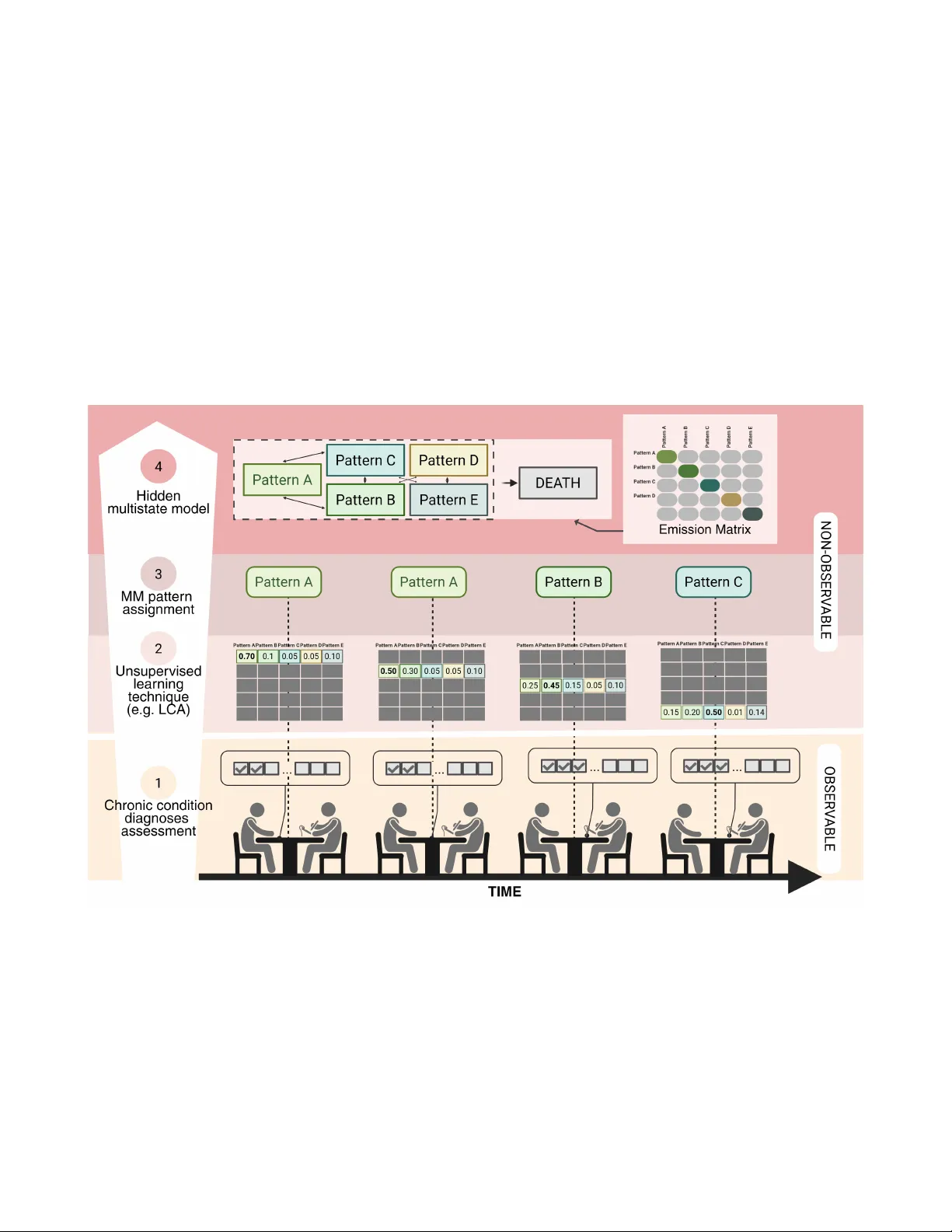
Hidden m ultistate models to study m ultimorbidity trajectories V alentina Manzoni 1 , Francesca Iev a 1,2 , Amaia Calder ´ on-Larra ˜ naga 3,4 , Davide Liborio V etrano 3,4 , and Caterina Gregorio 3* 1 MO X - modeling and Scientific Computing Laborator y , Depar tment of Mathematics, P olitecnico di Milano, Italy 2 HDS, Health Data Science center , Human T echnopole , Italy 3 Aging Research Center , Depar tment of Neurobiology , Care Sciences and Society , Karolinska Institutet and Stockholm Univ ersity , Sweden 4 Stockholm Gerontology Research Center , Stockholm, Sw eden * caterina.gregorio@ki.se ABSTRA CT Multimorbidity in older adults is common, heterogeneous, and highly dynamic, and it is strongly associated with disability and increased healthcare utilization. Howe ver , e xisting approaches to studying multimorbidity trajectories are largely descriptive or rely on discrete-time models , which struggle to handle irregular observation intervals and right-censoring. We de veloped a contin uous-time hidden multistate modeling framework to capture transitions among latent multimorbidity patterns while accounting f or inter val censoring and misclassification. A simulation study compared alternative model specifications under varying sample sizes and f ollow-up schemes , and the best-performing specification was applied to longitudinal data from the Swedish National study on Aging and Care–Kungsholmen (SNA C-K), including 2,716 multimorbid par ticipants follo wed f or up to 18 years . Simulation results show ed that hidden multistate models substantially reduced bias in tr ansition hazard estimates compared to non-hidden models, with fully time-inhomogeneous models outperforming piecewise approximations . Application to SNA C-K confir med the feasibility and pr actical utility of this framework, enab ling identification of r isk f actors for acceler ated progression tow ard complex m ultimorbidity and rev ealing a gradient of mortality r isk across patter ns. Continuous-time hidden multistate models pro vide a robust alternative to traditional approaches , suppor ting individualized predictions and inf or ming targeted inter v entions and secondar y prev ention strategies f or multimorbidity in aging populations. Introduction The global population is aging at an unprecedented rate, with projections indicating that by 2050, individuals aged 60 and ov er will outnumber younger age groups in man y regions of the world 1 . This demographic shift brings profound implications for public health, as aging is increasingly associated with comple x, dynamic, and heterogeneous health trajectories. Such patterns challenge traditional approaches that focus on single diseases, linear aging processes, or short-term clinical outcomes, and highlight the need for models capable of capturing interdependent and ev olving health changes. T o address this complexity , there is a gro wing need for adv anced statistical frame works that can represent the intrinsic heterogeneity of aging processes ov er time. These tools are essential for studying geriatric syndromes, which inherently reflect the multif actorial and systemic nature of aging. Among them, multimorbidity—defined as the co-occurrence of multiple chronic conditions 2 —has emerged as the most pre valent and impactful health issue in older adults 3 . Multimorbidity serves as a paradigmatic example of the aging process itself, capturing the cumulativ e, interacting, and individualized patterns of health decline that characterize later life. Multimorbidity has significant clinical rele vance. Among older adults, 10–15% e xperience physical frailty 4 , 20% will recei ve a diagnosis of dementia 5 , and 15–20% will become dependent in acti vities of daily li ving 6 . Multimorbidity significantly dri ves healthcare utilization, accounting for the majority of general practitioner consultations and increasing the risk of hospital admissions 7 . A defining feature of multimorbidity is that multiple diseases do not occur independently , but instead co-occur in patterns that exceed random chance 8 . These clusters can arise from shared en vironmental exposures, causal relationships between conditions, adverse effects of treatments, or common genetically determined mechanisms 9 . Since simple disease counts f ail to reflect the complexity of multimorbidity , pattern-based approaches are increasingly used to identify more homogeneous subgroups. These patterns ha ve shown predictiv e value for outcomes such as mortality 10 , 11 frailty 4 , disability , institutionalisation, and hospitalizations 10 , supporting their potential use in guiding targeted prev ention and care strategies. While pattern-based approaches hav e advanced our ability to stratify older populations and predict adverse outcomes, they remain largely static and cross-sectional. A major challenge in the field is ho w to mov e beyond these snapshots to characterize the trajectories of multimorbidity o ver time, thereby capturing its dynamic and e volving nature 12 , 13 . Understanding these trajectories is crucial for (1) identifying risk factors that driv e progression tow ard more clinically complex multimorbidity patterns, and (2) recognizing homogeneous longitudinal paths with shared prognoses and care needs 14 . Howe ver , the main barrier to generating such e vidence is the absence of tailored statistical modeling frameworks capable of addressing these longitudinal and multidimensional research questions. In the realm of longitudinal methods for studying multimorbidity , multistate modeling of fers a promising approach to capture ho w disease patterns e volv e over time 13 . These models extend survi v al analysis by allowing transitions across a set of intermediate states and an absorbing state, typically death. Howe ver , traditional multistate models often assume that these states are directly observ able, which is rarely the case in multimorbidity research, where disease patterns are latent and prone to misclassification. T o address this limitation, we propose a fle xible framework based on continuous-time Hidden Markov Models (HMMs). This approach retains the strengths of multistate models—such as handling irre gular observation times, incorporating cov ariates, and modeling time-v arying transition risks—while explicitly accounting for uncertainty in state classification. It also remains parsimonious in terms of parameter estimation, making it suitable for complex longitudinal data. W e illustrate the utility of this frame work through a simulation study that explores how dif ferent model specifications perform under v arying study designs and data conditions. Finally , we apply the methodology to real-world data from the Swedish National study on Aging and Care–K ungsholmen (SN A C-K), examining ho w socioeconomic and lifestyle factors influence transitions to more se vere multimorbidity states. This application demonstrates the practical relev ance of continuous-time HMMs as a robust tool for modeling multimorbidity trajectories in aging research. Methodology W e begin by introducing the multistate modeling framew ork in the context of chronic disease research, which serves to highlight the key challenges and distincti ve features of applying such models in this domain. W e then e xtend the framework to accommodate transitions across latent multimorbidity patterns, which represent clusters of co-occurring diseases. Figure 1 presents an ov erview of the proposed methodology and conceptual frame work, of fering a graphical summary of our approach. Multistate Modeling Framew ork A multistate model describes a stochastic process, S ( t ) , t > 0 , that records subjects’ moving across a set of discrete health states, S 15 , 16 , ov er time. S contains a number of transient states, reflecting dif ferent health-living states, and "Death" as the absorbing state, i.e. subjects cannot exit this state and transition to others. T ime is treated as a continuous v ariable, allowing transitions between states to occur at any moment—a realistic assumption when modeling medical and biological processes. Specifically , the timescale used in the multistate models considered here is the indi vidual’ s age. Consequently , each subject may hav e a different time origin in the model, corresponding to their age at study entry . In the context of aging and the development of chronic conditions, it is highly unlikely that transitions between health states are recorded at the exact moment they occur . Only acute health events typically allo w for precise timing of state changes. More commonly , indi viduals are assessed at discrete intervals—such as during routine medical visits or scheduled health surve ys—and transitions are inferred from these periodic observations. This observation mechanism results in panel data, characterized by intermittent observ ation and interval censoring: while it is known that a transition occurred between two observation points, the exact timing remains unkno wn. In addition, unlike continuous monitoring, which captures e very state transition in real time, panel data provide only snapshots of an indi vidual’ s health status at specific time points. As a result, the complete sequence of states occupied during the observ ation period is often partially observed, and some transitions may go undetected. Traditional multistate models, ho wever , assume continuous observation and precise tracking of state changes, which may not align with the realities of such data. T o address this, our work employs multistate modeling approaches specifically designed for panel data, which account for the intermittent nature of observations during parameter estimation. Importantly , we assume that observ ation times are non-informativ e—that is, the timing of measurements is independent of the underlying multistate process. Additionally , we adopt the Marko v assumption, meaning that the probability of transitioning to a future state, and the timing of that transition depend solely on the current state and the individual’ s current age: Pr [ S ( t + h ) = y | S ( r ) = s ( r ) , r ≤ t ] = Pr [ S ( t + h ) = y | S ( t ) = S ( t )] , ∀ h > 0 . (1) A multistate model is uniquely defined by a set of transition intensity functions, q i j ( t , x ) , which represent the instantaneous probability at each time t of moving between each pair of states i and j , for i , j ∈ S . In the continuous-time case, the transition intensities can be represented in a nxn matrix Q , with n total number of states, whose rows sum to zero. The K olmogorov Forward Equations (Chapman-Kolmogoro v Differential Equations) are used to describe the ev olution of probabilities over time in a Continuous T ime Multistate Models (CTMM). These equations provide a mathematical frame work to calculate the 2/ 15 probability of being in a specific state at any giv en time. Let P ( t ) represent the n × n matrix of state probabilities, where p i j ( t ) is the probability of being in state j at time t , gi ven that the process started in state i at time 0. The K olmogorov Forward Equation is giv en by: d P ( t ) d t = P ( t ) · Q (2) For each state pair ( i , j ) , the deriv ati ve d p i j ( t ) dt represents the instantaneous rate of change of the probability of being in state j at time t , starting from state i . In the context of aging and chronic diseases, the matrix, Q ( t ) , of the transition intensities needs to be allo wed to vary with time, allowing the probability of transitions across the state to v ary as the individual ages. As a result, the solution of the K olmogorov F orward Equations (KFEs) becomes more complex as it requires inte gration over time. Direct integration requires the use of numerical solv ers 17 , which can be more computationally intensi ve and time-consuming. Alternativ ely , a numerical approximation that uses a piece wise constant version of the Q ( t ) matrix can be used to simplify computations. T o approximate the solution in the time-inhomogeneous case, the time interv al [ 0 , t ] can be di vided into small subintervals [ t i , t i + 1 ] , where ∆ t = t i + 1 − t i is the step size. The transition intensity matrix Q ( t ) is approximated as piecewise constant within each interval. This leads to the following approximation of the solution: P ( t ) ≈ P ( t 0 ) · n − 1 ∏ i = 0 e ∆ t · Q ( t i ) (3) A crucial step in the modeling process in volves selecting a parametric form for the intensity function. W e adopt the proportional hazards model due to its interpretability and widespread use in clinical research. While alternative parametric families could theoretically be considered, this study focuses on the Gompertz distribution, which reflects the natural tendency of transition intensities—such as progression to greater disease burden or death—to change monotonically with age. This choice aligns with well-documented patterns in health and disease progression 18 – 20 . According to this parametric proportional-hazard model, cov ariates x associated with transition intensities are assumed to hav e a multiplicativ e effect, and each transition i → j can hav e a different set of co variate ef fects. The transition intensities take the form: h i j ( t | x ) = λ i j e α i j t + β T i j x (4) where λ i j is the baseline rate parameter in exponential form for the transition from state i to j , α i j the shape parameter for the transition from state i to j , x the vector of co variates and β ij the vector of re gression coefficients. When α < 0 , the hazard decreases ov er time, whereas α > 0 characterizes an increasing hazard with age. For α = 0 t, the Gompertz model reduces to the exponential model, i.e. a time-homogeneous model. Hidden Multistate Models for Latent Multimorbidity P atterns Multimorbidity states are conceptualized as latent constructs—unobserv able directly but inferred from a set of categorical disease indicators, denoted as Y ( t ) = ( Y 1 ( t ) , Y 2 ( t ) , . . . , Y R ( t )) , where each Y r ( t ) indicates the presence or absence of a specific chronic condition at age t . The probability that an individual belongs to a particular multimorbidity pattern, conditional on the diseases dev eloped by time t , is giv en by P ( C k ( t ) = c | Y ( t )) , where c ∈ { 1 , 2 , . . . , C } . This probability can be estimated using existing unsupervised learning techniques, such as Latent Class Analysis (LCA) or other soft-clustering methods. Based on the observed v alues y r ( t ) , an individual can be assigned to the most likely pattern using this probability , resulting in the observed state W ( t ) . Howe ver , when analyzing transitions between latent multimorbidity states, it is important to recognize that only W ( t ) is observed, not the true latent state C ( t ) . This problem can be framed as a hidden multistate model that e xtends the classical framework by explicitly modeling the generation of the observed states from the latent (hidden) ones 21 . For each indi vidual k , at observ ation time t kn , the observed states W are generated conditionally on the latent states C via an emission matrix E . This is an n × n matrix, where the entry ( i , j ) represents the probability of observing state j giv en that the hidden state is i . These probabilities can be obtained as: e i , j = P ( W ( t kn ) = j | C ( t kn ) = i ) = P ( C = i | W = j ) · N i ∑ c k = 1 P ( C = i , W = k ) · N k (5) Since exact states are unknown, subject k ’ s contribution to the likelihood 22 needs to be calculated over all possible paths of underlying states C k 1 , . . . , C kn k : 3/ 15 L k = Pr ( w k 1 , . . . , w kn k ) = Pr ( w k 1 , . . . , w kn k | C k 1 , . . . , C kn k ) Pr ( C k 1 , . . . , C kn k ) (6) Assuming that the observed states are conditionally independent gi ven the v alues of the underlying states and the Marko v property , the contribution L k can be decomposed into sums ov er each underlying state. The sum is accumulated o ver the unknown first state, the unkno wn second state, and so on until the unknown final state: L k = ∑ C k 1 . . . ∑ C kn k Pr ( W k 1 | C k 1 ) Pr ( C k 1 ) · Pr ( W k 2 | C k 2 ) Pr ( C k 2 | C k 1 ) · · · Pr ( W kn k | C kn k ) Pr ( C kn k | C kn k − 1 ) , (7) where Pr ( W kn | C kn ) is the emission probability from the hidden state C kn to the observed state W kn . The term Pr ( C k , j + 1 | C k j ) is the ( C k j , C k , j + 1 ) -th entry of the Marko v chain transition probability matrix P ( t ) , e valuated at t = t k , j + 1 − t k j . If the hidden state is death, measured without error , whose entry time is kno wn exactly , then the contribution to the lik elihood is summed ov er the unknown state at the pre vious instant before death. Figure 1. Conceptual and analytical pipeline f or modeling multimorbidity trajectories. Chronic disease diagnoses are first aggregated using Latent Class Analysis to identify multimorbidity patterns (Steps 1–2). Indi viduals are assigned pattern membership at each visit (Step 3), and transitions across latent states—including progression to death—are modeled using a continuous - time hidden multistate model that accounts for misclassification and interv al censoring (Step 4). LCA: Latent Class Analysis; MM: Multimorbidity . Created in BioRender . Simulation Study Simulation studies use pseudo-random sampling to generate data. They constitute an in v aluable tool for statistical research, particularly for the e valuation of ne w methods and for the comparison of alternative methods. By simulating data under known conditions, the data-generating mechanism is defined by the researchers, making it possible to observ e if the analysed 4/ 15 methods are able to recover such a "ground truth". In the following, we use the ADEMP structure 23 to present the details of the simulation study considered in this work. The goal of this simulation study is to 1) verify the need to consider the latent nature of the states when modeling transition among multimorbidity patterns and, 2) compare dif ferent specifications of HMMs under different scenarios (e.g. study type, sample size). Data-generating Mechanism All key simulation parameters—including the cohort’ s age range, disease prev alences, number of latent classes, types and number of simulated diseases, minimum and maximum ages at study entry , and intervals between follow-up visits—are informed by the application data. This approach is taken to ensure that the data-generating process closely reflects realistic conditions. Figure 2 presents the three main components of the data-generating process along with the four simulation scenarios considered. A detailed step-by-step description of the data generation procedure is provided in the supplementary materials. For each scenario, 100 datasets are generated. The scenarios dif fer in terms of sample size (3,000 vs. 10,000 indi viduals per dataset) and observation scheme (studies with re gular vs. irregular follo w-ups ). • D iff eren t sam ple sizes (in di vidual s pe r dat aset ): o 300 0 o 10 ,00 0 • Dra w ag e at en try, tim e in st udy . • D r aw the three baseline cova r iat e val ues. • Popula ti on St udy (PS ): 3 - 6 y ear s inte r val s be tween fo ll ow - ups . • Ir r egu la r F ol lo w - ups (I F ): fo ll ow - up di st r ib uted acco r di ng to a We ib ul l di st r ib ution. • Sim ul ate m ul ti m or bi di ty traj ect or ies acco r di ng to the m odel be lo w . • Sim ul ate preval ent an d incident di seases con di ti on ed on the la te nt st ate . P OPULATI ON COM POSI TI ON C H R ONI C DI S EAS ES G ENER AT I NG M ECH AN I SM S TUD Y DES I G N What is the c o mpo s itio n o f the po pulat io n? H o w do c hronic dise ase s de ve l o p o ve r time ? How do w e o bs e rve indi viduals? Figure 2. Overview of the data-generating mechanism used in the simulation study . The process integrates population composition, chronic disease dev elopment, and observation schemes, with scenarios varying by sample size (3,000 vs. 10,000) and follow-up structure (re gular population-based intervals vs. irregular visits). Transitions among multimorbidity states and death follow a Gompertz-based continuous-time process. It is important to note that for illustrati ve purposes, the simulation study is conducted in a simplified setting in which chronic diseases are grouped into two dif ferent multimorbidity states: multimorbidity pattern A and multimorbidity pattern B. In addition to these states, an absorbing state representing "Death" is included, with the exact time of transition to this state assumed to be kno wn. Consequently , the data-generating multistate model comprises three states: (1) Multimorbidity Pattern A, (2) Multimorbidity Pattern B, and (3) Death. The model allows for three possible transitions: from Pattern A to P attern B (T ransition 1), from Pattern A to Death (T ransition 2), and from Pattern B to Death (T ransition 3). T ransition intensities between states are modeled using a Gompertz distrib ution. Three cov ariates are included in the simulation, although only two are specified to influence the transition intensities. The hazard function for the Gompertz distribution, which go verns the transition rates, is defined as follo ws: q i j ( t ) = λ i j exp ( α i j t ) exp ( β i j . 1 x 1 + β i j . 2 x 2 ) (8) And the loglinear formulation: ln q i j ( t | x ) = ln ( λ i j ) + α i j t + β i j . 1 x 1 + β i j . 2 x 2 (9) The parameter values are reported in T able 1 according to the loglinear formulation. Prev alent conditions at baseline are simulated conditionally on the individual’ s initial multimorbidity pattern. Incident diseases are then simulated from the set of conditions not yet developed by the indi vidual, based on the state toward which 5/ 15 T ransition Rate l og ( λ ) Shape α β x 1 β x 2 β x 3 1 -14.79613 0.1556735 -0.1957039 -0.2403646 0 2 -11.90339 0.1088540 0.1405208 -0.4468561 0 3 -11.55569 0.1071397 0.1860589 -0.3101002 0 T able 1. T rue multistate model parameters from which the simulated data are generated. they are transitioning. If the next transition is to the absorbing state of death, incident diseases are simulated conditionally on the current state instead. Additionally , we assume the presence of a subset of rare diseases (with a theoretical baseline pre valence of less than 2%) that occur independently of the multimorbidity patterns. Follo wing disease simulation, study design schemes—such as population-based sampling or irregular follow-ups—are applied to mimic the data collection process in real-world longitudinal studies. As a result, disease onset is only recorded at the first follo w-up visit after the actual onset, reflecting the interval-censored nature of observ ational data. Analysis of the simulated data The following models are presented and compared in the simulation study: 1. Non-hidden multistate model with approximate Gompertz baseline ( Appr oxTIMM ). A piece-wise constant baseline hazard function is used to approximate the time-inhomogeneous Gompertz baseline. The baseline hazard function is calculated ov er a set of time points cov ering the desired age range. The shape and rate parameters are then determined using linear interpolation. The model accounts for interval-censored data, where the exact timing of a transition is unkno wn but is known to ha ve occurred within a specific time window between follo w-up visits. The model is fitted with the R package msm 22 . 2. Hidden multistate model with approximate Gompertz baseline ( A pproxTIHMM ). This model e xtends the ApproxTIMM by considering that the states are latent. The model is fitted with the msm package. 3. Non-hidden time-inhomogeneous multistate model and Gompertz baselines ( TIMM ). TIMM uses direct numerical solutions of the system of differential equations to compute the likelihood, providing a more precise and accurate representation of the transition dynamics. Howe ver , the computational demands are significantly higher due to the complexity of solving dif ferential equations numerically . It is implemented with nhm R package 24 . 4. Hidden time-inhomogeneous multistate model with Gompertz baseline ( HTIMM ). This model e xtends the TIMM by incorporating latent states. Implemented with nhm R package. Model performance is e valuated ag ainst a benchmark model (REF), which serves as a hypothetical best-case comparator . This model reflects an idealised scenario—unattainable in real-world settings—in which latent states are fully observable and exact transition times are known. The benchmark model employs a Gompertz hazard function, consistent with the specification used in the data-generating process, and is estimated using the flexsurv package 25 . The performance of the methods in estimating model parameters is e v aluated based on bias, empirical standard error , and the cov erage of confidence intervals. T o validate the data-generating mechanism of the simulation, we first ev aluated the performances of the benchmark model (REF), which assumes exact knowledge of both transition times and states. As expected, this model correctly recovers the true parameters, as illustrated in T able 2 , T able 3 , and T able 4 , confirming the v alidity of the data-generating mechanism. Furthermore, as the sample size of subjects in the datasets increases, so does the accuracy of the estimates for the benchmark model, while their bias decreases. T able 3 and T able 4 show that all model specifications adequately recovered the co variate ef fects for Transition 2 and 3 into the absorbing non-latent state (Death, state 3). Howe ver , performance measures decreased for transitions between the two states of multimorbidity (T able 2 ), where misclassification can occur due to the latent nature of the states. In these cases, the hidden Marko v models (ApproxTIHMM and TIHMM) outperformed their non-hidden counterparts (ApproxTIMM and TIMM), showing lo wer bias and higher coverage. When comparing different study designs, the irregular visits scenario (median number of follow-ups per subject: 6, interquartile range: 3-10) exhibits lower bias but also reduced coverage compared to the population-based study scenario (median number of follo w-ups per subject: 2, interquartile range: 2-3). This seemingly paradoxical outcome arises from a decrease in standard errors, while small biases persist, ultimately leading to slight undercoverage. A similar pattern can be observed when comparing scenarios with v arying sample sizes. For instance, in simulations with a lar ger number of individuals (Nsim = 10,000), model estimates show reduced co verage due to the same reduction in standard error . 6/ 15 Regarding the estimation of the baseline transition hazard parameters (shape and rate), the fully time-inhomogeneous models (TIMM and TIHMM) demonstrated better performance than those using piecewise constant approximation of the baseline. The latter showed more variability and scenario-dependent beha vior (see supplementary material), indicating that such approximations may inadequately capture the true underlying hazard dynamics in time-varying settings. Overall, simulation results indicate that the fully time-inhomogeneous model (TIHMM), which inte grates interval censoring and the latent nature of the states, is better suited to accurately modeling transitions among latent multimorbidity patterns. T able 2. Simulation study results for T ransition 1 Population-Study n=3000 n=10000 Model Estimate Bias S.E. Bias Co verage Estimate Bias S.E. Bias Cov erage β x 1 REF -0.246 -0.006 0.009 0.95 -0.243 -0.003 0.004 0.95 ApproxTIMM -0.187 0.054 0.009 0.87 -0.176 0.065 0.005 0.74 ApproxTIHMM -0.212 0.028 0.01 0.92 -0.2 0.04 0.006 0.85 TIMM -0.192 0.048 0.009 0.88 -0.182 0.058 0.005 0.77 TIHMM -0.205 0.035 0.009 0.9 -0.193 0.048 0.005 0.85 β x 2 REF -0.192 0.003 0.012 0.96 -0.197 -0.002 0.007 0.96 ApproxTIMM -0.143 0.053 0.013 0.9 -0.136 0.059 0.006 0.84 ApproxTIHMM -0.17 0.026 0.016 0.91 -0.158 0.038 0.008 0.93 TIMM -0.14 0.056 0.013 0.9 -0.134 0.062 0.006 0.84 TIHMM -0.151 0.044 0.014 0.91 -0.143 0.053 0.007 0.84 β x 3 REF -0.007 -0.007 0.008 0.97 -0.002 -0.002 0.004 0.97 ApproxTIMM -0.005 -0.005 0.009 0.97 -0.004 -0.004 0.005 0.92 ApproxTIHMM -0.007 -0.007 0.01 0.96 -0.005 -0.005 0.006 0.92 TIMM -0.005 -0.005 0.009 0.97 -0.004 -0.004 0.005 0.92 TIHMM -0.004 -0.004 0.009 0.96 -0.004 -0.004 0.006 0.92 Irregular F ollow-up n=3000 n=10000 Model Estimate Bias S.E. Bias Cov erage Estimate Bias S.E. Bias Cov erage β x 1 REF -0.246 -0.006 0.009 0.95 -0.243 -0.003 0.004 0.95 ApproxTIMM -0.183 0.058 0.008 0.87 -0.176 0.064 0.004 0.73 ApproxTIHMM -0.194 0.047 0.009 0.86 -0.188 0.052 0.005 0.81 TIMM -0.183 0.058 0.008 0.87 -0.177 0.064 0.004 0.73 TIHMM -0.189 0.051 0.009 0.86 -0.183 0.058 0.005 0.76 β x 2 REF -0.192 0.003 0.012 0.96 -0.197 -0.002 0.007 0.96 ApproxTIMM -0.14 0.056 0.012 0.89 -0.131 0.065 0.007 0.8 ApproxTIHMM -0.149 0.047 0.014 0.9 -0.14 0.056 0.007 0.85 TIMM -0.14 0.055 0.012 0.89 -0.131 0.065 0.007 0.8 TIHMM -0.147 0.048 0.013 0.91 -0.137 0.059 0.007 0.82 β x 3 REF -0.007 -0.007 0.008 0.97 -0.002 -0.002 0.004 0.97 ApproxTIMM -0.01 -0.01 0.008 0.98 -0.006 -0.006 0.005 0.95 ApproxTIHMM -0.01 -0.01 0.009 0.98 -0.009 -0.009 0.005 0.96 TIMM -0.01 -0.01 0.008 0.97 -0.006 -0.006 0.005 0.95 TIHMM -0.01 -0.01 0.008 0.98 -0.006 -0.006 0.005 0.95 7/ 15 T able 3. Simulation study results for T ransition 2 Population-Study n=3000 n=10000 Model Estimate Bias S.E. Bias Coverage Estimate Bias S.E. Bias Coverage β x 1 REF -0.462 -0.015 0.012 0.96 -0.453 -0.006 0.006 0.97 ApproxTIMM -0.475 -0.028 0.014 0.94 -0.469 -0.022 0.007 0.94 ApproxTIHMM -0.481 -0.034 0.015 0.93 -0.476 -0.029 0.007 0.94 TIMM -0.461 -0.014 0.014 0.94 -0.455 -0.008 0.007 0.95 TIHMM -0.465 -0.018 0.014 0.95 -0.458 -0.011 0.007 0.95 β x 2 REF 0.136 -0.005 0.016 0.95 0.135 -0.006 0.008 0.95 ApproxTIMM 0.127 -0.014 0.018 0.94 0.127 -0.013 0.009 0.96 ApproxTIHMM 0.125 -0.016 0.019 0.94 0.122 -0.019 0.009 0.96 TIMM 0.136 -0.005 0.018 0.94 0.135 -0.006 0.009 0.96 TIHMM 0.137 -0.004 0.019 0.94 0.134 -0.007 0.009 0.96 β x 3 REF 0.022 0.022 0.014 0.93 0.001 0.001 0.006 0.96 ApproxTIMM 0.012 0.012 0.016 0.93 0.002 0.002 0.007 0.99 ApproxTIHMM 0.011 0.011 0.017 0.92 0 0 0.008 0.98 TIMM 0.011 0.011 0.016 0.92 0.001 0.001 0.007 0.99 TIHMM 0.01 0.01 0.017 0.9 0 0 0.007 0.99 Irregular F ollow-up n=3000 n=10000 Model Estimate Bias S.E. Bias Coverage Estimate Bias S.E. Bias Coverage β x 1 REF -0.462 -0.015 0.012 0.96 -0.453 -0.006 0.006 0.97 ApproxTIMM -0.469 -0.022 0.014 0.96 -0.453 -0.006 0.008 0.95 ApproxTIHMM -0.47 -0.023 0.015 0.96 -0.458 -0.011 0.008 0.96 TIMM -0.469 -0.023 0.014 0.96 -0.453 -0.006 0.008 0.95 TIHMM -0.47 -0.023 0.014 0.97 -0.454 -0.008 0.008 0.96 β x 2 REF 0.136 -0.005 0.016 0.95 0.135 -0.006 0.008 0.95 ApproxTIMM 0.137 -0.003 0.018 0.95 0.127 -0.014 0.009 0.97 ApproxTIHMM 0.137 -0.003 0.018 0.95 0.125 -0.015 0.009 0.97 TIMM 0.137 -0.003 0.018 0.95 0.126 -0.014 0.009 0.97 TIHMM 0.138 -0.003 0.018 0.95 0.125 -0.015 0.009 0.97 β x 3 REF 0.022 0.022 0.014 0.93 0.001 0.001 0.006 0.96 ApproxTIMM 0.016 0.016 0.016 0.91 0.001 0.001 0.007 0.99 ApproxTIHMM 0.015 0.015 0.017 0.91 0.001 0.001 0.007 0.98 TIMM 0.017 0.017 0.016 0.91 0.001 0.001 0.007 0.99 TIHMM 0.015 0.015 0.017 0.91 0 0 0.007 0.98 8/ 15 T able 4. Simulation study results for T ransition 3 Population-Study n=3000 n=10000 Model Estimate Bias S.E. Bias Coverage Estimate Bias S.E. Bias Coverage β x 1 REF -0.305 0.005 0.014 0.93 -0.312 -0.002 0.007 0.96 ApproxTIMM -0.321 -0.01 0.014 0.96 -0.323 -0.013 0.007 0.97 ApproxTIHMM -0.321 -0.011 0.014 0.97 -0.325 -0.015 0.007 0.96 TIMM -0.312 -0.002 0.014 0.96 -0.316 -0.006 0.006 0.97 TIHMM -0.312 -0.002 0.014 0.97 -0.317 -0.007 0.007 0.97 β x 2 REF 0.153 -0.034 0.018 0.93 0.186 0 0.01 0.95 ApproxTIMM 0.134 -0.052 0.019 0.97 0.167 -0.019 0.009 0.98 ApproxTIHMM 0.132 -0.054 0.019 0.95 0.165 -0.021 0.01 0.97 TIMM 0.138 -0.048 0.018 0.97 0.171 -0.015 0.01 0.98 TIHMM 0.138 -0.049 0.018 0.96 0.171 -0.015 0.01 0.98 β x 3 REF -0.004 -0.004 0.015 0.95 0.006 0.006 0.008 0.93 ApproxTIMM 0.013 0.013 0.015 0.95 0.004 0.004 0.008 0.94 ApproxTIHMM 0.015 0.015 0.016 0.97 0.005 0.005 0.008 0.94 TIMM 0.013 0.013 0.015 0.95 0.004 0.004 0.008 0.93 TIHMM 0.014 0.014 0.015 0.95 0.005 0.005 0.008 0.93 Irregular F ollow-up n=3000 n=10000 Model Estimate Bias S.E. Bias Coverage Estimate Bias S.E. Bias Coverage β x 1 REF -0.305 0.005 0.014 0.93 -0.312 -0.002 0.007 0.96 ApproxTIMM -0.322 -0.012 0.014 0.95 -0.328 -0.018 0.007 0.93 ApproxTIHMM -0.323 -0.012 0.015 0.95 -0.328 -0.018 0.007 0.94 TIMM -0.322 -0.012 0.014 0.94 -0.328 -0.018 0.007 0.93 TIHMM -0.325 -0.015 0.015 0.95 -0.329 -0.019 0.007 0.93 β x 2 REF 0.153 -0.034 0.018 0.93 0.186 0 0.01 0.95 ApproxTIMM 0.143 -0.043 0.017 0.94 0.174 -0.012 0.009 0.97 ApproxTIHMM 0.141 -0.045 0.018 0.93 0.169 -0.017 0.009 0.97 TIMM 0.145 -0.041 0.018 0.93 0.175 -0.011 0.009 0.97 TIHMM 0.142 -0.044 0.018 0.93 0.175 -0.011 0.009 0.97 β x 3 REF -0.004 -0.004 0.015 0.95 0.006 0.006 0.008 0.93 ApproxTIMM 0.007 0.007 0.015 0.93 -0.001 -0.001 0.008 0.94 ApproxTIHMM 0.009 0.009 0.015 0.93 0 0 0.008 0.94 TIMM 0.007 0.007 0.015 0.92 -0.001 -0.001 0.008 0.94 TIHMM 0.008 0.008 0.015 0.93 0 0 0.008 0.94 9/ 15 Application to the SNA C-K Cohor t SN A C-K is one of the 4 sites of the Swedish National study on Aging and Care (SNA C) 26 . SN A C is a longitudinal study on the elderly population, aimed at increasing kno wledge about aging and health trends and providing a better basis for dev eloping prev entiv e measures and elder care 26 . At each follow-up, SN A C-K participants undergo a 5-hour -long comprehensive clinical and functional assessment carried out by trained physicians, nurses, and psychologists. Physicians collect information on diagnoses via physical e xamination, medical history , examination of medical charts, self-reported information, and/or proxy interviews. Clinical parameters, lab tests, drug information, and inpatient and outpatient care records are also used to identify specific conditions. Information on participants’ deaths is deriv ed from the cause of death register . All diagnoses are coded in accordance with the International Classification of Diseases, 10th revision (ICD-10) 27 . For the analyses conducted in this study , 60 chronic disease cate gories deriv ed by a clinically dri ven methodology reported in Calderón-Larrañaga et al. 11 were used. The analyses were conducted on a subset of SNA C-K data, consisting of longitudinal records collected between 2001 and 2019 from participants enrolled at the start of the study (cohort 1). Follo w-ups are carried out ev ery 6 years for participants aged 60 to 78, and ev ery 3 years for those aged 78 and older . At baseline, cohort 1 included 3,363 indi viduals. For this study , only participants with multimorbidity ( ≥ 2 chronic conditions) at the first visit were included (N = 3,268). Participants with only one recorded visit (no follo w-ups) or with missing data were excluded, resulting in a final sample of 2,716 indi viduals and a total of 9,085 observ ations. Over the 18-year follow-up period, 1,488 participants (55%) died. The mean age at death was 85 years for men (sd=8.7) and 89 years for women (sd=8.0). At baseline, women represented 63% of the total sample. Participants underwent between two and se ven visits, with a median of 3 (IQR: 2-5) follo w-ups per individual. Figure 3. Alluvial diagram of observed transitions across multimorbidity states in the SNA C-K cohort. Each stream represents an individual’ s assigned multimorbidity pattern over time (mild: light blue; complex: dark blue), with transitions to death shown in gre y . Patterns are based on posterior membership probabilities from the latent class model and illustrate increasing mov ement toward comple x multimorbidity with age. Similarly to the simulation study , an illness-death multistate model is considered, containing two patterns of multimorbidity and death. The two patterns of multimorbidity are deriv ed from Latent Class Analysis, which has been pre viously used to identify multimorbidity patterns in this population. The "mild multimorbidity" pattern presents a higher prev alence of cardiov ascular risk factors (hypertension, diabetes, dyslipidemia and obesity), asthma and sleep disorders; which have a lo wer risk of hospitalization and disability . On the other hand, the pattern denoted as"complex multimorbidity" is characterized by higher prev alence of cardiac diseases (heart failure, bradycardias conduction disease, atrial fibrillation, and anemia), dementia and sensory impairment diseases (deafness, hearing loss, blindness, and visual loss). The diseases characterizing the complex group are known to entail greater care needs and are associated with poorer physical and cognitive function. Based on this classification, individuals’ transitions across multimorbidity states are modeled using the hidden multistate model implemented in the nhm R package, which demonstrated the best performance in the simulation study . W e include in the analysis a set of 10/ 15 potential lifestyle and socio-economic risk factors that may increase the risk of transitioning tow ards the complex multimorbidity state, as well as death. Specifically , baseline cov ariates included in the multistate model are sex, lev el of education, physical activity , living alone, alcohol consumption, smoking, and manual occupation. Out of the 2,716 participants, at baseline 1,864 (69%) indi viduals are assigned to the mild multimorbidity state and 852 (31%) to the comple x multimorbidity state. The alluvial plot sho wn in Figure 3 describes ho w indi viduals in the SN A C-K cohort transition among the two multimorbidity states and death over the older age course. As participants grow older , transitions tow ard complex multimorbidity become increasingly frequent. Moreover , individuals in the complex multimorbidity state exhibit higher mortality rates than those in the mild state of the same age. Hazard ratios for the transition from mild to complex multimorbidity , as estimated by the hidden multistate model, are presented in Figure 4a . Sedentary behavior and being male are associated with a higher hazard of transitioning to complex multimorbidity . Figure 4c illustrates how these findings translate into the predicted probability of transitioning to complex multimorbidity , comparing males versus females (right panel) and sedentary versus non-sedentary behavior (left panel) from age 60, while holding other exposures at their cohort mean v alues. In both panels, the higher-risk groups exhibit a greater probability of progressing to the comple x multimorbidity state up to around age 85, after which the increasing risk of death reduces the observed dif ferences. Finally , the predicted probability of dying from the two different multimorbidity st ates is compared in Figure 4b , confirming the higher mortality associated with complex multimorbidity . Discussion In this work, we in vestigated the use of continuous-time hidden marko v models to study transitions between multimorbidity patterns. Through a comprehensiv e simulation study , we demonstrated the potential of these models across various scenarios. Additionally , by applying the model to real-world data, we illustrated its practical utility in multimorbidity research. The current literature on transitions across multimorbidity patterns primarily relies on discrete time approaches. For instance, Roso Llorach, V etrano et al. 28 employed discrete-time Hidden Markov models to in vestigate transitions between multimorbidity clusters in the SN AC K dataset. A ke y distinction from our approach is that their analysis stratified participants by baseline age group, fitting separate discrete time models for each group. Although this method captures age related heterogeneity , it prev ents the use of age as a continuous timescale and complicates interpretation, as different cluster sets may arise for the same age group at dif ferent follo w-up times. Moreover , their approach does not allo w the estimation of cov ariate effects, limiting the identification of risk profiles associated with dif ferent transition patterns. Zacarias Pons et al. 29 applied Latent T ransition Analysis (L T A) 30 to self reported multimorbidity data from the SHARE study . L T A enables modeling transitions between latent classes and incorporating cov ariates, but transition probabilities must be re-estimated for each interval, making the method less suitable for datasets with many time points or irregular follo w-ups. Importantly , in both approaches, right censoring and survi val processes cannot be modeled according to surviv al analysis standards. In contrast, the continuous-time framework proposed in this study addresses these limitations and is better suited to complex longitudinal study designs. Hidden multistate models naturally handle irregular follo w up intervals, time to death and censoring mechanisms, and allo w modeling of time v arying transition hazards. They also enable the estimation of cov ariate ef fects on transitions — a key feature for identifying risk f actors for progression within multimorbidity trajectories. Our simulation served a dual purpose: it enabled both the comparison of dif ferent model specifications and the ev aluation of the reliability of the proposed frame work. The results underscored the importance of incorporating the latent nature of the states and a fully time-inhomogeneous baseline hazard. In some scenarios, confidence-interv al coverage fell belo w nominal lev els. This likely reflects limitations of Hessian-based v ariance estimation, suggesting that bootstrap methods may provide more robust uncertainty quantification. Be yond the simulation setting, the application to the SN AC K cohort confirmed that the modeling frame work can deli ver clinically meaningful insights in real-world epidemiological settings. By integrating latent multimorbidity patterns with continuous-time transition modeling, the analysis identified relev ant sociodemographic and beha vioral factors associated with progression to comple x multimorbidity , and highlighted the marked differences in mortality risk between patterns. Although we focused on two multimorbidity states—since the aim of this paper is to demonstrate the applicability of the method rather than to pro vide novel substantiv e evi dence in the context of multimorbidity—the modeling framework is inherently flexible and capable of accommodating more than two states. This scalability will be crucial in future epidemiological studies applying this method. It is also important to note that this frame work relies on two ke y assumptions. First, a well-defined clustering or latent model must be a vailable to ensure that the states represent clinically meaningful and homogeneous multimorbidity patterns. Second, the set of states must encompass all relev ant patterns that may appear over time. Therefore, when using this methodology , it is essential to identify clinically meaningful multimorbidity patterns in a sample that is representati ve of all age groups of interest. This aligns with current recommendations in the multimorbidity trajectory literature 13 , 14 . 11/ 15 Conclusion In this work, we presented a modeling strategy that integrates latent multimorbidity patterns with continuous - time hidden multistate models to study the dynamic e volution of multimorbidity . The simulation study demonstrated that accounting for both the latent nature of the states and time - inhomogeneous transition hazards is essential for reliable inference, and the application to the SNA C - K cohort illustrated how this framew ork can yield clinically meaningful insights in real - world settings. Although moti vated by multimorbidity , the framework is broadly applicable to longitudinal processes characterized by latent constructs, irregular observation schedules, and heterogeneous progression dynamics. Many aging - related phenomena—such as cognitiv e decline, disability progression, frailty , or evolving care needs—share these features. As such, the proposed approach provides a general and v ersatile tool for modeling complex health trajectories, with the potential to support risk stratification and inform prev entiv e strategies in aging research. 12/ 15 (a) Hazard ratios with 95% confidence interv als for transitioning from mild to complex multimorbidity , estimated using the hidden multistate model. (b) Predicted probability of death from age 60 by multimorbidity state, showing higher mortality risk for individuals in the comple x state; all cov ariates were held at cohort mean values. (c) Predicted probability of progressing to complex multimorbidity from age 60, comparing males vs. females ( left panel ) and sedentary vs. non-sedentary behavior ( right panel ), with all other covariates held at cohort mean v alues. 13/ 15 Data av ailability The simulated data were generated using the code av ailable at https://github.com/ARCbiostat/SimAgingData. git , and the code used for the analysis is a vailable at https://github.com/ARCbiostat/CTHMM_multimorbidity . Access to original SN A C-K data is av ailable to the research community upon approval by the SN A C-K data management and maintenance committee. Applications for accessing these data can be submitted through the website (https://www .snac-k.se/). References 1. United Nations Department of Economic and Social Aff airs, Population Division. W orld population prospects 2024: Summary of results. https://www .un.org/de velopment/desa/pd/sites/www .un.org.de velopment.desa.pd/files/undesa_pd_ 2024_wpp_2024_advance_unedited_0.pdf (2024). 2. Busija, L., Lim, K., Szoeke, C. et al. Do replicable profiles of multimorbidity exist? systematic revie w and synthesis. Eur J Epidemiol 34 , 1025–1053, DOI: 10.1007/s10654- 019- 00568- 5 (2019). 3. Barnett, K. et al. Epidemiology of multimorbidity and implications for health care, research, and medical education: a cross-sectional study . The Lancet 380 , 37–43, DOI: 10.1016/S0140- 6736(12)60240- 2 (2012). 4. T azzeo, C., Rizzuto, D., Calderón-Larrañaga, A. et al. Multimorbidity patterns and risk of frailty in older community- dwelling adults: a population-based cohort study . Age Ageing 50 , 2183–2191, DOI: 10.1093/ageing/afab138 (2021). 5. Grande, G., Marengoni, A., V etrano, D. L. et al. Multimorbidity burden and dementia risk in older adults: The role of inflammation and genetics. Alzheimer’ s & Dementia 17 , 768–776, DOI: 10.1002/alz.12237 (2021). 6. Marengoni, A., Akugizibwe, R., V etrano, D. L. et al. Patterns of multimorbidity and risk of disability in community- dwelling older persons. Aging Clin. Exp. Res. 33 , 457–462, DOI: 10.1007/s40520- 020- 01773- z (2021). 7. Romana, G. Q. et al. Healthcare use in patients with multimorbidity . Eur. J. Public Heal. 30 , 16–22, DOI: 10.1093/eurpub/ ckz118 (2020). 8. Prados-T orres, A., Calderón-Larrañaga, A., Hancco-Saavedra, J., Poblador -Plou, B. & van den Akk er , M. Multimorbidity patterns: a systematic revie w . J. Clin. Epidemiol. 67 , 254–266, DOI: https://doi.org/10.1016/j.jclinepi.2013.09.021 (2014). 9. Langenberg, C., Hingorani, A. D. & Whitty , C. J. M. Biological and functional multimorbidity—from mechanisms to management. Nat. Medicine DOI: 10.1038/s41591- 023- 02420- 6 (2023). 10. V etrano, D. L., Rizzuto, D., Calderón-Larrañaga, A. et al. Patterns of multimorbidity in older adults and their association with functional impairment, hospitalization, and mortality . J. Ger ontol. Ser. A 76 , 920–927, DOI: 10.1093/gerona/glab021 (2021). 11. Calderón-Larrañaga, A. et al. Assessing and measuring chronic multimorbidity in the older population: a proposal for its operationalization. The Journals Ger ontol. Ser. A 72 , 1417–1423, DOI: 10.1093/gerona/glw233 (2017). 12. Cezard, G., McHale, C. T ., Sulliv an, F ., Bowles, J. K. F . & Keenan, K. Studying trajectories of multimorbidity: A systematic scoping revie w of longitudinal approaches and evidence. BMJ Open 11 , DOI: 10.1136/bmjopen- 2020- 048485 (2021). 13. Nagel, C. L. et al. Recommendations on methods for assessing multimorbidity changes over time: Aligning the method to the purpose. The Journals Ger ontol. Ser. A 79 , glae122, DOI: 10.1093/gerona/glae122 (2024). 14. Calderón-Larrañaga, A. et al. Understanding changes in complex care needs over time: K ey research insights into multimorbidity trajectories. Lancet Heal. Longev. 6 , 100790, DOI: 10.1016/j.lanhl.2025.100790 (2025). Epub 2025 Nov 25. 15. Andersen, P . K. & K eiding, N. Multi-state models for ev ent history analysis. Stat. methods medical r esear ch 11 , 91–115 (2002). 16. Hougaard, P . Dependence structures. 112–127 (2000). 17. Petzold, L. R. Automatic selection of methods for solving stiff and nonstiff systems of ordinary differential equations. SIAM J. on Sci. Stat. Comput. 4 , 136–148 (1983). 18. Riggs, J. E. Longitudinal gompertzian analysis of parkinson’ s disease mortality in the u.s., 1955-1986: the dramatic increase in overall mortality since 1980 is the natural consequence of deterministic mortality dynamics. Mec h. Ageing Dev. 55 , 235–243, DOI: 10.1016/0047- 6374(90)90151- 5 (1990). 19. Zamshev a, M., Kluttig, A., Wienke, A. & K uss, O. Modeling chronic disease mortality by methods from accelerated life testing. Stat. Medicine 43 , 5273–5284, DOI: 10.1002/sim.10233 (2024). 14/ 15 20. Kuss, O., Baumert, J., Schmidt, C. & Tönnies, T . Mortality of type 2 diabetes in germany: Additional insights from gompertz models. Acta Diabetol. 61 , 765–771, DOI: 10.1007/s00592- 024- 02237- w (2024). 21. Jackson, C. H., Sharples, L. D., Thompson, S. G., Duffy , S. W . & Couto, E. Multistate marko v models for disease progression with classification error . J. R. Stat. Soc. Ser . D Stat. 52 , 193–209, DOI: 10.1111/1467- 9884.00351 (2003). 22. Jackson, C. H. Multi-state modelling with R: the msm package (2014). 23. Morris, T . P ., White, I. R. & Crowther , M. J. Using simulation studies to e valuate statistical methods. Stat. Medicine 38 , 2074–2102, DOI: 10.1002/sim.8086 (2019). 24. T itman, A. C. Non-homogeneous Mark ov and misclassification hidden Markov multi-state modelling in R (2019). 25. Jackson, C. H. flexsurv: A platform for parametric surviv al modeling in r . J. statistical softwar e 70 (2016). 26. SN A C. Swedish National Study on Aging and Care. https://snd.se/en/catalogue/dataset/ext0124- 1 . 27. W orld Health Organization. The International Classification of Diseases, 10th revision. 28. Roso-Llorach, A., V etrano, D. L., T revisan, C. et al. 12-year ev olution of multimorbidity patterns among older adults based on hidden markov models. Aging (Albany NY) DOI: 10.18632/aging.204395 (2022). 29. Zacarías-Pons, L., V ilalta-Franch, J., T urró-Garriga, O., Saez, M. & Garre-Olmo, J. Multimorbidity patterns and their related characteristics in european older adults: A longitudinal perspective. Ar ch. Ger ontol. Geriatr. 95 , 104428, DOI: 10.1016/j.archger .2021.104428 (2021). 30. Collins, L. M. & Lanza, S. T . Latent Class and Latent T ransition Analysis for the Social, Behavioral, and Health Sciences (W iley , New Y ork, 2010). Ackno wledgements W e thank the SN A C-K participants and the SNA C-K Group for their collaboration in data collection and management. F .I. acknowledges the support by MUR, grant Dipartimento di Eccellenza 2023-2027. C.G. acknowledges the support by the Loo och Hans Ostermans Stiftelse för medicinsk forskning. D.L.V . ackno wledges the support by the Swedish Research Council (project number 2021-03324), the Karolinska Institutet Strategic Research Area in Epidemiology and Biostatistics in 2021 and 2023, and the Karolinska Institutet Strategic Research Area in Neuroscience in 2025. 15/ 15