PRISM: Parallel Reward Integration with Symmetry for MORL

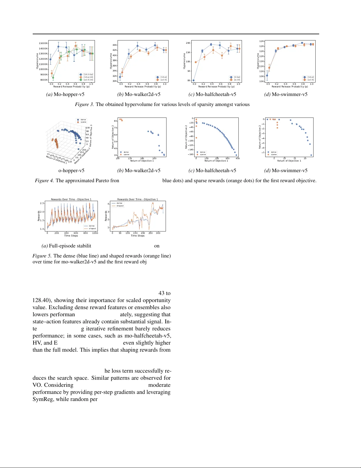
PRISM: Parallel Reward Integration with Symmetry f or MORL Finn van der Knaap 1 Kejiang Qian 1 Zheng Xu 2 Fengxiang He 1 Abstract This work studies heterogeneous Multi-Objectiv e Reinforcement Learning (MORL), where objec- tiv es can dif fer sharply in temporal frequency . Such heterogeneity allows dense objectives to dominate learning, while sparse long-horizon re- wards recei ve weak credit assignment, leading to poor sample efﬁcienc y . W e propose a Parallel Re- ward Integration with Symmetry (PRISM) algo- rithm that enforces reﬂectional symmetry as an in- ductiv e bias in aligning reward channels. PRISM introduces ReSymNet, a theory-moti vated model that reconciles temporal-frequency mismatches across objectives, using residual blocks to learn a scaled opportunity v alue that accelerates explo- ration while preserving the optimal policy . W e also propose SymReg, a reﬂectional equiv ariance regulariser that enforces agent mirroring and con- strains policy search to a reﬂection-equi variant subspace. This restriction prov ably reduces hy- pothesis complexity and impro ves generalisation. Across MuJoCo benchmarks, PRISM consistently outperforms both a sparse-reward baseline and an oracle trained with full dense rew ards, improv- ing Pareto co verage and distributional balance: it achie ves hypervolume gains exceeding 100% o ver the baseline and up to 32% over the oracle. The code is at https://github .com/EVIEHub/PRISM. 1. Introduction Reinforcement Learning (RL) has been approaching human- lev el capabilities in many decision-making tasks, such as playing Go (Silv er et al., 2017), autonomous v ehicles (Kiran et al., 2021), robotics (T ang et al., 2025a), and ﬁnance (Ham- bly et al., 2023). Multi-Objectiv e Reinforcement Learning (MORL) extends this frame work to handle multiple rew ard channels simultaneously , allo wing agents to balance com- peting objecti ves efﬁciently (Liu et al., 2014; Hayes et al., 2022). For example, a self-dri ving car must constantly bal- 1 Univ ersity of Edinburgh 2 Meta Superintelligence Labs. Corre- spondence to: Fengxiang He < F .He@ed.ac.uk > . Pr eprint. F ebruary 23, 2026. F igure 1. Reﬂectional symmetry in a two-le gged agent. The left panel shows a transition from state s to s ′ under action a , whereas the right panel shows the reﬂected transition, where states and actions are transformed by L g and K g , respectiv ely . ance multiple goals, such as minimising tra vel time while maximising passenger safety and energy efﬁciency . Pri- oritising speed would compromise the safety objectiv es, introducing the need for ﬂexible and robust policies that can optimise across div erse and sometimes conﬂicting goals. This paper considers an important, yet premature, setting where re ward channels exhibit considerable heterogeneity in facets such as sparsity . Dense objectives can o vershadow their sparse and long-horizon counterparts, steering policies tow ard short-term gains, while neglecting the objecti ves that are harder to optimise b ut potentially more important. A straightforward approach is to employ reward shaping methods to align the rew ard channels. Ho wev er, existing algorithms, such as intrinsic curiosity (P athak et al., 2017; Aubret et al., 2019) and attention-based exploration (W ei et al., 2025), are de veloped for single-objectiv e cases and hav e signiﬁcant deﬁciencies: separately shaping indi vid- ual objecti ves can distort the Pareto front and structures between objectives. This highlights a critical gap in the literature: MORL requires a re ward shaping method that en- ables efﬁcient inte gration of the parallel but heterogeneous rew ard signals, lev eraging their intrinsic structure, in order to improv e sample efﬁciency . T o this end, we propose Parallel Reward Integration with Symmetry for MORL (PRISM), a method that structurally shapes the re ward channels and lev erages the reﬂectional symmetry in agents in heterogeneous MORL problems. W e design a Rew ard Symmetry Network (ReSymNet) that pre- dicts the rew ard given the state of the system and any a vail- able performance indicators (e.g., dense rew ards in this work). The av ailable sparse re wards are used as supervised targets. In ReSymNet, residual blocks are employed to ap- proximate the ‘scaled opportunity value’, which has been 1 PRISM: Parallel Reward Integration with Symmetry f or MORL prov en to help accelerate training, decrease the approxima- tion error, while maintaining the optimal solution of the nativ e reward signals (Laud, 2004). After proper training, our ReSymNet can be a plug-and-play technique, compati- ble with an y off-the-shelf MORL algorithm in an iterativ e reﬁnement cycle, where the agent observes the shaped re- wards to impro ve its policy and the re ward model observes better trajectories from the updated policy to improv e the approximated rew ard function. T o exploit the structural information across re ward signals, we design a Symmetry Regulariser (SymRe g) to enforce reﬂectional equiv ariance of the objectives, which prov ably reduces the hypothesis complexity . Intuiti vely , incorporating reﬂectional symmetry as an inductive bias allo ws an agent to generalise experience from one situation to its mirrored counterpart. The complementary components of PRISM synergise as follo ws. Heterogeneous re ward structures cause asymmetric policy learning that violates the agent’ s physical symme- try: when dense objectives provide immediate gradients while sparse objectiv es only signal at the end of an episode, the policy may overﬁt to the denser objectiv es in speciﬁc states, failing to respect reﬂectional symmetry . ReSymNet eliminates temporal heterogeneity by aligning objectives to the same frequency , whereas SymReg enforces reﬂectional symmetry by prev enting asymmetric learning dynamics. W e prove that PRISM constrains the policy search into a subspace of reﬂection-equi variant policies. This subspace is a projection of the original polic y space, induced by the reﬂectional symmetry operator , prov ably of reduced hypoth- esis complexity , measured by covering number (Zhou, 2002) and Rademacher complexity (Bartlett & Mendelson, 2002). This reduced complexity is further translated to improved generalisation guarantees. In practice, this means that by en- couraging policies to respect natural symmetries, the agent searches ov er a smaller , more structured hypothesis space, reducing ov erﬁtting and improving sample efﬁcienc y . W e conduct extensi ve e xperiments on the MuJoCo MORL en vironments (T odorov et al., 2012; Felten et al., 2023), using Concav e-Augmented P areto Q-learning (CAPQL) (Lu et al., 2023) as the backbone for PRISM. Sparse re wards are constructed by releasing cumulati ve re wards at the end of an episode. PRISM achie ves hypervolume gains of o ver 100% against the baseline operating on sparse signals, and even up to 32% ov er the oracle (full dense re wards), also indicating a substantially improved P areto front cov erage. These gains are echoed in distrib utional metrics, conﬁrming that PRISM learns a set of policies that are also better balanced and more robust. Comprehensiv e ablation studies further conﬁrm that both ReSymNet and SymReg are critical. The code is at https://github .com/EVIEHub/PRISM. 2. Related W ork Multi-Objective Reinf orcement Lear ning. MORL algo- rithms typically fall into three cate gories: (1) single-policy methods that optimise user-speciﬁed scalarisations (Mof- faert et al., 2013; Lu et al., 2023; Hayes et al., 2022); (2) multi-policy methods that approximate the Pareto front by solving multiple scalarisations or training policies in par- allel (Roijers et al., 2015; V an Moffaert & Now ´ e, 2014; Reymond & No w ´ e, 2019; Lautenbacher et al., 2025); and (3) meta-policy and single uni versal policy methods that learn adaptable policies gi ven some preferences (Chen et al., 2019; Y ang et al., 2019; Basaklar et al., 2023; Mu et al., 2025; Liu et al., 2025). While these works hav e advanced Pareto-optimal learning, less attention has been given to heterogeneity in rew ard structures. Reward Shaping. A large volume of literature tackles sparse re wards through rew ard shaping. Potential-based shaping (Ng et al., 1999) ensures policy in variance but re- quires hand-crafted potentials. Howe ver , this method’ s re- liance on a manually designed potential function proved limiting. Intrinsic motiv ation methods reward nov elty or exploration (P athak et al., 2017; Burda et al., 2019), while self-supervised methods predict extrinsic returns from trajec- tories (Memarian et al., 2021; Devidze et al., 2022; Holmes & Chi, 2025). Recent advances utilise statistical decom- position to address sparsity (Gangwani et al., 2020; Ren et al., 2022), or capture complex re ward dependencies using transformers (T ang et al., 2024; 2025b). These approaches improv e sample efﬁciency in single-objecti ve RL, but do not extend naturally to MORL, where heterogeneous sparsity and scale can distort learning dynamics and Pareto-optimal trade-offs. Reﬂectional Equivariance. T o incorporate reﬂectional symmetry , a possible method is data augmentation, which adds mirrored transitions to the replay buf fer but doesn’t guarantee a symmetric policy and increases data process- ing costs (Lin et al., 2020). Mondal et al. (2022) propose latent space learning that encourages a symmetric represen- tation through specialised loss functions. Another line of research focuses on equi variant neural networks (van der Pol et al., 2020; Mondal et al., 2020; W ang et al., 2021). For e xample, W ang et al. (2022) design a stronger induc- tiv e bias via architecture-lev el symmetry , which hard-codes equiv ariance into the model for instantaneous generalisation. Howe ver , Park et al. (2025) show that strictly equi variant architectures can be too rigid for tasks where symmetries are approximate rather than perfect. Building on this insight, our framew ork helps overcome the limitations of strictly equiv ariant architectures through tunable ﬂe xibility whilst being model-agnostic. 2 PRISM: Parallel Reward Integration with Symmetry f or MORL 3. Preliminaries Multi-Objective Markov Decision Process. Formally , we deﬁne an MORL problem via the Multi-Objective Markov Decision Process (MOMDP) model, as a tuple M = ( S , A , P , r , γ ) : an agent at state s from a ﬁnite or continuous state space S , taking action a from a ﬁnite or continuous action space A , moves herself according to a transition probability function P : S × A × S ′ → [0 , 1] , also denoted as P ( s ′ | s, a ) . The agent recei ves a re ward via an L - dimensional vector-v alued reward function r : S ×A → R L , where L is the reward channel number , which decays by a discount factor γ ∈ [0 , 1) . The goal in MORL is to ﬁnd a policy π : S → A that optimises the expected cumula- tiv e vector return, deﬁned as J ( π ) = E π [ P ∞ t =0 γ t r t ] . This paper addresses episodic tasks, where each interaction se- quence has a ﬁnite horizon and concludes when the agent reaches a terminal state, at which point the en vironment is reset. Episodes τ i are i.i.d. draws from the behaviour distribution D , which describes the probability of observ- ing dif ferent possible trajectories under the policy being followed. Reward Sparsity . Reward sparsity can be modelled as releasing the cumulative rew ard accumulated since the last non-zero re ward with probability p rel at each timestep. When p rel = 0 , this reduces to the most extreme case: the agent receives rewards from dense channels D C = { d 1 , d 2 , . . . , d D } with observ able re wards r d i t at e very timestep, but the sparse channel is rev ealed only once at the end of the episode as R sp T = P T t =1 r sp t . The central challenge is to recover instantaneous sparse rew ards r sp t for each ( s t , a t ) using only the cumulati ve observ ation R sp T and correlations with dense channels. Formally , giv en a trajec- tory τ = { ( s 1 , a 1 ) , . . . , ( s T , a T ) } with cumulati ve sparse rew ard R sp ( τ ) , the task is to infer r sp = [ r sp 1 , . . . , r sp T ] ⊤ , where r sp t is the sparse rew ard at timestep t , such that P T t =1 r sp t ≈ R sp ( τ ) . For p rel > 0 , an episode decomposes into sub-trajectories where the same formulation applies. Generalisability and Hypothesis Complexity . A generali- sation gap, at the episodic le vel, characterises the generalis- ability from a good empirical performance to its expected performance on ne w data (W ang et al., 2019). It depends on the hypothesis set’ s complexity , which is measured in this work by cov ering number (Zhou, 2002) and Rademacher complexity (Bartlett & Mendelson, 2002). Deﬁnition 3.1 ( l ∞ , 1 distance) . Let X be a feature space and F a space of functions from X to R n . The l ∞ , 1 - distance on the space F is deﬁned as l ∞ , 1 ( f , g ) = max x ∈X ( P n i =1 | f i ( x ) − g i ( x ) | ) . Deﬁnition 3.2 (cov ering number) . The covering number, denoted N ∞ , 1 ( F , r ) , is the minimum number of balls of radius r required to completely cov er the function space F under the l ∞ , 1 -distance. Deﬁnition 3.3 (Rademacher complexity) . Let F be a class of real-valued functions on a feature space X , and let τ 1 , . . . , τ N be i.i.d. samples from a distribution over X . The empirical Rademacher complexity of F is ˆ R N ( F ) = E σ [sup f ∈F 1 N P N i =1 σ i f ( τ i )] , where σ 1 , . . . , σ N are inde- pendent Rademacher random v ariables taking v alues ± 1 with equal probability . The Rademacher complexity of F is the expectation o ver the sample set. 4. Parallel Reward Integration with Symmetry This section introduces our algorithm PRISM. 4.1. ReSymNet: Reward Symmetry Network T o address the challenge of heterogeneous reward objecti ves, PRISM ﬁrst transforms sparse re wards into dense, per-step signals. W e frame this as a supervised learning problem, inspired by but distinct from in verse reinforcement learning, as we do not assume access to expert demonstrations (Ng & Russell, 2000; Arora & Doshi, 2021). The goal is to train a rew ard model, R pred , parametrised by ψ , that learns to map state-action pairs to individual e xtrinsic rewards. W e hope to train the reward shaping model on a dataset col- lected by ex ecuting a purely random polic y , ensuring broad state-space co verage. For each timestep t , we construct a feature vector h t = [ s t , a t , r dense t ] , where s t is the state, a t is the action, and r dense ,t are the dense rewards obtained from taking action a t at state s t , which crucially le verages the information from already-dense objecti ves to help pre- dict the sparse ones. Figure 2 visualises the ResNet-like architecture. Remark 4.1 . Residual connections in R pred are inspired by the theory of scaled opportunity value (Laud, 2004), whose additiv e corrections preserve optimal policies, shorten the effecti ve re ward horizon, and improv e local value approxi- mation (see Appendix B). The network is optimised by minimising the mean squared error between the sum of its per-step predictions over a trajectory and the true cumulati ve sparse re ward observed for that trajectory: L ( ψ ) = X τ ∈D X t ∈ τ R pred ( h t ; ψ ) − R sp ( τ ) ! 2 . (1) T o ensure the learned re ward function is rob ust and adapts to the agent’ s improving policy , we incorporate two tech- niques: (1) we train an ensemble of re ward models to reduce variance and produce a more stable shaping signal, and (2) we employ iterati ve reﬁnement: the rew ard model is pe- riodically updated using new , on-policy data collected by the agent. This allows the rew ard model to correct for the initial distribution shift and remain accurate as the agent’ s 3 PRISM: Parallel Reward Integration with Symmetry f or MORL F igure 2. Overvie w of ReSymNet. behaviour e volv es from random exploration to e xpert execu- tion, as outlined in Algorithm 1 in Appendix B. 4.2. SymReg: Enforcing Reﬂectional Equi variance Howe ver , aligning re ward frequencies alone is insufﬁcient, as heterogeneous re wards cause the policy to learn asym- metrically across objecti ves, violating the agent’ s physical symmetry . T o address this, we lev erage reﬂectional sym- metry as an inductiv e bias to prev ent asymmetric policy learning. For example, for legged agents, ﬂexing a leg is essentially the mirror image of extending it. Standard poli- cies must learn both motions separately , wasting data. By encoding symmetry as an inductive bias, e xperience from one motion can be reused for its mirror , improving sample efﬁcienc y and robustness. W e formalise this physical intuition using group theory , speciﬁcally the reﬂection group G = Z 2 . This group consists of two transformations: the identity and a nega- tion/reﬂection operator , g . Let S ⊆ R d s and A ⊆ R d a denote the state and action spaces, respectively , where d s is the dimension of the state space and d a of the ac- tion space. W e deﬁne index sets I s asym ⊂ { 1 , . . . , d s } and I s sym ⊂ { 1 , . . . , d s } such that I s asym ∩ I s sym = ∅ and I s asym ∪ I s sym = { 1 , . . . , d s } . This partitions the state vector as s = ( s asym , s sym ) where s asym = s I s asym and s sym = s I s sym . W e ﬁrst partition the state vector s into an asymmetric part, s asym (e.g., the torso’ s position), and a symmetric part, s sym (e.g., the leg’ s relati ve joint angles and v elocities in Figure 1). The state transformation operator , L g : S → S , reﬂects the sym- metric part of the state as follo ws: L g ( s ) = ( s asym , − s sym ) . Similarly , we deﬁne index sets I a asym and I a sym for the ac- tion space, and the action space is split up into an asym- metric part, a asym , and a symmetric part, a sym . The ac- tion transformation operator , K g : A → A , reﬂects the symmetric part of the action (e.g., the leg torques): K g ( a ) = ( a asym , − a sym ) . The goal is to learn a policy , π , that is equiv ariant in terms of the aforementioned transformation. A policy π is reﬂectional-equiv ariant if it satisﬁes the following con- dition for all states s ∈ S : π ( L g ( s )) = K g ( π ( s )) . This property means that the action for a reﬂected state is the same as the reﬂection of the action for the original state. T o enforce this, we introduce a Symmetry Regulariser (Sym- Reg) that explicitly penalises deviations from the desired symmetry property . During training, for each observ ation s , we compute both the standard policy output π ( a | s ; ϕ ) , parameterised by ϕ , and the output for the reﬂected state π ( a | L g ( s ); ϕ ) . The equiv ariance loss is then deﬁned as: L eq = E s ∼D ,a ∼ π ϕ  ∥ π ( a | L g ( s ); ϕ ) − K g ( π ( a | s ; ϕ )) ∥ 2 1  . SymReg measures the de viation between the policy’ s actual response to a reﬂected state and the expected reﬂected re- sponse. The training objecti ve combines the standard policy gradient loss, J π ( ϕ ) , with SymReg: L total = J π ( ϕ ) + λ L eq , where λ is a hyperparameter controlling SymReg. 5. Theoretical Analysis This section presents theoretical guarantees of PRISM’ s gen- eralisability . Let Π be the full hypothesis space of policies represented by ReSymNet, R ( π ; τ ) is the cumulativ e return for a single trajectory τ obtained following polic y π . Remark 5.1 . As the backbone of the whole method, the hypothesis complexity and generalisability of ReSymNet contribute signiﬁcantly to the generalisability of the whole algorithm. Due to space limit, we present Theorem B.8 in the appendices for the cov ering number of ReSymNet’ s hypothesis space. The theory relies on these assumptions: Assumption 5.2 (bounded returns) . For all policies π and trajectories τ , 0 ≤ R ( π ; τ ) ≤ B . Assumption 5.3 (Lipschitz-continuous return) . There e xists L R > 0 such that for all π , ˜ π ∈ Π and any trajectory τ , | R ( π ; τ ) − R ( ˜ π ; τ ) | ≤ L R d ( π , ˜ π ) , where d ( π , ˜ π ) := sup s ∈S ∥ π ( s ) − ˜ π ( s ) ∥ 1 . Assumption 5.4 (compact spaces) . The state space S and action space A are compact metric spaces. Assumption 5.5 (bounded policy) . Policies π ∈ Π hav e bounded inputs and weights. Assumption 5.6 (episode sampling) . The behaviour distri- bution D has state marginal lower -bounded by p min > 0 4 PRISM: Parallel Reward Integration with Symmetry f or MORL on the state support of interest (ﬁnite-support or density lower -bound assumption). The Assumptions are reasonably mild. (Bartlett et al., 2017) prov e that feedforward ReLU are Lipschitz functions; since our policies are implemented as ReLU networks, this en- sures bounded sensiti vity of the policy outputs to perturba- tions. Assuming further that the return function is Lipschitz in the policy outputs, it follo ws that returns are Lipschitz in the policies themselves, as stated in Assumption 5.3. As- sumption 5.6 ensures that all relev ant states are sufﬁciently sampled under the behaviour policy , which is, in practice, reasonable because policy exploration mechanisms pre vent the policy from collapsing onto a subset of states. 5.1. Generalisability of Reﬂection-Equivariant Subspace Let G = Z 2 act on states and actions via L g , K g . An orbit- av eraging operator Q ( π )( s ) = 1 2  π ( s ) + K g ( π ( L g ( s )))  maps any policy to a reﬂection-equi variant subspace (Qin et al., 2022). The regulariser L eq = E s ∥ π ( L g ( s )) − K g ( π ( s )) ∥ 2 1 encourages con vergence to the ﬁxed-point sub- space, deﬁned as follows. Deﬁnition 5.7 (reﬂection-equiv ariant subspace) . W e deﬁne reﬂection-equiv ariant subspace as Π eq := { π : π ( L g ( s )) = K g ( π ( s )) } . W e pro ve that Q is reﬂectional equiv ariant, a projection, and that its image coincides with the set of equi variant policies in Lemmas C.4, C.5, and C.6 in Appendix C.3, respectiv ely . Thus, Q is surjecti ve onto Π eq . T o prove that the subspace Π eq is less complex, we show that the projection Q is non- expansi ve, which implies its image has a covering number no larger than the original space. Theorem 5.8. The space Π eq has a covering number less than or equal to that of Π . Let N ∞ , 1 ( F , r ) be the covering number of a function space F under the l ∞ , 1 -distance. Then, N ∞ , 1 (Π eq , r ) ≤ N ∞ , 1 (Π , r ) . The l ∞ , 1 -distance between two policies π ϕ and π θ is d ( π ϕ , π θ ) = sup s ∥ π ϕ ( s ) − π θ ( s ) ∥ 1 . The distance between their projections, d ( Q ( π ϕ ) , Q ( π θ )) , is no larger using the fact that K g is a norm-preserving isometry , ∥ K g ( a ) ∥ 1 = ∥ a ∥ 1 , and that L g is a bijection, which implies that the supremum ov er s equals the supremum ov er L g ( s ) . Hence Q is non-expansi ve, and a non-expansi ve surjectiv e map cannot increase the covering number . Following Lemma C.6, N (Π eq , r ) ≤ N (Π , r ) . A detailed proof can be found in Appendix C.4. The symmetrisation technique is fundamental in empiri- cal process theory that reduces the problem of bounding uniform deviations to analysing Rademacher complexity (Bartlett & Mendelson, 2002). Corollary 5.9. F or any class F of functions bounded in [0 , B ] , the expected supr emum of empirical deviations satis- ﬁes: E " sup f ∈F      1 N N X i =1 ( f ( τ i ) − E [ f ])      # ≤ 2 E [ R N ( F )] , wher e R N ( F ) = E σ h sup f ∈F 1 N P N i =1 σ i f ( τ i ) i is the Rademacher complexity and σ i ar e independent Rademacher r andom variables taking values ± 1 . This bound transforms the original centred empirical process into a symmetrised version that is often easier to analyse. W e now prove a high-probability uniform generalisation bound ov er the reﬂection-equiv ariant subspace. A detailed proof can be found in Appendix C.5. W e recognise that PRISM does not necessarily con verge to it, which will be discussed in the following subsection. Theorem 5.10. W ith R Π eq = { τ 7→ R ( π ; τ ) : π ∈ Π eq } , ﬁx any accuracy par ameter r ∈ (0 , B ) and conﬁdence δ ∈ (0 , 1) . Then with pr obability at least 1 − δ , sup π ∈ Π eq | J ( π ) − ˆ J N ( π ) | ≤ C Z B r r log N ∞ , 1 ( R Π eq , ε ) N dε ! + 8 r √ N + B r log(2 /δ ) 2 N , wher e C is an absolute numeric constant, J ( π ) is the pop- ulation expected r eturn and ˆ J N ( π ) = 1 N P N i =1 R ( π ; τ i ) is the empirical r eturn on N i.i.d. episodes τ 1 , . . . , τ N . Corollary 5.11. Under the same assumptions as Theo- r em 5.10, for any r ∈ (0 , B ) and δ ∈ (0 , 1) , the upper bound in Theor em 5.10 for Π eq is at most the same bound obtained by r eplacing Π eq with Π . By Lemma C.8, the r eturn-class covering numbers can be bounded by those of the policy class with radius scaled by 1 /L R . Mathemati- cally , following Theorem 5.8, for e very ε > 0 , log N ∞ , 1  Π eq , ε/L R  ≤ log N ∞ , 1  Π , ε/L R  , (2) hence the upper bound in Theor em 5.10 is no lar ger when evaluated on Π eq . The equi variance re gulariser projects policies onto a smaller ﬁxed-point subspace Π eq , which prov ably has cov ering num- bers no lar ger than Π . The return class inherits this reduction via the Lipschitz map, so the Dudley entropy integral for Π eq is bounded by that of Π . As such, the upper bound on the generalisation gap is no larger for Π eq compared to Π . 5.2. Generalisability of PRISM W e now study the generalisability of PRISM, which does not necessarily con verge to the reﬂection-equiv ariant subspace 5 PRISM: Parallel Reward Integration with Symmetry f or MORL exactly . Rather , PRISM might con verge to an approximately reﬂection-equiv ariant class. Using the orbit averaging Q , we quantify this effect belo w . Deﬁnition 5.12 (approximately reﬂection-equi variant class) . Approximately reﬂection-equiv ariant class is deﬁned as Π approx ( ε eq ) := { π ∈ Π : L eq ≤ ε eq } . Theorem 5.13. Let ξ := 1 2 p ε eq /p min . Then for every policy π ∈ Π , | J ( π ) − J ( Q ( π )) | ≤ L R · d ( π , Q ( π )) ≤ L R ξ . (3) Then every π ∈ Π approx ( ε eq ) lies in the sup-ball of r adius ξ ar ound Π eq . Consequently , for any tar get covering radius r > ξ , we have: N ∞ , 1  Π approx ( ε eq ) , r  ≤ N ∞ , 1  Π eq , r − ξ  . (4) By Lipschitzness of returns, the expected return of a policy and its projection dif fer by at most L R d ( π , Q ( π )) . The mis- match ∆ π controls this distance, and Lemma C.10 bounds its supremum by ξ , giving the ﬁrst inequality . Geometrically , Π approx ( ε eq ) is contained in a ξ -tube around Π eq . Hence any ( r − ξ ) -cov er of Π eq yields an r -cov er of Π approx ( ε eq ) , proving the co vering-number relation (see Appendix C.6 for a detailed proof). Theorem 5.14. W ith R Π eq = { τ 7→ R ( π ; τ ) : π ∈ Π eq } , ﬁx any accuracy par ameter r ∈ (0 , B ) and conﬁdence δ ∈ (0 , 1) . Then with pr obability at least 1 − δ , sup π ∈ Π approx ( ε eq ) | J ( π ) − ˆ J N ( π ) | ≤ C Z B r r log N ∞ , 1 ( R Π eq , ε ) N dε ! + 8 r √ N + B r log(2 /δ ) 2 N + 2 L R ξ . For π ∈ Π approx ( ε eq ) , decompose the generalisation er- ror relative to its projection Q ( π ) ∈ Π eq . The dif ferences in population returns | J ( π ) − J ( Q ( π )) | and in empirical returns | ˆ J N ( π ) − ˆ J N ( Q ( π )) | are bounded by L R ξ (Theo- rem 5.13). The middle term | J ( Q ( π )) − ˆ J N ( Q ( π )) | is the generalisation error of an equi variant polic y . T aking supre- mum, an equi variant bound is obtained (Theorem 5.10) plus 2 L R ξ . Detailed proofs are in Appendix C.6. Corollary 5.15. Under the same assumptions as Theo- r em 5.14, for any r ∈ (0 , B ) and δ ∈ (0 , 1) , the upper bound in Theorem 5.14 for Π approx ( ε eq ) is at most the same bound obtained by replacing Π approx ( ε eq ) with Π . By Lemma C.8, the r eturn-class covering numbers can be bounded by those of the policy class with radius scaled by 1 /L R . F or any tar get covering r adius r > ξ , we have log N ∞ , 1  Π approx ( ε eq ) , r /L R  ≤ log N ∞ , 1  Π eq , ( r − ξ ) /L R  ≤ log N ∞ , 1  Π , ( r − ξ ) /L R  . (5) Hence the upper bound in Theor em 5.14 is no lar ger when evaluated on Π eq . The cov ering relation incurs a slack of size ξ , leading to bounds of the form N (Π approx ( ε eq ) , r ) ≤ N (Π eq , r − ξ ) ≤ N (Π , r − ξ ) . By contrast, in Corollary 5.11, this slack disappears. Thus, the exact case guarantees a strict reduction in complexity , whereas the approximate case trades a ξ - shift in the radius for retaining proximity to the equiv ariant subspace. 6. Experiments W e conduct extensi ve experiments to verify PRISM. The code is at https://github .com/EVIEHub/PRISM. 6.1. Experimental Settings En vironments. Four MuJoCo (T odoro v et al., 2012) en vi- ronments are used: mo-hopper-v5, mo-walker2d-v5, mo- halfcheetah-v5, and mo-swimmer-v5. T able 3 in Appendix D displays the environments and their dimensions, high- lighting the div ersity in space complexity . As a result, a method must be able to ﬁnd general solutions applicable to various MORL challenges, instead of being just tailored to one speciﬁc type of problem. Furthermore, the di vision of asymmetric and symmetric state and action spaces to model equiv ariance is detailed in Appendix D. Baselines. PRISM is adaptable to any of f-the-shelf MORL algorithm. In this work, CAPQL (Lu et al., 2023) is used as a backbone model, which is a method that trains a sin- gle univ ersal network to cov er the entire preference space and approximate the Pareto front. W e produce (1) oracle: instead of artiﬁcially setting a re ward channel to be sparse, this baseline model can be seen as the gold standard, and (2) baseline: instead of utilising the proposed rew ard shaping model, this method uses CAPQL (Lu et al., 2023) and only observes the sparse re wards. Evaluation. W e use hypervolume (HV), Expected Utility Metric (EUM), and one distributional metric, V ariance Ob- jectiv e (VO) (Cai et al., 2023), for e valuation. The used hyperparameters, together with a detailed explanation of ev aluation metrics, can be found in Appendix E. 6.2. Empirical Results Reward Sparsity Sensitivity . Figure 3 illustrates the sensi- tivity of MORL agents to varying le vels of re ward sparsity . 6 PRISM: Parallel Reward Integration with Symmetry f or MORL Across all en vironments, we observe a sharp decline in HV when one objective is made extremely sparse, with reduc- tions ranging from 20 to 40% relati ve to the dense setting. These results conﬁrm that sparse objecti ves w orsen policy quality , as agents tend to neglect long-term sparse signals in fav our of denser objecti ves. For the rest of the paper , we continue with the most dif ﬁcult setting where extreme sparsity is imposed on the ﬁrst rew ard objective. Return Distrib ution of Policy . Figure 4 illustrates the im- pact of mixed sparsity on MORL across the considered en vi- ronments. Each subplot compares the approximated Pareto fronts obtained when objectiv e one is dense (blue dots) ver- sus when it is made sparse (orange dots), while keeping all other objectiv es dense. Extreme sparsity is imposed, where the sparse reward is released at the end of an episode. The results demonstrate a consistent pattern across all en- vironments: when objectiv e one becomes sparse, agents systematically fail to discover high-performing solutions along this dimension, instead concentrating their learning efforts on the remaining dense objecti ves. Comparison Experiments. T able 1 reports the obtained results for HV , EUM, and V O. The results are av eraged ov er 10 trials, with the standard deviations sho wn in grey . PRISM consistently outperforms both the oracle and base- line across environments. For mo-hopper -v5, PRISM im- prov es hypervolume by 21.5% o ver the oracle ( 1 . 58 × 10 7 compared to 1 . 30 × 10 7 ) and 88% ov er the baseline. Simi- lar gains are observ ed for mo-walker2d-v5, where PRISM achiev es a 13% HV improvement over oracle and 43% ov er the baseline. Notably , in mo-halfcheetah-v5, PRISM yields a 32% improv ement in HV compared to the oracle ( 2 . 25 × 10 4 against 1 . 70 × 10 4 ) and more than doubles the sparse result. These improvements imply that PRISM not only restores solutions lost under sparsity but also e xpands the range of trade-offs accessible to the agent. Improv e- ments in EUM follo w the same trend, with increases of up to 50% compared to the baseline. The concurrent increase in EUM demonstrates that these solutions pro vide higher expected utility , conﬁrming that PRISM learns policies that are both div erse and practically useful. On distributional metrics, PRISM deli vers more consistent performance than both the oracle and baseline. V O in mo- hopper-v5 increases from 43.36 (baseline) and 59.07 (or- acle) to 66.66 under PRISM, and mo-walk er2d-v5 shows a 51% gain over the baseline. These gains are crucial be- cause they indicate that PRISM does not simply maximise HV by focusing on extreme solutions, b ut also produces Pareto fronts that are better balanced, rob ust, and fair across objectiv es. Figure 6 in Appendix F, which shows the ap- proximated Pareto fronts, aligns with these results. W e provide two distinct e xamples to analyse the behaviour T able 1. Experimental results. W e report the a verage hypervolume (HV), Expected Utility Metric (EUM), and V ariance Objecti ve (V O) over 10 trials, with the standard error shown in grey . The largest (best) values are in bold font. Environment Metric Oracle Baseline PRISM Mo-hopper-v5 HV ( × 10 7 ) 1.30 ± 0.13 0.84 ± 0.05 1.58 ± 0.05 EUM 129.04 ± 7.96 97.64 ± 4.18 147.43 ± 2.61 VO 59.07 ± 3.45 43.36 ± 1.61 66.66 ± 1.40 Mo-walker2d-v5 HV ( × 10 4 ) 4.21 ± 0.11 3.34 ± 0.16 4.77 ± 0.07 EUM 107.58 ± 2.86 82.13 ± 4.34 120.43 ± 1.64 VO 53.22 ± 1.39 39.18 ± 2.49 59.35 ± 0.80 Mo-halfcheetah-v5 HV ( × 10 4 ) 1.70 ± 0.20 0.97 ± 0.00 2.25 ± 0.18 EUM 81.29 ± 21.85 -1.46 ± 0.27 89.94 ± 15.33 VO 36.84 ± 10.06 -1.01 ± 0.20 40.72 ± 7.02 Mo-swimmer-v5 HV ( × 10 4 ) 1.21 ± 0.00 1.09 ± 0.02 1.21 ± 0.00 EUM 9.41 ± 0.12 4.10 ± 0.80 9.44 ± 0.14 VO 4.22 ± 0.08 1.58 ± 0.40 4.24 ± 0.07 of the learned re ward signals compared to the oracle for mo- walker2d-v5. Figure 5a illustrates a full 1000-step episode. The shaped reward is highly correlated with the dense re- ward throughout the entire trajectory . The alignment of peaks and troughs conﬁrms that ReSymNet captures the dynamics of the en vironment, ensuring accurate credit as- signment without temporal drift. Figure 5b highlights a key theoretical adv antage of ReSym- Net. In high-performance re gions (e.g., steps 250–270), the shaped reward ampliﬁes the signal, e xceeding the magnitude of the oracle. By creating steeper gradients for desirable behaviours, the shaped re ward can provide more ef fectiv e guidance than the raw en vironmental signal, explaining why PRISM is capable of outperforming the oracle. Ablation Study . W e analyse the following ablation models (w/o is the abbreviation for without), which remove sev- eral aspects of the re ward shaping model or the equi variance loss: (1) PRISM: This is the proposed method, in volving all components, (2) w/o residual: This ablation model remo ves the two residual blocks from the rew ard shaping model, (3) w/o dense rewards: W e remove the dense re wards as input features to the re ward model, (4) w/o ensemble: W e remove the ensemble of reward shaping models, and only employ one, (5) w/o r eﬁnement: Rather than updating the re ward shaping model with expert trajectories, this approach merely trains the reward shaping model using the random trajec- tories collected at ﬁrst, and (6) w/o loss: W e remov e the equiv ariance loss term and merely use the re ward shaping model. W e also include two ablation studies that remove ReSymNet from PRISM and replace the reward shaping model as follows: (7) uniform : Distributes the episodic sparse rew ard R sp ( τ ) equally across all T timesteps, and (8) random : Samples random weights α t ∼ U ( − 1 , 1) for each timestep, normalises to sum to one, and scales by the total rew ard. The ablation results in T ables 10 and 11 in Appendix G high- light the contribution of indi vidual components. Removing 7 PRISM: Parallel Reward Integration with Symmetry f or MORL 0.0 0.2 0.4 0.6 0.8 1.0 R ewar d R elease P r obability (p) 8000K 9000K 10000K 11000K 12000K 13000K 14000K 15000K Hypervolume [1.0,1.0,p] [1.0,p,1.0] [p,1.0,1.0] (a) Mo-hopper-v5 1.0 0.8 0.6 0.4 0.2 0.0 R ewar d R elease P r obability (p) 30K 32K 34K 36K 38K 40K 42K 44K Hypervolume [1.0,p] [p,1.0] (b) Mo-walker2d-v5 1.0 0.8 0.6 0.4 0.2 0.0 R ewar d R elease P r obability (p) 0K 5K 10K 15K 20K Hypervolume [1.0,p] [p,1.0] (c) Mo-halfcheetah-v5 1.0 0.8 0.6 0.4 0.2 0.0 R ewar d R elease P r obability (p) 10K 10K 11K 11K 11K 12K 12K 12K 12K Hypervolume [1.0,p] [p,1.0] (d) Mo-swimmer-v5 F igure 3. The obtained hypervolume for v arious lev els of sparsity amongst various dimensions. 75 100 125 150 175 200 225 R etur n of Objective 1 0 50 100 150 200 R etur n of Objective 2 0 20 40 60 80 100 R etur n of Objective 3 dense sparse (a) Mo-hopper-v5 100 120 140 160 R etur n of Objective 1 30 40 50 60 70 80 R etur n of Objective 2 dense sparse (b) Mo-walker2d-v5 0 100 200 300 400 R etur n of Objective 1 160 140 120 100 80 60 40 20 0 R etur n of Objective 2 dense sparse (c) Mo-halfcheetah-v5 5 10 15 20 R etur n of Objective 1 7 6 5 4 3 2 1 0 R etur n of Objective 2 dense sparse (d) Mo-swimmer-v5 F igure 4. The approximated Pareto front for dense re wards (blue dots) and sparse rewards (orange dots) for the ﬁrst re ward objectiv e. 0 200 400 600 800 1000 T ime Steps 1.0 1.5 2.0 2.5 R ewar ds R ewar ds Over T ime - Objective 1 dense shaped (a) Full-episode stability 0 50 100 150 200 250 300 T ime Steps 1 2 3 4 R ewar ds R ewar ds Over T ime - Objective 1 dense shaped (b) Signal optimisation F igure 5. The dense (blue line) and shaped re wards (orange line) ov er time for mo-walker2d-v5 and the ﬁrst rew ard objective. residual connections reduces HV and EUM across all en- vironments (e.g., mo-hopper-v5 EUM falls from 147.43 to 128.40), showing their importance for scaled opportunity value. Excluding dense re ward features or ensembles also lowers performance, but only moderately , suggesting that state–action features already contain substantial signal. In- terestingly , removing iterativ e reﬁnement barely reduces performance; in some cases, such as mo-halfcheetah-v5, HV , and EUM remain comparable or ev en slightly higher than the full model. This implies that shaping re wards from a broad set of random trajectories is already highly effecti ve. Removing the symmetry loss reduces performance across en vironments, indicating that the loss term successfully re- duces the search space. Similar patterns are observed for V O. Considering ReSymNet, uniform achie ves moderate performance by providing per-step gradients and le veraging SymReg, while random performs poorly due to noisy , mis- leading re wards. PRISM consistently outperforms both by learning rew ard decomposition with ReSymNet and enforc- ing structural consistency via SymReg, enabling accurate credit assignment in complex multi-objecti ve tasks. 7. Conclusion This work proposes Parallel Re ward Integration with reﬂec- tional Symmetry for Multi-objectiv e reinforcement learn- ing (PRISM), a frame work designed to tackle sample in- efﬁcienc y in heterogeneous multi-objecti ve reinforcement learning, particularly in en vironments with sparse re wards. Our approach is centred around tw o key contrib utions: (1) ReSymNet, a theory-inspired re ward model that le verages residual blocks to align reward channels by learning a re- ﬁned ‘scaled opportunity v alue’, and (2) SymReg, a no vel regulariser that enforces reﬂectional symmetry as an induc- tiv e bias in the polic y’ s action space. W e prove that PRISM restricts polic y search to a reﬂection-equi variant subspace, a projection of the original policy space with prov ably reduced hypothesis complexity; in this way , the generalisability is rigorously improved. Extensive experiments on MuJoCo benchmarks show that PRISM consistently outperforms ev en a strong oracle with full reward access in terms of a wide range of metrics, including HV , EUM, and V O. Acknowledgements K. Qian w as supported in part by the UKRI Grant EP/Y03516X/1 for the UKRI Centre for Doctoral T rain- ing in Machine Learning Systems (https://mlsystems.uk/). 8 PRISM: Parallel Reward Integration with Symmetry f or MORL References Alegre, L. N., Bazzan, A. L. C., Roijers, D. M., No w ´ e, A., and da Silv a, B. C. Sample-ef ﬁcient multi-objecti ve learn- ing via generalized policy improv ement prioritization. In 2023 International Confer ence on Autonomous Agents and Multiagent Systems (AAMAS 2023) , pp. 2003–2012. A CM, 2023. Arora, S. and Doshi, P . A surv ey of in verse reinforcement learning: Challenges, methods and progress. Artiﬁcial Intelligence , 297:103500, 2021. Aubret, A., Matignon, L., and Hassas, S. A survey on intrinsic motiv ation in reinforcement learning. arXiv pr eprint arXiv:1908.06976 , 2019. Bartlett, P . L. and Mendelson, S. Rademacher and Gaussian complexities: Risk bounds and structural results. J ournal of Machine Learning Resear ch , 3:463–482, 2002. Bartlett, P . L., Foster , D. J., and T elgarsky , M. J. Spectrally- normalized margin bounds for neural networks. Advances in neural information pr ocessing systems , 30, 2017. Basaklar , T ., Gumussoy , S., and Ogras, ¨ U. Y . PD-MORL: Preference-driv en multi-objective reinforcement learn- ing algorithm. In Eleventh International Confer ence on Learning Repr esentations (ICLR 2023) . OpenRevie w .net, 2023. Burda, Y ., Edwards, H., Storkey , A. J., and Klimov , O. Exploration by random network distillation. In 7th Inter- national Confer ence on Learning Representations (ICLR 2019) . OpenRevie w .net, 2019. Cai, X.-Q., Zhang, P ., Zhao, L., Bian, J., Sugiyama, M., and Llorens, A. Distributional Pareto-optimal multi-objecti ve reinforcement learning. In 37th International Confer ence on Neural Information Pr ocessing Systems (NIPS 2023) , volume 36, pp. 15593–15613. Curran Associates, 2023. Chen, X., Ghadirzadeh, A., Bj ¨ orkman, M., and Jensfelt, P . Meta-learning for multi-objectiv e reinforcement learn- ing. In 2019 IEEE/RSJ International Confer ence on In- telligent Robots and Systems (IR OS 2019) , pp. 977–983. IEEE, 2019. Devidze, R., Kamalaruban, P ., and Singla, A. Exploration- guided re ward shaping for reinforcement learning under sparse re wards. In 36th International Confer ence on Neu- ral Information Pr ocessing Systems (NIPS 2022) . Curran Associates, 2022. Dudley , R. M. The sizes of compact subsets of Hilbert space and continuity of Gaussian processes. J ournal of Functional Analysis , 1(3):290–330, 1967. Felten, F ., Alegre, L. N., No w ´ e, A., Bazzan, A. L. C., T albi, E., Danoy , G., and da Silva, B. C. A toolkit for reliable benchmarking and research in multi-objecti ve reinforce- ment learning. In 37th International Conference on Neu- ral Information Pr ocessing Systems (NIPS 2023) . Curran Associates, 2023. Fonseca, C. M., P aquete, L., and L ´ opez-Ib ´ a ˜ nez, M. An im- prov ed dimension-sweep algorithm for the hyperv olume indicator . In IEEE International Conference on Evolu- tionary Computation (CEC 2006) , pp. 1157–1163. IEEE, 2006. Gangwani, T ., Zhou, Y ., and Peng, J. Learning guidance re wards with trajectory-space smoothing. In 33rd Annual Confer ence on Neural Information Pr ocessing Systems 2020 (NIPS 2020 , 2020. Hambly , B., Xu, R., and Y ang, H. Recent advances in reinforcement learning in ﬁnance. Mathematical F inance , 33(3):437–503, 2023. Hayes, C. F ., R ˘ adulescu, R., Bar giacchi, E., K ¨ allstr ¨ om, J., Macfarlane, M., Re ymond, M., V erstraeten, T ., Zintgraf, L. M., Dazeley , R., Heintz, F ., et al. A practical guide to multi-objectiv e reinforcement learning and planning. Autonomous Ag ents and Multi-Agent Systems , 36(1):26, 2022. He, F ., Liu, T ., and T ao, D. Why resnet works? residuals generalize. IEEE T ransactions on Neural Networks and Learning Systems , 31(12):5349–5362, 2020. He, K., Zhang, X., Ren, S., and Sun, J. Delving deep into rectiﬁers: Surpassing human-level performance on imagenet classiﬁcation. In 2015 IEEE International Con- fer ence on Computer V ision (ICCV 2015) , pp. 1026–1034. IEEE Computer Society , 2015. Holmes, I. and Chi, M. Attention-based re ward shap- ing for sparse and delayed re wards. arXiv preprint arXiv:2505.10802 , 2025. Kiran, B. R., Sobh, I., T alpaert, V ., Mannion, P ., Al Sal- lab, A. A., Y ogamani, S., and P ´ erez, P . Deep reinforce- ment learning for autonomous dri ving: A survey . IEEE transactions on intelligent tr ansportation systems , 23(6): 4909–4926, 2021. Laud, A. D. Theory and application of re ward shaping in r einforcement learning . University of Illinois at Urbana- Champaign, 2004. Lautenbacher , T ., Rajaei, A., Barbieri, D., V iebahn, J., and Cremer , J. L. Multi-objecti ve reinforcement learn- ing for power grid topology control. arXiv preprint arXiv:2502.00040 , 2025. 9 PRISM: Parallel Reward Integration with Symmetry f or MORL Lin, Y ., Huang, J., Zimmer , M., Guan, Y ., Rojas, J., and W eng, P . In variant transform experience replay: Data augmentation for deep reinforcement learning. IEEE Robotics and Automation Letters , 5(4):6615–6622, 2020. Liu, C., Xu, X., and Hu, D. Multiobjectiv e reinforcement learning: A comprehensiv e overvie w . IEEE T ransactions on Systems, Man, and Cybernetics: Systems , 45(3):385– 398, 2014. Liu, E., W u, Y ., Huang, X., Gao, C., W ang, R., Xue, K., and Qian, C. Pareto set learning for multi-objectiv e re- inforcement learning. In AAAI Confer ence on Artiﬁcial Intelligence , pp. 18789–18797. AAAI Press, 2025. Lu, H., Herman, D., and Y u, Y . Multi-objectiv e reinforce- ment learning: Conv exity , stationarity and Pareto optimal- ity . In Eleventh International Confer ence on Learning Repr esentations (ICLR 2023) . OpenRevie w .net, 2023. McDiarmid, C. et al. On the method of bounded dif ferences. Surve ys in Combinatorics , 141(1):148–188, 1989. Memarian, F ., Goo, W ., Lioutikov , R., Niekum, S., and T opcu, U. Self-supervised online reward shaping in sparse-rew ard environments. In 2021 IEEE/RSJ Inter- national Conference on Intelligent Robots and Systems (IR OS 2021) , pp. 2369–2375. IEEE, 2021. Moff aert, K. V ., Drugan, M. M., and Now ´ e, A. Scalar - ized multi-objectiv e reinforcement learning: Novel de- sign techniques. In 2013 IEEE Symposium on Adaptive Dynamic Pr ogramming and Reinfor cement Learning (AD- PRL 2013) , pp. 191–199. IEEE, 2013. Mondal, A. K., Nair, P ., and Siddiqi, K. Group equiv- ariant deep reinforcement learning. arXiv pr eprint arXiv:2007.03437 , 2020. Mondal, A. K., Jain, V ., Siddiqi, K., and Rav anbakhsh, S. Eqr: Equi variant representations for data-efﬁcient reinforcement learning. In International Confer ence on Machine Learning (ICML 2022) , v olume 162 of PMLR , pp. 15908–15926. PMLR, 2022. Mu, N., Luan, Y ., and Jia, Q.-S. Preference-based multi- objectiv e reinforcement learning. IEEE T ransactions on Automation Science and Engineering , 2025. Ng, A. Y . and Russell, S. Algorithms for in verse reinforce- ment learning. In Seventeenth International Confer ence on Machine Learning (ICML 2000) , pp. 663–670. Mor - gan Kaufmann, 2000. Ng, A. Y ., Harada, D., and Russell, S. Polic y in variance under rew ard transformations: Theory and application to re ward shaping. In Sixteenth International Confer ence on Machine Learning (ICML 1999) , pp. 278–287. Morgan Kaufmann, 1999. Park, J. Y ., Bhatt, S., Zeng, S., W ong, L. L. S., K oppel, A., Ganesh, S., and W alters, R. Approximate equi variance in reinforcement learning. In International Confer ence on Artiﬁcial Intelligence and Statistics (AIST ATS 2025) , volume 258 of PMLR , pp. 4177–4185. PMLR, 2025. Pathak, D., Agrawal, P ., Efros, A. A., and Darrell, T . Curiosity-driv en exploration by self-supervised predic- tion. In 34th International Confer ence on Machine Learn- ing (ICML 2017) , v olume 70 of PMLR , pp. 2778–2787. PMLR, 2017. Qin, T ., He, F ., Shi, D., Huang, W ., and T ao, D. Beneﬁts of permutation-equiv ariance in auction mechanisms. 36th International Confer ence on Neural Information Pr ocess- ing Systems (NIPS 2022) , 35:18131–18142, 2022. Ren, Z., Guo, R., Zhou, Y ., and Peng, J. Learning long-term rew ard redistribution via randomized return decompo- sition. In T enth International Conference on Learning Repr esentations (ICLR 2022) . OpenRevie w .net, 2022. Reymond, M. and No w ´ e, A. Pareto-DQN: Approximating the Pareto front in complex multi-objectiv e decision prob- lems. In Adaptive and Learning Agents W orkshop (ALA 2019) , 2019. Roijers, D. M., Whiteson, S., and Oliehoek, F . A. Com- puting con vex co verage sets for faster multi-objective coordination. Journal of Artiﬁcial Intelligence Resear ch , 52:399–443, 2015. Silver , D., Schrittwieser , J., Simonyan, K., Antonoglou, I., Huang, A., Guez, A., Hubert, T ., Baker , L., Lai, M., Bolton, A., et al. Mastering the game of go without human knowledge. Nature , 550(7676):354–359, 2017. T ang, C., Abbatematteo, B., Hu, J., Chandra, R., Mart ´ ın- Mart ´ ın, R., and Stone, P . Deep reinforcement learning for robotics: A survey of real-w orld successes. In Pr oceed- ings of the AAAI Conference on Artiﬁcial Intelligence , volume 39, pp. 28694–28698, 2025a. T ang, Y ., Cai, X.-Q., Pang, J.-C., W u, Q., Ding, Y .-X., and Sugiyama, M. Beyond simple sum of delayed rewards: Non-marko vian reward modeling for reinforcement learn- ing. arXiv pr eprint arXiv:2410.20176 , 2024. T ang, Y ., Cai, X., Ding, Y ., W u, Q., Liu, G., and Sugiyama, M. Reinforcement learning from bagged rew ard. T rans- actions on Machine Learning Resear ch , 2025b. T odorov , E., Erez, T ., and T assa, Y . MuJoCo: A physics engine for model-based control. In 2012 IEEE/RSJ Inter - national Confer ence on Intelligent Robots and Systems , pp. 5026–5033. IEEE, 2012. 10 PRISM: Parallel Reward Integration with Symmetry f or MORL van der Pol, E., W orrall, D. E., van Hoof, H., Oliehoek, F . A., and W elling, M. MDP homomorphic networks: Group symmetries in reinforcement learning. In 33st Annual Confer ence on Neural Information Pr ocessing Systems (NIPS 2020) , 2020. V an Moff aert, K. and Now ´ e, A. Multi-objecti ve reinforce- ment learning using sets of Pareto dominating policies. The Journal of Mac hine Learning Resear ch , 15(1):3483– 3512, 2014. W ang, D., W alters, R., Zhu, X., and Jr ., R. P . Equi variant Q learning in spatial action spaces. In 5th Confer ence on Robot Learning , volume 164 of PMLR , pp. 1713–1723. PMLR, 2021. W ang, D., W alters, R., and Platt, R. SO(2)-equiv ariant rein- forcement learning. In T enth International Confer ence on Learning Repr esentations (ICLR 2022) . OpenRevie w .net, 2022. W ang, H., Zheng, S., Xiong, C., and Socher , R. On the gen- eralization gap in reparameterizable reinforcement learn- ing. In 36th International Confer ence on Machine Learn- ing (ICML 2019) , volume 97, pp. 6648–6658. PMLR, 2019. W ei, W ., Li, H., Zhou, S., Li, B., and Liu, X. Attention with system entropy for optimizing credit assignment in cooperativ e multi-agent reinforcement learning. IEEE T ransactions on Automation Science and Engineering , 22: 14775–14787, 2025. Y ang, R., Sun, X., and Narasimhan, K. A generalized algorithm for multi-objectiv e reinforcement learning and policy adaptation. In 33r d International Confer ence on Neural Information Pr ocessing Systems (NIPS 2019) , pp. 14610–14621. Curran Associates, 2019. Zhou, D.-X. The covering number in learning theory . Jour - nal of Complexity , 18(3):739–767, 2002. Zintgraf, L. M., Kanters, T . V ., Roijers, D. M., Oliehoek, F ., and Beau, P . Quality assessment of MORL algorithms: A utility-based approach. In 24th Annual Mac hine Learning Confer ence of Belgium and the Netherlands , 2015. 11 PRISM: Parallel Reward Integration with Symmetry f or MORL A. Notation T able 2. Notation. Symbol Description S State space A Action space P ( s ′ | s, a ) T ransition probability r ( s, a ) ∈ R L V ector-valued re ward with L objectives γ ∈ [0 , 1) Discount factor π : S → A Policy mapping J ( π ) = E π  P ∞ t =0 γ t r t  Expected cumulativ e vector return D Behaviour distribution to sample episodes from D C = { d 1 , . . . , d D } Dense rew ard channels r d i t Rew ard from dense channel d i at timestep t r sp t Sparse rew ard at timestep t τ = { ( s 1 , a 1 ) , . . . , ( s T , a T ) } T rajectory R sp ( τ ) Cumulativ e sparse reward in episode τ p rel Probability of releasing sparse rew ard h t = [ s t , a t , r dense t ] Input feature vector for ReSymNet R pred ReSymNet r sh t Shaped rew ard at timestep t L g , K g Reﬂection operators on states and actions ∆ π ( s ) = π ( L g ( s )) − K g ( π ( s )) Equiv ariance mismatch L eq Equiv ariance regularisation loss Π Hypothesis space of policies Π eq = { π : π ( L g ( s )) = K g ( π ( s )) } Reﬂection-equiv ariant subspace Π approx ( ε eq ) Approximate equiv ariant policies with tolerance ε eq B. Additional Details and Theory of ReSymNet W e gi ve additional details of ReSymNet as well as the theoretical motiv ation behind its architecture in this appendix. B.1. Theoretical Moti vation via Scaled Opportunity V alue The use of residual connections in R pred is motiv ated by the theory of scaled opportunity value (Laud, 2004). Deﬁnition B.1 (Opportunity v alue) . Let M be an MDP with nati ve re ward function R . The opportunity value of a transition ( s, a, s ′ ) is deﬁned as the difference in the optimal value of successor and current states: OPV( s, a, s ′ ) = γ V M ( s ′ ) − V M ( s ) , where V M is the optimal state-value function under MDP M . Deﬁnition B.2 (Scaled opportunity value) . For a scale parameter k > 0 , the scaled opportunity value shaping function augments the nativ e rew ard with a scaled opportunity correction: OPV k ( s, a, s ′ ) = F k ( s, a, s ′ ) = k ( γ V M ( s ′ ) − V M ( s )) + ( k − 1) R ( s, a ) . Lemma B.3. Let M be an MDP with r ewar d function R and optimal policy π ⋆ . W ith k sufﬁciently lar ge, the MDP with shaped r ewar d F k satisﬁes: (1) policy in variance, π ⋆ r emains optimal under F k ; (2) horizon r eduction, the ef fective re ward horizon is r educed to 1 ; and (3) impr oved local appr oximation, the additive term incr eases the separability of local utilities, r educing appr oximation err or in value estimation. Residual blocks mirror the additiv e structure of scaled opportunity value: each block reﬁnes its input prediction via: R ( i ) pred ( h t ; ψ ) = R ( i − 1) pred ( h t ; ψ ) +∆ i ( h t ; ψ ) , where ∆ i is a learned correction. A single block can be viewed as approximating a scaled opportunity-value transformation of its input, while stacking multiple blocks implements iterati ve reﬁnement: each stage reduces the residual error left by the pre vious one. This residual formulation both stabilises training and aligns with the principle of scaled opportunity v alue, gradually shaping per-step predictions into horizon-1 signals that remain consistent with the sparse episodic return R sp ( τ ) . 12 PRISM: Parallel Reward Integration with Symmetry f or MORL B.2. Generalisability of ReSymNet W e extend the theoretical justiﬁcation of ReSymNet from optimisation to generalisation. Following the stem–vine de- composition of He et al. (2020), we pro ve that residual connections do not increase hypothesis complexity , and deriv e a high-probability bound. Notation and Assumptions. ReSymNet maps feature vectors h t ∈ R d 0 to sparse rew ard predictions r sp t ∈ R through a residual network. W e decompose the network into: • A stem: the main feedforward pathway consisting of K layers, each with a weight matrix A i ∈ R d i − 1 × d i and nonlinearity σ i : R d i → R d i for i = 1 , . . . , K . • A collection of vines: residual connections (skip connections) indexed by triples ( s, t, i ) where s is the source verte x (where the connection starts), t is the target v ertex (where it reconnects), and i distinguishes multiple vines between the same pair of vertices. W e denote the set of all vine indices as I V . W e denote vertices in the network as N ( t ) , where t index es the position in the computational graph. Each vine V ( s, t, i ) is itself a small feedforward netw ork with weight matrices A s,t,i 1 , . . . , A s,t,i K s,t,i and nonlinearities σ s,t,i 1 , . . . , σ s,t,i K s,t,i , where K s,t,i is the number of layers in that vine. The output at vertex N ( t ) is: F t ( X ) = F S t ( X ) + X ( s,t,i ) ∈I V F V s,t,i ( X ) , where F S t ( X ) is the stem’ s output at vertex t and the sum runs ov er all vines that reconnect at vertex t . Assumption B.4 (Bounded parameters) . Each stem weight matrix satisﬁes ∥ A i ∥ σ ≤ s i for i = 1 , . . . , K , where ∥ · ∥ σ denotes the spectral norm. Each vine weight matrix satisﬁes ∥ A s,t,i j ∥ σ ≤ s s,t,i j . All nonlinearities are ρ i -Lipschitz continuous: for any x 1 , x 2 in the domain, ∥ σ i ( x 1 ) − σ i ( x 2 ) ∥ 2 ≤ ρ i ∥ x 1 − x 2 ∥ 2 . Input features satisfy ∥ h t ∥ 2 ≤ B h , network per-step outputs satisfy | R pred ( h t ; ψ ) | ≤ B pred for all t , and sparse rewards satisfy | R sp ( τ ) | ≤ B r for all trajectories τ . Trajectories ha ve length bounded by T max . Lemma B.5. Let X ∈ R n × d be a data matrix with n samples and d featur es, satisfying ∥ X ∥ 2 ≤ B . Consider the hypothesis space formed by all linear transformations with bounded spectr al norm: H A = { XA : A ∈ R d × m , ∥ A ∥ σ ≤ s } . Then the ε -covering number satisﬁes: log N ∞ , 2 ( H A , ε ) ≤  s 2 B 2 m 2 ε 2  log(2 dm ) , wher e m is the output dimension. This lemma (Bartlett et al., 2017) sho ws that the complexity of a single linear layer scales with the square of its spectral norm and input norm. Lemma B.6. F or an K -layer feedforwar d network with hypothesis space H ﬀ , the covering number satisﬁes: N ∞ , 2 ( H ﬀ , ε ) ≤ K Y i =1 sup A 1 ,..., A i − 1 N i , wher e N i is the covering number of layer i (viewed as a function of its input) when the pr eceding layers A 1 , . . . , A i − 1 ar e held ﬁxed. The supremum is taken over all c hoices of the preceding weight matrices within their r espective spectral norm bounds. This result shows that the cov ering number of a deep network is the product of the cov ering numbers of its indi vidual layers. For residual networks, where outputs are sums of stem and vine contrib utions, we require: 13 PRISM: Parallel Reward Integration with Symmetry f or MORL Lemma B.7. Let F and G be two function classes. If W F is an ε F -cover of F (meaning every f ∈ F is within distance ε F of some element in W F ), and W G is an ε G -cover of G , then the set W F + W G = { f + g : f ∈ W F , g ∈ W G } is an ( ε F + ε G ) -cover of the sum class F + G = { f + g : f ∈ F , g ∈ G } , and N ∞ , 2 ( F + G , ε F + ε G ) ≤ N ∞ , 2 ( F , ε F ) N ∞ , 2 ( G , ε G ) . Pr oof. For an y f + g ∈ F + G , there exist w f ∈ W F and w g ∈ W G such that ∥ f − w f ∥ 2 ≤ ε F and ∥ g − w g ∥ 2 ≤ ε G . By the triangle inequality: ∥ ( f + g ) − ( w f + w g ) ∥ 2 ≤ ∥ f − w f ∥ 2 + ∥ g − w g ∥ 2 ≤ ε F + ε G . The cov ering number bound follows since there are at most |W F | · |W G | distinct pairs ( w f , w g ) . Theorem B.8. Under Assumption B.4, let { ε j } K j =1 be tolerances for eac h stem layer and { ε s,t,i } ( s,t,i ) ∈I V be tolerances for each vine, satisfying K X j =1 ε j + X ( s,t,i ) ∈I V ε s,t,i ≤ ε. Then the covering number of ReSymNet’ s hypothesis space H res satisﬁes: N ∞ , 2 ( H res , ε ) ≤ K Y j =1 N ∞ , 2 ( H j , ε j ) Y ( s,t,i ) ∈I V N ∞ , 2 ( H V s,t,i , ε s,t,i ) , wher e H j is the hypothesis space of stem layer j and H V s,t,i is the hypothesis space of vine V ( s, t, i ) . Applying Lemma B.5 to each weight matrix, this yields: log N ∞ , 2 ( H res , ε ) ≤ R ε 2 , wher e the complexity measur e R is: R = K X i =1 s 2 i ∥ F i − 1 ( X ) ∥ 2 2 ε 2 i log(2 d 2 i ) + X ( s,t,i ) ∈I V ( s s,t,i ) 2 ∥ F s ( X ) ∥ 2 2 ε 2 s,t,i log(2 d 2 s,t,i ) . Her e, F i − 1 ( X ) denotes the output of the network after layer i − 1 (the input to layer i ), and d i is the dimension at layer i . Pr oof. W e proceed by analysing how residual connections compose with the stem. Consider verte x N ( t ) where one or more vines reconnect. The output is: F t ( X ) = F S t ( X ) + X ( s,t,i ) ∈I V F V s,t,i ( X ) . Let W t be an ε t -cov er of H t (all possible stem outputs at verte x t ). For each vine V ( s, t, i ) that reconnects at t , let W V s,t,i be an ε s,t,i -cov er of H V s,t,i (all possible outputs of that vine). By repeated application of Lemma B.7, the set: W ′ t =    W S + X ( s,t,i ) ∈I V W V s,t,i : W S ∈ W t , W V s,t,i ∈ W V s,t,i    14 PRISM: Parallel Reward Integration with Symmetry f or MORL is an  ε t + P ( s,t,i ) ∈I V ε s,t,i  -cov er of H ′ t (the combined outputs at verte x t ), with covering number: N ∞ , 2 ( H ′ t , ε ′ t ) ≤ N ∞ , 2 ( H t , ε t ) · Y ( s,t,i ) ∈I V N ∞ , 2 ( H V s,t,i , ε s,t,i ) , where ε ′ t = ε t + P ( s,t,i ) ∈I V ε s,t,i . Each vine V ( s, t, i ) is itself a chain-like feedforward network, so Lemma B.6 applies to bound N ∞ , 2 ( H V s,t,i , ε s,t,i ) . For identity vines (containing no trainable parameters), we hav e N V s,t,i = 1 since there is only one function in the class. Propagating this argument through all K stem layers yields: N ∞ , 2 ( H res , ε ) ≤ K Y j =1 N ∞ , 2 ( H j , ε j ) Y ( s,t,i ) ∈I V N ∞ , 2 ( H V s,t,i , ε s,t,i ) . The bound on R follo ws by applying Lemma B.5 to each weight matrix. For the stem, layer i contributes: log N i ≤ s 2 i ∥ F i − 1 ( X ) ∥ 2 2 d 2 i ε 2 i log(2 d i − 1 d i ) ≈ s 2 i ∥ F i − 1 ( X ) ∥ 2 2 ε 2 i log(2 d 2 i ) , where we simplify by assuming similar dimensions. Summing over all stem layers and all vine layers gi ves R . Corollary B.9. Let H ﬀ be the hypothesis space of feedforward networks with the same total number of weight matrices K total = K + P ( s,t,i ) ∈I V K s,t,i as ReSymNet. Then for any ε > 0 , N ∞ , 2 ( H res , ε ) ≤ N ∞ , 2 ( H ﬀ , ε ) . Pr oof. Both cov ering numbers hav e the product form Q K total k =1 N k , where each factor N k corresponds to a single weight matrix. By Lemma B.5, each N k depends only on the spectral norm s k of that weight matrix and the norm of its input ∥ F k − 1 ( X ) ∥ 2 , regardless of whether the matrix appears in the stem or a vine. Therefore, when the total number of weight matrices and their norms are held ﬁxed, the co vering numbers are bounded identically . B.3. Algorithm Chart C. Proofs This appendix collects all proofs omitted from the main text. C.1. Lemmas This section introduces the general lemmas used to obtain an upper bound on the generalisation gap. Dudley Entropy Integral. The Rademacher complexity can be bounded through the metric entropy of the function class using Dudley’ s entropy integral (Dudle y, 1967; Bartlett & Mendelson, 2002). Lemma C.1 (Dudley Entropy Inte gral) . F or any coarse-scale parameter r ∈ (0 , B ) , the empirical Rademacher complexity satisﬁes: ˆ R N ( F ) ≤ C Z B r r log N ∞ , 1 ( F , r ) N dε ! + 4 r √ N , wher e C > 0 is an absolute constant, and N ∞ , 1 ( F , r ) is the covering number of F in ℓ ∞ at scale r with r espect to N samples This inequality connects the probabilistic complexity (Rademacher complexity) to the geometric complexity of the function class and cov ering numbers. McDiarmid’ s Concentration Inequality . T o con vert expectation bounds into high-probability statements, we employ McDiarmid’ s bounded difference inequality (McDiarmid et al., 1989). 15 PRISM: Parallel Reward Integration with Symmetry f or MORL Algorithm 1 ReSymNet with any MORL algorithm 1: Input: Release probability p rel , number of initial episodes N , number of e xpert episodes E , dense channels D C , MORL algorithm, timesteps per cycle M , ensembles K , reﬁnements I R , val split, patience 2: Output: Trained re ward ensemble E = {R pred ,ψ 1 , . . . , R pred ,ψ K } , trained MORL policy 3: 4: # Collecting r andom experiences 5: f or i = 1 to N do 6: Execute random polic y to collect τ = { ( s 0 , a 0 ) , . . . , ( s T , a T ) } 7: Set l = 0 8: for t ∈ T do 9: W ith prob . p rel , release R sp t = P t s = l r sp s ; Set l = t if released 10: end for 11: Segment τ into sub-trajectories { τ j } based on released re wards 12: for all sub-trajectory τ j do 13: for all ( s t , a t ) ∈ τ j do 14: Compute features: h t = [ s t , a t , r dense t ] 15: end for 16: Add datapoint  { h t } t ∈ τ j , R sp ( τ j )  to dataset D 17: end for 18: end f or 19: 20: # Ensemble tr aining 21: f or k = 1 to K do 22: Split D into D train and D val 23: T rain R pred ,ψ k via Eq. 1 with early stopping: 24: L ( ψ k ) = P τ ∈D train  P t ∈ τ R pred ( h t ; ψ k ) − R sp ( τ )  2 25: end f or 26: 27: # RL tr aining with iterative r eﬁnement 28: timestep = 1 29: f or cy cle = 1 to I R do 30: for t = timestep to M + timestep do 31: Observe s t , a t and compute features h t 32: r ( k ) t ← R pred ( h t ; ψ k ) for k = 1 , . . . , K 33: r sh t ← 1 K P K k =1 r ( k ) t 34: Update RL algorithm using r sh t and dense rew ards 35: end for 36: # Iterative r eﬁnement 37: Collect E expert trajectories D new using new polic y 38: for all R pred ,ψ k ∈ E do 39: Update R pred ,ψ k using new data D new 40: end for 41: timestep = t 42: end f or Lemma C.2 (McDiarmid’ s Concentration Inequality) . If each trajectory’ s replacement can c hange any empirical average by at most B / N , then for any t > 0 : Pr      sup f ∈F 1 N N X i =1 ( f ( τ i ) − E [ f ]) − E " sup f ∈F 1 N N X i =1 ( f ( τ i ) − E [ f ]) #      ≥ t ! ≤ 2 exp  − 2 N t 2 B 2  . This concentration result allo ws us to bound the deviation between the random supremum and its e xpectation, completing 16 PRISM: Parallel Reward Integration with Symmetry f or MORL the pipeline from cov ering numbers to high-probability uniform generalisation gaps. C.2. Generalisation of Scalarised Returns This section shows that generalisation for an arbitrary scalar return implies guarantees for the scalarised components of the Pareto front. Corollary C.3. Let Π be a policy class equipped with a metric d ( · , · ) , and let R ( π ; τ ) ∈ R L denote the vector-valued r eturn of policy π on trajectory τ . F ollowing Assumption 5.2: sup τ ∥ R ( π ; τ ) − R ( ˜ π ; τ ) ∥ ∞ ≤ L R d ( π , ˜ π ) for all π , ˜ π ∈ Π . F or any weight vector ω ∈ R L deﬁne the scalarised r eturn R ω ( π ; τ ) = ω ⊤ R ( π ; τ ) and let R ω Π be the class of scalarised r eturns induced by Π . Then for any ε > 0 , N ∞ , 1 ( R ω Π , ε ) ≤ N ∞ , 1  Π , ε/L ω R  , wher e L ω R := ∥ ω ∥ 1 L R . In particular , when ∥ ω ∥ 1 = 1 we have L ω R = L R and the scalarised return class has covering numbers no lar ger than those of the policy class. Consequently , any complexity r eduction obtained by pr ojecting Π to an equivariant subspace (e.g . Π eq ) is inherited by the scalarised objective class R ω Π . Pr oof. Fix ω ∈ R L and let π , ˜ π ∈ Π . For any trajectory τ ,   R ω ( π ; τ ) − R ω ( ˜ π ; τ )   =   ω ⊤  R ( π ; τ ) − R ( ˜ π ; τ )    ≤ L X j =1 | ω j |   R j ( π ; τ ) − R j ( ˜ π ; τ )   . Using max j | R j ( π ; τ ) − R j ( ˜ π ; τ ) | = ∥ R ( π ; τ ) − R ( ˜ π ; τ ) ∥ ∞ , we obtain   R ω ( π ; τ ) − R ω ( ˜ π ; τ )   ≤ ∥ ω ∥ 1 ∥ R ( π ; τ ) − R ( ˜ π ; τ ) ∥ ∞ . T aking the supremum ov er trajectories and applying the vector Lipschitz assumption yields sup τ   R ω ( π ; τ ) − R ω ( ˜ π ; τ )   ≤ ∥ ω ∥ 1 L R d ( π , ˜ π ) = L ω R d ( π , ˜ π ) . Thus the scalarised return map π 7→ R ω ( π ; · ) is Lipschitz with constant L ω R = ∥ ω ∥ 1 L R . Follo wing Lemma C.8, for any ε > 0 , N ∞ , 1 ( R ω Π , ε ) ≤ N ∞ , 1  Π , ε/L ω R  . This prov es the displayed inequality . The special case ∥ ω ∥ 1 = 1 follows immediately . Finally , since the inequality holds for any polic y class Π , replacing Π by the equiv ariant subspace Π eq shows that an y complexity reduction ( N (Π eq , · ) is directly inherited by the scalarised return class. C.3. Projection to Reﬂection-Equi variant Subspace Let the full hypothesis space of policies be Π = { π ϕ : ϕ ∈ Φ } , where ϕ represents the neural network parameters and Φ represents the parameter space. The reﬂection group G = Z 2 = { e, g } acts on the state and action spaces via operators L g and K g , respectiv ely . W e can map any polic y to its equiv ariant counterpart using an orbit averaging operator Q : Π → Π , deﬁned as: Q ( π ϕ )( s ) = 1 | G | X h ∈ G ρ ( h ) π ϕ ( h − 1 · s ) = 1 | G | X h ∈ G K h  π ϕ ( L h ( s ))  = 1 2 ( π ϕ ( s ) + K g ( π ϕ ( L g ( s )))) . (6) 17 PRISM: Parallel Reward Integration with Symmetry f or MORL Here, ρ ( h ) is the abstract representation in the action space, and h − 1 · s is the abstract action in the state space. In the second line we replace ρ ( h ) with the action transformation K h , and h − 1 · s with the state transformation L h ( s ) . For the reﬂection group G = Z 2 = { e, g } , since g = g − 1 we may drop the in verse without ambiguity . This operator averages a polic y’ s output with its reﬂected-transformed equi valent. The regulariser , L eq = E s [ ∥ π ϕ ( L g ( s )) − K g ( π ϕ ( s )) ∥ 2 1 ] , encourages policies to become ﬁxed points of this operator , thereby learning policies within the subspace of equiv ariant functions, denoted Π eq . The operator Q and the subspace Π eq hav e several crucial properties, which we state in the follo wing lemmas. Lemma C.4. F or any π ∈ Π , the function Q ( π ) is r eﬂectional equivariant: Q ( π )( L g ( s )) = K g ( Q ( π )( s )) , ∀ s ∈ S . Pr oof. By direct calculation: Q ( π )( L g ( s )) = 1 2  π ( L g ( s )) + K g ( π ( L g ( L g ( s ))))  = 1 2  π ( L g ( s )) + K g ( π ( s ))  , K g Q ( π )( s ) = 1 2  K g ( π ( s )) + K g K g ( π ( L g ( s )))  = 1 2  K g ( π ( s )) + π ( L g ( s ))  , since K g and L g are in volutions. Thus, the two expressions coincide. Therefore Q ( π ) is equi variant. Lemma C.5. The oper ator Q is a projection, meaning it is idempotent: Q ( Q ( π )) = Q ( π ) for any π ∈ Π . Pr oof. W e apply the operator to its own output: Q ( Q ( π ))( s ) = 1 2 ( Q ( π )( s ) + K g ( Q ( π )( L g ( s )))) . First, ev aluating the second term, Q ( π )( L g ( s )) : Q ( π )( L g ( s )) = 1 2 ( π ( L g ( s )) + K g ( π ( L g ( L g ( s ))))) = 1 2 ( π ( L g ( s )) + K g ( π ( s ))) . Substituting this back: Q ( Q ( π ))( s ) = 1 2  Q ( π )( s ) + K g  1 2 ( π ( L g ( s )) + K g ( π ( s )))  = 1 2 Q ( π )( s ) + 1 4 ( K g ( π ( L g ( s ))) + K g ( K g ( π ( s )))) = 1 2 Q ( π )( s ) + 1 4 ( K g ( π ( L g ( s ))) + π ( s )) = 1 2 Q ( π )( s ) + 1 2  1 2 ( π ( s ) + K g ( π ( L g ( s ))))  = 1 2 Q ( π )( s ) + 1 2 Q ( π )( s ) = Q ( π )( s ) . Thus Q is idempotent. Lemma C.6. The image of the oper ator Q coincides with the set of equivariant policies: Im( Q ) = {Q ( π ) : π ∈ Π } = Π eq . Pr oof. W e establish set equality by showing inclusion in both directions. First inclusion ( Im( Q ) ⊆ Π eq ): By Lemma C.4, for any π ∈ Π , the output Q ( π ) is equiv ariant. Therefore, ev ery element in the image of Q belongs to Π eq . 18 PRISM: Parallel Reward Integration with Symmetry f or MORL Second inclusion ( Π eq ⊆ Im( Q ) ): Let π eq be any equiv ariant policy , so π eq ∈ Π eq . W e need to sho w that π eq can be expressed as Q ( π ) for some π ∈ Π . Since π eq is equiv ariant, it satisﬁes π eq ( L g ( s )) = K g ( π eq ( s )) for all s . Therefore: Q ( π eq )( s ) = 1 2 ( π eq ( s ) + K g ( π eq ( L g ( s )))) = 1 2 ( π eq ( s ) + K g ( K g ( π eq ( s )))) (by equi variance) = 1 2 ( π eq ( s ) + π eq ( s )) (since K g is an in volution) = π eq ( s ) . Therefore, π eq = Q ( π eq ) ∈ Im( Q ) . This shows that equi variant policies are ﬁxed points of Q , which is consistent with Lemma C.5. Since every equi variant polic y is its own image under Q , we hav e Π eq ⊆ Im( Q ) . Combining both inclusions yields Im( Q ) = Π eq . Therefore Q is surjective onto Π eq . C.4. Reduced Hypothesis Complexity of Reﬂection-Equivariant Subspace T o prov e that the subspace Π eq is less complex, we sho w that the projection Q is non-expansi ve, which implies its image has a cov ering number no larger than the original space. Theorem C.7. The space Π eq has a covering number less than or equal to that of Π . Let N ∞ , 1 ( F , r ) be the covering number of a function space F under the l ∞ , 1 -distance. Then, N ∞ , 1 (Π eq , r ) ≤ N ∞ , 1 (Π , r ) . Pr oof. W e show that Q is non-expansi ve. The l ∞ , 1 -distance between two policies π ϕ and π θ is d ( π ϕ , π θ ) = sup s ∥ π ϕ ( s ) − π θ ( s ) ∥ 1 . The distance between their projections is: d ( Q ( π ϕ ) , Q ( π θ )) = sup s   1 2  π ϕ ( s ) + K g ( π ϕ ( L g ( s )))  − 1 2  π θ ( s ) + K g ( π θ ( L g ( s )))    1 = 1 2 sup s ∥ ( π ϕ ( s ) − π θ ( s )) + K g ( π ϕ ( L g ( s )) − π θ ( L g ( s ))) ∥ 1 . ≤ 1 2 sup s  ∥ π ϕ ( s ) − π θ ( s ) ∥ 1 + ∥ K g ( π ϕ ( L g ( s )) − π θ ( L g ( s ))) ∥ 1  . ≤ 1 2  sup s ∥ π ϕ ( s ) − π θ ( s ) ∥ 1 + sup s ∥ π ϕ ( L g ( s )) − π θ ( L g ( s )) ∥ 1  . = 1 2  d ( π ϕ , π θ ) + d ( π ϕ , π θ )  = d ( π ϕ , π θ ) , where we use the triangle inequality , the fact that K g is a norm-preserving isometry , ∥ K g ( a ) ∥ 1 = ∥ a ∥ 1 , and that L g is a bijection, which implies that the supremum over s equals the supremum over L g ( s ) . Hence Q is non-expansi ve, and a non-expansi ve surjecti ve map cannot increase the covering number . Following Lemma C.6, N (Π eq , r ) ≤ N (Π , r ) . The following lemma links co verings of the policy class (with metric d ) to coverings of the induced return class (supremum ov er trajectories). This is the deterministic Lipschitz step that makes the entropy of returns comparable to the entropy of the policy class. Lemma C.8. F or any policy set P ⊆ Π and any ε > 0 , N ∞ , 1  { τ 7→ R ( π ; τ ) : π ∈ P } , ε  ≤ N ∞ , 1  P , ε/L R  , wher e the left covering number is with r espect to the sup-norm over trajectories and the right is with r espect to d ( · , · ) . Pr oof. Let { π 1 , . . . , π M } be an ε/L R -cov er of P under d ( · , · ) . For any π ∈ P choose j with d ( π , π j ) ≤ ε/L R . Then for ev ery trajectory τ , | R ( π ; τ ) − R ( π j ; τ ) | ≤ L R d ( π , π j ) ≤ ε, so the set { τ 7→ R ( π j ; τ ) } M j =1 is an ε -cov er of the return-class. Thus, the covering inequality holds. 19 PRISM: Parallel Reward Integration with Symmetry f or MORL C.5. Generalisation of Reﬂection-Equivariant Subspace W e no w prove a high-probability uniform bound ov er the equiv ariant class. Theorem C.9. W ith R Π eq = { τ 7→ R ( π ; τ ) : π ∈ Π eq } , ﬁx any accuracy par ameter r ∈ (0 , B ) and conﬁdence δ ∈ (0 , 1) . Then with pr obability at least 1 − δ , sup π ∈ Π eq | J ( π ) − ˆ J N ( π ) | ≤ C Z B r r log N ∞ , 1 ( R Π eq , ε ) N dε ! + 8 r √ N + B r log(2 /δ ) 2 N , wher e C is an absolute numeric constant, J ( π ) is the population expected r eturn and ˆ J N ( π ) = 1 N P N i =1 R ( π ; τ i ) is the empirical r eturn on N i.i.d. episodes τ 1 , . . . , τ N . Pr oof. Let F = R Π eq . Following Corollary 5.9, we ha ve: E h sup f ∈R Π eq    1 N N X i =1 ( f ( τ i ) − E [ f ])    i ≤ 2 E  R N ( R Π eq )  . Applying Lemma C.1, for any r > 0 : E h sup f ∈R Π eq    1 N N X i =1 ( f ( τ i ) − E [ f ])    i ≤ C Z B r r log N ∞ , 1 ( R Π eq , ε ) N dε ! + 8 r √ N . (7) Now apply Lemma C.2 to con vert the expectation bound into a high-probability statement, with probability at least 1 − δ : sup f ∈R Π eq    1 N N X i =1 ( f ( τ i ) − E [ f ])    ≤ E h sup f ∈R Π eq    1 N N X i =1 ( f ( τ i ) − E [ f ])    i + B r log(2 /δ ) 2 N . (8) Combining Equations 7 and 8 yields the claimed inequality . C.6. Generalisatisability of PRISM Lemma C.10. If a policy π satisﬁes L eq ≤ ε eq , then sup s ∥ ∆ π ( s ) ∥ 1 ≤ r ε eq p min . Consequently , the sup– ℓ 1 distance between π and its orbit pr ojection Q ( π ) satisﬁes d ( π , Q ( π )) = sup s ∥ π ( s ) − Q ( π )( s ) ∥ 1 ≤ r ε eq p min . Pr oof. Assume the state space has density dµ ds ( s ) ≥ p min on the common support. Let s ∗ be such that ∥ ∆ π ( s ∗ ) ∥ 1 = sup s ∥ ∆ π ( s ) ∥ 1 . The expectation is: ε eq = E µ  ∥ ∆ π ( s ) ∥ 2 1  = Z ∥ ∆ π ( s ) ∥ 2 1 dµ ( s ) . For an y neighbourhood B δ ( s ∗ ) of s ∗ : ε eq ≥ Z B δ ( s ∗ ) ∥ ∆ π ( s ) ∥ 2 1 dµ ( s ) . By continuity of ∥ ∆ π ( · ) ∥ 1 and the density lower bound: Z B δ ( s ∗ ) ∥ ∆ π ( s ) ∥ 2 1 dµ ( s ) ≥ ( ∥ ∆ π ( s ∗ ) ∥ 1 − ϵ ) 2 Z B δ ( s ∗ ) dµ ( s ) ≥ ( ∥ ∆ π ( s ∗ ) ∥ 1 − ϵ ) 2 p min · vol ( B δ ( s ∗ )) , 20 PRISM: Parallel Reward Integration with Symmetry f or MORL for sufﬁciently small δ and any ϵ > 0 . T aking δ → 0 and ϵ → 0 : ε eq ≥ p min  sup s ∥ ∆ π ( s ) ∥ 1  2 . Rearranging giv es sup s ∥ ∆ π ( s ) ∥ 1 ≤ q ε eq p min . W e can no w translate this approximation to a bound on returns and to a covering-number statement. Theorem C.11. Let ξ := 1 2 p ε eq /p min . Then for every policy π , | J ( π ) − J ( Q ( π )) | ≤ L R · d ( π , Q ( π )) ≤ L R ξ . Deﬁne the appr oximately r eﬂection-equivariant class Π approx ( ε eq ) := { π ∈ Π : L eq ( π ) ≤ ε eq } . Then every π ∈ Π approx ( ε eq ) lies in the sup-ball of radius ξ ar ound Π eq . Consequently , for any targ et covering radius r > ξ : N ∞ , 1  Π approx ( ε eq ) , r  ≤ N ∞ , 1  Π eq , r − ξ  . Pr oof. The ﬁrst claim is that | J ( π ) − J ( Q ( π )) | ≤ L R · d ( π , Q ( π )) ≤ L R ξ . First, we establish the L R -Lipschitz property of the expected return J ( π ) = E τ [ R ( π ; τ )] . Using the property from that the return function R is L R -Lipschitz, we hav e: | J ( π ) − J ( Q ( π )) | = | E τ [ R ( π ; τ ) − R ( Q ( π ); τ )] | ≤ E τ  | R ( π ; τ ) − R ( Q ( π ); τ ) |  ≤ E τ  L R · d ( π , Q ( π ))  = L R · d ( π , Q ( π )) . Next, we bound the distance d ( π , Q ( π )) . Using the deﬁnition of the projection Q ( π ) , we ﬁnd the distance from π to its projection: d ( π , Q ( π )) = sup s ∥ π ( s ) − Q ( π )( s ) ∥ 1 = sup s   π ( s ) − 1 2 ( π ( s ) + K g ( π ( L g ( s ))))   1 = 1 2 sup s ∥ π ( s ) − K g ( π ( L g ( s ))) ∥ 1 . The term inside the norm is equal to the equi variance mismatch ∆ π ( s ′ ) := π ( L g ( s ′ )) − K g ( π ( s ′ )) ev aluated at s ′ = L g ( s ) , since L g is an in volution. ∆ π ( L g ( s )) = π ( L g ( L g ( s ))) − K g ( π ( L g ( s ))) = π ( s ) − K g ( π ( L g ( s ))) . Since L g is a bijection, sup s ∥ ∆ π ( L g ( s )) ∥ 1 = sup s ′ ∥ ∆ π ( s ′ ) ∥ 1 . By Lemma C.10, this supremum is bounded by ξ . Therefore: d ( π , Q ( π )) = 1 2 sup s ′ ∥ ∆ π ( s ′ ) ∥ 1 ≤ ξ . The second claim is that for any radius r > ξ , we hav e N ∞ , 1  Π approx ( ε eq ) , r  ≤ N ∞ , 1  Π eq , r − ξ  . W e kno w that for any π ∈ Π approx ( ε eq ) , its projection Q ( π ) ∈ Π eq satisﬁes d ( π , Q ( π )) ≤ ξ . This implies that the set Π approx ( ε eq ) is contained in a ξ -neighbourhood of Π eq . Let { π j } M j =1 be a minimal ( r − ξ ) -cov er for Π eq , where M = N ∞ , 1 (Π eq , r − ξ ) . Now , consider any polic y π ∈ Π approx ( ε eq ) . There must e xist a centre π j from our cov er such that d ( Q ( π ) , π j ) ≤ r − ξ . By the triangle inequality , we can bound the distance from π to this centre π j : d ( π , π j ) ≤ d ( π, Q ( π )) + d ( Q ( π ) , π j ) ≤ ξ + ( r − ξ ) = r . 21 PRISM: Parallel Reward Integration with Symmetry f or MORL This sho ws that the set { π j } M j =1 is an r -cov er for Π approx ( ε eq ) . Since we have found a valid co ver of size M , the size of the minimal cov er must be no larger: N ∞ , 1  Π approx ( ε eq ) , r  ≤ N ∞ , 1  Π eq , r − ξ  . Theorem C.12. W ith R Π eq = { τ 7→ R ( π ; τ ) : π ∈ Π eq } , ﬁx any accuracy parameter r ∈ (0 , B ) and conﬁdence δ ∈ (0 , 1) . Then with pr obability at least 1 − δ , sup π ∈ Π approx ( ε eq ) | J ( π ) − ˆ J N ( π ) | ≤ C Z B r r log N ∞ , 1 ( R Π eq , ε ) N dε ! + 8 r √ N + B r log(2 /δ ) 2 N + 2 L R ξ . Pr oof. For any policy π ∈ Π approx ( ε eq ) , we can decompose the generalisation error using the triangle inequality by introducing its exact-equi variant projection Q ( π ) ∈ Π eq : | J ( π ) − ˆ J N ( π ) | ≤ | J ( π ) − J ( Q ( π )) | + | J ( Q ( π )) − ˆ J N ( Q ( π )) | + | ˆ J N ( Q ( π )) − ˆ J N ( π ) | . W e bound each of the three terms on the right-hand side. From Theorem C.11, we hav e: | J ( π ) − J ( Q ( π )) | ≤ L R · d ( π , Q ( π )) ≤ L R ξ . Since the return function R ( · ; τ ) is L R -Lipschitz: | ˆ J N ( Q ( π )) − ˆ J N ( π ) | =      1 N N X i =1 ( R ( Q ( π ); τ i ) − R ( π ; τ i ))      ≤ 1 N N X i =1 | R ( Q ( π ); τ i ) − R ( π ; τ i ) | ≤ 1 N N X i =1 L R · d ( π , Q ( π )) ≤ L R ξ . The middle term, | J ( Q ( π )) − ˆ J N ( Q ( π )) | , is the generalisation error for an exactly equi variant policy . Combining the bounds, we get: sup π ∈ Π approx ( ε eq ) | J ( π ) − ˆ J N ( π ) | ≤ sup π ′ ∈ Π eq | J ( π ′ ) − ˆ J N ( π ′ ) | + L R γ . Applying the high-probability bound from Theorem C.9 to the supremum ov er Π eq yields the ﬁnal result. D. Additional Details of En vironments This appendix presents the tables on the environments and ho w the state space is divided into a symmetric and an asymmetric part. First T able 3 highlights the differences between en vironments in dimension sizes. T ables 4, 5, 6, and 7 show the division for mo-hopper-v5, mo-w alker2d-v5, mo-halfcheetah-v5, and mo-swimmer -v5, respectively . The action space is always di vided into an empty set for the asymmetric part, and the complete set for the symmetric part. T able 3. Considered MuJoCo environments. State Space Action Space Rew ard Space Mo-hopper-v5 S ∈ R 11 A ∈ R 3 R ∈ R 3 Mo-walker2d-v5 S ∈ R 17 A ∈ R 6 R ∈ R 2 Mo-halfcheetah-v5 S ∈ R 17 A ∈ R 6 R ∈ R 2 Mo-swimmer-v5 S ∈ R 8 A ∈ R 2 R ∈ R 2 22 PRISM: Parallel Reward Integration with Symmetry f or MORL T able 4. Reﬂectional symmetry partition for mo-hopper-v5 observation space. Index Observation Component T ype Symmetry 0 z-coordinate of the torso position Asymmetric 1 angle of the torso angle Asymmetric 2 angle of the thigh joint angle Symmetric 3 angle of the leg joint angle Symmetric 4 angle of the foot joint angle Symmetric 5 velocity of the x-coordinate of the torso velocity Asymmetric 6 velocity of the z-coordinate of the torso velocity Asymmetric 7 angular velocity of the angle of the torso angular velocity Asymmetric 8 angular velocity of the thigh hinge angular velocity Symmetric 9 angular velocity of the le g hinge angular velocity Symmetric 10 angular velocity of the foot hinge angular velocity Symmetric T able 5. Reﬂectional symmetry partition for mo-walker2d-v5 observation space. Index Observation Component T ype Symmetry 0 z-coordinate of the torso position Asymmetric 1 angle of the torso angle Asymmetric 2 angle of the thigh joint angle Symmetric 3 angle of the leg joint angle Symmetric 4 angle of the foot joint angle Symmetric 5 angle of the left thigh joint angle Symmetric 6 angle of the left le g joint angle Symmetric 7 angle of the left foot joint angle Symmetric 8 velocity of the x-coordinate of the torso velocity Asymmetric 9 velocity of the z-coordinate of the torso velocity Asymmetric 10 angular velocity of the angle of the torso angular velocity Asymmetric 11 angular velocity of the thigh hinge angular velocity Symmetric 12 angular velocity of the le g hinge angular velocity Symmetric 13 angular velocity of the foot hinge angular velocity Symmetric 14 angular velocity of the left thigh hinge angular velocity Symmetric 15 angular velocity of the left le g hinge angular velocity Symmetric 16 angular v elocity of the left foot hinge angular velocity Symmetric T able 6. Reﬂectional symmetry partition for mo-halfcheetah-v5 observation space. Index Observation Component T ype Symmetry 0 z-coordinate of the front tip position Asymmetric 1 angle of the front tip angle Asymmetric 2 angle of the back thigh angle Symmetric 3 angle of the back shin angle Symmetric 4 angle of the back foot angle Symmetric 5 angle of the front thigh angle Symmetric 6 angle of the front shin angle Symmetric 7 angle of the front foot angle Symmetric 8 velocity of the x-coordinate of front tip v elocity Asymmetric 9 velocity of the z-coordinate of front tip velocity Asymmetric 10 angular velocity of the front tip angular velocity Asymmetric 11 angular v elocity of the back thigh angular velocity Symmetric 12 angular velocity of the back shin angular velocity Symmetric 13 angular velocity of the back foot angular velocity Symmetric 14 angular velocity of the front thigh angular velocity Symmetric 15 angular velocity of the front shin angular v elocity Symmetric 16 angular velocity of the front foot angular velocity Symmetric 23 PRISM: Parallel Reward Integration with Symmetry f or MORL T able 7. Reﬂectional symmetry partition for mo-swimmer-v5 observation space. Index Observation Component T ype Symmetry 0 angle of the front tip angle Asymmetric 1 angle of the ﬁrst rotor angle Symmetric 2 angle of the second rotor angle Symmetric 3 velocity of the tip along the x-axis velocity Asymmetric 4 velocity of the tip along the y-axis velocity Symmetric 5 angular v elocity of the front tip angular velocity Asymmetric 6 angular velocity of ﬁrst rotor angular velocity Symmetric 7 angular velocity of second rotor angular velocity Symmetric E. Additional Details of Experimental Settings Evaluation Measures. For the approximated Pareto front, we consider three well-known metrics that in vestigate the extent of the approximated front. First, we consider hypervolume (HV) (F onseca et al., 2006), which measures the volume of the objectiv e space dominated by the approximated Pareto front relati ve to a reference point. A downside of many e valuation measures is that the y require domain knowledge about the true underlying Pareto front, whereas HV only considers a reference point without any a priori knowledge, making it ideal to assess the v olume of the front. The reference point is typically set to the nadir point or slightly worse, and following Felten et al. (2023), we set it to − 100 for all objectiv es and environments. The HV is deﬁned as follows: H V ( C S, r ) = λ [ cs ∈ C S x ∈ R L : cs ⪯ x ⪯ r ! , where C S = cs 1 , cs 2 , . . . , cs n is the cov erage set, or the Pareto front approximation, r ∈ R L is the reference point, cs ⪯ x means cs i ≤ x i for all objecti ves i = 1 , . . . , L , and λ ( · ) denotes the Lebesgue measure. Y et, hyperv olume values are difﬁcult to interpret, as the y do not have a direct link to an y notion of value or utility (Hayes et al., 2022). As such, we also consider the Expected Utility Metric (EUM) (Zintgraf et al., 2015), which computes the expected maximum utility across different preference weight v ectors, and is deﬁned as follows: E U M ( C S, W ) = 1 |W | X ω ∈W max cs ∈ C S U ( ω , cs ) , where W = { ω 1 , ω 2 , . . . , ω k } is a set of weight vectors, |W | is the cardinality of the weight set, U ( ω , cs ) is the utility function, which is set to U ( ω , s ) = ω · cs = P L i =1 ω i · cs i . T o speciﬁcally assess performance with respect to distributional preferences, we also consider one metric designed to ev aluate the optimality of the entire return distribution associated with the learned policies (Cai et al., 2023). T o be precise, we consider the V ariance Objecti ve (V O), which ev aluates how well the polic y set can balance the trade-off between maximising expected returns and minimising their variance. A set of M random preference vectors is generated, where each vector speciﬁes a dif ferent weighting between the expected return and its standard de viation for each objective. The satisfaction score u ( p i , π j ) for a policy π j under preference p i is a weighted sum of the expected return E [ Z ( π j )] and the neg ative standard de viation − p V ar [ Z ( π j )] . The ﬁnal metric is the mean score ov er these preferences, rewarding policies that achiev e high expected returns with lo w variance: V O (Π , { p i } M i =1 ) = 1 M M X i =1 max π j ∈ Π u ( p i , π j ) . Hyperparameters. Due to time, computational limitations, and the excessiv e number of hyperparameters, we do not perform an extensi ve hyperparameter tuning process. Below are the used hyperparameters. All hyperparameters that are not mentioned below are set to their def ault value. The probability of releasing sparse re wards p rel is always set to a one-hot vector , where sparsity is imposed on the re ward dimension related to mo ving forward. Since the main goal is to mo ve forward, imposing sparsity on this channel should 24 PRISM: Parallel Reward Integration with Symmetry f or MORL make it a more difﬁcult task for the re ward shaping model. Furthermore, we deal with extreme heterogeneous sparsity , where most channels exhibit regular re wards, but one channel only releases a re ward at the end of an episode, making it more difﬁcult for the model to link certain states and actions to the observ ed cumulativ e reward. The hyperparameters in T able 8 for ReSymNet are identical for each en vironment. The advantage of using the same hyperparameters for each en vironment is that if one conﬁguration performs well everywhere, it could indicate that the proposed method is inherently stable, especially gi ven the noted div ersity between the considered en vironments. Howe ver , this does come at a cost of potentially suboptimal performance per en vironment. T able 8. Hyperparameters for ReSymNet. PRISM Initial collection N 1000 Expert collection E 1000 Number of reﬁnements I R 2 T imesteps per cycle M 100,000 Epochs 1000 Learning rate 0.005 Learning rate scheduler Exponential Learning rate decay 0.99 Ensemble size |E | 3 Hidden dimension 256 Dropout 0.3 Initialisation Kaiman (He et al., 2015) V alidation split 0.2 Patience 20 Batch size 32 The hyperparameter controlling the symmetry loss differs per en vironment, since some environments require strict equi vari- ance, whereas others require a more ﬂexible approach. T able 9 shows the used v alues. T able 9. SymReg hyperparameter . Mo-hopper-v5 Mo-walker2d-v5 Mo-halfcheetah-v5 Mo-swimmer-v5 λ 0.01 1 0.01 0.005 F . Pareto Fr onts Figure 6 sho ws the approximated Pareto fronts. The results demonstrate that shaped re wards yield superior performance, cov ering a wider and more optimal range of the objective space compared to dense and sparse re wards. 80 100 120 140 160 R etur n of Objective 1 0 50 100 150 200 R etur n of Objective 2 40 60 80 100 R etur n of Objective 3 dense sparse shaped (a) Mo-hopper-v5 100 110 120 130 140 150 R etur n of Objective 1 20 0 20 40 60 80 R etur n of Objective 2 dense sparse shaped (b) Mo-walker2d-v5 0 100 200 300 R etur n of Objective 1 175 150 125 100 75 50 25 0 R etur n of Objective 2 dense sparse shaped (c) Mo-halfcheetah-v5 5 10 15 20 R etur n of Objective 1 8 7 6 5 4 3 2 1 0 R etur n of Objective 2 dense sparse shaped (d) Mo-swimmer-v5 F igure 6. The approximated Pareto front for dense rewards (blue dots), sparse rewards (orange dots), and shaped rew ards (green dots). Sparsity is imposed on the ﬁrst rew ard objective. 25 PRISM: Parallel Reward Integration with Symmetry f or MORL G. Ablation Study T ables 10 and 11 report the obtained v alues for the ablation study . Results are again averaged o ver ten trials, similar to the main experiments. T able 10. PRISM ablation study results. W e report the average hyperv olume (HV), Expected Utility Metric (EUM), and V ariance Objective (V O) over 10 trials, with the standard error shown in gre y . w/o is the abbreviation of without. The largest v alues are in bold font. En vironment Metric PRISM w/o residual w/o dense rewards w/o ensemble w/o reﬁnement w/o loss Mo-hopper-v5 HV ( × 10 7 ) 1.58 ± 0.05 1.29 ± 0.09 1.38 ± 0.11 1.38 ± 0.08 1.55 ± 0.04 1.42 ± 0.07 EUM 147.43 ± 2.61 128.40 ± 6.06 134.67 ± 6.89 135.28 ± 4.91 145.89 ± 2.73 137.85 ± 4.22 V O 66.66 ± 1.40 58.61 ± 2.71 61.21 ± 3.03 61.51 ± 2.19 66.54 ± 1.34 62.71 ± 1.83 Mo-walker2d-v5 HV ( × 10 4 ) 4.77 ± 0.07 4.65 ± 0.11 4.66 ± 0.06 4.60 ± 0.08 4.60 ± 0.09 4.58 ± 0.13 EUM 120.43 ± 1.64 114.33 ± 2.48 116.83 ± 1.65 113.79 ± 2.02 114.98 ± 2.84 112.77 ± 3.01 V O 59.35 ± 0.80 56.46 ± 1.21 57.67 ± 0.73 56.19 ± 0.97 57.03 ± 1.42 55.59 ± 1.44 Mo-halfcheetah-v5 HV ( × 10 4 ) 2.25 ± 0.18 1.95 ± 0.20 2.08 ± 0.21 1.91 ± 0.19 2.23 ± 0.18 1.90 ± 0.19 EUM 89.94 ± 15.33 73.06 ± 16.57 82.24 ± 16.97 81.60 ± 17.65 92.68 ± 14.79 71.12 ± 16.91 V O 40.72 ± 7.02 32.99 ± 7.65 37.31 ± 7.99 36.76 ± 8.06 42.28 ± 6.85 32.12 ± 7.75 Mo-swimmer-v5 HV ( × 10 4 ) 1.21 ± 0.00 1.21 ± 0.00 1.20 ± 0.00 1.20 ± 0.00 1.21 ± 0.00 1.20 ± 0.00 EUM 9.44 ± 0.14 9.39 ± 0.15 9.07 ± 0.11 9.25 ± 0.13 9.46 ± 0.13 9.35 ± 0.14 V O 4.24 ± 0.07 4.20 ± 0.08 4.09 ± 0.05 4.15 ± 0.08 4.24 ± 0.07 4.24 ± 0.07 T able 11. ReSymNet ablation study results. W e report the av erage hyper- volume (HV), Expected Utility Metric (EUM), and V ariance Objective (V O) ov er 10 trials, with the standard error sho wn in grey . w/o is the abbreviation of without. En vironment Metric uniform random Mo-hopper-v5 HV ( × 10 7 ) 1.38 ± 0.08 0.49 ± 0.06 EUM 135.19 ± 5.30 65.22 ± 6.63 V O 63.90 ± 2.34 29.62 ± 3.68 Mo-walker2d-v5 HV ( × 10 4 ) 4.67 ± 0.07 1.18 ± 0.10 EUM 116.72 ± 2.11 16.52 ± 4.98 V O 56.22 ± 1.01 3.77 ± 2.46 Mo-halfcheetah-v5 HV ( × 10 4 ) 0.98 ± 0.00 0.78 ± 0.05 EUM -1.34 ± 0.39 -10.52 ± 2.67 V O -0.85 ± 0.20 -6.51 ± 1.48 Mo-swimmer-v5 HV ( × 10 4 ) 1.09 ± 0.01 1.10 ± 0.02 EUM 4.37 ± 0.69 3.75 ± 0.87 V O 1.56 ± 0.33 1.06 ± 0.40 26 PRISM: Parallel Reward Integration with Symmetry f or MORL H. Generalisability H.1. Sparsity on Other Objectives W e further in vestigate the robustness of PRISM by in verting the sparsity setting: we maintain the forward v elocity reward as dense but mak e the control cost objecti ve sparse. T able 12 sho ws that, without hyperparameter tuning, PRISM handles this problem much better than the baselines. T able 12. Experimental results on the control cost objecti ve. W e report the a verage hyper- volume (HV), Expected Utility Metric (EUM), and V ariance Objecti ve (V O) over 10 trials, with the standard error shown in gre y . The largest (best) v alues are in bold font. En vironment Metric Oracle Baseline PRISM Mo-hopper-v5 HV ( × 10 7 ) 1.30 ± 0.13 1.19 ± 0.10 1.51 ± 0.11 EUM 129.04 ± 7.96 124.82 ± 7.21 142.89 ± 7.38 V O 59.07 ± 3.45 56.21 ± 3.20 67.58 ± 3.31 Mo-walker2d-v5 HV ( × 10 4 ) 4.21 ± 0.11 3.16 ± 0.13 4.59 ± 0.14 EUM 107.58 ± 2.86 85.95 ± 3.27 114.62 ± 2.80 V O 53.22 ± 1.39 41.29 ± 1.49 54.84 ± 1.25 Mo-halfcheetah-v5 HV ( × 10 4 ) 1.70 ± 0.20 0.00 ± 0.00 1.72 ± 0.19 EUM 81.29 ± 21.85 -101.49 ± 3.23 76.50 ± 20.85 V O 36.84 ± 10.06 -56.26 ± 1.63 31.27 ± 8.68 Mo-swimmer-v5 HV ( × 10 4 ) 1.21 ± 0.00 1.05 ± 0.02 1.21 ± 0.01 EUM 9.41 ± 0.12 1.50 ± 1.00 9.32 ± 0.19 V O 4.22 ± 0.08 -0.61 ± 0.68 3.95 ± 0.08 For mo-hopper -v5, PRISM improves HV by 16% o ver the oracle ( 1 . 51 × 10 7 compared to 1 . 30 × 10 7 ) and 27% ov er the baseline. Similar gains are observed for mo-w alker2d-v5, where PRISM achiev es a 9% HV improv ement over the oracle and 45% ov er the baseline. Notably , in mo-halfcheetah-v5, the baseline suf fers a collapse (HV of 0 . 00 ), whereas PRISM recov ers the performance to e xceed the oracle ( 1 . 72 × 10 4 against 1 . 70 × 10 4 ). These improvements imply that PRISM effecti vely reconstructs the dense penalty signal, pre venting the agent from exploiting the delay to maximise velocity at the cost of extreme ener gy inefﬁciency . Improv ements in EUM follow the same trend, with mo-walk er2d-v5 showing an increase of roughly 33% compared to the baseline ( 114 . 62 vs 85 . 95 ). On distributional metrics, PRISM deli vers more consistent performance than the baseline. In mo-swimmer-v5, the baseline’ s V O drops to − 0 . 61 , indicating high instability , whereas PRISM achie ves 3 . 95 , comparable to the oracle ( 4 . 22 ). These gains are crucial because they indicate that PRISM produces Pareto fronts that are not only high-performing but also balanced and rob ust, effecti vely mitigating the high-v ariance behaviour from the baseline. H.2. Sensitivity to Sparsity Figure 7 demonstrates that PRISM maintains robust performance across varying levels of rew ard sparsity . While performance is generally consistent, we observe minor ﬂuctuations at intermediate v alues (e.g., p rel = 0 . 2 in mo-hopper-v5 and mo- walker2d-v5). T wo ke y factors explain this beha viour: (1) PRISM was hyperparameter -tuned speciﬁcally for the extreme sparsity setting ( p rel = 0 ), which is the most challenging MORL scenario. W e utilised a ﬁxed set of hyperparameters across all experiments to demonstrate method stability rather than optimising for each sparsity le vel, and (2) increasing p rel increases the number of av ailable re ward signals (data points) per episode. Since ReSymNet was calibrated for the data-scarce sparse setting, the increase of supervision tar gets at higher p rel le vels changes optimisation dynamics, leading to temporary instability . Despite these factors, PRISM consistently recovers high performance, proving its capability to handle heterogeneous rew ard structures without requiring speciﬁc tuning for denser environments. H.3. Sensitivity to MORL Algorithms T o demonstrate that PRISM is a model-agnostic framework not limited to speciﬁc architectures, we ev aluated its performance using GPI-PD (Generalised Polic y Improvement with Linear Dynamics) (Alegre et al., 2023) as an alternativ e backbone to CAPQL. T able 13 conﬁrms that PRISM remains highly effecti ve, consistently outperforming the sparse baseline and 27 PRISM: Parallel Reward Integration with Symmetry f or MORL 0.2 0.4 0.6 0.8 1.0 R ewar d R elease P r obability (p) 14000K 14500K 15000K 15500K 16000K Hypervolume [p,1.0,1.0] (a) Mo-hopper-v5 0.8 0.6 0.4 0.2 0.0 R ewar d R elease P r obability (p) 43K 44K 45K 46K 47K 48K 49K Hypervolume [p,1.0] (b) Mo-walker2d-v5 0.8 0.6 0.4 0.2 0.0 R ewar d R elease P r obability (p) 12K 15K 18K 20K 22K 25K 28K Hypervolume [p,1.0] (c) Mo-halfcheetah-v5 0.8 0.6 0.4 0.2 0.0 R ewar d R elease P r obability (p) 11950 12000 12050 12100 12150 12200 12250 Hypervolume [p,1.0] (d) Mo-swimmer-v5 F igure 7. The obtained hypervolume for v arious lev els of sparsity for PRISM. obtaining near-oracle performance. T able 13. Experimental results of GPI-PD. W e report the av erage hypervolume (HV), Expected Utility Metric (EUM), and V ariance Objective (V O) over 10 trials, with the standard error shown in gre y . The largest (best) v alues are in bold font. En vironment Metric Oracle Baseline PRISM Mo-hopper-v5 HV ( × 10 7 ) 1.65 ± 0.10 0.67 ± 0.04 1.65 ± 0.07 EUM 151.45 ± 5.87 85.87 ± 3.17 148.19 ± 4.26 V O 72.26 ± 2.90 41.21 ± 1.44 70.24 ± 2.51 Mo-walker2d-v5 HV ( × 10 4 ) 5.93 ± 0.10 3.20 ± 0.23 5.61 ± 0.10 EUM 141.88 ± 2.38 76.41 ± 6.47 132.67 ± 2.26 V O 67.63 ± 1.17 35.64 ± 3.91 63.19 ± 1.75 Mo-halfcheetah-v5 HV ( × 10 4 ) 1.80 ± 0.22 1.00 ± 0.02 2.24 ± 0.16 EUM 164.75 ± 14.21 -1.31 ± 0.54 99.89 ± 8.06 V O 73.90 ± 7.05 -1.14 ± 0.31 40.74 ± 5.17 Mo-swimmer-v5 HV ( × 10 4 ) 1.23 ± 0.01 1.12 ± 0.01 1.22 ± 0.00 EUM 9.68 ± 0.17 5.17 ± 0.58 9.56 ± 0.13 V O 4.23 ± 0.14 2.18 ± 0.39 4.37 ± 0.18 In mo-hopper-v5, PRISM achiev es an HV of 1 . 65 × 10 7 , matching the oracle exactly and far exceeding the baseline ( 0 . 67 × 10 7 ). This trend of near -perfect recovery is consistent across mo-walk er2d-v5 and mo-swimmer -v5. This indicates that the shaped rewards generated by ReSymNet are robust enough to guide dif ferent policy optimisation mechanisms effecti vely . In mo-halfcheetah-v5, PRISM achieves a signiﬁcantly higher HV ( 2 . 24 ) compared to the oracle ( 1 . 80 ). Notably , these results were obtained with minimal hyperparameter tuning due to computational constraints. While this lack of ﬁne-tuning explains the slight gap in EUM/V O metrics for mo-halfcheetah-v5 compared to the oracle, the method’ s ability to achie ve such strong results with a completely different backbone highlights PRISM’ s inherent stability and generalisability . I. Declaration on Large Language Models Large Language Models (LLMs) were used for (1) polishing the wording of the manuscript for clarity and readability , (2) brainstorming about algorithm names and their abbre viations, and (3) searching for algorithms for consideration in the preliminary stage. 28

PRISM: Parallel Reward Integration with Symmetry for MORL

Original Paper

Comments & Academic Discussion

Leave a Comment

Original Paper

Related Papers

Comments & Academic Discussion

Leave a Comment