Online FDR Controlling procedures for statistical SIS Model and its application to COVID19 data

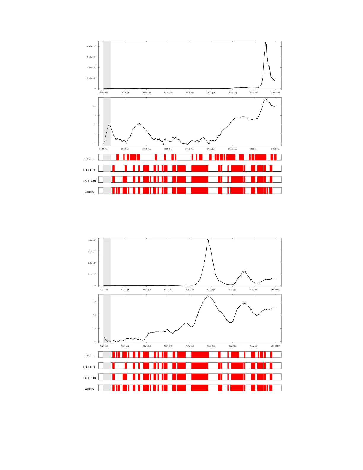
Submitted to the Annals of Applied Statistics ONLINE FDR CONTR OLLING PR OCEDURES FOR ST A TISTICAL SIS MODEL AND ITS APPLICA TION T O CO VID19 D A T A B Y S E O H W A H W A N G 1 , J U N Y O N G P A R K 1 , a 1 Department of Statistics, Seoul National University, a junyongpark@snu.ac.kr W e propose an online false discovery rate (FDR) controlling method based on conditional local FDR (LIS), designed for infectious disease datasets that are discrete and exhibit complex dependencies. Unlike exist- ing online FDR methods, which often assume independence or suffer from low statistical po wer in dependent settings, our approach effecti vely controls FDR while maintaining high detection power in realistic epidemic scenar- ios. F or dise ase modeling, we establish a Dynamic Bayesian Network (DBN) structure within the Susceptible-Infected-Susceptible (SIS) model, a widely used epidemiological frame work for infectious diseases. Our method requires no additional tuning parameters apart from the width of the sliding window , making it practical for real-time disease monitoring. From a statistical per- spectiv e, we prov e that our method ensures valid FDR control under sta- tionary and ergodic dependencies, extending online hypothesis testing to a broader range of dependent and discrete datasets. Additionally , our method achiev es higher statistical power than existing approaches by le veraging LIS, which has been shown to be more powerful than traditional p -value-based methods. W e validate our method through extensi ve simulations and real- world applications, including the analysis of infectious disease incidence data. Our results demonstrate that the proposed approach outperforms exist- ing methods by achie ving higher detection power while maintaining rigorous FDR control. 1. Introduction. Monitoring infectious disease spread in real time is a central task in public health surveillance. During the CO VID-19 pandemic, many countries released daily confirmed case counts, requiring policymakers to determine when to escalate or relax inter - ventions such as social distancing. Howe ver , short-term increases in reported cases do not always indicate a true surge in transmission: transient fluctuations caused by reporting delays or day-of-week ef fects can obscure the underlying trend. For instance, daily increases in incidence may occur even amid an ov erall decline, while true upward trends may be hidden by noise or administrativ e lags. Relying on ad-hoc thresh- olds or short-term fluctuations to guide policy decisions can lead to premature or delayed responses, emphasizing the need for statistically rigorous tools that distinguish sustained in- creases from random variation. This paper introduces a robust statistical framew ork that inte- grates online FDR controlling procedures with a probabilistic formulation of the Susceptible- Infected-Susceptible (SIS) epidemiological model, structured within a Dynamic Bayesian Network (DBN). This synthesis allows for the sequential analysis of incoming data to test, in real-time, whether the number of observed cases is increasing, all while rigorously control- ling for the proportion of false discov eries among all rejected hypotheses. The effecti veness and statistical properties of our proposed methods, in terms of both FDR control and po wer to detect true increases, are first v alidated through extensi ve simulation studies. T o demonstrate the practical utility and broad applicability of our framework, we con- duct a comprehensiv e real-world data analysis using datasets from sources like Our W orld K e ywor ds and phrases: Online FDR, Suscptible-Infected-Susceptible model, Dynamic Bayesian Netow ork, CO VID-19. 1 2 in Data. Our analysis includes a deliberately div erse set of infectious diseases: CO VID-19, influenza, chickenpox, Mycoplasma pneumoniae, Dengue Fever , Hand, Foot, and Mouth Dis- ease (HFMD), and Hepatitis E. This selection allows for a rob ust e v aluation of our method’ s performance across varied epidemiological contexts, including different transmission mech- anisms and data reporting structures. The application of our model to this di verse set of pathogens serves two key purposes. First, it tests the model’ s performance across v arious transmission dynamics. For diseases characterized primarily by direct person-to-person contact where reinfection is possible (CO VID-19, influenza, HFMD, chickenpox), the SIS model is a fundamentally well-suited frame work. For diseases with more complex transmission pathw ays, such as the v ector-borne Dengue Fe ver or the waterborne Hepatitis E, our applicat ion of the SIS model tests its utility as a robust, first-order surveillance tool. In these cases, the model’ s transmission parameter acts as an effecti v e aggregate measure that captures the net result of the more complex under- lying epidemiological processes, ev en without explicitly modeling vectors or en vironmental reservoirs. Second, this disease selection inherently includes data with different temporal granularities, from daily reporting (e.g., CO VID-19) to weekly reporting (e.g., influenza, Dengue Fe ver). This v ariation allo ws us to demonstrate the flexibility of our online proce- dure, which is designed to sequentially process observations as they arriv e, regardless of the specific time interval between them. This highlights its practical value for real-world public health data streams, which are often inconsistent in their reporting frequency . The remainder of this paper is organized as follo ws. Section 2 re vie ws the limitations of classical SIS models and existing online FDR-controlling procedures. Section 3 introduces a stochastic reformulation of the SIS model and describes how we modify its structure to enable statistical inference and hypothesis testing. Section 4 presents our proposed online testing procedure, which le verages temporal dependence through a latent-state frame work to enhance detection power , and establishes its theoretical properties. Section 5 reports simu- lation results under various scenarios, including cases with seasonal effects and model mis- specification. Section 6 provides a real data analysis on infectious diseases with div erse in- fection durations and transmission routes, demonstrating the practical utility of our method. Concluding remarks and directions for future work are pro vided in Section 7 . 2. Literature Re view . 2.1. Limitations of Classical SIS for Real-T ime Monitoring. The Susceptible–Infectious– Susceptible (SIS) model is a classical framework used to describe the spread of infectious diseases ( Kermack and McKendrick , 1927a ). It partitions a fixed population of size N into susceptible indi viduals S t and infected individuals I t at each time t . Infections occur through contact with the infected, and recov ered indi viduals return to the susceptible pool. Under a discrete-time formulation, the dynamics e volv e via: S t +1 = S t − S t · ˜ γ I t N + 1 d I t , (2.1) I t +1 = S t · ˜ γ I t N +  1 − 1 d  I t , (2.2) where ˜ γ is the per-contact transmission rate, and 1 /d is the recovery rate corresponding to an av erage infectious duration of d days. While useful for long-term forecasting, this deterministic model assumes a constant trans- mission rate ov er time and lacks flexibility for real-time inference. In practical surveillance settings, policymak ers often ask a simpler question: Is the epidemic currently accelerating? That is, does the ef fectiv e reproduction number γ t := d ˜ γ t exceed 1 at time t ? ONLINE FDR CONTR OLLING PR OCEDURES FOR ST A TISTICAL SIS MODEL 3 A natural formulation is the sequence of hypotheses: H 0 t : γ t ≤ 1 vs. H 1 t : γ t > 1 . Ho wev er , testing this hypothesis directly is problematic. Estimating γ t using the plug-in ratio ˆ γ t = J t /I t (where J t is the number of new infections and I t an estimate of current infectious indi viduals per day) reduces the hypothesis test to a trivial threshold comparison between J t and I t : if J t ≫ I t , H 0 t is rejected, which ignores temporal structure or uncertainty . 2.2. Dynamic Bayesian Networks (DBNs) . A Dynamic Bayesian Network (DBN) is a probabilistic graphical model that extends the formalism of Bayesian Networks (BNs) to rep- resent and reason about temporal processes. While a standard BN models the probabilistic dependencies among a set of variables at a single point in time, a DBN provides a com- pact representation of the joint probability distribution ov er sequences of v ariables ev olving through time ( Murphy , 2002 ). Formally , a DBN models the distribution over a collection of time-indexed random vari- ables Z t = { Z 1 t , . . . , Z n t } . The model is defined by a pair of a prior network and a transition network. 1. A prior network , specifies the joint probability distrib ution ov er the state variables for the initial time steps required by the model’ s dependency structure. 2. A transition network , defines the conditional probability distribution of the state v ari- ables at time t gi ven the state over the d preceding time steps, denoted as P ( Z t | Z t − d , . . . , Z t − 1 ) . In this work, we generalize the con ventional first-order dependency and employ a d th- order Marko v assumption, where the state of the system at time t is conditionally independent of the distant past giv en the states of the previous d time steps ( Murphy , 2002 ). That is, for t ≥ d : (2.3) P ( Z t | Z 0 , . . . , Z t − 1 ) = P ( Z t | Z t − d , . . . , Z t − 1 ) The transition network’ s parameters and structure are assumed to be time-inv ariant (station- ary), meaning the rules gov erning the system’ s e volution do not change ov er time. By un- rolling this network over T time steps, the DBN defines a full joint probability distrib ution ov er the trajectory Z 0: T ≡ { Z 0 , Z 1 , . . . , Z T } ( K oller and Friedman , 2009 ). The selection of the DBN frame work for our method is motiv ated by sev eral key ad- v antages that directly facilitate our proposed methodology . First, the graphical structure of a DBN provides an intuiti ve and explicit representation of the model’ s underlying as- sumptions. This visual clarity enhances interpretability , making the causal relationships be- tween variables—such as the infectious pool ( I t ), the latent trend ( θ t ), and new infections ( J t )—transparent. Second, DBNs offer a natural frame work for integrating latent variables. This is crucial for our method, where the central hypothesis rev olves around inferring an unobserv able epidemic trend, θ t . The DBN formalizes this trend as a hidden state within a generati ve process, allowing us to reason about the underlying dynamics driving the observ- able case counts. Finally , and most critically , the DBN structure provides a principled and computationally tractable foundation for probabilistic inference. The explicitly defined dependencies allow for the application of efficient, exact algorithms for tasks such as filtering and smooth- ing. For our method, this is a paramount benefit, as the framew ork enables the use of the forward-backward algorithm to compute the posterior probability of the latent state, P ( θ t | J 1 , . . . , J T ) . This probability is essential as it forms the basis of the Local Index of Significance (LIS), the core test statistic for our online FDR controlling procedure ( Efron , 4 2005 ; Sun and Cai , 2007 ). Therefore, the DBN acts as the crucial computational engine that makes our statistical tests feasible. Due to their capacity to model temporal dependencies and incorporate latent (unobserved) v ariables, DBNs are exceptionally well-suited for modeling complex dynamic systems, in- cluding those found in epidemiology . In this work, the DBN framew ork is le veraged to repre- sent the stochastic Susceptible-Infected-Susceptible (SIS) dynamics and to perform inference on a latent state v ariable representing the underlying epidemic trend. 2.3. Online T esting. A widely studied frame work for online false discovery rate (FDR) control is the alpha-in vesting algorithm introduced by Foster and Stine ( 2008 ). This approach allocates a pre-specified "alpha-wealth" budget across sequential hypothesis tests. When a test results in a rejection, the procedure earns back some alpha wealth, enabling it to continue testing. This adaptive strategy allows for real-time updates to the significance le vel while maintaining FDR control. Subsequent works have extended the alpha-in vesting framew ork. In particular , methods such as LORD++ ( Ramdas et al. , 2017a ), SAFFR ON ( Ramdas et al. , 2018 ), and ADDIS ( T ian and Ramdas , 2019 ) reward successful rejections by dynamically increasing the alpha budget. These approaches offer greater flexibility and statistical power compared to static procedures. Despite their innovation, alpha-inv esting algorithms suffer from well-documented issues such as alpha-death (where no ne w rejections occur due to a depleted alpha budget) and pig- gybacking (where large alpha rewards lead to overly aggressi ve rejections) ( Ramdas et al. , 2017b ). T o mitigate these challenges, Gang, Sun and W ang ( 2023 ) proposed the Structure- Adapti ve Sequential T esting (SAST) framew ork, which b uilds on the conditional local inde x of significance (LIS) and adapts testing thresholds based on local structure in the data. SAST achie ves FDR control under independence and of fers near-optimal power in various struc- tured testing scenarios. Nonetheless, SAST assumes independence among test statistics, an assumption often vio- lated in real-world applications such as infectious disease surveillance, where strong temporal dependence is intrinsic to the data. In such settings, modeling this dependence is critical for reliable detection. 3. Modeling Framework Motiv ated by Classical Infectious Disease Model. 3.1. Stochastic Modeling of Case Counts. W e formulate a stochastic version of the SIS model. Define: • J t : the number of ne w infections at time t ; • I t : the rolling av erage of recent infections, I t = 1 min( d, t ) t X i =max( t − d +1 , 1) J i , as a proxy for the infectious pool; • S t = N − I t : the number of susceptibles, under the assumption I t ≪ N . Gi ven these quantities, we model J t as: J t | ( I t , γ t ) ∼ Binomial  S t , γ t I t N  , and under the standard Poisson approximation (v alid when S t ≈ N ), we write: J t | ( I t , γ t ) ≈ Poisson( γ t I t ) . ONLINE FDR CONTR OLLING PR OCEDURES FOR ST A TISTICAL SIS MODEL 5 This formulation captures daily randomness in case counts while linking them mechanisti- cally to latent transmission dynamics. The infectious pool is updated via a rene wal equation: I t +1 = I t + J t − J t − d +1 , which reflects that indi viduals remain infectious for d days before recov ering. 3.2. Latent T r end Modeling via Hidden States. T o o vercome the instability of estimating γ t for e very t , we introduce a discrete latent state process θ t ∈ { 1 , 2 , 3 } that gov erns the transmission regime. Specifically: • θ t = 1 : decreasing ( γ t < 1 ), • θ t = 2 : stationary ( γ t = 1 ), • θ t = 3 : increasing ( γ t > 1 ). Conditionally on θ t = j , the transmission rate is modeled as: γ t | ( θ t = j ) ≡ γ j The hidden state sequence { θ t } ev olves according to a first-order Markov chain with transi- tion matrix A = [ a ij ] 1 ≤ i,j ≤ 3 and initial distribution π = { π 1 , π 2 , π 3 } as described in Figure 1 . This latent-state framework defines a dynamic Bayesian network (DBN) ov er { θ t , γ t , J t } 𝜃 ! 𝜃 " #! 𝜃 " 𝜃 " $! 𝐽 " 𝐽 " #! 𝐽 " $! 𝐼 " 𝐼 " #! 𝐼 " $! 𝐽 ! 𝐼 ! 𝑎 % !" # ,% ! 𝑎 % ! ,% !$# 𝑡 = 1 𝑡 = 𝑑 − 1 𝑡 = 𝑑 𝑡 = 𝑑 + 1 F I G 1 . Dynamic Bayesian network (DBN) for the pr oposed model with latent state sequence { θ t } t ≥ 1 . The initial distribution is P ( θ 1 = i ) = π i for i ∈ { 1 , 2 , 3 } , and the transition law is P ( θ t +1 = i | θ t = j ) = a ij for i, j ∈ { 1 , 2 , 3 } . and allows for posterior inference via EM and forward-backw ard algorithms. It captures time- v arying epidemic trends while av oiding day-to-day ov erfitting. 3.3. Statistical Hypothesis T esting Based on P osterior Infer ence. Instead of testing di- rectly on γ t , we test the latent trend state: H 0 t : θ t ∈ { 1 , 2 } vs. H 1 t : θ t = 3 . This reframing allows us to use Bayesian posterior probabilities to dri ve decisions. Let D t denote observed data in a window prior to time t , and define the local index of significance (LIS): L t := P ( θ t ∈ { 1 , 2 } | D t ) , 6 as a probabilistic measure of e vidence against the alternative. A small value of L t suggests strong e vidence that θ t = 3 , indicating a supercritical trend. This probabilistic formulation provides a natural test statistic for real-time monitoring and enables control of the false discov ery rate (FDR) over time using recent advances in online multiple testing, as we detail in Section 4 . 4. Proposed Method. Building on the latent-state SIS model introduced in Section 2.1 , we now describe how to implement this framework for real-time epidemic monitoring. Our goal is to sequentially test for increases in transmission while controlling the false discovery rate (FDR) across time. This section details the statistical model, parameter estimation via the EM algorithm, and an online testing procedure based on Structure-Adapti ve Sequential T esting (SAST + ). 4.1. Pr epr ocessing via STL Decomposition (Optional). T o remove weekly seasonality in the raw incidence data J t , we apply Seasonal-T rend Decomposition using LOESS (STL) ( Cle veland et al. , 1990 ). W e decompose the log-intensity log γ t into: log γ t = T t + S t , where T t captures the long-term trend and S t the seasonal component. T o focus estimation on the trend, we adjust I t by rescaling: e I t := I t · exp( S t ) , and treat γ t e I t as the effecti ve Poisson mean. This preprocessing isolates trend-driven devia- tions. 4.2. P arameter Estimation via the EM Algorithm. W e estimate the model parameters (4.1) ν = { ( γ j ) 1 ≤ j ≤ 3 , ( A ij ) 1 ≤ i,j ≤ 3 , ( π j ) 1 ≤ j ≤ 3 } via the Expectation-Maximization (EM) algorithm. Gi ven the observed data { J t , I t } T t =1 and the latent epidemic state { θ t } T t =0 , the complete-data likelihood under parameter ν is gi ven by: (4.2) P ν ( J 1: T , θ 1: T ) = π θ 1 · T Y t =2 A θ t − 1 ,θ t · T Y t =1 P oisson( J t ; γ θ t I t ) . The EM algorithm alternates between the follo wing steps until con ver gence: E-step. Compute the expected complete-data log-likelihood under the current parameter ν ( m ) : Q ( ν ( m +1) | ν ( m ) ) = E ν ( m ) [log P ν ( m +1) ( J 1: T , θ 1: T ) | J 1: T ] = 3 X j =1 P ( θ 1 = j | J 1: T ) · log π ( m +1) j + 3 X i,j =1 T X t =1 P ( θ t − 1 = i, θ t = j | J 1: T ) · log A ( m +1) ij + 3 X j =1 T X t =1 P ( θ t = j | J 1: T ) · n − γ ( m +1) j I t + J t log( γ ( m +1) j I t ) − log ( J t !) o . (4.3) ONLINE FDR CONTR OLLING PR OCEDURES FOR ST A TISTICAL SIS MODEL 7 T o compute the marginal and joint posteriors of θ t , we apply the forward-backward algo- rithm. Let α i ( t ) and β i ( t ) be the forward and backw ard probabilities defined as: α i ( t ) = P ( J 1: t , θ t = i ) =   3 X j =1 α j ( t − 1) A j i   · Poisson( J t ; γ i I t ) , (4.4) β i ( t ) = P ( J t +1: T | θ t = i ) = 3 X j =1 A ij · Poisson( J t +1 ; γ j I t +1 ) · β j ( t + 1) , (4.5) with initialization α i (1) = π i · Poisson( J 1 ; γ i I 1 ) , β i ( T ) = 1 . The marginal posterior is then computed by (4.6) P ( θ t = i | J 1: T ) = α i ( t ) · β i ( t ) P 3 j =1 α j ( t ) · β j ( t ) . The joint posterior is gi ven by: (4.7) P ( θ t = i, θ t +1 = j | J 1: T ) = α i ( t ) · A ij · Poisson( J t +1 ; γ j I t +1 ) · β j ( t + 1) P k,l α k ( t ) · A kl · Poisson( J t +1 ; γ l I t +1 ) · β l ( t + 1) . M-step. Using the posterior estimates from the E-step, we update the parameters in closed form: π ( m +1) j = P ν ( m ) ( θ 1 = j | J 1: T ) , (4.8) A ( m +1) ij = P T t =1 P ν ( m ) ( θ t − 1 = i, θ t = j | J 1: T ) P T t =1 P ν ( m ) ( θ t − 1 = i | J 1: T ) , (4.9) γ ( m +1) j = P T t =1 P ν ( m ) ( θ t = j | J 1: T ) · J t P T t =1 P ν ( m ) ( θ t = j | J 1: T ) · I t . (4.10) These updates are derived by maximizing each component of the Q-function ( 4.3 ), subject to the normalization constraints on π and A . Full deri vations are pro vided in the supplemen- tary material. The EM procedure iterates between computing ( 4.6 )–( 4.7 ) and applying the closed-form updates ( 4.8 )–( 4.10 ) until conv ergence. The complete algorithm is summarized in Algorithm 1 , and additional details of the EM procedure are gi ven in Appendix ?? . 8 Algorithm 1: EM Algorithm for statSIS model Input : Observed data { J t , I t } T t =1 , initial parameters ν (0) = ( π (0) , A (0) , γ (0) ) , tolerance ϵ Output: Estimated parameters ν = ( π , A, γ ) 1 Initialize: m ← 0 2 repeat 3 E-step: Compute f orward α i ( t ) and backward β i ( t ) : 4 α i (1) ← π ( m ) i · Poi( J 1 ; γ ( m ) i I 1 ) 5 f or t = 2 , . . . , T do 6 α i ( t ) ← P j α j ( t − 1) A ( m ) j i · Poisson( J t ; γ ( m ) i I t ) 7 β i ( T ) ← Poisson ( J T ; γ ( m ) i I T ) 8 f or t = T − 1 , . . . , 1 do 9 β i ( t ) ← P j A ( m ) ij · Poisson( J t +1 ; γ ( m ) j I t +1 ) · β j ( t +1) 10 P ν ( m ) ( θ t = i | J 1: T ) ← α i ( t ) β i ( t ) P k α k ( t ) β k ( t ) 11 P ν ( m ) ( θ t = i, θ t +1 = j | J 1: T ) ← α i ( t ) A ( m ) ij Poisson( J t +1 ; γ ( m ) j I t +1 ) β j ( t +1) P k,ℓ α k ( t ) A ( m ) kℓ Poisson( J t +1 γ ( m ) ℓ I t +1 ) β ℓ ( t +1) 12 M-step: Update parameters using closed-f orm expressions: 13 π ( m +1) j ← P ν ( m ) ( θ 0 = j | J 1: T ) 14 A ( m +1) ij ← P T − 1 t =1 P ν ( m ) ( θ t = i,θ t +1 = j | J 1: T ) P T − 1 t =1 P ν ( m ) ( θ t = i | J 1: T ) 15 γ ( m +1) j ← P T t =1 P ν ( m ) ( θ t = j | J 1: T ) · J t P T t =1 P ν ( m ) ( θ t = j | J 1: T ) · I t 16 m ← m + 1 17 until ∥ ν ( m +1) − ν ( m ) ∥ < ϵ ; 4.3. Online T esting Pr ocedur e Contr olling FDR. W e propose a modified version of Structure-Adapti ve Sequential T esting (SAST ; Gang, Sun and W ang , 2023 ), denoted as SAST + , tailored to temporally dependent and discrete data from hidden-state epidemic mod- els. Unlike the original SAST , which assumes i.i.d. and continuous observations, SAST + incorporates parametric estimation and latent Marko vian structure. At each time T , we test the null hypothesis: H 0 T : θ T ∈ { 1( decr easing ) , 2( stationar y ) } vs. H 1 T : θ T ∈ { 3( incr easing ) } , using the recent data windo w J ( T − h +1): T of size h . W e define the local null probability: L T ( ν ) = P ν ( θ t ∈ { 1 , 2 } | J ( T − h +1): T ) , which quantifies the posterior probability that time t belongs to a non-increasing regime. Since the parameter ν is unkno wn, we estimate it using the EM algorithm (Algorithm 1 ) to obtain: L T ( ˆ ν T ) = P ˆ ν T ( θ T ∈ { 1 , 2 } | J ( T − h +1): T ) . These values are computed for all t ∈ { T − h + 1 , . . . , T } , sorted in ascending order L (1) ≤ · · · ≤ L ( h ) , and used to define the adapti ve threshold: ˆ λ T = L ( k ) , where k = max ( t ≤ h : 1 t t X i =1 L ( i ) ≤ α ) . W e reject H 0 T if: ONLINE FDR CONTR OLLING PR OCEDURES FOR ST A TISTICAL SIS MODEL 9 1. L T ( ˆ ν T ) ≤ ˆ λ T , and 2. The av erage of all rejected L t ’ s including L T does not exceed α : 1 |R T − 1 | + 1   X t ∈R T − 1 L t ( ˆ ν t ) + L T ( ˆ ν T )   ≤ α. This procedure av oids backward correction and uses only current estimates, ensuring real- time applicability . The full process is gi ven in Algorithm 2 . Algorithm 2: SAST+ Input : Counts J 1: T , window size h , Significance le vel α Output: Rejected set R T 1 Initialization: 2 Estimate ˆ ν h using Algorithm 1 on J 1: h 3 Compute L t ( ˆ ν h ) = P ˆ ν h ( θ t ∈ { 1 , 2 } | J 1: h ) for t = 1 , . . . , h 4 Sort { L t ( ˆ ν h ) } ascending: L (1) ( ˆ ν h ) ≤ · · · ≤ L ( h ) ( ˆ ν h ) 5 Set ˆ λ h ← max n L ( k ) ( ˆ ν h ) : 1 k P k i =1 L ( k ) ( ˆ ν h ) ≤ α o 6 Reject H 0( t ) if L t ( ν T ) ≤ ˆ λ h 7 Set R h = { t ≤ h : H 0 t rejected } 8 for T = h + 1 , . . . , T do 9 Estimate ˆ ν T from J T − h +1: T using Algorithm 1 10 Compute L t ( ˆ ν T ) = P ˆ ν T ( θ t ∈ { 1 , 2 } | J T − h +1: T ) for t = T − h + 1 , . . . , T 11 Sort ( L t ( ˆ ν T )) T − h +1 ≤ t ≤ T ascending 12 Set ˆ ν T ← max n L ( k ) ( ˆ ν T ) : 1 k P k i =1 L ( i ) ( ˆ ν T ) ≤ α o 13 Reject H 0 T if both conditions hold: 14 (C1) L T ( ˆ ν T ) ≤ ˆ λ T , 15 (C2) 1 |R T − 1 | +1  P t ∈R T − 1 L t ( ˆ ν t ) + L T ( ˆ ν T )  ≤ α 16 Update: R T ← R T − 1 ∪ { T } if rejected, else R T ← R T − 1 4.4. Theor etical Results. W e no w present theoretical guarantees that support the use of this method under dependence. Under mild conditions, we show that the adapti ve barrier ˆ λ T is asymptotically the best gate-keeping threshold, and that SAST + asymptotically controls FDR at the desired le vel. T o formalize this idea, we define the function Q ( λ ) , which quantifies the marginal false discov ery proportion (FDP) when all hypotheses with LIS less than or equal to λ are rejected. Specifically , Q ( λ ) = p 0 G 0 ( λ ) G ( λ ) , where p 0 = P ( θ t ∈ { 1 , 2 } ) , G 0 ( λ ) = P ( L t ( ν ) ≤ λ | θ t ∈ { 1 , 2 } ) , G ( λ ) = P ( L t ( ν ) ≤ λ ) . Here, the numerator p 0 G 0 ( λ ) corresponds to the expected proportion of false discov eries (i.e., true nulls rejected) at threshold λ , and the denominator G ( λ ) gi v es the o verall rejection probability . Hence, Q ( λ ) represents the expected FDP among all rejections made at that threshold. 10 The optimal barrier for FDR control is characterized by λ ∗ = sup { λ ∈ [0 , 1] : Q ( λ ) ≤ α } . In of fline settings—where all LIS values are kno wn in adv ance—we can sort them and di- rectly identify the largest rejection set that satisfies the FDR constraint. Ho wev er , in online settings, only past LISs are observ able at each step. This limited access leads to partial or - dering and can cause inconsistencies: a hypothesis with a lower LIS may remain unrejected while one with a higher LIS is rejected. T o address this, SAST introduces a barrier —a gate-keeping threshold that restricts rejec- tions to hypotheses with LIS values below a data-driv en lev el ( Gang, Sun and W ang , 2023 ). This threshold is updated adaptively based on observed LISs. Notably , the barrier itself does not need to exactly control the FDR. Instead, it is chosen to be slightly larger than the cutoff which controls FDR, providing higher po wer . In the continuous setting—considered in Gang, Sun and W ang ( 2023 )—the value λ ∗ cor- responds to the lar gest threshold such that rejecting all hypotheses with L t ( ν ) ≤ λ ∗ keeps the FDR within lev el α . W e extend the role of barrier to the discrete setting, which commonly arises in practical applications. In such cases, λ ∗ may not exactly control FDR, and instead can be interpreted as the smallest one beyond which Q ( λ ) > α . T H E O R E M 4.1 (Adaptiv e Barrier). Assuming the following assumptions hold: A1 The sequence of random variables θ t forms a Marko v chain that is irr educible, aperiodic, and stationary . This Markov chain is characterized by ν 0 , which lies within the interior of the parameter space . Mor eover , { J t } is also irr educible, aperiodic and stationary . A2 F or any parameter set ν , let A r epr esent the transition matrix and π denote the initial pr obability within set ν . Then, ther e exist δ > 0 and ϵ > 0 such that for all ∥ ν − ν 0 ∥ < δ and i, j = 1 , 2 , 3 , we have A ij , π i > ϵ . A3 The maximum likelihood estimator ˆ ν is a consistent estimator of the true parameter set ν 0 . A4 Q ( λ ) is a decr easing function of λ . Applying Algorithm 2 , the adaptive barrier obtained with significance level α satisfies at least one of the followings: • If Q ( λ ∗ ) > α , then ˆ λ T p → λ ∗ as T → ∞ wher e p → r epr esents the conver gence in pr oba- bility . • If Q ( λ ∗ ) = α , then for any ϵ > 0 , P ( ˆ λ T ∈ [ λ − ϵ, λ ∗ + ϵ ]) → 1 wher e λ = inf { λ : Q ( λ ) = lim ϵ ↘ 0 Q ( λ ∗ − ϵ ) } . P RO O F . The complete proof is presented in the supplementary material Section ?? . T H E O R E M 4.2 (FDR control) . Assume that maximum likelihood estimator ˆ ν is a consis- tent estimate of true parameter set ν 0 . Then Algorithm 2 allows for the contr ol of the F alse Discovery Rate (FDR) of the entir e sequence ( L T ( ˆ ν T )) T = h +1 ,h +2 ,... at a level of α + o (1) . P RO O F . The complete proof is provided in the supplementary material ?? . 5. Simulation Study . T o e valuate our proposed method, simulations were performed under various setups. In addition, the effect of model misspecification was inv estigated to assess the robustness of our proposed models. ONLINE FDR CONTR OLLING PR OCEDURES FOR ST A TISTICAL SIS MODEL 11 F I G 2 . Generated data with a fixed seed ( seed = 1 ) and par ameter values ( γ 1 , γ 2 , γ 3 ) = (0 . 8 , 1 , 1 . 2) . The left plot shows the tr end without seasonal effects, while the right plot includes seasonal effects, highlighting periodic fluctuations. The shaded ar eas indicate periods of incr easing values, r epr esenting days that should be r ejected. The infectious period, denoted as d , is established at 7 days. This value is typically well- established and disease-specific, so we assume that this period d is known. The transition matrix has been structured to fav or its diagonal v alues as shown in ( 5.1 ). Unlike the infectious period d , we need to estimate the transition matrix denoted by A which is set to be (5.1) A =   0 . 60 0 . 30 0 . 10 0 . 05 0 . 80 0 . 15 0 . 05 0 . 15 0 . 80   to represent the slight increasing trend of J t ov er time. Subsequently , we’ll e valuate our pro- posed model with various configurations of γ 1 and γ 3 with γ 2 = 1 satisfying γ 1 < 1 < γ 3 . An- other consideration is to ensure the effecti ve remov al of any weekly cyclical patterns within our data. Although our approach presumes a successful adjustment of this periodicity , it’ s important to v alidate the ef fectiv eness of such an adjustment. T o denote the week periodicity , we referred to ( 4.1 ) which uses exp( S t ) . Since we ha ve S t = S t + d for d = 7 , we need only ( S 1 , S 2 , . . . , S 7 ) which are corresponding to (Mon, T ues, . . . , Sun). W e use (5.2) ( S 1 , S 2 , . . . , S 7 ) =  1 10 , 1 20 , 0 , 0 , 0 , − 1 10 , − 1 20  for modeling the weekly effect. The reason for providing these values is that the number of tests is lo west on weekends, resulting in the lo west reported number of disease cases. On the other hand, there is often a rebound in reported cases o ver the next two days (Monday and T uesday). From W ednesday to Friday , the number of cases tends to remain relativ ely stable. These fluctuations are assumed to be unkno wn and their effects are remo ved after estimation. The Figure 2 illustrates the generated data with a fixed random seed ( seed = 1 ) and parameter values ( γ 1 , γ 2 , γ 3 ) = (0 . 8 , 1 , 1 . 2) . The plot on the left sho ws the trend of the data without seasonal effects, pro viding a clear baseline representation of the underlying trend. In contrast, the plot on the right incorporates seasonal ef fects, highlighting periodic fluctuations superimposed on the trend. Additionally , the shaded areas in both plots indicate periods of increasing that should be rejected. This side-by-side comparison emphasizes the impact of seasonal components on the data and ho w they interact with the overall trend. W e consider the situation that data come in online over a period of 530 days, and the simulation will be repeated 500 times to compare the FDR and the statistical power of tests such as TPR(T rue Positi ve Rate) which is defined in the following section. Our proposed methods are applied with the same windo w size h = 30 . W e test the hypotheses H 0 T for 31 ≤ T ≤ 530 where each hypothesis H 0 T is tested based on the data observed J 1: T = { J 1 , . . . , J T } . 12 5.1. Simulation Results of Online T esting . W ithout seasonal ef fect, dif ferent pa- rameter set-ups are considered: ( γ 1 , γ 2 , γ 3 ) = (0 . 8 , 1 , 1 . 2) , (0 . 85 , 1 , 1 . 15) , (0 . 9 , 1 , 1 . 1) and (0 . 95 , 1 , 1 . 05) . As the dif ference γ 3 − γ 1 is smaller , it is more dif ficult to distinguish the null and alternati ve hypotheses. T able 1 - 2 sho ws the estimated FDR and po wer , the T rue Positi ve Rate (TPR) which has the follo wing definition : T P R = E P t ∈R T ∩{ 31 , 32 ,..., 530 } I ( θ t = 3) ( P 530 t =31 I ( θ t = 3)) ∨ 1 ! (5.3) and an estimator of T P R denoted by [ T P R is obtained from Monte Carlo simulation. These results hav e been compared with • an ‘oracle’ setting where all parameters in ν defined in ( 4.1 ) are known and tested in offline setting with all 530 data is observed at once, • Existing online FDR-controlling procedures, including LORD++ ( Ramdas et al. , 2017a ), SAFFR ON ( Ramdas et al. , 2018 ), and ADDIS ( T ian and Ramdas , 2019 ), which operate on p -values. For these methods, we compute the p -v alue at each time t as p t = 1 − F I t ( J t ) , where F I t denotes the cumulativ e distribution function (CDF) of the Poisson distribution with mean I t . Note that these p -value-based methods do not guarantee FDR control at le vel α in the presence of temporal dependence, which is inherent in our application setting. Combining with the proposed online procedures, SAST+, the FDR is generally well controlled for most parameter settings in T able 1 , and the estimated powers ( [ T P R ) are slightly lower than those of the oracle procedure. Online testing methods based on p -v alues sho w comparable power with SAST+ in most cases except the case when ( γ 1 , γ 2 , γ 3 ) = (0 . 95 , 1 , 1 . 05) . Due to the presence of seasonal effects, decision-making becomes more challenging, as demonstrated by the oracle procedures in T able 2 . Consequently , the FDR increases across all methods. Among these, LORD++, SAFFR ON, and ADDIS fail to control the FDR, while SAST+ successfully controls the FDR at the target lev el of α = 0 . 05 , e xcept in cases where the true γ i v alues are closely aligned. This suggests that the STL decomposition may con- tribute to increased noise. T A B L E 1 Simulation r esults without seasonal effects. Oracle SAST+ LORD SAFFR ON ADDIS ( γ 1 , γ 2 , γ 3 ) \ F DR [ T P R \ F DR [ T P R \ F DR [ T P R \ F DR [ T P R \ F DR [ T P R (0.8, 1, 1.2) 0.000 1.000 0.000 1.000 0.004 1.000 0.031 1.000 0.042 1.000 (0.85, 1, 1.15) 0.001 1.000 0.000 1.000 0.004 1.000 0.032 1.000 0.042 1.000 (0.9, 1, 1.1) 0.015 1.000 0.001 0.998 0.004 0.993 0.032 0.998 0.042 0.998 (0.95, 1, 1.05) 0.058 0.978 0.045 0.931 0.004 0.650 0.031 0.837 0.041 0.839 T A B L E 2 Simulation r esults with seasonal effects Oracle SAST+ LORD SAFFR ON ADDIS ( γ 1 , γ 2 , γ 3 ) \ F DR [ T P R \ F DR [ T P R \ F DR [ T P R \ F DR [ T P R \ F DR [ T P R (0.8, 1, 1.2) 0.024 0.979 0.038 0.985 0.296 0.999 0.316 0.999 0.333 1.000 (0.85, 1, 1.15) 0.028 0.982 0.036 0.985 0.255 0.997 0.285 0.998 0.309 0.999 (0.9, 1, 1.1) 0.050 0.983 0.042 0.977 0.169 0.977 0.218 0.989 0.251 0.992 (0.95, 1, 1.05) 0.082 0.936 0.090 0.897 0.034 0.640 0.091 0.806 0.109 0.824 ONLINE FDR CONTR OLLING PR OCEDURES FOR ST A TISTICAL SIS MODEL 13 5.2. Simulation Results of Seasonal Effect Adjustment. Although seasonal adjustment is not our primary concern, it can still influence our decisions. T o ev aluate the impact of seasonal adjustment, we ran an additional simulations under misspecified seasonal effect: W e tested the FDR and TPR under misspecified seasonal ef fects. This in v olved generating J t with seasonal ef fects but not adjusting for them prior to estimation, and vice v ersa. T A B L E 3 Simulation r esults with mismatch in the pr esence of seasonal effect (S/E). (+) indicates the presence of S/E and (-) indicates no S/E. Results with corr ectly specified S/E ar e shown in bold. Oracle SAST+ LORD SAFFR ON ADDIS T rue S/E Specified S/E \ F DR [ T P R \ F DR [ T P R \ F DR [ T P R \ F DR [ T P R \ F DR [ T P R - - 0.000 1.000 0.000 1.000 0.090 1.000 0.113 1.000 0.172 1.000 + 0.022 0.995 0.022 0.976 0.026 0.874 0.054 0.917 0.076 0.934 + - 0.209 0.797 0.197 0.724 0.193 0.761 0.201 0.810 0.219 0.814 + 0.019 0.947 0.042 0.974 0.219 0.999 0.246 0.999 0.287 1.000 T able 3 shows the results of the model analysis in scenarios where seasonal ef fects are either ( i ) present and unadjusted, or ( ii ) absent but adjusted. The results show that account- ing for seasonal effects in the absence of actual seasonal effects increase the FDR and de- crease TPR slightly . Con versely , omitting seasonal adjustment can significantly inflate the FDR while reducing the TPR. These results highlight the importance of appropriately adjust- ing for seasonal effects in the model, and demonstrate that our adjustment of seasonal effect produces robust results e ven in the absence of seasonal effects. 6. Real Data Analysis . T o ev aluate the empirical performance and operational bound- aries of our proposed method (SAST+), we apply it to a di verse set of real-world infectious disease surveillance datasets. These datasets were chosen to represent a range of transmis- sion dynamics and data granularities. W e first validate the method’ s effecti v eness on high- resolution daily CO VID-19 data, which closely aligns with our model’ s assumptions. W e then critically examine its rob ustness and limitations for diseases with different epidemiological characteristics. The performance of SAST+ is benchmarked against three established online FDR-controlling procedures: LORD++, SAFFR ON, and ADDIS. 6.1. P erformance V alidation on High-Resolution Data: The Case of CO VID-19. Our pri- mary validation is conducted using daily CO VID-19 incidence data, which of fers the high- est temporal resolution and aligns well with our model’ s assumptions of a human-to-human transmitted pathogen. W e analyze daily data from Australia and South Korea, obtained from the Our W orld in Data (OWID) repository ( Mathieu et al. , 2020 ). Daily data often exhibits strong periodic ef fects, such as reduced reporting ov er weekends. T o address this, we apply an online STL decomposition as described in Section 4.1 , using a 30-day window at each time point to remove the weekday reporting bias before analysis. W e set the infectious period to d = 7 days and the smoothing window size to h = 30 days. Figures 3 and 4 sho w the daily number of infectious individuals for Australia and South K orea, respectively , alongside the rejection times identified by four online FDR-controlling procedures. The top panel displays the raw data, while the second panel sho ws the same data on a log scale , smoothed with a 7-day moving a verage. In Australia (Figure 3 ), two major epidemic wav es are observed: one from May to Oc- tober 2020 and another from June to October 2021. The first wa ve, from May to October 2020, centered in V ictoria, resulted from breaches in hotel quarantine protocols, peaking in early August. During this period, SAST+ generated early and sustained rejections, effec- ti vely capturing the outbreak onset ahead of other methods. A second major wa v e, from June 14 F I G 3 . Online FDR analysis of daily infectious counts ( J t ) in A ustralia. The top two panels show the raw and the log-scaled/smoothed data, r espectively . Gre y ar eas mark tr aining periods. The lower four panels show the r esults for four differ ent online FDR procedur es, with red marker s indicating r ejection times. F I G 4 . Online FDR analysis of daily infectious counts ( J t ) in South K or ea. The top two panels show the raw and the log-scaled/smoothed data, respectively . Gr ey ar eas mark training periods. The lower four panels show the r esults for four differ ent online FDR procedur es, with red marker s indicating r ejection times. ONLINE FDR CONTR OLLING PR OCEDURES FOR ST A TISTICAL SIS MODEL 15 to October 2021, triggered by the Delta v ariant, was also promptly identified by SAST+, with rejections aligned with the early gro wth of the outbreak. Interestingly , between these wa v es, SAST+ made additional rejections in response to fluc- tuations in imported case risk (e.g., from India in April 2021), where other methods remained inacti ve. This highlights SAST+’ s sensitivity to subtle but epidemiologically meaningful trends. In South Korea (Figure 4 ), the first major outbreak occurred in August 2020 due to church clusters and mass gatherings. This was followed by a large Alpha-v ariant-dri ven wav e in December 2020 and a Delta-driv en surge in mid-2021. In all three episodes, SAST+ detected early and temporally coherent blocks of rejections. Notably , the method adapted its rejection pattern in response to intensified public health interventions such as distancing mandates, with rejection rates declining as case counts stabilized. Overall, these results highlight the adaptive effecti veness of SAST+. While SAST+ clearly outperformed competing methods in coherence and sensiti vity during Australia’ s shifting epidemic, its distinct adv antage was less pronounced in South Korea, where all methods yielded satisfactory and comparable results in identifying outbreak phases. 6.2. Robustness to Reporting Mechanism. W e analyze two diseases that hav e dif ferent reporting requirements to that of CO VID-19: Mycoplasma pneumoniae and influenza. Mycoplasma Pneumoniae and Influenza in K orea are designated as Class 4 infectious dis- eases, requiring reporting within one week. This introduces potential delays and lo wer data precision compared to the daily CO VID-19 dataset. For Mycoplasma Pneumoniae, with an infectious period of 2-4 weeks ( New Y ork State Department of Health ), we set d = 3 and h = 15 weeks. For Influenza, with a typical 7-day infectious period ( Centers for Disease Control and Prevention , 2023 ), we conserv ati vely set d = 2 and h = 8 weeks. As shown in Figures 5 and 6 , SAST+ ef fecti vely identifies key outbreak periods. For Mycoplasma, it makes the most rejections (51) and best captures prolonged increasing trends. For Influenza, its detections (34) form more connected blocks during surges than the more fragmented dis- cov eries of other methods. This affirms the method’ s utility for standard public health surveil- lance systems that rely on weekly reporting. Robustness to Model Misspecification: A pplication to an SIR-T ype Disease T o challenge the foundational assumptions of our proposed method, we test its perfor - mance on data for Chickenpox, a disease whose transmission dynamics represent a techni- cal violation of our model’ s frame work. Our method is designed based on the Susceptible- Infectious-Susceptible (SIS) model, which assumes that individuals return to the susceptible state after recov ering from an infection. This framework is well-suited for diseases that do not confer long-term immunity . In contrast, Chickenpox confers lifelong immunity upon recov ery , making it a classic example of a disease best described by the Susceptible-Infectious-Recov ered (SIR) model K ermack and McKendrick ( 1927b ). The SIR model, originally dev eloped by K ermack and McK endrick, compartmentalizes a population into three distinct groups: Susceptible (S), in- di viduals who can contract the disease; Infectious (I), those who currently hav e the disease and can transmit it; and Recovered (R), indi viduals who have reco vered and are now perma- nently immune. The key distinction from the SIS model is the transition from the Infectious to the Reco vered compartment, which removes individuals from the pool of potential future infections. Despite this model mismatch, we posit that an SIS framework can serve as a robust approx- imation for an SIR-type disease under common real-world conditions. The force of infection in our model is approximated by the term ( S t / N ) γ t I t . In a large population ( N ) where the number of acti ve cases ( I t ) is relati vely small, the susceptible pool ( S t ) depletes v ery slo wly . 16 Consequently , the ratio S t / N remains approximately equal to 1 for extended periods, making the simplification acceptable. Furthermore, demographic changes such as births and deaths introduce a natural flux to the population. In many scenarios, the introduction of new susceptible indi viduals into the population via births can hav e a more significant impact on the susceptible pool than its depletion due to infections alone. This demographic turnov er partially mimics the feedback loop of an SIS model by replenishing the susceptible class, thereby mitigating the conceptual violation of the model’ s assumptions. For our analysis of Chickenpox, a Class 2 notifiable disease in K orea with a typical in- fectious period of 5–7 days ( Centers for Disease Control and Pre vention ), we set our model parameters to a 1-week infectious period ( d = 1 ) and a 4-week seasonality horizon ( h = 4 ). The results, illustrated in Figure 7 , show that our SAST+ method successfully captures the re- current surges in cases with connected blocks of rejections (64). This outcome demonstrates the method’ s robustness and practical utility ev en when the underlying disease dynamics do not perfectly align with the theoretical SIS frame work. F I G 5 . J t of Mycoplasma Pnumoniae in South K or ea with 15 weeks of training periods (gr ey), and r ejections by online FDR contr olling pr ocedures (r ed). Robustness to a V ector -borne Disease W e in vestigate a boundary condition where the core assumption of human-to-human trans- mission is violated. W e analyze weekly Dengue Fev er data from Singapore ( Ministry of Health, Singapore , 2024 ), a v ector-borne disease transmitted by mosquitoes. In this case, the SIS model is ill-suited because the force of infection is not primarily dri ven by the number of infectious humans ( I t ) but by external factors like the vector population density , climate, and biting rates, which our model does not include. W e set d = 2 and h = 8 weeks to account for the viremic period ( W orld Health Organization , 2024 ) and reporting lags. While SAST+ identifies the most potential signals (71) in Figure 8 , their alignment with outbreak surges is less consistent than for the directly transmitted diseases. ONLINE FDR CONTR OLLING PR OCEDURES FOR ST A TISTICAL SIS MODEL 17 F I G 6 . J t of Influenza in South K or ea with 8 weeks of training periods (gre y), and rejections by online FDR contr olling pr ocedures (r ed). F I G 7 . J t of Chickenpox in South Kor ea with 4 weeks of training periods (gr ey), and rejections by online FDR contr olling pr ocedures (r ed). This observation highlights a key limitation of applying an SIS-based frame work to this class of infections. The epidemiology of v ector-borne diseases is defined by an indirect trans- mission cycle that requires modeling the vector population itself ( Ross , 1911 ). State-of-the- art models are therefore complex, often incorporating detailed data on vector ecology and en vironmental conditions ( Focks et al. , 1995 ; Andraud et al. , 2012 ). Our method, based on 18 a direct-transmission model, cannot account for these external factors, which weakens its ability to detect surges dri ven by vector dynamics. This finding helps define the scope of our method. It covers many settings e ven the infec- tious diseases with lifelong immunity , but may hav e limited applicability for some vector - borne diseases, where more specialized models are needed for optimal performance. F I G 8 . J t of Dengue in Singapor e with 8 weeks of training periods (gr ey), and r ejections by online FDR contr ol- ling pr ocedur es (r ed). 7. Concluding Remarks. Compared to the traditional SIS method, our approach adopts a probabilistic perspective on epidemiological ev ents rather than the standard deterministic approach. By transforming an SIS model into a Poisson (or binomial) distribution, we can improv e the interpretability between consecutiv e numbers of infectious people. In addition to the statistical SIS model, we suggest online FDR control method, SAST+, which test whether the number of infected individuals tends to increase or not and showed that this procedure can control FDR in online en vironment. This procedure is compared with some existing methods which handle online data de- signed for controlling an y gi ven FDR. The numerical studies sho w that only SAST+ controls FDR and sho ws comparable power with oracle procedure if the model is true. Our empirical e v aluation on real-world data demonstrated the practical utility and opera- tional scope of SAST+. On high-resolution CO VID-19 data, our method sho wed a distinct ad- v antage over traditional change-point detection methods by effecti v ely identifying sustained transmission trends over long periods, a kno wn limitation of methods designed to find only a single change point. Furthermore, our analyses extended beyond this ideal scenario. SAST+ demonstrated strong robustness, performing ef fectively on standard weekly surveillance data for Influenza and Mycoplasma pneumoniae, and e v en when applied to Chickenpox, a disease better described by an SIR model. Crucially , the study also defined the method’ s boundaries. The analysis of Dengue Fe v er , a v ector-borne disease, highlighted the limitations of the SIS- based frame work for indirect transmission routes, where performance was attenuated. ONLINE FDR CONTR OLLING PR OCEDURES FOR ST A TISTICAL SIS MODEL 19 T aken together, these real-world applications not only v alidate the effecti veness of SAST+ for monitoring human-to-human infectious diseases b ut also transparently establish its scope of application. These innov ations make our methods not only accurate and reliable for ana- lyzing trends in diseases like CO VID-19 but also highly adaptable for wider applications in public health surveillance. As future work, we assumed stationary processes which may be somewhat strong condi- tion, so it is of interest to extend the methods to non-stationary processes. Supplementary materials. Supplementary materials include the detailed explanation of EM algorithm and the proofs of all Theorems and Lemmas. Funding. This work was supported by the National Research Foundation of Korea (NRF) grant funded by the K orea gov ernment (MSIT) (RS-2025-00556575). Conflict of Interest. The authors hav e declared no conflict of interest. 8. Data and Code A vailability . The CO VID-19 dataset(O WID) and source code of this paper can be found at the following GitHub repository: https://github .com/IAMSHHW ANG/ statistical_SIS . REFERENCES A N D R AU D , M ., H E N S , N . , M A R A , V . K . and B E U T E L S , P . (2012). Dynamic models of dengue transmission: a systematic revie w of the literature. PLoS ne glected tropical diseases 6 e1859. C L E V E L A N D , R . B . , C L E V E L A N D , W . S . , M C R A E , J . E . , T E R P E N N I N G , I . et al. (1990). STL: A seasonal-trend decomposition. J. Of f. Stat 6 3–73. E F RO N , B . (2005). Local false discov ery rates. F O C K S , D . A ., D A N I E L S , E ., H A I L E , D . G . and K E E S L I N G , J . E . (1995). A dynamic life table model for Aedes aegypti (Diptera: Culicidae): simulation results and v alidation. J ournal of medical entomology 32 293–302. C E N T E R S F O R D I S E A S E C O N T RO L A N D P R E V E N T I O N Chickenpox (V aricella) – T ransmission. Accessed: 2025- 07-20. C E N T E R S F O R D I S E A S E C O N T R O L A N D P R E V E N T I O N (2023). How Flu Spreads. Accessed: 2025-07-20. F O S T E R , D . P . and S T I N E , R . A . (2008). α -in vesting: a procedure for sequential control of expected false dis- cov eries. Journal of the Royal Statistical Society Series B: Statistical Methodolo gy 70 429–444. G A N G , B . , S U N , W . and W A N G , W . (2023). Structure–adaptive sequential testing for online false disco very rate control. Journal of the American Statistical Association 118 732–745. K E R M A C K , W . O . and M C K E N D R I C K , A . G . (1927a). A contribution to the mathematical theory of epidemics. Pr oceedings of the Royal Society of London. Series A, Containing P apers of a Mathematical and Physical Character 115 700–721. K E R M A C K , W . O . and M C K E N D R I C K , A . G . (1927b). A Contribution to the Mathematical Theory of Epidemics. Pr oceedings of the Royal Society of London. Series A, Containing P apers of a Mathematical and Physical Character 115 700–721. https://doi.org/10.1098/rspa.1927.0118 K O L L E R , D . and F R I E D M A N , N . (2009). Pr obabilistic graphical models: principles and techniques . MIT press. M AT H I E U , E . , R I T C H I E , H . , R O D É S - G U I R A O , L . , A P P E L , C . , G I AT T I N O , C . , H A S E L L , J . , M AC D O N A L D , B . , D ATTA N I , S . , B E LT E K I A N , D . , O RT I Z - O S P I N A , E . and R O S E R , M . (2020). Coronavirus P andemic (CO VID- 19). https://ourworldindata.or g/coronavirus . Accessed: 2022-12-12. M I N I S T RY O F H E A LT H , S I N G A P O R E (2024). W eekly Infectious Disease Bulletin Cases. Go vernment of Singa- pore. Retriev ed August 6, 2025, from https://data.gov .sg/dataset/weekly- infectious- disease- bulletin- cases . M U R P H Y , K . P . (2002). Dynamic bayesian networks: repr esentation, inference and learning . Uni versity of Cali- fornia, Berkeley . N E W Y O R K S TA T E D E PA RT M E N T O F H E A LT H Mycoplasma Infection (walking pneumonia, atypical pneumonia) Fact Sheet. W ebsite. Accessed: 2025-07-28. Page last revie wed: No vember 2023. W O R L D H E A LT H O R G A N I Z AT I O N (2024). Dengue and severe dengue. Fact sheet. Retrieved August 6, 2025, from https://www .who.int/news- room/fact- sheets/detail/dengue- and- severe- dengue . R A M D A S , A . , Y A N G , F., W A I N W R I G H T , M . J . and J O R D A N , M . I . (2017a). Online control of the false disco very rate with decaying memory. Advances in neural information pr ocessing systems 30 . 20 R A M D A S , A . , Y A N G , F., W A I N W R I G H T , M . J . and J O R D A N , M . I . (2017b). Online control of the f alse discovery rate with decaying memory. Advances in neural information pr ocessing systems 30 . R A M D A S , A . , Z R N I C , T . , W A I N W R I G H T , M . and J O R D A N , M . (2018). SAFFRON: an adaptive algorithm for online control of the false discovery rate. In International conference on machine learning 4286–4294. PMLR. R O S S , R . (1911). The prevention of malaria. Natur e 88 51–52. S U N , W. and C A I , T. T. (2007). Oracle and adaptive compound decision rules for false discov ery rate control. Journal of the American Statistical Association 102 901–912. T I A N , J . and R A M DA S , A . (2019). ADDIS: an adaptive discarding algorithm for online FDR control with con- servati v e nulls. Advances in neural information pr ocessing systems 32 .