Box Thirding: Anytime Best Arm Identification under Insufficient Sampling

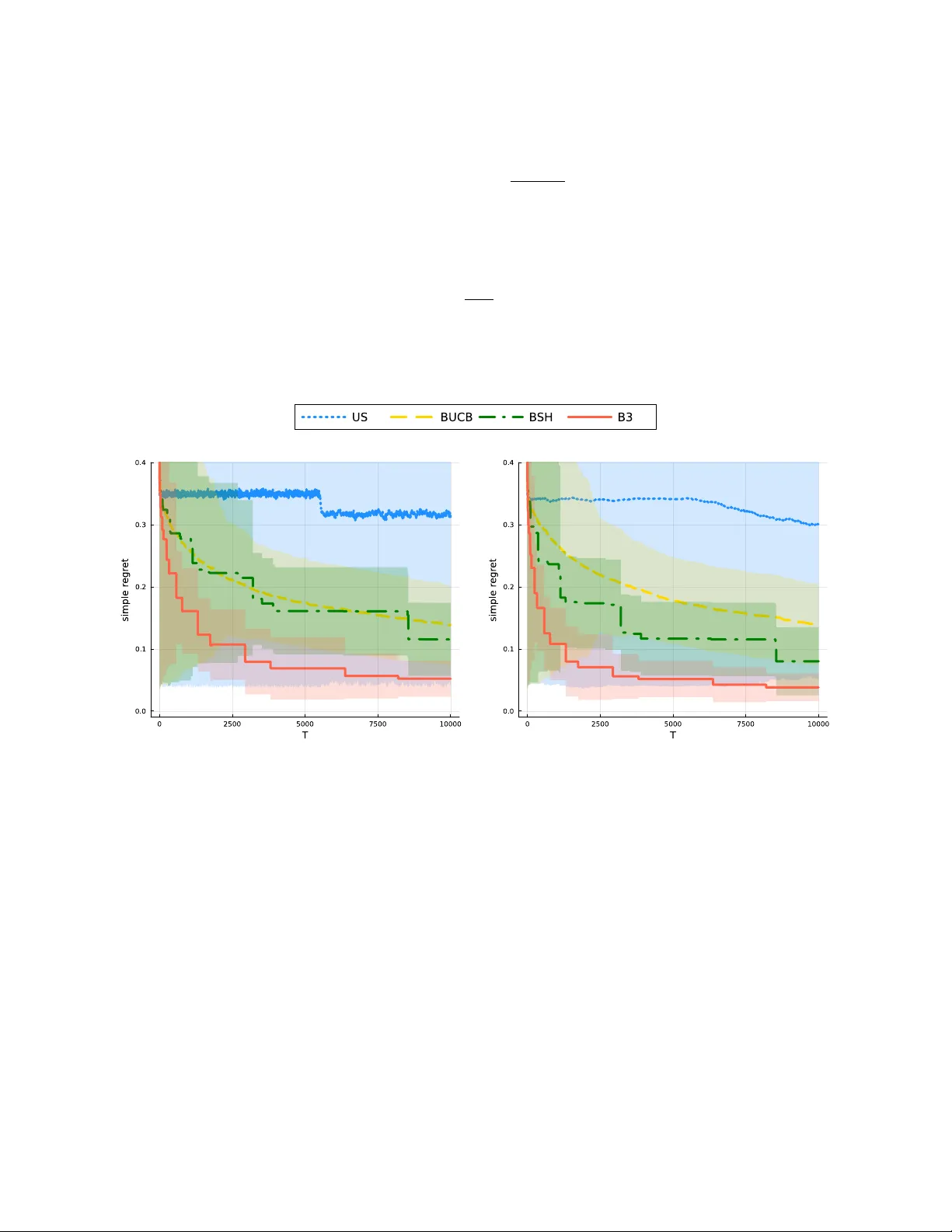
Bo x Thirding: An ytime Best Arm Iden tiﬁcation under Insuﬃcien t Sampling Preprin t. Under review. Seoh wa Hw ang Jun yong P ark Departmen t of Statistics, Seoul National Universit y , Seoul, Republic of Korea junyongpark@snu.ac.kr Keyw ords: Multi-arm Bandit, Best Arm Identiﬁcation, Anytime, Insuﬃcient budget constrain t Abstract W e introduce Box Thirding (B3), a ﬂexible and eﬃcien t algorithm for Best Arm Iden tiﬁcation (BAI) under ﬁxed budget constraints. It is designed for b oth anytime BAI and scenarios with large N , where the num b er of arms is to o large for exhaustiv e ev aluation within a limited budget T . The algorithm emplo ys an iterativ e ternary comparison: in each iteration, three arms are compared—the b est-p erforming arm is explored further, the median is deferred for future comparisons, and the weak est is discarded. Ev en without prior kno wledge of T , B3 ac hieves an ϵ -best arm misidentiﬁcation probability comparable to SH, which requires T as a predeﬁned parameter, applied to a randomly selected subset of c 0 arms that ﬁt within the budget. Empirical results sho w that B3 outperforms existing metho ds for the limited budget constraint in terms of simple regret, as demonstrated on the New Y orker Carto on Caption Contest dataset. 1 In tro duction In the standard multi-armed bandit (MAB) setting, a learner sequen tially selects from a ﬁnite set of N arms, eac h asso ciated with an unkno wn reward distribution, with the goal of identifying the arm with the highest exp ected reward under a limited sampling budget. Best Arm Identiﬁcation (BAI) formalizes this ob jective, most commonly in the ﬁxed-budget setting, where the total num b er of pulls is predetermined and the probabilit y of misiden tifying the b est arm is minimized [3, 2]. In many real-world applications, how ev er, the sampling budget is neither ﬁxed nor known in adv ance. Examples include clinical trials with ﬂuctuating enrollmen t, large-scale crowdsourcing platforms, and online recommendation systems with dynamically expanding candidate p ools. This motiv ates the study of anytime BAI algorithms, which main tain a v alid estimate of the b est arm at any stopping time without prior kno wledge of the budget. As argued b y Audib ert & Bub ec k [2] , the an ytime formulation is a natural and practically relev ant extension of BAI. A fundamental challenge arises when the a v ailable budget is severely limited. In particular, when the total budget T is smaller than the n umber of arms N , the learner enters a qualitatively diﬀerent regime: some arms may nev er b e sampled, and failure to identify the b est arm ma y o ccur not b ecause of estimation error, but b ecause promising arms are nev er given the opp ortunit y to compete. In this regime, the dominant diﬃcult y lies in the algorithm’s ability to scr e en and r etain suﬃciently many viable c andidates , rather than in reﬁning rew ard estimates. Man y existing an ytime algorithms implicitly assume a minimum budget that allows eac h arm to b e pulled at least once, whic h limits their eﬀectiv eness in suc h settings [ 11 , 12 , 6 ]. Several recen t metho ds address this limitation by adapting the anytime framew ork to situations where resources are insuﬃcient to sample all arms even once, often through brack eting or subsampling strategies [ 14 , 23 ]. While these approac hes provide theoretical guaran tees on the misidentiﬁcation probability under limited budgets, they t ypically deﬁne the 1 “data-p oor regime” solely in terms of the budget size T , without accounting for the algorithm-dep endent abilit y to ev aluate and retain promising arms. T o capture this distinction, w e introduce the concept of the data-p o or c ondition , which occurs when the a v ailable budget is insuﬃcien t for a given algorithm to meaningfully ev aluate all p oten tially optimal arms. Crucially , this condition is algorithm-dep endent: under the same budget constrain t, diﬀerent algorithms may retain v astly diﬀerent sets of plausible candidates. The data-po or condition therefore delineates the regime in whic h the dominant source of error shifts from estimation noise to limited screening capacity and directly determines low er b ounds on the probability of misidentifying the best arm. W e formally deﬁne the data-p o or condition and analyze its implications for anytime BAI in Section 4.1. T o address this challenge, we propose Box Thir ding (B3), a nov el an ytime BAI algorithm tailored to op erate eﬀectiv ely under the data-po or condition. B3 organizes arms in to a hierarc hical structure and performs rep eated ternary comparisons, in whic h strong arms are promoted for further ev aluation, weak arms are discarded, and uncertain arms are deferred for future reconsideration. This suspension mechanism prev ents premature elimination while contin uously allo cating more budget to promising candidates. Imp ortan tly , B3 is fully anytime, requires no prior knowledge of the budget T , and introduces no tuning parameters. By design, B3 encoun ters the data-p o or condition only when T ≲ N , whic h is unav oidable since at least T = N pulls are required to sample each arm once. The B3 algorithm is describ ed in detail in Section 3. Our theoretical analysis is structured around a decomposition of the ov erall error probabilit y into t wo comp onen ts: a non-inclusion probability , corresp onding to the ev ent that the b est arm is never retained as a candidate under limited screening capacit y , and a misiden tiﬁcation probability , capturing estimation error conditional on inclusion. This decomposition allows us to explicitly quan tify the role of screening capacit y in an ytime BAI under limited budgets. W e show that B3 achiev es optimal screening capacit y up to constant factors and attains sharp upp er b ounds on the probabilit y of returning a sub optimal arm. Theoretical guaran tees and comparisons with existing anytime metho ds are pro vided in Section 4.2, and n umerical exp eriments v alidating our results are presented in Section 5. 2 Preliminaries 2.1 Setup and Notations The problem in volv es N arms and a total sampling budget of T pulls. Each arm i ∈ { 1 , . . . , N } generates rew ards indep endently from a 1-sub-Gaussian distribution with an unkno wn mean µ i . That is, if X denotes the rew ard obtained from pulling arm i , the sub-Gaussian assumption ensures that the probability of large deviations from the mean decays at least as fast as exp ( − t 2 / 2). The mean rew ards satisfy the ordering µ 1 > µ 2 ≥ . . . ≥ µ N , which is unknown to the play er. F or any subset of arms A ⊂ { 1 , 2 , . . . , N } , w e deﬁne µ ∗ ( A ) as the highest mean among the arms in A : µ ∗ ( A ) = max i ∈ A µ i . The estimate d b est arm , denoted by a T , is the arm selected as the candidate for the b est arm after T pulls. This selection is based on the algorithm and the observ ed av erage rew ards. Finding the true b est arm ( µ 1 ) is c hallenging with an unknown budget T , as it ma y not b e suﬃcient to ev aluate all N arms. Instead, w e aim to iden tify an ϵ -b est arm, whic h pro vides a practical and ac hiev able alternativ e. An ϵ -b est arm is an arm whose mean rew ard satisﬁes µ 1 − µ i < ϵ . This relaxed ob jectiv e ensures that the mean of the estimated b est arm is close to µ 1 , even when exhaustiv e ev aluations of all arms are infeasible. W e use standard asymptotic notation. F or p ositiv e A and B , A = O ( B ) (resp., A = Ω( B )) means that there exist constant c > 0 suc h that A ≤ c B (resp., A ≥ c B ). W e write A = Θ( B ) if b oth A = O ( B ) and A = Ω( B ) hold. 2 2.2 Related W ork 2.2.1 Theoretical Results of BAI In the ﬁxed-budget BAI problem, the goal is to minimize the probability of misidentifying the b est arm under a limited sampling budget [ 2 ]. Unlike standard m ulti-armed bandit problems that fo cus on cumulativ e regret, BAI algorithms are typically ev aluated using simple regret, deﬁned as E ( µ 1 − µ a T ). Another common ev aluation criterion is the ( ϵ, δ )-sample complexity , which c haracterizes the budget required to iden tify an ϵ -b est arm with high probability [ 7 , 15 , 17 ]. Recen t work has shown that this notion can be adapted to the ﬁxed-budget setting by directly controlling the misiden tiﬁcation probabilit y P ( µ 1 − µ a T > ϵ ) as a function of the budget T [ 23 ]. Such b ounds simultaneously c haracterize b oth simple regret and ( ϵ, δ )-sample complexit y . Regarding fundamental limits, Carpentier & Locatelli [4] established low er bounds on the misidentiﬁcation probabilit y for ﬁxed-budget BAI. In particular, when reward distributions are unknown, any algorithm satisﬁes P ( µ 1  = µ a T ) ≥ e xp  −O  T H 2 log 2 N  , (1) highligh ting the intrinsic diﬃcult y of large-scale BAI problems. Subsequent work further sho ws that these lo wer bounds are not uniformly ac hiev able across all problem instances, especially when the n umber of arms is large [1]. 2.2.2 Comparison of key BAI Algorithms in Fixed Budget Setting Uniform Sampling (US) is the simplest approach, pulling all arms equally and selecting the arm with the largest a verage rew ard. Despite its simplicity , W ang et al. [21] sho wed that US is admissible in the sense that for an y algorithm, there exists at least one rew ard distribution on which US p erforms better. The UCB-E algorithm [ 2 ] selects the arm with the highest upper conﬁdence bound, calculated using the estimated mean rew ard and a tuning parameter. Unlik e US, UCB-E adaptively allo cates more samples to promising arms. Empirically , it signiﬁcantly reduces the probability of misidentiﬁcation compared to US, particularly when N ≫ 1. Sequen tial Halving (SH) [ 13 ] iteratively allo cates the budget across elimination rounds, pulling eac h remaining arm equally and discarding the b ottom half at each stage. With an appropriate budget sc hedule, SH achiev es a misiden tiﬁcation probability for unkno wn reward distributions that is bounded as in (1). 2.2.3 Strategies for algorithms under anytime setting/data-p oor regime In the ﬁxed-budget setting, the total sampling budget m ust b e sp eciﬁed in adv ance, whereas an ytime algorithms op erate without prior knowledge of the budget and m ust pro duce a v alid recommendation at an y stopping time. A standard approach for con verting ﬁxed-budget BAI algorithms into an ytime pro cedures is the doubling str ate gy , whic h rep eatedly runs a ﬁxed-budget algorithm under exp onen tially increasing budget guesses (e.g., T 0 , 2 T 0 , 4 T 0 ), restarting the algorithm until the true budget is exhausted [2, 20, 23]. The br acketing str ate gy extends doubling to data-p oor regimes by applying it to subsets of arms with increasing sizes. Rather than op erating on all N arms at each phase, brac keting selects a subset, runs doubling on that subset, and repeats the process with larger subsets if additional budget remains. The ﬁnal recommendation is chosen by comparing the empirical b est arms obtained from each subset. By progressiv ely increasing the subset size, brac keting enables an ytime op eration ev en when T < N , as in BUCB [ 14 ] and BSH [ 23 ]. How ever, since information from earlier subsets is not fully in tegrated, p erformance is limited under severe budget constrain ts. 3 The Bo x Thirding Algorithm The B3 algorithm is motiv ated b y a hierarchical selection idea originating from robust statistics. Figure 1 illustrates this idea of the remedian estimator [ 19 ], whic h partitions data in to small blo c ks and summarizes 3 2.8 3.7 1.0 1.8 5.3 11 . 0 4.8 8.2 0.1 4.8 5.3 2.8 Figure 1: T oy example of remedian estimation: partition the data into three blocks and take their within- blo c k medians (2 . 8 , 5 . 3 , 4 . 8); taking the median of these medians yields 4 . 8. Rep eating this hierarchical “median-of-medians” construction pro duces an estimator that con verges in probabilit y to the p opulation median. them b y lo cal medians. These in termediate medians act as coarse selection devices; nev ertheless, rep eated hierarc hical selection yields an estimator that con verges in probabilit y to the true median. In SH, a median-based screening mec hanism app ears: at eac h stage, the empirical median of rew ards serv es as a threshold, promoting arms ab ov e it and discarding those below. Although SH relies on the exact median of observ ed rew ards, precise estimation is unnecessary due to reward noise and the corrective eﬀect of subsequen t rounds. B3 adopts this selection philosophy in a lo cal and hierarc hical manner. By p erforming median-based elimination within b o xes and com bining the survivors across lev els, it yields a consisten t estimator of the eﬀectiv e median threshold while allo wing early , noisy promotion errors to be corrected through further comparisons. 3.1 Bo x Op erations and Main Algorithm B3 algorithm processes arms iteratively b y organizing them in to hierarchical structures called b oxes . Each b o x, denoted as Box( l, j ), stores up to three arms together with their av erage rew ards, and serves as the basic unit for comparison and decision making. The tw o parameters indicate the follo wing: • Lev el ( l ) : Level represen ts the algorithm’s current evidence of b eing optimal in an arm, where higher lev els corresp ond to stronger candidates. • Defermen t count ( j ) : Deferment coun t records the num ber of times the decision to promote or eliminate an arm has b een p ostponed. Whenev er a box becomes full, B3 applies a ternary selection rule, implemen ted by the pro cedure ARRANGE BOX . Giv en three arms in Box( l, j ), the pro cedure ranks them b y their empirical means and assigns distinct roles with diﬀerent sampling implications. Algorithm 1 ARRANGE BOX Input: level l , deferment coun t j , discard set D LIFT (the largest arm in Box( l, j ), l + 1) SHIFT (the median arm in Box( l, j ), l, j + 1) DISCARD (the smallest arm in Box( l, j ), D ) The arm with the largest empirical mean is LIFT ed: it receiv es an additional ⌈ r l 0 ⌉ samples, its empirical mean is up dated, and it is promoted to Bo x( l + 1 , 0). The arm with the smallest empirical mean is DISCARD ed and permanently remov ed from further consideration. The remaining arm is SHIFT ed: it receiv es no additional samples and is mo ved to Bo x( l, j + 1), deferring the promotion or elimination decision to a later comparison. The B3 algorithm, describ ed in Algorithm 2, operates b y rep eatedly applying ARRANGE BOX in tw o co ordinated phases that prioritize promising arms while contin uously in tro ducing new candidates: 1. T op-do wn ev aluation sweep : The algorithm scans b o xes from the highest lev el down w ards, ensuring that stronger candidates are prioritized for additional sampling and v acant higher-lev el boxes are promptly ﬁlled. 4 𝑖 ! 𝜇 # " ! # 𝑖 $ 𝜇 # " " # 𝑖 % 𝜇 # " " 𝑖 $ 𝜇 # " " # 𝑖 ! 𝜇 # " ! ($%! ) SHIFT( 𝑖 $ , 𝑙, 𝑗 + 1) LIFT( 𝑖 ! , 𝑙 + 1; 𝑟 & ) Box (𝑙 + 1, 0 ) Box (𝑙, 𝑗 ) Box (𝑙, 𝑗 + 1) Arm Index Av e r a g e R e w a r d Figure 2: Illustration of ARRANGE BOX ( l, j ; D ) when ˆ µ i 1 > ˆ µ i 2 > ˆ µ i 3 . The DISCARD op eration is omitted for clarity . 2. Base-lev el replenishmen t : After the sw eep, if Box(0 , 0) has av ailable capacity and unexamined arms remain, a new arm is introduced and lifted to the base lev el. This iterativ e pro cess enables B3 to con tin uously introduce new candidates while reﬁning the estimates of promising arms, ensuring that a strong candidate for the best arm is maintained at an y stopping time. Algorithm 2 Box Thirding (B3) Initialize: L ← 0, J L ← 0, t ← 0, D ← ∅ Set r 0 whic h solves r 0 + r 1 . 5 0 = 4 while The budget remains do for l ∈ { L, L − 1 , . . . , 0 } do for j ∈ { J l , J l − 1 , . . . , 0 } do if Box( l, j ) is full and Box( l + 1 , 0), Bo x( l , j + 1) are not full then ARRANGE BO X ( l , j ; D ) end if Up date J l ← max { j : Bo x( l , j ) is not empty } end for end for Up date L ← max { l : Box( l, 0) is not empt y } Deﬁne J L ← max { j : Bo x( L, j ) is not empty } if Box(0 , 0) is not full then Select i / ∈ D ⊔ ( F l,j Bo x( l , j )) uniformly LIFT ( i, 0) end if end while Return: The arm in Box( L, 0) with the largest av erage The choice of the base sampling parameter r 0 is guided by optimalit y considerations and is discussed in Prop osition 4.11. When the budget is suﬃcient to examine all arms, B3 reduces to a mo diﬁed pro cedure describ ed in Appendix A. 5 3.2 Justiﬁcation of the Bo x Thirding Algorithm Box (𝒍, 𝟎) Box (𝒍, 𝟏) Box (𝒍, 𝟐) Box (𝒍, 𝑱 𝒍 ) 1/3 of Box (𝒍, 𝟎) … Box (𝒍 + 𝟏, 𝟎) 1/3 of Box (𝒍, 𝟏)' = 1/3 ! ' of Box (𝒍, 𝟎) 1/3 of Box (𝒍, 𝟐)' = . . . = 1/3 " ' of Box (𝒍, 𝟎) 1/3 of Box (𝒍, 𝒋 𝒍 )' = . . . = 1/3 (% ! &') ' of Box (𝒍, 𝟎) Discarded ( 𝓓 ) Figure 3: F raction of arms that are lifted, shifted, and discarded at a ﬁxed lev el l . B3 implements an implicit halving procedure in an an ytime manner. Despite relying on lo cal ternary comparisons, its long-run screening b eha vior matches that of binary elimination sc hemes. Fix a lev el l and consider the ﬂo w of arms originating from Bo x ( l, 0). At each application of ARRANGE BOX , one arm is promoted to Bo x ( l + 1 , 0), while the remaining arms are either discarded or deferred. Applying the same ternary rule recursively to deferred arms, the fraction of arms even tually promoted from lev el l to l + 1 is 1 3 + 1 3 2 + 1 3 3 + · · · = ∞ X j =1 1 3 j = 1 2 . Th us, although promotion decisions are made lo cally through ternary comparisons, B3 achiev es an eﬀective halving rate at the p opulation level. Crucially , this halving b ehavior is achiev ed without discarding past information. Deferred arms receive no additional samples, yet their empirical means are reused in subsequen t comparisons against progressiv ely reﬁned sets of comp etitors. As w eaker arms are ﬁltered out, the median within Bo x ( l, j + 1) b ecomes a more accurate decision threshold, allo wing earlier noisy comparisons to con tribute to increasingly reliable lift or discard decisions. This hierarc hical reuse of past sampling results enables B3 to impro v e screening quality without additional sampling, which is essen tial for anytime operation under insuﬃcient budgets. 4 Theoretical Analysis This section pro vides theoretical guaran tees for B3 under the data-po or condition. As discussed in Sections 3.2, when the sampling budget is insuﬃcient to ev aluate all arms, the primary challenge is whether the algorithm is able to retain the b est arm as a viable candidate. T o formalize this notion, w e introduce the concept of a c andidate set , which represen ts the collection of arms that remain under consideration at a given time. Our analysis decomp oses the o verall error probability in to tw o comp onen ts: a non-inclusion pr ob ability , corresp onding to the ev ent that the best arm is nev er retained in the candidate set, and a misidentiﬁc ation pr ob ability , corresp onding to selecting a sub optimal arm among the retained candidates due to estimation error. This decomp osition reﬂects the fundamen tal trade-oﬀ betw een screening and estimation under limited budgets and forms the basis of our theoretical comparison. W e show that B3 maximizes screening capacity under the data-p oor condition and achiev es sharp upp er bounds on the probability of misiden tifying an ε -b est arm. 6 4.1 Candidate Set and Data-p o or Condition T o analyze the screening behavior of B3 under limited budgets, we formalize the set of arms that re main under activ e consideration during the algorithm. Deﬁnition 4.1 (Candidate Set C ) . Let ( i 1 , i 2 , . . . , i N ) denote the sequence of arms pulled by algorithm π under budget T . Given this sequence, the candidate set C ≡ C π ( i 1 , . . . , i N ; T ) is deﬁned as the collection of arms that could b e selected as the b est arm with non-zero probability under some rew ard distribution, i.e., [ ν ∈{ reward distribution } { i k : P ν ( µ i k = µ a T | i 1 , . . . , i N ) > 0 } . W e denote c 0 = | C | , the cardinality of the candidate set. F or example, consider running B3 with budget T = 6, and supp ose the arms are pulled in the order (1 , 2 , 3 , 4 , 5). • At T = 1–3: arms (1 , 2 , 3) are each pulled once and lifted to the base comparison b ox, Bo x(0 , 0). • A t T = 4 – 5: the three arms in Box(0 , 0) are compared. The arm with the largest empirical mean is lifted to Box(1 , 0) after tw o additional pulls, the arm with the median empirical mean is shifted to Bo x(0 , 1), and the arm with the smallest empirical mean is discarded. As a result, Box(0 , 0) b ecomes empt y . • At T = 6: arm 4 is pulled once and lifted to Bo x(0 , 0). If the budget is exhausted at this point, B3 returns the arm in Bo x(1 , 0), since it is the arm residing at the highest level. Arm 5 is nev er pulled and therefore cannot be selected as the best arm. Arm 4, although pulled once, do es not adv ance to higher levels and thus cannot be returned under any rew ard distribution. In con trast, arms 1 , 2 , and 3 each reach a lev el at which they could be selected as the output for some realization of reward s. Hence, the candidate set in this example is C = { 1 , 2 , 3 } , and the candidate set size is c 0 = 3. This example highlights tw o key prop erties of the candidate set C and its cardinality c 0 . While the sp eciﬁc composition of C dep ends on the random order in which arms are pulled—for instance, yielding C = { 3 , 5 , 4 } under the permutation (3 , 5 , 4 , 1 , 2)— its size c 0 = | C | is a deterministic quan tity determined solely b y the algorithm and the budget T . Moreo ver, not ev ery arm that is sampled necessarily becomes a candidate: some arms may consume part of the budget y et fail to accum ulate suﬃcient evidence to adv ance to higher levels, and therefore can nev er b e selected as the output under any rew ard distribution. When the budget is so restricted that c 0 cannot cov er all p oten tially optimal arms, the algorithm en ters what we deﬁne as the data-po or condition . Deﬁnition 4.2 (Data-Poor Condition) . The data-p o or c ondition for ϵ o ccurs when the size of the Candidate Set, c 0 , is smaller than the num b er of arms that are not ϵ -b est. That is: c 0 ≤ N − N ϵ , where N ϵ is the num b er of ϵ -b est arms. When ϵ = 0, we refer to cases where c 0 < N as simply the data-po or condition. Unlik e data-p o or regime, this deﬁnition of the data-p o or condition dep ends on the sp eciﬁc algorithm, as eac h algorithm determines c 0 diﬀeren tly . 4.2 Main Result Our theoretical framework addresses the randomness induced b y limited budgets b y explicitly separating failures due to insuﬃcient screening from errors arising in estimation after screening. This separation allo ws us to characterize the fundamental trade-oﬀ b et ween retaining promising arms and accurately identifying the b est arm once it is retained. Theorem 4.3. Under the data-p o or c ondition for ϵ , the B3 algorithm satisﬁes the fol lowing upp er b ound: P ( µ 1 − µ a T > ϵ ) ≤ exp  − Ω  max  N ϵ/ 2 N , ϵ 2 N  T  , wher e N ϵ/ 2 denotes the numb er of ϵ/ 2 -b est arms. 7 The b ound in Theorem 4.3 follows from the observ ation that the even t µ 1 − µ a T > ϵ is contained in the union ( µ 1 − µ ∗ ( C ) > ϵ/ 2) | {z } Non-Inclusion ∪ ( µ ∗ ( C ) − µ a T > ϵ/ 2) | {z } Misidentiﬁcation . The non-inclusion term corresponds to the even t that the b est arm is nev er retained in the candidate set, either b ecause it is sampled too late to accum ulate suﬃcient evidence or not sampled at all, which can occur only under the data-po or condition. The misidentiﬁcation term captures estimation error that arises after the b est arm has b een included in the candidate set. T o prov e the Theorem 4.3, we will sho w that • P (Non-inclusion) ≤ exp  − Ω  T N ϵ/ 2 / N  in Section 4.3, and • P (Misidentiﬁcation) ≤ exp  − Ω  T ϵ 2 / N  in Section 4.4. If the main theorem holds, the following corollaries follo w directly: Corollary 4.4 (Simple Regret) . Supp ose that the numb er of ϵ -b est arms satisﬁes the appr oximation N ϵ = O ( N ϵ 1 /α ) . Then, the simple r e gr et of B3 is b ounde d by: O max ( 1 T α , r N T )! . Corollary 4.5 (( ϵ, δ )-Sample Complexit y) . L et o ( N ϵ/ 2 ) b e the or der of N ϵ/ 2 with r esp e ct to ϵ . The minimum budget r e quir e d to obtain a P ( µ 1 − µ a T ≤ ϵ ) ≥ 1 − δ guar ante e is: T ≥ const ·  max  N N ϵ/ 2 , N ϵ 2  ln  1 δ  . The pro ofs of Corollary 4.4 and Corollary 4.5 are pro vided in App endix D.1.1 and App endix D.1.2, resp ectiv ely . R emark 4.6 . W e can obtain upp er b ounds on the misidentiﬁcation probabilit y of an ϵ -b est arm for US, BSH, and B3 by combining the results of Corollary 4.9 and Prop osition 4.12 as follows: • US: exp n − Ω  T N ϵ/ 2 N o + N · exp n − Ω  T ϵ 2 N o • BSH: exp n − Ω  max( N ϵ/ 2 , ϵ 2 ) · T (ln T ) 2 N o • B3: exp  − Ω  max( N ϵ/ 2 , ϵ 2 ) · T N  4.3 Non-Inclusion Probabilit y of the ϵ/ 2 -Best Arm The non-inclusion probability of the ϵ/ 2-b est arm arises from the data-p o or c ondition . The follo wing theorem pro vides an upp er b ound for this probability in terms of c 0 = | C | : Theorem 4.7. L et N ϵ b e the numb er of ϵ -go o d arms, C π b e the c andidate set of an algorithm π , and c π 0 b e its c ar dinality. Under the data-p o or c ondition for ϵ , the non-inclusion pr ob ability of ϵ -b est arm is b ounde d as fol low: P ( µ 1 − µ ∗ ( C π ) > ϵ ) ≤ exp {− Ω ( c π 0 N ϵ / N ) } The pro of is pro vided in App endix D.2.1. W e analyze the candidate set size c 0 under the data-p oor condition for v arious algorithms: Prop osition 4.8. Under the data-p o or c onditions, the sizes of the c andidate sets ( c 0 ) for diﬀer ent algorithms ar e: • US: c 0 = Θ( T ) • BSH: c 0 = Θ( T (log 2 T ) − 2 ) • B3: c 0 = Θ( T ) 8 W e deferred the proof of Prop osition 4.8 in App endix D.2.2. Using Prop osition 4.8 and Theorem 4.7, we can deriv e the order of the non-inclusion probabilities of ϵ/ 2-b est arm for diﬀeren t algorithms: Corollary 4.9. Under the data-p o or c ondition for ϵ/ 2 , the non-inclusion pr ob abilities of the ϵ/ 2 -b est arm sc ale as fol lows: • US: ≤ exp {− Ω( T N ϵ/ 2 / N ) } , • BSH: ≤ exp {− Ω( T N ϵ/ 2 / ((ln T ) 2 N )) } , • B3: ≤ exp {− Ω( T N ϵ/ 2 / N ) } . This follows b y combining the candidate set sizes in Prop osition 4.8 with the general non-inclusion bound in Theorem 4.7. 4.4 Misiden tiﬁcation Probability of the ϵ/ 2 -Best Arm Within Set C 4.4.1 W orst-case upp er b ound of SH Iden tifying the best arm within the Candidate Set C is equiv alen t to solving the BAI problem in a non-data- p oor condition, where C represen ts the entire set of arms. T o analyze the ϵ/ 2-b est arm misiden tiﬁcation probabilit y for B3, we ﬁrst revisit SH, as it pro vides critical insigh ts into the upper b ounds for misiden tiﬁcation probabilities within the set C of B3. SH proceeds b y iteratively allo cating sampling budgets across elimination lev els. A t each level, all surviving arms are sampled equally , and appro ximately half of them are discarded based on their empirical means. The parameter r 0 con trols the growth rate of the p er-level budget T l , whic h in turn determines how muc h sampling is concen trated at early versus later levels. In particular, larger v alues of r 0 spread the budget more ev enly across levels, reducing the num ber of samples allocated at the base lev el. The follo wing theorem provides a b ound on the misiden tiﬁcation probability for SH with suﬃcien t budget T : Theorem 4.10. Consider the SH algorithm with total budget T , wher e the p er-level budget is al lo c ate d as T l = ⌈ r l 0 ⌉ for some r 0 ∈ (1 , 2] . Then the pr ob ability of misidentifying an ϵ -b est arm satisﬁes P ( µ 1 − µ a T > ϵ ) ≤    exp n − Ω  T ϵ 2 N o , r 0 ∈ (1 , 2) , exp n − Ω  T ϵ 2 N log 2 N o , r 0 = 2 , r eﬂe cting a qualitative change in p erformanc e when the budget gr owth r ate r e aches the critic al value r 0 = 2 . Since the misiden tiﬁcation probabilit y depends exponentially on the base pull count t 0 , this abrupt c hange in the scaling of t 0 directly translates into the observ ed degradation in the error exp onent at r 0 = 2. The extended version of Theorem 4.10 along with its pro of is pro vided in App endix D.3.1. Note that this result pro vides a tighter upper b ound in the worst-case scenario compared to the bound describ ed in Zhao et al. [23]. Sp eciﬁcally , when r 0 = 2, the existing b ound is given by: P ( µ 1 − µ a T > ϵ ) ≤ log 2 N · exp  − Ω  T ϵ 2 N log 2 N  . Due to the log 2 N pre-factor, this b ound exceeds 1 as N → ∞ ev en if T = Θ( N log 2 N ). In con trast, Theorem 4.10 guarantees that the bound remains ﬁnite when T scales linearly with N or N log 2 N . Moreov er, the upp er bound in Theorem 4.10 with r 0 ∈ (1 , 2) matc hes the order of exponential gro wth of the low er b ound for any BAI algorithm under ﬁxed budget constraints, as established in Carp entier & Lo catelli [4] with kno wn reward distribution. The budget allo cation in SH can further minimize the upp er b ound, as shown b elow: Prop osition 4.11. The upp er b ound of SH describ e d in The or em 4.10 with budget al lo c ation T l = r l 0 in A lgorithm 5 is minimize d when r 0 solves r 0 + r 1 . 5 0 = 4 ( r 0 ≈ 1 . 728 ). F or the pro of of Prop osition 4.11, see App endix D.3.2. As explained in Section 3.2, B3 extends SH, and w e will demonstrate in Proposition 4.12 that B3 ac hieves the same upper b ound for the misidentiﬁcation probability within the candidate set. Consequently , B3 allo cates the budget for eac h level l as r l 0 , where r 0 ≈ 1 . 728. 9 4.4.2 Upp er b ounds for An ytime BAI Building on the insights from SH, w e extend the analysis to BSH and B3. The misiden tiﬁcation probability of ϵ/ 2-b est arm within set C is b ounded as follow: Prop osition 4.12. Under the data-p o or c ondition, the pr ob ability of misidentifying the ϵ/ 2 -b est arm within the c andidate set C , P ( µ ∗ ( C ) − µ a T > ϵ/ 2) is b ounde d by: • US: ≤ N · exp n − Ω  T ϵ 2 N o • BSH: ≤ exp n − Ω  T ϵ 2 N (ln T ) 2 o • B3: ≤ exp n − Ω  T ϵ 2 N o . The pro of of Prop osition 4.12 is sho wn in App endix D.4. 5 Exp erimen ts 5.1 Setup W e ev aluate the proposed B3 algorithm on the New Y ork Cartoon Caption Con test (NYCCC) dataset, a standard b enchmark for BAI [ 9 , 22 , 18 , 14 , 23 ]. W e fo cus exclusively on contest 893 , which contains N = 5 , 513 captions. Each caption receiv es categorical responses ( Not F unny , Somewhat F unny , F unny ). F ollowing common practice, w e deﬁne the true mean of eac h arm as the empirical proportion of F unny and Somewhat F unny resp onses after preprocessing identical to prior w ork. The resulting arm means exhibit a maxim um–minimum range of appro ximately 0 . 529. T o disen tangle the roles of non-inclusion pr ob ability and misidentiﬁc ation pr ob ability within the c andidate set , we generate rewards under three controlled noise regimes: • High-noise : rew ard of arm i ∼ N ( µ i , 0 . 5 2 ), • Mo derate-noise : reward of arm i ∼ N ( µ i , 0 . 2 2 ), • Deterministic : rew ard of arm i = µ i . The deterministic setting represen ts an idealized regime in whic h, once the b est arm is included in the candidate set, the misidentiﬁcation probability within the set is exactly zero. In contrast, the high-noise setting induces substantial uncertain ty ev en after inclusion, making the iden tiﬁcation of the b est arm within the candidate set highly nontrivial. W e compare B3 with US, BUCB ( δ = 0 . 1), and BSH under a ﬁxed budget of T = 10 , 000. All results are a veraged o ver 1 , 000 independent repetitions. 5.2 Results Figure 5 illustrates ho w the relativ e contributions of non-inclusion probabilit y and misiden tiﬁcation probability within the candidate set v ary across noise regimes in the NYCCC 893 dataset. In the deterministic setting, simple regret dep ends solely on whether the b est arm is included in the candidate set, leading US to ac hieve the low est regret due to its maximal screening capacity , with B3 p erforming comparably . As observ ation noise increases, how ever, misiden tiﬁcation within the candidate set b ecomes the dominant source of error, and methods that rely on broad but shallo w screening deteriorate rapidly . Across all regimes, B3 consistently ac hiev es strong p erformance by balancing candidate retention and within-set discrimination, demonstrating that the prop osed decomposition of error is not only theoretically meaningful but also predictiv e of empirical p erformance under insuﬃcien t sampling budgets. These results demonstrate t wo k ey p oin ts. First, B3 achiev es the most balanced trade-oﬀ betw een non- inclusion probability and misiden tiﬁcation probability within the candidate set, leading to robust performance across fundamentally diﬀeren t environmen ts. Second, the empirical b ehavior across noise regimes aligns 10 (a) High noise: N ( µ, 0 . 5 2 ) (b) Moderate noise: N ( µ, 0 . 2 2 ) (c) Deterministic rew ards Figure 4: Simulation results on the NYCCC 893 dataset under three reward noise regimes. Curves indicate mean p erformance and shaded regions denote the 25%–75% quantile range. precisely with our theoretical error decomposition, conﬁrming that separating the total error in to non- inclusion and within-set misidentiﬁcation is not merely a pro of technique, but a practical to ol for predicting the p erformance of an ytime BAI algorithms under insuﬃcien t budget sampling. View ed through this lens, the error decomp osition pro vides a simple and actionable guideline for c ho osing an ytime BAI algorithms under limited budgets: • High rew ard v ariability: prioritize algorithms with strong discrimination within the candidate set. • Low rew ard v ariability: prioritize algorithms with large screening capacit y (e.g., US or B3). • Unknown noise regime: use B3 as a robust default, balancing b oth sources of error. Additional experiments under alternative reward distributions (Bernoulli and p o wer-la w) as well as non–data-p oor settings are reported in App endix B. 6 Conclusion In this w ork, w e prop osed the B3 algorithm for eﬃcient operation under data-p oor conditions. W e formalized the notion of the data-p o or regime and established simple regret and sample complexit y bounds, demonstrating that B3 improv es up on existing an ytime algorithms in this setting. Despite its eﬃciency , the curren t v ersion of B3 discards samples from previous levels when arms are promoted or deferred. Recent w ork (e.g., Kone et al. [16] ) suggests that retaining and aggregating historical samples can substan tially reduce estimation v ariance without w eakening theoretical guarantees. Incorporating suc h sample reuse into B3’s hierarchical box structure is a promising direction for future w ork and ma y further narrow the gap b et ween an ytime metho ds and ﬁxed-budget algorithms, particularly in high-v ariance or complex environmen ts. Accessibilit y & Soft w are and Data W e ensure color-blind accessibilit y b y using friendly palettes and distinct line styles. The accompanying code is written in Julia and is av ailable as supplementary material in the Op enReview system. Impact Statemen t This pap er presen ts work whose goal is to adv ance the ﬁeld of Machine Learning. There are man y p otential so cietal consequences of our w ork, none which w e feel must b e speciﬁcally highlighted here. 11 References [1] Ariu, K., Kato, M., Komiyama, J., McAlinn, K., and Qin, C. P olicy choice and best arm iden tiﬁcation: Asymptotic analysis of exploration sampling. arXiv pr eprint arXiv:2109.08229 , 2021. [2] Audib ert, J.-Y. and Bubeck, S. Best arm iden tiﬁcation in multi-armed bandits. In COL T-23th Confer enc e on le arning the ory-2010 , pp. 13–p, 2010. [3] Bub ec k, S., Munos, R., and Stoltz, G. Pure exploration in m ulti-armed bandits problems. In A lgorithmic L e arning The ory: 20th International Confer enc e, AL T 2009, Porto, Portugal, Octob er 3-5, 2009. Pr o c e e dings 20 , pp. 23–37. Springer, 2009. [4] Carp en tier, A. and Lo catelli, A. Tight (low er) b ounds for the ﬁxed budget b est arm identiﬁcation bandit problem. In Confer enc e on L e arning The ory , pp. 590–604. PMLR, 2016. [5] Chiani, M., Dardari, D., and Simon, M. K. New exp onen tial b ounds and approximations for the computation of error probability in fading channels. IEEE T r ansactions on Wir eless Communic ations , 2 (4):840–845, 2003. [6] Degenne, R. and P erchet, V. An ytime optimal algorithms in stochastic multi-armed bandits. In International Confer enc e on Machine L e arning , pp. 1587–1595. PMLR, 2016. [7] Ev en-Dar, E., Mannor, S., and Mansour, Y. P ac b ounds for m ulti-armed bandit and marko v decision pro cesses. In Computational L e arning The ory: 15th Annual Confer enc e on Computational L e arning The ory, COL T 2002 Sydney, Austr alia, July 8–10, 2002 Pr o c e e dings 15 , pp. 255–270. Springer, 2002. [8] Ho orfar, A. and Hassani, M. Inequalities on the lam b ert w function and hyperp ow er function. J. Ine qual. Pur e and Appl. Math , 9(2):5–9, 2008. [9] Jain, L., Jamieson, K., Mank oﬀ, R., No wak, R., and Sievert, S. The new york er carto on caption contest dataset. https://nextml.github.io/caption- contest- data/ , 2020. Accessed: 2025-01-30. [10] Jamieson, K., Malloy , M., Now ak, R., and Bub ec k, S. On ﬁnding the largest mean among many . arXiv pr eprint arXiv:1306.3917 , 2013. [11] Jourdan, M. and R´ eda, C. An anytime algorithm for goo d arm identiﬁcation. arXiv pr eprint arXiv:2310.10359 , 2023. [12] Jun, K.-S. and No wak, R. Anytime exploration for m ulti-armed bandits using conﬁdence information. In International Confer enc e on Machine L e arning , pp. 974–982. PMLR, 2016. [13] Karnin, Z., Koren, T., and Somekh, O. Almost optimal exploration in m ulti-armed bandits. In International c onfer enc e on machine le arning , pp. 1238–1246. PMLR, 2013. [14] Katz-Sam uels, J. and Jamieson, K. The true sample complexit y of iden tifying go od arms. In International Confer enc e on A rtiﬁcial Intel ligenc e and Statistics , pp. 1781–1791. PMLR, 2020. [15] Kaufmann, E., Capp´ e, O., and Garivier, A. On the complexity of best-arm iden tiﬁcation in multi-armed bandit mo dels. The Journal of Machine L e arning R ese ar ch , 17(1):1–42, 2016. [16] Kone, C., Kaufmann, E., and Richert, L. Bandit pareto set iden tiﬁcation: the ﬁxed budget setting. In International Confer enc e on Artiﬁcial Intel ligenc e and Statistics , pp. 2548–2556. PMLR, 2024. [17] Mannor, S. and Tsitsiklis, J. N. The sample complexity of exploration in the multi-armed bandit problem. Journal of Machine L e arning R ese ar ch , 5(Jun):623–648, 2004. [18] Mason, B., Jain, L., T ripathy , A., and Now ak, R. Finding all ϵ -go od arms in sto chastic bandits. A dvanc es in Neur al Information Pr o c essing Systems , 33:20707–20718, 2020. [19] Rousseeu w, P . J. and Bassett Jr, G. W. The remedian: A robust a veraging method for large data sets. Journal of the A meric an Statistic al Asso ciation , 85(409):97–104, 1990. 12 [20] Stephens, C. J. Pure exploration in multi-armed bandits. Master of science thesis, Universit y of Alb erta, Edmon ton, Alb erta, Canada, Spring 2023. URL https://era.library.ualberta.ca/items/ e4d666bc- 5825- 401d- 8cdd- e7dcae90f1fd . Sup ervisor: Csaba Szep esv ari. [21] W ang, P .-A., Ariu, K., and Proutiere, A. On uniformly optimal algorithms for b est arm iden tiﬁcation in t wo-armed bandits with ﬁxed budget. arXiv pr eprint arXiv:2308.12000 , 2023. [22] Y ang, F., Ramdas, A., Jamieson, K. G., and W ainwrigh t, M. J. A framew ork for multi-a (rmed)/b (andit) testing with online fdr control. A dvanc es in Neur al Information Pr o c essing Systems , 30, 2017. [23] Zhao, Y., Stephens, C., Szepesv´ ari, C., and Jun, K.-S. Revisiting simple regret: F ast rates for returning a go od arm. In International Confer enc e on Machine L e arning , pp. 42110–42158. PMLR, 2023. 13 A A Comprehensive V ersion of Bo x Thirding for Non-Data-P o or Conditions Initially , the base lev el l B is set to 0, and the iteration lev el go es from L to l B . When all arms ha ve been examined, l B is incremented b y 1. Subsequently , all arms in the low est-level boxes(Bo x( l B − 1 , · )) are lifted to higher levels. Additionally , arms previously discarded with r l B − 1 0 pulls are remov ed from the discarded set D and rein tro duced into the ev aluation pro cess, treating them as if they hav e not yet been fully examined. Algorithm 3 Box Thirding (B3) Input: Arms N , Budget T Initialize: L ← 0, J L ← 0, t ← 0, N a ← 0, l B ← 0 , D ← ∅ while t ≤ T do for l = L to l B and j = J l to 0 do if Box( l, j ) is full and Box( l + 1 , 0), Bo x( l , j + 1) are not full then ARRANGE Bo x( l , j ) end if end for Up date L ← max { l : Box( l, 0) is not empt y } . J l ← max { j : Bo x( l , j ) is not empty } for all l ∈ { l B , . . . , L } . if Box( l B , 0) is not full and N a < N then Select an arm i / ∈ D ⊔ ( F ∀ l,j Bo x( l , j )) Lift ( i, l B ) N a ← N a + 1 else if N a = N then Call Upda te Base Level( l B , N a , t, D ) end if end while Return: The arm in Box( L, 0) with the largest mean Algorithm 4 UPDA TE BASE LEVEL Input: Level l B , Arm Counter N a , T otal Pulls t , Discarded Set D R ← F j ≤ J l B Bo x( F , j ) Lift ( i, l B + 1) for all arms i ∈ R N a ← N a − |{ i ∈ D : n umber of pulls = r l B 0 }| D ← D \ { i ∈ D : num b er of pulls = r l B 0 } B F urther Numerical Results B.1 Alternativ e Reward Distributions T o assess the robustness of Box Thirding b ey ond the Gaussian noise mo del used in the main text, w e conduct additional exp erimen ts on the NYCCC 893 dataset under alternative rew ard distributions. Sp eciﬁcally , we replace the Gaussian reward noise with Bernoulli and p o wer-la w distributions, while keeping the underlying mean structure of the arms unchanged. This allows us to isolate the eﬀect of the reward distributional shap e on algorithmic p erformance without altering the relative diﬃcult y of the instance. Bernoulli rew ards. In the Bernoulli setting, rewards are generated as X i,t ∼ Bernoulli ( µ i ) , where µ i denotes the true mean of arm i . 14 P ow er-law rew ards. T o mo del heavy-tailed noise, we generate rew ards using a pow er-law–t yp e construction based on the Kumaraswam y distribution. Sp eciﬁcally , each rew ard is obtained as X i,s ∼ Kumarasw amy  1 1 /τ i − 1 , 1  , where n i ( t ) denotes the num b er of pulls of arm i up to time t , and τ i ∈ (0 , 1) con trols the tail heaviness. This construction yields a sk ewed, hea vy-tailed reward distribution with ﬁnite mean but substan tially larger v ariance than the Gaussian or Bernoulli cases, increasing the diﬃculty of within-set discrimination. In the p o wer-la w setting, rewards are generated using a Kumarasw amy-based construction. Sp eciﬁcally , eac h pull yields a sample X i,t ∼ Kumaraswam y  µ i 1 − µ i , 1  , which satisﬁes E [ X i,t ] = µ i and V ar ( X ) = µ i (1 − µ i ) 2 / (2 − µ i ). This construction yields a sk ewed, heavy-tailed rew ard distribution with ﬁnite mean but substantially larger v ariance than the Gaussian or Bernoulli cases, increasing the diﬃculty of within-set discrimination. (a) Bernoulli Rew ards (b) P ow er-law Rewards Figure 5: Simulation results on the NYCCC 893 dataset under diﬀerent reward distributions. Curves indicate the mean p erformance, and shaded regions corresp ond to the 25%–75% quantile range. Results and discussion. Across b oth alternativ e rew ard mo dels, w e observ e consisten t behavior with the Gaussian exp erimen ts rep orted in Section 5. In the Bernoulli setting, B3 main tains a balanced trade-oﬀ b et ween candidate set inclusion and within-set misiden tiﬁcation, leading to stable simple regret across the sampling horizon. In the p ow er-la w setting, US exhibits little reduction in simple regret even as the budget T increases. By contrast, BUCB and BSH ac hiev e smaller simple regret than in the Bernoulli case, reﬂecting impro ved performance under this noise mo del. Overall, B3 consisten tly attains the smallest simple regret across budgets, indicating robust p erformance despite the increased diﬃculty of discrimination. Compared to Bernoulli rew ards, the p ow er-law distribution makes discrimination more c hallenging, suggesting that p erformance is driv en less by non-inclusion probabilit y and more b y misidentiﬁcation within the candidate set. B.2 P erformance in Data-ric h Regime ( c 0 = N ) In this section, w e provide additional exp erimental results to ev aluate the robustness of the B3 algorithm in ”data-ric h” scenarios. These are settings where the budget T is suﬃcien tly large to allow all arms to be sampled at least once, typically satisfying T ≥ N log 2 N . 15 T o assess the competitiveness of B3, we compare it against b oth anytime and ﬁxed-budget baselines. It is imp ortan t to note an information asymmetry in this setup: ﬁxed-budget algorithms (SH and UCB-E) are pro vided with the exact v alue of the total budget T as an input, whereas an ytime algorithms (B3, BSH, and BUCB) op erate without an y prior knowledge of T . The tables b elo w summarize the performance of the algorithms in terms of simple regret. W e rep ort the a verage simple regret alongside the 25% and 75% quantiles to illustrate the performance distribution. T able 1: Simple regret for N = 128 and T = 896 ( T = N log 2 N ). Algorithm Kno wledge of T Average Simple Regret 25% Quantile 75% Quan tile B3 (Ours) No (Anytime) 0.0490 0.0290 0.0682 SH ( r 0 = 1 . 7) Y es (Fixed) 0.0446 0.0281 0.0652 SH ( r 0 = 2 . 0) Y es (Fixed) 0.0516 0.0290 0.0682 UCB-E Y es (Fixed) 0.0664 0.0502 0.0749 BSH No (An ytime) 0.0992 0.0587 0.1569 BUCB No (An ytime) 0.1252 0.0682 0.1769 T able 2: Simple regret for N = 1 , 024 and T = 10 , 240 ( T = N log 2 N ). Algorithm Kno wledge of T Average Simple Regret 25% Quantile 75% Quan tile B3 (Ours) No (Anytime) 0.0268 0.0000 0.0502 SH ( r 0 = 1 . 7) Y es (Fixed) 0.0195 0.0000 0.0290 SH ( r 0 = 2 . 0) Y es (Fixed) 0.0288 0.0000 0.0507 UCB-E Y es (Fixed) 0.0403 0.0222 0.0588 BSH No (An ytime) 0.1531 0.0661 0.2475 BUCB No (An ytime) 0.2558 0.2374 0.3039 As sho wn in T ables 1 and 2, B3 maintains highly competitive p erformance ev en in the data-rich regime. Despite the disadv antage of not knowing the budget T , B3 ac hieves a simple regret comparable to that of algorithms with ﬁxed budget and signiﬁcan tly outp erforms existing anytime algorithms like BSH and BUCB. This suggests that the B3 mec hanism is an eﬃcient budget allo cation strategy that generalizes well across diﬀeren t budget scales. C Notations and Kno wn Inequalities for Section D C.1 Notations • ⌈ x ⌉ : minimum in teger which is larger than or equal to x • ⌊ x ⌋ : maximum in teger which is smaller than or equal to x • C l ≡ { i : arm i has b een in level l } with c l as its cardinality . This notation will b e used for the pro ofs related to SH and B3. • A ∼ B : asymptotic equiv alence, i.e., lim B →∞ A/B = 1. C.2 Some Equations & Inequalities The followings are general inequalities that will b e used for the pro ofs of the Theorems/Propositions/Corollaries in Section D. 1. Sum of Po w er Series : P ∞ l =0 ( l + 1) r l ≤ (1 − r ) − 2 , ∀ r : 0 < r < 1 2. Bounding Summation by Integral : P L l = c f ( l ) ≤ R L c f ( x ) dx + f ( c ), when f ≥ 0 is a con tinuous and non-increasing function. 3. Chernoﬀ Bound : Supp ose X i and Y i follo w 1-subgaussian with mean µ 1 and µ 2 indep enden tly for i ≤ n . If µ X − µ Y = ∆( > 0), then for the sample mean with n samples ˆ µ n X = ( P i X i ) / N , ˆ µ n Y = ( P i Y i ) / N , P ( ˆ µ n Y > ˆ µ n X ) ≤ e xp {− ∆ 2 n } 16 4. Gamma P arametrization : R ∞ 0 exp( − x k ) dx = 1 k Γ( 1 k ), where Γ( x ) = R ∞ 0 exp( − t ) t x − 1 dt . W e attached useful Theorem that has b een prov ed in Karnin et al. [13] , Zhao et al. [23] , and sk etch of pro of for the reader’s con venience: Theorem C.1 (Karnin et al. [13] , Zhao et al. [23] ) . L et N b e the numb er of arms with asso ciate d me ans µ 1 ≥ µ 2 ≥ . . . ≥ µ N . F or any ϵ > 0 , let T l b e the numb er of times an arm is sample d. 1. The pr ob ability that the empiric al aver age r ewar d of an arm with a true me an less than µ 1 − ϵ exc e e ds that of the arm with me an µ 1 is b ounde d by: P  ˆ µ l j > ˆ µ l 1 | µ j < µ 1 − ϵ  ≤ exp  − ϵ 2 t 0 T l  . 2. F urthermor e, the pr ob ability that mor e than N / 2 arms achieve this deviation is b ounde d by: P  |{ i  = 1 : ˆ µ l i > ˆ µ 1 , µ 1 − ϵ > µ i }| > N / 2  ≤ 3 exp ( − t 0 T l / 8) . Sketch of Pr o of. The ﬁrst upper b ound follows directly from Chernoﬀ ’s metho d. F or the second bound, consider the even t:  ˆ µ l i > ˆ µ l 1 and µ i < µ 1 − ϵ for more than N / 2 arms among the N arms  . This even t is a subset of: n ˆ µ l 1 < µ 1 − ϵ 2 o ∪ n There are ≥ N / 2 arms such that ˆ µ l i > µ i − ϵ 2 o . W e b ound the probabilities of these t wo even ts separately: 1. P  ˆ µ l 1 < µ 1 − ϵ 2  : By Chernoﬀ ’s b ound, we ha v e: P  ˆ µ l 1 < µ 1 − ϵ 2  ≤ exp  − ϵ 2 t 0 T l 8  . 2. P     i : ˆ µ l i > µ i + ϵ 2    ≥ N 2  : By Mark ov’s inequalit y: P     n i : ˆ µ l i > µ i + ϵ 2 o    ≥ N 2  ≤ E    i : ˆ µ l i > µ i + ϵ 2    N / 2 . No w, using the linearit y of exp ectation and the fact that P ( ˆ µ l i > µ i + ϵ/ 2) ≤ exp  − ϵ 2 t 0 T l 8  for i  = 1: P i  =1 P  ˆ µ l i > µ i + ϵ 2  N / 2 ≤ N · exp  − ϵ 2 t 0 T l 8  N / 2 = 2 exp  − ϵ 2 t 0 T l 8  . Com bining these tw o b ounds, we get: P (more than N/ 2 arms deviate as describ ed) ≤ 3 exp  − ϵ 2 t 0 T l 8  . D Pro ofs of Theoretical Results The pro of of Corollary 4.4 and Corollary 4.5 is straightforw ard from the result of Theorem 4.3 that: P ( µ 1 − µ a T > ϵ ) ≤ exp  − Ω  min  N ϵ , ϵ 2  T N  . 17 D.1 Pro ofs of Section 4.2 D.1.1 Corollary 4.4 In the follo wing corollary , w e adopt the α -parametrization suggested b y Jamieson et al. [10] , where the gap b et ween the best arm and the i -th arm is deﬁned as: µ 1 − µ i =  i − 1 N  α . This formulation ensures that the diﬃcult y of identifying the b est arm increases as α (where α > 0) increases. Under this setting, the num b er of ϵ -best arms is giv en by: N ϵ = arg max { i : (( i − 1) / N ) α < ϵ } , whic h is equiv alent to: N ϵ = arg max { i : ( i − 1) < N ϵ 1 /α } . Corollary D.1 (Simple Regret) . Supp ose that the numb er of ϵ -b est arms satisﬁes the appr oximation: N ϵ = Θ( N · ϵ 1 /α ) . Then, the simple r e gr et of B3 is b ounde d by: O max ( 1 T α , r N T )! . Pr o of. By deﬁnition, the exp ected regret is given b y: E [ µ 1 − µ a T ] = Z ∞ 0 P ( µ 1 − µ a T > ϵ ) dϵ. F rom Theorem 4.3 , we hav e the probability bound: P ( µ 1 − µ a T > ϵ ) ≤ exp  − const · T N ϵ N  + exp  − const · T ϵ 2 N  . Using the Gamma parametrization deﬁned in Section C.2, namely: Z ∞ 0 exp( − K x z ) dx = 1 z K 1 /z Γ  1 z  , w e obtain the follo wing upp er b ounds: Z ∞ 0 exp  − Ω  T ϵ 2 N  dϵ = O r N T ! , and Z ∞ 0 exp  − T ϵ 1 /α  dϵ = O  1 T α  . R emark D.2 . A key observ ation is that the critical v alue of α is 1 / 2. Sp eciﬁcally , when α ≤ 1 / 2, the term T − α is alw ays smaller than p T / N , meaning that the dominant term in the regret bound dep ends on the problem diﬃcult y parameter α . 18 D.1.2 Corollary 4.5 Corollary D.3 (( ϵ, δ )-Sample Complexity) . L et o ( N ϵ/ 2 ) b e the or der of N ϵ/ 2 with r esp e ct to ϵ . The minimum budget r e quir e d to obtain a P ( µ 1 − µ a T ≤ ϵ ) ≥ 1 − δ guar ante e is: T ≥ const ·  max  N N ϵ/ 2 , N ϵ 2  ln  1 δ  . Pr o of. By the result of Theorem 4.3, we obtain the follo wing probability bound: P ( µ 1 − µ a T > ϵ ) ≤ exp  − Ω  T N ϵ/ 2 N  + exp  − Ω  T ϵ 2 N  . T o ensure that b oth terms on the righ t-hand side (RHS) are at most δ / 2, we impose the follo wing conditions. F or the ﬁrst term: exp  − Ω  T N ϵ/ 2 N  ≤ δ 2 = ⇒ T ≥ const · N N ϵ/ 2 ln  2 δ  . F or the second term: exp  − Ω  T ϵ 2 N  ≤ δ 2 = ⇒ T ≥ const · N ϵ 2 ln  2 δ  . Com bining these tw o conditions, we conclude: T ≥ const ·  max  N N ϵ/ 2 , N ϵ 2  ln  1 δ  . D.2 Pro ofs of Section 4.3 D.2.1 Theorem 4.7 Although Theorem 4.7 sp eciﬁcally addresses the case under the data-p o or condition, we extend its result to co ver all cases ( c 0 + N ϵ ≥ N ) b elo w. Theorem D.4 (Extended Statemen t of Theorem 4.7) . L et N ϵ denote the numb er of ϵ -go o d arms, C the set of valid arms, and c 0 = | C | its c ar dinality. The pr ob ability that an ϵ -b est arm is not include d in C is given as: P ( µ 1 − µ 1 ( C ) > ϵ ) ≤        0 , if c 0 + N ϵ > N , O   1 + N ϵ N − N ϵ  − ( N − N ϵ ) ·  N N ϵ  − N ϵ  , if c 0 + N ϵ = N , exp  − Ω  c 0 N ϵ N  , if c 0 + N ϵ < N . Pr o of. W e pro vide a uniﬁed and intuitiv e pro of for the non-inclusion probability across all regimes of the candidate set size c 0 and the num ber of ϵ -best arms N ϵ . The probabilit y P that no ϵ -b est arm is included in the candidate set C is giv en by the h yp ergeometric ratio: P ( µ 1 − µ 1 ( C ) > ϵ ) =  N − N ϵ c 0   N c 0  = c 0 − 1 Y i =0  1 − N ϵ N − i  (2) Case 1: c 0 + N ϵ > N (Suﬃcien t Capacity) In this regime, the num b er of candidate slots c 0 plus the num b er of ϵ -b est arms N ϵ exceeds the total n umber of arms N . By the Pigeonhole Principle, it is impossible to select c 0 arms without pic king at least one ϵ -b est arm. Mathematically , the pro duct contains a term where i = N − N ϵ , making (1 − N ϵ N − i ) = 0. Thus: P = 0 (3) 19 Case 2: c 0 + N ϵ = N (Critical Boundary) Here, the candidate set size is exactly equal to the num ber of arms that are not ϵ -b est. The only wa y to miss all ϵ -b est arms is to pic k ev ery single ”bad” arm. The probabilit y is: P = 1  N N ϵ  ≤  N ϵ N  N ϵ (4) Using the prop erty  n k  ≥ ( n/k ) k , we see that P deca ys exp onentially with the num ber of ϵ -b est arms, which is consistent with the O ( · ) b ound in Theorem D.4. Case 3: c 0 + N ϵ < N (Data-P o or Condition) T o provide a more intuitiv e understanding of the non-inclusion probability , we presen t a simpliﬁed proof using the fundamental inequality 1 − x ≤ e − x . Under the data-p oor condition where c 0 + N ϵ < N , the probability P that none of the N ϵ arms b elonging to the ϵ -b est set are included in the candidate set C of size c 0 can b e expressed as a ratio of combinations: P =  N − N ϵ c 0   N c 0  (5) By expanding the binomial co eﬃcien ts, we can rewrite this probability as a product of c 0 terms: P = c 0 − 1 Y i =0 N − N ϵ − i N − i = c 0 − 1 Y i =0  1 − N ϵ N − i  (6) Applying the inequality 1 − x ≤ exp( − x ) for each term in the pro duct, w e obtain: P ≤ c 0 − 1 Y i =0 exp  − N ϵ N − i  = exp − c 0 − 1 X i =0 N ϵ N − i ! . (7) Since N − i ≤ N for all i ≥ 0, it follo ws that 1 N − i ≥ 1 N . W e can lo wer bound the summation in the exp onen t as: c 0 − 1 X i =0 N ϵ N − i ≥ c 0 − 1 X i =0 N ϵ N = c 0 N ϵ N (8) Substituting this back into the exp onen tial b ound, we arriv e at: P ≤ exp  − c 0 N ϵ N  (9) By com bining these cases, we observ e a phase transition in the non-inclusion probabilit y: 1. It is iden tically zero when the budget allows for suﬃcient screening ( c 0 > N − N ϵ ). 2. It is exp onen tially small at the b oundary ( c 0 = N − N ϵ ). 3. It follows the rate exp ( − Ω( c 0 N ϵ / N )) in the data-p o or regime, where the dominan t source of error is the limited screening capacit y of the algorithm. D.2.2 Prop osition 4.8 Prop osition D.5. Under the data-p o or c ondition, the sizes of the Candidate Sets( c 0 ) for diﬀer ent algorithms ar e: • US: c 0 = Θ( T ) • BSH: c 0 = Θ( T (log 2 T ) − 2 ) • B3: c 0 = Θ( T ) Pr o of. The pro of for US is straightforw ard. Pro of of BSH : c 0 = Θ( T / (ln T ) 2 ) The B th brac ket is constructed when t = ( B − 1)2 B − 1 . After its creation, this brack et requires an additional budget of B 2 B × B to return the best arm iden tiﬁed within brack et B . In the b est case, all B 20 brac kets con tain non-ov erlapping arms. Therefore, the total n umber of v alid arms after the B th brac ket returns the b est arm is 2 1 + 2 2 + · · · + 2 B = 2 B +1 − 2 . In the w orst case, the arms in the ﬁrst B − 1 brac kets are subsets of the arms in brac k et B . Consequently , the total num ber of v alid arms is at least 2 B . T o generalize this, w e deﬁne B = max { 2 b : ( b − 1)2 b − 1 + b 2 b × b ≤ T } . Using this, the total num b er of v alid arms is c 0 = 2 B − 2 . T o b ound B , consider ﬁrst an upp er b ound. Simplifying the condition, we appro ximate B = max { 2 b : (2 b 2 + b − 1)2 b ≤ 2 T } . Since (2 b 2 + b − 1) grows faster compared to 2 b 2 for all b ∈ { 1 , 2 , . . . } , B can b e b ounded by B ≤ max { 2 b : b 2 2 b ≤ T } . Expanding this, we hav e B ≤ T  log 2  T ( log 2 ( T ··· )) 2  2 ≤ T (log 2 ( T ) − log 2 log 2 ( T )) 2 . F or a low er b ound on B , we observ e that B ≥ max { 2 b : ( b + 1) 2 2 b +1 ≤ 4 T } . This simpliﬁes further to B ≥ 4 T (log 2 (4 T )) 2 . Com bining these b ounds, we deriv e the following bounds for c 0 : B ≤ c 0 ≤ 2 B − 1: 4 T (log 2 (4 T )) 2 ≤ c 0 ≤ 2 T (log 2 T − log 2 log 2 T ) 2 − 1 . Both the low er b ound and the upp er bound for c 0 are of order T / ( log 2 T ) 2 . Therefore, we conclude that c 0 = Θ( T / (log 2 T ) 2 ). Pro of of B3 : c 0 = Θ( T ) T o mak e the analysis rigorous, we explicitly deﬁne the analytical sets and notation. Let N total b e the total num b er of arms that ha ve ev er been in level l . T o distinguish b etw een the candidate set C and the arms that merely pass through a b ox, w e deﬁne C l, 0 = { i ∈ C | arm i exp erienced a full B ox ( l , 0) } and n l = | C l, 0 | . By deﬁnition, C 0 , 0 = C since all arms in the candidate set C m ust, at some point, ha ve exp erienced a full Bo x(0 , 0) to b e considered viable. Therefore, c 0 = n 0 . Then the num ber of arms n l +1 that are promoted to level l + 1 from level l is given b y: n l +1 = j n l 3 k + j n l 3 2 k + . . . + j n l 3 ⌊ log 3 n l ⌋ k = ⌊ log 3 n l ⌋ X i =1 j n l 3 i k Using x − 1 ≤ ⌊ x ⌋ ≤ x , we can bound n l +1 as: 21 • n l +1 ≤ n l 3  1 − 3 − log 3 n l 1 − 3 − 1  = n l 3  1 − 1 /n l 2 / 3  = n l − 1 2 . Iterativ ely , we get n l ≤ n 0 +1 2 L − 1. • n l +1 ≥ n l 3  1 − 3 − log 3 n l +1 1 − 3 − 1  − log 3 n l = n l − 3 2 − log 3 n l . Since n l ≤ 3 n l +1 , n l +1 is larger than or equal to n l − 3 2 − log 3 3 n l +1 . With this low er bound of n l ≥ n l − 1 − 3 2 − log 3 n l − 1 ≥ n l − 1 − 3 2 − 1 − log 3 n l that matc hes n l on the LHS and RHS, w e can get the iterativ e formulation that: n l ≥ n l − 2 − 3 2 − log 3 n l − 1 − 1 − 3 2 − 1 − log 3 n l ≥ n l − 2 − 3 2 − log 3 n l − 2 − 3 2 − 1 − log 3 n l = n l − 2 2 2 − (1 / 2 2 + 1 / 2 1 ) · 3 − (2 / 2 1 + 1 / 2 0 ) − (1 / 2 + 1) log 3 n l ≥ . . . ≥ n 0 2 l − 3 − 2 ∞ X j =1 j / 2 j − 2 log 3 n l = n 0 2 l − 7 − 2 log 3 n l . If n L > 3, then n L +1 ≥ 1 so it is contradiction to the deﬁnition of L = argmax { l : Bo x ( l, 0) is not empty } . i.e., 1 ≤ n L ≤ 3. Com bining with the low er/upp er b ound of n L obtained ab o ve, n 0 2 L − 7 − 2 log 3 3 ≤ n L ≤ n 0 + 1 2 L − 1 . By combinin g with 1 ≤ n L ≤ 3, w e get tw o inequalities: 1 ≤ n 0 + 1 2 L − 1 ⇐ ⇒ 2 L +1 ≤ n 0 + 1 ⇐ ⇒ L ≤ log 2 ( n 0 + 1) − 1 , n 0 2 L − 9 ≤ 3 ⇐ ⇒ n 0 12 ≤ 2 L ⇐ ⇒ log 2 n 0 − log 2 12 ≤ L. Fix T l = r l with 1 < r < 2. W e deﬁne the theoretical budget T C sp en t on the candidate arms. The budget used in level l for candidate arms is T l , then T l equals to n l × r l . With b ounds of n l , we get the bounds of the total budget T C = P l n l r l for the candidate set as: T C ≤ X l  n 0 + 1) ·  r 2  l − r l  ≤  ( n 0 + 1) 2 2 − r − r L +1 − 1 r − 1  ≤ ( ∗ )  2( n 0 + 1) 2 − r − ( n 0 + 1) log 2 r − 1 r − 1  . The last inequality in ( ∗ ) is deriv ed from L + 1 ≤ log 2 ( n 0 + 1). F urthermore, T C ≥ X l  n 0 2 l − 9  r l ≥  2 n 0 2 − r − 9 ( n 0 + 1) log 2 r − 1 r − 1  . Giv en the total budget T , we can infer the num b er of initial candidate arms n 0 that can b e eﬀectiv ely pro cessed. This implies that T C = Θ( n 0 ). Since n 0 is the num b er of initial candidate arms, and the total budget T m ust be suﬃcien t to pro cess these arms, it follo ws that T C = Θ( T ). Sp eciﬁcally , w e can test at least c L = max  n 0 :  2 n 0 2 − r − 9 ( n 0 + 1) log 2 r − 1 r − 1  ≤ T  ≥ T (2 − r ) 2 n 0 22 arms, and at most c U = min  n 0 : T ≤  2( n 0 + 1) 2 − r − ( n 0 + 1) log 2 r − 1 r − 1  arms. Note that log 2 r < 1 so that the leading term of b oth c U , c L is n 0 . i.e., T ∼ n 0 . Therefore, we can conclude that c 0 = Θ( T ). W e show ed that at least c L = const · T arms had passed Stage 0. With c L arms, there are at least log 2 c L − log 2 12 levels, and if the arm is tested b efore c s suc h that 2 ≤ const c s + 1 T i.e., the arm tested b efore the const · T th has the chance to be selected as the best arm. R emark D.6 . Although B3 b egins b y pulling each of the ﬁrst examined arms only once (i.e., Box(0 , 0)), we can generalize this b y starting with t 0 pulls in the initial examination. The budget allo cated for pulling at lev el l can then b e scaled prop ortionally to t 0 T l pulls. In this scenario, the total budget required to process n 0 initial arms through levels 0 to L , denoted as T 1: L ( t 0 ), increases linearly with t 0 , i.e., T 1: L ( t 0 ) = t 0 T 1: L (1) . Consequen tly , for a ﬁxed total budget T , the num ber of arms n 0 that the algorithm can vet scales in versely with t 0 . Sp eciﬁcally , we obtain the relationship n 0 = Θ( T /t 0 ), and the low er b ound for the capacity c L (previously deriv ed for t 0 = 1) is adjusted as: c L ≥ T (2 − r ) 2 t 0 . This conﬁrms that even with a larger initial pull count t 0 , the linear relationship betw een the sampling budget and the candidate screening capacit y c 0 remains preserv ed, which is a k ey prop ert y of B3 in the data-p o or regime. R emark D.7 . As described in Section 3.2, appro ximately half of the arms placed in level l progress to level l + 1. If we apply SH with T l = r l for some r ∈ (1 , 2), the maximum lev el generated is approximately L ≈ log 2 N , and the required budget scales as T = Θ( N ). In other words, the budget T allo ws for the complete examination of approximately T arms in SH. Our approach exhibits a similar order for the maximum lev el, satisfying L = Θ( log 2 T ), while also ensuring that the n umber of arms with a chance to be the b est arm scales as c 0 = Θ( T ), all without requiring prior kno wledge of T . D.3 Pro ofs of Section 4.4 D.3.1 Theorem 4.10 Although Theorem 4.10 establishes an upp er b ound for SH under the sp eciﬁc c hoice T l = r l 0 , the same argumen t extends to a broader class of sequences { T l } . T o sho w this, we proceed as follows: 1. W e ﬁrst analyze the cases where T l = r l with r 0 ∈ (1 , 2], as stated in Theorem 4.10. 2. Next, we deriv e an upp er b ound for T l = ( l + 1) r l for any r ∈ (1 , 2), following a similar approac h as in the case T l = r l (Lemma D.11). 3. Finally , w e extend this technique to show that it applies to the broader range Ω( l 4+ η ) ≤ T l ≤ O (2 l ) (Lemma D.12). Before presen ting the extended v ersion of Theorem 4.10, we in tro duce the following Lemma, whic h will be useful in our analysis. 23 Lemma D.8 (Error function bound [5]) . F or any a > 0 and z > 0 , the fol lowing upp er b ound holds: Z ∞ z exp( − x 2 ) dx ≤ exp( − z 2 ) . Applying a change of v ariables, we obtain a more general b ound. Lemma D.9 (Mo diﬁed Lemma D.8) . F or any a > 0 and z > 0 , we have: Z ∞ z exp( − ax 2 ) dx ≤ 1 √ a exp( − az 2 ) . Pr o of. Using the substitution u = √ ax , which gives du = √ adx , we transform the in tegral as follows: Z ∞ z exp( − ax 2 ) dx = 1 √ a Z ∞ √ az exp( − u 2 ) du. Applying the b ound from the previous lemma at √ az , we obtain: Z ∞ √ az exp( − u 2 ) du ≤ exp( − az 2 ) . Th us, we conclude: Z ∞ z exp( − ax 2 ) dx ≤ 1 √ a exp( − az 2 ) . Theorem D.10 (Theorem 4.10) . Consider the SH algorithm with a budget sche dule T l = ⌈ r l 0 ⌉ for r 0 ∈ (1 , 2] . The misidentiﬁc ation pr ob ability is b ounde d as fol lows: P ( µ 1 − µ a T > ϵ ) ≤    exp n − Ω  T ϵ 2 N o , if r 0 ∈ (1 , 2) , exp n − Ω  T ϵ 2 N log 2 N o , if r 0 = 2 . Pr o of. Before pro ving the Theorem 4.10, w e formalize the SH algorithm as follow: Algorithm 5 Sequential Halving (SH, Karnin et al. [13]) Input: N (Number of arms), T (T otal budget), T l (Budget schedule p er level) Set t 0 ← max { t : t · P ⌊ log 2 N ⌋ l =0 T l / 2 l ≤ T / N } Initialize C 0 ← [ N ] (Set of all arms) for l = 0 , . . . , ⌊ log 2 N ⌋ do Pull each arm i ∈ C l for t 0 · T l times C l +1 ← { T op ⌈| C l | / 2 ⌉ arms in C l } end for Return: The arm in C ⌊ log 2 N ⌋ +1 As describ ed in Algorithm 5, we denote t 0 as the initial budget that satisﬁes t 0 = argmax { t : tN ( T 0 + T 1 / 2 + . . . + T L / 2 L ) ≤ T } . Supp ose w e establish the following t wo properties: 1. F or any sequence ( p l ) L l =0 suc h that P L l =0 p l ≤ 1 and p l ≥ 0, the ev ent µ 1 − µ a T > ϵ is a subset of the union of even ts L [ l =0 ( µ 1 ( C l ) − µ 1 ( C l +1 ) > p l ϵ ) . 24 2. The probabilit y of each individual ev ent satisﬁes the bound P ( µ 1 ( C l ) − µ 1 ( C l +1 ) > p l ϵ ) ≤ 3 exp( − K ϵ 2 t 0 ( l + 1) 2 ) . 3. the initial budget t 0 = const · T / N when r ∈ (0 , 1) and t 0 = const · T / ( N log 2 N ) when r = 2. Using Bounding Summation by Integral (as discussed in Section C.2) and applying Lemma D.8, we derive: P ( µ 1 − µ a T > ϵ ) ≤ exp( − Ω( K ϵ 2 t 0 )) . Applying Bounding Summation by In tegral introduces the following inequalit y: L X l =0 exp( − K ϵ 2 t 0 ( l + 1) 2 ) ≤ L X l =1 exp( − K ϵ 2 t 0 l 2 ) ≤ Z ∞ 1 exp( − K ϵ 2 t 0 x 2 ) dx + exp( − K ϵ 2 t 0 ) , and Lemma D.8 b ounds the integral part in abov e equation by: Z ∞ 1 exp( − K ϵ 2 t 0 x 2 ) dx ≤ 1 √ K ϵ 2 t 0 exp( − K ϵ 2 t 0 ) . Th us, P ( µ 1 − µ a T > ϵ ) ≤ 3  1 √ K ϵ 2 t 0 + 1  · exp( − K ϵ 2 t 0 ) . Since the probabilit y P ( µ 1 − µ a T > ϵ ) is equiv alent to P ( µ 1 − µ a T ≥ ∆), where ∆ is the smallest gap b et ween µ 1 and an y µ i that is strictly greater than zero, we can reﬁne the bound. Speciﬁcally , if ϵ < ∆, w e can replace ϵ in the probability expression with ∆, yielding: P ( µ 1 − µ a T > ϵ ) ≤ 1 p K ( ϵ ∨ ∆) 2 t 0 exp( − K ϵ 2 t 0 ) ≤ e xp {− Ω  K ϵ 2 t 0  } . As we substitute t 0 as T / N or T / ( N log 2 N ) corresp onding to r , we get the desired result. T o ﬁnalize the argumen t, it is necessary to rigorously establish the three k ey prop erties initially assumed. 1. Subset Inclusion Let ( p l ) L l =0 b e a sequence satisfying P L l =0 p l ≤ 1. Supp ose that at each lev el, at least one p l ϵ -b est arm is promoted to the next level, ensuring that the follo wing condition holds: µ 1 ( C l ) − µ 1 ( C l +1 ) ≤ p l ϵ. Since the estimated b est arm has a true mean of µ 1 ( C L +1 ), we can express the regret as: µ 1 − µ a T = µ 1 ( C 0 ) − µ 1 ( C L +1 ) . By applying the telescoping sum prop erty: µ 1 ( C 0 ) − µ 1 ( C L +1 ) = L X l =0 ( µ 1 ( C l ) − µ 1 ( C l +1 )) . Using the given condition, w e obtain: L X l =0 ( µ 1 ( C l ) − µ 1 ( C l +1 )) ≤ L X l =0 p l ϵ ≤ ϵ. 25 Th us, the even t L \ l =0 ( µ 1 ( C l ) − µ 1 ( C l +1 ) ≤ p l ϵ ) is a subset of the even t ( µ 1 − µ a T ≤ ϵ ) . Applying De Mor gan ’s law , we obtain the follo wing relation: ( µ 1 − µ a T > ϵ ) ⊂ L [ l =0 ( µ 1 ( C l ) − µ 1 ( C l +1 ) > p l ϵ ) . (10) Probabilit y Bound: The relation in (10) implies that P ( µ 1 − µ a T > ϵ ) ≤ L X l =0 P ( µ 1 ( C l ) − µ 1 ( C l +1 ) > ϵ · p l ) . Applying the result of b ound, we get: P ( µ 1 − µ a T > ϵ ) ≤ 3 L X l =0 exp  − ϵ 2 8 p 2 l t 0 T l  . When T l = r l , we set: p l =  1 − r − 0 . 5  2 · ( l + 1) · r − 0 . 5 l . Then P ∞ l =0 p l = 1 and p 2 l r l = (1 − r − 0 . 5 ) 4 ( l + 1) 2 r − l + l . Hence, P ( µ 1 ( C l ) − µ 1 ( C l +1 ) > p l ϵ ) ≤ 3 exp( − K ϵ 2 t 0 ( l + 1) 2 ) . 3. The order of t 0 If r ∈ (1 , 2) for T l = r l , then the required budget is N ( ⌈ t 0 ⌉ + ⌈ t 0 r ⌉ / 2 + . . . + ⌈ t 0 r L ⌉ / 2 L ) ≤ N (( t 0 + 1) + ( t 0 r + 1) / 2 + . . . + ( t 0 r L + 1) / 2 L ) ≤ N t 0  1 − ( r / 2) L 1 − r / 2  + N  2 − 1 / 2 L  ≤ N ( t 0 + 2) / (1 − r / 2) and T l = ( l + 1) r l , the required budget is less than or equal to N ( t 0 + 2) / (1 − r / 2) 2 . T o ensure the budget constrain t is satisﬁed, one of the following conditions m ust hold: 1. If T l = r l , the constraint is: N  ⌈ t 0 ⌉ + ⌈ t 0 r ⌉ 2 + ⌈ t 0 r 2 ⌉ 2 2 + · · · + ⌈ t 0 r L ⌉ 2 L  ≤ T , 2. If T l = ( l + 1) r l , the constraint is: N  ⌈ t 0 ⌉ + ⌈ 2 · t 0 r ⌉ 2 + ⌈ 3 · t 0 r 2 ⌉ 2 2 + · · · + ⌈ ( L + 1) · t 0 r L ⌉ 2 L  ≤ T . In either case, it is suﬃcient to set: t 0 = const · T N . 26 Lemma D.11. Consider the SH algorithm with a budget sche dule T l = ⌈ ( l + 1) r l ⌉ for r 0 ∈ (1 , 2) . The misidentiﬁc ation pr ob ability is b ounde d by: P ( µ 1 − µ a T > ϵ ) ≤ exp  − Ω  T ϵ 2 N  . Pr o of. If T l = ( l + 1) r l , we can get the similar upper b ound 3  1 √ K 2 ϵ 2 t 0 + 1  · exp  − K 2 ϵ 2 t 0  where K 2 = (1 − r − 0 . 5 ) 2 8 b y setting p l =  1 − r − 0 . 5  r − 0 . 5 l . Here, t 0 = T N (1 − r / 2) 2 − 2 when T l = ( l + 1) r l . Lemma D.12. Supp ose we apply SH with budget sche dule Ω( l 4+ η ) ≤ T l ≤ O ( r l ) for some 1 < r < 2 and η > 0 . Then P ( µ 1 − µ a T > ϵ ) ≤ exp  − Ω  T ϵ 2 N  . Pr o of. As we ha v e shown in Theorem 4.10, for p l suc h that P L l =0 p l ≤ 1, P ( µ 1 − µ a T > ϵ ) ≤ L X l =0 P ( µ 1 ( C l ) − µ 1 ( C l +1 ) > ϵ · p l ) . As we set p l = ζ (1+ η / 3) l 1+ η/ 3 where ζ ( x = P n n − x , we hav e upp er b ound of P ( µ 1 ( C l ) − µ 1 ( C l +1 ) > ϵ · p l ) as 3 exp  − ϵ 2 8 p 2 l t 0 T l  = 3 exp  − ϵ 2 ζ (1 + η / 3) 2 8 l 2+2 η / 3 t 0 T l  ≤ 3 exp  − ϵ 2 ζ (1 + η / 3) 2 8 t 0 l 2  . By considering l ∈ { 0 , 1 , . . . , L } and substituting t 0 with N when T l is strictly less than 2 l (up to a constan t factor), or with N log 2 N when T l = Θ(2 l ), we obtain a similar upper b ound for T l = r l with r ∈ (1 , 2). D.3.2 Prop osition 4.11 As describ ed in Section D.3.1, w e provide the optimal budget allocation rules for b oth cases: T l = r l and T l = ( l + 1) r l . Here, the pro of requires the exact formula for the upp er bound as describ ed in Theorem 4.10, rather than its big-O approximation. Prop osition D.13. Supp ose T = k N for some c onstant k such that t 0 T 0 ≥ 1 , wher e t 0 = argmax { t : tN · ( T 0 + T 1 / 2 + . . . + T L / 2 L ) ≤ T } . 1. F or the budget sche dule T l = r l with r ∈ (1 , 2) : Setting r 0 as the solution to the e quation r 0 + r 1 . 5 0 − 4 = 0 (with r 0 ≈ 1 . 728 ) achieves a ne ar-optimal upp er b ound. 2. F or the budget sche dule T l = ( l + 1) r l with r ∈ (1 , 2) : Setting r 0 as the solution to the e quation r 0 − 2 r 1 . 5 0 + 2 = 0 (with r 0 ≈ 1 . 434 ) achieves a ne ar-optimal upp er b ound. 27 pr o of of T l = r l . Note that the b ound is a decreasing function of K = t 0 (1 − r − 0 . 5 ) 4 , but ( r , t 0 ) must satisfy the follo wing budget constrain t: 1 2 0 · ⌈ t 0 r 0 ⌉ + 1 2 1 ⌈ t 0 r 1 ⌉ + . . . + 1 2 L ⌈ t 0 r L ⌉ ≤ const. Since ⌈ x ⌉ ≤ x + 1, the required budget is less than 1 2 0 · ( t 0 r 0 + 1) + 1 2 1 ( t 0 r 1 + 1) + . . . + 1 2 L ( t 0 r L + 1) = t 0 1 − ( r / 2) L 1 − r / 2 + 2 − 1 / 2 L . (11) This implies the constraint that t 0 / (1 − r / 2) ≤ const. Using Lagrangian Multiplier technique, w e can deﬁne L ( r , t 0 , λ ) = 4 ln(1 − r − 0 . 5 ) + ln t 0 + λ ( const + ln t 0 − ln(1 − r / 2)) . Here, 4 ln(1 − r − 0 . 5 ) + ln t 0 is the log K . As diﬀerentiating L , we get ∂ L ∂ t 0 = 0 ⇐ ⇒ 1 t 0 + λ 1 t 0 = 0 ⇐ ⇒ λ = − 1 , ∂ L ∂ r = 0 ⇐ ⇒ − r − r 1 . 5 + 4 = 0 ⇐ ⇒ r 0 ≈ 1 . 728 , ∂ L ∂ λ = 0 ⇐ ⇒ t 0 1 − r / 2 = const ⇐ ⇒ t 0 = const ·  1 − r 0 2  . Since r do es not dep end on t 0 or T , we can set ˆ r ﬁrst and then t 0 corresp onding to the constraint with selected ˆ r . pr o of of T l = ( l + 1) r l . Similar to T l = r l , we should maximize g 2 ( r , t 0 ) = 2 ln (1 − r − 0 . 5 ) + ln t 0 constrained to the budget b ound t 0 / (1 − r / 2) ≤ const. Applying the same argument to g 2 and budget b ound, w e can deﬁne L ( r, t 0 , λ ) as L ( r , t 0 , λ ) = 2 ln(1 − r − 0 . 5 ) + ln t 0 + λ ( const + ln t 0 − 2 ln(1 − r / 2)) . and obtain ˆ r as a solution of ∂ L ∂ r = 0 ⇐ ⇒ r − 2 r 1 . 5 + 2 = 0 ⇐ ⇒ r 0 ≈ 1 . 434 , ∂ L ∂ λ = 0 ⇐ ⇒ t 0 1 − r / 2 = const ⇐ ⇒ t 0 = const ·  1 − r 0 2  . D.4 Prop osition 4.12 Corollary D.14. Under the data-p o or c ondition, the pr ob ability of misidentifying the ϵ/ 2 -b est arm within the c andidate set C , P ( µ 1 ( C ) − µ a T > ϵ/ 2) is b ounde d by: • US: ≤ N · exp n − Ω  T ϵ 2 N o 28 • BSH: ≤ exp n − Ω  T ϵ 2 N (ln T ) 2 o • B3: ≤ exp n − Ω  T ϵ 2 N o . Pr o of. Pro of of US: ≤ N · exp n − Ω  T ϵ 2 N o W e deﬁne t 0 as the num b er of pulls p er arm in US, and let ˆ µ i denote the av erage reward of arm i after t 0 pulls. Supp ose the a verage rew ard of b est arm satisﬁes ( ˆ µ 1 > µ 1 − ϵ/ 2) and all arms which are not ϵ/ 2-best arm also satisfy ( ˆ µ i ≤ µ i + ϵ/ 2) . Then ˆ µ 1 − ˆ µ i > ( µ 1 − ϵ/ 2) − ( µ i + ϵ/ 2) = ( µ 1 − µ i ) − ϵ > 0, th us the non- ϵ/ 2 best arms cannot b e selected as the estimated b est arm. Sp eciﬁcally , ( µ 1 − µ a T > ϵ ) ⊂   ( ˆ µ 1 > µ 1 − ϵ/ 2) ∩ \ i : µ 1 − µ i >ϵ ( ˆ µ i ≤ µ i + ϵ/ 2)   c , or more generally , ( ˆ µ 1 < µ 1 − ϵ/ 2) ∪   [ i  =1 ( ˆ µ i > µ i + ϵ/ 2)   . ( ∵ { i : µ 1 − µ i > ϵ } ⊂ { i = 2 , 3 , . . . , N } ) Using the Ho eﬀding’s b ound, the probabilit y of each ev ent is bounded as: P ( ˆ µ i > µ i + ϵ/ 2) or P ( ˆ µ i < µ i − ϵ/ 2) ≤ exp  − t 0 ϵ 2 8  . Since t 0 = Θ( T / N ), we ha ve: P ( µ 1 − µ a T > ϵ ) ≤ P ( ˆ µ 1 < µ 1 − ϵ/ 2) + X i  =1 P ( ˆ µ i > µ i + ϵ/ 2) ≤ N exp  − T ϵ 2 8 N  . Pro of of BSH: ≤ exp n − Ω  T ϵ 2 N (ln T ) 2 o Supp ose there are B brac kets within the budget T and B C is the num b er of brack ets in the candidate set C . Then the ev ent that ϵ -b est arm within set C is misiden tiﬁed is a subset of the even t that there exists a brac ket whic h fails to ﬁnd ϵ -b est arm within set C : ( µ 1 ( C ) − µ a T > ϵ ) ⊂ [ b ≤ B C ( µ 1 ( { i ∈ brack et b } ) − µ the estimated arm in brack et b > ϵ ) . (12) The b th brac ket has the follo wing upp er b ound of misidentiﬁcation probabilit y: P ( µ 1 ( { i ∈ brack et b } ) − µ the estimated arm in brack et b > ϵ ) ≤ exp  − Ω  the initial budget of brack et b at the last round R · ϵ 2  . 1. The n umber of brack ets, B (op ened) and B C (brac kets in the candidate set) B = arg max { b | ( b − 1) ln 2 · e ( b − 1) ln 2 ≤ T } . 29 The Lambert function , denoted as W ( x ), is deﬁned as the inv erse function of x = W ( x ) e W ( x ) , meaning it satisﬁes: W ( x ) e W ( x ) = x. Since W ( x ) has an asymptotic order of ln x [8], w e obtain: B = W ( T ) + 1 ∼ ln T . Similarly , B C is derived in the proof of Prop osition 4.12 as the solution to: B = arg max n 2 b | ( b − 1)2 ( b − 1) + b 2 2 b ≤ T o = Θ( T / (log 2 T ) 2 ) . F rom this, we conclude: B C = log 2 B = Θ(ln T − 2 ln ln T ) . 2. The last round ﬁnished R Then the b th brac ket is allocated the budget ( b + 1)2 b +1 − b 2 b b + ( b + 2)2 b +2 − ( b + 1)2 b +1 b + 1 + . . . + T − ( B − 1)2 B − 1 B . (a) b = B Claim: This brac ket cannot return the estimated best arm. B C = argmax { b : (2 b 2 + b − 1)2 b ≤ T − 1 } . Supp ose B satisfy the ab o ve condition. Then, (2 B 2 + B − 1)2 B ≤ T − 1 ≤ B 2 B − 1 . When B = 1, (2 B 2 + B − 1)2 B = 2 × 2 1 and B 2 B = 2. Since the LHS gro ws faster than RHS, this is a contradiction. (b) b = B − 1 As the same argument with b = B , the following inequalit y should b e satisﬁed for brack et b to b e in the candidate set C : (2( B − 1) 2 + ( B − 1) − 1)2 B − 1 ≤ T − 1 ≤ B 2 B − 1 . The ab o ve inequality is satisﬁed only when B = 2( ∵ B ≥ 2 to b e b = B − 1 ≥ 1). When B = 2, the allo cated budget to b = B − 1 equals to 2 B B − 1 + T B − 2 B − 1 = 2 B − 1 + T B = Θ  T B  ( ∵ 2 B = Θ( T )) . (c) b ≤ B − 2 The allo cated budget can b e further simpliﬁed as B − 2 X k = b ( k + 1)2 k +1 k · ( k + 1) + T B − b 2 b b = B − 2 X k = b 2 k +1 k + T B − 2 b ≥ 2 b +1 B − 2 · (2 B − 2 − b +1 − 1) + T B − 2 b ≳ ( ∗ ) T B The inequalit y in terms of order in ( ∗ ) is due to 30 • B = Θ(ln T ), • B 2 b ≤ B 2 B ≤ T . Since eac h round r starts from 2 r and requires 2 r · b 2 b budget, the round R satisfying the following inequalit y is guaranteed to b e ﬁnished: R − 1 X r =0 2 r · b 2 b ≲ T /B ⇐ ⇒ (2 R − 1) ≲ T b 2 b · B . Com bining these, we get P ( µ 1 ( { i ∈ brack et b } ) − µ the estimated arm in brack et b > ϵ/B ) ≤ exp  − Ω  T b 2 b · B · ϵ 2  ≤ exp  − Ω  T ϵ 2 2 b (ln T ) 2  . ( ∵ b ≤ B , B = Θ(ln T )) Th us, P ( µ 1 ( C ) − µ a T > ϵ ) ≤ B X b =1 exp  − Ω  T ϵ 2 2 b (ln T ) 2  ≤ exp  − Ω  T ϵ 2 (ln T ) 2 · 2 b N  The last inequalit y comes from the fact that 2 b ≤ N under the data-po or condition. Using the technique used in the pro of of Theorem 4.10, we get P ( µ 1 ( C ) − µ a T > ϵ ) ≤ exp  − Ω  T ϵ 2 N (ln T ) 2  . Pro of of B3: P ( µ 1 − µ a T > ϵ ) ≤ exp n − Ω  T ϵ 2 N o T o pro vide a rigorous proof, w e decomp ose the analysis in to three steps, as established in our budget and screening capacity analysis. W e ﬁrst deﬁne: • l ∗ : the arm index of the b est arm in set C l , • C l ( ϵ ) : the set of arms in C l whose true mean is larger than µ 1 ( C l ) − ϵ , • Box( l, j ; i ) : the set of arms in Box( l, j ) when arm i is present and the box is full. As established in Section 4.1, the ev ent ( µ 1 − µ a T > ϵ ) is con tained within the union of level-wise error ev ents. Speciﬁcally , for any sequence ( p l ) l suc h that P l p l ≤ 1: ( µ 1 − µ a T > ϵ ) ⊆ L [ l =0 ( µ 1 ( C l ) − µ 1 ( C l +1 ) > p l ϵ ) where C l ≡ { i : arm i has been in level l } Step 1: Bounding Level-wise Error and Candidate Budget T C F or the even t ( µ 1 ( C l ) − µ 1 ( C l +1 ) > p l ϵ ) to o ccur, arm l ∗ m ust fail to be promoted. This happ ens if: 1. The a verage reward of l ∗ is either the median or the minimum in Bo x( l , 0; l ∗ ). 2. There exists an arm i ∈ Box( l, 0; l ∗ ) such that i / ∈ C l ( p l ϵ ). Claim 1 . The ev ent ( µ 1 ( C l ) − µ 1 ( C l +1 ) > p l ϵ ) implies that the empirical mean of the b est arm l ∗ is not the strictly largest in its b o x: ˆ µ l l ∗ ≤ ˆ µ l med[ l, 0; l ∗ ] . 31 Pr o of of Claim. In B3, an arm i ∈ C l is only remov ed or deferred if it fails to be the largest in its b o x comparison. The susp ension mec hanism (SHIFT) ensures that even if an arm is the median, it is revisited. Ho wev er, for the best arm to b e lost from the candidate set at level l , it must b e either discarded (minimum) or susp ended indeﬁnitely . In b oth cases, the initial condition is ˆ µ l l ∗ ≤ ˆ µ l med[ l, 0; l ∗ ] . By applying the concen tration inequalities deriv ed in Section D.2, the probability of this error at level l is: P ( µ 1 ( C l ) − µ 1 ( C l +1 ) > p l ϵ ) ≤ 3 exp  − r l 0 p 2 l ϵ 2 4  . By setting the sequence p l = (1 − r − 0 . 5 0 ) 2 · ( l + 1) · r − 0 . 5 l 0 and summing ov er all levels l , we obtain a bound as a function of the total pulls allo cated to candidate arms, T C : P ( µ 1 − µ a T > ϵ ) ≤ exp  − Ω  T C ϵ 2 N  . Step 2: Pro ving the Budget Prop ortionality T C = Θ( T ) A critical part of our analysis is ensuring that the candidate budget T C is not negligible compared to the total budget T . As shown in the proof of c 0 = Θ( T ) (App endix A), the num b er of initial candidate arms n 0 is prop ortional to T . Since B3 allocates a constan t base pull r 0 and the hierarc hical structure ensures that the total n um b er of pulls follo ws a geometric progression across levels, the total budget sp ent on processing these n 0 arms ( T C ) maintains the same order as T . F ormally , there exists a constan t α > 0 suc h that: T C ≥ αT . Step 3: Final Substitution and Result Substituting the prop ortionalit y T C = Θ( T ) in to the b ound obtained in Step 1: P ( µ 1 − µ a T > ϵ ) ≤ exp  − Ω  αT ϵ 2 N  = exp  − Ω  T ϵ 2 N  . This concludes that the misidentiﬁcation probabilit y of B3 in the data-p o or regime matc hes the optimal rates up to constant factors, while main taining its fully anytime property . 32

Box Thirding: Anytime Best Arm Identification under Insufficient Sampling

Original Paper

Comments & Academic Discussion

Leave a Comment

Original Paper

Related Papers

Comments & Academic Discussion

Leave a Comment