Graph neural network for colliding particles with an application to sea ice floe modeling

The importance of sea floe simulation in understanding and addressing the challenges posed by a changing climate cannot be overstated [6][7][8][9]. Accurately predicted results from sea floe simulation would benefit the economy [10][11][12], ecosystems [13,14], astronomy [15], and human safety [16]. The Discrete Element Method (DEM) is particularly adept at exploring the complex behavioral dynamics and spatial-temporal variations of sea ice, especially on smaller scales such as those found in the MIZ. DEM’s detailed parameterizations allow for the simulation of mechanical interactions and responses to external forces like ocean drag and atmosphere drag, providing deep insights into the stress responses and movement dynamics of sea ice under various environmental conditions. Overall, DEM enhances our understanding and ability to predict sea ice behavior in these critical zones [17][18][19][20][21]. One significant limitation of the DEM is its high computational demand [22], which is especially evident in the context of sea ice modeling, where simulations must cover extensive geographic areas and long-duration phenomena. Historically, constraints on high-performance computing (HPC) resources have favored continuum models, with DEM being too costly to execute [5]. This computational load primarily stems from the necessity to detect contact between neighboring elements, a process that becomes particularly costly when employing polygonal elements due to the complex algorithms required to calculate contact points [23]. Consequently, this restricts the model’s application over larger spatial and temporal scales.

In general, solving forward problems typically involves fewer computational resources than solving inverse problems [24,25]. The GNNs provide a powerful tool for efficiently solving inverse problems by learning direct mappings from data to parameters, and GNNs have proven to be highly effective for analyzing graph-structured data, which underpins their growing application in various domains, including social networks, drug discovery, and more [26][27][28]. This effectiveness arises from GNNs’ ability to model relationships and interactions directly within the graph data, capturing complex connectivity patterns that are otherwise difficult with traditional neural network approaches [29,30].

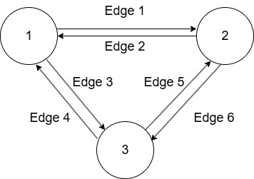
GNNs operate on graphs by utilizing nodes and edges where the nodes represent entities and edges denote the interactions between these entities. Through techniques like message passing, nodes update their states based on the information from their neighbors, allowing GNNs to learn and generalize from the graph structure efficiently [29,30]. This process is particularly advantageous for tasks that involve rich relational data. The motivation for applying GNNs to sea ice modeling is supported by other proven successes in similarly complex systems in other scientific domains [26][27][28]. Given these capabilities, the application of GNNs to sea ice modeling presents a promising new avenue. GNNs could capture more insights by conceptualizing sea ice dynamics into graphs, where nodes represent sea ice features, including position and velocity, and edges capture interactions such as collisions.

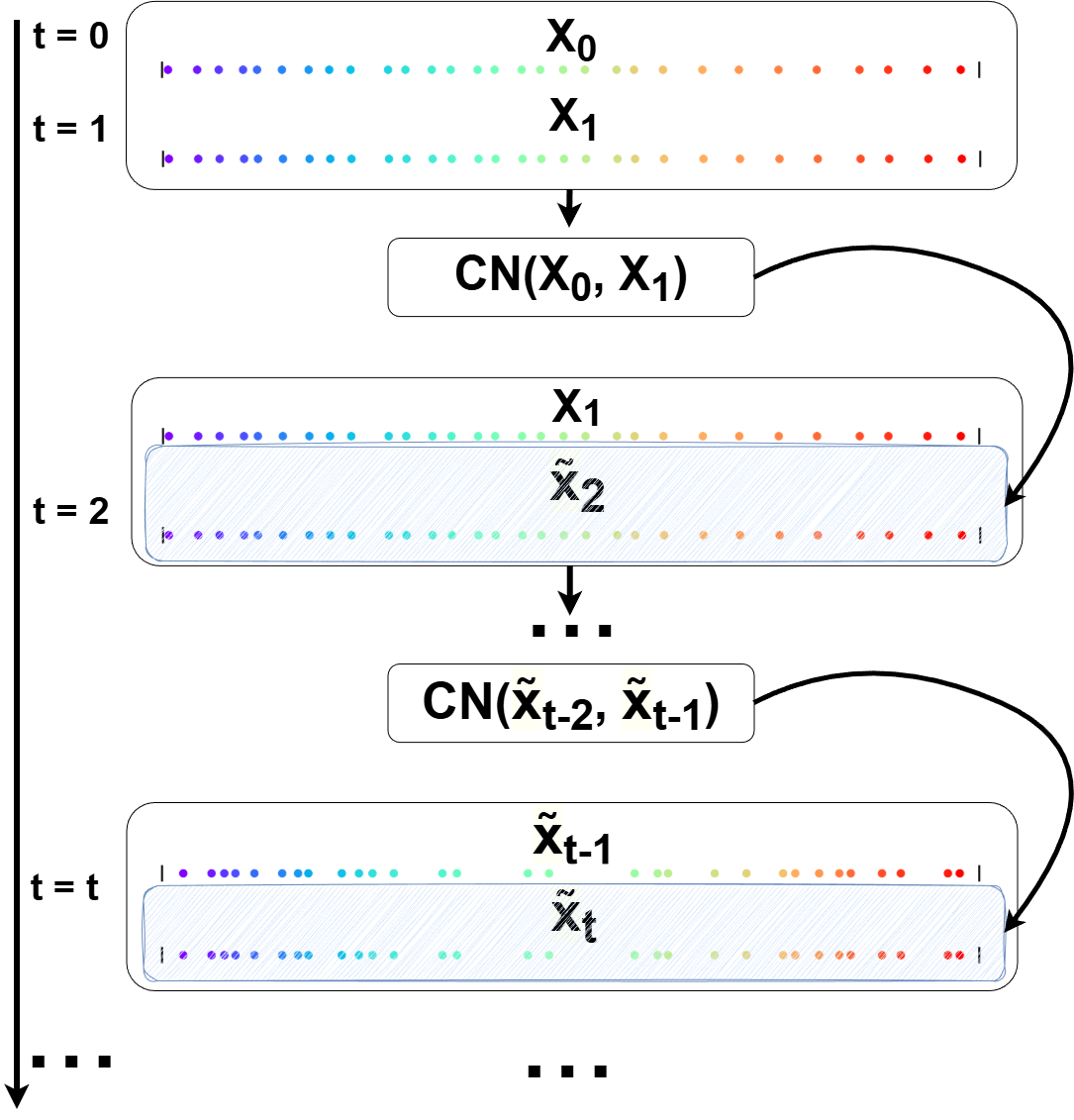
Previous efforts to simulate sea ice dynamics within the MIZ have predominantly employed Discrete Element Methods (DEM), focusing on the physical interactions of individual ice floes. These methods, while detailed, are computationally intensive and often struggle to scale up due to their high computational demands [5,22]. Surprisingly, despite the rapid advancement in machine learning technologies [31][32][33][34], there has been a noticeable absence of research exploring the use of neural networks for sea ice simulation in the MIZ. This study contributes to this area by introducing a GNN-based sea ice simulation model: proposed Collision-captured Network (CN) as Figure 1 coupled with data assimilation (DA) techniques, inspired by the Interaction Network [35]. By leveraging the inherent graph structure of sea ice interactions in the MIZ, the proposed model offers an innovative solution that reduces computational overhead while

…(Full text truncated)…