A Rough Functional Breuer-Major Theorem

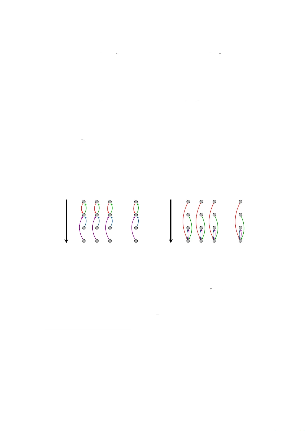
A Rough F unctional Breuer–Ma jor Theorem Henri Elad Altman, T om Klose, Nicolas P erk o wski F ebruary 19, 2026 Abstract W e extend the functional Breuer–Major theorem b y Nourdin and Nualart (2020) to the space of rough paths. The pro of of tightness combines the m ultiplication formula for iterated Mallia vin div ergences, due to F urlan and Gubinelli (2019), with Mey er’s inequalit y and a K olmogorov-t ype criterion for the r -v ariation of càdlàg rough paths, due to Chevyrev et al. (2022). Since martingale techniques do not apply , we obtain the conv ergence of the ﬁnite-dimensional distributions through a b esp ok e v ersion of Slutsky’s lemma: First, we o vercome the lac k of hypercontractivit y by an iterated in tegration-by-parts scheme which reduces the remaining analysis to ﬁnite Wiener c haos; crucially , this argument relies on Malliavin diﬀerentiabilit y of the nonlinearity but not on c haos deca y and, as a consequence, encompasses the centred absolute v alue function. Second, in the spirit of the la w of large n umbers, we show that the diagonal of the second-order pro cess conv erges to an explicit symmetric correction term. Finally , w e compute all the moments of the remaining process and, through a ﬁne com binatorial analysis, sho w that they conv erge to those of the Stratono vic h Bro wnian rough path p erturb ed b y an an tisymmetric area correction, as computed b y a suitable amendment of F aw cett’s theorem. All of these steps b eneﬁt from a ma jor combinatorial reduction that is implied b y the original argument of Breuer and Ma jor (1983). K ey wor ds and phr ases. Breuer–Ma jor theorem, Rough paths, Rough inv ariance principles, Malliavin calculus, Mey er’s inequality , Hermite shift 2020 Mathematics Subje ct Classiﬁc ation. 60F17, 60L20, 60H07 Con ten ts 1 In tro duction 2 2 Preliminaries and auxiliary results 12 2.1 Notation . . . . . . . . . . . . . . . . . . . . . . . . . . . . . . . . . . . . . 12 1 2.2 Mallia vin calculus . . . . . . . . . . . . . . . . . . . . . . . . . . . . . . . 13 2.3 The Hermite shift op erator . . . . . . . . . . . . . . . . . . . . . . . . . . 17 2.4 Diagram formula, regular, and irregular diagrams . . . . . . . . . . . . . . 18 2.5 Con vergence of normalised sums of cov ariances . . . . . . . . . . . . . . . 22 3 Tigh tness 23 3.1 V ariation top ologies on rough paths . . . . . . . . . . . . . . . . . . . . . 23 3.2 Tigh tness result . . . . . . . . . . . . . . . . . . . . . . . . . . . . . . . . . 25 3.3 Pro of of moment estimates for tigh tness . . . . . . . . . . . . . . . . . . . 27 4 Con v ergence of ﬁnite-dimensional distributions 33 4.1 Ov erview and strategy . . . . . . . . . . . . . . . . . . . . . . . . . . . . . 34 4.2 Reduction to ﬁnite chaos . . . . . . . . . . . . . . . . . . . . . . . . . . . . 40 4.3 A law of large num bers on the diagonal . . . . . . . . . . . . . . . . . . . 54 4.4 Momen t computations . . . . . . . . . . . . . . . . . . . . . . . . . . . . . 56 4.4.1 Relation to moment con v ergence . . . . . . . . . . . . . . . . . . . 60 4.4.2 Higher-order diagonals v anish . . . . . . . . . . . . . . . . . . . . . 64 4.4.3 Analysis of pairings . . . . . . . . . . . . . . . . . . . . . . . . . . 71 4.4.4 Con vergence of momen ts . . . . . . . . . . . . . . . . . . . . . . . . 76 4.5 Remo ving the chaos cut-oﬀ . . . . . . . . . . . . . . . . . . . . . . . . . . 79 4.6 Pro of of Theorem 4.1 . . . . . . . . . . . . . . . . . . . . . . . . . . . . . . 81 A Mo diﬁcations to the pro of b y Breuer and Ma jor 81 B T echnical pro ofs 83 B.1 Pro of that non-ladder pairings v anish . . . . . . . . . . . . . . . . . . . . 83 B.2 Pro of that cross-simplex pairings v anish . . . . . . . . . . . . . . . . . . . 89 C Coun terexample to the conditional decay condition 89 References 92 1 In tro duction The Centr al Limit The or em (CL T) is at the heart of probabilit y and statistics. W e can state it in the follo wing wa y: for a sequence of cen tred i.i.d. random v ariables Z = ( Z i ) i ∈ Z with v ariance σ 2 Z < ∞ , there exists an i.i.d. sequence of standard normal Gaussians X = ( X i ) i ∈ Z and a real-v alued function 1 f such that Z i d = f ( X i ) and 1 N 1 / 2 N − 1 X i =0 f ( X i ) − → N (0 , σ 2 Z ) in la w as N → ∞ . 1 F or example, one can take f = F − 1 Z ◦ Φ where F − 1 Z is the quantile function of Z and Φ the standard normal cumulativ e distribution function. 2 In many applications of interest, ho w ever, the data exhibits non-trivial c orr elations (see, for example, [Ber92] for a v ariety of examples) and th us violates the crucial indep endence assumption. In this context, the celebrated Breuer–Ma jor theorem [BM83] pro vides a suﬃcien t criterion on the fu nction f and the decay of correlations under which one can still observe CL T b eha viour: Theorem 1.1 (Breuer–Ma jor) Consider a stationary se quenc e X = ( X i ) i ∈ Z of c en- tr e d, one-dimensional Gaussian r andom variables with c ovarianc e function ρ ( i ) = E [ X 0 X i ] such that ρ (0) = 1 . F urther, let γ : = N (0 , 1) and f ∈ L 2 ( γ ) with Hermite r ank d ≥ 1 , i.e. its chaos de c omp osition is given by f ( x ) = ∞ X q = d c q H q ( x ) wher e H q denotes the q -th Hermite p olynomial. Then, if ρ ∈ ℓ d ( Z ) and S N is given by S N ( t ) : = 1 N 1 / 2 ⌊ N t ⌋− 1 X i =0 f ( X i ) , t ∈ [0 , 1] , we have S N f.d.d. − → σ B as N → ∞ (1.1) wher e B is a standar d Br ownian motion and the varianc e σ 2 is given by σ 2 : = ∞ X q = d q ! c 2 q X k ∈ Z ρ ( k ) q < ∞ . (1.2) The previous theorem immediately b egs the question as to whether the conv ergence in (1.1) can b e up dated to functional c onver genc e in the Skorokhod space D (0 , 1) . As Cham b ers and Slud [CS89] hav e shown b y an explicit counterexample, this is not the case under the sole assumptions that f has Hermite rank d and ρ ∈ ℓ d ( Z ) ; instead, they pro vide a suﬃcient condition, later sligh tly improv ed by Ben Hariz [BH02], whic h requires explicit information on the decay of the Hermite co eﬃcients ( c q ) q ≥ d . Their fast chaos de c ay assumption , ho w ever, is diﬃcult to v erify in practice and has been replaced by Nourdin and Nualart [NN20] (see also their joint w ork with Campese [CNN20]) b y the less restrictive, more easily chec kable assumption that f ∈ L p 1 ( γ ) for some p 1 > 2 . Main result. The purp ose of the present w ork is to lift the functional Breuer–Ma jor theorem to the space of r ough p aths whic h, in order to b e non-trivial, requires to lo ok at R m -v alued functions  f for m ≥ 2 . More precisely , w e consider the vector of functions  f = ( f 1 , . . . , f m ) , f k : R → R , 3 where eac h f k ∈ L 2 ( γ ) is of the same ﬁnite Hermite rank d ≥ 1 with corresponding Hermite decomp osition f k ( x ) = X q ≥ d c ( k ) q H q ( x ) , k ∈ J 1 , m K : = { 1 , . . . , m } . (1.3) In addition, from here onw ards, we let ( X i = ( X (1) i , . . . , X ( m ) i )) i ∈ Z (1.4) b e an R m -v alued stationary centred Gaussian sequence, that is, a m ultiv ariate Gaussian pro cess indexed by Z . In addition, for k , ℓ ∈ J 1 , m K , w e let 2 ρ k,ℓ ( j − i ) : = E [ X ( k ) i X ( ℓ ) j ] (1.5) and assume that ρ k,k (0) = 1 . Note that ρ k,ℓ ( u ) = ρ ℓ,k ( − u ) for u ∈ Z . F or t ∈ [0 , 1] , w e then deﬁne S N ( t ) = ( S N ( t ) , S N ( t )) where the ﬁrst and se c ond-or der pr o c esses S N and S N are, resp ectively , given b y S N ( t ) : = 1 N 1 / 2 ⌊ N t ⌋− 1 X i =0  f ( X i ) , S N ( t ) : = 1 N X 0 ≤ i 2 we have lim N →∞ S N = B in law in D r − var ([0 , 1]; R m ) (1.8) 2 Observ e that, by c onvention , we alwa ys write ρ k,ℓ ( n ) to denote the time diﬀerence from the ﬁrst to the second v ariable enco ded by the subindices, and not the other w ay round. 3 See Remark 1.5 b elow for further comments. 4 W e in tro duce the parameter p here, so we can later refer to it. 4 wher e B = ( B , B ) is a Br ownian r ough p ath with char acteristics (Σ , Γ) , that is: (i) The ﬁrst c omp onent B is an m -dimensional Br ownian motion with c ovarianc e matrix Σ given by Σ = D + 2 Sym (Γ) (1.9) wher e ∆( u ) : = E h  f ( X 1 ) ⊗  f ( X u +1 ) i , i.e. ∆ k,ℓ ( u ) = X q ≥ d q ! c ( k ) q c ( ℓ ) q ρ k,ℓ ( u ) q (1.10) and D as wel l as Γ ar e given by D : = ∆(0) , Γ : = ∞ X u =1 ∆( u ) . (1.11) (ii) The se c ond c omp onent B is of the form B ( t ) = Z t 0 B ( s ) ⊗ d B ( s ) + t Γ , (1.12) wher e the inte gr ation denotes Itô integration , cf. R emark 1.4, Point (iv) b elow. W e record the follo wing corollary which is an immediate consequence of the contin uit y of the Itô–Lyons map w.r.t. rough paths metric in D r − var ([0 , 1]; R m ) , see [CFK + 22, Coro. 4.4]. Recall that  f ( X i ) has b een introduced in (1.7). Corollary 1.3 L et n, N ≥ 1 and r > 2 . F or b ∈ C 3 b ( R n ; R n ) and V ∈ C 3 b ( R n ; R n × m ) , let Y N b e deﬁne d thr ough the Euler-typ e r e curr enc e r elation Y N  i + 1 N  = Y N  i N  + 1 √ N V  Y N  i N   f ( X i ) + 1 N b  Y N  i N  , Y N (0) = y N ∈ R n , whenever i ∈ J 0 , N − 1 K , which is extende d to t ∈ [0 , 1] by setting Y N ( t ) : = Y N  i N  whenever i/ N ≤ t < ( i + 1) / N . F or Γ ∈ R m × m given in (1.11) , deﬁne c : R n → R n thr ough c ( z ) : = m X k,ℓ =1 Γ k,ℓ [( V k · ∇ ) V ℓ ] ( z ) , [( V k · ∇ ) V ℓ ] j ( z ) : = n X u =1 ∂ V j,ℓ ( z ) ∂ z u V u,k ( z ) , j ∈ J 1 , n K . If y N → y as N → ∞ , then Y N c onver ges in law in r -variation top olo gy to the unique str ong solution of the SDE d Y ( t ) = V ( Y ( t )) d B ( t ) + [ b ( Y ( t )) + c ( Y ( t ))] d t, Y (0) = y , wher e B is an R m -value d Br ownian motion with c ovarianc e matrix Σ (at time 1 ) given in (1.9) . 5 Before we discuss how the previous theorem relates to the existing literature, a few remarks are in order. Remark 1.4 (General commen ts) (i) The pr evious r esult also holds for p > 1 and d ∈ { 1 , 2 } , i.e. under less stringent in- te gr ability, but mor e stringent summability assumptions. Se e R emark 1.5, Point (iii) and, in p articular, R emark 4.28 for mor e detaile d c omments in this dir e ction. (ii) The pr evious the or em cannot b e de duc e d fr om any mixing-typ e c onditions. In fact, Br euer and Major [BM83] have alr e ady pr ovide d two explicit se quenc es of r andom variables which gener ate the same σ -algebr a, but one of them ob eys the CL T while the other satisﬁes a non-central limit theorem in the spirit of Dobrushin and Major [DM79, Maj81], R osenblatt [R os81], and T aqqu [T aq75, T aq77, T aq79]. (iii) The assumption that al l functions f k have the same Hermite r ank at le ast d c an e asily b e dr opp e d: If we denote by d k ≥ 1 the lower b ound for the Hermite r ank of f k , then al l the ar guments in this article work for d : = min k =1 ,...,m d k . (iv) The fact that B c an only have char acteristics (Σ , Γ) given in (1.9) and (1.11) , r esp e ctively, is wel l-understo of by now, cf. [EFO24, Thm. 1]; the diﬃculty lies in the veriﬁc ation of its pr er e quisities which ar e a sp e cial c ase of our c omputations in Se ction 4. Note that, sinc e we c an de c omp ose Γ into symmetric and antisymmetric p art, Γ = Sym(Γ) + A , A : = ASym(Γ) (1.13) the formula for Σ in (1.9) c ombine d with Itô–Str atonovich c orr e ction implies that B ( t ) = Z t 0 B ( s ) ⊗ ◦ d B ( s ) − t 2 D + t A , (1.14) wher e ◦ denotes Stratono vich in tegration . While the natur al exp e cte d limit is given by the Itô lift of B , r epr esenting B as in (1.14) is mor e aligne d with our pr o of, se e the str ate gy and or ganisation p ar agr aphs b elow. (v) L et us c omment on the structur al assumption in (1.7) . In line with the work by A r c ones [A r c94], the most gener al assumption would b e for the pr o c ess X in (1.4) to b e an R n -value d, c entr e d, and stationary Gaussian pr o c ess for some n ∈ N such that e ach function f k : R n → R has X as its input, i.e. f k ( X i ) = f k ( X (1) i , . . . , X ( n ) i ) . However, this would le ad to a signiﬁc ant incr e ase in notation c omplexity (for example due to multivariate Hermite exp ansions) without adding much c onc eptual value. In c ontr ast, our “diagonal c ase” in (1.7) gives non-trivial symmetric and area corrections D and A without b eing overly notational ly involve d; we exp e ct our ar guments for that c ase to gener alise without much diﬃculty. 6 (vi) Observe that the univ ariate case , i.e. if ( X i ) i ∈ Z is a one-dimensional stationary Gaussian se quenc e as in The or em 1.1, is a sp e cial (de gener ate) c ase in which ( X (1) i , . . . , X ( m ) i ) = ( X i , . . . , X i ) . In this sc enario, we wil l simply write ρ inste ad of ρ 1 , 1 and note that ρ ( u ) = ρ ( − u ) which, in turn, implies that A ≡ 0 and Γ = Sym(Γ) . Remark 1.5 (Diﬀerentiabilit y , in tegrabilit y , and summability assumptions) (i) Diﬀer entiability. The Mal liavin–Sob olev r e gularity assumption (1) is crucial in two plac es, namely in the pr o of of the tightness estimate (The or em 3.4) and in the reduction to ﬁnite chaos (Pr op osition 4.10) for the f.d.d. c onver genc e. In b oth c ases, the r e ason for the incr e ase d r e gularity (as c omp ar e d to the ﬁrst-level c ase by Nour din and Nual art [NN20]) is the same: While the d -th Hermite shift (se e Deﬁnition 2.18) incr e ases r e gularity by d , by the L eibniz rule, the 2 d Mal liavin derivatives enc o de d in the pr o duct might al l hit the same of the two factors, thus le ading to d r e quir e d derivatives for e ach of the factors. W e do not know whether the r esulting assumption on the Mal liavin diﬀer entiability is optimal or an artefact of our pr o of. (ii) Summability. F or il lustr ational purp oses, supp ose for a moment that we ar e in the univer ate setting of R emark 1.4, Point (vi). A s we have just discusse d in Point (i), our ar gument r e quir es d Mal liavin deriva- tives to work. Note that ther e is a fundamental tension b etwe en this (enc o de d by assumption (1) in The or em 1.2) and assumption (2): While the latter b e c omes a stronger r e quir ement when d shrinks, the former b e c omes w eak er , and vic e versa. In fact, this observation is the r e ason why The or em 1.2 is phr ase d so as to r e quir e Hermite r ank “at le ast” d ≥ 1 b e c ause the Hermite r ank is not str aightforwar d ly c onne cte d to the or der of Mal liavin diﬀer entiability. A p ar adigmatic example is the c entr e d absol ute value function f ( x ) = | x | − r 2 π which has Hermite r ank 2 but f / ∈ D 2 ,q ( γ ) for any q . However, cho osing d = 1 , we do know that f ∈ D 1 ,q ( γ ) for al l q —it is, ther efor e, c over e d by our assumptions pr ovide d we have ρ ∈ ℓ 1 ( Z ) (inste ad of just ρ ∈ ℓ 2 ( Z ) ). In addition, note that imp osing that f = f k has “at le ast” Hermite r ank d is c onsistent with The or em 1.1. Inde e d: If f had Hermite r ank d ⋆ ≥ d and we did imp ose ρ ∈ ℓ d ( Z ) , then ρ would also b e in ℓ d ⋆ ( Z ) and the c onclusion of the the or em holds. In that (simpler) setting, ther e is just nothing to b e gaine d fr om this tr ade-oﬀ. (iii) Inte gr ability. The p ar ameter p ≥ 2 in the Mal liavin–Sob olev r e gularity assump- tion (1) c orr esp onds to p 1 in the work by Nour din and Nualart [NN20], i.e. p 1 = 2 p . W e r e c al l that they only de al with the ﬁrst-or der pr o c ess S N in (1.6) and r e quir e p 1 > 2 7 to obtain functional c onver genc e. Ther efor e, the natur al assumption for us should b e p > 1 (for tightness) and p = 1 (for the f.d.d. c onver genc e). F or tightness , assuming p > 1 se ems inde e d to b e enough: W e pr ovide detaile d c omments in R emark 3.8. F or the f.d.d. conv ergence (The or em 4.1), in c ontr ast, p = 2 is crucial. This is de eply c onne cte d with the br e akdown of Meyer’s ine quality for p = 1 and the fact that the Poinc ar é ine quality c an only c omp ensate for it when d ∈ { 1 , 2 } in (1); this has alr e ady b e en observe d by A ddona, Mur atori, and R ossi [AMR22]. W e pr ovide detaile d c omments in R emarks 4.5 and 4.7 b elow. A s a c onse quenc e, we ne e d to c ontr ol the L 2 ( P ) -norm (and not just that in L 1 ( P ) ) of S N in Pr op osition 4.10. L et us also mention that this is structur al ly similar to a pr oblem in quantitative Br euer–Major the or ems: While Nour din, Nualart, and Pe c c ati [NNP21] (whose str ate gy informs p arts of our ar gument) r e quir e f k ∈ D 1 , 4 ( γ ) and d = 2 , A ngst, Dalmao, and Poly [ADP24] have r e c ently shown that f k ∈ D 1 , 2 ( γ ) is enough by me ans of the so-c al le d sharp op er ator. It would b e very inter esting to se e if those te chniques would also apply in our c ontext. (iv) Pr oje ction. After pr oje ction to ﬁnite chaoses of or der less than or e qual to M in Se ction 4.2, the functions f M k ar e Mal liavin smo oth and have moments of al l or ders; ac c or dingly, Se ctions 4.3 and 4.4 only r e quir e the assumption ρ k,ℓ ∈ ℓ d ( Z ) via the summability ∆ M ∈ ℓ 1 ( Z ) (for ∆ as in (1.10) and ∆ M its c ounterp art with al l functions f k pr oje cte d onto chaos c omp onents M and lower). Discussion and relation to the literature. Theorem 1.2 ﬁts squarely in to an ever gro wing b o dy of literature on r ough invarianc e principles , comprising the rough Donsker’s theorem [BFH09], magnetic Bro wnian motion [FGL15], slo w-fast systems [KM16, KM17, CFK + 19, CFK + 22], random w alks in random en vironment [DOP21, Ore21, LO21], as w ell as av eraging [FK24] and rough (fractional) homogenisation [GL22, GL20, GLS22, HL20, HL23, DKP25]; w e refer to the recent article [EF O24] for a systematic and more complete o verview based on the Green–Kub o formula. F undamen tally , the diﬃculty in establishing Theorem 1.2 is t w o-fold: (1) Eac h of the functions f k in (1.3) is allo wed to ha ve an inﬁnite chaos de c omp osition , whic h rules out arguments based on Gaussian hypercontractivit y . This is particularly relev ant since computing p -th moments of the pro cess S N for p ≥ 2 is similar to computing (2 p ) -th moments of the functions f k but it is kno wn that c haos tails do not generally decay in an y other space than L 2 . (2) The sequence ( X i ) i ∈ Z has non-trivial c orr elations , whic h prohibits the use of mar- tingale tec hniques to sho w conv ergence in ﬁnite-dimensional distributions to the limiting rough path. Although viewed from a homogenisation p ersp ective sligh tly diﬀerent from ours, similar problems ha ve app eared in the w ork of Gehringer and Li [GL22, GL20] and their join t 8 w ork with Sieb er [GLS22], so w e will now discuss in which wa y our w ork diﬀers from theirs. First, let us mention that they deal with the mixe d c ase where some of the comp onen ts f k enjo y the CL T scaling, while others ob ey a non-central CL T scaling that leads to Hermite pro cesses in the limit; crucially , the latter are not momen t-determined in general, whic h complicates the conv ergence analysis. How ev er, while the mixed case is v ery interesting from a mo delling p ersp ective, the iterated integrals become Y oung inte gr als if at least one of the inv olv ed comp onents is of Hermite type. F rom now on w ards, we will therefore fo cus on the pur ely Gaussian part of their work (with truly rough limits), sp eciﬁcally w.r.t. the t w o issues raised ab ov e and phrased in the terminology of the article at hand. (1) In case f k has comp onents in inﬁnitely many c haoses, [GL22, GL20, GLS22] imp os e a fast chaos de c ay assumption akin to that of Chambers and Slud mentioned ab ov e. In essence, this assumption guaran tees that one can obtain the required L 2 p -estimates for p > 2 , whic h are necessary for tightness, by Gaussian hypercontractivit y . Ho wev er, that assumption is systematic al ly str onger than our assumption that f k ∈ D d, 2 p ( γ ) . In particular, as pointed out b y Nourdin and Nualart [NN20], it do es not cov er the b enchmark case f k ( x ) = | x | − p 2 / π while ours do es, alb eit at the price of the stronger assumption that ρ ∈ ℓ 1 ( Z ) , see Remark 1.5 for details. (2) In order to establish the con v ergence in ﬁnite-dimensional distributions, [GL22, GL20, GLS22] imp ose a c onditional de c ay c ondition on the functions f k w.r.t. the Gaussian sequence X = ( X i ) i ∈ Z . Giv en this assumption, they can again resort to martingale tec hniques to sho w the conv ergence of the ﬁnite-dimensional distributions. Ho wev er, w e will see in Appendix C that, already in the univ ariate setting of Remark 1.4 (vi), there is a ric h family of long-r ange dep endent stationary Gaussian sequences X (i.e. ρ / ∈ ℓ 1 ( Z ) ) such that the function f k = H d for some d ≥ 2 violates the conditional deca y assumption w.r.t. X . In contrast, w e will show that ρ ∈ ℓ d ( Z ) such that the coun terexample is, indeed, cov ered by our main result. On the one hand, our tightness argument uses more ﬂexible Mallia vin calculus tools (rather than moment-computations com bined with the fast c haos deca y condition). On the other hand, in our case, the limit is momen t-determined and w e develop a nov el reduction argumen t for the f.d.d. conv ergence, based on in tegration-by-parts, that comp ensates the lac k of martingale metho ds. W e will pro vide further details in the strategy paragraph b elo w. Before doing s o, w e wan t to highligh t that the problem of a nonlinearity with comp onents in inﬁnitely many chaoses is also an active research direction in the study of (singular) sto c hastic partial diﬀeren tial equations, see [GP16, FG19, HX19] in the Gaussian and [KWX24] in the P oisson case. While these works deal with so-called subcritical equations and in the w eak coupling regime, the recent w ork of Cannizzaro, the second named author, and Moulard [CKM26] has, for the ﬁrst time, tackled this problem in case of the critic al Stochastic Burgers Equation with general nonlinearity , b oth on the full space and at strong coupling. Finally , let us men tion that the tec hniques dev elop ed in the abov e-men tioned works hav e recen tly b een employ ed b y Kong and W ang [KW25] to pro v e the functional Breuer–Ma jor 9 theorem in the Poisson case, in which Meyer’s inequalit y is not av ailable. Strategy of proof, k ey no v elties, and insigh ts. In order to establish Theorem 1.2, w e need to show tigh tness and conv ergence of the ﬁnite-dimensional distributions. (1) Tightness : As for Nourdin and Nualart, the key tools for establishing tigh tness will come from Malliavin calculus, namely the regularisation prop erties of the Hermite shift operator alongside Meyer’s inequalities for iterated div ergences. In contrast to their work, ho w ev er, the second-order pro cess S k,ℓ N in volv es the pr o duct of f k ( X ( k ) i ) and f ℓ ( X ( j ) j ) . Representing both as iterated Mallia vin divergences with input the resp ectiv e Hermite shifts, the key no v elty is our use of multiplic ation formula for iter ate d diver genc es due to F urlan and Gubinelli [FG19], see Prop osition 2.10 below. As w e will see, the multiplication form ula includes up to 2 d Mallia vin deriv ativ es of the d -th Hermite shift of f k and f ℓ , i.e. d deriv atives on f k and f ℓ itself, cf. Remark 1.5, Poin t (i). (2) Conver genc e of ﬁnite-dimensional distributions : Modern pro ofs of the Breuer– Ma jor theorem, for example in [NP12, Chap. 7], make use of the Mallia vin–Stein metho d; in turn, ho w ev er, this requires a go o d enough understanding of the limiting distribution. In contrast to the Gaussian case (related to the ﬁrst rough path lev el B ), this is not av ailable for the second-order pro cess B . In the absence of martingale argumen ts, the sa ving grace is that ( B ( s, t ) , B ( s, t )) ∈ R ⊗ m ⊕ ( R m ) ⊗ 2 is in the second (inhomogeneous) Wiener chaos and, thereby , its la w is momen t- determined. In computations structurally similar to those of Hairer [Hai25], we therefore show con v ergence of all the moments. The argumen t is quite in tricate, so w e will present a detailed outline of the strategy in Section 4.1 b elow and just summarise the key diﬃculties and insigh ts here: ⋆ When computing exp ectations of pro ducts of terms f w j ( X ( w j ) i j ) , w j ∈ J 1 , m K for j ∈ J 1 , l K and l ≥ 2 , the Breuer–Ma jor argumen t (see Proposition 2.29 b elo w for a recap) still applies in the m ultiv ariate setting and if there are constrain ts b et ween the indices i 1 , . . . , i l : It states that, asymptotic al ly , Wick’s theorem applies, leading to a ma jor computational simpliﬁcation. The reason is that the argumen t by Breuer and Ma jor do es not use the sign of the correlations ρ k,ℓ . ⋆ Chaos tails do not decay in L p for p > 2 . As a consequence, lo oking at S k,ℓ N as deﬁned in (1.6) but with at least one of the functions f k and f ℓ pro jected on to c haoses M and higher, it is not at all clear ho w to show that its L 2 -norm (i.e., morally , the L 4 -norm of f k and f ℓ !) go es to zero as M tends to inﬁnit y . Instead of h yp ercontractivit y , we will use an iterated Gaussian in tegration-by- parts pro cedure, the computational complexity of which w e tame by a graphical notation similar to F eynman diagrams (in the sense of pairwise matchings); this allo ws to split the expression for ∥ S k,ℓ N ∥ L 2 in to a deterministic and (an exp ectation of ) a pr ob abilistic part. Roughly sp eaking, in most cases, the deterministic part will v anish as N → ∞ while the probabilistic part is independent of N 10 and uniformly b ounded in the m ulti-index for eac h ﬁxed M , thanks to the diﬀeren tiability assumption (1) in Theorem 1.2. In the few other cases, the deterministic part is uniformly b ounded in N while the probabilistic part v anishes as M → ∞ . W e refer to the paragraph on p. 42 for details. ⋆ It is precisely the “diagonal terms”, corresp onding to i = j in (1.6) , that asymp- totically give the D in (1.14) , i.e. the symmetric part of correction to the Str atonovich Br ownian r ough p ath . W e will see that this is a relativ ely straight- forw ard consequence of the original Breuer–Ma jor argument. ⋆ A dding the diagonals (times a factor (1 / 2) ) to S N in (1.6) , w e can temp orarily con vert from the piecewise constan t to the piecewise linear interpolation. In this wa y , w e can use iterated inte gr al -signatures and b ypass the need to work with iterated sum-signatures as dev elop ed and inv estigated b y [KO19, DEFT20b, DEFT20a, DEFT23] in the context of mac hine learning and time series analysis (see Remark 4.23 for further comments in this direction). As indicated in (1.14) , our momen t computations then need to repro duce those of the Stratono vic h rough path, shifted by the an tisymmetric matrix A , in the limit. ⋆ In the detailed conv ergence analysis for the momen ts of S N with the diagonals added in, w e will iden tify the exact mechanism that gives rise to the A -translated Stratono vich signature of Brownian motion. More precisely: (1) Odd tensor comp onen ts v anish b ecause, in the language of Breuer and Ma jor, there are no regular diagrams with an o dd n um b er of lev els. (2) In the “asymptotic Wic k theorem” implied by their argumen t, at tensor lev el 2 n , only the ladder pairing P ⋆ = {{ 1 , 2 } , { 3 , 4 } , . . . , { 2 n − 1 , 2 n }} surviv es in the limit. (3) Not all m ulti-indices 0 ≤ i 1 ≤ . . . ≤ i 2 n ≤ N − 1 con tribute to that limit. In fact, “diagonals of order 3 and higher” (i.e. when three or more consecutiv e indices coincide) v anish as ymptotically . (4) F urther, equality betw een t w o consecutive indices is only asymptotically relev an t if it is in accordance with the pairing P ⋆ , i.e. 0 ≤ i 1 ≤ i 2 < i 3 ≤ i 4 < . . . < i 2 n − 1 ≤ i 2 n . (5) Sums ov er equal indices giv e rise to 1 2 ∆(0) = 1 2 D and, otherwise, to Γ = P k ∈ N ∆( k ) . This com bines to 1 2 D + Γ = 1 2 (Σ + 2 A ) , as implied by a suitable amendment of F aw cett’s theorem. Organisation of the article. The remainder of the article is organised as follows. In Section 2, we introduce some notation and recall basic concepts of Gaussian analysis and Mallia vin calculus. In particular, we recall the original argumen t by Breuer and Ma jor and precisely state the form in which w e use it throughout the article (Corollary 2.31). In Section 3, we brieﬂy recall bac kground material on rough path spaces equipp ed with r -v ariation top ologies (Section 3.1) and, in Section 3.2, then establish tightness in suc h spaces (Corollary 3.6); the key L p -estimates are presen ted in Theorem 3.4 and prov ed in Section 3.3. Section 4 establishes th e conv ergence of the ﬁnite-dimensional distributions (Theorem 4.1). W e b egin with a high-level o v erview of the strategy in Section 4.1 whic h leads to the tailor-made Slutsky-type statement (Prop osition 4.2) that the ensuing analysis is based up on. W e then implemen t the outlined agenda b y verifying the assumptions for the Slutsky-type result in the sections that follow. Section 4.2 con tains the reduction 11 step which sho ws that c haos tails ab ov e a ﬁxed order v anish asymptotically in a suitable double limit. As a consequence, w e can alw ays assume that we are w orking in a ﬁxed (inhomogeneous) chaos. In Section 4.3, we then show that, in the spirit of the la w of large n umbers, the diagonals of order tw o give rise to the term D in (1.14) . Section 4.4 contains a detailed combinatorial analysis, as outlined in the strategy paragraph, culminating in the pro of of Theorem 4.24 (via that of Theorem 4.29), whic h shows that the momen ts of the discrete appro ximation conv erge to those of the Stratono vich rough path corrected b y A . In Section 4.5, we then remo v e the chaos cut-oﬀ in tro duced in Section 4.2 from the limiting rough path, whic h only enters via the cov ariance matrix and the corrections. Finally , in Section 4.6, we bring all the previous eﬀort to fruition and presen t the pro of of Theorem 4.1 which establishes the f.d.d. conv ergence. A c kno wledgemen ts. W e are grateful to Ilya Chevyrev, Emilio F errucci, F anhao Kong, Iv an Nourdin, Nik olas T apia, and W eijun Xu for insigh tful discussions that ha ve b eneﬁted this work. W ork on this pro ject started as HEA w as b eing employ ed as Dirichlet P ostdoctoral F ello w in Mathematics at F reie Univ ersität Berlin, with funding provided b y MA TH+, in the framew ork of the “MA TH+ EXC 2046” research project. TK is supp orted by a UKRI Horizon Europ e Guaran tee MSCA P ostdo ctoral F ellowship (UKRI, SPDEQFT, gran t reference EP/Y028090/1). Views and opinions expressed are ho wev er those of the authors only and do not necessarily reﬂect those of UKRI. In particular, UKRI cannot b e held resp onsible for them. NP gratefully ac knowledges funding b y the Deutsche F orsch ungsgemeinsc haft (DFG, German Research F oundation) – CR C/TRR 388 “Rough Analysis, Sto chastic Dynamics and Related Fields” – Pro ject ID 516748464 2 Preliminaries and auxiliary results In this section, we collect preliminaries and auxiliary results that will be used throughout the article. 2.1 Notation • F or tw o expressions A and B , we write A ≲ B if there exists a constant c > 0 such that A ≤ cB . If the constan t c dep ends on a parameter α , we will write A ≲ α B . • W e write N for the natural num bers starting from 1 and N 0 : = N ∪ { 0 } . F or a, b ∈ R suc h that a < b , w e write J a, b K : = [ a, b ] ∩ Z . • W e write A N ≍ B N if A N = B N + o (1) as N → ∞ , i.e. lim N →∞ A N = lim N →∞ B N . Unless otherwise stated, w e will exclusiv ely use this notation for the limit N → ∞ whic h is particularly relev an t for quantities dep ending, additionally , on another parameters b esides N . 12 • F or k ∈ N , we use the multi-index notation i 1 : k : = ( i 1 , . . . , i k ) and i [1 : k ] : = P k j =1 i j . F urthermore, for a, b ∈ R suc h that a < b , w e write a ≤ i 1 : k ≤ b to mean a ≤ i ℓ ≤ b for all ℓ ∈ J 1 , k K . • F or l ∈ N , we let □ l,N : = J 0 , N − 1 K l denote the l -dim. b o x of side length N − 1 . • F or l ∈ N and a, b ∈ Z with a < b , we let △ ( l ) a,b : = n r 1 : l ∈ [ a, b ] l : a ≤ r 1 < r 2 < . . . < r l ≤ b − 1 o denote the l -dim. simplex o ver the in terv al [ a, b ] as w ell as its closure ¯ △ ( l ) a,b = n r 1 : l ∈ [ a, b ] l : a ≤ r 1 ≤ r 2 ≤ . . . ≤ r l ≤ b − 1 o W e will not notationally distinguish the discr ete simplex , i.e. the case when a, b, r 1 : ℓ in the previous deﬁnition are constrained to b e integers. 2.2 Mallia vin calculus In this section, w e introduce the key concepts and results from Malliavin calculus which w e will use throughout this article. F or a detailed introduction to these topics, we refer the reader to the b ooks b y Nualart [Nua06] and Nourdin and Peccati [NP12]. W e need the following auxiliary deﬁnition: Deﬁnition 2.1 (Isonormal Gaussian process) L et H b e a r e al sep ar able Hilb ert sp ac e. A sto chastic pr o c ess W = { W ( h ) : h ∈ H } , deﬁne d on a c omplete pr ob ability sp ac e (Ω , F , P ) , is an isonormal Gaussian pro cess over H if W is a c entr e d Gaussian family of r andom variables such that E [ W ( h ) W ( g )] = ⟨ h, g ⟩ for al l g , h ∈ H . Recall that { X i } i ∈ Z ⊆ L 2 (Ω) is a stationary sequence of cen tred, R m -v alued Gaussian random v ariables with correlation function ρ k,ℓ ( u ) = E [ X ( k ) 0 X ( ℓ ) u ] and ρ k,k (0) = 1 for all k , ℓ ∈ J 1 , m K . In particular, for any i ∈ Z and k ∈ J 1 , m K , w e hav e X ( k ) i ∼ γ for γ = N (0 , 1) . The following statemen t is a straightforw ard amendment of [NP12, Prop. 7.2.3]. Lemma 2.2 Ther e exists a r e al sep ar able Hilb ert sp ac e H , an isonormal Gaussian pr o c ess { W ( h ) : h ∈ H } over H , and a set E = { e k,i : k ∈ J 1 , m K , i ∈ Z } ⊆ H such that (i) E gener ates H , (ii) ρ k,ℓ ( j − i ) = E [ X ( k ) i X ( ℓ ) j ] = ⟨ e k,i , e ℓ,j ⟩ H for any k , l ∈ J 1 , m K and i, j ∈ Z , and (iii) X ( k ) i = W ( e k,i ) for every k ∈ J 1 , m K and i ∈ Z . 13 Deﬁnition 2.3 (Hermite p olynomials and Wiener chaos) W e let H 0 ( x ) : = 1 and, for q ∈ N , intr o duc e the q -th Hermite p olynomial H q by H q ( x ) : = ( − 1) q e x 2 2 d q d x q e − x 2 2 , (2.1) F or q ∈ N 0 , the q -th Wiener chaos W q is deﬁne d as W q : = cl L 2 (Ω) span n H q ( W ( h )) : h ∈ H , ∥ h ∥ H = 1 o . wher e cl L 2 (Ω) denotes the closur e w.r.t. L 2 (Ω) . F or the next deﬁnition, w e denote by ˜ ⊗ the symmetric tensor product on the Hilb ert space H , that is: h 1 ˜ ⊗ . . . ˜ ⊗ h q : = 1 q ! X π ∈ S ( q ) q O ℓ =1 h π ( ℓ ) . Deﬁnition 2.4 (Wiener–Itô isometry) W e let I 0 : = id R and, for q ≥ 1 , deﬁne I q : H ˜ ⊗ q → W q , I q ( h ⊗ q ) : = H q ( W ( h )) for h ∈ H, ∥ h ∥ H = 1 (2.2) which is extende d to a line ar isometry (w.r.t. the sc ale d norm √ q ! ∥·∥ H ˜ ⊗ q ). It can b e shown that an y G ∈ L 2 (Ω) admits the Wiener chaos exp ansion G = E [ G ] + ∞ X q =1 I q ( g q ) , (2.3) where the symmetric kernels g q ∈ H ˜ ⊗ q are uniquely determined by G . Deﬁnition 2.5 (Malliavin deriv ativ e) F or smo oth cylindric al r andom variables of the form G = g ( W ( h 1 ) , . . . , W ( h n )) , wher e h i ∈ H and g ∈ C ∞ b ( R n ) , the Mallia vin deriv ativ e D is deﬁne d as the H -value d r andom variable D G : = n X i =1 ∂ g ∂ x i ( W ( h 1 ) , . . . , W ( h n )) h i , i.e. D G ∈ L 2 (Ω; H ) . By iter ation, higher-or der derivatives D k G ar e deﬁne d as elements of L 2 (Ω; H ⊗ k ) and we wil l also write D 0 : = id . Deﬁnition 2.6 (Malliavin–Sobolev spaces) F or any k ∈ N 0 and p ≥ 1 , the Mallia vin– Sob olev space D k,p is obtaine d as the c ompletion of smo oth cylindric al r andom variables under the norm ∥ G ∥ p k,p : = E [ | G | p ] + k X l =1 E h ∥ D l G ∥ p H ˜ ⊗ l i . 14 Next, w e in tro duce the diver genc e op er ator δ as the adjoint of the Malliavin deriv ative D . Deﬁnition 2.7 ((Iterated) Mallia vin div ergence) W e deﬁne Dom δ : = n u ∈ L 2 (Ω; H ) : ∃ c u ∈ R , ∀ G ∈ D 1 , 2 : | E [ ⟨ D G, u ⟩ H ] | ≤ c u ∥ G ∥ L 2 (Ω) o . F or u ∈ Dom δ , the r andom variable δ ( u ) is deﬁne d via the duality r elation ∀ G ∈ D 1 , 2 : E [ Gδ ( u )] = E [ ⟨ D G, u ⟩ H ] . It is c al le d the (Malliavin) div ergence op er ator. F or k ≥ 2 , we c an analo gously deﬁne the iterated divergence op erators δ k via the duality statement ∀ G ∈ D k, 2 : E [ Gδ k ( u )] = E [ ⟨ D k G, u ⟩ H ˜ ⊗ k ] , wher e u b elongs to Dom δ k ⊆ L 2 (Ω; H ˜ ⊗ k ) . Remark 2.8 When u ∈ H ˜ ⊗ k is deterministic, we have δ k ( u ) = I k ( u ) . In p articular, this applies to u = h ⊗ k for h ∈ H . Remark 2.9 The Mal liavin derivative D and its adjoint δ have obvious analo gues for r andom variables that take values in another sep ar able Hilb ert sp ac e V , se e [NP12, Se c. 2.4 and 2.6]. If we wish to highlight this fact, we wil l for example write D k,p ( V ) etc. The c orr esp onding r esults in this subse ction then apply mutatis mutandis. Essen tially , the follo wing prop osition is the con ten t of [FG19, Lem. B.7], see also Remark 2.11 b elow. Prop osition 2.10 (Divergence multiplication formula) F or n 1 , n 2 ∈ N , i, j ∈ Z , k , ℓ ∈ J 1 , m K , and p ≥ 2 , let u = f ( W ( e k,i )) e ⊗ n 1 k,i , v = g ( W ( e ℓ,j )) e ⊗ n 2 ℓ,j , f , g ∈ D n 1 + n 2 , 2 p ( γ ) . Then, the fol lowing multiplication form ula δ n 1 ( u ) δ n 2 ( v ) = X ( q ,r,l ) ∈I n 1 ,n 2 C n 1 ,n 2 ,q ,r,l δ n 1 + n 2 − q − r  f ( r − l ) ( X ( k ) i ) g ( q − l ) ( X ( ℓ ) j ) e ˜ ⊗ ( n 1 − q ) k,i ˜ ⊗ e ˜ ⊗ ( n 2 − r ) ℓ,j  × × ρ k,ℓ ( j − i ) q + r − l holds with I n 1 ,n 2 : = n ( q , r , l ) ∈ N 3 0 : q ∈ J 0 , n 1 K , r ∈ J 0 , n 2 K , l ∈ J 0 , q ∧ r K o , C n 1 ,n 2 ,q ,r,l : = n 1 q ! n 2 r ! q l ! r l ! l ! . 15 A dditional ly, the pr o duct δ n 1 ( u ) δ n 2 ( v ) is in L p (Ω) . Remark 2.11 In fact, we state d the pr evious pr op osition in the sp e cial c ase detaile d in [FG19, R em. B.8] and, additional ly, made use of the statements in L emma 2.2. Besides, we have adde d the assumption that f , g ∈ D n 1 + n 2 , 2 p ( γ ) (r ather than C n 1 + n 2 ( R ; R ) ) which implies the inte gr ability δ n 1 ( u ) δ n 2 ( v ) ∈ L p (Ω) ; one c an e asily che ck that the pr o of pr ovide d by F urlan and Gubinel li stil l applies. F or the following deﬁnition, see [NP12, Sec. 2.8.1 an d 2.8.2]. Deﬁnition 2.12 (OU semigroup and generator) F or G ∈ L 2 (Ω) with Wiener chaos de c omp osition given in (2.3) , we deﬁne the Ornstein–Uhlenbeck (OU) semigroup ( P t ) t ≥ 0 and its inﬁnitesimal generator L as fol lows: P t G = ∞ X q =0 e − q t I q ( g q ) , ( − L ) r G = ∞ X q =1 q r I q ( g q ) , t ≥ 0 , r ∈ R . Sometimes, we wil l also r efer to ( − L ) as the num b er op erator . F or r = − 1 , the op er ator L − 1 is c al le d the pseudo-inv erse of L and satisﬁes LL − 1 G = G − E [ G ] . Remark 2.13 F or the isonormal Gaussian pr o c ess W ( h ) = h over H = R , deﬁne d on the c omplete pr ob ability sp ac e ( R , B ( R ) , γ ) with γ = N (0 , 1) , we write D k,p ( γ ) for the Mal liavin–Sob olev sp ac e intr o duc e d in Deﬁnition 2.6 ab ove. In that c ase, we have D g = g ′ , ( δ g )( x ) = xg ( x ) − g ′ ( x ) , and ( Lg )( x ) = g ′′ ( x ) − xg ′ ( x ) , se e [NP12, Chap. 1] for details. The following prop osition presen ts Meyer’s ine quality (see [Nua06, Thm. 1.5.1]). Prop osition 2.14 (Meyer’s inequality) F or p > 1 and k ∈ N , we have ∥ D k G ∥ L p (Ω ,H ˜ ⊗ k ) ≲ k,p ∥ ( − L ) k/ 2 G ∥ L p (Ω) ≲ k,p  ∥ D k G ∥ L p (Ω ,H ˜ ⊗ k ) + ∥ G ∥ L p (Ω)  (2.4) uniformly over for al l G ∈ D k,p . W e record the following corollary , cf. [Nua06, Prop. 1.5.4] in case k = 1 ; the case of general k ≥ 1 is well-kno wn. Corollary 2.15 (Contin uit y of iterated div ergences) F or any q > 1 and k ∈ N , the op er ator δ k maps D k,p ( H ˜ ⊗ k ) c ontinuously into L p (Ω) , that is: ∥ δ k ( v ) ∥ L p (Ω) ≲ p k X j =0 ∥ D j v ∥ L p (Ω; H ˜ ⊗ j ) . (2.5) The following statement is the con tent of [F G19, Lem. B.13], see also [NZ89, Iden- tit y (7c)]. 16 Lemma 2.16 L et j, k ∈ N and assume that u ∈ D k + j, 2 ( H ⊗ j ) symmetric and such that al l of its derivatives ar e symmetric. Then, the fol lowing identity holds: D k δ j ( u ) = k ∧ j X ℓ =0 k ℓ ! j ℓ ! ℓ ! δ j − ℓ D k − ℓ u . In the pr evious formula, the iter ate d diver genc e δ j − ℓ acts on the original variables of u , not on those cr e ate d by the derivatives D k − ℓ . 2.3 The Hermite shift op erator Let γ : = N (0 , 1) and recall that the Hermite p olynomials ( H k ) k ∈ N 0 form a complete orthonormal basis of L 2 ( γ ) : = L 2 ( R , γ ) . Deﬁnition 2.17 (Hermite rank) L et g ∈ L 2 ( γ ) with Hermite de c omp osition g = ∞ X q = d c q H q (2.6) The p ar ameter d : = inf { q ∈ N 0 : c q  = 0 } ∈ N is c al le d the Hermite rank d ∈ N of g , that is c 0 = . . . = c d − 1 = 0 . Deﬁnition 2.18 (Hermite shift) L et g ∈ L 2 ( γ ) with Hermite de c omp osition (2.6) . F or any n ≥ 1 , we intr o duc e the n -th Hermite shift S n as fol lows: S n : L 2 ( γ ) → L 2 ( γ ) , S n g : = X q ≥ n c q H q − n . The following lemma provides a representation of the Hermite shift in terms of the Malla vin deriv ativ e D and the num ber op eator ( − L ) . Its pro of can b e found in [NN20, Lem. 2.1] when the Hermite rank is exactly d , but the adap tation is straightforw ard. Lemma 2.19 L et g ∈ L 2 ( γ ) with Hermite exp ansion (2.6) and Hermite r ank at le ast d ≥ 1 . Then, for any h ∈ H with ∥ h ∥ H = 1 , the fol lowing identities hold: g ( W ( h )) = δ d  S d g ( W ( h )) h ⊗ d  [ S d g ] ( W ( h )) h ⊗ d = ( D ( − L ) − 1 ) d ( g ( W ( h ))) [ S d g ] ( W ( h )) = ⟨ ( D ( − L ) − 1 ) d ( g ( W ( h ))) , h ⊗ d ⟩ H ˜ ⊗ d The following r e gularisation pr op erty of the Hermite shift is crucial for our analysis. Prop osition 2.20 L et j ∈ N 0 and p > 1 . Then, for any n ∈ N , the op er ator S n is c ontinuous fr om D j,p ( γ ) to D j + n,p ( γ ) , that is: ∥S n g ∥ j + n,p ≲ j,n,p ∥ g ∥ j,p . (2.7) 17 In p articular, for any k, n ∈ N 0 , we have the estimate ∥S n g ∥ k,p ≲ k,n,p ∥ g ∥ ( k − n ) ∨ 0 ,p . (2.8) Pr o of. The estimate in (2.7) is sho wn in [NZ21, Lem. 2.3], see also [NNP21, b ottom of p. 6]. If k ≥ n , the estimate in (2.8) follo ws immediately from (2.7) up on choosing j = k − n . The case k < n is a consequence of the estimate in [CNN20, Eq. (2.7)]. □ The following lemma is inspired by the strategy presen ted in [NNP21]. Lemma 2.21 L et p > 1 , c onsider h ∈ L p ( γ ) , and let h [ r ] : = P 1 /r h wher e P t denotes the OU semigr oup, se e Deﬁnition 2.12. Then, for n ∈ N , we have: (i) h [ r ] ∈ D k,p ( γ ) for any k ≥ 1 . (ii) If h ∈ D n,p ( γ ) , then h [ r ] → h in D n,p ( γ ) as r → ∞ . (iii) If h ∈ D n,p ( γ ) , then we have S n h [ r ] → S n h in D 2 n,p ( γ ) as r → ∞ . Pr o of. By [Nua09, Prop. 3.8], we ha v e ∥ h [ r ] ∥ k,p = ∥ P 1 / r h ∥ k,p ≲ k,p r k ∥ h ∥ p whic h establishes (i). F or (ii), [Nua09, Prop. 3.7] states that ∥ h [ r ] − h ∥ n,p = ∥ P 1 / r h − h ∥ n,p → 0 as r → ∞ . F or (iii), w e use Prop osition 2.20 to ﬁnd ∥S n h [ r ] − S n h ∥ 2 n,p = ∥S n ( h [ r ] − h ) ∥ 2 n,p ≲ ∥ h [ r ] − h ∥ n,p and, since ∥·∥ k,p ≤ ∥·∥ 2 n,p for any k ∈ J 0 , 2 n K , the claim follo ws from (ii). □ 2.4 Diagram formula, regular, and irregular diagrams The following deﬁnition is a slightly amended v ersion of [BM83, pp. 431-432]. Deﬁnition 2.22 (Diagrams) L et l ∈ N , q 1 : l ∈ N l , and n : = q [1 : l ] . A (c omplete F eynman) diagram of or der q 1 : l is an undir e cte d gr aph G = ( V ( G ) , E ( G )) with vertex set V ( G ) of c ar dinality n and e dge set E ( G ) satisfying the fol lowing pr op erties: (i) The set V ( G ) has the form V ( G ) = l G ℓ =1 L ℓ , L ℓ = { ( ℓ, u ) : u ∈ J 1 , q ℓ K } , ℓ ∈ J 1 , l K wher e L j is c al le d the j -th lev el of the gr aph G and q j its size . 18 (ii) Each vertex w ∈ V ( G ) is of de gr e e 1 , i.e. e ach vertex is c onne cte d to exactly one other vertex. (iii) Each e dge w = (( ℓ 1 , j 1 ) , ( ℓ 2 , j 2 )) only p asses b etwe en diﬀer ent levels, i.e. ℓ 1  = ℓ 2 One c an summarise the pr op erties of G by saying that the vertic es of G ar e matche d in p airs without self-interse ctions within the same level, se e Figur e 1 for a visual r epr esentation. W e let Γ( q 1 : l ) denote the set of al l such gr aphs and, for G ∈ Γ( q 1 : l ) and w ∈ E ( V ) with w = (( ℓ 1 , j 1 ) , ( ℓ 2 , j 2 )) such that ℓ 1 < ℓ 2 , we deﬁne the functions d 1 ( w ) : = ℓ 1 and d 2 ( w ) : = ℓ 2 . Remark 2.23 Note that, if Γ( q 1 : l )  = ∅ , Deﬁnition 2.22 automatic al ly implies that n = q [1 : l ] is even. 1 2 3 4 q 1 q 2 q 3 q 4 (a) Irr e gular diagram for q 1 : 4 = (5 , 2 , 7 , 6) 1 2 3 4 q 1 q 2 q 3 q 4 (b) R e gular diagram for q 1 : 4 = (4 , 5 , 4 , 5) together with the pairing of its levels. Figure 1: Visualisation of diagrams . Note that, by relab elling the vertices within lev els, a regular diagram G can alw ays b e represented as in Subﬁgure 1b b ecause this do es not c hange C G as introduced in (2.10) b elow. The previous deﬁnition is imp ortant b ecause it allows us to compute the exp ectation of pro ducts of Hermite p olynomials with Gaussian input via the so-called diagr am formula . Prop osition 2.24 (Diagram form ula) L et l ∈ N ≥ 2 , q 1 : l ∈ N l , w = w 1 : l ∈ J 1 , m K l , and i 1 : l ∈ N l . F or a c enter e d, stationary Gaussian ve ctor ( X ( w 1 ) i 1 , . . . , X ( w l ) i l ) with c o- varianc e E [ X ( w k ) i k X ( w ℓ ) i ℓ ] = ρ w k , w ℓ ( i ℓ − i k ) and ρ w k , w k (0) = 1 for any k , ℓ ∈ J 1 , l K , we have E   l Y k =1 H q k ( X ( w k ) i k )   = X G ∈ Γ( q 1 : l ) C G ( w 1 : l , q 1 : l , i 1 : l ) (2.9) wher e 5 C G ( w 1 : l , q 1 : l , i 1 : l ) : = Y w ∈ E ( G ) ρ w k , w ℓ ( i ℓ − i k ) . (2.10) 5 Note that the dependence on q 1 : l in C G is enco ded via G ∈ Γ( q 1 : l ) . W e made this dep endence explicit b ecause it will b ecome relev ant in Section 4.2. 19 Remark 2.25 (Level lab els) In Figur e 1, we have adde d lab els to the levels, in this c ase 1 , 2 , 3 , and 4 . These lab els serve another imp ortant purp ose b eyond just numb ering the levels: They enc o de the fact that al l no des in the ℓ -th level c orr esp ond to the r andom variable X ( w ℓ ) i ℓ . In p articular, any e dge b etwe en levels ℓ 1 and ℓ 2 c orr esp onds to an instanc e of ρ w ℓ 1 , w ℓ 2 ( i ℓ 2 − i ℓ 1 ) . Note that this agr e es with our c ovarianc e c onvention in (1.5) . Let us now in troduce r e gular and irr e gular diagrams as on [BM83, p. 432]. Deﬁnition 2.26 (Regular and irregular diagrams) L et l ∈ N and q 1 : l ∈ N l . A diagr am G ∈ Γ[ q 1 : l ] is c al le d regular if its levels c an b e p air e d in such a way that no e dge p asses b etwe en levels in diﬀer ent p airs, and irregular otherwise, se e Figur e 1a for a visualisation. W e then have Γ( q 1 : l ) = Γ R ( q 1 : l ) ⊔ Γ IR ( q 1 : l ) wher e Γ R ( q 1 : l ) denotes the set of r e gular and Γ IR ( q 1 : l ) the set of irr e gular diagr ams. Before we comment on the previous deﬁnition, we introduce the notion of (p erfect) p airwise matchings . Deﬁnition 2.27 (Matchings) F or k ∈ N , we denote the set M ( l ) of p erfe ct pairwise matc hings b etwe en vertic es lab el le d by 1 , . . . , l , i.e. M ( l ) = ∅ if l is o dd. F or l even, i.e. l = 2 n for some n ∈ N , we r epr esent a matching P ∈ M (2 n ) by P = n { P (2 j − 1) , P (2 j ) } : j ∈ J 1 , n K o which c onsists of unordered tuples. Sometimes we wil l just write p ℓ : = P ( ℓ ) for ℓ ∈ J 1 , 2 n K . Remark 2.28 Observe that l b eing o dd automatic al ly implies Γ R ( q 1 : l ) = ∅ . F urther, in c ase l is even, i.e. l = 2 n for some n ∈ N , observe that any r e gular diagr am Γ ∈ Γ R ( q 1 : 2 n ) is uniquely char acterise d (up to r elab el ling the vertic es) by a p airing P ∈ M (2 n ) , se e Figur e 1b for a visualisation of this fact. F urthermor e, in that c ase we know that ther e exists a p ermutation π ∈ G (2 n ) and ˜ q 1 : n ∈ N n such that q 1 : 2 n = π ( ˜ q 1 , ˜ q 1 , . . . , ˜ q n , ˜ q n ) , p ossibly with ˜ q j = ˜ q k even if j  = k . The following result, essen tially shown in [BM83, Prop osition on p. 433], will b e cen tral for several of our argumen ts. See, how ev er, Remark 2.30 b elo w for the key modiﬁcation to their argument whic h renders it applicable in our situation. Recall that □ l,N : = J 0 , N − 1 K l denotes the discrete cub e of dimension l ∈ N and side length N . Prop osition 2.29 (Breuer–Ma jor) L et d, l ∈ N , q = q 1 : l ≥ d , w = w 1 : l ∈ J 1 , m K l , and i = i 1 : l ≥ 1 . F or any G ∈ Γ( q ) , we let ˚ T G ( w , q , N ) : = 1 N l / 2 X i ∈ □ l,N | C G ( w , q , i ) | (2.11) 20 wher e C G ( w , q , i ) has b e en intr o duc e d in (2.10) . Then, for any irregular diagr am G , we have lim N →∞ ˚ T G ( w , q , N ) = 0 . (2.12) W e also deﬁne T G ( w , q , N ) like ˚ T G ( w , q , N ) in (2.11) , but with | C G ( w , q , i ) | replaced b y C G ( w , q , i ) , i.e. without absolute v alues. Note that the former only contains fac- tors | ρ w k , w ℓ ( i ℓ − i k ) | in (2.10), while the latter only has factors ρ w k , w ℓ ( i ℓ − i k ) . Remark 2.30 The pr evious pr op osition is almost identic al to that in [BM83, Pr op osition on p. 433]. Ther e ar e, however, two smal l diﬀer enc es that ar e crucial for sever al of our ar guments in Se ction 4: (1) Br euer and Major c onsider the univariate c ase, i.e. w = w 1 : l for w 1 = . . . = w l = 1 . (2) The c onver genc e in (2.12) do es not only hold for T G ( w , q , N ) , but also for ˚ T G ( w , q , N ) deﬁne d in terms of the absolute v alue | ρ | (inste ad of just ρ itself ). A c c ounting for b oth of these changes only r e quir es smal l mo diﬁc ations in the original pr o of by Br euer and Major: W e wil l pr esent them in A pp endix A. One imme diate c onse quenc e is that, if one r eplac es the summation c ondition i ∈ □ l,N in the deﬁnition of ˚ T G ( q , N ) by i ∈ A l,N (which r epr esents some index summation constrain ts ) wher e A l,N ⊆ □ l,N , then the c orr esp onding quantity stil l go es to zer o b e c ause the sum is simply over a smal ler set of indic es. Note that, by a simple sc aling ar gument, the pr evious pr op osition stil l holds if the b ox □ l,N dep ends on s, t ∈ [0 , 1] 2 such that s < t , i.e. if it is r eplac e d by □ l,N ( s, t ) : = J ⌊ N s ⌋ , ⌊ N t ⌋ − 1 K l . This, then, also al lows for the subset A l,N to dep end on s and t in an analo gous way, of c ourse. The previous prop osition itself will b e used in the pro of of Prop osition 4.10, the reduction to ﬁnite chaos. Mostly , how ev er, it will b e used via the following corollary . T o this end, recall that for f ∈ L 2 ( γ ) , we let f M : = π ≤ M f b e the pro jection onto Wiener c haoses smaller than or equal to M . Corollary 2.31 L et l ∈ N 0 , w j ∈ J 1 , m K for j ∈ J 1 , l K , and cho ose some set A l,N ⊆ □ l,N . Then, ther e exists some n ∈ N such that, as N → ∞ , 1 N l / 2 X i ∈ A l,N E   l Y j =1 f M w j ( X ( w j ) i j )   ≍ 1 N n X i ∈ A 2 n,N X P ∈M (2 n ) n Y j =1 E h f M w P (2 j − 1)  X ( w P (2 j − 1) ) i P (2 j − 1)  f M w P (2 j )  X ( w P (2 j ) ) i P (2 j ) i 1 l =2 n . (2.13) In other wor ds: A symptotic al ly, Wick’s formula holds. 21 Pr o of. By assumption, we ha v e f M k ( x ) = M X q ≥ d c ( k ) q H q ( x ) . W e now set q : = q 1 : l ∈ J d, M K l , w : = w 1 : l ∈ J 1 , m K l , as well as c ( w ) q : = Q l j =1 c ( w j ) q j . By the diagram formula (Prop osition 2.24), w e can now rewrite the LHS of (2.13) as follows: 1 N l / 2 X i ∈ A l,N E   l Y j =1 f M w j ( X ( w j ) i j )   = 1 N l / 2 X i ∈ A l,N X d ≤ q ≤ M c ( w ) q E   l Y j =1 H q j ( X ( w j ) i j )   = 1 N l / 2 X i ∈ A l,N X d ≤ q ≤ M c ( w ) q X G ∈ Γ( q ) C G ( w 1 : l , q 1 : l , i 1 : l ) . (2.14) Since Γ( q ) = Γ R ( q ) ⊔ Γ IR ( q ) (see Deﬁnition 2.26), the claim follows once we sho w that the sum ov er irr e gular graphs G ∈ Γ IR ( q ) in (2.14) v anishes as N → ∞ . F or the sum ov er those graphs, using that A l,N ⊆ □ l,N as well as the deﬁnition of ˚ T G ( w , q , N ) in (2.11) w e ﬁnd that 1 N l / 2 X i ∈ A l,N X d ≤ q ≤ M | c ( w ) q | X G ∈ Γ IR ( q ) | C G ( w 1 : l , q 1 : l , i 1 : l ) | ≤ X d ≤ q ≤ M | c ( w ) q | X G ∈ Γ IR ( q ) ˚ T G ( w , q , N ) and the claim no w follo ws from Prop osition 2.29 b ecause the sums ov er q and G ∈ Γ( q ) are eac h ov er ﬁnitely many terms. Note that if l is o dd, b y Remark 2.28, w e hav e Γ( q ) = Γ IR ( q ) whic h gives rise to the indicator function 1 l =2 n in (2.13). □ The previous corollary will b e used in v arious places of the article: • In Section 4.3, sp eciﬁcally in the pro of of Lemma 4.13. • In Section 4.4.2, sp eciﬁcally in the pro of of Prop osition 4.34. • In Section 4.4.4, sp eciﬁcally in the pro ofs of Prop osition 4.43 and Theorem 4.24. In eac h case, the index constrain t and, therefore, the set A 2 n,N is diﬀeren t; we will deﬁne it lo cally when it is required. 2.5 Con v ergence of normalised sums of co v ariances The following tw o lemmas collect some elementary con vergence results. Lemma 2.32 F or any function ρ : Z → R such that | ρ ( k ) | → 0 as | k | → ∞ , we have lim N →∞ 1 N 2 X 1 ≤ i,j ≤ N | ρ ( i − j ) | = 0 . 22 Pr o of. Let ε, δ > 0 . Then, there exists some N 0 = N 0 ( ε, δ ) ∈ N suc h that, for all N ≥ N 0 , w e know that | k | > δ N implies that | ρ ( k ) | < ε . Then, we estimate 1 N 2 X 1 ≤ i,j ≤ N | ρ ( i − j ) | ≤ 1 N 2 X | i − j |≤ δ N 1 + 1 N 2 X | i − j | >δ N | ρ ( i − j ) | ≤ δ 2 + 1 N 2 X 1 ≤ i,j ≤ N ε = δ 2 + ε . Since ε > 0 and δ > 0 w ere arbitrary , the claim follo ws. □ Lemma 2.33 L et d ≥ 1 , n ∈ J 1 , d K , and assume that ρ i ∈ ℓ n ( Z ) for i = 1 , 2 , 3 . F urther, let j, k , l , m ∈ J 1 , 4 K b e p airwise diﬀer ent, i.e. { j, k , l, m } = { 1 , 2 , 3 , 4 } . Then, lim N →∞ 1 N 2 X 1 ≤ i 1 : 4 ≤ N | ρ 1 ( i j − i k ) | n | ρ 2 ( i k − i ℓ ) | | ρ 3 ( i ℓ − i m ) | n = 0 . Pr o of. By possibly relabelling the indices, w e ma y w.l.o.g. assume that ( j, k , l , m ) = (1 , 2 , 3 , 4) . W e ﬁrst observe that N X i 1 =1 | ρ 1 ( i 1 − i 2 ) | n ≤ ∥ ρ 1 ∥ n ℓ n ( Z ) , N X i 4 =1 | ρ 3 ( i 3 − i 4 ) | n ≤ ∥ ρ 3 ∥ n ℓ n ( Z ) and, therefore, 1 N 2 X 1 ≤ i 1 : 4 ≤ N | ρ 1 ( i 1 − i 2 ) | n | ρ 2 ( i 2 − i 3 ) | | ρ 3 ( i 3 − i 4 ) | n ≤ 1 N 2 X 1 ≤ i 2 ,i 3 ≤ N | ρ 2 ( i 2 − i 3 ) | ∥ ρ 1 ∥ n ℓ n ( Z ) ∥ ρ 3 ∥ n ℓ n ( Z ) . The claim now follo ws from Lemma 2.32. □ 3 Tigh tness In this section we pro v e that the sequence of discrete pro cesses S N = ( S N , S N ) , N ≥ 1 , as deﬁned in (1.6), is tight in an appropriate top ology on the space of rough paths. 3.1 V ariation top ologies on rough paths Let us ﬁrst in tro duce the rough path setting we are going to consider. W e will closely follo w the deﬁnitions and notations of [CFK + 22]; for a general introduction to rough paths theory , we refer to [LCL06, FV10, FH20]. W e in tro duce the truncated tensor algebra ˜ T (2) ( R m ) : = R m ⊕ ( R m ⊗ R m ) , (3.1) 23 whic h we will denote by ˜ T (2) for short. W e will also equip it with the following mul- tiplication op eration: F or tw o elements x = ( x (1) , x (2) ) and y = ( y (1) , y (2) ) in ˜ T (2) , we write xy : = ( x (1) + y (1) , x (2) + x (1) ⊗ y (1) + y (2) ) . Recall that this deﬁnes a group structure on ˜ T (2) with 0 : = (0 , 0) as the iden tity and the in verse of ev ery x = ( x (1) , x (2) ) ∈ ˜ T (2) b eing given b y x − 1 : = ( − x (1) , − x (2) + x (1) ⊗ x (1) ) . W e further equip ˜ T (2) with the pseudo-norm given b y ∥ x ∥ : = | x (1) | + q | x (2) | , x ∈ ˜ T (2) where | · | denotes the Euclidean norms on R m and ( R m ) ⊗ 2 , resp ectiv ely , and with the metric d given b y d ( x , y ) : = ∥ x − 1 y ∥ , x , y ∈ ˜ T (2) . F or a ﬁxed time horizon T > 0 (ev entually , we shall take T = 1 ) and a path X : [0 , T ] → ˜ T (2) , we deﬁne its increments as X ( s, t ) : = X ( s ) − 1 X ( t ) , 0 ≤ s ≤ t ≤ T . If w e write X ( t ) = ( X ( t ) , X ( t )) for all t ≥ 0 , then the ab ov e expression can b e equiv alen tly written X ( s, t ) = ( X ( s, t ) , X ( s, t )) for 0 ≤ s ≤ t ≤ T , where X ( s, t ) : = X ( t ) − X ( s ) , X ( s, t ) : = X ( t ) − X ( s ) − ( X ( s ) − X (0)) ⊗ ( X ( t ) − X ( s )) . (3.2) Note that, with the ab o v e deﬁnition, the following Chen relation is plainly satisﬁed X ( s, u ) X ( u, t ) = X ( s, t ) , 0 ≤ s ≤ u ≤ t. W e recall the following deﬁnition from [CFK + 22]. Deﬁnition 3.1 L et r ∈ (2 , 3) . A n r -r ough p ath over R m is a c àd làg pr o c ess X : [0 , T ] → ˜ T (2) such that X (0) = 0 and ∥ X ∥ r − var : = ∥ X ∥ r − var + ∥ X ∥ r/ 2 − var < ∞ , wher e ∥ X ∥ r − var : = sup P    X [ s,t ] ∈P | X ( s, t ) | r    1 /r , ∥ X ∥ r/ 2 − var : = sup P    X [ s,t ] ∈P | X ( s, t ) | r/ 2    2 /r , wher e the supr ema run over al l p artitions P of the interval [ 0 , T ] . Remark 3.2 Note that we ar e working with r -variation (r ather than α -Hölder) r ough p aths so as to de al with the c àd làg pr o c esses S N . W e ﬁnally recall the (Sk orokho d-type) r -v ariation metric on the space of r -rough paths. 24 Deﬁnition 3.3 F or r -r ough p aths X = ( X , X ) and Y = ( Y , Y ) , the r -variation metric b etwe en X and Y is deﬁne d as σ r − var ( X , Y ) : = inf ω ∈ Ω n | ω | + ∥ X ; Y ◦ ω ∥ r − var o wher e Ω denotes the set of al l c ontinuous incr e asing bije ctions fr om [0 , T ] to itself. A b ove, we use d the notation | ω | : = sup t ∈ [0 ,T ] | ω ( t ) − t | for al l ω ∈ Ω , and ∥ X ; Y ∥ r − var : = ∥ X − Y ∥ r − var + ∥ X − Y ∥ r/ 2 − var . W e denote the sp ac e of al l r -r ough p aths, e quipp e d with the metric σ r − var , by D r − var ( R m ) . W e will brieﬂy discuss some algebraic asp ects of rough paths b eyond lev el t w o when they are needed in Section 4.4. 3.2 Tigh tness result Recall that, for all N ≥ 1 , the pro cesses S N and S N in tro duced in (1.6) can b e written in comp onents as follo ws: S k N ( t ) : = 1 √ N X 0 ≤ i< ⌊ N t ⌋ f k ( X ( k ) i ) , S k,ℓ N ( t ) : = 1 N X 0 ≤ i 1 . 25 (1) F or e ach k ∈ J 1 , m K , f k has Hermite r ank at le ast d and satisﬁes f k ∈ D d, 2 p ( γ ) and wher e γ = N (0 , 1) denotes the standar d normal distribution. (2) F or e ach k , ℓ ∈ J 1 , m K , we have P i ∈ Z | ρ k,ℓ ( i ) | d < ∞ , i.e. ρ k,ℓ ∈ ℓ d ( Z ) . Then, for 0 ≤ s ≤ t and every k , ℓ ∈ J 1 , m K , we have ∥ S k,ℓ N ( s, t ) ∥ L p (Ω) ≲ d,p ( ⌊ N t ⌋−⌊ N s ⌋ ) N . Before proving the ab ov e result in Subsection 3.3 b elow, w e ﬁrst explain how it entails the claimed tightness property , namely that the sequence ( S N ) N ≥ 1 is tight in the space D r − var ( R m ) for all r > 2 . By [NN20, pp. 9-10] applied to the pro cesses S k N , k ∈ J 1 , m K (note that 2 p > 2 for an y p > 1 , so in particular for p ≥ 2 ) w e obtain, for 0 ≤ s ≤ t , ∥ S k N ( t ) − S k N ( s ) ∥ L 2 p (Ω) ≲ ⌊ N t ⌋ − ⌊ N s ⌋ N ! 1 / 2 , (3.5) while, thanks to Theorem 3.4, w e hav e ∥ S k,ℓ N ( s, t ) ∥ L p (Ω) ≲ ⌊ N t ⌋ − ⌊ N s ⌋ N ! for all k , ℓ ∈ J 1 , m K . In view of (3.4), w e thereby obtain E [ d ( S N ( s ) , S N ( t )) 2 p ] ≲ ⌊ N t ⌋ − ⌊ N s ⌋ N ! p (3.6) whic h can b e seen as a rough-path enhancement of the estimate [NN20, eq. (3.2)]. Thanks to these estimates w e ﬁrst establish tightness of the sequence of processes ( S N ) N ≥ 1 in the Skorokhod top ology: Lemma 3.5 The se quenc e of pr o c esses ( S N ) N ≥ 1 is tight in the ( J 1 ) Skor okho d sp ac e D ([0 , 1] , ˜ T (2) ) , wher e we r e c al l that ˜ T (2) = R m ⊕ ( R m ) ⊗ 2 . Pr o of. W e show that conditions (a) and (b) of [EK05, Thm. 7.2] are satisﬁed. Regarding condition ( a ) , note that, thanks to (3.6) applied with s = 0 , and recalling that S N (0) = 0 (the unit elemen t in ˜ T (2) ), w e deduce by Cheb yshev’s inequalit y that, for all t > 0 and all M > 0 , P ( d ( 0 , S N ( t )) > M ) ≤ t p M 2 p . Since the ball { x ∈ ˜ T (2) : d ( 0 , x ) ≤ M } is compact in ˜ T (2) , we deduce that the sequence of ˜ T (2) -v alued random v ariables ( S N ( t )) N ≥ 1 is tight, i.e. condition ( a ) of [EK05, Thm. 7.2] holds. F or condition ( b ) , we apply [CFK + 22, Prop. 3.9] to the pro cess S N . The latter is a piecewise constan t pro cess with v alues in ˜ T (2) and with jump times given by t j = j N , 0 ≤ j ≤ N . F urthermore, for 0 ≤ i < j ≤ N , thanks to (3.6) w e hav e, ∥ S N ( t j ) − S N ( t i ) ∥ L 2 p (Ω) ≲ ⌊ N t j ⌋ − ⌊ N t i ⌋ N ! 1 / 2 = ( t j − t i ) 1 / 2 , 26 as well as ∥ S N ( t i , t j ) ∥ L p (Ω) ≲ ⌊ N t j ⌋ − ⌊ N t i ⌋ N ! = ( t j − t i ) . By [CFK + 22, Prop. 3.9] with q = p and β = 1 / 2 , w e obtain, for all α ∈ ( 1 2 p , 1 2 ) E          sup i  = j d ( S N ( t i ) , S N ( t j )) | t i − t j | α − 1 2 p       2 p    ≤ C for some constan t C whic h is indep endent of N . Condition ( b ) of [CFK + 22, Prop. 3.9] therefrom follows. □ Finally , w e obtain the claimed tigh tness prop erty: Corollary 3.6 L et r > 2 . Then, under the assumptions of The or em 3.4, the se quenc e of pr o c esses ( S N ( t )) t ∈ [0 , 1] is tight in D r − var ( R m ) . Pr o of. W e pro ceed as in the pro of of [CFK + 22, Lem. 4.7]. Let ε > 0 . Since the sequence of pro cesses ( S N ) N ≥ 1 is tigh t in the ( J 1 ) Sk oroho d space D ([0 , 1] , ˜ T (2) ) , b y Prohorov’s theorem there exists a compact subset K of that space such that ∀ N ≥ 1 , P ( S N ∈ K ) ≥ 1 − ε/ 2 . No w, for all N ≥ 1 , we again apply [CFK + 22, Prop. 3.9] to the pro cess S N , with q = p and β = 1 / 2 to obtain, for an y α ∈  1 2 p , 1 2  , E h ∥ S N ∥ 2 p 1 /α − v ar i ≤ C for some constant C > 0 which is indep enden t of N . Thanks to Mark ov’s inequalit y w e deduce that, for R > 0 suﬃciently large, for all N ≥ 1 , with probability at least 1 − ε , S N b elongs to the set n X ∈ K : ∥ X ∥ 1 /α − v ar ≤ R o whic h is a compact subset of D r − var ( R m ) for any r > 1 /α . Since 1 /α > 2 can b e c hosen arbitrarily close to 2 , the claimed tightness follows. □ 3.3 Pro of of momen t estimates for tightness W e will need the following lemma whic h is a simple application of Hölder’s inequality . Lemma 3.7 A ssume that ρ ∈ ℓ n ( Z ) and that a ∈ [0 , n ] . F or α : = α ( a ) = n − a n , we then have 1 N α X ⌊ N s ⌋≤ u< ⌊ N t ⌋ | ρ ( u ) | a ≤ ∥ ρ ∥ a ℓ n ⌊ N t ⌋ − ⌊ N s ⌋ N ! α , (3.7) for al l t, s ≥ 0 such that 0 ≤ s < t . 27 Pr o of. F or a ∈ { 0 , n } , the claim is trivial, so w e assume that a ∈ (0 , n ) . F or p : = n / a > 1 , the conjugate Hölder exp onent is p ′ = p p − 1 = n n − a > 1 . Hölder’s inequality now implies that 1 N α X ⌊ N s ⌋≤ u< ⌊ N t ⌋ | ρ ( u ) | a = 1 N α    | ρ ( · ) | a 1 {⌊ N s ⌋≤ · < ⌊ N t ⌋}    ℓ 1 ≤ 1 N α    | ρ ( · ) | a    ℓ p ∥ 1 {⌊ N s ⌋≤ · < ⌊ N t ⌋} ∥ ℓ p ′ = ∥ ρ ∥ a ℓ n ⌊ N t ⌋ − ⌊ N s ⌋ N ! α , where we hav e used that 1 /p ′ = α . □ W e ﬁnally pro ceed to the pro of of Theorem 3.4. Pr o of (of The or em 3.4). In order to alleviate the notation and computations, w e ﬁrst assume that s = 0 , t = 1 , and we will show ev en tually how the computations are mo diﬁed in the case of general s, t ≥ 0 with s ≤ t . Conventions in this pr o of. Let v , w ∈ J 1 , m K ; w e will use v in place of k and w in place of ℓ to free up k and ℓ as parameters for other use. F urthermore, we will write g : = f v , h : = f w , g ( r ) d : = [ S d g ] ( r ) , h ( r ) d : = [ S d h ] ( r ) . where S d denotes the d -th Hermite shift op erator, see Deﬁnition 2.18. A t ﬁrst, w e use Lemma 2.19 to represent g ( X ( v ) i ) and h ( X ( w ) j ) as iterated Malliavin div ergences and then apply the multiplication form ula, Prop osition 2.10, to compute the pro duct: g ( X ( v ) i ) h ( X ( w ) j ) = δ d  g d ( W ( e v ,i )) e ⊗ d v ,i  δ d  h d ( W ( e w ,j )) e ⊗ d w ,j  (3.8) = X ( q ,r,l ) ∈I d C d,q ,r,l δ 2 d − q − r  g ( r − l ) d ( X ( v ) i ) h ( q − l ) d ( X ( w ) j ) e ˜ ⊗ ( d − q ) v ,i ˜ ⊗ e ˜ ⊗ ( d − r ) w ,j  ρ v , w ( j − i ) q + r − l where I d : = I d,d = n ( q , r , l ) ∈ N 3 : q ∈ J 0 , d K , r ∈ J 0 , d K , l ∈ J 0 , q ∧ r K o , C d,q ,r,l : = C d,d,q ,r,l = d q ! d r ! q l ! r l ! l ! . Note that in (3.8) , we hav e that r − l , q − l ∈ J 0 , d K ; in particular, the expression only con tains instances of g ( a ) d for a ∈ J 0 , d K and lik ewise for h ( a ) d . Therefore, for ﬁxed ( q , r , l ) ∈ 28 I d , we set K = K ( d, q , r ) : = 2 d − q − r and apply Meyer’s inequalit y , Prop osition 2.14, to get     δ K  1 N X i 0 or k − ℓ > 0 , for c , d ∈ { v , w } one can b ound the corresponding p o wer 30 of | ρ c , d ( . . . ) | b y 1 . (Recall that w e hav e assumed ρ c , c (0) = 1 , so this b ound follows from Cauch y–Sc h w arz.) • The resulting expression is symmetric in q and r . W.l.o.g., we assume that r ≤ q whic h enforces the constraint l ≤ q ∧ r = r . W e will fo cus on the case where l = r . This is the hardest b ecause the exp onent q + r − l = q is the smallest in that situation. • As q ≥ r , considering the w orst cases ℓ = 0 and k − ℓ = 0 we may assume that a = d ⋆ − q ≤ d ⋆ − r = b . In view of these bullet p oints, the expression in (3.15) can b e upp er b ounded as follo ws: d − q X u =0 1 N 2 X i 0 s.t. A ≤ c for all j , ˜ i , and ˜ j , and 31 (ii) 1 N β B < ∞ uniformly in j and ˜ j , and (iii) 1 N γ C < ∞ uniformly in j . Once we ha v e veriﬁed these assertions, the claim then follows b ecause β + γ = 1 , i.e. we ha ve one in verse pow er of N left to b ound 1 N P j 1 ≲ 1 . ▷ F or the assertion in (i), w e set p 1 : = d q , p 2 : = d u , p 3 : = d d − q − u , 1 p 1 + 1 p 2 + 1 p 3 = 1 . with the understanding that “ d/ 0 : = ∞ ” (i.e., if q , u , or d − q − u is zero, the cor- resp onding p i equals inﬁnity). By Hölder’s inequalit y for multiple pro ducts, we then ﬁnd A ≤ ∥ ρ j ∥ q ℓ d ∥ ρ ˜ j ∥ u ℓ d ∥ ρ ˜ i ∥ d − q − u ℓ d and the claim follows because ∥ ρ v ∥ ℓ d ≤ ∥ ρ ∥ ℓ d for each ﬁxed v ∈ Z . ▷ F or the assertion in (ii), w e set p : = d q , p ′ : = p p − 1 = d d − q and then, by Hölder’s inequalit y , obtain the following estimate: 1 N β B = 1 N β    | ρ ˜ j | q | ρ j | u    ℓ 1 ≤    | ρ ˜ j | q    ℓ p 1 N β    | ρ j | u    ℓ p ′ =    ρ ˜ j    q ℓ d 1 N β X k | ρ j ( k ) | ud d − q ! d − q d =    ρ ˜ j    q ℓ d 1 N ¯ β X k | ρ j ( k ) | ud d − q ! d − q d where ¯ β : = β · d d − q = d − ( q + u ) d · d d − q = d − ud d − q d . The assertion in (ii) now follo ws by Lemma 3.7 with a : = ud d − q since β = d − a d = α ( a ) . ▷ The assertion in (iii) is a direct consequence of Lemma 3.7 with a : = d − q − u since γ = α ( a ) . The claim of the theorem no w follows b y the combination of (3.9) to (3.17) b ecause |I d | < ∞ , ℓ ≤ k ≤ K ≤ 2 d, a ∨ b ≤ 3 d and all of those b ounds are indep endent of N ; w e therefore get ∥ S k,ℓ N (0 , 1) ∥ L p (Ω) ≲ d,p 1 as requested. The ab ov e co v ers the case where s = 0 and t = 1 . F or general s, t ≥ 0 with 0 ≤ s ≤ t , w e use exactly the same b ounds as abov e, only now the b ound for the con tribution 32 from the correlations is as in (3.17) , but with indices j, ˜ j, i, ˜ i running through the set J ⌊ N s ⌋ , ⌊ N t ⌋ − 1 K . The factors A , B , C are then b ounded as follows: (i) A < ∞ uniformly in j , ˜ i , ˜ j , N , s , and t , i.e. there exists a constant c > 0 s.t. A ≤ c for all j , ˜ i , ˜ j , N , s , and t . (ii) 1 N β B ≲  ⌊ N t ⌋−⌊ N s ⌋ N  β uniformly in j and ˜ j , and (iii) 1 N γ C ≲  ⌊ N t ⌋−⌊ N s ⌋ N  γ uniformly in j . Since β + γ = 1 , w e ﬁnally obtain the requested b ound. □ Remark 3.8 (On the parameter p ) The attentive r e ader might wonder whether the pr evious pr o of truly r e quir es the sub optimal assumption p ≥ 2 , cf. R emark 1.5, Point (iii). The answer to that question is quite subtle. First, note that the assumption p > 1 is crucial in L emma 3.5 and Cor ol lary 3.6: It is r e quir e d for the K olmo gor ov-typ e the or em in [CFK + 22, Pr op. 3.9]. This dovetails nic ely with the fact that Meyer’s ine quality, as applie d in (3.9) , is valid for p > 1 , but fails for p = 1 . However, the pr evious step—the applic ation of the pr o duct formula (se e Pr op osition 2.10) in (3.8) —alr e ady r e quir es p ≥ 2 . It se ems plausible to exp e ct that the assumption in Pr op osition 2.10, i.e. that f , g ∈ D n 1 + n 2 , 2 p for p ≥ 2 , c an b e r elaxe d to just r e quir e p > 1 —but not to p ≥ 1 , b e c ause its pr o of, again, r e quir es Meyer’s ine quality. Sinc e we r e quir e the assumption p ≥ 2 for the f.d.d. c onver genc e anyway, cf. R emark 4.7, we wil l not fol low this line of thought further. 4 Con v ergence of ﬁnite-dimensional distributions After we hav e established tightness in the previous section, it remains to show the con vergence of the ﬁnite-dimensional distributions. The main result in this section is the follo wing theorem: Theorem 4.1 (Conv ergence of f.d.d.) L et d ≥ 1 and assume the fol lowing c ondi- tions: (1) F or any k ∈ J 1 , m K , f k has Hermite r ank at le ast d and satisﬁes f k ∈ D d, 4 ( γ ) . (2) F or al l k , ℓ ∈ J 1 , m K , we have P i ∈ Z | ρ k,ℓ ( i ) | d < ∞ , i.e. ρ k,ℓ ∈ ℓ d ( Z ) . Then, the ﬁnite-dimensional distributions of S N = ( S N , S N ) c onver ge to those of a Br ownian r ough p ath B = ( B , B ) with char acteristics (Σ , Γ) given in (1.9) and (1.11) , r esp e ctively. 33 4.1 Ov erview and strategy Recall from (3.1) that ˜ T (2) ( R m ) = R m ⊕ ( R m ⊗ R m ) . W e hav e to show that the ﬁnite- dimensional distributions of S N con verge to those of B , the latter c haracterised by Σ and Γ . In other words, w e ha ve to sho w that for an y l ∈ N and any sequence of in terv als ( s i , t i ) l i =1 ⊆ [0 , 1] 2 with s i < t i , the conv ergence A N → L in law in  ˜ T (2) ( R m )  l as N → ∞ (4.1) holds with A N : = ( S N ( s 1 , t 1 ) , . . . , S N ( s l , t l )) =  S N ( s 1 , t 1 ) , S N ( s 1 , t 1 ) , . . . , S N ( s l , t l ) , S N ( s l , t l )  (4.2) L : = ( B ( s 1 , t 1 ) , . . . , B ( s l , t l )) =  B ( s 1 , t 1 ) , B ( s 1 , t 1 ) , . . . , B ( s l , t l ) , B ( s l , t l )  (4.3) Let us no w brieﬂy explain our strategy whic h, in full detail, will be implemented in Sections 4.2 to 4.5 b elow. The starred parts are those where most of the w ork is required. 0. The v ector L is comp osed of elements in the ﬁrst and second (inhomogeneous) Wiener–Itô chaos. As such, it is moment-determine d. The problem, how ev er, is that the functions f k deﬁning S N and S N , a priori, hav e comp onen ts in every chaos . Therefore, we cannot rely on hypercontractivit y to infer that S N ( s, t ) and S N ( s, t ) actually hav e momen ts of all orders. In particular, the assumption f k ∈ L 4 ( γ ) (as implied by f k ∈ D d, 4 ( γ ) ) is non-trivial. 1. ⋆ Reduction . In a ﬁrst step, w e introduce a chaos trunc ation parameter M and, thereb y , reduce the problem to a situation which only inv olv es ﬁnite chaos expansions. More precisely , we decomp ose A N = A M N + R M N where A M N : =  S M N ( s 1 , t 1 ) , S M N ( s 1 , t 1 ) , . . . , S M N ( s l , t l ) , S M N ( s l , t l )  (4.4) R M N : =  S >M N ( s 1 , t 1 ) , S >M N ( s 1 , t 1 ) , . . . , S >M N ( s l , t l ) , S >M N ( s l , t l )  (4.5) Roughly sp eaking, the vector A M N con tains all c haos comp onents up to M and the remainder term R M N all those ab ov e M , see Section 4.2 for their precise deﬁnition. Most imp ortan tly , it will b e shown in Prop osition 4.10 b elow that R M N → 0 in L 2 ( P ) in a suitable join t limit of taking, ﬁrst, N → ∞ , and then M → ∞ . ( ▷ Section 4.2) 2. LLN on the diagonal. After the reduction step, the analysis pro ceeds at a ﬁxe d trunc ation level M with the term A M N . With Remark 1.4 (iv) in mind, we only exp ect corrections to the Stratonovic h rough path coming from the symmetric p art : 34 In order to see them, w e “add in the diagonal” which is, itself, symmetric and write A M N = ¯ A M N − 1 2 D M N where ¯ A M N : =  S M N ( s 1 , t 1 ) , Y M N ( s 1 , t 1 ) , . . . , S M N ( s l , t l ) , Y M N ( s l , t l )  (4.6) D M N : =  0 , D M N ( s 1 , t 1 ) , . . . , 0 , D M N ( s l , t l )  for D M N ( s, t ) : = 1 N X ⌊ N s ⌋≤ i< ⌊ N t ⌋  f M ( X i ) ⊗  f M ( X i ) , Y M N ( s, t ) : = S M N ( s, t ) + 1 2 D M N ( s, t ) . (4.7) In Prop osition 4.11 b elow, w e will show that D M N ( s, t ) → ( t − s )∆ M (0) in L 2 ( P ) as N → ∞ , where ∆ M is deﬁned lik e ∆ in (1.10) , but with  f replaced by  f M . The previous con vergence can b e seen as a law of lar ge numb ers on the diagonal . ( ▷ Section 4.3) 3. Relation to moment conv ergence. In the previous step, we hav e correctly iden tiﬁed the correction term—but there is another b eneﬁt: Instead of lo oking at the piecewise constant interpolation S M N , w e may no w look at its piecewise linear coun terpart Y M N to write Y M N ( s, t ) = Z ⌊ N t ⌋ ⌊ N s ⌋ d Y M N ( r ) ⊗ d Y M N ( r ) . (4.8) This leads to the decomp osition ¯ A M N = B M N + C M N with B M N : =  Y M N ( s 1 , t 1 ) , Y M N ( s 1 , t 1 ) , . . . , Y M N ( s l , t l ) , Y M N ( s l , t l )  , (4.9) C M N : =  S M N ( s 1 , t 1 ) − Y M N ( s 1 , t 1 ) , 0 , . . . , S M N ( s l , t l ) − Y M N ( s l , t l ) , 0  . (4.10) W e will show in Lemma 4.15 b elow that C M N → 0 in L 2 ( P ) as N → ∞ . 35 The remaining goal is now to show that, for ﬁxed M and as N → ∞ , that B M N ⇒ B M : = ( B M ( s 1 , t 1 ) , ¯ B M ( s 1 , t 1 ) , . . . , B M ( s l , t l ) , ¯ B M ( s l , t l )) (4.11) where 7 • B M is an m -dimensional Brownian motion with trunc ate d co v ariance ma- trix Σ M , and • ¯ B M its Stratonovic h lift corrected b y the an tisymmetric matrix A M , i.e. ¯ B M = B M , Strat + A M . The b eneﬁt of the represen tation (4.8) is that it immediately allo ws to build the complete r ough p ath b y setting Y M ;( k ) N ( s, t ) : = Z ∆ k ( ⌊ N s ⌋ , ⌊ N t ⌋ ) d Y M N ( r 1 ) ⊗ . . . ⊗ d Y M N ( r k ) , k ≥ 1 , (4.12) suc h that Y M ;(2) N ( s, t ) = Y M N ( s, t ) , Y M ;(1) N ( s, t ) = Y M N ( s, t ) . The p oint is this: Via the shuﬄe product relation as well as Chen’s iden tit y , w e can then relate the con v ergence in (4.11) to that of certain momen ts of Y M N . More precisely , (4.11) follo ws once we sho w that, for 0 ≤ s 1 < t 1 < s 2 < t 2 . . . < s l < t l ≤ 1 , and words w 1 , . . . , w ℓ of arbitrary length, we ha v e lim N →∞ E   l Y ℓ =1 ⟨ Y M N ( s ℓ , t ℓ ) , w ℓ ⟩   = l Y ℓ =1 E h ⟨ ¯ B M ( s ℓ , t ℓ ) , w ℓ ⟩ i . (4.13) where ¯ B M is the full rough path lift of ( B M , ¯ B M ) deﬁned similarly to (4.12) . This is the conten ts of Theorems 4.24 and 4.29 b elo w ( ▷ Section 4.4.1) 4. ⋆ Con v ergence of the moments of B M N . Most of the remaining w ork lies in showing (4.13) . W e ﬁrst deal with the case l = 1 . In that case, for a word v = v 1 : k , the righ t hand side of (4.13) can b e computed via a suitable amendment of F a wcett’s theorem (see Lemma 4.4.1), namely: E h ⟨ ¯ B M ( s, t ) , v ⟩ i = 1 k =2 n ( t − s ) 2 n 2 n n ! n Y j =1 (Σ M v 2 j − 1 , v 2 j + 2 A M v 2 j − 1 , v 2 j ) (4.14) In order to show that the left hand side of (4.13) for l = 1 conv erges to (4.14) , the ﬁrst step is to “un-do” the con v ersion to the contin uous case and explicitly compute 7 The matrices Σ M and A M are deﬁned lik e their coun terparts in (1.9) and (1.13) , resp ectively , but with  f replaced by  f M in (1.10) and (1.11) , respectively . Recall that  f M means that all component functions f k of  f hav e been pro jected onto c haoses of order M and low er, i.e. w e replace f k ⇝ f M k . 36 Y M ;( k ) N ( s , t ) = 1 N k/ 2 X i 1 : k ∈ ¯ △ ( k ) ⌊ N s ⌋ , ⌊ N t ⌋ w ( i 1 : k ) k O ℓ =1  f M ( X i ℓ ) (4.15) where w ( i 1 : k ) is a certain weigh t factor and ¯ △ ( k ) ⌊ N s ⌋ , ⌊ N t ⌋ = { i 1 : k : ⌊ N s ⌋ ≤ i 1 ≤ . . . ≤ i k ≤ ⌊ N t ⌋ − 1 } . This is necessary so that we can make rigorous use of the Breuer–Ma jor argument, Corollary 2.31 (with A k,N ( s, t ) = ¯ △ ( k ) ⌊ N s ⌋ , ⌊ N t ⌋ , see the comments in the end of Remark 2.30), which leads to the following asymptotic relation as N → ∞ for the w ord v = v 1 : k : E h ⟨ Y M ;( k ) N ( s, t ) , v ⟩ i (4.16) ≍ 1 k =2 n N n 2 n X p =1 X i 1 : 2 n ∈ ¯ △ (2 n ) ⌊ N s ⌋ , ⌊ N t ⌋ w ( i 1 : 2 n ) X P ∈M (2 n ) n Y j =1 ∆ M v P 2 j − 1 , v P 2 j  i P 2 j − i P 2 j − 1  . The analysis is then three-fold: • In Prop osition 4.34, we sho w that an y multi-index i 1 : 2 n in (4.16) whic h forms blo c ks of sizes 3 and higher (i.e. i ℓ 1 = . . . = i ℓ r for r ≥ 3 and i ℓ j  = i ℓ n when j  = n ), gives rise to an asymptotically negligible con tribution. In other w ords: These higher-or der diagonals asymptotically v anish. ( ▷ Section 4.4.2) • W e p erform a detailed analysis of the pairings P ∈ M (2 n ) . First, denoting b y P ⋆ : = {{ 1 , 2 } , { 3 , 4 } , . . . , { 2 n − 1 , 2 n }} the ladder p airing , we sho w that an y other pairing P  = P ⋆ in (4.16) giv es rise to an asymptotically v anishing con tribution, see Prop osition 4.40. ( ▷ Section 4.4.3) • The sum that remains to analyse is the one in (4.16) , restricted to P = P ⋆ and all multi-indices that form blocks of sizes 1 or 2 : In Prop osition 4.42, w e show that its limit is given precisely b y the term on the right hand side of (4.14) . On a tec hnical level, w e will split the analysis into bridging and non- bridging multi-indices, see (4.86) for a visualisation; in particular, we will see that only non-bridging multi-indices con tribute non-trivially to the limit. ( ▷ Section 4.4.3) W e will then reduce the general case, l ≥ 1 , to the case l = 1 b y showing that pairings across simplices (where each simplex is asso ciated with an in terv al [ s ℓ , t ℓ ] ), v anish asymptotically (Lemma 4.44). Finally , all the previous arguments are com bined in the pro of of (4.13) in Section 4.4.4. 5. Remo ving the chaos cutoﬀ. In the ﬁnal step, we remo v e the chaos cutoﬀ and sho w that, as M → ∞ , we hav e ∆ M (0) → ∆(0) , B M ( s, t ) → B ( s, t ) , ¯ B M ( s, t ) → ¯ B ( s, t ) in L 2 ( P ) 37 whic h ﬁnishes the analys is. ( ▷ Section 4.5) In summary , the previous strategy leads to the follo wing decomp osition of the v ector A M N as introduced in (4.4): A N =  S N ( s 1 , t 1 ) , S N ( s 1 , t 1 ) , . . . , S N ( s l , t l ) , S N ( s l , t l )  = R M N + B M N + C M N − 1 2 D M N (4.17) where R M N : =  S >M N ( s 1 , t 1 ) , S >M N ( s 1 , t 1 ) , . . . , S >M N ( s l , t l ) , S >M N ( s l , t l )  (4.18) B M N : =  Y M N ( s 1 , t 1 ) , Y M N ( s 1 , t 1 ) , . . . , Y M N ( s l , t l ) , Y M N ( s l , t l )  (4.19) C M N : =  S M N ( s 1 , t 1 ) − Y M N ( s 1 , t 1 ) , 0 , . . . , S M N ( s l , t l ) − Y M N ( s l , t l ) , 0  (4.20) D M N : =  0 , D M N ( s 1 , t 1 ) , . . . , 0 , D M N ( s l , t l )  (4.21) W e will rely on the following tailor-made statement, of Slutsky t yp e, ab out conv ergence in law: Prop osition 4.2 L et A N = R M N + B M N + C M N + D M N wher e al l the se quenc es of r andom variables take values in a sep ar able Banach sp ac e. F urther, assume that, for al l ﬁxe d M ≥ d , the fol lowing c onditions hold: (R1) The limes sup erior r M : = lim sup N →∞ ∥R M N ∥ 2 L 2 ( P ) exists. (B1) The se quenc e ( B M N ) N has a limit in law to B M as N → ∞ . (C1) The se quenc e ( C M N ) N c onver ges to 0 in L 2 ( P ) as N → ∞ . (D1) The se quenc e ( D M N ) N has a deterministic limit D M in probability as N → ∞ . A ssume further that, as M → ∞ : (R2) The deterministic se quenc e r M c onver ges to 0 . (B2) The se quenc e B M c onver ges to B in law . (D2) The deterministic se quenc e D M c onver ges to D . Then, the se quenc e ( A N ) N c onver ges in law to B + D as N → ∞ . Remark 4.3 In our situation of inter est, the sep ar able Banach sp ac e is given by the ﬁnite-dimensional sp ac e ( R m ⊕ ( R m ) ⊗ 2 ) l for l ∈ N and the c onver genc e statements in (D1) and (B2) actual ly hold in L 2 ( P ) r ather than in pr ob ability r esp. in law only. W e will see that one can reduce the pro of of the previous prop osition to the follo wing lemma: 38 Lemma 4.4 L et the r andom variable χ N have the de c omp osition χ N = θ M N + η M N wher e al l the r andom variables take values in a sep ar able Banach sp ac e and the fol lowing pr op erties hold: (1) F or e ach M ≥ d , we have lim N →∞ θ M N = θ M in law. (2) W e have lim M →∞ θ M = θ in law. (3) F or e ach M ≥ d , the limes sup erior b M : = lim sup N →∞ ∥ η M N ∥ 2 L 2 ( P ) exists. (4) W e have lim M →∞ b M = 0 . Then, lim N →∞ χ N = θ in law. Pr o of. Denote b y d the b ounded Lipsc hitz metric which is known to metrise con v ergence in law in general metric spaces (see, for example, [Dud02, Thm. 11.3.3]). Recall that d ( U, V ) = sup ∥ f ∥ Lip ≤ 1 | E [ f ( U )] − E [ f ( V )] | ≤ ∥ U − V ∥ L 1 ( P ) W e then hav e 8 d ( χ N , θ M N ) = d ( θ M N + η M N , θ M N ) ≤ ∥ η M N ∥ L 1 ( P ) ≤ ∥ η M N ∥ L 2 ( P ) . By the triangle equality , we ha v e d ( χ N , θ ) ≤ d ( χ N , θ M N ) + d ( θ M N , θ M ) + d ( θ M , θ ) and, therefore, using all the assumptions, lim sup N →∞ d ( χ N , θ ) ≤ b 1 / 2 M + d ( θ M , θ ) . (4.22) Note that we ha v e used that lim sup N →∞ ∥ η M N ∥ L 2 ( P ) =  lim sup N →∞ ∥ η M N ∥ 2 L 2 ( P )  1 / 2 = b 1 / 2 M b ecause the square ro ot function is con tin uous and increasing on [0 , ∞ ) . T aking M → ∞ in (4.22) establishes the claim. □ Pr o of (of Pr op osition 4.2). Set θ M N : = B M N + D M N and η M N : = R M N + C M N . By Slutsky’s lemma, we know that: (1) F or eac h ﬁxed M ≥ d , due to assumptions (B1) and (D1), we ha v e θ M N → θ M : = B M + D M in law as N → ∞ (2) By assumptions (B2) and (D2), we kno w that θ M = B M + D M → B + D = : θ in la w as M → ∞ . 8 See Remark 4.5 b elow for a comment on for the last (trivial) estimate. 39 F urther, b y assumptions (R1) and (C1) we kno w that for ﬁxed M ≥ d , w e hav e 0 ≤ b M = lim sup N →∞ ∥ η M N ∥ 2 L 2 ( P ) ≲ lim sup N →∞ ∥R M N ∥ 2 L 2 ( P ) + lim sup N →∞ ∥C M N ∥ 2 L 2 ( P ) = r M + 0 < ∞ and, b y assumption (R2), we hav e r M → 0 as M → ∞ . The conclusion now follo ws from Lemma 4.4. □ Remark 4.5 The r e ader might wonder why we use the str onger L 2 ( P ) -norm her e even though it se ems to b e enough to c ontr ol the L 1 ( P ) -norm. This is b e c ause, for the applic ation we have in mind, ther e is no go o d way (we know of ) to c ontr ol the latter (essential ly b e c ause Hermite exp ansions do not inter act wel l with absolute values), but we c an c ontr ol the former, se e the str ate gy p ar agr aph on p. 42 and also R emark 4.7. 4.2 Reduction to ﬁnite c haos The purp ose of this subsection is to introduce the v ector R M N giv en in (4.18) b y R M N : =  S >M N ( s 1 , t 1 ) , S >M N ( s 1 , t 1 ) , . . . , S >M N ( s l , t l ) , S >M N ( s l , t l )  ∈  ˜ T (2) ( R m )  l and to sho w that it satisﬁes Assumptions (R1) and (R2) of Prop osition 4.2. This will b e done in Prop osition 4.10 b elo w which is the main result of this subsection. Notation 4.6 R e c al l that the c omp onents of the m -dim. ve ctor S N ( s, t ) r e ad S k N ( s, t ) = 1 √ N ⌊ N t ⌋− 1 X i = ⌊ N s ⌋ f k ( X ( k ) i ) , k ∈ J 1 , m K . F or M ∈ N , we write f M k : = M X q = d c ( k ) q H q , f >M k : = ∞ X q = M +1 c ( k ) q H q . F urthermor e, we let S k ; M N ( t ) : = 1 √ N ⌊ N t ⌋− 1 X i = ⌊ N s ⌋ f ≤ M k ( X ( k ) i ) , S k ; >M N ( s, t ) : = 1 √ N ⌊ N t ⌋− 1 X i = ⌊ N s ⌋ f >M k ( X ( k ) i ) (4.23) and, for k , ℓ ∈ J 1 , m K S k,ℓ ; M N ( t ) : = 1 N X ⌊ N s ⌋≤ iM N ( s, t ) : = 1 N X ⌊ N s ⌋≤ iM k ( X ( k ) i ) f M ℓ ( X ( ℓ ) j ) + f M k ( X ( k ) i ) f >M ℓ ( X ( ℓ ) j ) (4.24) + f >M k ( X ( k ) i ) f >M ℓ ( X ( ℓ ) j )  = : S k,ℓ ; >M , [1] N ( s, t ) + S k,ℓ ; >M , [2] N ( s, t ) + S k,ℓ ; >M , [3] N ( s, t ) . (4.25) With this notation, we then have S >M N ( s, t ) =  S k ; >M N ( s, t )  m k =1 , S >M N ( s, t ) =  S k,ℓ ; >M N ( s, t )  m k,ℓ =1 as a ve ctor r esp e ctively a matrix, and analo gously for the c orr esp onding terms with “ > M ” r eplac e d by “ M ” (for the pr oje ction onto chaoses ≤ M ). Notation. Throughout this section, we will consider w = w 1 : 4 for w 1 = w 3 = k as w ell as w 2 = w 4 = ℓ . F urthermore, for i 1 : 4 ∈ Z 4 , w e will write ι j : = ( w j , i j ) such that, for j = { 1 , 2 , 3 , 4 } , we ha v e X ( w j ) i j = W ( e w j ,i j ) = W ( e ι j ) and h j ( W ( e ι j )) : = f >M w j ( W ( e ι j )) . (4.26) Finally , w e will also write ρ ( ι k − ι j ) : = ρ w j , w k ( i k − i j ) . (4.27) Remark 4.7 (F ailure of the “tigh tness strategy” .) This r emark further elab or ates on the issue touche d up on in R emark 4.5. F or the moment, let us fo cus on the thir d term in (4.25) , i.e. S k,ℓ ; >M , [3] N ( s, t ) ; as we wil l ar gue in the pr o of of Pr op osition 4.10 b elow, this is actual ly suﬃcient. A s discusse d in R emark 4.5, in principle, it would b e suﬃcient to c ontr ol its L 1 ( P ) -norm after taking limits N → ∞ (ﬁrst) and M → ∞ (se c ond); the L 1 ( P )-norm (for s = 0 and t = 1 ) r e ads    S k,ℓ ; >M , [3] N    L 1 ( P ) = 1 N E "      X 0 ≤ i 1 M , [3] N ( s, t ) in the limits N → ∞ (ﬁrst) and M → ∞ (second):    S k,ℓ ; >M , [3] N    2 L 2 ( P ) = 1 N 2 X 0 ≤ i 1 0 , one chooses a num ber ℓ 1 j ∈ J 0 , d ∧ r 1 j K , which then signiﬁes that ro w j has d − ℓ 1 j “free legs” (in the form of δ d − ℓ 1 j ) left. (3) W e pro ceed ro w by ro w from row 1 on top to row 4 at the bottom, i.e. 1 → 2 → 3 → 4 , as indicated by the bold arro w on the left of the diagram. (4) One chooses num bers r 2 j , j ∈ J 1 , 4 K \ { 2 } that sum up to d − ℓ 12 , the total n um b er of free deriv ativ es that row 2 has to distribute. (5) W e no w iterate this pro cedure un til we ha v e reached row 4 . (Note that, at Step i , one can only choose ℓ ij for j > i as the pro cedure has b ecause all the ro ws j < i ha ve already distributed all their deriv ativ es.) (6) Note that it is en tirely p ossible that, in a given iteration step, a row does not distribute any deriv atives: F or example, the sum in (4.35) con tains the case ℓ 12 = r 12 = d whic h would corresp ond to the graph in Figure 2a but with no green arro ws. (7) In general, at each iteration step, ev ery no de within a giv en ro w that has not y et b een hit by a deriv ative, i.e. has no incoming arrow, m ust distribute its free deriv atives among the other rows (i.e. not within its own row). In particular, a ro w that has not b een hit by any deriv ative (i.e. has no incoming arro ws at all) alw ays distributes the maximal num ber of d deriv ativ es among the other rows. (8) The previous point guarantees that each no de has at le ast one outgoing or incoming arro w: It cannot ha ve more than one outgoing arro w, but it can hav e at most three incoming arro ws, each of which originates from a diﬀeren t ro w. In particular, no no de can hav e m ultiple incoming arrows from the same row. Let us record tw o observ ations related to the previous algorithm: • First, the commutation relation from Lemma 2.16 is alwa ys applicable and all the in volv ed ob jects ha v e enough Malliavin–Sobolev regularity: Since we hav e 45 assumed that h j ∈ D 3 d, 4 ( γ ) , by Proposition 2.20, we can infer that S d h j ∈ D 4 d, 4 ( γ ) . Even though a j ≤ 3 d as argued ab ov e, this is relev an t b ecause the scenario D 3 d δ d ([ S d h 4 ] ( W ( e ι 4 )) e ⊗ d ι 4 ) migh t o ccur and requires 4 d deriv atives, see Figure 2b for a pictorial represen tation. • While each choice of ( r ij ) 4 i,j =1 and ( ℓ ij ) 4 i,j =1 with r ii = ℓ ii = 0 leads to a unique diagram suc h as the one in Figure 2, the reverse is not alw a ys true, essen tially b ecause of the freedom to “choose” the parameter ℓ in the commutation relation in Lemma 2.16. Ho w ever, this is not a problem for us, as we only need one direction of the mapping. Let us no w use the ab ov e graphical formalism to explain why the claim in (i) is true. In fact, p oint (8) in the previous list allows us to map each gram in Figure 2 to a diagram (in the sense of Deﬁnition 2.22) that arises when computing the exp ectation of the pro duct of Hermite p olynomials with diﬀerent Gaussians as their input via the diagr am formula , see Prop osition 2.24. The key observ ation is the following: Beside modelling the structure of deriv atives hitting each factor, each graph lik e the one in Figure 2 also enco des a pro duct of correlation functions: Eac h arrow betw een ro w j and ro w k giv es rise to a factor ρ w j , w k ( i k − i j ) , regardless of its direction. The crucial diﬀerence to a F eynman diagram from Deﬁnition 2.22 is that, therein, eac h no de is only paired exactly onc e which w e can ac hieve by the following pro cedure: Deﬁne q k : = # { outgoing arrows in ro w k } + # { inc oming arrows in ro w k } , k ∈ J 1 , 4 K and draw a graph like in Figure 2 where • the k -th row has q k no des, • each no de is paired exactly once, but • each ro w as a whole has the same num b er of incoming and outgoing arro ws. Pictorially , this pro cedure can b e represented as in Figure 3 where, for concreteness, we sym b olise the pro cedure when d = 3 . In this picture, w e ha ve q 1 = 4 , q 2 = 6 , q 3 = 5 , and q 4 = 3 as well as, for w = w 1 : 4 , q = q 1 : 4 , and i = i 1 : 4 : C G ( w , q , i ) = ρ w 1 , w 2 ( i 2 − i 1 ) 2 ρ w 1 , w 3 ( i 3 − i 1 ) ρ w 1 , w 4 ( i 4 − i 1 ) × × ρ w 2 , w 3 ( i 3 − i 2 ) 3 ρ w 2 , w 4 ( i 4 − i 2 ) ρ w 3 , w 4 ( i 4 − i 3 ) . It is immediate to convince oneself that this pro cedure always w orks and the set ˚ Γ is deﬁned to b e the ﬁnite set of all F eynman diagrams that are pro duced in this wa y . Since giving precise formulas would only obfuscate, rather than clarify , our argument, we refrain from doing so. Finally , note that the sums which originate from the Leibniz rule and the comm utation of D k and δ j giv e rise to long expressions with man y sums—all of which are, how ev er, 46 1 ↓ 2 ↓ 3 ↓ 4 (a) A diagram whic h represen ts iterated in- tegration by parts. 1 2 3 4 (b) The corresponding F eynman diagram. Figure 3: Example of the conv ersion mec hanism in to F eynman diagrams. ﬁnite —and the corresp onding combinatorial coeﬃcients are collected in the factor C G , the precise form of which is irrelev an t. The pro of is complete. □ The follo wing lemma pro vides a uniform-in- i 1 : 4 b ound for the exp ectation term in (4.33) . Lemma 4.9 L et d ∈ N and c onsider h 1 , . . . , h 4 ∈ D 3 d, 4 ( γ ) , e ach of which has Hermite r ank at le ast d . Consider a 1 : 4 ∈ N 4 0 such that 0 ≤ a [1 : 4] ≤ 4 d and 0 ≤ a k ≤ 3 d for any k ∈ J 1 , 4 K . Then, for any i = i 1 : 4 ∈ J 0 , N − 1 K 4 and G ∈ ˚ Γ as in L emma 4.8, with E G ( w , i ) given in (4.33) , the fol lowing estimate holds: | E G ( w , i ) | ≲ 4 Y j =1 ∥ h j ∥ d, 4 wher e the latter denotes the norm on D d, 4 ( γ ) and the implicit c onstant is indep endent of i . Pr o of. W e can assume w.l.o.g. that a 1 = max j =1 : 4 a j , otherwise we relabel the indices. If a 1 ≤ 2 d , then w e also hav e a j ≤ 2 d for all j = 2 , 3 , 4 since a [1 : 4] ≤ 4 d ; in that case, there is nothing to prov e. In this case, Hölder’s inequality combined with Prop osition 2.20 (with n = j = d ) immediately implies the claim. In case a 1 ∈ J 2 d + 1 , 3 d K , w e ha ve a j ∈ J 0 , 4 d − a 1 K for eac h j = 2 , 3 , 4 . Using in tegration b y parts, Hölder’s, and Mey er’s inequality (Proposition 2.14), we then ha ve that | E G ( w , i ) | =      E " 4 Y j =1 [ S d h j ] ( a j ) ( W ( e ι j )) #      =      E " ⟨ D a 1 − 2 d h S d h 1 i (2 d ) ( W ( e ι 1 )) , 4 Y j =2 [ S d h j ] ( a j ) ( W ( e ι j )) e ⊗ ( a 1 − 2 d ) ι 1 ⟩ H ⊗ ( a 1 − 2 d ) #      =      E " h S d h 1 i (2 d ) ( W ( e ι 1 )) δ a 1 − 2 d 4 Y j =2 [ S d h j ] ( a j ) ( W ( e ι j )) e ⊗ ( a 1 − 2 d ) ι 1 !#      47 ≤    h S d h 1 i (2 d )    L 4 ( γ )      δ a 1 − 2 d 4 Y j =2 [ S d h j ] ( a j ) ( W ( e ι j )) e ⊗ ( a 1 − 2 d ) ι 1 !      L 4 / 3 (Ω) ≤    h S d h 1 i (2 d )    L 4 ( γ ) a 1 − 2 d X ℓ =0       D ℓ   4 Y j =2 [ S d h j ] ( a j ) ( W ( e ι j )) e ⊗ ( a 1 − 2 d ) ι 1         L 4 / 3 (Ω; H ⊗ a 1 − 2 d + ℓ ) . W e no w note that, for eac h j = 2 , 3 , 4 , we ha v e a j + ℓ ≤ (4 d − a 1 ) + ( a 1 − 2 d ) = 2 d, i.e. the maximum possible n um b er of deriv ativ es a j on each factor S d h j is b ounded b y 2 d . The claim follo ws by using the Leibniz rule for the Mallia vin deriv ative (see [NP12, Exercise 2.3.10]) again to brutally estimate      D ℓ 4 Y j =2 [ S d h j ] ( a j ) ( W ( e ι j )) e ⊗ ( a 1 − 2 d ) ι 1 !      L 4 / 3 (Ω; H ⊗ a 1 − 2 d + ℓ ) ≲ X ℓ [2 : 4] = ℓ      4 Y j =2 [ S d h j ] ( a j + ℓ j ) ( W ( e ι j ))      L 4 / 3 (Ω) , follo wed b y an application of (the m ulti-factor) Hölder’s inequality (with p j = 4 ) and Prop osition 2.20 (with n = j = d , as b efore). □ W e are no w ready to state and prov e the main result of this Section 4.2. Recall the con ven tions in tro duced in Notation 4.6. Prop osition 4.10 (Reduction to ﬁnite c haos) L et d ≥ 1 and assume that the follo- wing c onditions hold: (1) F or any k ∈ J 1 , m K , we have f k ∈ D d, 4 ( γ ) and e ach f k has Hermite r ank at le ast d . (2) F or al l k , ℓ ∈ J 1 , m K , we have P i ∈ Z | ρ k,ℓ ( i ) | d < ∞ , i.e. ρ k,ℓ ∈ ℓ d ( Z ) . Then, for any l ∈ N , the ve ctor R M N ∈  ˜ T (2) ( R m )  l given in (4.18) satisﬁes A ssump- tions (R1) and (R2) of Pr op osition 4.2. Pr o of. It is clear that, in order to verify Assumptions (R1) and (R2) in Prop osition 4.2, w e can assume that l = 1 and then pro ceed comp onent wise. W e start with the m -dimensional comp onen ts of R M N , in which case the argumen t is straightforw ard:    S k ; >M N ( s, t )    2 L 2 ( P ) = 1 N ⌊ N t ⌋− 1 X i,j = ⌊ N s ⌋ E h f >M k ( X ( k ) i ) f >M k ( X ( k ) j ) i = 1 N ⌊ N t ⌋− 1 X i,j = ⌊ N s ⌋ X q >M h c ( k ) q i 2 q ! ρ k,k ( j − i ) q ≲ ∥ ρ k,k ∥ ℓ d ( Z ) ∥ f >M k ∥ 2 L 2 ( γ ) 48 and the RHS (which is uniformly b ounded in N ∈ N ) go es to 0 as M → ∞ b ecause c haos tails deca y in L 2 ( γ ) . Since this decay , in general, do es not hold in L p ( γ ) for an y p > 2 (see [Jan97, Thm. 5.18]), the argument for the ( m × m ) -dimensional comp onents of R M N is substantially more in volv ed. A t ﬁrst, we observe that w e can deal with each matrix comp onent in eac h of the ( m × m ) -dimensional entries of R M N separately . T o this end, we ﬁx k , ℓ ∈ J 1 , m K and lo ok at S k,ℓ ; >M N ( s, t ) (recall the notation in (4.24) ). S ince the interv al b oundaries s < t do not matter at all for our arguments, w e will w.l.o.g. assume that s = 0 and t = 1 and simply suppress the dep endence on s and t in our arguments. By deﬁnition in (4.25) , S k,ℓ ; >M N can b e further decomp osed in to S k,ℓ ; >M , [ a ] N for a = 1 , 2 , 3 . Since all of these summands can b e analysed analogously , we will henceforth only deal with S k,ℓ ; >M , [3] N ; the only information that is going to b e imp ortant in our analysis is that at least one of the factors is pro jected on to chaos components bigger than M , which is the case for all three summands. F urther, recall the notation that w e hav e introduced in the paragraph on p. 41. In particular, in eq. (4.26) and (4.27) we hav e set h j ( W ( e i j )) = f >M w j ( W ( e ι j )) , ρ ( ι k − ι j ) = ρ w j , w k ( i k − i j ) , ι j = ( w j , i j ) (4.36) and, by doubling the comp onents, w e ha ve obtained the following iden tit y in (4.30):    S k,ℓ ; >M , [1] N    2 L 2 ( P ) = 1 N 2 X 0 ≤ i 1 M k and f >M k for eac h ﬁxed M . Th us, h j ∈ D d, 4 ( γ ) for j ∈ J 1 , 4 K and, b y Lemma 2.21 (with p = 4 ), w e know that the regularisations h [ r ] j = P 1 /r h j satisfy h [ r ] j ∈ D 3 d, 4 ( γ ) as well as h [ r ] j r →∞ − → h j in D d, 4 ( γ ) . Therefore, we can replace eac h h j in (4.37) b y h [ r ] j and, if we can show the claimed con vergences assuming h j ∈ D 3 d, 4 ( γ ) with b ounds that only dep end on ∥ h j ∥ d, 4 , then we are done. ▷ Step 2: Splitting into r e gular and irr e gular diagr ams. Note that, thanks to the previous appro ximation argument, w e are no w in the setting of Lemma 4.8 ab ov e, whic h implies 49 that    S k,ℓ ; >M , [1] N    2 L 2 ( P ) = X G ∈ ˚ Γ C G X 0 ≤ i 1 M k ] ( d +1) ∥ 2 L 4 ( γ ) ∥ [ S d f M ℓ ] ( d ) ∥ 2 L 4 ( γ ) | ρ ( ι 3 − ι 1 ) | ≤ ∥ f >M , (1) k ∥ 2 L 4 ( γ ) ∥ f M ℓ ∥ 2 L 4 ( γ ) | ρ ( ι 3 − ι 1 ) | (4.44) where the last step is due to Prop osition 2.20 and the RHS is ﬁnite for eac h ﬁxed M ∈ N . (In fact, we ha v e only used that f k ∈ D 1 , 4 ( γ ) for this argument.) Therefore, we ﬁnd that for each ﬁxed M ∈ N , we hav e the b ound    ¯ G M ;1 N (12 | 34)    ≲ M 1 N 2 X 0 ≤ i 1 M (recall that h j dep ends on M via (4.36))and c haos tails conv erge in L 2 ( γ ) . ▷ Conclusion of Step 4. In summary , we hav e written the ﬁnite sum S R o ver terms lik e ¯ G M N (12 | 34) which w e hav e then split in to tw o parts again: (1) One which, for ﬁxed M ∈ N , goes to 0 as N → ∞ . These are the terms corresp onding to ¯ G M ;1 N (12 | 34) . (2) One which is uniformly b ounded in N ∈ N where the b ound go es to 0 as M → ∞ . These are the terms corresp onding to ¯ G M ;2 N (12 | 34) . ▷ Summary. Recall that S IR and S R ha ve been in tro duced in (4.38) and, implicitly , dep end b oth on N and M . All the previous steps combined imply that lim N →∞ S IR = 0 for all M ≥ d, lim M →∞ lim sup N →∞ S R = 0 . The pro of is complete. □ 53 4.3 A law of large num bers on the diagonal In this section, we verify Assumption (D1) of Prop osition 4.2 and characterise the limit D M . This corresp onds to P art 2 of the strategy outlined on p. 34. In order to further motiv ate the deﬁnition of D M N in (4.21) , observe that it arises from the following decomp osition:  Sym S M N  = 1 2 N   X 0 ≤ i 0 , deﬁne the grid p oints t i : = iT N , i ∈ J 0 , N K . (4.52) as wel l as the piecewise linear approximation Y M N ( t ) : = 1 √ N N − 1 X i =0 Z M i + θ ( t ) ξ M i ! 1 t ∈ [ t i ,t i +1 ) , θ ( t ) : = t − t i t i +1 − t i = N t T − i . (4.53) Then, we have Y M N = Z T 0 Y M N ( r ) ⊗ d Y M N ( r ) . Pr o of. In this pro of, we suppress the dep endence on M and do not write the sup erscript for enhanced clarity . Since w e hav e ˙ Y N ( t ) = N T √ N N − 1 X j =0 ξ j 1 t ∈ [ t j ,t j +1 ) , and N − 1 X j =0 Z j ⊗ ξ j = N − 1 X j =1 Z j ⊗ ξ j = N − 1 X j =1 j − 1 X i =0 ξ i ⊗ ξ j = X 0 ≤ i n ; for example we ha v e p = 2 n − 2 if there is one blo c k of size 3 and the rest are singletons. W e see that a muc h ﬁner analysis is required. Let G ext denote the corresp onding external blo ck graph in tro duced in Deﬁnition 4.35. W e can then rephrase the b ound in (4.79) as follows: | Λ N | ≲ Θ N ( G ext ) : = 1 N n X 0 ≤ j 1 : p ≤ N − 1 Y e =( u,v ) ∈ E ext K e ( j v − j u ) , K e ( · ) : = | ∆ M v 1 ( e ) , v 2 ( e ) ( · ) | , (4.80) where the pair of letters ( v 1 ( e ) , v 2 ( e )) is induced b y the edge e (i.e. by the corresponding pair { P (2 r − 1) , P (2 r )) } ; its precise form is not imp ortant for our argumen t. The only crucial fact is that, for each e ∈ E ( G ) , we hav e K e ∈ ℓ 1 ( Z ) thanks to our assumption that ρ ∈ ℓ d ( Z ) . Denote by c the num ber of connected comp onen ts of the graph G ext whic h we lab el by C r = ( V r , E r ) , r = 1 , . . . , c . Then Y e =( u,v ) ∈ E ( G ) K e ( j v − j u ) = c Y ℓ =1 Y e =( u,v ) ∈ E ℓ K e ( j v − j u ) and, denoting by T C ⊆ E ( C ) a spanning tree for a connected comp onent C , we ha v e Y e =( u,v ) ∈ E ext ( C ) K e ( j v − j u ) ≤   Y e ∈ T C K e ( j v − j u )     Y e ∈ E ext ( C ) \ T C ∥ K e ∥ ℓ ∞ ( Z )   ≲ Y e ∈ T C K e ( j v − j u ) . (4.81) W e are no w in a p osition to apply Lemma 4.37 which, combined with (4.81) , implies that Θ N ( G ext ) ≲ 1 N n X 0 ≤ j 1 : p ≤ N − 1 c Y ℓ =1 Y e =( u,v ) ∈ T C ℓ K e ( j v − j u ) 70 = 1 N n c Y ℓ =1   X ( j v ) v ∈ V ℓ ⊆ J 0 ,N − 1 K | V ℓ | Y e =( u,v ) ∈ T C ℓ K e ( j v − j u )   (4.82) ≤ N c − n Y e ∈ F ∥ K e ∥ ℓ 1 ( Z ) , F : = c [ ℓ =1 T C ℓ , where the factorisation into a pro duct o v er connected comp onen ts holds because, by deﬁnition, they are disjoin t. Note that w e ha ve also introduced a spanning forest F corresp onding to the spanning trees ( T C ℓ ) c ℓ =1 . In the ﬁnal step, w e now sho w that c ≤ n − 1 . T o that end, we ﬁrst observ e that any p erfect matc hing P ∈ M (2 n ) has exactly n edges. Eac h connected comp onent of the external blo ck graph G ext con tains at least one of the edges of P , i.e. c ≤ n . Equality happ ens if and only if every connected comp onen t of G ext con tains exactly one edge of the matching P . Therefore, if there is at least one in ternal edge, w e already kno w that c ≤ n − 1 . Assume now that there are no internal edges, i.e. that there are n external edges and that c = n . Schematically , any graph of this type lo oks as follo ws: . . . . . . 1 2 3 n where w e hav e lab eled the connected comp onents. In particular, any v ertex v ∈ V ext ( G ) has degree 1 whic h, since there are no in ternal edges, means that each blo ck is a singleton, i.e. a ⋆ = 1 . This is a contradiction to the assumption that a ⋆ ≥ 3 . In summary , w e alw ays get c ≤ n − 1 and, b y (4.82) , that Θ N ( G ext ) = O ( N − 1 ) . The claim now follows from (4.80). □ 4.4.3 Analysis of pairings In the previous subsection, we ha ve inv estigated which “diagonals” (or blo cks) in (4.73) con tribute asymptotically; now, w e will take a closer lo ok at the pairings P ∈ M (2 n ) . T o this end, recall the deﬁnition of the discrete closed simplex ¯ △ (2 n ) ⌊ N s ⌋ , ⌊ N t ⌋ = n i 1 : 2 n ∈ Z 2 n : ⌊ N s ⌋ ≤ i 1 ≤ i 2 ≤ . . . ≤ i 2 n ≤ ⌊ N t ⌋ − 1 o . Deﬁnition 4.38 Fix n ∈ N and a wor d w = w 1 : 2 n ∈ J 1 , m K 2 n . A s b efor e, let M (2 n ) b e the set of p airwise matchings b etwe en vertic es lab el le d by 1 , . . . , 2 n . Then, for any (unor der e d) matching P ∈ M (2 n ) given by P = n { p 2 j − 1 , p 2 j } : j ∈ J 1 , n K o 71 and s, t ∈ [0 , 1] such that s < t , we deﬁne I M ; s,t N ( P , w ) : = 1 N n X i 1 : 2 n ∈ ¯ △ (2 n ) ⌊ N s ⌋ , ⌊ N t ⌋ w ( i 1 : 2 n ) n Y j =1 ∆ M w p 2 j − 1 , w p 2 j ( i p 2 j − i p 2 j − 1 ) . (4.83) Example 4.39 L et n = 3 and P ∈ M (2 n ) ≡ M (6) b e given by P = 1 2 3 4 5 6 , i.e. P = n { 1 , 6 } , { 2 , 4 } , { 3 , 5 } o Then, for any ﬁxe d w = w 1 : 6 ∈ J 1 , m K 6 , we have I M ; s,t N ( P , w ) = 1 N 3 X i 1 : 6 ∈ ¯ △ (6) ⌊ N s ⌋ , ⌊ N t ⌋ w ( i 1 : 6 ) ∆ M w 1 , w 6 ( r 6 − r 1 )∆ M w 2 , w 4 ( r 4 − r 2 )∆ M w 3 , w 5 ( r 5 − r 3 ) . The ﬁrst main result in this subsection states that non-ladder pairings v anish asymp- totically . Prop osition 4.40 L et n ∈ N and w = w 1 : 2 n ∈ J 1 , m K 2 n and r e c al l fr om R emark 4.27 that P ⋆ = 1 2 3 4 · · · (2 n − 1) (2 n ) , i.e. P ⋆ = n { 2 j − 1 , 2 j } : j ∈ J 1 , n K o (4.84) F or any M ∈ N and any s, t ∈ [0 , 1] such that s < t and P  = P ⋆ , we have that lim N →∞ I M ; s,t N ( P , w ) = 0 The pro of of this prop osition is elementary but rather lengthy and tec hnical; it is therefore p ostp oned to Appendix B. In order to compute the asymptotic con tribution of the ladder pairing, we need the following auxiliary result. Lemma 4.41 F or n ∈ N and s, t ∈ [0 , 1] with s < t as wel l as r 1 : n ∈ 0 , N − 1 K n , we deﬁne the set U ( n ) N ( s, t, r 1 : n ) : = n ( u 1 , v 1 , . . . , u n , v n ) ∈ ¯ △ (2 n ) ⌊ N s ⌋ , ⌊ N t ⌋ : v j − u j = r j o (4.85) Then, we have # U ( n ) N ( s, t, r 1 : n ) N n ≲ 1 , lim N →∞ # U ( n ) N ( s, t, r 1 : n ) N n = ( t − s ) n n ! . Pr o of. Set a : = u 1 , write v j = u j + r j , and note that there exist b 1 : n − 1 ∈ N n − 1 0 suc h that u j +1 = v j + 1 + b j = u j + r j + 1 + b j . 72 By a telescopic sum argument, for an y k ≥ 1 we then ﬁnd u k = a + r [1 : k − 1] + b [1 : k − 1] + k − 1 , v k = a + r [1 : k ] + b [1 : k − 1] + k − 1 . F or k = n , the constraint v n ≤ ⌊ N t ⌋ − 1 com bined with a ≥ ⌊ N s ⌋ then reads ⌊ N s ⌋ ≤ a + b [1 : n − 1] ≤ ⌊ N t ⌋ − n − r [1 : n ] and, b y a simple change of v ariables, this is equiv alen t to ﬁnding the n umber if integer solutions ¯ a, ¯ b 1 : n − 1 ≥ 0 to the following equation: 0 ≤ ¯ a + ¯ b [1 : n − 1] ≤ ⌊ N t ⌋ − ⌊ N s ⌋ − n − r [1 : n ] By the well-kno wn v olume formula for the discrete simplex, we therefore ﬁnd # U ( n ) N ( s, t, r 1 : n ) = h ⌊ N t ⌋ − ⌊ N s ⌋ − r [1 : n ] i + n ! ; b oth claims now follo w immediately . □ The second main result in this subsection sho ws that, as desired, the ladder pairing asymptotically gives rise to the exp ected signature. Prop osition 4.42 R e c al l the deﬁnition of I M ; s,t N ( P , w ) in (4.83) and let P ⋆ b e the ladder p airing given in (4.84) . F or any M ∈ N , we then have lim N →∞ I M ; s,t N ( P ⋆ , w ) = ⟨ ESig M s,t , w ⟩ = ( t − s ) n 2 n n ! n Y j =1 (Σ M w 2 j − 1 , w 2 j + 2 A M w 2 j − 1 , w 2 j ) . Pr o of. F or the sake of brevit y , w e only show the claim when s = 0 and t = 1 ; the general case is prov ed m utatis mutandis. Throughout this pro of, we will write g j : = ∆ M w 2 j − 1 , w 2 j ∈ ℓ 1 ( Z ) . By Prop osition 4.34, we kno w that the indices i 2 n ∈ ¯ △ : = ¯ △ (2 n ) 0 ,N − 1 can only form blo cks of sizes 1 or 2 . W e now call an y such index i 1 : 2 n bridging if there exists a j ∈ J 1 , n − 1 K suc h that i 2 j = i 2 j +1 , i.e. if a blo ck of size 2 forms a bridge b etw een tw o steps of the ladder pairing P ⋆ . F or example, we ha v e i 1 : 6 ≜ 1 2 3 4 5 6 ≜ a bridging multi-index ( through B 2 = { 2 , 3 } ) i 1 : 6 ≜ 1 2 3 4 5 6 ≜ a non-bridging multi-index (4.86) 73 W e then deﬁne 13 I M ;0 , 1; b N ( P ⋆ , w ) : = 1 N n X i 1 : 2 n ∈ ¯ △ , i 1 : 2 n is bridging w ( i 1 : 2 n ) n Y j =1 g j ( i 2 j − i 2 j − 1 ) , I M ;0 , 1; n-b N ( P ⋆ , w ) : = I M ;0 , 1 N ( P ⋆ , w ) − I M ;0 , 1; b N ( P ⋆ , w ) and divide the analysis into the corresp onding cases: ▷ Case 1: Bridging multi-indic es. Let j ⋆ b e the minimal j ∈ J 1 , n − 1 K for which i 2 j = i 2 j +1 . Up on noting that | w ( i 1 : 2 n ) | ≤ 1 , we brutally b ound I s,t ; b N ( P ⋆ , w ) to get rid of the simplex constrain ts in the following w ay: |I M ;0 , 1; b N ( P ⋆ , w ) | ≤ 1 N n X 0 ≤ i 1 : 2 n ≤ N − 1 , i 2 j ⋆ = i 2 j ⋆ +1 n Y j =1 | g j ( i 2 j − i 2 j − 1 ) | . (4.87) Without loss of generality , w e now assume that j ⋆ = 1 , otherwise we relab el the indices; this is p ermitted b ecause, after the previous b ound, the indices are now indep enden t of eac h other (apart from i 2 j ⋆ and i 2 j ⋆ +1 ). Since j ⋆ = 1 , w e kno w that i 2 = i 3 and isolate the corresp onding part of the sum in (4.87) whic h inv olv es those indices: N − 1 X i 1 ,i 4 =0 X i 2 = i 3 | g 1 ( i 1 − i 2 ) | | g 2 ( i 3 − i 4 ) | ≤ N − 1 X i 2 =0 ∥ g 1 ∥ ℓ 1 ( Z ) ∥ g 2 ∥ ℓ 1 ( Z ) = N ∥ g 1 ∥ ℓ 1 ( Z ) ∥ g 2 ∥ ℓ 1 ( Z ) In combination with (4.87), this leads to the estimate |I M ;0 , 1; b N ( P ⋆ , w ) | ≤ 1 N n − 1 ∥ g 1 ∥ ℓ 1 ( Z ) ∥ g 2 ∥ ℓ 1 ( Z ) X 0 ≤ i 5 : 2 n ≤ N − 1 n Y j =3 | g j ( i 2 j − i 2 j − 1 ) | (4.88) ≤ 1 N n − 1 ∥ g 1 ∥ ℓ 1 ( Z ) ∥ g 2 ∥ ℓ 1 ( Z ) X − ( N − 1) ≤ r 3 : n ≤ N − 1 X 0 ≤ i 5 : 2 n ≤ N − 1 , i 2 j − i 2 j − 1 = r j n Y j =3 | g j ( r j ) | ≲ 1 N ∥ g 1 ∥ ℓ 1 ( Z ) ∥ g 2 ∥ ℓ 1 ( Z ) n Y j =3 N − 1 X r = − ( N − 1) | g j ( r ) | ≤ 1 N n Y j =1 ∥ g j ∥ ℓ 1 ( Z ) . where we hav e used that, for all r 3 : n ∈ Z n − 2 , we hav e the estimate X 0 ≤ i 5 : 2 n ≤ N − 1 , i 2 j − i 2 j − 1 = r j 1 ≲ N n − 2 . 13 Note that, in line with our con v ention in (1.5) , it is imp ortan t that w e write i 2 j − i 2 j − 1 here (whic h corres- p onds to g j = ∆ M w 2 j − 1 , w 2 j ), and not i 2 j − 1 − i 2 j (whic h would correspond to ∆ M w 2 j , w 2 j − 1 = (∆ M w 2 j − 1 , w 2 j ) ⊤ ). 74 F rom (4.88), we ﬁnd that lim N →∞ I M ;0 , 1; b N ( P ⋆ , w ) = 0 , (4.89) i.e. bridging multi-indices do not contribute asymptotically . ▷ Case 2: Non-bridging multi-indic es. Since any index i 1 : 2 n ∈ ¯ △ whose comp onents form blo cks of size 3 and higher has an asymptotically v anishing con tribution (see Prop osition 4.34), we need only consider the situation when there blo cks of sizes 1 or 2 . If, additionally , the m ulti-index i 1 : 2 n is non-bridging, the summation constraint b ecomes 0 ≤ u 1 ≤ v 1 < u 2 ≤ v 2 < . . . < u n ≤ v n ≤ N − 1 ,  u j : = i 2 j − 1 , v j : = i 2 j , j ∈ J 1 , n K  with corresp onding index weigh t w ( i 1 : 2 n ) = n Y j =1 w ( u j , v j ) , w ( u j , v j ) : = 1 u j 1 to this scenario. Prop osition 4.43 Fix a length l ∈ N , a wor d w = w 1 : l ∈ J 1 , m K l , and let Y M N ( s, t ) b e given as in (4.56) r esp. (4.72) . Then, we have lim N →∞ E h ⟨ Y M N ( s, t ) , w ⟩ i =    0 if l o dd ⟨ ESig M s,t , w ⟩ if l = 2 n wher e ESig is the exp e cte d signatur e of the Str atonovich Br ownian motion B M as given in (4.63) . Pr o of. The pro of is a combination of the statemen ts in the previous subsections. First, w e note that, b y Corollary 2.31 (with A l,N ( s, t ) = ¯ △ ( l ) ⌊ N s ⌋ , ⌊ N t ⌋ , cf. the commen ts at the end of Remark 2.30), we ha ve E h ⟨ Y M N ( s, t ) , w ⟩ i = 1 N l / 2 X i 1 : l ∈ ¯ △ ( l ) ⌊ N s ⌋ , ⌊ N t ⌋ E   l Y r =1 f M w r ( X ( w r ) i r )   (4.91) ≍ 1 l =2 n N n X i 1 : 2 n ∈ ¯ △ (2 n ) ⌊ N s ⌋ , ⌊ N t ⌋ X P ∈M (2 n ) n Y j =1 E h f M w P (2 j − 1)  X ( w P (2 j − 1) ) i P (2 j − 1)  f M w P (2 j )  X ( w P (2 j ) ) i P (2 j ) i = 1 l =2 n N n X i 1 : 2 n ∈ ¯ △ (2 n ) ⌊ N s ⌋ , ⌊ N t ⌋ X P ∈M (2 n ) n Y j =1 ∆ M w P (2 j − 1) , w P (2 j )  i P (2 j ) − i P (2 j − 1)  . whic h already settles the case if l is o dd. It remains to deal with the case when l is even, i.e. l = 2 n for some n ∈ N . In that case, w e rewrite expression in (4.91) with I s,t N ( P , w ) as giv en in (4.83) and apply 76 Prop osition 4.40 to conclude that E h ⟨ Y M N ( s, t ) , w ⟩ i = X P ∈M (2 n ) I M ; s,t N ( P , w ) ≍ I M ; s,t N ( P ⋆ , w ) (4.92) as N → ∞ , where P ⋆ is the ladder partition recalled in the afore-mentioned proposition. Finally , Prop osition 4.42, combined with (4.92) shows that lim N →∞ E h ⟨ Y M N ( s, t ) , w ⟩ i = lim N →∞ I M ; s,t N ( P ⋆ , w ) = ⟨ ESig M s,t , w ⟩ (4.93) as claimed. The pro of is complete. □ The following lemma is the analogue to Prop osition 4.40 in case of multiple (disjoin t) simplices. It will allo w us to reduce the genuine pro duct case ( l > 1 ) to the case of a single interv al ( l = 1 ) that w e hav e just dealt with. Lemma 4.44 (Cross-simplex pairings v anish) L et l ∈ N and c onsider the ve ctor k 1 : l ∈ N l . F urther, for ℓ ∈ J 1 , l K , c onsider the wor ds w ℓ ∈ J 1 , m K k ℓ , i.e. | w ℓ | = k ℓ , as wel l as the intervals [ s ℓ , t ℓ ) ⊆ [0 , 1] such that t ℓ < s ℓ +1 for any index ℓ ∈ J 1 , l − 1 K . A ssume that k [1 : l ] is even, set 2 n : = k [1 : l ] , and c onsider the simplic es △ ℓ : = △ ( k ℓ ) ⌊ N s ℓ ⌋ , ⌊ N t ℓ ⌋ , ℓ = J 1 , l K , △ : = l [ ℓ =1 △ ℓ , (4.94) and lab el the elements in △ by i 1 : 2 n . F urther assume that the a matching P ∈ M (2 n ) has cross-simplicial connections , i.e. ther e ther e is at le ast one p air { a, b } ∈ P such that a ≤ k ℓ and b ≥ k ℓ + 1 for some index i ∈ J 1 , l K . Then, for any M ∈ N and I M ; △ N ( P , w ) : = 1 N n X i 1 : 2 n ∈△ n Y j =1 ∆ M w p 2 j − 1 , w p 2 j ( i p 2 j − i p 2 j ) , we have lim N →∞ I M ; △ N ( P , w ) = 0 . In other wor ds: Pairings with cr oss-simplicial c onne ctions ar e asymptotic al ly ne gligible. W e denote by M × (2 n ) al l the p airings that do have cr oss-simplicial c onne ctions, and by M − (2 n ) : = M (2 n ) \ M × (2 n ) those that do not. The pro of of the previous lemma is deferred to App endix B. Finally , we are ready to giv e the pro of of Theorem 4.24. Pr o of (of The or em 4.24). By Prop osition 4.31, it suﬃces to show Theorem 4.29 which, b y Prop osition 4.43, holds for l = 1 . In ligh t of Lemma 4.28 and Remark 4.30, recall that we may assume without loss of generalit y that t ℓ < s ℓ +1 for an y index ℓ ∈ J 1 , l − 1 K , that is: The interv als are disjoint and ordered but there may b e gaps b etw een them. 77 Let △ , w = w 1 . . . w l , and I △ N ( P , w ) as in Lemma 4.44 and recall that k ℓ = | w ℓ | denotes the length of the w ord w ℓ . Then, for k : = k [1 : l ] , w e clearly hav e | w | = k . By Corollary 2.31 (with A l,N = △ given in (4.94)), we then ﬁnd 14 E   l Y i =1 ⟨ Y M N ( s i , t i ) , w i ⟩   ≍ 1 k =2 n N n X P ∈M (2 n ) X i 1 : 2 n ∈△ n Y j =1 E h f M w p 2 j − 1  X ( w p 2 j − 1 ) r p 2 j − 1  f M w p 2 j  X ( w p 2 j ) r p 2 j i = X P ∈M (2 n ) I M ; △ N ( P , w ) 1 k =2 n ≍ X P ∈M − (2 n ) I M ; △ N ( P , w ) 1 k =2 n . (4.95) as N → ∞ , where the last step uses the conclusion of Lemma 4.44 to restrict the sum to pairings without cross-simplicial connections. Note that this already settles the case if k is odd. Indeed: If k is odd, then there exists at least one ℓ ∈ J 1 , l K suc h that k ℓ = | w ℓ | is o dd. A ccordingly , since ⟨ ESig M s ℓ ,t ℓ , w ℓ ⟩ = 0 by Lemma 4.26, by Proposition 4.43 w e then ﬁnd lim N →∞ E   l Y i =1 ⟨ Y M N ( s i , t i ) , w i ⟩   = 0 = l Y i =1 ⟨ ESig M s i ,t i , w i ⟩ . (4.96) It remains to prov e the claim when k is even, i.e. k = 2 n for some n ∈ N . Since w e are lo oking at p erfe ct matchings, note that P ∈ M − (2 n ) automatically implies that k ℓ = 2 n ℓ for an y ℓ ∈ J 1 , l K , for otherwise there would b e at least one pairing connecting diﬀeren t simplices. In particular, w e can uniquely decomp ose P ∈ M − (2 n ) as P = 2 n G ℓ =1 P ℓ , P ℓ ∈ M (2 n ℓ ) , where P ℓ = n { p ℓ 2 j − 1 , p ℓ 2 j } o n ℓ j =1 pairs the v ariables corresp onding to the simplex △ ℓ , i.e. p ℓ 2 j − 1 , p ℓ 2 j ∈ J 1 , 2 n ℓ K for any j ∈ J 1 , n ℓ K and ℓ ∈ J 1 , l K . As a consequence, we hav e I M ; △ N ( P , w ) = l Y ℓ =1 I M ; △ ℓ N ( P ℓ , w ℓ ) and then X P ∈M − (2 n ) I M ; △ N ( P , w ) = X P 1 ,...,P 2 n , P ℓ ∈M (2 n ℓ ) l Y ℓ =1 I M ; △ ℓ N ( P ℓ , w ℓ ) = l Y ℓ =1 X P ∈M (2 n ℓ ) I M ; △ ℓ N ( P , w ℓ ) (4.97) 14 Note that ⟨ Y M N ( s i , t i ) , w i ⟩ con tains f M w i, 1 , . . . , f M w i,k i for w i = w i, 1 . . . w i,k i , i.e. k i instances of the component functions of  f M . A ccordingly , the pro duct ov er i = 1 to l con tains k = k [1 : l ] suc h factors, which is wh y the indicator 1 k =2 n app ears, and not 1 l =2 n . 78 Note that, by deﬁnition, I M ; △ ℓ N ( P , w ℓ ) = I M ; s ℓ ,t ℓ N ( P , w ℓ ) where the latter is given in (4.83) . The combination of (4.95) and (4.97) then giv es, for k = 2 n , that E   l Y i =1 ⟨ Y M N ( s i , t i ) , w i ⟩   ≍ l Y ℓ =1 X P ∈M (2 n ℓ ) I M ; s ℓ ,t ℓ N ( P , w ℓ ) = l Y ℓ =1 E h ⟨ Y M N ( s ℓ , t ℓ ) , w ℓ ⟩ i (4.98) where the last equality follo ws from the deﬁnitions. Recall that | w ℓ | = k ℓ = 2 n ℓ for an y ℓ ∈ J 1 , l K ; therefore, the claim now follo ws from Prop osition 4.43 in the case where k is even. The pro of is complete. □ 4.5 Remo ving the c haos cut-oﬀ In a ﬁnal step, we need to remov e the chaos cut-oﬀ on the limiting vectors D M and B M , corresp onding to the assumptions (D2) and (B2) in Prop osition 4.2, resp ectiv ely . The following lemma deals with assumption (D2). Lemma 4.45 R e c al l that D M has b e en intr o duc e d in (4.48) and deﬁne d D in the same way, but with ∆ M (0) r eplac e d by ∆(0) , such that D M and D ar e deterministic (tensor- value d) ve ctors. Then, we have D M → D as M → ∞ . Pr o of. By deﬁnition of D M and D , the claim is equiv alen t to showing that ∆ M (0) → ∆(0) as M → ∞ . How ev er, this is immediate: F or eac h k , ℓ ∈ J 1 , m K and each M ≥ d , b y Cauc hy–Sc h w arz and the fact that | ρ k,ℓ ( u ) | ≤ 1 , we ha v e | ∆ M k,ℓ ( u ) − ∆ k,ℓ ( u ) | =      X q ≥ M q ! c ( k ) q c ( ℓ ) q ρ k,ℓ ( u ) q      ≤ X q ≥ M q !  c ( k ) q  2 X q ≥ M q !  c ( ℓ ) q  2 | ρ k,ℓ ( u ) | d = ∥ f M k ∥ L 2 ( γ ) ∥ f M ℓ ∥ L 2 ( γ ) | ρ k,ℓ ( u ) | d . (4.99) for an y u ∈ Z , i.e. in particular for u = 0 . The quan tit y on the RHS go es to 0 as M → ∞ b ecause f k , f ℓ ∈ L 2 ( γ ) and chaos tails con v ergence in L 2 ( γ ) . □ W e record the following corollary . Corollary 4.46 F or the deterministic matrix A deﬁne d as (1.13) and A M deﬁne d in the same way, but with  f r eplac e d by the pr oje ction  f M , we have A M → A as M → ∞ . Pr o of. Since ∆ k,ℓ ( u ) ⊤ = ∆ ℓ,k ( u ) = ∆ k,ℓ ( − u ) and analogously for ∆ M , by (4.99) w e hav e | A M k,ℓ − A k,ℓ | ≤ 1 2 ∞ X u =1  | ∆ M k,ℓ ( u ) − ∆ k,ℓ ( u ) | + | ∆ M k,ℓ ( − u ) − ∆ k,ℓ ( − u ) |  ≤ ∥ f M k ∥ L 2 ( γ ) ∥ f M ℓ ∥ L 2 ( γ ) ∥ ρ k,ℓ ∥ d ℓ d ( Z ) . The conclusion follows lik e in Lemma 4.45. □ 79 W e need another lemma to show that assumption (B2) in Prop osition 4.2 is satisﬁed. Lemma 4.47 Supp ose that ˜ B = ( B , B Str at ) wher e B is an m -dimensional Br ownian motion with c ovarianc e matrix Σ and B Str at its Str atonovich lift, and analo gously for ˜ B M = ( B M , ¯ B Str at ,M ) with c ovarianc e matrix Σ M . If Σ M → Σ as M → ∞ , then or any s, t ∈ [0 , 1] such that s < t , we have lim M →∞ B M ( t ) = B ( t ) , lim M →∞ B Str at ,M ( s, t ) = B Str at ( s, t ) in L 2 ( P ) . Pr o of. Let W b e a standard Brownian motion in R m , since b oth Σ M and Σ are non- negativ e, we ma y write B = AW , B M = A M W , AA ⊤ = Σ , A M ( A M ) ⊤ = Σ M . F or the Brownian motion, i.e. the ﬁrst order comp onent, w e ha ve ∥ B M ( t ) − B ( t ) ∥ 2 L 2 ( P ) = E [ | B M ( t ) − B ( t ) | 2 ] = E h T r [( A M − A ) W ( t ) W ( t ) ⊤ ( A M − A ) ⊤ ] i = T r h ( A M − A ) E [ W ( t ) W ( t ) ⊤ ] ( A M − A ) ⊤ i = t ∥ A M − A ∥ 2 HS ≤ t ∥ Σ M − Σ ∥ 1 where the last estimate is a due to the classical Po w ers-Størmer inequalit y . Finally , the RHS go es to 0 as M → ∞ by assumption. F or the second order comp onent, w e note that B Strat ( s, t ) = Z t s B ( r ) ⊗ ◦ d B ( r ) = A W ( s, t ) A ⊤ , W ( s, t ) : = Z t s W ( r ) d W ( r ) ! and analogously for B Strat ,M ( s, t ) . Therefore, we ﬁnd E h ∥ B Strat ,M ( s, t ) − B Strat ( s, t ) ∥ 2 HS i ≲ ∥ A M − A ∥ 2 HS E h ∥ W ( s, t ) ∥ 2 HS i  ∥ A M ∥ 2 HS + ∥ A ∥ 2 HS  ≤ ∥ Σ M − Σ ∥ 1 E h ∥ W ( s, t ) ∥ 2 HS i  ∥ Σ M ∥ 1 + ∥ Σ ∥ 1  where w e ha ve again used the P ow ers-Størmer inequality . The RHS go es to 0 as M → ∞ b y assumption b ecause it also implies that sup M ∈ N ∥ Σ M ∥ 1 < ∞ . □ Finally , w e immediately obtain the follo wing corollary . Corollary 4.48 L et B a Br ownian motion with c ovarianc e matrix Σ and c onsider ¯ B ( s, t ) = B Str at ( s, t ) + A ( t − s ) , and analo gously for ( B M , ¯ B M ) . Then, lim M →∞ ¯ B M ( s, t ) = ¯ B ( s, t ) in L 2 ( P ) . A s a c onse quenc e, A ssumption (B2) in Pr op osition 4.2 is satisﬁe d. Pr o of. This is a direct consequence of Lemma 4.47 and Corollary 4.46. □ 80 4.6 Pro of of Theorem 4.1 Finally , w e hav e gathered all the to ols to prov e the main result of this section, the con- v ergence of the ﬁnite-dimensional distributions, as outlined in the strategy in Section 4.1. Pr o of (of The or em 4.1). Let l ∈ N , consider the interv als ( s i , t i ) l i =1 ⊆ [0 , 1] 2 with s i < t i , and deﬁne the vectors A N and L as in (4.2) and 4.3, resp ectiv ely . Then, the assertion of the theorem is identical to the con vergence statemen t in (4.1). T o this end, for M ≥ d , recall the decomp osition A N = R M N + B M N + C M N − 1 2 D M N from (4.17) where • R M N is given in (4.18), (4.23), and (4.24), • B M N is given in (4.19), (4.53), and (4.51), • C M N is given in (4.20) and (4.53), and • D M N is given in (4.21) and (4.46). W e now collect all the results from Section 4 which sho w that the prerequisites of Prop osition 4.2 are met. W e pro ceed in chronological order: • Re R M N : The assumptions (R1) and (R2) on R M N are v eriﬁed in Section 4.2, sp eciﬁcally Prop osition 4.10. • Re D M N : The assumption (D1) is veriﬁed in Proposition 4.11. Assumption (D2) is sho wn to hold true in Lemma 4.45. • Re C M N : Assumption (C1) is veriﬁed in Lemma 4.15. • Re B M N : Assumption (B1) holds true b ecause of Theorem 4.24. Assumption (B2) is v eriﬁed in Corollary 4.48. The claim now follo ws b y Prop osition 4.2. □ A Mo diﬁcations to the pro of b y Breuer and Ma jor In this section, we present the changes in the proof of [BM83, Proposition on p. 433] that are required to establish our Prop osition 2.29, cf. Remark 2.30. After tw o steps, we will reac h a p oint after whic h one can follow Breuer and Ma jor’s strategy verbatim; w e will refrain from rep eating those argumen ts. Pr o of. Our pro of mildly mo diﬁes t wo steps in the pro of by Breuer and Ma jor. ▷ Step 1: V ertic al r e or dering the levels. Recall that l is the num b er of levels and q = q q : l . F or a diagram G ∈ Γ[ q ] , and a p ermutation π of J 1 , l K , π G is deﬁned as the diagram with 81 lev els q π − 1 (1) , . . . , q π − 1 ( l ) (so that the π ( j ) -th level of π G has cardinalit y q j ), and suc h that w ∈ E ( G ) ⇐ ⇒ π ( w ) ∈ π E ( G ) where, for an edge w : = { ( ℓ 1 , k 1 ) , ( ℓ 2 , k 2 ) } w e write π ( w ) : = { ( π ( j 1 ) , k 1 ) , ( π ( j 2 ) , k 2 ) } . Note now that, for an edge w ∈ E ( G ) , we ha v e d i ( π ( w )) = π ( d i ( w )) , i = 1 , 2 . Moreo ver, hav e that ˚ T π G ( π ( w ) , π ( q ) , N ) = ˚ T G ( w , q , N ) where π ( w ) = ( w π (1) , . . . , w π ( l ) ) and π ( q ) = ( q π (1) , . . . , q π ( l ) ) . Indeed, we ha ve ˚ T π G ( π ( w ) , π ( q ) , N ) = 1 N l / 2 X 1 ≤ i 1 : l ≤ N Y w ∈ π E ( G ) | ρ w d 1 ( w ) , w d 2 ( w ) ( i d 2 ( w ) − i d 1 ( w ) ) | = 1 N l / 2 X 1 ≤ i 1 : l ≤ N Y w ′ ∈ E ( G ) | ρ w d 1 ( π ( w ′ )) , w d 2 ( π ( w ′ )) ( i d 2 ( π ( w ′ )) − i d 1 ( π ( w ′ )) ) | = 1 N l / 2 X 1 ≤ i 1 : l ≤ N Y w ′ ∈ E ( G ) | ρ w π ( d 1 ( w ′ )) , w π ( d 2 ( w ′ )) ( i π ( d 2 ( w ′ )) − i π ( d 1 ( w ′ )) ) | = 1 N l / 2 X 1 ≤ i ′ 1 : l ≤ N Y w ′ ∈ E ( G ) | ρ w ′ d 1 ( w ′ ) , w ′ d 2 ( w ′ ) ( i ′ d 2 ( w ′ ) − i ′ d 1 ( w ′ ) ) | = ˚ T G ( w , q , N ) . In the previous calculation, w e hav e changed the v ariables w ′ = π − 1 ( w ) in the second line and i ′ r : = i π ( r ) as well as w ′ r : = w π ( r ) for r ∈ J 1 , l K in the p enultimate step. ▷ Step 2: R ewriting ˚ T G ( w , q , N ) . F or q = q 1 : l and G ∈ Γ( q ) , w e deﬁne k G : J 1 , l K → N , k G ( r ) : = |{ w ∈ E ( G ) : d 1 ( w ) = r }| i.e. k G ( r ) is the num b er of all edges w ∈ E ( G ) starting in row r . (Note that, since for an edge w = (( i, q i ) , ( j, q j )) ∈ G ( V ) , w e ha v e imp osed i < j , this deﬁnition is indeed meaningful.) By the inequality betw een the arithmetic and the geometric mean, for eac h r ∈ J 1 , l K for which k G ( r ) ≥ 1 , w e can now simply estimate Y w ∈ E ( G ) , d 1 ( w )= r | ρ w r , w d 2 ( w ) ( i d 2 ( w ) − i r ) | ≤ 1 k G ( r ) X w ∈ E ( G ) , d 1 ( w )= r | ρ w r , w d 2 ( w ) ( i d 2 ( w ) − i r ) | k G ( r ) . In case k G ( r ) = 0 , the pro duct on the LHS of the previous display is the empty product, i.e. equal to 1 . Summing in ˚ T G ( w , q , N ) o ver 0 ≤ i 1 ≤ N − 1 for ﬁxed i 2 : l , we hav e ˚ T G ( w , q , N ) ≤ 1 N l / 2 sup b ∈ J 1 ,m K sup 0 ≤ j ≤ N − 1   N − 1 X i 1 =0 | ρ w 1 ,b ( j − i 1 ) | k G (1)   × 82 × X 0 ≤ i 2 : l ≤ N − 1 l Y r =2 Y w ∈ E ( G ) , d 1 ( w )= r | ρ w r , w d 2 ( w ) ( i d 2 ( w ) − i r ) | k G ( r ) . W e no w iterate this estimate for i 2 : l to ﬁnd that ˚ T G ( w , q , N ) ≤ 1 N l / 2 l Y r =1 sup b r ∈ J 1 ,m K sup 0 ≤ j r ≤ N − 1   N − 1 X i r =0 | ρ w r ,b r ( j r − i r ) | k G ( r )   ≤ 1 N l / 2 l Y r =1 sup a r ,b r ∈ J 1 ,m K sup 0 ≤ j r ≤ N − 1   N − 1 X i r =0 | ρ a r ,b r ( j r − i r ) | k G ( r )   ≤ 1 N l / 2 l Y r =1 X | i |≤ N | ρ a ∗ r ,b ∗ r ( i ) | k G ( r ) (A.1) where, in the last estimate, w e ha v e used that for any w ∈ E ( G ) and 0 ≤ i ≤ N − 1 , w e know that j r − i r ∈ J − ( N − 1) , ( N − 1) K , i.e. | j r − i r | ≤ N − 1 . In addition, we ha ve written a ∗ r and b ∗ r for the resp ective indices where the supremum (in fact, it is a maxim um) is attained. Apart from notational diﬀerences, the right hand side in (A.1) is iden tical to [BM83, eq. (2.17)], except for the fact that eac h cov ariance factor ρ a ∗ r ,b ∗ r dep ends on r . How ev er, it is immediate to see that the only prop erty of ρ a ∗ r ,b ∗ r that is required is that it is an elemen t in ℓ d ( Z ) . Therefore, Prop osition 2.29 is established by follo wing the remaining argumen ts in the pro of of [BM83, Prop osition on p. 433]. □ B T ec hnical pro ofs In this app endix, we prov e the technical results that inv olv e pairings, i.e. Prop osition 4.40 and Lemma 4.44. B.1 Pro of that non-ladder pairings v anish In this subsection, we establish Prop osition 4.40, i.e. the statement that non-ladder pairings do not contribute asymptotically . Pr o of (of Pr op osition 4.40). W e ﬁrst assume that s = 0 and t = 1 . The case of general s and t will b e reduced to this scenario at the end of this pro of. F or n ∈ N , we will denote any pairing P ∈ M (2 n ) by P = n { a k , b k } o n k =1 where we assume that a k < b k . F or k ∈ J 1 , n K , w e will then set g k : = ∆ M w a k , w b k whic h satisﬁes g k ∈ ℓ 1 ( Z ) by the integrabilit y assumption that { ρ k,ℓ } m k,ℓ =1 ⊆ ℓ d ( Z ) . With the shorthand △ N = △ (2 n ) 0 ,N − 1 , w e ma y then rewrite I M ;0 , 1 N ( P , w ) (deﬁned in (4.83) ) as 83 follo ws: I N ( P ) : = I M ;0 , 1 N ( P , w ) = 1 N n X i 1 : 2 n ∈△ N n Y k =1 g k ( i b k − i a k ) . (B.1) W e then i 0 : = 0 and, for ℓ ∈ J 1 , 2 n K , introduce the new gap variables v ℓ : = i ℓ − i ℓ − 1 and w e say that the gap v ℓ is even ( o dd ) if ℓ is even (o dd). The new v ariables satisfy the follo wing constraints: v ℓ ≥ 0 , 2 n X ℓ =1 v ℓ = i 2 n ≤ N − 1 , i j = j X ℓ =0 v ℓ , i b − i a = b X ℓ = a +1 v ℓ . F or r ∈ J 1 , 2 n K , w e deﬁne a new set of constraints ˚ △ ( r ) N : = n v 1 : r : = ( v 1 , . . . , v r ) ∈ N r : v ℓ ≥ 0 , v [1 : r ] ≤ N − 1 o , v [1 : r ] : = r X ℓ =1 v ℓ , and then obtain I N ( P ) = 1 N n X v 1 : 2 n ∈ ˚ △ (2 n ) N n Y k =1 g k   b k X ℓ = a k +1 v ℓ   = 1 N n X v 1 : 2 n ∈ ˚ △ (2 n ) N n Y k =1 g k ( v [ I k ] ) (B.2) where, in the last equality , we ha ve set I k : = J a k + 1 , b k K and v [ I k ] : = P ℓ ∈ I k v ℓ to simplify the notation. Observ ations about the pairings. Before w e proceed, we record the follo wing observ ations ab out the pairings P ∈ M (2 n ) . (i) F or any P ∈ M (2 n ) , every ev en gap app ears in I N ( P ) , that is: F or every j ∈ J 1 , n K , there exists a k ∈ J 1 , n K such that a k + 1 ≤ 2 j ≤ b k . Indeed, since 2 j is ev en, the set J 1 , 2 j − 1 K has odd cardinalit y and therefore cannot b e p erfectly matc hed within itself. As a consequence, at least one element a in that set needs to b e matc hed with another element b ≥ 2 j , i.e. a + 1 ≤ 2 j ≤ b . As a consequence, the gap v 2 j app ears in the sum within g k in (B.2). (ii) An o dd gap app ears in P ∈ M (2 n ) if and only if P  = P ⋆ . Indeed, if P = P ⋆ , i.e. { a k , b k } = { 2 k − 1 , 2 k } for every k ∈ J 1 , n K , then a k + 1 = b k = 2 k . Therefore, we hav e P b k ℓ = a k +1 v ℓ = v b k = v 2 k and only the ev en gaps app ear in (B.2). In contrast, if P  = P ⋆ , there exists at least one k ∈ J 1 , n K suc h that b k ≥ a k + 2 . Therefore, the set I k con tains at least one ev en and one o dd num ber. Recall that we ha v e assumed P  = P ⋆ in the claim of Prop osition 4.40. W e now let G : = n ℓ ∈ J 1 , 2 n K : ∃ k ∈ J 1 , n K s.t. ℓ ∈ I k o ⊆ J 1 , 2 n K 84 denote the set of al l gap v ariables app earing in the pro duct in B.2. By observ ations (i) and (ii) ab o ve, we kno w that all the ev en indices in J 1 , 2 n K and at least one o dd index b elongs to G . Therefore, denoting by M : = J 1 , 2 n K \ G the set of fr e e gaps , w e hav e r : = |G | ≥ n + 1 , m : = | M | ≤ n − 1 , m + r = 2 n . (B.3) In a ﬁrst step, we no w relabel the v ariables v 1 : 2 n = ( h 1 : m , y 1 : r ) with h 1 : m = ( v ℓ ) ℓ ∈ M and y i : r = ( v ℓ ) ℓ ∈G and “sum out” the free gaps v ariables h 1 : m in (B.2) . It is a classical com binatorial fact that, for ﬁxed y 1 : r , we hav e # n h 1 : m ≥ 0 : h [1 : m ] ≤ N − 1 − y [1 : r ] o = N − 1 − y [1 : r ] + m m ! 1 y [1 : r ] ≤ N − 1 ≲ N m 1 y [1 : r ] ≤ N − 1 (B.4) and thus |I N ( P ) | ≲ N m − n X y 1 : r ∈ ˚ △ ( r ) N n Y k =1 | g k ( y [ I k ] ) | d y 1 : r = : J N ( P ) . (B.5) Fix η ∈ (0 , 1) . W e now split the domain of summation into the subsets A N ( η ) : = n y 1 : r ∈ ˚ △ ( r ) N , max k =1 ,...,n y [ I k ] ≥ η ( N − 1) o B N ( η ) : = n y 1 : r ∈ ˚ △ ( r ) N , max k =1 ,...,n y [ I k ] < η ( N − 1) o and, suppressing the dep endence on P , write J N ( P ) = J A N ( η ) + J B N ( η ) (B.6) for J C N ( η ) : = N m − n X y 1 : r ∈C N ( η ) n Y k =1 | g k ( y [ I k ] ) | , C ∈ {A , B } . (B.7) Before w e separately b ound the terms J A N ( η ) and J B N ( η ) , we analyse the c hange of v ariables that will b e relev an t in b oth cases. Change of v ariables. F or k ∈ J 1 , n K and ℓ ∈ J 1 , r K , let u k : = y [ I k ] and observe that u 1 : n = C y 1 : r , C ∈ { 0 , 1 } n × r , C k,ℓ : = 1 ℓ ∈ I k . Recall that P = ( a k , b k ) n k =1 and, w.l.o.g., we can order the pairings in such a w ay that b 1 < b 2 < . . . < b n . Since I k = J a k + 1 , b k K , w e deﬁnitely ha v e that b k ∈ I k and hence k ∈ G for any k ∈ J 1 , n K . The matrix C is an ( n × r ) -matrix and n of its r columns—recall from (B.3) that r ≥ n + 1 — 85 corresp ond to the indices b 1 : n : W e extract them in the submatrix B ∈ { 0 , 1 } n × n of C . More precisely , for k , j ∈ J 1 , n K , w e set B k,j : = 1 b j ∈ I k , i.e. B k,j = 1 ⇐ ⇒ b j ∈ I k ⇐ ⇒ a k + 1 ≤ b j ≤ b k . Since w e hav e ordered the b j ’s ascendingly , this means that B k,j = 0 for j > k and B k,k = 1 for any k ∈ J 1 , n K , i.e. B is low er triangular and its diagonal only has unit entries. As a consequence, det B = 1 and B is in vertible. W e ha ve extracted n of the r columns of C to form the matrix B . W.l.o.g., we now reorder the co ordinates of y = y 1 : r in such a w ay that y 1 : r = y B y R ! , C = ( B , R ) for y B ∈ N n 0 , y R ∈ N r − n 0 , B ∈ { 0 , 1 } n × n , R ∈ { 0 , 1 } n × ( r − n ) . (B.8) In this wa y , we ha v e u 1 : n = C y 1 : r = B y B + Ry R ∈ N n 0 and the linear transformation    Φ : N n 0 × N r − n 0 → N n 0 × N r − n 0 , ( y B , y R ) 7→ ( u 1 : n , y R ) = ( B y B + Ry R , y R ) (B.9) can b e represented via the blo ck-matrix B R 0 I ! , 0 ∈ N ( r − n ) × n 0 , I ∈ N ( r − n ) × ( r − n ) 0 . As a consequence, w e hav e det Φ = det B det I = det B = 1 and Φ is an in vertible, linear c hange of v ariables. With these preparations at hand, w e can no w b ound the term J A N ( η ) and J B N ( η ) given in (B.7), starting with the former. (a) The b ound on J A N ( η ) . By a trivial union b ound, we ha v e 1 max k =1 ,...,n y [ I k ] ≥ η ( N − 1) ≤ n X k =1 1 y [ I k ] ≥ η ( N − 1) and therefore J A N ( η ) ≤ N m − n n X k =1 X y 1 : r ∈ ˚ △ ( r ) N , y [ I k ] ≥ η ( N − 1) n Y k =1 | g k ( y [ I k ] ) | . (B.10) No w w e perform the change of v ariables given by Φ in (B.9) . Recall that this en tails that u 1 : n : = ( y [ I 1 ] , . . . , y [ I n ] ) and thus w e hav e for all j ∈ J 1 , n K that u j = y [ I j ] ≤ y [1 : r ] ≤ ( N − 1) where the last b ound comes from the deﬁnition of the domain of summation ˚ △ ( r ) N . 86 Under this c hange of v ariables, the constrain t y 1 : r = ( y B , y R ) ≥ 0 b ecomes a constraint on ( u 1 : n , y R ) . More precisely , for ﬁxed u 1 : n ≥ 0 , we can deﬁne the ﬁbre F ( u 1 : n ) : = n y R ∈ N r − n 0 : y B = B − 1  u 1 : n − Ry R  ≥ 0 o . W e can obtain a relativ ely crude, but suﬃcien t b ound on the cardinality of this ﬁbre in the following wa y: Note that u [1 : n ] = n X k =1 y [ I k ] = n X k =1 X ℓ ∈ I k y ℓ = X ℓ ∈G c ℓ y ℓ where c ℓ : = |{ k : ℓ ∈ I k }| ≥ 1 counts the num ber of o ccurences of the gap ℓ ∈ G . As a consequence, recalling the decomp osition of y 1 : r from (B.8), we ﬁnd y [ R ] ≤ y [1 : r ] ≡ X ℓ ∈G y ℓ ≤ u [1 : n ] where we hav e used the notation y [ R ] = P ℓ ∈ R y ℓ to sum up all the co ordinates of the sub vector y R . As a consequence, we hav e F ( u ) ⊆ n y R ∈ N r − n 0 : y [ R ] ≤ u [1 : n ] , y B = B − 1  u 1 : n − Ry R  ≥ 0 o ⊆ n y R ∈ N r − n 0 : y [ R ] ≤ u [1 : n ] o . Lik e in (B.4), w e then get the b ound #( F ( u 1 : n )) ≲ ( u [1 : n ] ) r − n ≤ ( nN ) r − n (B.11) where the last inequality is due to the fact that u j ≤ N − 1 for any j ∈ J 1 , n K , as w e ha v e argued ab ov e. In combination with (B.10), w e then hav e J A N ( η ) ≤ N m − n n X k =1 X y 1 : r ∈ ˚ △ ( r ) N , y [ I k ] ≥ η ( N − 1) n Y k =1 | g k ( y [ I k ] ) | ≤ N m − n n X k =1 X u k ∈ [ η ( N − 1) ,N − 1] , u k ∈ N 0 X u 1 : n \{ k } ∈ ˚ △ ( n − 1) N #( F ( u 1 : n )) n Y j =1 | g j ( u j ) | (B.12) ≤ n r − n N m + r − 2 n n X k =1 X u ∈ [ η ( N − 1) ,N − 1] , u ∈ N 0 | g k ( u ) | X u 1 : n \{ k } ∈ ˚ △ ( n − 1) N n Y j =1 | g j ( u j ) | ≤ n r − n N m + r − 2 n n Y j =1 ∥ g j ∥ ℓ 1 ( Z ) n X k =1 1 ∥ g k ∥ ℓ 1 ( Z ) X u ∈ [ η ( N − 1) ,N − 1] , u ∈ N 0 | g k ( u ) | 87 Recall from (B.3) that m + r − 2 n = 0 , so the factor N m + r − 2 n in the previous expression is actually 1 . Ho wev er, for an y ﬁxed η ∈ (0 , 1) , we ha v e X u ∈ [ η ( N − 1) ,N − 1] , u ∈ N 0 | g k ( u ) | ≤ ∞ X u = ⌈ η ( N − 1) ⌉ | g k ( u ) | → 0 as N → ∞ (B.13) b ecause g k ∈ ℓ 1 ( Z ) . This establishes the claim for J A N ( η ) and w e are left to deal with J B N ( η ) . (b) The bound on J B N ( η ) . W e apply the change of v ariables Φ from (B.9) again, i.e. in particular w e set u 1 : n : = ( y [ I 1 ] , . . . , y [ I n ] ) . This time how ev er, the deﬁnition of B N ( η ) implies that u k < η ( N − 1) for an y k ∈ J 1 , n K ; as a consequence, the cardinalit y in (B.11) no w reads #( F ( u 1 : n )) ≲ ( u [1 : n ] ) r − n ≤ ( η nN ) r − n (B.14) In complete analogy to the computations for J A N ( η ) in (B.12), we then ﬁnd J B N ( η ) ≤ N m − n X u 1 : n ∈ [0 ,η ( N − 1)] n , u j ∈ N 0 #( F ( u 1 : n )) n Y j =1 | g j ( u j ) | ≤ ( η n ) r − n N m + r − 2 n X u 1 : n ∈ [0 ,η ( N − 1)] n , u j ∈ N 0 n Y j =1 | g j ( u j ) | ≤ η r − n n r − n n Y j =1 ∥ g j ∥ ℓ 1 ( Z ) (B.15) where we ha v e again used that m + r − 2 n = 0 from (B.3) . F rom the same equation, w e also obtain r − n ≥ 1 such that w e can make the previous expression arbitrarily small by c ho osing η small enough. (c) Summary of the computations. Let ε > 0 . F rom (B.5) , (B.6) , and (B.7) , for ﬁxed η ∈ (0 , 1) and N ∈ N , we ha v e that |I N ( P ) | ≤ J A N ( η ) + J B N ( η ) . F or the tw o terms on the right hand side, we ha v e sho wn: • By (B.12) , uniformly ov er η ∈ (0 , 1) , w e can choose N ∈ N large enough such that J A N ( η ) < ε/ 2 . • By (B.15) , uniformly o v er N ∈ N , w e can choose η ∈ (0 , 1) small enough suc h that J B N ( η ) < ε/ 2 . Altogether, for any ε > 0 , we can therefore ﬁnd N ∈ N large and η ∈ (0 , 1) small enough suc h that |I N ( P ) | ≤ J A N ( η ) + J B N ( η ) < ε , 88 i.e. I N ( P ) → 0 as N → ∞ . This ﬁnishes the pro of in case s = 0 and t = 1 . In case of general s, t ∈ [0 , 1] , recall the deﬁnition of I M ; s,t N ( P , w ) from (4.83) . By translation inv ariance of the summand therein and the simple change of v ariables ˜ i k : = i k − ⌊ N s ⌋ , we can switch to the simplex △ 2 n 0 , ⌊ N t ⌋−⌊ N s ⌋− 1 as the domain of summation. The ab ov e proof (for s = 0 and t = 1 ) then works m utatis m utandis. □ B.2 Pro of that cross-simplex pairings v anish In this subsection, we presen t the pro of of Lemma 4.44 which states that cross-simplicial pairings give rise to asymptotically negligible contributions. Pr o of (of L emma 4.44). The pro of is basically the same as that for Proposition 4.40, sp eciﬁcally the analysis of the term J A N ( η ) , so we only provide a sk etc h of the argument. With the same notation as in that pro of, the expression w e get after changing to gap v ariables analogous to (B.2) reads |I M ; △ N ( P , w ) | ≤ 1 N n X v 1 : 2 n ∈ ˜ △ (2 n ) N n Y k =1       g k   b k X ℓ = a k +1 v ℓ         (B.16) where v [1 : 2 n ] : = P 2 n ℓ =1 v ℓ and ˜ △ (2 n ) N : = n v 1 : 2 n ∈ N 2 n 0 : v ℓ ≥ 0 , v [1 : 2 n ] ≤ C ′ ( N − 1) , ∃ u : s.t. v u ≳ ⌊ N s u +1 ⌋ − ⌊ N t u ⌋ o , for some constant C ′ > 0 , for example C ′ : = ( t l − s 1 ) + 1 will do. Note that we ha ve p oten tially increased the domain of in tegration by c ho osing C ′ in this w ay , hence the inequalit y in (B.16). Most imp ortantly , the the fact that there exists an u ∈ J 1 , 2 n − 1 K suc h that v u > ⌊ N s u +1 ⌋ − ⌊ N t u ⌋ ≳ N ( s u +1 − t u ) = : η N , η : = s u +1 − t u > 0 (B.17) is due to the assumption that there is at least one cross-simplicial pair ( a, b ) ∈ P . One can no w re-do the steps that led to (B.12) and, thanks to the fact that η > 0 , conclude b y choosing N large enough as in (B.13). □ C Coun terexample to the conditional deca y condition In this App endix, w e present a counterexample to the conditional deca y condition of Gehringer, Li, and Sieb er [GLS22, Def. 3.11], cf. item (2) on p. 9. Deﬁnition C.1 L et X = ( X k ) k ∈ Z a stationary, c entr e d Gaussian se quenc e with c o- varianc e function ρ such that ρ (0) = 1 , i.e. X 0 ∼ γ ≡ N (0 , 1) . F urther, for k ∈ Z , let F k : = σ ( X i : i ≤ k ) . 89 A function f ∈ L 2 ( γ ) is said to satisfy the conditional decay condition (w.r.t. X ) if X ℓ> 0 ∥ E [ f ( X ℓ ) | F 0 ] ∥ L 2 (Ω) < ∞ . Let us now in tro duce the 15 F ARIMA( 0 , r, 0 ) mo del for r ∈ (0 , 1 / 2 ) , see the monograph b y Pipiras and T aqqu [PT17, Sec. 2.4] or [TTW95] for a concise introduction; see also Remark C.5 for its relation to fractional Brownian incremen ts. Deﬁnition C.2 (F ARIMA( 0 , r, 0 ) model) L et r ∈ (0 , 1 / 2 ) and c onsider a se quenc e ( ε k ) k ∈ Z of i.i.d. Gaussian r andom variables such that ε 0 ∼ N (0 , 1) . W e deﬁne X i : = ∞ X j =0 c j ε i − j , c j : = Γ( j + r ) Γ( j + 1)Γ( r ) , i, j ∈ Z . (C.1) Using Stirling’s formula, one can sho w that c j ≍ j r − 1 Γ( r ) as j → ∞ , (C.2) see [PT17, Eq. (2.4.5)]. The following lemma is the conten t of [PT17, Coro. 2.4.4]. Lemma C.3 F or r ∈ (0 , 1 / 2 ) and k ∈ Z , we have ρ ( k ) = Γ(1 − 2 r ) Γ(1 − r )Γ( r ) Γ( | k | + r ) Γ( | k | − r + 1) ∼ | k | 2 r − 1 Γ(1 − 2 r ) sin( r π ) π as | k | → ∞ . (C.3) Corollary C.4 F or r ∈ (0 , 1 / 2 ) , the F ARIMA( 0 , r, 0 ) mo del is long-range dep enden t in the sense of [PT17, Condition II, p. 17 ], i.e. | ρ | ℓ 1 ( Z ) = ∞ . Remark C.5 (Relation to fractional Brownian diﬀerences) Consider a two-side d fr actional Br ownian motion (fBM) B H with Hurst p ar ameter H ∈ (1 / 2 , 1) . A nother natur al choic e of a long-r ange dep endent se quenc e is given by the fractional Gaussian noise ˜ X i : = B H ( i + 1) − B H ( i ) , the c overianc e function of which b ehaves like ˜ ρ ( k ) ≍ | k | 2 H − 2 as | k | → ∞ , se e [PT17, Se c. 2.8]. In p articular, for H = r + 1 / 2 , the asymptotics of ˜ ρ and ρ ar e the same: Morally , this justiﬁes to think of the variables X i as given by fr actional Br ownian diﬀer enc es. One should b e able to r eplic ate the ar guments in this app endix for ˜ X i as wel l, using the lo c al ly indep endent de c omp osition of fBM [Hai05, Se c. 3.1] in a similar way as Gehringer and Li [GL20, Se c. 3.5]. W e opte d to pr esent the F ARIMA( 0 , r, 0 ) mo del b e c ause its c oncr ete form in (C.1) al lows for less te chnic al ar guments. Finally , w e can present the coun terexample we alluded to. Prop osition C.6 L et d ≥ 2 . Then, for any r ∈  1 2 − 1 d , 1 2 − 1 2 d  , the fol lowing state- ments hold true: 15 Con ven tionally , the parameter r ∈ (0 , 1 / 2) is denoted by d . W e changed the notation to av oid conﬂicts with the (low er b ound of the) Hermite rank d ∈ N . 90 (i) The c ovarianc e function ρ deﬁne d in (C.3) satisﬁes ρ ∈ ℓ d ( Z ) (ii) Then, f = H d violates the c onditional chaos de c ay c ondition with r esp e ct to the F ARIMA( 0 , r , 0 ) mo del intr o duc e d in Deﬁnition C.2. Pr o of. Regarding the claim in (i): By Lemma C.3, observ e that ρ ∈ ℓ d ( Z ) is equiv alen t to (2 r − 1) d < − 1 ⇐ ⇒ r < 1 2 − 1 2 d . Let us turn to the claim in (ii): F or ﬁxed ℓ > 0 , we decomp ose X ℓ = E [ X ℓ | F 0 ] + R ℓ where R ℓ : = X ℓ − E [ X ℓ | F 0 ] is uncorrelated with, hence independent from F k , as our pro cess is Gaussian. As a consequence E [ H d ( X ℓ ) | F 0 ] = E R ℓ [ H d ( E [ X ℓ | F 0 ] + R ℓ )] where, on the RHS, w e tak e the expectation w.r.t. R ℓ , the random v ariable X ℓ still ﬁxed. Recall the follo wing binomial-type expansion formula for Hermite p olynomials and a, b ∈ R such that a 2 + b 2 = 1 and x, y ∈ R : H d ( ax + by ) = d X j =0 d j ! a j b d − j H j ( x ) H d − j ( y ) . Let now a = a ℓ : = ∥ E [ X ℓ | F 0 ] ∥ L 2 (Ω) and b = b ℓ : = ∥ R ℓ ∥ L 2 (Ω) . Recall that f = H d and observ e that E [ H d ( X ℓ ) | F 0 ] = E R ℓ " H d a ℓ E [ X ℓ |F 0 ] a ℓ + b ℓ R ℓ b ℓ !# = d X j =0 a j ℓ b d − j ℓ H j E [ X ℓ |F 0 ] a ℓ ! E " H d − j R ℓ b ℓ !# = a d ℓ H d E [ X ℓ |F 0 ] a ℓ ! where we used that all the exp ectations in the second line that are ev aluated in elemen ts of chaoses of order at least 1 v anish. Using (C.1), we can then compute E [ X ℓ | F 0 ] = ∞ X j =0 c j E [ ε ℓ − j | F 0 ] = X j ≥ ℓ c j ε ℓ − j and thus, since sequence ( ε k ) k ∈ Z consists of indep endent random v ariables, w e ﬁnd a 2 ℓ = V  E [ X ℓ | F 0 ]  = X j ≥ ℓ c 2 j . 91 In particular, we see that E [ X ℓ |F 0 ] a ℓ ∼ γ which, com bined with (C.2), implies that X ℓ> 0 ∥ E [ H d ( X ℓ ) | F 0 ] ∥ L 2 (Ω) = √ d ! X ℓ> 0 a d ℓ = √ d ! X ℓ> 0 X j ≥ ℓ c 2 j ! d / 2 ≍ √ d ! X ℓ> 0 X j ≥ ℓ j 2 r − 2 ! d / 2 ≍ √ d ! X ℓ> 0 ℓ d ( r − 1 / 2 ) . Note that, in the last step, we ha v e used that the inner sum con v erges which is equiv alen t to r < 1 / 2 . Finally , w e observe that the last sum diverges because d ( r − 1 / 2 ) > − 1 ⇐ ⇒ r > 1 2 − 1 d . The pro of is complete. □ References [ADP24] Jürgen Angst, F ederico Dalmao, and Guillaume Poly . A total v ariation version of Breuer–Ma jor Central Limit Theorem under D 1 , 2 assumption. Ele ctr onic Communi- c ations in Pr ob ability , 29:1–8, 2024. 8, 42 [AMR22] Da vide A ddona, Matteo Muratori, and Maurizia Rossi. On the equiv alence of Sob olev norms in Mallia vin spaces. Journal of F unctional A nalysis , 283(7):109600, 2022. 8, 41 [Arc94] Miguel A. Arcones. Limit Theorems for Nonlinear F unctionals of a Stationary Gaussian Sequence of V ectors. The A nnals of Pr ob ability , 22(4):2242 – 2274, 1994. DOI: 10.1214/aop/1176988503 . 6 [BB26] I. Bailleul and Y. Bruned. Random models for singular SPDEs. Sto chastics and Partial Diﬀer ential Equations: A nalysis and Computations , 2026. 42 [BCFP19] Y. Bruned, I. Chevyrev, P .K. F riz, and R. Preiß. A rough path p ersp ective on renormalization. Journal of F unctional A nalysis , 277(11):108283, 2019. 59 [Ber92] Jan Beran. Statistical methods for data with long-range dependence. Statistic al Scienc e , 7(4):404–427, 1992. 3 [BFH09] Emman uel Breuillard, P eter F riz, and Martin Huesmann. F rom Random W alks to Rough Paths. Pr o c e e dings of the A meric an Mathematic al So ciety , 137(10):3487–3496, 2009. 8 [BH02] Samir Ben Hariz. Limit Theorems for the Non-linear F unctional of Stationary Gaussian Pro cesses. Journal of Multivariate A nalysis , 80(2):191–216, 2002. DOI: 10.1006/jmva.2001.1986 . 3 [BM83] P éter Breuer and P éter Ma jor. Central Limit Theorems for Non-Linear F unctionals of Gaussian Fields. Journal of Multivariate A nalysis , 13:425–441, 1983. DOI: 10.1016/0047-259X(83)90019-2 . 3, 6, 18, 20, 21, 81, 83 92 [CFK + 19] Ily a Chevyrev, Peter K. F riz, Alexey Korepano v, Ian Melbourne, and Huilin Zhang. Multiscale systems, homogenization, and rough paths. In Pr ob ability and A nalysis in Inter acting Physic al Systems: In Honor of S.R.S. V ar adhan, Berlin, A ugust, 2016 , pages 17–48. Springer, 2019. 8 [CFK + 22] Ily a Chevyrev, Peter F riz, Alexey K orepanov, Ian Melb ourne, and Huilin Zhang. Deterministic homogenization under optimal moment assumptions for fast–slo w systems. Part 2. A nn. Inst. H. Poinc ar é Pr ob ab. Statist. , 58(3):1328 – 1350, 2022. DOI: 10.1214/21-AIHP1203 . 5, 8, 23, 24, 26, 27, 33 [CKM26] Giusepp e Cannizzaro, T om Klose, and Quen tin Moulard. Sup erdiﬀusive central limit theorem for a class of driven diﬀusive systems at the critical dimension. 2026. preprin t, DOI: 10.48550/arXiv.2601.05945 . 9 [CNN20] Simon Camp ese, Iv an Nourdin, and David Nualart. Con tinuous Breuer–Major theorem: Tightness and nonstationarit y. The A nnals of Pr ob ability , 48(1):147 – 177, 2020. DOI: 10.1214/19-AOP1357 . 3, 18 [CS89] Daniel Chambers and Eric Slud. Central limit theorems for nonlinear functionals of stationary Gaussian pro cesses. Pr ob ability The ory and R elate d Fields , 80(3):323 – 346, 1989. DOI: 10.1007/BF01794427 . 3 [DEFT20a] Josc ha Diehl, Kurusch Ebrahimi-F ard, and Nik olas T apia. Iterated-Sums Signature, Quasisymmetric F unctions and Time Series Analysis. Séminair e L otharingien de Combinatoir e , 84B(86):1–12, 2020. 11, 59 [DEFT20b] Josc ha Diehl, Kurusch Ebrahimi-F ard, and Nikolas T apia. Time-W arping In v arian ts of Multidimensional Time Series. A cta A pplic andae Mathematic ae , 170(1):265–290, 2020. 11, 59 [DEFT23] Josc ha Diehl, Kurusc h Ebrahimi-F ard, and Nik olas T apia. Generalized iterated-sums signatures. J. A lgebr a , 623:801–824, 2023. 11, 59 [DKP25] Ana Djurdjev ac, Helena Kremp, and Nicolas Perk o wski. Rough homogenization for Langevin dynamics on ﬂuctuating Helfrich surfaces. Sto chastic A nalysis and A pplic ations , 43(3):423–445, 2025. 8 [DM79] R. L. Dobrushin and P . Ma jor. Non-central limit theorems for non-linear functionals of Gaussian ﬁelds. Zeitschrift für W ahrscheinlichkeitsthe orie und verwandte Gebiete , 50:27–52, 1979. 6 [DOP21] Jean-Dominique Deuschel, T al Orensh tein, and Nicolas P erk owski. A dditive func- tionals as rough paths. A nnals of Pr ob ability , 49(3):1450–1479, 2021. 8 [Dud02] R. M. Dudley . R e al A nalysis and Pr ob ability . Cambridge Studies in Adv anced Mathematics. Cambridge Univ ersity Press, 2 edition, 2002. 39 [EF O24] Maximilian Engel, Peter K. F riz, and T al Orenshtein. Nonlinear eﬀects within in v ariance principles. 2024. preprint, DOI: 10.48550/arXiv.2402.13748 . 6, 8 [EK05] Stew art N. Ethier and Thomas G. Kurtz. Markov pr o c esses. Char acterization and c onver genc e. Wiley Ser. Probab. Stat. Hob oken, NJ: John Wiley & Sons, 2005. 26 [F G19] Marco F urlan and Massimiliano Gubinelli. W eak universalit y for a class of 3d sto c hastic reaction–diﬀusion models. Pr ob ability The ory and R elate d Fields , 173:1099– 1164, 2019. DOI: 10.1007/s00440-018-0849-6 . 9, 10, 15, 16 93 [F GL15] P eter F riz, P aul Gassiat, and T erry Lyons. Physical Bro wnian motion in a mag- netic ﬁeld as a rough path. T r ansactions of the A meric an Mathematic al So ciety , 367(11):7939–7955, 2015. 8, 61 [FH20] P eter K. F riz and Martin Hairer. A Course on R ough Paths, 2nd e dition . Springer, 2020. 23, 58, 60, 61 [FK24] P eter K. F riz and Y uri Kifer. Almost sure diﬀusion approximation in a v eraging via rough paths theory . Ele ctr onic Journal of Pr ob ability , 29:1–56, 2024. 8 [FV10] P eter K. F riz and Nicolas B. Victoir. Multidimensional Sto chastic Pr o c esses as R ough Paths. The ory and Applic ations. Cam bridge Universit y Press, 2010. 23, 59 [GK24] P aul Gassiat and T om Klose. Gaussian Rough P aths Lifts via Complemen tary Y oung Regularit y. Ele ctr onic Communic ations in Pr ob ability, to app e ar , (29):1–13, 2024. 42 [GL20] Johann Gehringer and Xue-Mei Li. Diﬀusive and rough homogenisation in fractional noise ﬁeld. 2020. preprint, DOI: 10.48550/arXiv.2006.11544 . 8, 9, 90 [GL22] Johann Gehringer and Xue-Mei Li. F unctional Limit Theorems for the F ractional Ornstein–Uhlen b eck Pro cess. Journal of The or etic al Pr ob ability , 35(1):426–456, 2022. 8, 9 [GLS22] Johann Gehringer, Xue-Mei Li, and Julian Sieb er. F unctional limit theorems for V olterra pro cesses and applications to homogenization. Nonline arity , 35(4):1521, mar 2022. 8, 9, 89 [GP16] Massimiliano Gubinelli and Nicolas P erk owski. The Hairer-Quastel universalit y result at stationarit y . In Sto chastic analysis on lar ge sc ale inter acting systems , RIMS K ôkyûroku Bessatsu, B59, pages 101–115. Res. Inst. Math. Sci. (RIMS), Kyoto, 2016. 9 [Hai05] Martin Hairer. Ergo dicity of sto chastic diﬀeren tial equations driv en by fractional Bro wnian motion. A nnals of Pr ob ability , 33(2):703–758, 2005. 90 [Hai25] Martin Hairer. Renormalisation in the presence of v ariance blowup. A nnals of Pr ob ability , 53(5):1958–1985, 2025. 10 [HL20] Martin Hairer and Xue-Mei Li. A veraging dynamics driven b y fractional Bro wnian motion. A nnals of Pr ob ability , 48(4):1826–1860, 2020. 8 [HL23] Martin Hairer and Xue-Mei Li. Generating diﬀusions with fractional Brownian motion. Communic ations in Mathematic al Physics , 399:91–137, 2023. 8 [HS24] Martin Hairer and Rhys Steele. The BPHZ Theorem for Regularit y Structures via the Sp ectral Gap Inequalit y. A r chive for R ational Me chanics and A nalysis , 248:9, 2024. DOI: 10.1007/s00205-023-01946-w . 42 [HX19] Martin Hairer and W eijun Xu. Large scale limit of interface ﬂuctuation mo dels. A nn. Pr ob ab. , 47(6):3478–3550, 2019. 9 [Jan97] Sv an te Janson. Gaussian Hilb ert Sp ac es . Cam bridge Universit y Press, 1997. 49, 60 [KM16] Da vid Kelly and Ian Melb ourne. Smo oth appro ximation of stochastic diﬀerential equations. A nnals of Pr ob ability , 44(1):479–520, 2016. 8 [KM17] Da vid Kelly and Ian Melb ourne. Deterministic homogenization for fast–slow systems with chaotic noise. Journal of F unctional A nalysis , 272(10):4063–4102, 2017. 8 94 [KO19] F ranz J. Király and Harald Ob erhauser. Kernels for sequentially ordered data. Journal of Machine L e arning R ese ar ch , 20(31):1–45, 2019. 11, 59 [KW25] F anhao Kong and Haiyi W ang. A functional Breuer–Major theorem with Poisson noise. 2025. preprint, DOI: 10.48550/arXiv.2510.26216 . 9 [KWX24] F anhao Kong, Haiyi W ang, and W eijun Xu. Hairer-Quastel univ ersality for KPZ – p olynomial smo othing mec hanisms, general nonlinearities and P oisson noise, 2024. 9 [LCL06] T erry J. Lyons, Michael J. Caruana, and Thierry Lévy . Diﬀer ential Equations Driven by R ough Paths . Springer, 2006. 23, 58 [LO21] Olga Lopusanschi and T al Orenshtein. Ballistic random w alks in random environmen t as rough paths: con vergence and area anomaly . ALEA , 18:945–962, 2021. 8 [LOTT24] P ablo Linares, F elix Otto, Markus T emp elmayr, and Pa vlos T satsoulis. A diagram- free approach to the sto chastic estimates in regularit y structures. Inventiones mathematic ae , 237(3):1469–1565, 2024. 42 [Ma j81] P . Ma jor. Limit theorems for non-linear functionals of Gaussian sequences. Zeitschrift für W ahrscheinlichkeitsthe orie und verwandte Gebiete , 57:129–158, 1981. 6 [NN20] Iv an Nourdin and David Nualart. The functional Breuer–Major theorem. Pr ob ability The ory and R elate d Fields , 176:203–218, 2020. 3, 7, 9, 17, 25, 26 [NNP21] Iv an Nourdin, David Nualart, and Giov anni P eccati. The Breuer–Major theorem in total v ariation: Improv ed rates under minimal regularity. Sto chastic Pr o c esses and their A pplic ations , 131:1–20, 2021. 8, 18, 42, 49 [NP12] Iv an Nourdin and Giov anni P eccati. Normal A ppr oximations with Mal liavin Calculus: F r om Stein ’s Metho d to Universality . Cambridge T racts in Mathematics. Cambridge Univ ersity Press, 2012. DOI: 10.1017/CBO9781139084659 . 10, 13, 15, 16, 29, 43, 48, 52 [Nua06] Da vid Nualart. The Mal liavin Calculus and Relate d Topics . Springer, 2006. 13, 16 [Nua09] Da vid Nualart. Mal liavin Calculus and Its A pplic ations , volume 110 of CBMS R e gional Confer enc e Series in Mathematics . American Mathematical So ciety , Pro vi- dence, RI, 2009. 18 [NZ89] D. Nualart and M. Zakai. A summary of some identities of the malliavin calculus. In Giusepp e Da Prato and Luciano T ubaro, editors, Sto chastic Partial Diﬀer ential Equations and A pplic ations II , pages 192–196, Berlin, Heidelb erg, 1989. Springer Berlin Heidelb erg. 16 [NZ21] Da vid Nualart and Hong juan Zhou. T otal v ariation estimates in the Breuer–Major theorem. A nnales de l’Institut Henri Poinc ar é, Pr ob abilités et Statistiques , 57(2):740 – 777, 2021. 18 [Ore21] T al Orenshtein. Rough inv ariance principle for dela yed regenerativ e pro cesses. Ele ctr onic Communic ations in Pr ob ability , 26:1–13, 2021. 8 [PT17] Vladas Pipiras and Murad S. T aqqu. L ong-R ange Dep endence and Self-Similarity . Cam bridge Series in Statistical and Probabilistic Mathematics. Cambridge Universit y Press, 2017. 90 95 [Ros81] M. Rosen blatt. Limit theorems for Fourier transforms of Gaussian sequences. Zeitschrift für W ahrscheinlichkeitsthe orie und verwandte Gebiete , 55:123–132, 1981. 6 [T aq75] M. S. T aqqu. W eak con v ergence to fractional Bro wnian motion and to the Rosen blatt pro cess. Zeitschrift für W ahrscheinlichkeitsthe orie und verwandte Gebiete , 31:287– 302, 1975. 6 [T aq77] M. S. T aqqu. Law of the iterated logarithm for sums of non-linear functions of Gaussian v ariables. Zeitschrift für W ahrscheinlichkeitsthe orie und verwandte Gebiete , 40:203–238, 1977. 6 [T aq79] M. S. T aqqu. Con v ergence of iterated pro cesses of arbitrary Hermite rank. Zeitschrift für W ahrscheinlichkeitsthe orie und verwandte Gebiete , 50:53–83, 1979. 6 [TTW95] Murad S. T aqqu, V adim T ev erovsky , and W alter Willinger. Estimators for long-range dep endence: An empirical study . F r actals , 03(04):785–798, 1995. 90 Henri Elad Altman Univ ersité Sorbonne P aris Nord LA GA, CNRS UMR 7539, Institut Galilée 99 A v. J.-B. Clément, 93430 Villetaneuse, F rance E-mail addr ess: elad-altman@math.univ-paris13.fr T om Klose Univ ersity of Oxford Mathematical Institute W o o dsto c k Road Oxford, OX2 6GG, United Kingdom E-mail addr ess: tom.klose@maths.ox.ac.uk Nicolas Perk o wski F reie Universität Berlin Arnimallee 7 14195 Berlin, German y E-mail addr ess: perkowski@math.fu-berlin.de Max-Planc k Institute for Mathematics in the Sciences Inselstraße 22 04103 Leipzig, German y E-mail addr ess: nicolas.perkowski@mis.mpg.de 96

A Rough Functional Breuer-Major Theorem

Original Paper

Comments & Academic Discussion

Leave a Comment

Original Paper

Related Papers

Comments & Academic Discussion

Leave a Comment