Error Propagation and Model Collapse in Diffusion Models: A Theoretical Study

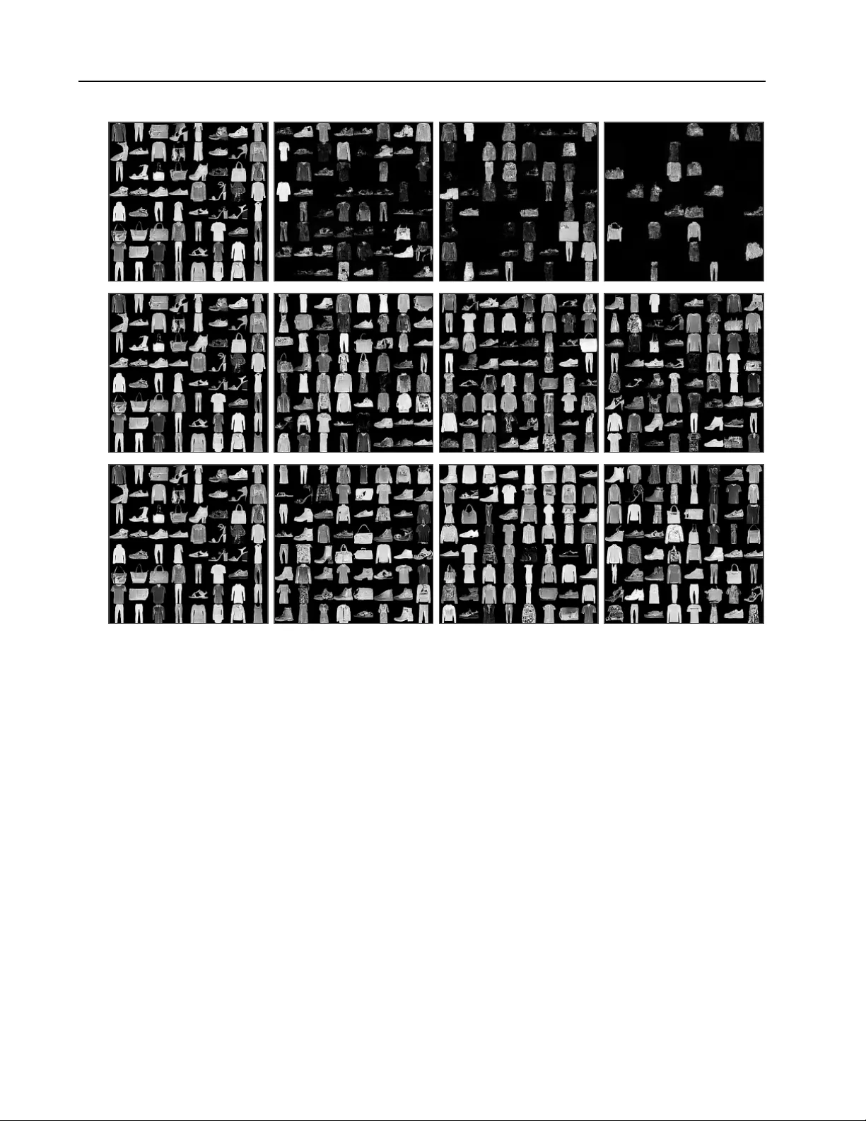
Err or Pr opagation and Model Collapse in Diffusion Models: A Theor etical Study Na ¨ ıl B. Khelifa 1 Richard E. T urner 1 Ramji V enkataramanan 1 Abstract Machine learning models are increasingly trained or ﬁne-tuned on synthetic data. Recursiv ely training on such data has been observed to signiﬁcantly degrade performance in a wide range of tasks, often characterized by a progressiv e drift aw ay from the target distrib ution. In this work, we theoretically analyze this phenomenon in the setting of score-based diffusion models. For a realistic pipeline where each training round uses a combination of synthetic data and fresh samples from the tar get distribution, we obtain upper and lower bounds on the accumulated di ver gence between the generated and target distributions. This allows us to characterize dif ferent regimes of drift, depending on the score estimation error and the proportion of fresh data used in each generation. W e also provide empirical results on synthetic data and images to illustrate the theory . 1. Introduction As generativ e AI becomes ubiquitous, synthetic data is increasingly being used for training ( Zelikman et al. , 2022 ; Gulcehre et al. , 2023 ). Howe ver , it has been observ ed that performance of a model can degrade dramatically when trained predominantly on its o wn output ( Briesch et al. , 2024 ; Alemohammad et al. , 2024a ), a phenomenon often termed model collapse ( Shumailov et al. , 2024 ; Gerstgrasser et al. , 2024a ). For example, with recursi ve self-training a generativ e model may lose the tails of the target distribution or exhibit a marked decrease in div ersity ( Dohmatob et al. , 2024b ; Shi et al. , 2025 ). In general, model collapse manifests as a progressive drift aw ay from the target distribution with each training round. In this paper , we theoretically analyze this phenomenon for score-based dif fusion models ( Sohl-Dickstein et al. , 2015 ; Ho et al. , 2020b ; Song et al. , 2021 ), which achieve state-of-the-art performance for text-to-image, text-to-audio, and video generation ( Saharia et al. , 2022 ; Liu et al. , 2023 ; Ho et al. , 2022 ) as well as in a range of scientiﬁc applications ( W atson et al. , 2023 ; Corso et al. , 2023 ). There is a growing body of theoretical work studying the effects of recursi vely training machine learning models with a combination of real and synthetic data. Howe v er , this has largely been in the context of either regression models ( Dohmatob et al. , 2024a ; 2025 ; Dey et al. , 2025 ; V u et al. , 2025 ; Garg et al. , 2025 ) or maximum-likelihood type estimators for learning parametric distributions ( Bertrand et al. , 2024 ; Suresh et al. , 2025 ; Barzilai & Shamir , 2025 ; Kanabar & Gastpar , 2025 ). V arious authors ha v e studied model collapse in diffusion and ﬂo w models empirically , and proposed techniques to mitigate it ( Alemohammad et al. , 2024b ; Shi et al. , 2025 ; Y oon et al. , 2024 ; Chen et al. , 2025 ), but to our kno wledge, there is still no theoretical analysis quantifying how the performance of dif fusion models ev olves with successi ve retraining. Setting W e study a recursiv e training procedure in which the training data in each round is a combination of fresh samples from the true data distribution and synthetic samples generated by the current diffusion model. Let p data denote the (unkno wn) true data distribution on R d . W e refer to each training round as a generation, and denote the model distribution at the end of generation i by ˆ p i for i ≥ 0 , with ˆ p 0 = p data . At each generation i ≥ 1 , the training data consists of: • a proportion α of fresh samples drawn from p data , and • a proportion (1 − α ) of synthetic samples dra wn from the current model ˆ p i . W e emphasize that the samples are not labeled as fresh or synthetic. This captures a realistic setting where the training is agnostic to how the samples were generated. Therefore, at the population lev el, the effecti v e training distribution for 1 Department of Engineering, Uni versity of Cambridge, Cambridge, United Kingdom. Correspondence to: Na ¨ ıl B. Khelifa < nbk24@cam.ac.uk > , Richard E. T urner < ret26@cam.ac.uk > , Ramji V enkataramanan < rv285@cam.ac.uk > . Pr eprint. F ebruary 19, 2026. 1 Error Pr opagation and Model Collapse in Diffusion Models F igure 1. Samples generated by a recursi vely trained model, projected onto the ﬁrst two principal components, with p data a 10 dimensional Gaussian mixture. Columns correspond to fresh data fractions α ∈ { 0 . 1 , 0 . 5 , 0 . 9 } (left to right); rows show generations 0 (start), 10 (middle), and 20 (end). At α = 0 . 1 (left column), the distrib ution progressi vely disperses as errors accumulate without suf ﬁcient fresh data. At α = 0 . 5 (center), moderate degradation occurs with visible spreading but preserv ed structure. At α = 0 . 9 (right column), the distribution remains stable throughout, demonstrating that high fresh data fractions ef fectively pre vent collapse. Experiment details in Appendix G.1 . generation i ≥ 1 is the mixture q i := α p data + (1 − α ) ˆ p i . (1) A score network is trained on samples from q i , which is then used to produce the next synthetic distribution ˆ p i +1 . This deﬁnes the recursion ˆ p i mix with p data − − − − − − − − → q i train model − − − − − − → ˆ p i +1 . (2) The goal of this work is to answer the follo wing question: In this r ecursive setting, how do err ors accumulate over generations and how does the diverg ence between ˆ p i and p data evolve? Figure 1 illustrates the effect of different mixing proportions on a recursively trained diffusion model, for p data a 10- dimensional mixture of Gaussians. Figure 8 in Appendix G.2 shows similar beha vior for the Fashion-MNIST dataset ( Xiao et al. , 2017 ), i.e., p data is the distribution that uniformly samples images from the original dataset. Learning T arget At a high-le vel, training a dif fusion model is equiv alent to learning the score function of p data corrupted with Gaussian noise, at a range of noise lev els ( Song et al. , 2021 ; Chen et al. , 2023c ). Although the intention is to learn p data , the score network at generation i is trained on samples drawn from the mixture q i . At the population lev el, the identiﬁable target of training is therefore the score of q i , not the score of p data . This mismatch between the intended target and the learned target is a fundamental source of error under recursiv e training. Furthermore, the score network does not error learn the score of q i perfectly (due to ﬁnite-sample and function approximation errors). This score matching error propagates through the stochastic differential equation (SDE) deﬁning the diffusion model (the “reverse SDE” in ( 8 ) ), because of 2 Error Pr opagation and Model Collapse in Diffusion Models which the learned distribution ˆ p i +1 will differ from q i . Characterizing this error propagation is crucial for understanding the div ergence of ˆ p i +1 from p data as i grows. W e track the ev olution of the recursion using two quantities based on the χ 2 -div ergence (deﬁned in ( 5 )): • Accumulated diver gence , measuring the di v ergence between the i -th generation model and the true data distrib ution: D i := χ 2 ( ˆ p i ∥ p data ) . (3) • The intra-gener ation diver gence, measuring the error introduced in one training round: I i := χ 2 ( ˆ p i +1 ∥ q i ) . (4) W e work primarily with the χ 2 -div er gence because, in the perturbativ e regime relev ant for our analysis, it is equiv alent to the KL div ergence up to universal constants (see empirical evidence in Figure 4 , where our bounds holds for both div er gences), while yielding a particularly con venient algebra under the refresh step q i = αp data + (1 − α ) ˆ p i that makes the cross-generation recursion explicit. Main contributions The recursion induced by training on real-synthetic mixtures in volves two competing ef fects: error mitigation from the fresh data used in each step, and error accumulation from imperfect score learning and sampling. Our contributions quantify both terms and their interaction across a gro wing number of generations. 1. Lower bound for intra-g eneration diver gence : W e provide a lo wer bound (Proposition 3.3 ) for I i that, for small score errors, is the product of two diffusion-speciﬁc terms: (i) observability of errors at the endpoint of the dif fusion path (captured by a coefﬁcient η i ), and (ii) the energy of the path-wise score error . χ 2 ( ˆ p i +1 ∥ q i ) | {z } Intra-Generational Div ergence ≳ η i |{z} Observability of Errors · ε 2 ⋆,i |{z} Score Error Energy T o our knowledge, this is the ﬁrst lower bound for diffusion models quantifying the discrepancy between the learned distribution and the tar get. 2. Intra-gener ation Diver gence Contr ol via Scor e Err or: Combining the above lo wer bound with a standard upper bound (Proposition 3.1 ), and proving an equiv alence between the score error energies on the ideal-path and the learned-path (for small errors), we sho w in Theorem 3.4 that in this re gime I i is equi v alent to the score error energy (up to constants): χ 2 ( ˆ p i +1 ∥ q i ) ≍ ε 2 ⋆,i . 3. Long-horizon re gimes and a discounted accumulation law . W e analyze the accumulated diver gence D N for small per-generation score errors, and identify a dichotomy as the generation N grows (Proposition 4.1 and Theorem 4.2 ): (i) if the score error ener gies do not decay f ast enough (e.g. a nonzero error ﬂoor so that P k ε 2 ⋆,k = + ∞ ), then D N cannot vanish with growing N ; (ii) if P k ε 2 ⋆,k < ∞ , then D N remains stable (uniformly bounded) with growing N . Moreov er , the accumulated div ergence after a ﬁnite number of generations N admits an interpretable geometrically-discounted decomposition up to a bias term: χ 2 ( ˆ p N +1 ∥ p data ) + C bias ≍ N X k =0 (1 − α ) 2( N − k ) | {z } Forgetting (real data) · ε 2 ⋆,k |{z} Accumulation (synthetic data) , which shows that errors from m generations in the past are suppressed by a factor (1 − α ) 2 m , quantifying the effect of α , the proportion of fresh data used in each training round. Qualitatively , this is consistent with empirical and theoretical work in a v ariety of settings sho wing that incorporating fresh data in each training round can mitigate model collapse, e.g. ( Gerstgrasser et al. , 2024b ; Zhu et al. , 2025 ; Bertrand et al. , 2024 ; Dey et al. , 2025 ). W e also provide experiments on simulated data and images to illustrate the v alidity of our bounds. Our results are relevant in the regime where the energy of the path-wise score error (deﬁned in ( 10 ) ) is small for all but a few generations. This regime is of interest since we seek to quantify how the intra-generation and accumulated di ver gences e volv e when the score is estimated with high accuracy in each generation. Howe ver , we note that the number of samples for the score error to be accurately estimate may grow e xponentially in the dimension d (see ( 12 )). 3 Error Pr opagation and Model Collapse in Diffusion Models Notation Bold symbols (e.g. X t , Y t ) denote R d -valued random v ariables or processes, and calligraphic symbols denote measurable sets. The space of continuous functions from [0 , T ] to R d is denoted by C ([0 , T ] , R d ) . For a stochastic process ( Z t ) t ∈ [0 ,T ] deﬁned on C ([0 , T ] , R d ) , we write La w(( Z t ) t ) for its law on path space and La w( Z t ) for the law of its marginal at time t . For two smooth probability densities p, q on R d and a con v ex function f with f (1) = 0 , the associated f -diver gence is deﬁned as D f ( p ∥ q ) = Z R d f  p ( x ) q ( x )  q ( x ) d x . (5) In particular , f ( u ) = u log u yields the K ullback–Leibler di ver gence and f ( u ) = ( u − 1) 2 yields the χ 2 -div er gence. For two nonne gati ve functions (or sequences) f and g , we write f ( x ) ≍ g ( x ) if there exist constants 0 < c 1 ≤ c 2 < ∞ such that c 1 g ( x ) ≤ f ( x ) ≤ c 2 g ( x ) . 2. Background and Model Assumptions Forward diffusion T o deﬁne the score-matching objective and the subsequent sampling procedure, we associate to each q i a forward diffusion process on a truncated time interval [ t 0 , T ] , with 0 < t 0 < T . W e consider the following variance-preserving Ornstein-Uhlenbeck process ( Karatzas & Shre ve , 2014 ; Song et al. , 2021 ): d X i t = − 1 2 X i t d t + d B t , (6) where ( B t ) t ∈ [0 ,T ] is a standard d -dimensional Brownian motion. The process is initialized with X i 0 drawn from a suitable distribution q i, 0 . Denote by q i,t := Law( X i t ) the time- t marginal of the forward process, with population score s ⋆ i ( x , t ) := ∇ x log q i,t ( x ) . Reverse-time generation and learning Under standard regularity conditions ( Anderson , 1982 ; Haussmann & P ardoux , 1986 ), the time rev ersal of ( 6 ) solves the rev erse-time SDE: d Y i,⋆ s =  − 1 2 Y i,⋆ s − s ⋆ i ( Y i,⋆ s , s )  d s + d ¯ B s , (7) integrated backward from s = T to s = 0 . Here ( ¯ B s ) s ∈ [0 ,T ] is another Brownian motion on the same probability space. If we run the reverse SDE starting from Y i,⋆ T ∼ q i,T , then Y i,⋆ 0 ∼ q i, 0 . In practice, the score s ⋆ i is unknown and is approximated by a learned network s θ i trained on samples from q i in ( 1 ) . Moreover , since the score function is often ill-behav ed and challenging to estimate as t → 0 ( Song & Ermon , 2020 ; Kim et al. , 2022 ), as done in practice we truncate the learned process at s = t 0 > 0 . W e choose q i, 0 such that q i,t 0 = q i . Plugging the learned score s θ i into the rev erse dynamics yields the learned rev erse process: d ˆ Y i s =  − 1 2 ˆ Y i s − s θ i ( ˆ Y i s , s )  d s + d ¯ B s , (8) with initialization ˆ Y i T ∼ N (0 , I d ) . The next generation model is thus denoted ˆ p i +1 := Law( ˆ Y i t 0 ) . Finally , denote the corresponding path laws on the path-space C ([ t 0 , T ] , R d ) by P ⋆ i := La w  ( Y i,⋆ s ) s ∈ [ t 0 ,T ]  , ˆ P i := La w  ( ˆ Y i s ) s ∈ [ t 0 ,T ]  , so that the time- t 0 marginals of the ideal and the learned re verse processes satisfy Y i,⋆ t 0 ∼ q i under P ⋆ i , and ˆ Y i t 0 ∼ ˆ p i +1 under ˆ P i . (9) W ith some abuse of notation, we use q i , ˆ p i +1 to both the laws and the densities with respect to the Lebesgue measure. Score err or and energies W e deﬁne the pointwise score error e i ( x , t ) := s θ i ( x , t ) − s ⋆ i ( x , t ) , and its path-wise energies ε 2 ⋆,i := E P ⋆ i " Z T t 0 ∥ e i ( Y i,⋆ s , s ) ∥ 2 2 d s # , (10) ˆ ε 2 i := E ˆ P i " Z T t 0 ∥ e i ( ˆ Y i s , s ) ∥ 2 2 d s # . (11) 4 Error Pr opagation and Model Collapse in Diffusion Models These quantities control the intra-generation di ver gence I i deﬁned in ( 4 ) . W e note that ( 10 ) is the score-matching loss for generation i ( Hyv ¨ arinen , 2005 ; V incent , 2011 ; Song & Ermon , 2019 ; Ho et al. , 2020a ). At a ﬁnite sample lev el, for a training sample D i i . i . d ∼ q i of size n i , under appropriate assumptions, the minimax-optimal score estimation error satisﬁes ( Zhang et al. , 2024 ): ε 2 ⋆,i ≲ p olylog( n i ) n − 1 i (1 /t 0 ) d/ 2 . (12) Similar bounds, relying on dif ferent assumptions, ha ve been deri ved in v arious works ( Oko et al. , 2023 ; Dou et al. , 2024 ; W ibisono et al. , 2024 ). Our results are rele vant in the regime where ε 2 ⋆,i < 1 . From ( 12 ) , this requires a training sample of size n i ∼ (1 /t 0 ) d/ 2 . Howe ver , when the distrib ution p data is supported on a lo w dimensional manifold (as is the case for images), under suitable assumptions we expect the optimal score estimation error to depend only on the intrinsic dimension d ⋆ ≪ d ( Chen et al. , 2023b ). Our main goal is to quantify how the score estimation error ( 10 ) propagates within and across generations. W e make a few simplifying assumptions to keep the analysis tractable and reduce bookkeeping. Model Assumptions The proportion α of fresh samples used for training is strictly positiv e. W e will assume p data admits a density with respect to Lebesgue measure and the model distribution ˆ p i is absolutely continuous with respect to p data , for each generation i . This is a standard assumption in analyses of dif fusion models ( Chen et al. , 2023c ; Benton et al. , 2024 ). In addition to the score estimation error , there are two other sources of error in practice. One is due to the learned re verse process ( 8 ) being initialized with Y i,⋆ T ∼ N (0 , I d ) rather than rather than Y i,⋆ T ∼ q T used for the ideal process in ( 7 ) . The KL div er gence between q T and N (0 , I d ) con verges to 0 exponentially fast in T ( Bakry et al. , 2014 ), so we ignore this error . The second source of error is the discretization error when the rev erse process is implemented in discrete-time. W e do not quantify these errors as our main goal is to obtain lower bounds on the intra-generation and accumulated errors. Obtaining error propagation bounds taking these additional sources of error into account is a direction for future work. 3. Intra-generation diver gence bounds W e now analyze the intra-g enerational mechanism by which score estimation error in generation i translates into mismatch between the sampling output ˆ p i +1 and the training distribution q i in ( 1 ) . Our goal is to relate the one-step div er gence I i deﬁned in ( 4 ) to the pathwise score-error energies deﬁned by ( 10 )-( 11 ). Key T echnical Ideas and Girsanov Quantities T o quantify how local score errors propagate to the ﬁnal samples, we use a change-of-measure ar gument based on Girsano v’ s theorem ( Girsanov , 1960 ; Le Gall , 2018 ). This is a key result in the theory of diffusion models that shows ho w the drift mismatch between the ideal and learned reverse-time processes (score error in our setting) controls the Radon-Nikodym deri vati ve of the path-space measure ˆ P i with respect to P ⋆ i . Deﬁne the error martingale M i t := − Z t t 0 e i ( Y i,⋆ s , s ) · d ¯ B s , (13) and its quadratic variation ⟨ M i ⟩ t = Z t t 0 ∥ e i ( Y i,⋆ s , s ) ∥ 2 2 d s. (14) W e also deﬁne Z i t := M i t − 1 2 ⟨ M i ⟩ t . Under mild and standard assumptions ( A1 and A2 below), Girsanov’ s theorem states that ˆ P i ≪ P ⋆ i and d ˆ P i d P ⋆ i = exp( Z i T ) . Crucially , the likelihood ratio of the terminal marginals R i := ˆ p i +1 /q i is obtained by projecting this path density onto the terminal state (Proposition B.1 ): R i ( Y i,⋆ t 0 ) := ˆ p i +1 ( Y i,⋆ t 0 ) q i ( Y i,⋆ t 0 ) = E P ⋆ i h e Z i T    Y i,⋆ t 0 i . (15) This relation is central to our analysis as it translates functional score errors (captured by Z i T ) into probabilistic drift. A key challenge in our analysis is obtain a good lo wer bound on the conditional expectation in ( 15 ). W e begin with an upper bound that follows from a standard application of Girsano v’ s theorem. 5 Error Pr opagation and Model Collapse in Diffusion Models 3.1. Upper Bound via Change of Measure Assume there exists i 0 ≥ 1 such that for all generations i ≥ i 0 , the following conditions hold. (A1) Finite drift energy along learned paths. ˆ ε 2 i := E ˆ P i " Z T t 0 ∥ e i ( ˆ Y i s , s ) ∥ 2 2 d s # < ∞ . (A2) Martingale property of the Girsanov density . The exponential e Z i T associated with the drift difference between ( 7 ) and ( 8 ) deﬁnes a true martingale on [ t 0 , T ] so that the Girsanov change of measure holds. (A more precise version in stated in Appendix B.1 .) Assumptions A1 - A2 impose no restriction on the form of the score error beyond ﬁnite quadratic energy and are standard in diffusion theory . They yield the following well-kno wn upper bound relating sampling error to the pathwise score-estimation energy ( Chen et al. , 2023a ; c ; Benton et al. , 2024 ). Proposition 3.1 (Intra-generational upper bound) . Under A1 – A2 , ˆ P i ≪ P ⋆ i and, by data pr ocessing inequality (mar ginaliza- tion to time t 0 ), KL( ˆ p i +1 ∥ q i ) ≤ KL( ˆ P i ∥ P ⋆ i ) = 1 2 ˆ ε 2 i . (16) For completeness, we gi ve the proof in Appendix B.1 . 3.2. Lower Bound V ia Error Observability The upper bound of Proposition 3.1 measures the entire path-space score error . Obtaining a div ergence lo wer bound is more challenging as we hav e to to work with the mar ginal likelihood ratio gi ven by ( 15 ). F I R S T C H A L L E N G E : O B S E RV A B I L I T Y O F E R R O R S It is possible that the path-space score error ˆ ε 2 i > 0 , but KL( ˆ p i +1 ∥ q i ) = 0 , i.e., a non-zero path-wise error may leav e no trace at the end point t 0 if it is orthogonal (in L 2 ) to all observables at t 0 . This phenomenon is intrinsic, so we need an observability condition linking path-wise perturbations to the endpoint. W e quantify the visibility of score errors at t 0 through the following coef ﬁcient. Deﬁnition 3.2 (Observability of Errors Coef ﬁcient) . Recalling the deﬁnition of M i T in ( 13 ), η i := V ar P ⋆ i  E [ M i T | Y i,⋆ t 0 ]  ε 2 ⋆,i ∈ [0 , 1] , (17) with the con vention η i := 0 if ε 2 ⋆,i = 0 . The denominator in ( 17 ) equals V ar P ⋆ i ( M i T ) , by It ˆ o isometry ( Le Gall , 2018 ). The leading term in our diver gence lower bound (Proposition 3.3 ) is proportional to η i . Hence the bound is informativ e whenev er η i > 0 . When is η i > 0 in practice? By deﬁnition, η i = 0 ⇐ ⇒ E P ⋆ i  M i T | Y i,⋆ t 0  = 0 P ⋆ i -a.s. , i.e., η i = 0 when the drift-mismatch martingale M i T is conditionally orthogonal to all terminal observ ables. This cancellation is highly non-generic: in common parametric score models (e.g. neural networks with smooth activ ations (e.g. SiLU, GeLU)), due to random initialization and stochastic optimization noise we expect η i > 0 . The experiments discussed in Appendix G suggest that in realistic data-driven setups, η i > 0 holds across generations; see Figure 7 (10-dimensional Gaussian Mixture) and Figure 9 (CIF AR-10 dataset). More generally , a simple and practically relevant suf ﬁcient condition is state dependence of the score perturbation function e i ( x , t ) : time-only (or purely path-orthogonal) perturbations can be averaged out by the conditional expectation, whereas perturbations coupled to the sample state x typically leave a detectable imprint on the endpoint. In particular , any nontrivial state-dependent afﬁne component yields observability: if e i ( x , t ) = w x + ξ ( t ) with w  = 0 and ξ independent of x , then η i > 0 . This dichotomy is illustrated empirically in Figure 2 , where state-dependent perturbations exhibit higher observ ability than time-only perturbations. 6 Error Pr opagation and Model Collapse in Diffusion Models 2 4 6 8 10 Generation i 0.00 0.05 0.10 0.15 0.20 0.25  η i (paired) 0.07 0.05 0.01 Aligned ( w i ∥ drift) Random ( w ⟂ drift) Time-only noise F igur e 2. Observability of three classes of score perturbations in CIF AR-10 ( Krizhevsky , 2009 ) diffusion sampling. W e inject controlled perturbations e i ( x , t ) and estimate the observability coefﬁcient ˆ η i = V ar( b E [ M i | Y i,⋆ t 0 ]) / V ar( M i ) using paired reverse trajectories with shared dif fusion noise. Aligned : e i ( x , t ) = w i x with w i chosen so that the error points in a direction correlated with the drift (i.e., errors push trajectories further along where they are already going). Random : e i ( x , t ) = wx with random w independent of the drift direction T ime-only : e i ( x , t ) = ξ ( t ) , independent of state. State-dependent perturbations yield higher ˆ η i , conﬁrming that errors coupled to the sample state are more visible at the terminal distribution. S E C O N D C H A L L E N G E : R A T I O O F M A R G I N A L S The ratio of mar ginals, gi ven by ( 15 ) , depends on an exponential functional of the score error along the path, projected to the endpoint. Thus, controlling marginals requires uniform integrability and moment bounds to prev ent rare trajectories from dominating e Z i T and to relate its ﬂuctuations to the scale ε 2 ⋆,i . This motiv ates the following re gularity assumptions: moment bounds on the Girsanov ratio and the quadratic v ariation in ( 14 ). (A3) L 1+ δ -integrability of the Girsanov density . There exist δ > 1 and C δ < ∞ such that the Radon–Nikodym deri v ati ve d ˆ P i d P ⋆ i = e Z i T satisﬁes sup i ≥ i 0 E P ⋆ i h e Z i T (1+ δ ) i ≤ C δ . (18) (A4) Quadratic V ariation Moment. There exists K γ < ∞ and γ > max { 2 , 4 δ − 1 } with δ > 1 deﬁned in A3 such that sup i ≥ i 0 E P ⋆ i [ ⟨ M i ⟩ 2+ γ T ] ε 2(2+ γ ) ⋆,i ≤ K γ . (19) Assumptions A3 - A4 are required to hold for generations after some i 0 > 0 , which allows to a v oid the ef fect of arbitrary or bad initializations. Moreover , since the “memory” of the bad initial steps vanishes, the long-term behavior is determined by the regime where i ≥ i 0 . Assumptions A3 - A4 are stated with free parameters to retain ﬂexibility; for concreteness, one may for instance ﬁx ( δ, γ ) = (3 , 3) . W e now state the main lo wer bound result. Proposition 3.3 (Intra-generational Lo wer Bound) . Under Assumptions A1 – A4 , the following holds for generations i ≥ i 0 . Ther e e xist constants c > 0 and C < ∞ (depending only on η i , K γ , C δ , and δ ) such that if the total scor e err or satisﬁes the perturbative condition ε 2 ⋆,i ≤ 1 , then: χ 2 ( ˆ p i +1 ∥ q i ) ≥ 1 4 · η i · ε 2 ⋆,i − C · ε 4 ⋆,i . (20) In particular , when ε 2 ⋆,i ≤ min { 1 , η i 8 C } , we obtain the clean lower bound: χ 2 ( ˆ p i +1 ∥ q i ) ≥ 1 8 · η i · ε 2 ⋆,i . 7 Error Pr opagation and Model Collapse in Diffusion Models 2 4 6 8 10 12 14 16 18 20 G e n e r a t i o n i 1 0 0 1 0 1 K L ( p i + 1 q i ) K L ( p i + 1 q i ) , = 0 . 1 1 2 2 i , = 0 . 1 K L ( p i + 1 q i ) , = 0 . 5 1 2 2 i , = 0 . 5 2 4 6 8 10 12 14 16 18 20 G e n e r a t i o n i 1 0 1 1 0 0 1 0 1 1 0 2 2 ( p i + 1 q i ) 2 ( p i + 1 q i ) , = 0 . 1 1 8 2 , i , = 0 . 1 2 ( p i + 1 q i ) , = 0 . 5 1 8 2 , i , = 0 . 5 F igure 3. Empirical veriﬁcation of intra-generational error bounds f or a Gaussian mixture. p data ∼ 1 5 P 5 k =1 N ( µ k , σ 2 I 10 ) ∈ R 10 . Left: Upper bound veriﬁcation (Proposition 3.1 ). The KL diver gence KL( ˆ p i +1 ∥ q i ) between the learned distribution and the training mixture remains bounded by 1 2 ˆ ε 2 i . The bound is tight at early generations and becomes conservati ve as the system equilibrates. Right: Lower bound veriﬁcation (Proposition 3.3 ). The χ 2 div er gence I i = χ 2 ( ˆ p i +1 ∥ q i ) is bounded belo w by 1 8 ˆ η i ε 2 ⋆,i , where ˆ η i is the estimated observability coefﬁcient. Shaded regions indicate ± 1 standard de viation across runs. Both bounds hold consistently across α ∈ { 0 . 1 , 0 . 5 } , validating the theoretical frame work. Experiment details are given in Appendix G.1 . The proof is given in Appendix D . The upper bounds of Propositions 3.1 and 3.3 are illustrated in Figure 3 for a 10 - dimensional Gaussian mixture, and compared with the empirically computed div ergences. 3.3. T wo-sided equivalence Proposition 3.1 controls the intra-generation div ergence from abov e in terms of the learned-path energy ˆ ε 2 i , whereas Proposition 3.3 provides a matching lower bound in terms of the ideal-path energy ε 2 ⋆,i , up to the observability factor η i and higher-order terms. T o turn these complementary statements into a single equi v alence I i = χ 2 ( ˆ p i +1 ∥ q i ) ≍ ε 2 ⋆,i , the two energies ε 2 ⋆,i (under P ⋆ i ) and ˆ ε 2 i (under ˆ P i ) as well as the two di ver gences KL (upper bound) and χ 2 (lower bound) need to be related. Under Assumptions A3 and A4 , we sho w that these ener gies and di ver gences are equiv alent. Combining these equiv alence results with Propositions 3.1 and 3.3 yields the following two-sided control of the intra-generational div ergence. Theorem 3.4 (T wo-Sided bounds for intra-generational diver gence) . Under Assumptions A1 - A4 , the following holds for generations i ≥ i 0 . There exist constants c > 0 and C < ∞ (depending only on δ, C δ , γ , K γ ) such that, when the perturbative condition ε 2 ⋆,i ≤ min { 1 , η i 8 C } holds, we have: 1 4 η i ε 2 ⋆,i − C · ε 4 ⋆,i ≤ χ 2 ( ˆ p i +1 ∥ q i ) ≤ 4 ε 2 ⋆,i + cε 4 ⋆,i . In particular , for suf ﬁciently small ε 2 ⋆,i , we have χ 2 ( ˆ p i +1 ∥ q i ) ≍ ε 2 ⋆,i . (21) The proof is giv en in Appendix E . This theorem sho ws that the intra-generational div er gence is controlled by the pathwise score-error energy and that the tw o are equi v alent (up to constants), up to observ ability and tail ef fects. Figure 4 indicates these bounds hold in a fully data-driv en experiment for both the χ 2 and KL div ergences. 4. Error Accumulation Acr oss Generations Theorem 3.4 shows that when the score error is observable (i.e., η i > 0 ), the intra-generational diver gence satisﬁes I i = χ 2 ( ˆ p i +1 ∥ q i ) is equiv alent (up to constants) to ε 2 ⋆,i in the perturbativ e regime. W e now study how this div ergence propagates through the recursion ( 2 ) ov er many generations, recalling our assumption that the refresh rate α > 0 . A ke y observ ation is that the fresh samples introduced in each generation contracts the accumulated di vergence. Indeed, a simple calculation (Lemma F .1 ) shows that χ 2 ( ˆ p i ∥ p data ) = (1 − α ) 2 χ 2 ( ˆ p i ∥ p data ) . In contrast, the score error in 8 Error Pr opagation and Model Collapse in Diffusion Models 2 4 6 8 10 12 14 16 18 20 G e n e r a t i o n i 1 0 1 1 0 0 1 0 1 1 0 2 Divergence = 0 . 1 2 ( p i + 1 q i ) K L ( p i + 1 q i ) 4 2 , i 1 4 i 2 , i 2 4 6 8 10 12 14 16 18 20 G e n e r a t i o n i 1 0 1 1 0 0 1 0 1 Divergence = 0 . 5 2 ( p i + 1 q i ) K L ( p i + 1 q i ) 4 2 , i 1 4 i 2 , i F igur e 4. T wo-sided control of intra-generation diver gence. p data ∼ 1 5 P 5 k =1 N ( µ k , σ 2 I 10 ) ∈ R 10 . W e track the evolution of the div er gences I i = χ 2 ( ˆ p i +1 ∥ q i ) and I KL i = KL( ˆ p i +1 ∥ q i ) (solid lines with markers) across 20 generations for low ( α = 0 . 1 , left) and high ( α = 0 . 5 , right) fresh data ratios. Consistent with Theorem 3.4 , the intra-generational diver gences are ef fecti vely lo wer and upper bounded between by the pathwise score error energy (dashed upper bound = 4 ε 2 ⋆,i ) and the observability-weighted lo wer bound (dotted line = 1 4 ˆ η i ε 2 ⋆,i , where ˆ η i is the estimated observability of errors, as detailed in Appendix G.1 ). Shaded regions indicate ± 1 standard deviation across runs. the next round of training increases the accumulated di vergence. These two competing ef fects determine the e volution of D i = χ 2 ( q i ∥ p data ) as i gro ws. W e distinguish two cases, assuming small score errors in each generation: if P i ≥ 0 ε 2 ⋆,i = ∞ , then we show that D i and cannot con ver ge to 0 . On the other hand, if P i ≥ 0 ε 2 ⋆,i < ∞ , we show that (up to constants) D i is giv en by a discounted sum of score error energies from past generations. 4.1. Persistent Err ors Proposition 4.1 (Persistent Errors) . Assume A1 - A4 , and that for i ≥ i 0 , η i ≥ η > 0 and ε 2 ⋆,i ≤ min { 1 , η i 8 C } . Then: (i) Non-summable score error implies non-summable global drift. If P i ≥ 0 ε 2 ⋆,i = + ∞ , then P i ≥ 0 D i = + ∞ and ( D i ) i ≥ 0 cannot con verge to 0 . (ii) A score-error ﬂoor implies persistent accumulated div ergence. If ε 2 ⋆,i ≥ ε > 0 for all sufﬁciently lar ge i , then lim sup i →∞ D i ≥ α 16(1 + (1 − α ) 2 ) · η ε, In particular , the sequence ( D i ) exhibits inﬁnitely many macr oscopic deviations fr om p data . 4.2. Controlled Err ors W e now bound the accumulated div ergence D i when the score errors ε 2 ⋆,i are summable, under a technical assumption deﬁned in terms of an adaptiv e tail set. An adaptive tail assumption For a constant ζ i ∈ (0 , 1) , deﬁne the adapti ve “good” set G i := { x :   ˆ p i ( x ) /p data ( x ) − 1   ≤ p D i /ζ i } . (22) Since E p data [ | ˆ p i ( x ) /p data − 1 | 2 ] = D i , Chebyshev’ s inequality implies p data ( G c i ) ≤ ζ i . As D i grows, the set G i expands and G c i consists of the regions where where ˆ p i /p data is increasingly atypical. W e then assume that the training distribution q i does not ov er-emphasize this tail re gion in the follo wing sense. (A5) There exist a generation i 0 ≥ 0 such that, for the δ in Assumption A3 and p ′ := δ +1 δ − 1 , there exists a constant C ζ > 0 such that, sup i ≥ i 0 n ζ − 1 i E q i   q i p data  p ′ 1 G c i  o ≤ C ζ . 9 Error Pr opagation and Model Collapse in Diffusion Models 0 3 6 9 12 15 18 S o u r c e G e n e r a t i o n i 0 3 6 9 12 15 18 C u r r e n t G e n e r a t i o n N 0 3 6 9 12 15 18 S o u r c e G e n e r a t i o n i 0 3 6 9 12 15 18 0 3 6 9 12 15 18 S o u r c e G e n e r a t i o n i 0 3 6 9 12 15 18 0.0 0.2 0.4 0.6 0.8 1.0 Fractional Contribution M e m o r y S t r u c t u r e : H o w P a s t E r r o r s C o n t r i b u t e t o D N F igure 5. Geometrically-discounted decomposition of accumulated diver gence in ( 23 ) , for p data = 1 5 P 5 k =1 N ( µ k , σ 2 I 10 ) ∈ R 10 . Each panel shows contrib utions of ε 2 ⋆,i to the current global di ver gence D N = χ 2 ( ˆ p N ∥ p data ) , for i ≤ N . Left ( α = 0 . 1 ): Errors persist across many generations, creating a wide band of contrib utions. Center ( α = 0 . 5 ): Intermediate regime with moderate memory decay . Right ( α = 0 . 9 ): Short memory—only the most recent generation dominates, yielding a sharp diagonal structure. The plots are consistent with Theorem 4.2 , conﬁrming that higher fractions of fresh data accelerate the for getting of past errors. Experiment details in Appendix G.1 . From the deﬁnition of q i in ( 1 ) , we know that q i /p data = α + (1 − α ) ˆ p i /p data , which can blow up on G c i only if ˆ p i /p data is large there. Therefore, ( A5 ) is a local condition on a v anishing tail set, which rules out spurious hea vy tails that may cause the synthetic model to place large mass in re gions where where p data is tiny . Theorem 4.2 (Discounted accumulation of errors) . Assume A1 - A5 , and that i ≥ i 0 , we have η i ≥ η > 0 and ε 2 ⋆,i ≤ min n 1 , η i 8 C o . Also assume that ∞ X i =0 ε 2 ⋆,i < ∞ . Then, ther e e xists a constant C bias deﬁned in Equation ( 112 ) such that for eac h gener ation N ≥ i 0 , D N +1 + C bias ≍ N X i = i 0 (1 − α ) 2( N − i ) ε 2 ⋆,i + (1 − α ) 2( N +1 − i 0 ) D i 0 . (23) The proof is giv en in Appendix F .3 , where we deriv e upper and lo wer bounds for D N +1 with e xplicit constants. Theorem 4.2 shows that in the regime where the score errors are small and summable, the accummulated di vergence is a geometrically- discounted sum of square errors. In particular, errors from m generations in the past are suppressed by a factor (1 − α ) 2 m , and the larger the proportion of fresh training samples in each round, the higher the rate of “forgetting” score errors. Qualitativ ely , this is consistent with the ﬁndings in many dif ferent settings that incorporating fresh data in each training round can mitigate model collapse ( Gerstgrasser et al. , 2024b ; Zhu et al. , 2025 ; Bertrand et al. , 2024 ; Dey et al. , 2025 ). Figure 5 illustrates the decomposition of Theorem 4.2 for a 10 -dimensional Gaussian mixture, tracking the contribution to D N +1 of each term in the sum in ( 23 ) . Figure 10 in Appendix G.3 shows the same behavior on the Fashion-MNIST dataset ( Xiao et al. , 2017 )). Figure 6 in Appendix G.1 illustrates that the functional dependence predicted by Theorem 4.2 accurately captures the observed gro wth across generations in the 10-dimensional Gaussian mixture setting. 5. Conclusion and Future W ork W e analyzed recursiv e training of dif fusion models with a ﬁxed proportion α > 0 of fresh data in each training round. W e deriv ed lower and upper bounds on the intra-generation and accumulated diver gences, in terms of the path-wise energy of the score error in each generation. An essential component of our lo wer bound is the observ ability coef ﬁcient in ( 17 ) , which quantiﬁes the fraction of the path-wise error ener gy that manifests in the learned distrib ution. The paper focuses on the setting where the score error ener gy in each generation is small. An important direction for future work is to establish bounds in the large error re gime. Obtaining a lo wer bound in this re gime, e v en for one generation, is challenging because the ratio between the learned and ideal densities (gi ven by the projection of the path-wise ratio in ( 15 ) ) cannot be linearized with 10 Error Pr opagation and Model Collapse in Diffusion Models reasonable control of the remainder term. Another direction for further work is to taking into account the discretization error due to the diffusion being implemented in discrete-time. Finally , a key open question is: is there is a limiting distribution to which the model con verges when recursi vely trained, and if so, ho w does it depend on α and p data ? References Alemohammad, S., Casco-Rodriguez, J., Luzi, L., Humayun, A. I., Babaei, H., LeJeune, D., Siahkoohi, A., and Baraniuk, R. Self-consuming generative models go MAD. In The T welfth International Confer ence on Learning Repr esentations , 2024a. Alemohammad, S., Humayun, A. I., Agarwal, S., Collomosse, J., and Baraniuk, R. Self-improving dif fusion models with synthetic data. arXiv pr eprint arXiv:2408.16333 , 2024b. Anderson, B. D. Rev erse-time diffusion equation models. Stochastic Pr ocesses and their Applications , 12(3):313–326, 1982. Bakry , D., Gentil, I., and Ledoux, M. Analysis and Geometry of Markov Diffusion Oper ators , v olume 348 of Grundlehr en der mathematischen W issenschaften . Springer , 2014. Barzilai, D. and Shamir , O. When models don’t collapse: On the consistency of iterativ e MLE, 2025. Bene ˇ s, V . E. Existence of optimal stochastic control laws. SIAM Journal on Contr ol , 9(3):446–472, 1971. Benton, J., Bortoli, V . D., Doucet, A., and Deligiannidis, G. Nearly d -linear con vergence bounds for dif fusion models via stochastic localization. In The T welfth International Conference on Learning Repr esentations , 2024. Bertrand, Q., Bose, A. J., Duplessis, A., Jiralerspong, M., and Gidel, G. On the stability of iterativ e retraining of generativ e models on their own data. In International Confer ence on Learning Repr esentations , 2024. Briesch, M., Sobania, D., and Rothlauf, F . Large language models suffer from their own output: An analysis of the self-consuming training loop, 2024. Burkholder , D. L., Davis, B. J., and Gundy , R. F . Inte gral inequalities for con ve x functions of operators on martingales. In Pr oceedings of the Sixth Berkele y Symposium on Mathematical Statistics and Pr obability , volume II, pp. 223–240, Berkeley and Los Angeles, 1972. Uni versity of California Press. Cameron, R. H. and Martin, W . T . Transformations of weiner integrals under translations. Annals of Mathematics , 45(2): 386–396, 1944. Chen, H., Lee, H., and Lu, J. Improved analysis of score-based generati v e modeling: User-friendly bounds under minimal smoothness assumptions. International Confer ence on Machine Learning , pp. 4735–4763, 2023a. Chen, M., Huang, K., Zhao, T ., and W ang, M. Score approximation, estimation and distribution recov ery of diffusion models on low-dimensional data. In Pr oceedings of the 40th International Conference on Mac hine Learning , 2023b. Chen, S., Che wi, S., Li, J., Li, Y ., Salim, A., and Zhang, A. R. Sampling is as easy as learning the score: theory for diffusion models with minimal data assumptions. International Confer ence on Learning Repr esentations , 2023c. Chen, Z., Zhang, T ., and Y ang, Y . Analyzing and mitigating model collapse in rectiﬁed ﬂow models. arXiv preprint arXiv:2502.05422 , 2025. Corso, G., St ¨ ark, H., Jing, B., Barzilay , R., and Jaakkola, T . S. Diffdock: Diffusion steps, twists, and turns for molecular docking. In The Eleventh International Confer ence on Learning Representations , 2023. Dey , A., Gerstgrasser, M., and Donoho, D. L. Univ ersality of the π 2 / 6 pathway in av oiding model collapse. arXiv pr eprint arXiv:2504.01656 , 2025. Dohmatob, E., Feng, Y ., and Kempe, J. Model collapse demystiﬁed: The case of regression. arXiv preprint , 2024a. 11 Error Pr opagation and Model Collapse in Diffusion Models Dohmatob, E., Feng, Y ., Y ang, P ., Charton, F ., and K empe, J. A tale of tails: Model collapse as a change of scaling la ws. arXiv pr eprint arXiv:2402.07043 , 2024b. Dohmatob, E., Feng, Y ., Subramonian, A., and Kempe, J. Strong model collapse. In International Confer ence on Learning Repr esentations , 2025. Dol ´ eans-Dade, C. Quelques applications de la formule de changement de variables pour les semimartingales. Zeitschrift f ¨ ur W ahrscheinlic hkeitstheorie und V erwandte Gebiete , 16(3):181–194, 1970. Dou, Z., Kotekal, S., Xu, Z., and Zhou, H. H. From optimal score matching to optimal sampling, 2024. arXiv preprint Garg, A., Bhattacharya, S., and Sur , P . Preventing model collapse under o verparametrization: Optimal mixing ratios for interpolation learning and ridge regression. arXiv preprint , 2025. Gerstgrasser , M., Schaeffer , R., Dey , A., Rafailov , R., Sleight, H., Hughes, J., Korbak, T ., Agrawal, R., P ai, D., Gromov , A., Roberts, D. A., Y ang, D., Donoho, D. L., and Ko yejo, S. Is model collapse ine vitable? Breaking the curse of recursion by accumulating real and synthetic data. arXiv pr eprint arXiv:2404.01413 , 2024a. Gerstgrasser , M., Schaeffer , R., Dey , A., Rafailov , R., Sleight, H., Hughes, J., Korbak, T ., Agrawal, R., P ai, D., Gromov , A., Roberts, D. A., Y ang, D., Donoho, D. L., and K oyejo, S. Is model collapse inevitable? breaking the curse of recursion by accumulating real and synthetic data. In ICML W orkshop on F oundation Models in the W ild , 2024b. Girsanov , I. V . On transforming a certain class of stochastic processes by absolutely continuous substitution of measures. Theory of Pr obability & Its Applications , 5(3):285–301, 1960. Gulcehre, C., Paine, T . L., Sriniv asan, S., K onyushk ov a, K., W eerts, L., Sharma, A., Siddhant, A., Ahern, A., W ang, M., Gu, C., Macherey , W ., Doucet, A., Firat, O., and de Freitas, N. Reinforced self-training (rest) for language modeling, 2023. Haussmann, U. G. and Pardoux, E. Time re versal of diffusions. The Annals of Pr obability , pp. 1188–1205, 1986. Ho, J., Jain, A., and Abbeel, P . Denoising dif fusion probabilistic models. In Proceedings of the 34th International Conference on Neural Information Pr ocessing Systems , 2020a. Ho, J., Jain, A., and Abbeel, P . Denoising dif fusion probabilistic models. In Advances in Neural Information Pr ocessing Systems , volume 33, pp. 6840–6851, 2020b. Ho, J., Salimans, T ., Gritsenko, A., Chan, W ., Norouzi, M., and Fleet, D. J. V ideo diffusion models. Advances in neural information pr ocessing systems , 35:8633–8646, 2022. Hyv ¨ arinen, A. Estimation of non-normalized statistical models by score matching. Journal of Machine Learning Resear c h , 6:695–709, 2005. Kanabar , M. and Gastpar , M. Model non-collapse: Minimax bounds for recursi ve discrete distribution estimation. IEEE T ransactions on Information Theory , 2025. doi: 10.1109/TIT .2025.3649611. Karatzas, I. and Shrev e, S. Br ownian motion and stochastic calculus . Springer , 2014. Kim, D., Shin, S., Song, K., Kang, W ., and Moon, I.-C. Soft truncation: A univ ersal training technique of score-based dif fusion model for high precision score estimation. In International Confer ence on Machine Learning , pp. 11201–11228, 2022. Krizhevsk y , A. Learning multiple layers of features from tiny images. T echnical Report 0, Univ ersity of T oronto, 2009. URL https://www.cs.toronto.edu/ ˜ kriz/cifar.html . Le Gall, J.-F . Brownian Motion, Martingales, and Stoc hastic Calculus . Springer Publishing Company , Incorporated, 2018. Liu, H., Chen, Z., Y uan, Y ., Mei, X., Liu, X., Mandic, D., W ang, W ., and Plumbley , M. D. Audioldm: T ext-to-audio generation with latent diffusion models. In International Confer ence on Machine Learning , pp. 21450–21474, 2023. 12 Error Pr opagation and Model Collapse in Diffusion Models Noviko v , A. A. On an identity for stochastic integrals. Theory of Pr obability & Its Applications , 17(4):717–720, 1973. Oko, K., Akiyama, S., and Suzuki, T . Diffusion models are minimax optimal distribution estimators. International Confer ence on Mac hine Learning , 2023. Revuz, D. and Y or, M. Continuous martingales and Br ownian motion . Grundlehren der mathematischen W issenschaften. Springer , 3. ed edition, 1999. Saharia, C., Chan, W ., Saxena, S., Lit, L., Whang, J., Denton, E., Ghasemipour , S. K. S., A yan, B. K., Mahdavi, S. S., Gontijo-Lopes, R., Salimans, T ., Ho, J., Fleet, D. J., and Norouzi, M. Photorealistic text-to-image diffusion models with deep language understanding. In Pr oceedings of the 36th International Confer ence on Neur al Information Pr ocessing Systems , 2022. Shi, L., W u, M., Zhang, H., Zhang, Z., T ao, M., and Qu, Q. A closer look at model collapse: From a generalization-to- memorization perspectiv e, 2025. arXiv preprint arXi v:2509.16499. Shumailov , I., Shumaylov , Z., Zhao, Y ., Papernot, N., Anderson, R., and Gal, Y . AI models collapse when trained on recursiv ely generated data. Natur e , 631(8022):755–759, 2024. Silverman, B. W . Density Estimation for Statistics and Data Analysis . Chapman and Hall, 1986. Sohl-Dickstein, J., W eiss, E., Maheswaranathan, N., and Ganguli, S. Deep unsupervised learning using nonequilibrium thermodynamics. In Pr oceedings of the 32nd International Conference on Mac hine Learning , 2015. Song, Y . and Ermon, S. Generati ve modeling by estimating gradients of the data distribution. Advances in Neural Information Pr ocessing Systems , 32, 2019. Song, Y . and Ermon, S. Improv ed techniques for training score-based generati ve models. Advances in Neural Information Pr ocessing Systems , 33:12438–12448, 2020. Song, Y ., Sohl-Dickstein, J., Kingma, D. P ., Kumar , A., Ermon, S., and Poole, B. Score-based generativ e modeling through stochastic differential equations. In International Confer ence on Learning Repr esentations , 2021. Suresh, A. T ., Thangaraj, A., and Khandav ally , A. N. K. Rate of model collapse in recursive training. In International Confer ence on Artiﬁcial Intelligence and Statistics , pp. 1396–1404, 2025. V incent, P . A connection between score matching and denoising autoencoders. Neural Computation , 23(7):1661–1674, 2011. V u, H. A., Ree ves, G., and W enger , E. What happens when generative AI models train recursi vely on each others’ outputs?, 2025. W atson, J. L., Juergens, D., Bennett, N. R., T rippe, B. L., Y im, J., Eisenach, H. E., Ahern, W ., Borst, A. J., Ragotte, R. J., Milles, L. F ., et al. De nov o design of protein structure and function with rfdiffusion. Natur e , 620(7976):1089–1100, 2023. W ibisono, A., W u, Y ., and Y ang, K. Y . Optimal score estimation via empirical Bayes smoothing. In The Thirty Seventh Annual Confer ence on Learning Theory , pp. 4958–4991, 2024. Xiao, H., Rasul, K., and V ollgraf, R. Fashion-MNIST: a no vel image dataset for benchmarking machine learning algorithms, 2017. Y oon, Y ., Hu, D., W eissbur g, I., Qin, Y ., and Jeong, H. Model collapse in the self-consuming chain of diffusion ﬁnetuning: A nov el perspecti ve from quantitati ve trait modeling. In ICLR W orkshop on Navigating and Addressing Data Pr oblems for F oundation Models , 2024. Zelikman, E., W u, Y ., Mu, J., and Goodman, N. Star: Bootstrapping reasoning with reasoning. Advances in Neural Information Pr ocessing Systems , 35:15476–15488, 2022. Zhang, K., Y in, C. H., Liang, F ., and Liu, J. Minimax optimality of score-based diffusion models: beyond the density lo wer bound assumptions. In Pr oceedings of the 41st International Conference on Mac hine Learning , 2024. Zhu, H., W ang, F ., Ding, T ., Qu, Q., and Zhu, Z. Analyzing and mitigating model collapse in rectiﬁed ﬂow models, 2025. 13 Error Pr opagation and Model Collapse in Diffusion Models A. Preliminaries and notation f or Appendices W e consider rev erse-time dif fusions on the interv al [ t 0 , T ] (integrated from T down to t 0 ). Let ¯ B = ( ¯ B s ) s ∈ [ t 0 ,T ] denote a standard Brownian motion in re verse time on a ﬁltered space (Ω , F , ( F s ) s ∈ [ t 0 ,T ] ) . Indexing. The superscript i denotes the gener ation (self-training iteration). W ithin each generation we compare: (i) an ideal rev erse process (driven by the e xact score) and (ii) a learned reverse process (dri ven by the estimated score). Reverse-time SDEs and path measur es. For s ∈ [ t 0 , T ] , the ideal and learned rev erse-time processes solve d Y i,⋆ s = h − 1 2 Y i,⋆ s − s ⋆ i ( Y i,⋆ s , s ) i d s + d ¯ B s , d ˆ Y i s = h − 1 2 ˆ Y i s − s θ i ( ˆ Y i s , s ) i d s + d ¯ B s , with independent initializations Y i,⋆ T , ˆ Y i T ∼ N (0 , I d ) . W e write P ⋆ i (resp. ˆ P i ) for the law on path space C ([ t 0 , T ] , R d ) induced by Y i,⋆ (resp. ˆ Y i ). Score err or and energy . The score (drift) discrepancy is e i ( x , t ) := s θ i ( x , t ) − s ⋆ i ( x , t ) , and we use the shorthand e i ( s ) := e i ( Y i,⋆ s , s ) or e i ( ˆ Y i s , s ) depending on the ambient measure. W e distinguish two integrated error ener gies: ε 2 ⋆,i := E P ⋆ i " Z T t 0 ∥ e i ( Y i,⋆ s , s ) ∥ 2 d s # , ˆ ε 2 i := E ˆ P i " Z T t 0 ∥ e i ( ˆ Y i s , s ) ∥ 2 2 d s # . Marginal likelihood ratios. W e denote the marginal density ratios by R i ( x ) := ˆ p i +1 ( x ) q i ( x ) , T i ( x ) := q i ( x ) p data ( x ) , where q i := αp data + (1 − α ) ˆ p i . Diver gences. W e denote, for a generation i ≥ 0 and α ∈ (0 , 1) . I i := χ 2 ( ˆ p i +1 ∥ q i ) = E q i [( R i − 1) 2 ] , D i := χ 2 ( ˆ p i ∥ p data ) . Norms. For any r > 0 and an y random v ariable X , we denote the L r ( p X ) norm with respect to the measure p X by , ∥ X ∥ r := E p X  X r  1 /r . Perturbati ve Regime. The perturbed regime is referred to as the setting where the exist a generation i 0 ≥ 0 such that, ε 2 ⋆,i ≤ min n 1 , η i 8 C o , ∀ i ≥ i 0 , where the constant C := 1+ K γ 8 + 1 4  C BDG (4 p ′ ) K 2 p ′ 2+ γ γ  1 /p ′ C 1 /p δ , is deﬁned in Proposition D.1 . B. Intra-generational likelihood ratios via Girsanov’ s theorem B.1. Proof of Upper Bound (Pr oposition 3.1 ) W e recall the deﬁnitions of the ideal and learned rev erse-time processes on s ∈ [ t 0 , T ] (integrated backward from T to t 0 ) from ( 7 ) and ( 8 ) , with independent initializations Y i,⋆ T , ˆ Y i T ∼ N (0 , I d ) . Recall we deﬁned two path-space probability measures P ⋆ i and ˆ P i on the path space C ([ t 0 , T ] , R d ) : • P ⋆ i : The law of the ideal re verse-time process Y i,⋆ . It is initialized at end time T with Gaussian noise, and its dynamics are driv en by the exact score s ⋆ i . Its terminal marginal at t 0 is the current mixing distribution q i . 14 Error Pr opagation and Model Collapse in Diffusion Models • ˆ P i : The law of the learned rev erse-time process ˆ Y i . It is initialized at T with Gaussian noise, and its dynamics are driv en by the approximate score s θ i . Its terminal marginal at t 0 is the next-generation distrib ution ˆ p i +1 . The drift discrepanc y is gi v en by the score error: e i ( x , t ) := ˆ s θ i ( x , t ) − s ⋆ i ( x , t ) . Recall that we operate under the following assumptions: A1 Finite drift energy . The learned path measure satisﬁes E ˆ P i [ R T t 0 ∥ e i ( ˆ Y s , s ) ∥ 2 2 d s ] < ∞ . A2 Martingale property . From ( 13 )-( 14 ) recall that for s ∈ [ t 0 , T ] , M i s := − Z s t 0 e i ( Y i,⋆ u , u ) · d ¯ B u , ⟨ M i ⟩ s := Z s t 0 ∥ e i ( Y i,⋆ u , u ) ∥ 2 2 d u, Z i s = M i s − 1 2 ⟨ M i ⟩ s . Deﬁne the Dol ´ eans–Dade exponential U s := exp  M i s − 1 2 ⟨ M i ⟩ s  . W e assume ( U s ) s ∈ [ t 0 ,T ] deﬁnes a true P ⋆ i -martingale on [ t 0 , T ] . Discussion on Assumptions A1 and A2 . These assumptions ensures that the Girsanov transformation yields a valid probability measure (i.e., E P ⋆ i [ U T ] = 1 ). While U s is guaranteed to be a local martingale by construction, dif ferent suf ﬁcient conditions can be found in the literature to guarantee the full martingale status. The most common ones are: • Noviko v’ s condition ( Novikov , 1973 ): E P ⋆ i " exp 1 2 Z T t 0 ∥ e i ( Y i,⋆ s , s ) ∥ 2 2 d s !# < ∞ . • Bene ˇ s Condition ( Bene ˇ s , 1971 ) : the drift discrepancy satisﬁes a linear gro wth bound ∥ e i ( x , t ) ∥ 2 ≤ C (1 + ∥ x ∥ 2 ) , C > 0 . In the context of dif fusion models parameterized by neural networks, this holds if the netw ork weights are ﬁnite and the acti v ation functions are Lipschitz (e.g., ReLU, SiLU) or bounded (e.g., T anh, Sigmoid), pro vided the domain is effecti vely bounded or the growth is controlled. • Stopping T ime Condition. Finally , another popular assumption relies on stopping times. Formally , the exponential process ( U s ) s ∈ [ t 0 ,T ] is always a local martingale . This implies the existence of a non-decreasing sequence of stopping times { τ n } n ≥ 1 such that τ n ↑ T almost surely as n → ∞ , and for every n , the stopped process ( U s ∧ τ n ) s ∈ [ t 0 ,T ] is a true martingale. A canonical choice for these stopping times is deﬁned by the accumulation of the drift energy: τ n := inf  s ∈ [ t 0 , T ] : Z s t 0 ∥ e i ( Y i,⋆ u , u ) ∥ 2 2 d u ≥ n  ∧ T . (24) By deﬁnition, the accumulated energy up to time τ n is bounded by n . Consequently , the conditional Novikov criterion is trivially satisﬁed for the stopped process: E  exp  1 2 Z τ n t 0 ∥ e i ( Y i,⋆ s , s ) ∥ 2 2 d u  ≤ e n/ 2 < ∞ . This guarantees that E [ U τ n ] = 1 for all n . Assumption A2 is therefore equiv alent to the condition that the sequence is uniformly integrable, allowing the equality to hold in the limit: E [ U T ] = lim n →∞ E [ U τ n ] = 1 . This stopping time condition has been used in pre vious analyses of the con vergence properties of diffusion models ( Chen et al. , 2023c ; Benton et al. , 2024 ). 15 Error Pr opagation and Model Collapse in Diffusion Models Pr oof of Proposition 3.1 . Step 1: Pathwise Change of Measur e via Girsano v . The ideal process Y i,⋆ and learned process ˆ Y i are deﬁned on the ﬁltered probability space (Ω , F , ( F s ) s ∈ [ t 0 ,T ] , P ⋆ i ) equipped with the standard Bro wnian motion ¯ B . They share the same diffusion coefﬁcient (the identity matrix) and differ only in their drift terms. Speciﬁcally , the drift difference is ∆ b ( x , s ) = − e i ( x , s ) . T o relate their laws, we employ Girsanov’ s theorem ( Cameron & Martin , 1944 ; Girsanov , 1960 ; Le Gall , 2018 ). The candidate density process is the stochastic exponential (Dol ´ eans-Dade exponential ( Dol ´ eans-Dade , 1970 )) of M i , U s = exp  M i s − 1 2 ⟨ M i ⟩ s  . By It ˆ o’ s formula ( Karatzas & Shrev e , 2014 ; Le Gall , 2018 ), U s is a nonnegati ve local martingale under P ⋆ i and hence a supermartingale. By Assumption A2 , ( U s ) s ∈ [ t 0 ,T ] is in fact a (uniformly integrable) martingale, so in particular E P ⋆ i [ U T ] = U t 0 = 1 . Therefore, we can deﬁne the probability measure ˆ P i by the Radon-Nikodym deri v ati ve: d ˆ P i d P ⋆ i (( Y ⋆,i s ) s ∈ [ t 0 ,T ] ) = U T = exp − Z T t 0 e i ( Y ⋆,i s , s ) · d ¯ B s − 1 2 Z T t 0 ∥ e i ( Y ⋆,i s , s ) ∥ 2 2 d s ! . Under this new measure ˆ P i , the process ˆ B s := ¯ B s + R s t 0 e i ( Y u , u )d u is a standard Brownian motion (by the Girsanov theorem), and the coordinate process Y satisﬁes the SDE of the learned dif fusion ˆ Y i . Thus, ˆ P i is precisely the law of the learned process. Step 2: KL Diver gence Calculation. The Kullback-Leibler diver gence is deﬁned as KL( ˆ P i ∥ P ⋆ i ) = E ˆ P i [log d ˆ P i d P ⋆ i ] . W e express the log-density ratio in terms of the process ˆ Y (gov erned by ˆ P i ). Under ˆ P i , we can write d ¯ B s = d ˆ B s − e i ( ˆ Y s , s )d s , where ˆ B is a standard Brownian motion under ˆ P i . Substituting this into the log-likelihood ratio: log d ˆ P i d P ⋆ i (( ˆ Y s ) s ∈ [ t 0 ,T ] ) = − Z T t 0 e i ( ˆ Y s , s ) · d ¯ B s − 1 2 Z T t 0 ∥ e i ( ˆ Y s , s ) ∥ 2 2 d s = − Z T t 0 e i · (d ˆ B s − e i d s ) − 1 2 Z T t 0 ∥ e i ( ˆ Y s , s ) ∥ 2 2 d s = − Z T t 0 e i ( ˆ Y s , s ) · d ˆ B s + 1 2 Z T t 0 ∥ e i ( ˆ Y s , s ) ∥ 2 2 d s. T aking expectation under ˆ P i : E ˆ P i " log d ˆ P i d P ⋆ i # = E ˆ P i " − Z T t 0 e i · d ˆ B s # + 1 2 E ˆ P i " Z T t 0 ∥ e i ( ˆ Y s , s ) ∥ 2 2 d s # . The ﬁrst term is the e xpectation of a stochastic inte gral. Under Assumption A1 , the integrand is square-inte grable, so the stochastic integral is a true martingale starting at 0, and its e xpectation v anishes. The second term is exactly 1 2 ˆ ε 2 i . Step 3: Marginalization (Data Pr ocessing). Let π t 0 : C ([ t 0 , T ]) → R d be the projection map ω 7→ ω ( t 0 ) . The marginal distributions are push-forw ards: ˆ p i +1 = ( π t 0 ) # ˆ P i and q i = ( π t 0 ) # P ⋆ i . By the data processing inequality (contraction of KL under push-forward): KL( ˆ p i +1 ∥ q i ) ≤ KL( ˆ P i ∥ P ⋆ i ) = 1 2 ˆ ε 2 i . B.2. Relating Marginals via Girsanov’ s Theorem Proposition B.1 (Mar ginal Ratio Representation) . Under Assumptions A1 and A2 , the Radon-Nikodym derivative between the path measur es is given by e Z i T , wher e Z i T = M i T − 1 2 ⟨ M i ⟩ T . Consequently , the marginal lik elihood ratio satisﬁes: R i ( Y i,⋆ t 0 ) := ˆ p i +1 ( Y i,⋆ t 0 ) q i ( Y i,⋆ t 0 ) = E P ⋆ i h e Z i T    Y i,⋆ t 0 i , q i -almost everywher e. (25) 16 Error Pr opagation and Model Collapse in Diffusion Models Pr oof. As sho wn in Appendix B.1 , we hav e d ˆ P i d P ⋆ i = exp  Z i T  . Next, we restrict this relation to the mar ginals at time t 0 . Let f : R d → R be any bounded measurable test function acting on the data space. W e compute the expectation of f under the generated distribution ˆ p i +1 : E x ∼ ˆ p i +1 [ f ( x )] = E ˆ P i [ f ( ˆ Y i t 0 )] (Deﬁnition of marginal) = E P ⋆ i " f ( Y i,⋆ t 0 ) d ˆ P i d P ⋆ i # (Change of measure) = E P ⋆ i h f ( Y i,⋆ t 0 ) e Z i T i (Deﬁnition of Z i T ) = E P ⋆ i h f ( Y i,⋆ t 0 ) E P ⋆ i [ e Z i T | Y i,⋆ t 0 ] i (T ower property) . Comparing the ﬁrst and last lines, we identify E P ⋆ i [ e Z i T | Y i,⋆ t 0 ] as the density ratio ˆ p i +1 q i . C. Moment Control and Obser vability Lemmas Proposition B.1 expresses the density ratio as the conditional expectation of exp( Z i T ) giv en Y i,⋆ t 0 , where Z i T = M i T − 1 2 ⟨ M i ⟩ T . The score error functional Z i T is deﬁned on the entire path, but only its projection onto the terminal state Y t 0 affects the mar ginal diver gence. The ﬁrst lemma in this section lower bounds the second moment of this projection. Lemma C.1 (Observability of Errors T ransfer) . Assume A1 and A4 . Assume ε 2 ⋆,i < ∞ . F or any θ ∈ (0 , 1) , the conditional expectation of the pathwise err or satisﬁes the lower bound: E P ⋆ i h E P ⋆ i [ Z i T | Y i,⋆ t 0 ] 2 i ≥ (1 − θ ) η i ε 2 ⋆,i − 1 4  1 θ − 1  K 2 2+ γ γ ε 4 ⋆,i (26) Pr oof. Recall the deﬁnition Z i T = M i T − 1 2 ⟨ M i ⟩ T . W e condition on the terminal state Y i,⋆ t 0 under the ideal measure P ⋆ i . Using Y oung’ s weighted inequality for any θ ∈ (0 , 1) , ( a − b ) 2 ≥ (1 − θ ) a 2 −  1 θ − 1  b 2 , we hav e:  E P ⋆ i [ Z i T | Y i,⋆ t 0 ]  2 ≥ (1 − θ )  E P ⋆ i [ M i T | Y i,⋆ t 0 ]  2 − 1 4  1 θ − 1   E P ⋆ i [ ⟨ M i ⟩ T | Y i,⋆ t 0 ]  2 . T aking expectation with respect to P ⋆ i yields: E P ⋆ i   E P ⋆ i [ Z i T | Y i,⋆ t 0 ]  2  ≥ (1 − θ ) E P ⋆ i   E P ⋆ i [ M i T | Y i,⋆ t 0 ]  2  | {z } (Signal) − 1 4  1 θ − 1  E P ⋆ i   E P ⋆ i [ ⟨ M i ⟩ T | Y i,⋆ t 0 ]  2  | {z } (Noise) . (27) Analysis of the Signal T erm: Since M i is an It ˆ o integral with square integrable adapted integrand ( ε 2 ⋆,i < ∞ by assumption) it is a martingale with M i t 0 = 0 hence E P ⋆ i [ M i T ] = 0 . By the tower property of conditional e xpectation: E P ⋆ i h E P ⋆ i [ M i T | Y i,⋆ t 0 ] i = E P ⋆ i [ M i T ] = 0 . Thus, the second moment of the conditional expectation is equal to its v ariance: E P ⋆ i   E P ⋆ i [ M i T | Y i,⋆ t 0 ]  2  = V ar P ⋆ i  E P ⋆ i [ M i T | Y i,⋆ t 0 ]  . By Deﬁnition 3.2 , the observability coef ﬁcient is η i := V ar( E [ M | Y ]) / E [ ⟨ M ⟩ ] . Therefore: E P ⋆ i   E P ⋆ i [ M i T | Y i,⋆ t 0 ]  2  = η i · E P ⋆ i [ ⟨ M i ⟩ T ] = η i ε 2 ⋆,i . Analysis of Noise T erm: Applying Jensen’ s inequality for conditional expectation,  E P ⋆ i [ ⟨ M i ⟩ T | Y i,⋆ t 0 ]  2 ≤ E P ⋆ i h ⟨ M i ⟩ 2 T | Y i,⋆ t 0 i . 17 Error Pr opagation and Model Collapse in Diffusion Models T aking the outer expectation E P ⋆ i and using the tower property: E P ⋆ i   E P ⋆ i [ ⟨ M i ⟩ T | Y i,⋆ t 0 ]  2  ≤ E P ⋆ i h E P ⋆ i [ ⟨ M i ⟩ 2 T | Y i,⋆ t 0 ] i = E P ⋆ i [ ⟨ M i ⟩ 2 T ] ≤ E P ⋆ i [ ⟨ M i ⟩ 2+ γ T ] 2 2+ γ ≤ K 2 2+ γ γ ε 4 ⋆,i , by A 4 Substituting the results for these two terms back into ( 27 ) gi ves the result. The next lemma controls the second and fourth moments of Z i T . Lemma C.2 (Second and Fourth moment bound for the Girsano v log-density) . Assume A4 . Then, E P ⋆ i [( Z i T ) 2 ] ≤ 2 ε 2 ⋆,i + 1 2 K 2 2+ γ γ ε 4 ⋆,i . (28) Mor eover , in the r egime wher e ε 2 ⋆,i ≤ 1 ther e e xists a constant C Z 4 < ∞ such that, uniformly in i ≥ i 0 , E P ⋆ i  Z i 4 T  ≤ C Z 4 ε 4 ⋆,i . (29) Pr oof. Second Moment Bound. Using ( a − b ) 2 ≤ 2 a 2 + 2 b 2 on Z i T = M i T − 1 2 ⟨ M i ⟩ T , we hav e: ( Z i T ) 2 ≤ 2( M i T ) 2 + 1 2 ⟨ M i ⟩ 2 T . T aking expectations under P ⋆ i and applying It ˆ o’ s isometry ( E [( M i T ) 2 ] = ε 2 ⋆,i ) and Assumption A4 : E P ⋆ i [( Z i T ) 2 ] ≤ 2 ε 2 ⋆,i + 1 2 K 2 2+ γ γ ε 4 ⋆,i . (30) F ourth Moment Bound. Recall that Z i T = M i T − 1 2 ⟨ M i ⟩ T . Using the elementary inequality ( a − b ) 4 ≤ 8 a 4 + 8 b 4 we obtain Z i 4 T ≤ 8 | M i T | 4 + 8  1 2 ⟨ M i ⟩ T  4 = 8 | M i T | 4 + 1 2 ⟨ M i ⟩ 4 T . (31) By the Burkholder–Da vis–Gundy inequality ( Burkholder et al. , 1972 ; Revuz & Y or , 1999 ) for continuous martingales with exponent p = 4 , there exists a constant C 4 such that E P ⋆ i  | M i T | 4  ≤ C 4 E P ⋆ i  ⟨ M i ⟩ 2 T  By Assumption A4 for γ > max { 2 , 4 δ − 1 } , E P ⋆ i  ⟨ M i ⟩ 2 T  ≤ E P ⋆ i  ⟨ M i ⟩ 2+ γ T  2 2+ γ ≤ K 2 2+ γ γ ε 4 ⋆,i , hence E P ⋆ i  | M i T | 4  ≤ C ε 4 ⋆,i . (32) Similarly , by Assumption A4 , E P ⋆ i  ⟨ M i ⟩ 4 T  ≤ E P ⋆ i  ⟨ M i ⟩ 2+ γ T  4 2+ γ ≤ K 4 2+ γ γ ε 8 ⋆,i Thus, E P ⋆ i [( Z i T ) 4 ] ≤ 8 K 2 2+ γ γ ε 4 ⋆,i + K 4 2+ γ γ 2 ε 8 ⋆,i Observing that, whenev er ε 2 ⋆,i ≤ 1 , one has that ε 8 ⋆,i ≤ ε 4 ⋆,i , yields E P ⋆ i  ( Z i T ) 4  ≤ C ε 4 ⋆,i , (33) which prov es the claim. 18 Error Pr opagation and Model Collapse in Diffusion Models D. Pr oof of The Intra-Generational Lower Bound (Proposition 3.3 ) From Proposition B.1 , recall that the ratio ˆ p i +1 q i is giv en by R i ( Y i,⋆ t 0 ) := ˆ p i +1 ( Y i,⋆ t 0 ) q i ( Y i,⋆ t 0 ) = E P ⋆ i h e Z i T    Y i,⋆ t 0 i , q i -almost ev erywhere. T o obtain a lower bound, we write e Z i T = 1 + Z i T + ψ ( Z i T ) and control the remainder term ψ ( Z i T ) under the assumptions of the proposition. T o this end, we will use two lemmas pro ved in Appendix C . The ﬁrst, Lemma C.1 controls the second moment of E P ⋆ i h Z i T | Y i,⋆ t 0 i . The second, Lemma C.2 , controls the second and fourth moments of Z i T . W e will prove the follo wing version of Proposition 3.3 with explicit constants. Proposition D.1 (Intra-generational lower bound with explicit constants) . Assume A1 – A4 , with associated parameters ( γ , K γ ) and ( δ, C δ ) . Let C BDG ( r ) denote a Burkholder–Davis–Gundy ( Burkholder et al. , 1972 ; Revuz & Y or , 1999 ) constant such that for any continuous martingale M , E  | M T | r  ≤ C BDG ( r ) E  ⟨ M ⟩ r/ 2 T  . (34) Then, for every gener ation i ≥ i 0 satisfying the perturbative condition ε 2 ⋆,i ≤ 1 , one has χ 2 ( ˆ p i +1 ∥ q i ) ≥ 1 4 η i ε 2 ⋆,i − C ε 4 ⋆,i , (35) with the explicit c hoices C := K 2 2+ γ γ 8 + C Z 4 4 + 1 4  C BDG (4 p ′ ) K 2 p ′ 2+ γ γ  1 /p ′ C 1 /p δ , (36) wher e p = 1+ δ 2 and p ′ = δ +1 δ − 1 . In particular , deﬁning the explicit perturbative thr eshold κ i := min n 1 , η i 8 C o , (37) whenever ε 2 ⋆,i ≤ κ i we obtain the clean lower bound χ 2 ( ˆ p i +1 ∥ q i ) ≥ c 2 η i ε 2 ⋆,i = 1 8 η i ε 2 ⋆,i . (38) Pr oof. The proof proceeds in six steps: we expand the density ratio using T aylor’ s theorem, apply Y oung’ s inequality to isolate the leading-order term, in voke the observ ability lemma for the signal, control the remainder using exponential integrability , and combine all bounds. 1. Exponential expansion with contr olled r emainder . Deﬁne the remainder function ψ : R → R by ψ ( z ) := e z − 1 − z = ∞ X k =2 z k k ! . (39) From Proposition B.1 (Marginal Ratio Representation), we ha v e R i ( Y i,⋆ t 0 ) = ˆ p i +1 ( Y i,⋆ t 0 ) q i ( Y i,⋆ t 0 ) = E P ⋆ i  e Z i T | Y i,⋆ t 0  . (40) Applying the decomposition e Z i T = 1 + Z i T + ψ ( Z i T ) and taking conditional expectations: R i − 1 = E P ⋆ i [ e Z i T − 1 | Y i,⋆ t 0 ] = E P ⋆ i [ Z i T | Y i,⋆ t 0 ] + E P ⋆ i [ ψ ( Z i T ) | Y i,⋆ t 0 ] . 19 Error Pr opagation and Model Collapse in Diffusion Models W e introduce the notation: ¯ Z i := E P ⋆ i [ Z i T | Y i,⋆ t 0 ] (conditional mean of log-likelihood ratio) , (41) Ψ i := E P ⋆ i [ ψ ( Z i T ) | Y i,⋆ t 0 ] (conditional mean of remainder) . (42) Thus we hav e the fundamental decomposition: R i − 1 = ¯ Z i + Ψ i . (43) 2. Quadratic lower bound via Y oung’ s inequality . For an y ν ∈ (0 , 1) , we apply the weighted Y oung’ s inequality in the form ( a + b ) 2 ≥ (1 − ν ) a 2 − ( 1 ν − 1) b 2 : ( R i − 1) 2 = ( ¯ Z i + Ψ i ) 2 ≥ (1 − ν ) ¯ Z 2 i −  1 ν − 1  Ψ 2 i . (44) T aking expectations with respect to q i (equiv alently , with respect to Y i,⋆ t 0 under P ⋆ i ): χ 2 ( ˆ p i +1 ∥ q i ) = E q i [( R i − 1) 2 ] ≥ (1 − ν ) E q i [ ¯ Z 2 i ] | {z } Signal −  1 ν − 1  E q i [Ψ 2 i ] | {z } Remainder . (45) W e proceed to bound each term separately . 3. The signal term—applying observability . Since Y i,⋆ t 0 ∼ q i under P ⋆ i , we hav e E q i [ ¯ Z 2 i ] = E P ⋆ i h  E P ⋆ i [ Z i T | Y i,⋆ t 0 ]  2 i . (46) In voking Lemma C.1 , for any θ ∈ (0 , 1) : E P ⋆ i h  E P ⋆ i [ Z i T | Y i,⋆ t 0 ]  2 i ≥ (1 − θ ) η i ε 2 ⋆,i − 1 4  1 θ − 1  K 2 2+ γ γ ε 4 ⋆,i . (47) For the noise term: by Jensen’ s inequality for conditional e xpectations,  E [ ⟨ M i ⟩ T | Y t 0 ]  2 ≤ E [ ⟨ M i ⟩ 2 T | Y t 0 ] . (48) T aking outer expectations and applying the to wer property: E h  E [ ⟨ M i ⟩ T | Y t 0 ]  2 i ≤ E [ ⟨ M i ⟩ 2 T ] ≤ K 2 2+ γ γ ε 4 ⋆,i , (49) where the ﬁnal inequality uses Assumption A4 . 4. The r emainder term—exponential moment contr ol. W e bound E q i [Ψ 2 i ] using the exponential inte grability condition (Assumption A3 ). By Jensen’ s inequality for conditional expectations (since x 7→ x 2 is con vex): Ψ 2 i =  E [ ψ ( Z i T ) | Y t 0 ]  2 ≤ E [ ψ ( Z i T ) 2 | Y t 0 ] . (50) T aking expectations ov er Y t 0 ∼ q i and applying the tower property: E q i [Ψ 2 i ] ≤ E P ⋆ i [ ψ ( Z i T ) 2 ] . (51) Observe that, for an y z ∈ R , we have the bound 0 ≤ ψ ( z ) = e z − 1 − z ≤ z 2 2 e z + , z + := max( z , 0) , (52) 20 Error Pr opagation and Model Collapse in Diffusion Models Using the bound ( 52 ): ψ ( Z i T ) 2 ≤ ( Z i T ) 4 4 e 2( Z i T ) + = ( Z i T ) 4 4  1 Z i T ≤ 0 + e 2 Z i T 1 Z i T ≥ 0  (53) 5. Contr olling the e xponential factor (with only 2 p ′ ≤ 2 + γ ). From ( 52 ), it remains to control the “positiv e” contrib ution E P ⋆ i h ( Z i T ) 4 e 2 Z i T 1 { Z i T ≥ 0 } i . Deﬁne the H ¨ older conjugates p := 1+ δ 2 and p ′ := δ +1 δ − 1 that are so that 1 p + 1 p ′ = 1 . H ¨ older’ s inequality yields E P ⋆ i h ( Z i T ) 4 e 2 Z i T 1 { Z i T ≥ 0 } i ≤ E P ⋆ i h | Z i T | 4 p ′ 1 { Z i T ≥ 0 } i 1 /p ′ · E P ⋆ i h e 2 pZ i T i 1 /p . (54) Since 2 p = 1 + δ , Assumption A3 giv es sup i ≥ i 0 E P ⋆ i  e 2 pZ i T  = sup i ≥ i 0 E P ⋆ i  e (1+ δ ) Z i T  ≤ C δ . (55) On the other hand, recall Z i T = M i T − 1 2 ⟨ M i ⟩ T so that, on the event { Z i T ≥ 0 } , we have M i T ≥ 1 2 ⟨ M i ⟩ T i.e. ⟨ M i ⟩ T ≤ 2 M i T hence also 0 ≤ Z i T = M i T − 1 2 ⟨ M i ⟩ T ≤ M i T , on { Z i T ≥ 0 } . Therefore, | Z i T | 4 p ′ 1 { Z i T ≥ 0 } ≤ | M i T | 4 p ′ . (56) By the Burkholder–Da vis–Gundy inequality ( 34 ) with r = 4 p ′ , E P ⋆ i  | M i T | 4 p ′  ≤ C BDG (4 p ′ ) E P ⋆ i  ⟨ M i ⟩ 2 p ′ T  . Since, by deﬁnition of ρ and γ in Assumption A4 , one has that 2 p ′ ≤ 2 + γ , L yapunov monotonicity yields E P ⋆ i  ⟨ M i ⟩ 2 p ′ T  ≤ E P ⋆ i  ⟨ M i ⟩ 2+ γ T  2 p ′ 2+ γ ≤ K 2 p ′ 2+ γ γ ε 4 p ′ ⋆,i . Combining with ( 56 ) giv es E P ⋆ i h | Z i T | 4 p ′ 1 { Z i T ≥ 0 } i ≤ C BDG (4 p ′ ) K 2 p ′ 2+ γ γ ε 4 p ′ ⋆,i . (57) Plugging ( 55 ) and ( 57 ) into ( 54 ) yields E P ⋆ i h ( Z i T ) 4 e 2 Z i T 1 { Z i T ≥ 0 } i ≤  C BDG (4 p ′ ) K 2 p ′ 2+ γ γ  1 /p ′ C 1 /p δ ε 4 ⋆,i . Returning to ( 52 ) and using also E [( Z i T ) 4 1 { Z i T ≤ 0 } ] ≤ E [( Z i T ) 4 ] ≤ C Z 4 ε 4 ⋆,i (Lemma C.2 ), we conclude that for some constant C ′ depending only on ( δ, C δ , γ , K γ ) , E q i [Ψ 2 i ] ≤ E P ⋆ i [ ψ ( Z i T ) 2 ] ≤ C ′ ε 4 ⋆,i , (58) with an admissible explicit choice C ′ := 1 4 C Z 4 + 1 4  C BDG (4 p ′ ) K 2 p ′ 2+ γ γ  1 /p ′ C 1 /p δ . 5. Combining all bounds. Substituting ( 47 ) and ( 58 ) into ( 45 ): χ 2 ( ˆ p i +1 ∥ q i ) ≥ (1 − ν )  (1 − θ ) η i ε 2 ⋆,i − 1 4  1 θ − 1  K 2 2+ γ γ ε 4 ⋆,i  −  1 ν − 1  C ′ ε 4 ⋆,i . (59) 21 Error Pr opagation and Model Collapse in Diffusion Models Expanding and collecting terms: χ 2 ( ˆ p i +1 ∥ q i ) ≥ (1 − ν )(1 − θ ) η i ε 2 ⋆,i −  1 4 (1 − ν )  1 θ − 1  K 2 2+ γ γ +  1 ν − 1  C ′  ε 4 ⋆,i . W e choose ν = θ = 1 2 to balance the terms: • Leading coefﬁcient: (1 − 1 2 )(1 − 1 2 ) = 1 4 • First error coefﬁcient: 1 4 · 1 2 · (2 − 1) · K 2 2+ γ γ = 1 8 K 2 2+ γ γ • Second error coefﬁcient: (2 − 1) · C ′ = C ′ Thus: χ 2 ( ˆ p i +1 ∥ q i ) ≥ 1 4 η i ε 2 ⋆,i −  1 8 K 2 2+ γ γ + C ′  ε 4 ⋆,i . (60) Setting C := 1 8 K 2 2+ γ γ + C ′ , (61) we obtain the desired bound: χ 2 ( ˆ p i +1 ∥ q i ) ≥ 1 4 · η i · ε 2 ⋆,i − C · ε 4 ⋆,i . (62) 6. Clean form in the perturbative r e gime. When the error is sufﬁciently small, speciﬁcally when ε 2 ⋆,i ≤ c · η i 2 C = η i 8 C , (63) the quartic error term satisﬁes C ε 4 ⋆,i ≤ c 2 η i ε 2 ⋆,i . Therefore: χ 2 ( ˆ p i +1 ∥ q i ) ≥ c · η i · ε 2 ⋆,i − c 2 · η i · ε 2 ⋆,i = c 2 · η i · ε 2 ⋆,i . (64) This completes the proof. Remark D.2 (Optimality of Constants) . The constants c = 1 4 and the speciﬁc form of C arise from choosing ν = θ = 1 2 . These can be optimized by choosing ν and θ as functions of the ratio η i /K γ , but the qualitati ve scaling χ 2 ≳ η i ε 2 ⋆,i is sharp. E. Proof of Theor em 3.4 W e prove the follo wing version of the result with explicit constants. Theorem E.1 (T wo-Sided Control of Endogenous Error) . Under Assumptions A1 - A4 , the following holds for generations i ≥ i 0 . . Ther e exist constants c > 0 and C < ∞ (depending only on δ, C δ , γ , K γ ) such that, whenever the perturbative condition ε 2 ⋆,i ≤ 1 holds, the sampling discr epancy is bounded by: 1 4 η i ε 2 ⋆,i − C Low · ε 4 ⋆,i ≤ χ 2 ( ˆ p i +1 ∥ q i ) ≤ 4 ε 2 ⋆,i + [ K 2 2+ γ γ + 2 C ′ ] ε 4 ⋆,i . (65) In particular , for sufﬁciently small ε 2 ⋆,i → 0 , this yields χ 2 ( ˆ p i +1 ∥ q i ) ≍ ε 2 ⋆,i . (66) 22 Error Pr opagation and Model Collapse in Diffusion Models Pr oof. The proof relies on the decomposition established in Proposition D.1 , which we ﬁrst remind. Deﬁne the remainder function ψ : R → R by ψ ( z ) := e z − 1 − z = ∞ X k =2 z k k ! . (67) Recall, from Proposition B.1 (Marginal Ratio Representation), we ha v e R i ( Y i,⋆ t 0 ) = ˆ p i +1 ( Y i,⋆ t 0 ) q i ( Y i,⋆ t 0 ) = E P ⋆ i  e Z i T | Y i,⋆ t 0  . (68) Applying the decomposition e Z i T = 1 + Z i T + ψ ( Z i T ) and taking conditional expectations: R i − 1 = E P ⋆ i [ e Z i T − 1 | Y i,⋆ t 0 ] = E P ⋆ i [ Z i T | Y i,⋆ t 0 ] + E P ⋆ i [ ψ ( Z i T ) | Y i,⋆ t 0 ] . W e introduce the notation: ¯ Z i := E P ⋆ i [ Z i T | Y i,⋆ t 0 ] (conditional mean of log-likelihood ratio) , (69) Ψ i := E P ⋆ i [ ψ ( Z i T ) | Y i,⋆ t 0 ] (conditional mean of remainder) . (70) Thus we hav e the fundamental decomposition: R i − 1 = ¯ Z i + Ψ i . (71) Lower Bound. This is exactly the statement of Proposition D.1 with c = 1 4 (or c = 1 8 in the clean regime). Upper Bound. W e use the elementary inequality ( a + b ) 2 ≤ 2 a 2 + 2 b 2 . Applied to the decomposition: χ 2 ( ˆ p i +1 ∥ q i ) = E q i [( ¯ Z i + Ψ i ) 2 ] ≤ 2 E q i [ ¯ Z 2 i ] + 2 E q i [Ψ 2 i ] . (72) 1. The Signal T erm. By Jensen’ s inequality for conditional expectations, ¯ Z 2 i = ( E [ Z i T | Y t 0 ]) 2 ≤ E [( Z i T ) 2 | Y t 0 ] . T aking expectation o ver q i and using the second moment bound of Lemma C.2 : E q i [ ¯ Z 2 i ] ≤ E P ⋆ i [( Z i T ) 2 ] ≤ 2 ε 2 ⋆,i + 1 2 K 2 2+ γ γ ε 4 ⋆,i . (73) 2. The Remainder T erm. From the proof of Proposition D.1 (Eq. 58 ), we already established that E q i [Ψ 2 i ] ≤ C ′ ε 4 ⋆,i holds under Assumptions A3 and A4 . Substituting ( 30 ) and the remainder bound into ( 72 ): χ 2 ( ˆ p i +1 ∥ q i ) ≤ 2  2 ε 2 ⋆,i + 1 2 K 2 2+ γ γ ε 4 ⋆,i  + 2 C ′ ε 4 ⋆,i = 4 ε 2 ⋆,i + [ K 2 2+ γ γ + 2 C ′ ] ε 4 ⋆,i . F . Proofs f or Section 4 F .1. Preliminary Results W e ﬁrst quantify how much the discrepanc y contracts purely due to mixing with fresh data (the “refresh” step). Lemma F .1 (Exact Contraction) . F or any α ∈ (0 , 1] , the mixtur e q i satisﬁes: χ 2 ( q i ∥ p data ) = (1 − α ) 2 χ 2 ( ˆ p i ∥ p data ) (74) 23 Error Pr opagation and Model Collapse in Diffusion Models Pr oof. Pointwise, the density ratio satisﬁes: q i p data − 1 = α + (1 − α ) ˆ p i p data − 1 = (1 − α )  ˆ p i p data − 1  . Squaring both sides and integrating with respect to p data yields the result. Next, we sho w that the innovation error I i cannot be completely hidden by the contraction. Lemma F .2 (Lower Bound Recursion) . D i +1 + (1 − α ) 2 D i ≥ α 2 I i . (75) Pr oof. W e decompose the likelihood ratio of the next generation ˆ p i +1 against the target p data : ˆ p i +1 p data − 1 =  ˆ p i +1 q i − 1  q i p data | {z } =: A +  q i p data − 1  | {z } =: B . Then D i +1 = E p data [( A + B ) 2 ] . Using the algebraic inequality ( A + B ) 2 ≥ 1 2 A 2 − B 2 : D i +1 ≥ 1 2 E p data [ A 2 ] − E p data [ B 2 ] . 1. T erm B: By Lemma F .1 , E p data [ B 2 ] = χ 2 ( q i ∥ p data ) = (1 − α ) 2 D i . 2. T erm A: W e have: E p data [ A 2 ] = Z  ˆ p i +1 q i − 1  2 q 2 i p 2 data p data = Z  ˆ p i +1 q i − 1  2 q i p data q i . Since q i = αp data + (1 − α ) ˆ p i ≥ αp data , we hav e q i /p data ≥ α . Thus: E p data [ A 2 ] ≥ α Z  ˆ p i +1 q i − 1  2 q i = αI i . Substituting these back yields D i +1 ≥ α 2 I i − (1 − α ) 2 D i . Rearranging giv es the result. Lemma F .3 (Re verse H ¨ older bound for R i ) . Assume A3 with δ > 1 . Recall q i := αp data + (1 − α ) ˆ p i , and R i := ˆ p i +1 q i . Then for all i ≥ i 0 , E q i  R 1+ δ i  ≤ C δ , (76) and consequently for any r ∈ [1 , 1 + δ ] , E q i  R r i  ≤ C r − 1 δ δ . (77) Pr oof. By the marginal projection identity ( 15 ), R i ( Y t 0 ) = E P ⋆ i  e Z i T   Y t 0  , Y t 0 ∼ q i under P ⋆ i . Since x 7→ x 1+ δ is con vex, conditional Jensen yields R i ( Y t 0 ) 1+ δ ≤ E P ⋆ i  e (1+ δ ) Z i T   Y t 0  . T aking expectation under P ⋆ i and using ( 18 ) giv es E q i [ R 1+ δ i ] = E P ⋆ i [ R i ( Y t 0 ) 1+ δ ] ≤ E P ⋆ i [ e (1+ δ ) Z i T ] ≤ C δ . This prov es ( 76 ). T o get ( 77 ), take r ∈ [1 , 1 + δ ] and ﬁx θ = r − 1 δ . Then, by interpolation with L 1 , E q i [ R r i ] ≤ ( E q i [ R i ]) 1 − θ ( E q i [ R 1+ δ i ]) θ = C θ δ , θ = r − 1 δ , since, by deﬁnition of R i , E q i [ R i ] = 1 . This is exactly ( 77 ). 24 Error Pr opagation and Model Collapse in Diffusion Models F .2. Proof of Proposition 4.1 W e restate Proposition 4.1 with explicit constants and then prov e it. Proposition F .4. Assume A1 , A2 , A3 and A4 . Let D i := χ 2 ( ˆ p i ∥ p data ) . Assume that there e xist constants η > 0 and i 0 ≥ 0 such that η i ≥ η and ε 2 ⋆,i ≤ min n 1 , η 8 C Low o ∀ i ≥ i 0 . (78) wher e C Low ∈ (0 , ∞ ) is deﬁned in Theor em 3.4 . Then the following statements hold. (i) Divergent perturbativ e energy implies divergent accumulated error . F or all i ≥ i 0 , X i ≥ i 0 ε 2 ⋆,i = + ∞ = ⇒ X i ≥ 0 D i = + ∞ In particular , ( D i ) i ≥ 0 cannot con verge to 0 and be summable. (ii) Uniform perturbation ﬂoor implies recurring spik es. Assume ther e e xist i 0 ≥ 0 , η > 0 , and ε > 0 suc h that η i ≥ η , ε ≤ ε 2 ⋆,i ≤ min n 1 , η 8 C Low o ∀ i ≥ i 0 . Then, lim sup i →∞ D i ≥ α 2(1 + (1 − α ) 2 ) · 1 8 η ε, (79) and in particular , there e xist inﬁnitely many indices i ≥ i 0 such that D i ≥ α 32(1 + (1 − α ) 2 ) η ε. Pr oof. Lemma F .2 giv es, D i +1 + (1 − α ) 2 D i ≥ α 2 I i . (80) Under the conditions of ( 78 ), Theorem 3.4 yields for all i ≥ i 0 , I i := χ 2 ( ˆ p i +1 ∥ q i ) ≥ 1 8 η ε 2 ⋆,i . (81) Combining ( 80 ) and ( 81 ) giv es, for all i ≥ i 0 , D i +1 + (1 − α ) 2 D i ≥ α 16 η ε 2 ⋆,i , (82) Proof of (i). Summing ( 82 ) from i = i 0 to n − 1 : n − 1 X i = i 0 D i +1 + (1 − α ) 2 n − 1 X i = i 0 D i ≥ α 16 η n − 1 X i = i 0 ε 2 ⋆,i . Reindexing P n − 1 i = i 0 D i +1 = P n i = i 0 +1 D i , the left-hand side equals (1 + (1 − α ) 2 ) n − 1 X i = i 0 +1 D i + D n + (1 − α ) 2 D i 0 . Dropping D n ≥ 0 and using P n − 1 i = i 0 D i ≥ P n − 1 i = i 0 +1 D i yields (1 + (1 − α ) 2 ) n − 1 X i = i 0 D i ≥ α 16 η n − 1 X i = i 0 ε 2 ⋆,i − (1 − α ) 2 D i 0 . Letting n → ∞ , if P i ≥ i 0 ε 2 ⋆,i = + ∞ , then P i ≥ 0 D i = + ∞ . 25 Error Pr opagation and Model Collapse in Diffusion Models Proof of (ii). Assume in addition that ε 2 ⋆,i ≥ ε for all i ≥ i 0 . Then ( 82 ) implies D i +1 + (1 − α ) 2 D i ≥ α 16 η ε, ∀ i ≥ i 0 . Summing from i = i 0 to n − 1 and repeating the same algebra as abov e yields (1 + (1 − α ) 2 ) n − 1 X i = i 0 D i ≥ α 16 η ( n − i 0 ) ε − (1 − α ) 2 D i 0 . Dividing by n − i 0 giv es the averaged lo wer bound 1 n − i 0 n − 1 X i = i 0 D i ≥ αη 16(1 + (1 − α ) 2 ) ε − (1 − α ) 2 D i 0 (1 + (1 − α ) 2 )( n − i 0 ) . T aking the limit, we have lim inf n →∞ 1 n − i 0 n − 1 X i = i 0 D i ≥ αη 16(1 + (1 − α ) 2 ) ε. Assume to wards contradiction that lim sup i →∞ D i < αη 16(1+(1 − α ) 2 ) ε . Then, by deﬁnition of the limsup there exist ϵ > 0 and N such that for all i ≥ N , D i ≤ αη 16(1+(1 − α ) 2 ) ε − ϵ . A veraging yields lim sup n →∞ 1 n − i 0 n − 1 X i = i 0 D i ≤ αη 16(1 + (1 − α ) 2 ) ε − ϵ, contradicting the lower bound. Hence lim sup i →∞ D i ≥ αη 16(1 + (1 − α ) 2 ) ε. F .3. Proof of Theorem 4.2 W e ﬁrst establish a result (Proposition F .5 ) that bounds D i +1 in terms of D i and I i . W e then use the result to prov e Theorem F .6 , which shows that under the giv en assumptions and the summability condition P i ε 2 ⋆,i < ∞ , there exists an explicit constant D max < ∞ such that sup i ≥ 0 D i ≤ D max . This theorem is then used to prove Theorem 4.2 . W e begin by discussing Assumption A5 and its necessity . Compatibility on the tail set G c i . Proposition F .5 aims to establish a two-step recursiv e upper control on D i , for which we need to bound the mixed tail term E q i  ( R i − 1) 2 T i 1 G c i  , where we recall R i ( x ) := ˆ p i +1 ( x ) q i ( x ) , T i ( x ) := q i ( x ) p data ( x ) = α + (1 − α ) ˆ p i ( x ) p data ( x ) , and the set G i deﬁned in ( 22 ) . Crucially , this quantity couples two a priori distinct ratios: (i) T i , which measures how far the training mixture q i deviates from p data , and (ii) R i , which measures the sampling/learning error incurred when moving from q i to ˆ p i +1 . On G c i the density ratio T i can take arbitrarily lar ge values ev en when χ 2 ( q i ∥ p data ) is ﬁnite; therefore, without additional structure, the product ( R i − 1) 2 T i can concentrate precisely where T i is large, making E q i [( R i − 1) 2 T i 1 G c i ] uncontrolled. In particular , it is possible that T i has heavy tails on G c i and ( R i − 1) 2 is positiv ely aligned with those tails, so that E q i [( R i − 1) 2 T i 1 G c i ] is large despite small global errors measured by I i = E q i [( R i − 1) 2 ] . W e therefore impose the following compatibility condition: (A5) For δ > 1 gi ven in A3 , and p ′ := 1+ δ δ − 1 , sup i ≥ i 0 n ζ − 1 i E q i  T p ′ i 1 G c i  o ≤ C ζ , 26 Error Pr opagation and Model Collapse in Diffusion Models which states that the contribution of regions where q i is much larger than p data is controlled in an L p ′ ( q i ) sense. This assumption is mild in the regimes of interest: G i is constructed adaptiv ely so that p data ( G c i ) is small, and the condition only restricts the tail moment on that small set , not the global beha vior of T i . Finally , some condition of this type is essentially unav oidable: any bound on a mixed product term requires either (a) pointwise control of T i on G c i (which is false by construction), or (b) an integrability/compatibility constraint pre venting ( R i − 1) 2 from concentrating where T i is extreme. Proposition F .5 (Deterministic two-step upper recursion) . Assume A1 - A5 , ﬁx α ∈ (0 , 1] and r ecall D i := χ 2 ( ˆ p i ∥ p data ) , q i := αp data + (1 − α ) ˆ p i , R i := ˆ p i +1 q i . F ix ρ ∈ (0 , 1) and ζ i ∈ (0 , 1) , and deﬁne the bulk sets G i := n x :    ˆ p i ( x ) p data ( x ) − 1    ≤ s D i ζ i o , A i ( ρ ) := n x :   R i ( x ) − 1   ≤ ρ o , Ω i := G i ∩ A i ( ρ ) . Let I i := χ 2 ( ˆ p i +1 ∥ q i ) = E q i  ( R i − 1) 2  , B i := α + (1 − α )  1 + s D i ζ i  . Then for all i , p D i +1 ≤ (1 − α ) p D i + q B i [ I i + ρ − ( δ − 1) 2 δ ( C δ + 1)] + ρ 2 (1 + (1 − α ) 2 D i ) + K δ ζ δ − 1 1+ δ i , (83) wher e K δ =  2 δ ( C δ + 1)  2 1+ δ ( C ζ ) δ − 1 1+ δ (the constants δ, C δ ar e fr om Assumption A3 and C ζ is fr om A5 ). Pr oof. Recall, T i := q i p data , A i :=  ˆ p i +1 q i − 1  q i p data = ( R i − 1) T i . Moreov er , here, and in the rest of the proof, we use the notation ∥ A i ∥ L 2 ( p data ) :=  E p data [ A 2 i ]  1 / 2 , and similarly for other random variables. One has ˆ p i +1 p data − 1 = ( ˆ p i +1 q i q i p data ) − 1 = ( ˆ p i +1 q i − 1) q i p data + ( q i p data − 1) = A i + T i − 1 . (84) Hence p D i +1 =   A i + T i − 1   L 2 ( p data ) ≤ ∥ A i ∥ L 2 ( p data ) + ∥ T i − 1 ∥ L 2 ( p data ) (85) by Minko wski’ s inequality . 1. Exact contraction for the r efresh term. By Lemma F .1 , ∥ T i − 1 ∥ 2 L 2 ( p data ) = Z  q i p data − 1  2 p data = χ 2 ( q i ∥ p data ) = (1 − α ) 2 χ 2 ( ˆ p i ∥ p data ) . (86) Thus, p D i +1 ≤ (1 − α ) p D i + ∥ A i ∥ L 2 ( p data ) (87) 2. Bounding ∥ A i ∥ 2 L 2 ( p data ) . By deﬁnition, ∥ A i ∥ 2 L 2 ( p data ) = Z  ˆ p i +1 q i − 1  2 q i p data 2 p data = Z  ˆ p i +1 q i − 1  2 q i p data q i = Z Ω i  ˆ p i +1 q i − 1  2 q i p data q i + Z Ω c i  ˆ p i +1 q i − 1  2 q i p data q i = J bulk i + J tail i . (88) 27 Error Pr opagation and Model Collapse in Diffusion Models W e now upper bound J bulk i and J tail i separately . 2.a. Bounding the Bulk T erm. On G i , we hav e the pointwise bound ˆ p i p data ≤ 1 + s D i ζ i = ⇒ T i = α + (1 − α ) ˆ p i p data ≤ α + (1 − α )  1 + s D i ζ i  = B i . Therefore sup Ω i T i ≤ sup G i T i ≤ B i (since Ω i ⊆ G i ) and J bulk i ≤  sup Ω i T i  Z Ω i  ˆ p i +1 q i − 1  2 q i ≤ B i Z  ˆ p i +1 q i − 1  2 q i = B i I i . (89) 2.b Bounding The T ail term J tail i . Since Ω i = A i ( ρ ) ∩ G i , we hav e Ω c i ⊆ A i ( ρ ) c ∪ ( G c i ∩ A i ( ρ )) , hence J tail i = E q i [( R i − 1) 2 T i 1 Ω c i ] ≤ E q i [( R i − 1) 2 T i 1 G c i ∩A i ( ρ ) ] | {z } ( ∗ ) + E q i [( R i − 1) 2 T i 1 A i ( ρ ) c ] | {z } ( ∗∗ ) . (90) Bounding ( ∗ ) . On A i ( ρ ) , ( R i − 1) 2 ≤ ρ 2 and also one has q i = T i p data , hence, E q i [( R i − 1) 2 T i 1 G c i ∩A i ( ρ ) ] ≤ ρ 2 E q i [ T i 1 G c i ] ≤ ρ 2 E p data [ T 2 i ] = ρ 2 (1 + χ 2 ( q i ∥ p data )) = ρ 2 (1 + (1 − α ) 2 D i ) (91) Hence, E q i [( R i − 1) 2 T i 1 G c i ∩A i ( ρ ) ] ≤ ρ 2 (1 + (1 − α ) 2 D i ) (92) Bounding (**). Splitting A i ( ρ ) c into A i ( ρ ) c ∩ G i and A i ( ρ ) c ∩ G c i , we hav e E q i [( R i − 1) 2 T i 1 A i ( ρ ) c ] = E q i [( R i − 1) 2 T i 1 A i ( ρ ) c ∩G i ] + E q i [( R i − 1) 2 T i 1 A i ( ρ ) c ∩G c i ] ≤ E q i [( R i − 1) 2 T i 1 A i ( ρ ) c ∩G i ] + E q i [( R i − 1) 2 T i 1 G c i ] . (93) For the ﬁrst term in ( 93 ), notice that since A i ( ρ ) c ∩ G i ⊆ G i and that on G i , we hav e that sup G i T i ≤ B i , one can write E q i [( R i − 1) 2 T i 1 A i ( ρ ) c ∩G i ] ≤ B i E q i [( R i − 1) 2 1 A i ( ρ ) c ] . (94) There thus remains to bound E q i [( R i − 1) 2 1 A i ( ρ ) c ] . On {| R i − 1 | > ρ } , we hav e | R i − 1 | 2 ≤ ρ − ( δ − 1) | R i − 1 | 1+ δ and also | x − 1 | 1+ δ ≤ 2 δ ( x 1+ δ + 1) for x ≥ 0 . Therefore, ( R i − 1) 2 1 A i ( ρ ) c ≤ ρ − ( δ − 1) | R i − 1 | 1+ δ ≤ ρ − ( δ − 1) 2 δ ( R 1+ δ i + 1) . (95) T aking E q i and using Lemma F .3 , E q i [( R i − 1) 2 T i 1 A i ( ρ ) c ∩G i ] ≤ B i ρ − ( δ − 1) 2 δ ( C δ + 1) (96) For the second term of ( 93 ) , we use assumption A5 , Lemma F .3 with ( δ > 1 ) and H ¨ older with p := 1+ δ 2 , p ′ := 1+ δ δ − 1 (and we hav e 1 p + 1 p ′ = 1 ), E q i  ( R i − 1) 2 T i 1 G c i  ≤  E q i  | R i − 1 | 2 p   1 /p  E q i  T p ′ i 1 G c i   1 /p ′ =  E q i  | R i − 1 | 1+ δ   2 / (1+ δ )  E q i  T p ′ i 1 G c i   ( δ − 1) / (1+ δ ) . Using | x − 1 | 1+ δ ≤ 2 δ ( x 1+ δ + 1) for x ≥ 0 , we get E q i  | R i − 1 | 1+ δ  ≤ 2 δ  E q i [ R 1+ δ i ] + 1  ≤ 2 δ ( C δ + 1) . 28 Error Pr opagation and Model Collapse in Diffusion Models Moreov er , by Assumption A5 E q i  T p ′ i 1 G c i  ≤ C ζ ζ i . Therefore, E q i  ( R i − 1) 2 T i 1 G c i  ≤  2 δ ( C δ + 1)  2 1+ δ ( C ζ ) δ − 1 1+ δ ζ δ − 1 1+ δ i (97) Thus, from ( 96 ) and ( 97 ) the ﬁnal bound on ( ∗∗ ) is: E q i [( R i − 1) 2 T i 1 A i ( ρ ) c ] ≤ B i ρ − ( δ − 1) 2 δ ( C δ + 1) +  2 δ ( C δ + 1)  2 1+ δ ( C ζ ) δ − 1 1+ δ | {z } := K δ ζ δ − 1 1+ δ i (98) Plugging ( 92 ) and ( 98 ) in ( 90 ) yields, J tail i ≤ ρ 2 (1 + (1 − α ) 2 D i ) + B i ρ − ( δ − 1) 2 δ ( C δ + 1) + K δ ζ δ − 1 1+ δ i . (99) Using the tail bound ( 99 ) and the bulk bound ( 89 ) in ( 88 ) yields: ∥ A i ∥ L 2 ( p data ) ≤ q B i [ I i + ρ − ( δ − 1) 2 δ ( C δ + 1)] + ρ 2 (1 + (1 − α ) 2 D i ) + K δ ζ δ − 1 1+ δ i . (100) Finally , combining ( 100 ) and ( 87 ) yields, p D i +1 ≤ (1 − α ) p D i + q B i [ I i + ρ − ( δ − 1) 2 δ ( C δ + 1)] + ρ 2 (1 + (1 − α ) 2 D i ) + K δ ζ δ − 1 1+ δ i (101) Theorem F .6 (Perturbativ e stability under square-summability of score errors) . Assume A1 - A5 , and ε 2 ⋆,i ≤ min n 1 , η i 8 C o for all i ≥ i 0 as well as the squar e-summability condition ∞ X i =0 ε 2 ⋆,i < ∞ . (102) F ix any ρ ∈ (0 , 1 − 3 α 4 ) and any ζ ∈ (0 , 1) , and set ζ i ≡ ζ in Proposition F .5 . Deﬁne b := 1 − α √ ζ , C loc := 2 δ ρ − ( δ − 1) ( C δ + 1) , K δ :=  2 δ ( C δ + 1)  2 1+ δ C δ − 1 1+ δ ζ , C tail := K δ ζ δ − 1 1+ δ , C 0 := C loc + C tail , K := b  C loc + 4  . Then ther e e xists an e xplicit ﬁnite constant D max < ∞ such that sup i ≥ 0 D i ≤ D max . Mor eover , with E 2 :=  ∞ X i =0 ε 2 ⋆,i  1 / 2 , β := 1 − 3 α 4 + ρ ∈ (0 , 1) , one may take D max = ρ + √ C 0 + K/α 3 α 4 − ρ + √ C ε p 1 − β 2 E 2 ! 2 . (103) F inally , the following asymptotic bound holds: lim sup i →∞ D i ≤  ρ + √ C 0 + K/α 3 α 4 − ρ  2 . (104) 29 Error Pr opagation and Model Collapse in Diffusion Models Pr oof. Fix ρ ∈ (0 , 1 − 3 α 4 ) and ζ ∈ (0 , 1) and take ζ i ≡ ζ in Proposition F .5 . Recall that B i := α + (1 − α )  1 + p D i /ζ  , I i := χ 2 ( ˆ p i +1 ∥ q i ) , and set C loc := 2 δ ρ − ( δ − 1) ( C δ + 1) , C tail := K δ ζ δ − 1 1+ δ , K δ =  2 δ ( C δ + 1)  2 1+ δ C δ − 1 1+ δ ζ . Then for all i , p D i +1 ≤ (1 − α ) p D i + q B i  I i + C loc  + ρ 2  1 + (1 − α ) 2 D i  + C tail . (105) Step 1: Isolate the global term. Using √ u + v ≤ √ u + √ v , we split the square-root in ( 105 ) as p D i +1 ≤ (1 − α ) p D i + p B i ( I i + C loc ) + C tail + ρ p 1 + (1 − α ) 2 D i . Writing x i := √ D i , the last term on the right can be bounded as ρ p 1 + (1 − α ) 2 D i = ρ q 1 + (1 − α ) 2 x 2 i ≤ ρ  1 + (1 − α ) x i  ≤ ρ (1 + x i ) . Therefore, x i +1 ≤ (1 − α ) x i + ρ (1 + x i ) + p B i ( I i + C loc ) + C tail . (106) Step 2: Use the perturbative bound on I i . Under ε 2 ⋆,i ≤ 1 , by Theorem E.1 we hav e I i ≤ 4 ε 2 ⋆,i . Hence p B i ( I i + C loc ) + C tail ≤ q B i  C loc + 4 ε 2 ⋆,i  + C tail . Since ζ is ﬁxed, B i = 1 + 1 − α √ ζ x i = 1 + b x i , b := 1 − α √ ζ . Thus, using ε 2 ⋆,i ≤ 1 , B i  C loc + 4 ε 2 ⋆,i  + C tail = ( C loc + 4 ε 2 ⋆,i  + bx i ( C loc + 4 ε 2 ⋆,i  + C tail ≤ ( C loc + C tail ) | {z } =: C 0 + b ( C loc + 4) | {z } =: K x i + 4 ε 2 ⋆,i . Therefore, by √ u + v + w ≤ √ u + √ v + √ w , q B i  C loc + 4 ε 2 ⋆,i  + C tail ≤ p C 0 + √ K x 1 / 2 i + 2 ε ⋆,i . Plugging into ( 106 ) giv es x i +1 ≤ (1 − α + ρ ) x i + ρ + p C 0 + √ K x 1 / 2 i + 2 ε ⋆,i . (107) Step 3: Absorb x 1 / 2 i . Applying Y oung’ s inequality √ K x 1 / 2 ≤ α 4 x + K α for any x ≥ 0 to ( 107 ) yields x i +1 ≤  1 − α + ρ + α 4  x i +  ρ + p C 0 + K α  + 2 ε ⋆,i . Deﬁne β := 1 − 3 α 4 + ρ, A := ρ + p C 0 + K α , Since ρ < 3 α 4 , x i +1 ≤ β x i + A + 2 ε ⋆,i . (108) 30 Error Pr opagation and Model Collapse in Diffusion Models Iterating ( 108 ) yields for n ≥ 1 , x n ≤ β n x 0 + A n − 1 X m =0 β m + 2 n − 1 X m =0 β m ε ⋆,n − 1 − m . Since x 0 = √ D 0 = 0 , this writes, x n ≤ A 1 − β + 2 n − 1 X m =0 β m ε ⋆,n − 1 − m . For the last term, Cauchy–Schw arz gi ves n − 1 X m =0 β m ε ⋆,n − 1 − m ≤  ∞ X m =0 β 2 m  1 / 2  ∞ X k =0 ε 2 ⋆,k  1 / 2 = 1 p 1 − β 2 E 2 . Since 1 − β = 3 α 4 − ρ , we hav e 1 1 − β = 1 3 α 4 − ρ = 4 3 α − 4 ρ . Hence sup n ≥ 0 x n ≤ x 0 + A 1 − β + 2 p 1 − β 2 E 2 = x 0 + 4 3 α − 4 ρ A + 2 p 1 − β 2 E 2 . Squaring giv es ( 103 ) and therefore sup i D i ≤ D max < ∞ . The lim sup bound ( 104 ) . It remains to show that the forcing con volution v anishes: s n := n − 1 X m =0 β m ε ⋆,n − 1 − m − − − − → n →∞ 0 . Since ( 102 ) implies ε ⋆,i → 0 , ﬁx ϵ > 0 and choose M so large that P m ≥ M β 2 m ≤ ϵ 2 . Then split s n ≤ M − 1 X m =0 β m ε ⋆,n − 1 − m + X m ≥ M β m ε ⋆,n − 1 − m . For the ﬁrst term, P M − 1 m =0 β m ≤ (1 − β ) − 1 and max 0 ≤ m ≤ M − 1 ε ⋆,n − 1 − m → 0 , so it v anishes as n → ∞ . For the second term, Cauchy–Schwarz yields X m ≥ M β m ε ⋆,n − 1 − m ≤  X m ≥ M β 2 m  1 / 2  X k ≥ 0 ε 2 ⋆,k  1 / 2 ≤ ϵ E 2 . Letting ϵ ↓ 0 giv es s n → 0 . T aking lim sup in the iterated form then yields lim sup n →∞ x n ≤ A 1 − β = ρ + √ C 0 + K α 3 α 4 − ρ , which is ( 104 ). F . 3 . 1 . P R O O F O F T H E O R E M 4 . 2 W e prove the follo wing version of Theorem 4.2 with explicit constants. 31 Error Pr opagation and Model Collapse in Diffusion Models Theorem F .7. Assume A1 - A5 hold for all i ≥ i 0 . Also assume observable err ors and the perturbative r e gime: ε 2 ⋆,i ≤ min n 1 , η i 8 C o , η i > η > 0 , for all i ≥ i 0 , and the squar e-summability condition ∞ X i =0 ε 2 ⋆,i < ∞ . Then Theor em F .6 applies, and in particular there e xists D max < ∞ such that sup i ≥ i 0 D i ≤ D max . (109) Deﬁne the discounted perturbation ener gy S N := N − 1 X i = i 0 (1 − α ) 2( N − 1 − i ) ε 2 ⋆,i . (110) Then ther e e xist constants 0 < c ≤ C < ∞ and C bias ∈ [0 , ∞ ) , depending only on ( α, η , δ, C δ , γ , K γ , C ζ , B max , D max ) , such that for all N ≥ i 0 , D N + C bias ≥ αη 16  S N − (1 − α ) 2( N − i 0 ) D i 0  , D N ≤ 3(1 − α ) 2( N − i 0 ) D i 0 + 12 ¯ C A S N + C bias . (111) wher e, the bias term can be tak en e xplicitly as C bias = max  D max  1 + 2(1 − α ) 2 1 − (1 − α ) 2  , 3¯ c A α 2  , (112) wher e ¯ c A = B max 2 δ ρ − ( δ − 1) ( C δ + 1) + ρ 2  1 + (1 − α ) 2 D max  + K δ ζ δ − 1 1+ δ , with B max = α + (1 − α )  1 + p D max /ζ  , K δ =  2 δ ( C δ + 1)  2 1+ δ ( C ζ ) δ − 1 1+ δ . Pr oof. W e recall that T i := q i p data = α + (1 − α ) ˆ p i p data , R i := ˆ p i +1 q i , A i := ( R i − 1) T i , Then ˆ p i +1 /p data − 1 = A i + T i − 1 , hence by Minko wski, p D i +1 = ∥ A i + T i − 1 ∥ L 2 ( p data ) ≤ ∥ A i ∥ L 2 ( p data ) + ∥ T i − 1 ∥ L 2 ( p data ) . (113) By Lemma F .1 , ∥ T i − 1 ∥ L 2 ( p data ) = (1 − α ) √ D i . Step 1: upper and lower contr ol of ∥ A i ∥ 2 L 2 ( p data ) by I i (up to constants). First note the lo wer bound: since T i ≥ α pointwise, ∥ A i ∥ 2 L 2 ( p data ) = E q i [( R i − 1) 2 T i ] ≥ α E q i [( R i − 1) 2 ] = αI i . (114) For the upper bound, ﬁx an y ρ ∈ (0 , 1 − 3 α 4 ) and ζ ∈ (0 , 1) and take ζ i ≡ ζ in Proposition F .5 . Its proof (see ( 100 ) ) yields ∥ A i ∥ 2 L 2 ( p data ) ≤ B i  I i + 2 δ ρ − ( δ − 1) ( C δ + 1)  + ρ 2  1 + (1 − α ) 2 D i  + K δ ζ δ − 1 1+ δ , (115) 32 Error Pr opagation and Model Collapse in Diffusion Models where B i = α + (1 − α )  1 + p D i /ζ  . Under ( 109 ), we hav e the uniform bound B i ≤ α + (1 − α )  1 + p D max /ζ  =: B max < ∞ , i ≥ i 0 , and also ρ 2 (1 + (1 − α ) 2 D i ) ≤ ρ 2 (1 + (1 − α ) 2 D max ) . Therefore, for all i ≥ i 0 , ∥ A i ∥ 2 L 2 ( p data ) ≤ ¯ C A I i + ¯ c A , (116) with ¯ C A := B max , ¯ c A := B max 2 δ ρ − ( δ − 1) ( C δ + 1) + ρ 2  1 + (1 − α ) 2 D max  + K δ ζ δ − 1 1+ δ . Step 2: Replace I i by ε 2 ⋆,i . By Theorem 3.4 in the perturbativ e regime ε 2 ⋆,i ≤ min n 1 , η i 8 C o , 1 8 η ε 2 ⋆,i ≤ I i ≤ 4 ε 2 ⋆,i , i ≥ i 0 . Combining with ( 114 )–( 116 ) giv es, for all i ≥ i 0 , α 8 η ε 2 ⋆,i ≤ ∥ A i ∥ 2 L 2 ( p data ) ≤ 4 ¯ C A ε 2 ⋆,i + ¯ c A . (117) Step 3: Discounted upper bound (with bias). From ( 113 ), ( 117 ), and recalling ∥ T i − 1 ∥ L 2 ( p data ) = (1 − α ) √ D i , p D i +1 ≤ (1 − α ) p D i + 2 p ¯ C A ε ⋆,i + √ ¯ c A . Iterating for N ≥ i 0 yields p D N ≤ (1 − α ) N − i 0 p D i 0 + 2 p ¯ C A N − 1 X i = i 0 (1 − α ) N − 1 − i ε ⋆,i + √ ¯ c A N − 1 X i = i 0 (1 − α ) N − 1 − i . The geometric sum is bounded by α − 1 , and by Cauchy-Schwarz, N − 1 X i = i 0 (1 − α ) N − 1 − i ε ⋆,i ≤ S 1 / 2 N , where S N is deﬁned in ( 110 ). Hence, p D N ≤ (1 − α ) N − i 0 p D i 0 + 2 p ¯ C A S 1 / 2 N + √ ¯ c A α . Squaring and using ( u + v + w ) 2 ≤ 3( u 2 + v 2 + w 2 ) giv es D N ≤ 3(1 − α ) 2( N − i 0 ) D i 0 + 12 ¯ C A S N + 3¯ c A α 2 . Now , using that 3¯ c A α 2 ≤ max { D max  1 + 2(1 − α ) 2 1 − (1 − α ) 2  , 3¯ c A α 2 } , we obtain the upper bound in ( 111 ), D N ≤ 3(1 − α ) 2( N − i 0 ) D i 0 + 12 ¯ C A S N + max { D max  1 + 2(1 − α ) 2 1 − (1 − α ) 2  , 3¯ c A α 2 } . Discounted Lower Bound. W e establish the lower bound via induction on N . 33 Error Pr opagation and Model Collapse in Diffusion Models Claim: For all N ≥ i 0 + 1 , the following inequality holds: D N + (1 − α ) 2( N − i 0 ) D i 0 + 2 N − 1 X k = i 0 +1 (1 − α ) 2( N − k ) D k ≥ αη 16 S N . (118) Base Case ( N = i 0 + 1 ): For N = i 0 + 1 , the sum is empty and S i 0 +1 = ε 2 ⋆,i 0 . Lemma F .2 alongside Theorem 3.4 yields: D i 0 +1 + γ D i 0 ≥ α 2 I i 0 ≥ αη 16 ε 2 ⋆,i 0 = αη 16 S i 0 +1 , which prov es the base case. Inductive Step: Assume the claim holds for some N ≥ i 0 + 1 . Multiply the assumed inequality ( 118 ) by (1 − α ) 2 : (1 − α ) 2 D N + (1 − α ) 2( N +1 − i 0 ) D i 0 + 2 N − 1 X k = i 0 +1 (1 − α ) 2( N +1 − k ) D k ≥ αη 16 (1 − α ) 2 S N . (119) From Lemma F .2 , the single-step recurrence at generation N gives: D N +1 + (1 − α ) 2 D N ≥ αη 16 ε 2 ⋆,N . (120) Adding ( 119 ) and ( 120 ) together yields: D N +1 + 2(1 − α ) 2 D N + (1 − α ) 2( N +1 − i 0 ) D i 0 + 2 N − 1 X k = i 0 +1 (1 − α ) 2( N +1 − k ) D k ≥ αη 16 ( ε 2 ⋆,N + (1 − α ) 2 S N ) . By deﬁnition, ε 2 ⋆,N + (1 − α ) 2 S N = S N +1 . Moreover , the term 2(1 − α ) 2 D N perfectly absorbs into the summation, extending its upper limit to N : D N +1 + (1 − α ) 2( N +1 − i 0 ) D i 0 + 2 N X k = i 0 +1 (1 − α ) 2( N +1 − k ) D k ≥ αη 16 S N +1 . This completes the induction. Isolating D N via Uniform Boundedness: T o isolate D N , we must bound the accumulated history on the left side of ( 118 ) . From ( 109 ), we know that sup i ≥ i 0 D i ≤ D max . Consequently , the summation is bounded by a geometric series: 2 N − 1 X k = i 0 +1 (1 − α ) 2( N − k ) D k ≤ 2 D max ∞ X j =1 (1 − α ) 2 j = 2 D max (1 − α ) 2 1 − (1 − α ) 2 . W e can rewrite the left side of ( 118 ) to match the tar get format by extracting αη 16 (1 − α ) 2( N − i 0 ) D i 0 : D N + (1 − αη 16 )(1 − α ) 2( N − i 0 ) D i 0 + 2 N − 1 X k = i 0 +1 (1 − α ) 2( N − k ) D k + αη 16 (1 − α ) 2( N − i 0 ) D i 0 ≥ αη 16 S N . Substituting the geometric upper bound and bounding (1 − αη 16 )(1 − α ) 2( N − i 0 ) D i 0 ≤ D max yields: D N + D max  1 + 2(1 − α ) 2 1 − (1 − α ) 2  ≥ αη 16  S N − (1 − α ) 2( N − i 0 ) D i 0  . T aking C bias = max { D max  1 + 2(1 − α ) 2 1 − (1 − α ) 2  , 3¯ c A α 2 } yields the left-hand inequality of ( 111 ): D N + C bias ≥ αη 16  S N − (1 − α ) 2( N − i 0 ) D i 0  . 34 Error Pr opagation and Model Collapse in Diffusion Models G. Experimental V alidation W e validate our theoretical framework by implementing the recursive training described in Section 1 on three different datasets: a 10-dimensional Gaussian mixture model (GMM), where ground-truth quantities can be computed analytically or estimated with high precision, and for score netw orks trained on image datasets (F ashion-MNIST ( Xiao et al. , 2017 ) and CIF AR-10 (( Krizhevsky , 2009 )). W e verify both the intra-generational bounds (Propositions 3.1 and 3.3 ) and the global accumulation formula (Theorem 4.2 ) on these settings. G.1. First Experimental Setup: 10-dimensional Gaussian Mixture Ground-truth distrib ution. W e consider a mixture of ﬁve isotropic Gaussians in R 10 : p data ( x ) = 1 5 5 X k =1 N ( x ; µ k , σ 2 I 10 ) , (121) where the means { µ k } 5 k =1 are placed at the origin (0 , 0) and at (( − 4 , − 4) , ( − 4 , 4) , (4 , − 4) , (4 , 4)) and σ = 0 . 6 . This conﬁguration creates a well-separated mixture with analytically tractable score functions. Exact Gaussian closure f or GMM data. Contrary to realistic data distrib utions (e.g. images), the Gaussian initialisation for p data in this experiment is moti vated by the close-form expressions it yields: • Explicit scor e e xpr ession. The true score of p data can be written explicitly as: ∇ x log p data ( x ) = 5 X k =1 N ( x ; µ k , σ 2 I 10 ) P 5 j =1 N ( x ; µ j , σ 2 I 10 ) ! | {z } Posterior probability π k ( x )  − x − µ k σ 2  (122) • Mar ginals explicit expr ession. Because the forward diffusion is linear with additive Gaussian noise, each mixture component remains Gaussian at every diffusion time, and all time marginals are therefore Gaussian mixtures with explicitly known parameters. Moreover , both the ideal and learned reverse-time SDEs preserve Gaussianity at the component lev el. Consequently , for every generation i , the generated distribution ˆ p i and the training mixture q i = αp data + (1 − α ) ˆ p i are exactly Gaussian mixtures. This yields closed-form expressions for the score, drift mismatch, and quadratic variation, ensuring that all theoretical quantities appearing in the bounds are well-deﬁned and can be ev aluated with high numerical precision. Score estimation via k ernel density . For the Gaussian mixture, rather than training neural networks, we use soft k ernel density estimators (KDE) ( Silverman , 1986 ) with bandwidth h = σ = 0 . 6 to approximate the score function from samples. Giv en N training samples { x j } N j =1 , the estimated score at diffusion time t is: ˆ s t ( x ) = P N j =1 w j ( x , t ) · ( a t x j − x ) σ 2 t , where w j ( x , t ) ∝ exp  − ∥ x − a t x j ∥ 2 2 2 σ 2 t  , (123) with a t = e − t/ 2 , σ 2 t = a 2 t h 2 + (1 − a 2 t ) and the constant of proportionality chosen to ensure P N j =1 w j ( x , t ) = 1 . This provides a smooth, dif ferentiable score estimate that captures the structure of the training distribution while introducing controlled approximation error . Recursive training pr otocol. W e implement the iterative retraining procedure described in Section 1 : 1. Generation 0: Sample N = 100 , 000 points from p data and construct the initial score estimator ˆ s 0 . 2. Generation i → i + 1 : Form the training mixture q i = α p data + (1 − α ) ˆ p i by combining ⌊ αN ⌋ fresh samples from p data with ( N − ⌊ αN ⌋ ) synthetic samples from ˆ p i . 3. Score update: Construct the new score estimator ˆ s i +1 from the training mixture q i . 35 Error Pr opagation and Model Collapse in Diffusion Models 4. Sampling: Generate ˆ p i +1 by running the rev erse diffusion SDE with drift ˆ s i +1 for 500 Euler-Maruyama steps from T = 4 to t 0 = 0 . 02 . W e repeat this process for 20 generations across three fresh data fractions α ∈ { 0 . 1 , 0 . 5 , 0 . 9 } , with 10 independent runs per conﬁguration to estimate variance. Diver gence estimation. W e estimate the χ 2 div er gence χ 2 ( ˆ p i ∥ p data ) using a binary classiﬁer trained to distinguish samples from ˆ p i versus p data . Speciﬁcally , we train a 3-layer MLP with SiLU acti v ations for 30 epochs on balanced datasets, then estimate: χ 2 ( ˆ p i ∥ p data ) ≈ E x ∼ p data "  ˆ p i ( x ) p data ( x ) − 1  2 # = E x ∼ p data h ( e ˆ r ( x ) − 1) 2 i , (124) where ˆ r ( x ) is the learned log-density ratio. A similar procedure is used to estimate I i = χ 2 ( ˆ p i +1 ∥ q i ) and KL( ˆ p i +1 ∥ q i ) . Score err or computation. For the 10-dimensional Gaussian mixture e xperiment, the score error e i ( x , t ) = ˆ s θ i ( x , t ) − s ⋆ q i ( x , t ) is computed as follo ws. The learned score ˆ s θ i is obtained via a soft k ernel density estimator (KDE) with bandwidth h = 0 . 6 ﬁtted to the training samples from q i . The target score s ⋆ q i of the mixture q i = α p data + (1 − α ) ˆ p i is computed analytically using the identity s ⋆ q i ( x , t ) = α p data ,t ( x ) s ⋆ data ( x , t ) + (1 − α ) ˆ p i t ( x ) ˆ s i ( x , t ) α p data ,t ( x ) + (1 − α ) ˆ p i t ( x ) , where s ⋆ data is the exact score of the Gaussian mixture (av ailable in closed form), and ˆ s i is the KDE-approximated score of ˆ p i using 50 , 000 samples from the previous generation. Score err or and score energy . F or each generation i , we track the score error e ( x , t ) at time t ∈ [ t 0 , T ] and for sample x as the difference between the learned model and the true model at this generation gi ven by , s ⋆ q i ( x , t ) = α p data ,t ( x ) s ⋆ data ( x , t ) + (1 − α ) ˆ p i t ( x ) ˆ s i ( x , t ) α p data ,t ( x ) + (1 − α ) ˆ p i t ( x ) . In addition, we track the integrated score error along sampling trajectories: ˆ ε 2 i = E " Z T 0 ∥ ˆ s i +1 ( ˆ Y i t , t ) − s q i ( ˆ Y i t , t ) ∥ 2 2 dt # , (125) where the e xpectation is over trajectories { ˆ Y i t } sampled using the learned score ˆ s i +1 . For the lower bound, we also compute ε 2 ⋆,i taking expectation along trajectories sampled using the tar get score s q i , approximated via the mixture formula. Observability coefﬁcient. W e estimate, for all generations i ∈ { 0 , ..., 19 } , the observ ability of errors coefﬁcient ˆ η i = V ar( E [ M i | Y ⋆,i t 0 ]) / V ar( M i ) , using the following method: 1. Run N = 50 , 000 rev erse trajectories using the target score s q i . For each trajectory j = 1 , . . . , N , we simulate the ideal reverse process ( Y ⋆, ( j ) s ) s ∈ [ t 0 ,T ] using the target score s ⋆ q i via the Euler–Maruyama discretization with step size ∆ t = T /n steps : Y ⋆, ( j ) s − ∆ t = Y ⋆, ( j ) s + h − 1 2 Y ⋆, ( j ) s − s ⋆ q i ( Y ⋆, ( j ) s , s ) i ∆ t + √ ∆ t z ( j ) s , where z ( j ) s ∼ N (0 , I d ) are independent standard Gaussian increments. At each step, we compute the score error e i ( Y ⋆, ( j ) s , s ) = ˆ s θ i ( Y ⋆, ( j ) s , s ) − s ⋆ q i ( Y ⋆, ( j ) s , s ) and accumulate the discretized martingale: M ( j ) i ≈ − n steps X k =1 e i ( Y ⋆, ( j ) t k , t k ) · z ( j ) t k √ ∆ t, which approximates the It ˆ o integral M i = − R T t 0 e i ( Y s , s ) · d ¯ B s . The terminal samples Y ( j ) t 0 and martingale values M ( j ) i are then used to estimate the observability coef ﬁcient as described above. 36 Error Pr opagation and Model Collapse in Diffusion Models 2. T rain a regression MLP to predict M i from Y ⋆,i t 0 . 3. Compute ˆ η i = V ar( ˆ f ( Y ⋆,i t 0 ) / V ar( M i ) , where ˆ f is the learned regressor . This provides an empirical estimate of ho w much score error information is retained in the terminal distribution. Heatmap for Memory Structur e. T o empirically validate the theoretical memory structure in Theorem 4.2 , we measure how score errors at each generation propagate to af fect the quality of the ﬁnal distribution. More speciﬁcally , to isolate the contribution of generation k ’ s score error to D n , we run two parallel experiments: • Baseline : All generations use their learned scores ˆ s 1 , . . . , ˆ s n , yielding div ergence D n (computed as described abov e). • Ablated at i : Generation i uses the true score s q i (here chosen to be the well trained (on real data) generation 0 model) instead of ˆ s i , while all other generations use their learned scores, yielding div ergence D ( − i ) n . The difference measures ho w much generation i ’ s imperfect score worsened the ﬁnal distribution: Con trib[ i, n ] = D n − D ( − i ) n . (126) The moti v ation behind this approach is to understand “Ho w much better would ˆ p n approximate p data if generation i had used a perfect score? A large contribution indicates that errors at generation i signiﬁcantly degrade the ﬁnal output, ev en many generations later . G.2. Results Intra-generational bounds. Figures 3 and 4 validate both Propositions 3.1 and 3.3 . The upper bound KL( ˆ p i +1 ∥ q i ) ≤ 1 2 ˆ ε 2 i holds consistently , with the gap reﬂecting higher-order terms neglected in the Girsanov analysis. The lower bound χ 2 ( ˆ p i +1 ∥ q i ) ≥ 1 8 η i ε 2 ⋆,i is also satisﬁed, with the tightness depending on the observability structure. Memory structure. Figure 5 visualizes the contribution matrix, showing how past score errors propagate to current div ergence. The effecti v e memory horizon scales in versely with α : at α = 0 . 1 , score errors from 10+ generations ago still contribute signiﬁcantly , while at α = 0 . 9 , only the most recent generation matters. Global error accumulation. Figure 6 shows the ev olution of D i = χ 2 ( ˆ p i ∥ p data ) across generations. The empirical trajectories closely follow the theoretical prediction D n ≈ P N − 1 k =0 (1 − α ) 2( N − 1 − k ) ε 2 ⋆,k , conﬁrming the discounted-sum structure of error accumulation. Past generation 4 , we can see our control holds, v alidating our frame work. Observability . Figure 7 sho ws that ˆ η i stabilizes to a positiv e constant after initial transients, with higher α yielding larger observability . This conﬁrms that score errors on distributions closer to p data project more strongly onto distinguishable directions, tightening the lower bound. Figure 8 provides qualitativ e conﬁrmation: at low α , the learned distribution visibly disperses ov er generations, while high α maintains distributional ﬁdelity throughout the recursi ve process. G.3. Second Experimental Setup: Fashion-MNIST and CIF AR-10 Having established the full theoretical framework in the controlled GMM setting, we turn to higher-dimensional image datasets, Fashion-MNIST and CIF AR-10 to verify that the core structural predictions hold. extend to high-dimensional image distributions with neural netw ork score estimation. Focused validation strategy . In the high-dimensional image setting ( d = 784 ), precise estimation of di vergences such as χ 2 ( ˆ p i ∥ p data ) becomes statistically challenging: density ratio estimation in high dimensions suffers from the curse of dimensionality , and classiﬁer-based diver gence estimates exhibit high variance. Rather than attempting to verify all theoretical quantities with potentially unreliable estimates, we focus on two rob ust signatures that remain interpretable at scale: 37 Error Pr opagation and Model Collapse in Diffusion Models 0 3 6 9 12 15 18 21 G e n e r a t i o n N 1 0 9 1 0 7 1 0 5 1 0 3 1 0 1 1 0 1 1 0 3 1 0 5 D N = 2 ( p N p d a t a ) D N ( = 0 . 1 ) L o w e r : m i n 1 6 ( S N ( 1 ) 2 ( N i 0 ) D i 0 ) C b i a s U p p e r : C ( S N + ( 1 ) 2 ( N i 0 ) D i 0 ) + C b i a s (a) α = 0 . 1 0 3 6 9 12 15 18 21 G e n e r a t i o n N 1 0 9 1 0 7 1 0 5 1 0 3 1 0 1 1 0 1 D N = 2 ( p N p d a t a ) D N ( = 0 . 5 ) L o w e r : m i n 1 6 ( S N ( 1 ) 2 ( N i 0 ) D i 0 ) C b i a s U p p e r : C ( S N + ( 1 ) 2 ( N i 0 ) D i 0 ) + C b i a s (b) α = 0 . 5 0 3 6 9 12 15 18 21 G e n e r a t i o n N 1 0 9 1 0 7 1 0 5 1 0 3 1 0 1 1 0 1 1 0 3 D N = 2 ( p N p d a t a ) D N ( = 0 . 9 ) L o w e r : m i n 1 6 ( S N ( 1 ) 2 ( N i 0 ) D i 0 ) C b i a s U p p e r : C ( S N + ( 1 ) 2 ( N i 0 ) D i 0 ) + C b i a s (c) α = 0 . 9 F igur e 6. Accumulation of inter-generational divergence in the 10D GMM experiment. Solid lines sho w the empirical di ver gence D N = χ 2 ( ˆ p N ∥ p data ) av eraged over runs, with shaded regions indicating one standard deviation, for values of α ∈ { 0 . 1 , 0 . 5 , 0 . 9 } . In each ﬁgure, the dotted curve corresponds to the theoretical lower bound αη min 16(1+(1 − α ) 2 ) S N , derived in Theorem F .7 , where S N = P N − 1 k =0 (1 − α ) 2( N − 1 − k ) ε 2 ⋆,k is the predicted accumulated error ener gy . While the lo wer bound is easy to compute and corresponds to the theoretical lower bound deriv ed in Theorem F .7 , the upper bound, more difﬁcult to compute directly (as it depends on theoretical constants) is obtained by an af ﬁne regression of S N + (1 − α ) 2 N D 0 onto the observed div ergence. As such, the upper bound is not a theoretical bound and is shown only to illustrate that the functional dependence predicted by the theory accurately captures the observed growth across generations. 1. Memory contribution structure. The heatmap visualization of the (1 − α ) 2( N − k ) ε 2 ⋆,k contributions in ( 23 ) depends only on the structur e of error propagation, not on absolute di ver gence magnitudes. The qualitative pattern— a narro w diagonal band for large α , and a wide triangular region for small α —is dimension-independent and directly tests the discounted-sum accumulation formula. 2. Observability coefﬁcient. The ratio η i = V ar( E [ M i | Y i,⋆ t 0 ]) / V ar( M i ) is a normalized quantity in [0 , 1] that measures the fraction of score error information retained in terminal samples. Unlike raw div ergences, η i does not scale with dimension and provides a stable diagnostic across settings. The memory heatmaps test the structural prediction of Theorem 4.2 : that current div ergence decomposes as a geometrically- weighted sum of past innov ations, with decay rate (1 − α ) 2 . If this structure holds empirically , then the theoretical framework captures the essential dynamics of recursiv e training, even if absolute di vergence v alues are dif ﬁcult to estimate precisely . The observ ability coefﬁcient tests whether our visibility of errors discussion (Section 3.2 ) remains valid in a fully data-dri ven experiments: that only gradient-aligned score errors affect the terminal distribution. A stable, non-zero η i conﬁrms that our lower bound pro vides meaningful information in the neural network setting. 38 Error Pr opagation and Model Collapse in Diffusion Models 0 3 6 9 12 15 18 21 G e n e r a t i o n i 0.0 0.1 0.2 0.3 0.4 0.5 i 0.09 0.08 0.27 = 0 . 1 = 0 . 5 = 0 . 9 F igur e 7. Observability coefﬁcient ˆ η i across generations in the 10-dimensional Gaussian Mixture setting. The observability coefﬁcient measures the fraction of score error energy that leaves a detectable imprint on the terminal distribution: ˆ η i = V ar( b E [ M i | Y ⋆,i t 0 ]) / V ar( M i ) , where M i = − R T 0 e i · d ¯ B t is the error martingale. Higher α (more fresh data) yields larger ˆ η i , indicating that score errors are more strongly coupled to observable features when training distrib utions are closer to p data . At low α , the training mixture q i drifts further from the data manifold, causing errors to accumulate in directions that are less distinguishable at the terminal time. Dashed horizontal lines indicate asymptotic means; shaded regions sho w ± 1 standard deviation across runs. The non-zero values conﬁrm that the lower bound χ 2 ( ˆ p i +1 ∥ q i ) ≥ 1 8 η i ε 2 ⋆,i provides meaningful information about intra-generational error . Experimental setup. W e train dif fusion models on 28 × 28 grayscale images from Fashion-MNIST ( N = 50 , 000 training samples). The score network is a U-Net architecture with: • Residual blocks with group normalization and SiLU activ ations • Sinusoidal time embeddings projected through a 2-layer MLP • Dropout regularization ( p = 0 . 1 ) to prev ent ov erﬁtting • Exponential moving a verage (EMA) of weights with decay 0 . 99 The ε -prediction objecti ve. In the standard DDPM formulation ( Ho et al. , 2020a ), the forward diffusion process adds Gaussian noise to a data sample x 0 ∼ p data according to a variance schedule { ¯ α t } T t =1 . The noisy sample at time t is giv en by x t = √ ¯ α t x 0 + √ 1 − ¯ α t z , where z ∼ N (0 , I d ) . Here, z is the noise variable —a standard Gaussian v ector that represents the stochastic component added during the forward process. The neural network ε θ ( x t , t ) is trained to predict this noise from the corrupted sample x t , yielding the denoising objectiv e: L ( θ ) = E t ∼ Unif ( t 0 ,T ) , x 0 ∼ p data , z ∼N (0 , I d ) h ∥ ε θ ( x t , t ) − z ∥ 2 2 i . This is equiv alent to score matching, since the score of the noisy distribution satisﬁes ∇ x t log p t ( x t ) = − z / √ 1 − ¯ α t , and thus ε θ implicitly parameterizes the score function. Recursive training protocol. W e implement the iterati ve retraining procedure with fresh data fractions α ∈ { 0 . 1 , 0 . 5 , 0 . 9 } : 1. Generation 0: Train the base model on real Fashion-MNIST data for 200 epochs with AdamW optimizer (learning rate 2 × 10 − 4 , weight decay 10 − 4 ) and cosine learning rate annealing. 39 Error Pr opagation and Model Collapse in Diffusion Models ® = 0 : 1 Gen 0 Gen 10 Gen 15 Gen 25 ® = 0 : 5 ® = 0 : 9 F igure 8. Random samples at generations 0 (left), 10 , 15 and generation 25 (right) following the abo ve recursi ve pipeline (right) for three fresh-data mixing rates α ∈ { 0 . 1 , 0 . 5 , 0 . 9 } (from top ( α = 0 . 1 ) to bottom ( α = 0 . 9 ). Smaller (more self-generated data) yields rapid degradation—loss of sharpness and di versity—while lar ger α stabilizes training and preserves sample quality over generations. 2. Generation i → i + 1 : Construct the training mixture q i = α p data + (1 − α ) ˆ p i by combining ⌊ αN ⌋ real images with (1 − ⌊ αN ⌋ ) synthetic samples generated via DDPM sampling ( Ho et al. , 2020a ) from the current model. 3. Fine-tuning: T rain the ne w model on q i for 100 epochs, with early stopping if validation loss plateaus for 50 epochs. 4. Sampling: Generate synthetic data using 1000-step DDPM sampling with the EMA model weights. W e run 10 generations per α value, tracking all theoretical quantities throughout the process. Metric computation. Computing the quantities from our theoretical frame work requires careful adaptation to the high- dimensional image setting. • Global diver gence D i = χ 2 ( ˆ p i ∥ p data ) : In the CIF AR-10 (resp. Fashion-MNIST) experiments we e v aluate distrib utional drift using a proxy χ 2 -div er gence computed in a learned feature space rather than pixel space. Concretely , for each generation i we draw M synthetic samples x ( m ) gen ∼ ˆ p i from the EMA-smoothed DDPM sampler and M real samples x ( m ) real ∼ p data from the CIF AR-10 (resp. Fashion-MNIST) training set (we use M = 1000 in our implementation). W e pass images through a ﬁxed auxiliary classiﬁer c ( · ) trained once on CIF AR-10 (resp. Fashion-MNIST), and extract penultimate-layer embeddings f ( x ) ∈ R d . Let { f ( m ) gen } M m =1 and { f ( m ) real } M m =1 denote generated and real features. W e then 40 Error Pr opagation and Model Collapse in Diffusion Models 0 2 4 6 8 10 G e n e r a t i o n i 0.0 0.2 0.4 0.6 0.8 1.0 i ( P r o x y ) 0.29 0.28 0.30 = 0 . 1 = 0 . 5 = 0 . 9 F igure 9. Observability coefﬁcient on CIF AR-10. W e estimate η i = V ar( b E [ M i | Y i,⋆ t 0 ]) / V ar( M i ) by regressing the error martingale on terminal sample features (described in p. 36 ). After an initial transient (generation 0 uses a placeholder value of 1), all three α values con ver ge to similar observability levels ( η ≈ 0 . 25 – 0 . 35 ), indicating that approximately 30% of score error energy propagates to detectable distributional changes. Unlike the GMM setting where higher α yielded higher η , the CIF AR-10 curves ov erlap substantially , suggesting that observability in high-dimensional image spaces is governed more by the data manifold geometry than by the training mixture composition. The non-zero values conﬁrm that the lower bound χ 2 ≥ 1 8 η ε 2 ⋆ provides meaningful information in the neural network setting. ﬁt Gaussian densities in feature space, p f = N ( µ p , Σ p ) using { f ( m ) gen } and q f = N ( µ q , Σ q ) using { f ( m ) real } , with empirical mean and cov ariance (regularized as Σ ← Σ + ϵI for numerical stability , taking a small ϵ ). The div er gence proxy is the Monte Carlo estimate of χ 2 ( p f ∥ q f ) under q f : χ 2 feat ( ˆ p i ∥ p data ) := 1 M M X m =1 p f ( f ( m ) real ) q f ( f ( m ) real ) − 1 ! 2 f ( m ) real ∼ q f , where the density ratio is e valuated via Gaussian log-likelihoods using a Cholesky f actorization of Σ p and Σ q . This metric captures how far the generated distribution has drifted from the real data distribution along discriminativ e directions encoded by the classiﬁer features. • Score error energy ˆ ε 2 i and ε 2 ⋆,i : W e subsample 50 timesteps uniformly from [0 , T ] and accumulate ∥ ε θ i +1 ( x t , t ) − ε θ i ( x t , t ) ∥ 2 2 along sampling trajectories, where ε θ i ( x t , t ) denotes the learned i -th model according to the ε -prediction mechanism described above. F or ˆ ε 2 i , trajectories are sampled using the new model θ i +1 ; for ε 2 ⋆,i , trajectories use the previous model θ i . • Observability coefﬁcient η i : Exactly as in the 10 -dimensional Gaussian multiv ariate mixture model, we run paired re verse trajectories using the pre vious model’ s score, recording terminal samples Y i,⋆ t 0 and the discretized error martingale M i ≈ − P t e i ( Y i,⋆ t 0 , t ) · ∆ B t . A regression network is trained to predict M i from classiﬁer features of Y i,⋆ t 0 , yielding ˆ η i = V ar( ˆ f ( Y i,⋆ t 0 )) / V ar( M i ) . Heatmap. Once again, the procedure here is exactly the same as the one described in the 10 -dimensional Gaussian multiv ariate mixture model. Theorem 4.2 predicts that score errors propagate with geometric decay: Con trib[ i, n ] ≈ (1 − α ) 2( N − 1 − i ) ε 2 i , (127) where ε 2 i = R T 0 ∥ ˆ s k − s q k ∥ 2 2 d t is the path-space score error at generation k . The factor (1 − α ) 2( N − 1 − i ) captures the mitigation induced by fresh data injection: when α is large, errors decay rapidly; when α is small, errors persist across many 41 Error Pr opagation and Model Collapse in Diffusion Models (a) α = 0 . 1 (b) α = 0 . 5 (c) α = 0 . 9 F igur e 10. Memory structure of error accumulation on Fashion-MNIST . Each panel shows absolute (left) and fractional (right) contributions of generation- k errors to generation- N div er gence, computed as (1 − α ) 2( N − 1 − k ) ε 2 ⋆,k . The structural predictions of Theorem 4.2 are clearly validated: (a) At α = 0 . 1 , errors persist across the full 10-generation horizon, with early generations (particularly generation 1) contributing substantially e ven at generation 10—the wide triangular structure indicates long memory and susceptibility to collapse. (b) At α = 0 . 5 , intermediate memory decay creates a band approximately 3–4 generations wide, balancing error persistence with forgetting. (c) At α = 0 . 9 , the sharp diagonal structure conﬁrms that only the most recent generation contributes meaningfully—past errors are rapidly forgotten, preventing accumulation. These patterns match the GMM results (Figure 5 ) despite the 78 × increase in dimension, conﬁrming that memory structure is a univ ersal feature of recursi ve dif fusion training independent of data complexity . generations. As illustrated in Figure 10 the conclusions of this experiment match the theory , suggesting it also holds in higher dimensions. 42

Error Propagation and Model Collapse in Diffusion Models: A Theoretical Study

Original Paper

Comments & Academic Discussion

Leave a Comment

Original Paper

Related Papers

Comments & Academic Discussion

Leave a Comment