Quantum Cellular Automata: The Group, the Space, and the Spectrum

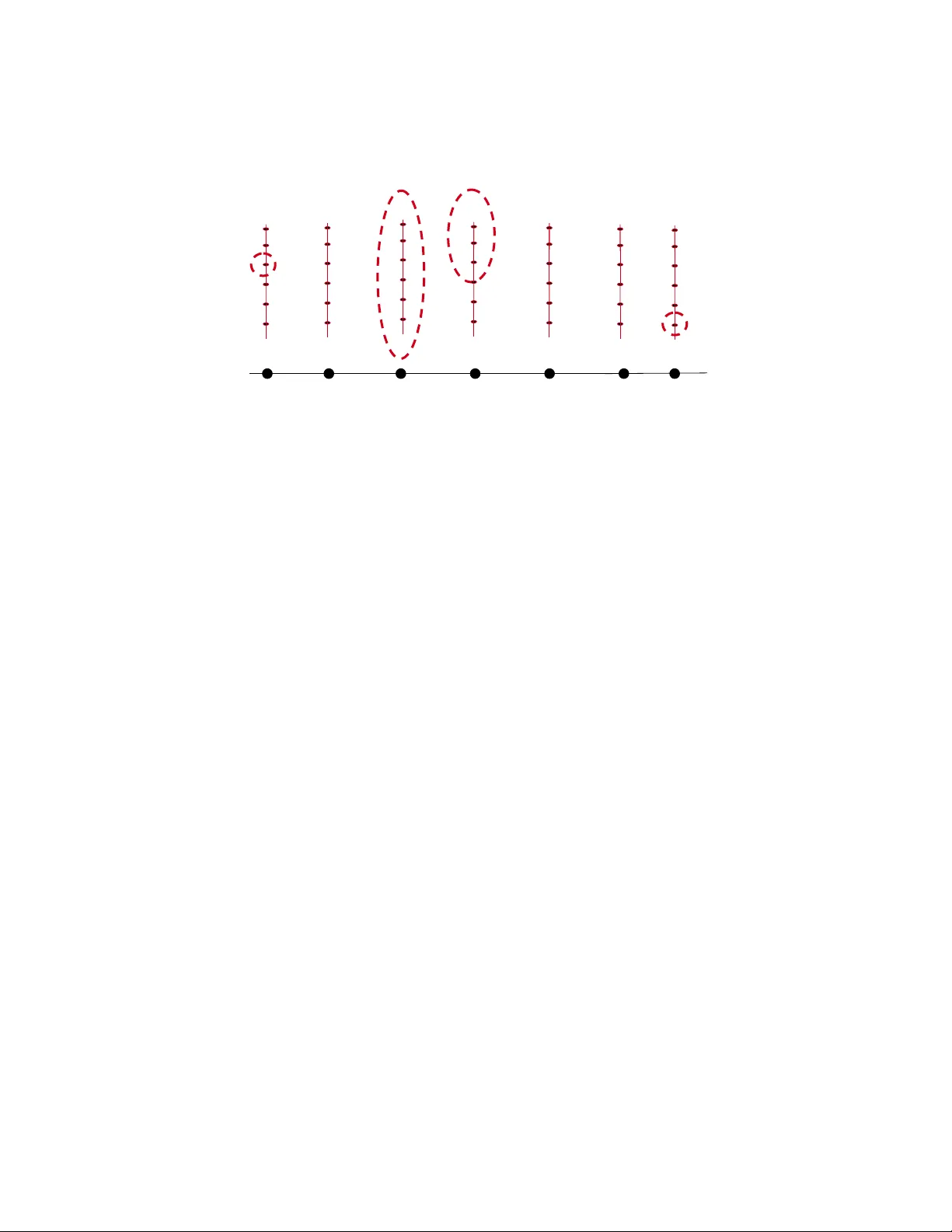
QUANTUM CELLULAR A UTOMA T A: THE GR OUP , THE SP A CE, AND THE SPECTR UM MA TTIE JI AND BOWEN Y ANG Abstract. Ov er an arbitrary commutativ e ring R , we dev elop a theory of quantum cellular automata. W e then use algebraic K-theory to construct a space Q ( X ) of quantum cellular automata (QCA) on a given metric space X . In most cases of in terest, π 0 Q ( X ) classiﬁes QCA up to quantum circuits and stabilization. Notably , the QCA spaces are related b y homotop y equiv alences Q ( ∗ ) ≃ Ω n Q ( Z n ) for all n , whic h sho ws that the classiﬁcation of QCA on Euclidean lattices is given by an Ω-sp ectrum indexed by the dimension n . As a corollary , we also obtain a non-connective delo oping of the K-theory of Azumay a R -algebras, which may b e of independent in terests. W e also include a section leading to the Ω-spectrum for QCA o ver C ∗ -algebras with unitary circuits. T able of Contents 1. In tro duction 2 1.1. Quan tum Cellular Automata 2 1.2. Algebraic K-Theory and Group Completion 3 1.3. Main Results and Outline 4 2. The Quantum Cellular Automata Group 5 2.1. Quan tum Spin System 5 2.2. Quan tum Circuits 9 2.3. Relation to Azumay a algebra 12 2.4. Classiﬁcation is Ab elianization 17 3. The inﬁnite lo op space of spin systems and QCA 18 3.1. Constructing the QCA Space 19 3.2. π 1 and Plus Constructions 20 3.3. π 0 and Coarse Homology Groups 22 4. Delo oping and the Omega-Spectrum 28 5. The QCA Conjecture ov er C ∗ -Algebras with Unitary Circuits 37 5.1. The ∗ -QCA Group 38 5.2. The ∗ -QCA Space 39 5.3. The ∗ -QCA Sp ectrum 40 6. Calculations ov er P oin ts and Lines 40 6.1. Ov er Poin ts and Lines 41 6.2. Rationalization of K 1 43 App endix A. Coarse homology theory 46 App endix B. Group Completion 48 References 50 2020 Mathematics Subje ct Classiﬁc ation. Primary: 19D23, 81P45. Secondary: 55P47. 1 2 MA TTIE JI AND BOWEN Y ANG 1. Introduction 1.1. Quan tum Cellular Automata. Quan tum cellular automata (QCA) origi- nate in quan tum many-bo dy ph ysics and quantum information as locality-preserving automorphisms of the C ∗ -algebras associated to quan tum spin systems. They pro- vide a mathematically precise framework for studying reversible dynamics con- strained by the large-scale geometry of the system. Among the man y problems surrounding QCA, the classiﬁcation problem has attracted the most atten tion. Early progress resulted in the complete classiﬁcation in one dimension [Gro+12]. What follow ed w as a p eriod of rapid progress. W e men tion only a few of the many dev elopmen ts. The group-theoretic foundation was laid out [FH20; FHH22]. Highly non trivial examples were constructed [HFH23; CH23; Shi+22]. A sp ecial class of QCA, known as Cliﬀord QCA, was classiﬁed using algebraic L -groups [Haa25; Y an25]. Connections with top ological ﬁeld theory ha ve b egun to emerge [FHH24; Sun+25], and a bulk–b oundary correspondence was established and related to comm uting Hamiltonian mo dels [R Y25; Haa23; Haa21]. Last but not least, exciting connections to lattice anomalies and inv ertible states ha ve been discov ered [KS25b; F en+25; KS25a; KX25; CGT25; TLE25]. P erhaps the most surprising aspect of the classiﬁcation problem, and what drew the authors’ atten tion, is its connection to homotopy theory . An early hint of this connection app eared in an app endix of a pap er [F re+22] on manifold top ology , but it profoundly inﬂuenced our p erspective. Several prop osals for the homotop y type of QCA ha v e appeared in the physics literature, including formulations in terms of crossed n -cub es [KS25a; KX25] and in the language of ∞ -categories [CGT25; TLE25]. There is no w a folklore conjecture, whic h we refer to as the QCA con- jecture : underlying the classiﬁcation of QCA is an Ω-sp ectrum indexed by the spatial dimension of the lattice Z n . These dev elopmen ts share a common feature: the tec hniques in v olv ed are largely algebraic and, in man y cases, do not rely on the c hoice of base ﬁeld C or on the C ∗ -algebraic structure. Therefore, w e raise the question of whether one can develop a theory of “QCA” ov er an arbitrary comm utative base ring. Moreov er, do es there exist, for eac h suc h ring, an asso ciated Ω-sp ectrum go v erning the classiﬁcation of QCA’s? W e refer to this statemen t as the algebraic QCA hypothesis . In this pap er, we dev elop the theory from ﬁrst principles and prov e the algebraic QCA hypothesis. In doing so, w e construct a family of Ω-sp ectra, one for each comm utative ring. More sp eciﬁcally , for eac h ring R w e ha v e a sequence of inﬁnite lo op spaces: (1.1) Q ( ∗ ) ≃ Ω Q ( Z 1 ) , Q ( Z 1 ) ≃ Ω Q ( Z 2 ) , ..., Q ( Z n − 1 ) ≃ Ω Q ( Z n ) , ... . W e prov e that Q ( Z 1 ) coincides with a space known as the algebr aic K -the ory of Azumaya algebr as over R [W ei81a], but little is known ab out the delooping Q ( Z n ) for general n . It is conjectured, supported by arguments using top ological phases of mat- ter [Haa21; FHH24; Sun+25], that when R = C , the group 1 π 0 Q ( Z 3 ) is equal or ‘close to’ the Witt group of braided fusion C -linear categories [Dav+10; DNO13]. 1 More precisely , the conjecture applies to the original formulation in physics which we discuss in Section 5. QUANTUM CELLULAR AUTOMA T A: THE GROUP , THE SP ACE, AND THE SPECTR UM 3 This leads to another question: o ver a ﬁeld R = k , do es the group π 0 Q ( Z 3 ) repro duce the Witt group of braided fusion k -linear categories? Part of our mo- tiv ation for dev eloping the theory o v er general rings is to even tually understand what QCA detects ab out the ring and to answ er these questions. 1.2. Algebraic K-Theory and Group Completion. Over a ring R , the strategy w e use to construct the QCA spaces Q ( Z n ) is via algebr aic K-the ory and gr oup c ompletion . Algebraic K-theory , on a high lev el, is the study of how to break and assemble ob jects apart linearly , which mak es them amenable to classiﬁcation questions. Giv en a ring R , its K 0 -group is deﬁned as the algebraic group completion of a certain comm utativ e monoid associated to R , and K 0 ( R ) is used to classify ﬁnitely generated pro jective mo dules ov er R . Quillen deﬁned mo dels for higher K-groups [Qui72; Qui73; Gra76] based on the principle that the higher K-theories K i ( R ) of R should b e the homotopy groups π i ( K ( R )) of a space K ( R ), with K 0 ( R ) = π 0 ( K ( R )). Segal [Seg74] constructed a mo del for K ( R ) as the top ological group completion of a topological/homotopical v ersion of a monoid. In particular, Segal’s construction applies to any symmetric monoidal category C and pro duces a corresp onding K-theory space K ( C ). Instead of going up, Bass [Bas68] deﬁned the low er K-groups (also known as negativ e K-groups) K − i ( R ) of a ring R . Pederson show ed [P ed84] that K − i ( R ) can b e reco v ered as π 1 K ( C i +1 ( R )), where C i +1 ( R ) is a symmetric monoidal category asso ciated to R . T o give an informal description of this category C i +1 ( R ) (see [P ed84; PW85]), an ob ject in C i +1 ( R ) is created b y placing a ﬁnitely generated free R -mo dule on eac h p oin t of the lattice Z i +1 ⊂ R i +1 . A morphism betw een t wo ob jects is an R -linear isomorphism that is “uniformly b ounded” with resp ect to the metric on Z i +1 , i.e., there is a uniformly b ounded propagation. The category C i +1 ( R ) is symmetric monoidal under p oin twise direct sum. Pederson and W eib el [PW85] then show ed that these negative K-groups are the homotop y groups of a non-connectiv e delo oping of K ( R ) in to an Ω-sp ectrum. As we will see more formally in Section 2, the precise set-up of QCA is really a m ultiplicative analog of the additive set-up for negative K-theory . Indeed, for the lattice Z i +1 ⊂ R i +1 , a quantum spin system is a placemen t of a matrix algebra o ver R on eac h p oin t of the lattice. A morphism b et w een tw o ob jects is a R -algebra isomorphism that is “uniformly b ounded” (this is called lo c ality-pr eserving ) with resp ect to the metric on Z i +1 , and a quantum cellular automaton is an automor- phism of such quantum spin system. Our p erspective is that we can form a category C ( Z i +1 ) (see Section 3) equipp ed with a symmetric monoidal structure of p oin t- wise tensor pro duct. The associated loop space Ω K ( C ( Z i +1 )) of the K-theory space pro duced b y Segal’s machinery is what w e refer to as Q ( Z i +1 ), the sp ac e of QCA . In fact, our setting applies to a general metric space with reasonable assumptions. W e sho w in Section 4 that Q ( ∗ ) can b e deloop ed in to an Ω-sp ectrum as in (1.1). F urthermore, the term Q ( Z ) can b e iden tiﬁed with K (Az( R )), where Az( R ) denotes the symmetric monoidal category of Azuma y a algebras o v er R . Giv en the close analogy of QCA to negativ e K-theory , the groups π 0 Q ( Z n ) = π 1 K ( C ( Z n )) for n > 1 can b e viewed as “negativ e homotopy groups” to K (Az( R )). This may b e of independent in terest. 4 MA TTIE JI AND BO WEN Y ANG 1.3. Main Results and Outline. The rest of the pap er is organized as follo ws. In Section 2, w e in tro duce the total QCA group Q ( X ) ov er a ring R . The classiﬁcation of QCA on X amounts to computing the quotient Q ( X ) / C ( X ), where C ( X ) is the normal subgroup of quantum circuits. Let X = Z with the usual metric; our ﬁrst theorem connects the classiﬁcation of QCA to that of Azumay a algebras. Theorem 1. Ther e is an explicit surje ctive homomorphism (1.2) b : Q ( Z ) → K 0 (Az(R)) with C ( Z ) = k er b . In Section 3, we deﬁne a symmetric monoidal category C ( X ) of quantum spin systems and use Segal’s K -theory to obtain the QCA space Q ( X ) := Ω( K ( C ( X ))). The homotop y type of K ( C ( X )) admits a description in terms of Quillen’s plus- construction [Qui72]. Theorem 2. K ( C ( X )) ≃ K 0 ( C ( X )) × B Q ( X ) + . In p articular, Q ( X ) ≃ Ω( B Q ( X ) + ) . Com bining Theorem 2 with additional results in Section 2.4, we deduce the relation b et w een Q 0 ( X ) := π 0 Q ( X ) and the QCA classiﬁcation group Q ( X ) / C ( X ) in most cases of in terest, thereb y justifying the name “QCA space.” Corollary 3. F or an y R the following are true. (1) F or n > 0, Q 0 ( Z n ) = K 1 ( C ( Z n )) = Q ( Z n ) ab = Q ( Z n ) / C ( Z n ). (2) Q 0 ( Z ) = K 0 (Az( R )). (3) F or a ﬁeld R satisfying ( R × ) n = R × for all n , Q 0 ( X ) = Q ( X ) / C ( X ) . F or a suitably w ell-b eha ved commutativ e ring R , we also compute K 0 ( C ( X )) and sho w that it is canonically isomorphic to C H 0 ( X, Z ⊕ ω ), the zeroth coarse homology group of X in co eﬃcien t Z ⊕ ω , Here, Z ⊕ ω is the coun tably inﬁnite direct sum of Z . This information is lost after taking the lo op space, but we actually will sho w that K ( C ( Z n )) is connected (i.e., there is no π 0 -information) for n > 0. This is implied b y the following theorem. Theorem 4. L et R b e a ring with no non-trivial idemp otent elements. The gr oup c ompletion of π 0 ( B C ( X )) is c anonic al ly isomorphic to C H 0 ( X, Z ⊕ ω ) . It fol lows that K 0 ( C ( X )) = C H 0 ( X ; Z ⊕ ω ) . In fact, following the proof of Theorem 4, one can show that K ( C ( Z n )) is con- nected for n > 0 ov er an y comm utativ e ring R (see Remark 54). W e then verify in Section 4 that the QCA space w e construct on Euclidean lattices Z n satisﬁes the desired delo oping relation, thereb y proving the algebraic QCA hypothesis. Theorem 5 (The Algebraic QCA Hypothesis) . Ther e is a homotopy e quivalenc e (1.3) Q ( Z n − 1 ) ≃ Ω Q ( Z n ) , for n > 0 . In fact, a similar delooping holds betw een Q ( X ) ≃ Ω Q ( X × Z ) for a giv en metric space X of interest. Section 5 applies our strategy to construct an Ω-sp ectrum for QCA ov er C ∗ - algebras with R = C . In this setting, automorphisms are additionally required to b e C ∗ -algebra maps. This resolves the original formulation of the QCA conjecture in the physics literature. QUANTUM CELLULAR AUTOMA T A: THE GR OUP , THE SP ACE, AND THE SPECTR UM 5 Finally , in Section 6, we compute the homotopy groups of Q ( ∗ ) and Q ( Z ) ov er a ﬁeld. As w e show ed that Q ( Z ) can b e identiﬁed with K (Az( R )), we note the latter has b een computed in [W ei81a]. Here, we pro vide an expository account of the computation o ver a ﬁeld. Appendix A in tro duces some background on coarse homology groups, and App endix B recalls group completion and pro v es a tec hnical lemma ab out it that is used in the main paper. Con v en tions and Notations. Throughout the pap er, the Cartesian product of metric spaces is equipp ed with the L ∞ -metric. All commutativ e rings R are as- sumed to b e unital. Any subalgebra is understo od to b e unital, i.e., to share the same unit as the ambien t algebra. W e write Mat( R n ) for the algebra of n × n matrices ov er R , whic h we refer to as a ful l matrix algebr a (or simply a matrix algebr a ). W e denote b y Mat R the group oid of full matrix algebras o v er R , and by Az( R ) the group oid of Azumay a R -algebras. Ac kno wledgemen t. W e thank Jonathan Blo c k for his hospitalit y at P enn during BY’s visit and for in troducing the tw o authors to each other. W e are grateful to Michael F reedman for his foundational w ork on QCA, which strongly shap ed our persp ectiv e. W e thank Daniel Krashen for helpful discussions on algebraic details, especially concerning Lemma 25, Lemma 28, Corollary 29, Lemma 30, and Lemma 47. W e thank Agn ` es Beaudry for extensive comments and suggestions on the early draft. MJ thanks Mark Behrens and Mona Merling for man y helpful conv ersations and their extensive supp ort throughout this pro ject. MJ also thanks Michael F reed- man for the invitation to sp eak at Harv ard’s F reedman Seminar, Shane Kelly for discussions related to Section 6 and for p oin ting out Remark 94, and Peter Ma y for discussions concerning [May77]. MJ thanks Charles W eib el for helpful con v er- sations, particularly regarding [Bas68; Ma y77; W ei81a; W ei81b; PW85], and for helpful comments on the early draft. BY thanks Mic hael Hopkins and Anton Kapustin for extensiv e discussions and encouragemen t throughout this pro ject. BY is indebted to Shmuel W ein b erger for in tro ducing him to the w ork of P edersen and W eib el during a visit to Chicago, whic h Shmuel kindly arranged. BY also thanks Agn ` es Beaudry , Ulrich Bunke, Dan F reed, and T omer Schlank for stimulating conv ersations. Last but not least, BY b eneﬁted from Mik e’s c ho colate and jok es on numerous occasions. MJ is partially supported b y the National Science F oundation Graduate Researc h F ellowship (DGE-2236662). BY ac kno wledges support from the Simons F oundation through the Simons Collab oration on Global Categorical Symmetries. 2. The Quantum Cellular Automa t a Group In this section, we introduce a setup that leads to a notion of QCA ov er any comm utative ring R . Our deﬁnitions are new, though strongly inspired b y the original formulations in physics. When R = C , the resulting notion diﬀers from the original deﬁnition in that w e do not imp ose a ∗ -algebra structure. In Section 5, w e discuss the original deﬁnition of QCA. 2.1. Quan tum Spin System. Let R b e a commutativ e ring with identit y and ( X, ρ ) be a metric space. W e use N to denote the set of p ositiv e in tegers. 6 MA TTIE JI AND BO WEN Y ANG Deﬁnition 6. A functions q : X → N is called lo cally ﬁnite if (2.1) Λ = { x ∈ X : q x > 1 } is a lo cally ﬁnite subset of X . That is, the intersection betw een Λ and any bounded subset of X is ﬁnite 2 . F requently , Λ is called a ‘lattice’. Denote the collection of suc h functions by N X lf . It is a partially ordered set with q ≤ r if and only if q x | r x for all x ∈ X . T o motiv ate the next deﬁnition, we note that N under m ultiplication is a com- m utative monoid. Moreov er, N can b e identiﬁed with the monoid of isomorphism classes of full matrix algebras o v er R under tensor product by q ∈ N 7→ Mat( R q ) , where Mat( R q ) is the ring of q × q matrices ov er R . Deﬁnition 7. An R -quantum spin system consists of a commutativ e ring R , a metric space ( X, ρ ), and a locally ﬁnite function q ∈ N X lf . Its algebr a of lo c al observables is deﬁned as (2.2) A ( X, q ) = O x ∈ X Mat( R q x ) = lim − → B ⊂ X b ounded O x ∈ B Mat( R q x ) . The tensor pro ducts are tak en ov er R . W e elaborate on the deﬁnition. Let P 0 (Λ) denote the set of ﬁnite subsets of Λ. F or Γ ∈ P 0 (Λ) deﬁne (2.3) A (Γ , q ) := O x ∈ Γ Mat( R q x ) , whic h is a ﬁnite tensor pro duct o v er R . F or an y Y ⊂ X b ounded, Y ∩ Λ ∈ P 0 (Λ) b ecause of lo cal ﬁniteness of q . Deﬁne the algebra of observables supp orte d on Y as (2.4) A ( Y , q ) = A ( Y ∩ Λ , q ) . If Γ ⊂ Γ ′ are ﬁnite subsets, deﬁne the inclusion (2.5) ι Γ , Γ ′ : A (Γ , q ) − → A (Γ ′ , q ) , ι Γ , Γ ′ ( A ) = A ⊗ Id Γ ′ \ Γ , where Id Γ ′ \ Γ is the identit y element in A (Γ ′ \ Γ , q ). Then {A (Γ , q ) } Γ ∈P 0 ( X ) forms a directed system. F or any Z ⊂ X not necessarily b ounded, deﬁne the inductive limit (2.6) A ( Z, q ) = lim − → Γ ∈P 0 (Λ ∩ Z ) A (Γ , q ) . In particular, (2.7) A ( X, q ) = lim − → Γ ∈P 0 (Λ) A (Γ , q ) . In ph ysical applications, the index set Λ is alwa ys countable. W e therefore restrict atten tion to metric spaces X with the prop ert y that every lo cally ﬁnite subset is countable. Typical examples include b ounded metric spaces, Z n , R n , and other second countable metric spaces, such as Riemannian manifolds. 2 In particular, Λ is ﬁnite if M is b ounded. QUANTUM CELLULAR AUTOMA T A: THE GR OUP , THE SP ACE, AND THE SPECTR UM 7 Remark 8. Algebras of this t ype ha v e been studied under the name sup ernatur al matrix algebr as [Bar+23b; Bar+23a]. Under our assumption, the algebra A ( X, q ) ma y b e realized as a c ountable direct limit. Fix an enumeration Λ = { λ 1 , λ 2 , λ 3 , . . . } . Then the increasing chain of ﬁnite subsets { λ 1 } ⊂ { λ 1 , λ 2 } ⊂ { λ 1 , λ 2 , λ 3 } ⊂ · · · is coﬁnal in P 0 (Λ). Consequently , the directed sys tem deﬁning A ( X , q ) may b e computed along this sequence, and A ( X, q ) is the corresp onding countable direct limit. Section 9 of [Bar+23a] is esp ecially relev ant for the analysis of this countable direct-limit. An y tw o systems giv en by q and q ′ stack to a new system giv en by their p oin t- wise product q · q ′ . F urthermore, w e ﬁx a concrete algebra isomorphism Φ betw een A ( X, q ) ⊗ A ( X , q ′ ) and A ( X , q · q ′ ) given point-wise b y the Kroneck er product. Deﬁnition 9. F or p ositiv e in tegers q x , q ′ x , the Kr one cker pr o duct isomorphism (2.8) Φ x : Mat( R q x ) ⊗ Mat( R q ′ x ) − → Mat( R q x q ′ x ) is deﬁned by (2.9) Φ x ( A ⊗ B ) :=      a 11 B a 12 B · · · a 1 q x B a 21 B a 22 B · · · a 2 q x B . . . . . . . . . . . . a q x 1 B a q x 2 B · · · a q x q x B      , where A = ( a ij ) ∈ Mat( R q x ) , B ∈ Mat( R q ′ x ) . Let Φ x b e the iden tit y if either q x = 1 or q ′ x = 1. Remark 10 (Inv erse map) . Giv en C ∈ Mat( R q x q ′ x ), write it as a q x × q x blo c k matrix C =      C 11 C 12 · · · C 1 q x C 21 C 22 · · · C 2 q x . . . . . . . . . . . . C q x 1 C q x 2 · · · C q x q x      , C ij ∈ Mat( R q ′ x ) . Then the inv erse map Φ − 1 x : Mat( R q x q ′ x ) → Mat( R q x ) ⊗ Mat( R q ′ x ) is given b y Φ − 1 x ( C ) = q x X i,j =1 E ( q x ) ij ⊗ C ij , where E ( q x ) ij is the matrix unit in Mat( R q x ). T o deﬁne the equiv alence of quantum spin systems, we need the notion of locality- preserving isomorphism. Deﬁnition 11. Given tw o R -quantum spin systems q , q ′ o ver a metric space ( X, ρ ), a lo c ality-pr eserving homomorphism (resp ectiv ely , isomorphism ) is an R -algebra homomorphism (resp ectiv ely , isomorphism) α : A ( X, q ) − → A ( X , q ′ ) 8 MA TTIE JI AND BO WEN Y ANG of ﬁnite spread. That is, there exists l > 0 such that for ev ery x ∈ X and every A ∈ A ( { x } , q ) = Mat( R q x ) , w e hav e α ( A ) ∈ A ( D x ( l ) , q ′ ) , D x ( l ) := { y ∈ X : d ( x, y ) ≤ l } . A spin system equipped with a lo calit y-preserving automorphism ( q, α ) is called a quantum c el lular automaton (QCA). F or ﬁxed q , the set of QCA forms a group under comp osition, denoted Q ( X, q ). Lo calit y-preserving isomorphisms deﬁne an equiv alence relation betw een spin systems. Whether tw o spin systems are equiv alen t is closely tied to the coarse homology of the underlying metric space ( X , ρ ) and, in man y cases, is indep en- den t of the choice of R . The precise relationship is established in Section 3, and App endix A pro vides a brief ov erview of coarse homology theory . In practice, this p ersp ectiv e allows us to identify a quantum spin system on a space X with one deﬁned on a countable subset of X ha ving the same large-scale geometry . Here, we illustrate this principle with several represen tativ e examples. Example 12. Let X b e a bounded metric space and ﬁx a p oin t x 0 ∈ X . Any spin system q on X is equiv alen t to the spin system q ′ deﬁned by q ′ x 0 = Y x ∈ X q x < ∞ , q ′ x ′ = 1 for x ′  = x 0 . Example 13. Let X = R . Any spin system q on R is equiv alent to the spin system q ′ deﬁned by q ′ n = Y ⌊ x ⌋ = n q x < ∞ for eac h n ∈ Z , and q ′ x ′ = 1 for x ′ / ∈ Z . Lemma 14. The Kroneck er pro duct induces a canonical inclusion (2.10) ι q → r : Q ( X, q )  → Q ( X , r ) , for any q, r ∈ N X lf with q | r . Pr o of. W rite r = q · q ′ . Given a QCA α : A ( X , q ) → A ( X , q ), deﬁne (2.11) ˜ α = Φ ◦ ( α ⊗ id) ◦ Φ − 1 : A ( X, q · q ′ ) → A ( X, q · q ′ ) , where id is the identit y automorphism on A ( M , q ′ ) . □ This inclusion, called stabilization , allo ws comp osition b etw een QCA deﬁned on spin systems with distinct q . One could also stac k tw o locality-preserving isomor- phisms α and β and create an isomorphism on the stac k ed systems. W e will often suppress the conjugation b y Φ, writing α ⊗ β in place of Φ ◦ ( α ⊗ β ) ◦ Φ − 1 when stac king tw o locality-preserving isomorphisms. Deﬁnition 15. The total QCA gr oup is the direct limit in the category of groups: Q ( X ) := lim − → q ∈ N X lf Q ( X, q ) . Concretely , Q ( X ) is the set of equiv alence classes [ q , α ] with α ∈ Q ( X , q ), mo dulo [ q , α ] ∼ [ r, β ] ⇐ ⇒ ∃ s with q | s, r | s suc h that ι q → s ( α ) = ι r → s ( β ) . QUANTUM CELLULAR AUTOMA T A: THE GR OUP , THE SP ACE, AND THE SPECTR UM 9 The pro duct is [ q , α ] · [ r, β ] :=  s, ι q → s ( α ) ◦ ι r → s ( β )  , s x = lcm( q x , r x ) . Sometimes, we write Q ( X ; R ) to emphasize the base ring R . 2.2. Quan tum Circuits. W e record several imp ortant subgroups of Q ( X ). Al- though their elemen ts admit simple descriptions, they represen t a rich class of QCA and are widely studied in quantum information and quan tum many-bo dy ph ysics. W e also observe that each of these subgroups contains the commutator subgroup [ Q ( X ) , Q ( X )] of Q ( X ), a fact that will b e particularly relev an t in later sections. Deﬁnition 16. Let q ∈ N X lf b e a spin system. A single-layer cir cuit consists of: (1) A uniformly b ounded partition X = a j X j , sup j diam( X j ) < ∞ , and we deﬁne q ( X j ) := Y x ∈ X j q x . (2) F or each X j , a choice of automorphism α j of one of the following types: • General automorphism: α j ∈ Aut R A ( X j , q ) ∼ = Aut R Mat( R q ( X j ) ) , • Inner automorphism: α j ∈ PGL q ( X j ) ( R ) , i.e. conjugation by an in v ertible matrix. • Sp ecial linear automorphism: α j ∈ PSL q ( X j ) ( R ) , i.e. conjugation by a matrix of determinant one. • Elemen tary automorphism: α j ( A ) = E AE − 1 for some elementary matrix E . The pro duct Q j α j deﬁnes a lo cality-preserving automorphism of A ( X , q ) b y acting indep endently on the disjoin t tensor factors of A ( X, q ). Figure 1 illustrates a single block in a single-lay er circuit. W e denote by Q ( X, q ) ⊇ C ( X , q ) ⊇ C inn ( X, q ) ⊇ C sp ( X, q ) ⊇ C el ( X, q ) the subgroups generated by single-lay er circuits of the corresp onding gate types. P assing to the direct limit in q , we obtain Q ( X ) ⊇ C ( X ) ⊇ C inn ( X ) ⊇ C sp ( X ) ⊇ C el ( X ) . Remark 17. Ov er the complex n umbers, one could also consider circuits built from unitary matrices. In fact, these are what quantum circuits commonly refer to. See Section 5 for details. 10 MA TTIE JI AND BO WEN Y ANG − 1 0 1 2 − 2 ... ... X = Z Mat( R q 0 ) Mat( R q 1 ) Mat( R q 2 ) Mat( R q − 2 ) Mat( R q − 1 ) M at ( R a ) | {z } ⊗ M at ( R b ) | {z } = Mat( R q − 2 ) = Mat( R a ) ⊗ Mat( R c ) Mat( R q 1 ) = Mat( R b ) ⊗ Mat( R d ) Figure 1. An example of a single blo ck in a gate. Here we break Mat( R q 0 ) into its tw o tensor factors Mat( R a ) and Mat( R b ), w e then swap out the corresp onden t tensor comp onents Mat( R a ) ⊆ Mat( R q − 2 ) and M at ( R b ) ⊆ Mat( R q 1 ) to p erform the automor- phism. Example 18. Here w e giv e an example of elemen tary quantum circuits. F or a spin system q · r , there are tw o factorizations based on the (in v erse) Kronec k er pro duct (2.12) A ( X, q · r ) ∼ = A ( X, q ) ⊗ A ( X , r ) ∼ = A ( X, r ) ⊗ A ( X, q ) , one can deﬁne the SW AP q ,r : A ( X, q ) ⊗ A ( X, r ) → A ( X , r ) ⊗ A ( X, q ) circuit which switc hes b etw een these tw o orderings ab ov e. Sp eciﬁcally , it is the partition of X in to individual p oints, and on eac h point we hav e an automorphism by the follo wing form ula (2.13)      a 11 B a 12 B · · · a 1 q x B a 21 B a 22 B · · · a 2 q x B . . . . . . . . . . . . a q x 1 B a q x 2 B · · · a q x q x B      7→      b 11 A b 12 A · · · b 1 r x A b 21 A b 22 A · · · b 2 r x A . . . . . . . . . . . . b r x 1 A b r x 2 A · · · b r x r x A      for each A = ( a ij ) ∈ Mat( R q x ) and B = ( b ij ) ∈ Mat( R r x ). After stabilization, a SW AP automorphism is alwa ys equal to a conjugation by an elementary matrix. Indeed, the SW AP automorphism is the conjugation b y a p ermutation matrix that is stably ev en (see [Liu+24] for a pro of of this), and even p ermutation matrices are elemen tary (see I I I.1.2.1 of [W ei13]). Example 19. F or X = ∗ is a p oint, w e hav e that Q ( ∗ ) = C ( ∗ ). Prop osition 20. Each of the four circuit subgroups is normal in Q ( X ). Pr o of. Let α = Q j ∈ J α j b e a single-lay er (inner, sp ecial, or elementary) circuit, with each α j an automorphism of A ( X j , q ) b elonging to the corresp onding gate- t yp e. Recall that (2.14) X = a j ∈ J X j and sup j ∈ J diam( X j ) < ∞ . QUANTUM CELLULAR AUTOMA T A: THE GR OUP , THE SP ACE, AND THE SPECTR UM 11 F or an y β ∈ Q ( X , q ) of spread l , β ◦ α j ◦ β − 1 is an automorphism of the same gate-t yp e on A ( X l j , q ) with (2.15) X l j = { x ∈ X : d ( x, X j ) ≤ l } . Ab o ve, w e are regarding α j as an automorphism of the en tire algebra A ( X, q ) whic h acts as identit y outside X j . In other w ords, (2.16) β ◦ α ◦ β = Y j β ◦ α j ◦ β − 1 where the factors are mutually commuting but may ov erlap in supp ort. Though not a single-la yer circuit an ymore, β ◦ α ◦ β is still a (multi-la y er) circuit of the same t yp e. Indeed, one can stagger the terms in the product and regroup them so that op erators with disjoint support are assigned to the same lay er. □ Prop osition 21. The quotient group Q ( X ) / C el ( X ) is abe lian. In other words, [ Q ( X ) , Q ( X )] ⊂ C el ( X ) . Pr o of. Let α ∈ Q ( X, q ) and β ∈ Q ( X , r ). Within the total QCA group Q ( X ), [ q , α ][ r, β ] =[ q r, α ⊗ id r ][ q r, SW AP q ,r ][ q r, id q ⊗ β ][ q r, SW AP q ,r ] =[ q r, α ⊗ id r ][ q r, id q ⊗ β ][ q r, id q ⊗ β − 1 ][ q r, SW AP q ,r ][ q r, id q ⊗ β ][ q r, SW AP q ,r ] =[ q r, id q ⊗ β ][ q r, α ⊗ id r ][ q r, id q ⊗ β − 1 ][ q r, SW AP q ,r ][ q r, id q ⊗ β ][ q r, SW AP q ,r ] =[ r , β ][ q , α ][ q r, id q ⊗ β − 1 ][ q r, SW AP q ,r ][ q r, id q ⊗ β ][ q r, SW AP q ,r ] . Since both [ q r, id q ⊗ β − 1 ][ q r, SW AP q ,r ][ q r, id q ⊗ β ] and [ qr, SW AP q ,r ] are in C el ( X ) w e are done. □ Corollary 22. The groups Q ( X ) / C ( X ), Q ( X ) / C inn ( X ), and Q ( X ) / C sp ( X ) are also ab elian. Prop osition 23. Let β b e a lo calit y-preserving isomorphism α b etw een q and q ′ . A QCA [ q , α ] ∈ Q ( X ) and its conjugate [ q ′ , β αβ − 1 ] are equiv alent in Q ( X ) ab . Hence they are also equiv alent in Q ( X ) / C ( X ), Q ( X ) / C inn ( X ), Q ( X ) / C sp ( X ), and Q ( X ) / C el ( X ). Pr o of. The comp osition ˜ β := SW AP q ′ , q ◦ ( β ⊗ β − 1 ) : A ( X, q ) ⊗ A ( X , q ′ ) → A ( X, q ) ⊗ A ( X , q ′ ) giv es a QCA on qq ′ . Notice, ˜ β ◦ ( α ⊗ Id ′ q ) ◦ ˜ β − 1 (2.17) =SW AP q ′ , q ◦ ( β ⊗ β − 1 ) ◦ ( α ⊗ Id q ′ ) ◦ ( β − 1 ⊗ β ) ◦ SW AP q , q ′ (2.18) =Id q ⊗ ( β αβ − 1 ) , (2.19) where the ﬁrst iden tity is on A ( X , q ′ ) and the last on A ( X , q ) . Therefore, in the ab elianization Q ( X ) ab , (2.20) [ q , α ] = [ q q ′ , α ⊗ Id ′ q ] = [ q q ′ , Id q ⊗ ( β αβ − 1 )] = [ q ′ , β αβ − 1 ] . □ 12 MA TTIE JI AND BO WEN Y ANG 2.3. Relation to Azumay a algebra. Recall that an R -algebra A is called an Azumaya algebr a if there exists another R -algebra B such that A ⊗ R B ∼ = Mat( R n ) for some n . Azuma y a algebra ov er R form a symmetric monoidal category Az(R) under tensor pro duct. Let K 0 (Az(R)) b e its Grothendieck group whose elements are represented by fractions of the form A B . Here, A, B are Azuma y a algebras. If P is a faithfully pro jective 3 R -mo dule, then End R ( P ) is an Azuma ya algebra. Since End R ( P ⊗ P ′ ) ∼ = End R ( P ) ⊗ End R ( P ′ ) , there is a monoidal functor End R : FP( R ) − → Az( R ) , where FP( R ) denotes the monoidal category of ﬁnitely generated faithfully pro jec- tiv e R -mo dule with tensor pro duct. Hence, we obtain a group homomorphism K 0 (FP( R )) − → K 0 (Az( R )) . The cokernel Br( R ) of this map is called the Br auer gr oup of R . Thus Br( R ) is generated by classes [ A ] of Azumay a algebras, sub ject to the relations [ A ⊗ R B ] = [ A ] + [ B ] , [End R ( P )] = 0 . Remark 24. A modern deﬁnition of Azumay a R-algebras typically states that A is Azuma y a if there exists an R -algebra B suc h that A ⊗ R B ∼ = End R ( P ), where P is a faithfully pro jective R -mo dule. As p ointed out in Chapter IX.7 of [Bas68], the category of ﬁnitely generated free R -mo dules is actually coﬁnal in FP under tensor pro duct. Hence, the tw o deﬁnitions agree with each other. F or con venience, w e also record a fact about Azuma ya algebras that w e will utilize in later sections. Lemma 25 (The Cen tralizer Theorem) . Let R b e a comm utativ e ring. Let A be a ﬁnite-dimensional Azuma y a R -algebra, and let B ⊆ A b e a unital R -subalgebra whic h is also Azumay a ov er R . Let C := { a ∈ A | ab = ba for all b ∈ B } b e the centralizer of B in A . Then C is an Azumay a R -algebra, and the natural m ultiplication map B ⊗ R C − → A, b ⊗ c 7→ bc, is an isomorphism of R -algebras. In particular, B and C are m utual cen tralizers in A . Pr o of. The multiplication map B ⊗ R C → A is an isomorphism if and only if it is lo cally an isomorphism at eac h prime ideal of R . This reduces to the case of ﬁelds, and the theorem follo ws from the centralizer theorem for ﬁelds (see Lemma 11.7.2 of [Sta26], for example). □ Theorem 1. Ther e is an explicit surje ctive homomorphism (1.2) b : Q ( Z ) → K 0 (Az(R)) with C ( Z ) = ker b . 3 P is a ﬁnitely generated pro jective R -mo dule whose rank at ev ery comp onent of Sp ec( R ) is non-zero. See I I.5.4.2 of [W ei13] for more details. QUANTUM CELLULAR AUTOMA T A: THE GR OUP , THE SP ACE, AND THE SPECTR UM 13 Pr o of. Let [ q , α ] ∈ Q ( Z ) for q ∈ N Z lf and α ∈ Q ( Z , q ) with spread l . Choose an y γ ∈ Z . Informally , we w ould like to deﬁne b ( α ) as (2.21) α ( A ( Z ∩ ( −∞ , γ ] , q )) A ( Z ∩ ( −∞ , γ ] , q ) ∈ K 0 Az(R) . T o make it well-deﬁned, w e use the ﬁnite spread condition, (2.22) A ( Z ∩ ( −∞ , γ − l ] , q )) ⊂ α ( A ( Z ∩ ( −∞ , γ ] , q )) ⊂ A ( Z ∩ ( −∞ , γ + l ] , q )) . Lemma 28 b elow implies (2.23) α ( A ( Z ∩ ( −∞ , γ ] , q )) = A ( Z ∩ ( −∞ , γ − l ] , q ) ⊗ B , where B ⊂ A ( Z ∩ ( γ − l , γ + l ] , q ) is a unital subalgebra. Similarly , (2.24) α ( A ( Z ∩ ( γ , ∞ ) , q )) = C ⊗ A ( Z ∩ ( γ + l , ∞ ) , q ) , where C ⊂ A ( Z ∩ ( γ − l , γ + l ] , q ) is a subalgebra. As α is an algebra automorphism, B ⊗ C = A ( Z ∩ ( γ − l, γ + l ] , q ), elements in B and C commute, and B ∩ C = R . This implies B is Azuma y a. No w the expression for b ( α ) b ecomes (2.25) A ( Z ∩ ( −∞ , γ − l ] , q ) ⊗ B A ( Z ∩ ( −∞ , γ − l ] , q ) ⊗ A ( Z ∩ ( γ − l , γ ] , q ) = B A ( Z ∩ ( γ − l , γ ] , q ) ∈ K 0 Az(R) . The righ t-hand-side is the deﬁnition of b ( α ). Using a diﬀerent l do es not change the v alue as long as it is greater than the spread of α . Since (2.26) α ( A ( Z ∩ ( −∞ , γ + 1] , q )) A ( Z ∩ ( −∞ , γ + 1] , q )) = α ( A ( Z ∩ ( −∞ , γ ] , q )) ⊗ α ( A ( { γ + 1 } , q )) A ( Z ∩ ( −∞ , γ ] , q )) ⊗ A ( { γ + 1 } , q ) , and A ( { γ + 1 } , q ) ∼ = Mat( R q γ +1 ) ∼ = α ( A ( { γ + 1 } , q )), b ( α ) do es not dep end on γ . Stabilization, or Kronec k er product b etw een α and iden tity , does not c hange b ( α ) either. Without loss of generality , let [ q , α ] , [ q , β ] ∈ Q ( Z ) hav e the same q . V erify that b ( β α ) = β α ( A ( Z ∩ ( −∞ , γ ] , q )) A ( Z ∩ ( −∞ , γ ] , q )) = β ( A ( Z ∩ ( −∞ , γ − l ] , q )) ⊗ β ( B ) A ( Z ∩ ( −∞ , γ − l ] , q ) ⊗ A ( Z ∩ ( γ − l , γ ] , q ) = β ( A ( Z ∩ ( −∞ , γ − l ] , q )) A ( Z ∩ ( −∞ , γ − l ] , q ) ⊗ β ( B ) A ( Z ∩ ( γ − l , γ ] , q ) = b ( β ) ⊗ b ( α ) ∈ K 0 Az(R) , where, for the last equality , we used the indep endence of γ and that β ( B ) ∼ = B . Th us, b is a w ell-deﬁned group homomorphism as claimed. T o c hec k that C ( Z ) is in the kernel, simply tak e a single-lay er circuit α = Q α j where α j ’s are automorphisms of algebra supp orted on disjoint b ounded interv als. Cho ose γ to b e the end p oint of one of the in terv als so that α ( A ( Z ∩ ( −∞ , γ ] , q )) = A ( Z ∩ ( −∞ , γ ] , q ) and b ( α ) = 1 . Con versely , if b ( α ) = 1 then B ∼ = A ( Z ∩ ( γ − l, γ ] , q ). Choose an automorphism β 0 ∈ Aut( A ( Z ∩ ( γ − l, γ + l ] , q )) whic h sends B to A ( Z ∩ ( γ − l , γ ] , q ). Then β 0 α is a pro duct of automorphisms on A ( Z ∩ ( −∞ , γ ] , q ) and A ( Z ∩ ( γ , ∞ )) resp ectively . Cho ose similarly for all k ∈ Z β k ∈ Aut( A ( Z ∩ ( γ − (2 k − 1) l , γ + (2 k + 1) l ] , q )) 14 MA TTIE JI AND BO WEN Y ANG and notice β = Q k β k and β α are b oth in C ( Z ). Therefore, α ∈ C ( Z ) . F or surjectivit y , consider the element A B ∈ K 0 (Az( R )) where A and B are both Azuma ya R -algebras. By deﬁnition, there exists R -algebras A ′ and B ′ suc h that A ⊗ A ′ ∼ = Mat( R n ) and B ⊗ B ′ ∼ = Mat( R m ). Now consider the particular QCA α with spin system q illustrated in Figure 2. Now observe that α has spread ≤ 2, and α ( A ( Z ∩ ( −∞ , − 1] , q )) = A ( Z ∩ ( −∞ , − 3] , q ) ⊗ B ′ |{z} on -2 ⊗ A ⊗ A ′ | {z } on -1 ⊗ A |{z} on 1 . Then we ha v e that b ( α ) = B ′ ⊗ A ⊗ A ′ ⊗ A A ( Z ∩ ( − 3 , − 1] , q ) = B ′ ⊗ A ⊗ A ′ ⊗ A B ⊗ B ′ ⊗ A ⊗ A ′ = A B . □ Corollary 26. Every α ∈ C ( Z ) is equal to a composition of at most t w o single-la yer circuits. Pr o of. If b ( α ) = 1, we can rep eat the pro cedure in the pro of abov e to ﬁnd a single- la yer circuit β such that β α is a single-la yer circuit itself. □ − 1 0 1 2 − 2 ... ... B |{z} ⊗ B ′ − 3 A |{z} ⊗ A ′ A |{z} ⊗ A ′ A |{z} ⊗ A ′ B |{z} ⊗ B ′ B |{z} ⊗ B ′ ... ... ... ... Figure 2. A QCA α suc h that b ( α ) = A B ∈ K 0 (Az R ). Here w e place an alternating sequence of A ⊗ A ′ ∼ = Mat( R n ) and B ⊗ B ′ ∼ = Mat( R m ) on Z , and α simultaneously transports the tensor factor B to the left and the tensor factor A to the righ t. W e divide the line b etw een − 1 and 0 in the construction of the elemen t β ( α ). Remark 27. Theorem 1 sho ws that Q ( Z ) / C ( Z ) can b e in terpreted as an alterna- tiv e deﬁnition of K 0 Az( R ). Intuitiv ely , a QCA on Z can b e viewed as pumping an Azuma ya algebra along the chain. F or a general metric space X , an analogous phe- nomenon occurs: a QCA deﬁned on X × Z produces a class of inﬁnite-dimensional R -algebras. These play a role analogous to that of Az uma ya algebras relative to matrix algebras in their relationship with A ( X, q ). See Deﬁnition 60 in Section 4. W e end this subsection with some useful technical lemmas. QUANTUM CELLULAR AUTOMA T A: THE GR OUP , THE SP ACE, AND THE SPECTR UM 15 Lemma 28. Let R be a commutativ e unital ring. Let A and C be unital R -algebras, and regard A as the unital subalgebra A ⊗ R 1 ⊆ A ⊗ R C . Assume that A is a lo c al ly matrix R -algebr a , i.e. there exists a directed system of unital R -subalgebras ( A λ ) λ ∈ Λ with A = [ λ ∈ Λ A λ , A λ ∼ = Mat( R n ( λ ) ) as unital R -algebras. Let B ⊆ A ⊗ R C b e a unital R -subalgebra such that A ⊗ R 1 ⊆ B and 1 B = 1 A ⊗ C . Deﬁne D := { c ∈ C : 1 ⊗ c ∈ B } ⊆ C . Then D is a unital R -subalgebra of C and B = A ⊗ R D ⊆ A ⊗ R C. Corollary 29. The same holds if A is a tensor factor of a lo cally matrix R -algebra with the same identit y element, i.e., there exists a unital R -algebra A ′ with A ⊗ A ′ lo cally matrix. Pr o of. Since B ⊆ A ⊗ R C , A ′ ⊗ R B ⊆ A ′ ⊗ R A ⊗ R C . Apply the lemma, A ′ ⊗ R B = A ′ ⊗ R A ⊗ R D , with D = { c ∈ C : 1 ⊗ 1 ⊗ c ∈ A ′ ⊗ R B } = { c ∈ C : 1 ⊗ c ∈ B } . This directly implies B = A ⊗ R D . □ Pr o of of lemma. It can be v eriﬁed that D is a unital R -subalgebra of C . Moreo ver, w e ha v e ( A ⊗ 1) · (1 ⊗ D ) = A ⊗ D ⊆ B . Th us, it remains to pro v e the reverse inclusion B ⊆ A ⊗ D . Step 1: The ﬁnite matrix case. W e ﬁrst prov e the follo wing claim. Let A 0 = Mat( R n ) and let B 0 ⊆ A 0 ⊗ R C b e a unital R -subalgebra with A 0 ⊗ 1 ⊆ B 0 . If D 0 := { c ∈ C : 1 ⊗ c ∈ B 0 } , then B 0 = A 0 ⊗ R D 0 . Fix a system of matrix units { e ij } 1 ≤ i,j ≤ n ⊆ A 0 . (So e ij e kℓ = δ j k e iℓ and P n i =1 e ii = 1.) Since A 0 ⊗ 1 ⊆ B 0 , we ha v e e ij ⊗ 1 ∈ B 0 for all i, j . Let b ∈ B 0 b e arbitrary . F or each 1 ≤ i, j ≤ n , consider the elemen t x ij := ( e 1 i ⊗ 1) b ( e j 1 ⊗ 1) ∈ B 0 , since B 0 is a subalgebra. Because ( e 1 i ⊗ 1)( A 0 ⊗ C )( e j 1 ⊗ 1) = ( e 1 i A 0 e j 1 ) ⊗ C = e 11 ⊗ C, there exists a unique element c ij ∈ C such that x ij = e 11 ⊗ c ij . In particular e 11 ⊗ c ij ∈ B 0 . W e no w sho w that c ij ∈ D 0 . F or eac h 1 ≤ k ≤ n w e compute, using e k 1 e 11 e 1 k = e kk , ( e k 1 ⊗ 1) ( e 11 ⊗ c ij ) ( e 1 k ⊗ 1) = ( e kk ⊗ c ij ) ∈ B 0 . Summing ov er k yields 1 ⊗ c ij = n X k =1 e kk ! ⊗ c ij = n X k =1 ( e kk ⊗ c ij ) ∈ B 0 , 16 MA TTIE JI AND BO WEN Y ANG hence c ij ∈ D 0 . Finally we reconstruct b from the c ij : n X i,j =1 e ij ⊗ c ij = n X i,j =1 ( e i 1 ⊗ 1)( e 11 ⊗ c ij )( e 1 j ⊗ 1) = n X i,j =1 ( e i 1 ⊗ 1) ( e 1 i ⊗ 1) b ( e j 1 ⊗ 1) ( e 1 j ⊗ 1) = n X i =1 e i 1 e 1 i ⊗ 1 ! b   n X j =1 e j 1 e 1 j ⊗ 1   = n X i =1 e ii ⊗ 1 ! b   n X j =1 e j j ⊗ 1   = (1 ⊗ 1) b (1 ⊗ 1) = b. Since each c ij ∈ D 0 , this shows b ∈ A 0 ⊗ D 0 , hence B 0 ⊆ A 0 ⊗ D 0 . The reverse inclusion A 0 ⊗ D 0 ⊆ B 0 is immediate b ecause A 0 ⊗ 1 ⊆ B 0 and 1 ⊗ D 0 ⊆ B 0 , and their pro ducts generate A 0 ⊗ D 0 . Thus B 0 = A 0 ⊗ D 0 . Step 2: Reduction to the ﬁnite case using the lo cally matrix hypothesis. Let b ∈ B b e arbitrary . As an element of the algebraic tensor pro duct A ⊗ R C , it is a ﬁnite R -linear combination of pure tensors: b = N X t =1 a t ⊗ c t , a t ∈ A, c t ∈ C. Since A = S λ A λ , there exists λ s uc h that a t ∈ A λ for all t , hence b ∈ A λ ⊗ R C . Deﬁne the (unital) subalgebra B λ := B ∩ ( A λ ⊗ R C ) ⊆ A λ ⊗ R C. Then A λ ⊗ 1 ⊆ B λ b ecause A ⊗ 1 ⊆ B and A λ ⊆ A . Apply the claim (Step 1) to A 0 := A λ ∼ = Mat( R n ( λ ) ) and B 0 := B λ . W e obtain B λ = A λ ⊗ R D λ , D λ := { c ∈ C : 1 ⊗ c ∈ B λ } . W e now iden tify D λ with D . Note that 1 ⊗ c ∈ A λ ⊗ C for every λ and ev ery c ∈ C , b ecause 1 ∈ A λ . Hence 1 ⊗ c ∈ B λ ⇐ ⇒ 1 ⊗ c ∈ B and 1 ⊗ c ∈ A λ ⊗ C ⇐ ⇒ 1 ⊗ c ∈ B . Th us D λ = D . Therefore, b ∈ B λ = A λ ⊗ R D ⊆ A ⊗ R D . Since b ∈ B was arbitrary , we conclude B ⊆ A ⊗ R D . □ W e deduce an extended v ersion of the centralizer theorem (Lemma 25). Lemma 30. Let B ⊆ A ⊆ C where C = A ( X , q ). Supp ose A and B are b oth tensor factors of C , then A = B ⊗ ( A ∩ B ′ ). QUANTUM CELLULAR AUTOMA T A: THE GR OUP , THE SP ACE, AND THE SPECTR UM 17 Pr o of. W e hav e that B ⊗ B ′ = C . W e hav e B = B ⊗ R 1 ⊆ A ⊆ B ⊗ R B ′ . Thus, Corollary 29 implies that A = B ⊗ R B ′′ . W e can identify B ′′ , constructed in the corollary , exactly with A ∩ B ′ as A ∩ B ′ is equal to the centralizer of B in A . □ 2.4. Classiﬁcation is Ab elianization. Lastly , w e sho w that, in most cases of in terest, the classiﬁcation group of QCA is given by ab elianizing the total QCA group. This certiﬁes that the classiﬁcation of QCA arises canonically , rather than as an ad ho c construction. Lemma 31. Let k b e a ﬁeld satisfying ( k × ) n = k × for all n (ex. algebraically closed ﬁelds). C ( X ; k ) is equal to the comm utator subgroup of Q ( X ; k ). Pr o of. Since k has n -th ro ots for all n , so PGL n ( k ) = PSL n ( k ), and PSL n ( k ) is sim- ple and hence p erfect for n ≥ 3. The prop osition ab ov e shows that Q ( X ; k ) /C ( X ; k ) is ab elian, so we ha v e that [ Q ( X ; k ) , Q ( X ; k )] ⊆ C ( X ; k ). As we will see later in the pap er, Q ( X ; k ) may b e constructed as Aut( S ) of an appropriate symmetric monoidal category S , and hence its commutator subgroup is its maximal p erfect subgroup. Thus, it suﬃces to show that C ( X ; k ) is p erfect. No w, let Q j α j b e a single-lay er circuit, indexed ov er b ounded X j ’s that form a disjoint partition of X . Up to stabilization, eac h α j is without loss an au- tomorphism of Mat( R q ( X j ) ) where q ( X j ) ≥ 3. Since ( k × ) n = k × for all n , Aut(Mat( R q ( X j ) )) ∼ = PGL q ( X j ) ( R ) ∼ = PSL q ( X j ) ( R ) is p erfect. This means that w e can write α j = x j, 1 ...x j,n j where x j, • is a comm utator. Observe that if the n j ’s can b e made to be uniformly b ounded with resp ect to j , then we are done. Indeed, supp ose we c hoose N ≥ n j for all j , then without loss we can mak e n j = N for all j b y padding the iden tity elemen t, which is also a comm utator. Now for 1 ≤ i ≤ N , write x j,i = z − 1 j,i y − 1 j,i z j,i y j,i , we deﬁne β i := Y j x j,i = ( Y j z − 1 j,i )( Y j y − 1 j,i )( Y j z j,i )( Y j y j,i ) = ( Y j z j,i ) − 1 ( Y j y j,i ) − 1 ( Y j z j,i )( Y j y j,i ) ∈ [ C ( X ; k ) , C ( X ; k )] . Observ e that Q j α j = β 1 ...β N ∈ [ C ( X ; k ) , C ( X ; k )]. This shows that C ( X ; k ) ⊆ [ C ( X ; k ) , C ( X ; k )], and hence C ( X ; k ) is p erfect. As noted ab ov e, there is a subtlety that the n j ’s ma y not b e uniformly b ounded with resp ect to j . F ortunately , by Theorem 1 and 2 of [Tho61] and the fact that PSL n ( k ) is a quotient of SL n ( k ), the n j ’s can b e made to b e uniformly b ounded (in fact, N can b e chosen to b e 2). □ The same pro of ab ov e also shows that. Lemma 32. Let k b e a ﬁeld. C sp ( X ; k ) is equal to the comm utator subgroup of Q ( X ; k ). The iden tiﬁcations ab ov e rely on the ring R we are w orking with. Now w e derive an identiﬁcation that relies on the space rather than the ring. Deﬁnition 33. On metric spaces of the form X × Z , w e say a QCA ( q , α ) blends into the identity if there exists l ∈ Z such that α restricts to identit y on either A ( X × Z ≤ l , q ) or A ( X × Z ≥ l , q ). 18 MA TTIE JI AND BO WEN Y ANG Lemma 34. An y [ q , α ] ∈ Q ( X × Z ) which blends in to iden tit y is in [ Q ( X × Z ) , Q ( X × Z )] . Pr o of. Giv en any QCA [ q , α ], deﬁne its tr anslate [ T q , T α ] b y (2.27) ( T q )( x, n + 1) = q ( x, n ) for all n ∈ Z , with a lo cality-preserving isomorphism (2.28) τ : A ( X × Z , q ) → A ( X × Z , T q ) that identiﬁes A ( X × { n } , q ) with A ( X × { n + 1 } , T q ). Then (2.29) T α := τ ατ − 1 . By Prop osition 23, a QCA and its translate are equal in Q ( X × Z ) ab . No w, given a QCA that restricts to identit y on A ( X × Z ≤ 0 , q ), c ho ose a rep- resen tative [ q , α ] ∈ Q ( X ) for it that satisﬁes q ≡ 1 on X × Z ≤ 0 . This is alwa ys p ossible b ecause of the assumption. The inﬁnite pro duct (2.30) q S := ∞ Y m =0 T m q is a w ell-deﬁned spin system because q S tak es a ﬁnite v alue on ev ery point in X × Z . Therefore, (2.31) " q S , α S := ∞ O m =0 T m α # ∈ Q ( X × Z ) . see Figure 3 for an illustration of q S and α S . W e deduce that in Q ( X × Z ) ab , (2.32) [ T q S , T α S ] = " ∞ Y m =1 T m q , ∞ O m =1 T m α # = [ q S , α S ] , Moreo ver, it is easy to chec k that (2.33) [ q S , α S ] = [ q , α ] · [ T q S , T α S ] . In conclusion, [ q , α ] is trivial in Q ( X × Z ) ab . □ Prop osition 35. On metric spaces of the form X × Z and o v er an y ring R , the four circuit subgroups deﬁned are all equal to the commutator subgroup of Q ( X × Z ). Pr o of. It suﬃces to show that a single-lay er circuit of any type is trivial in the ab elianization Q ( X × Z ) ab . Clearly , a single-lay er circuit α = Q j α j is a pro duct of t wo circuits that blend in to the identit y . The result follows from Lemma 34. □ Note that Prop osition 35 can alternatively follo w from Lemma 59 later, whose pro of follows a similar theme here. 3. The infinite loop sp ace of spin systems and QCA In this section, we will construct a top ological enrichmen t of the total QCA group (Deﬁnition 15). As hinted in the previous section, we will use algebraic K-theory to build suitable spaces that enco de the QCA group. The sp eciﬁc approach we will tak e is to apply Segal’s construction for the algebraic K-theory of a symmetric monoidal category [Seg74]. QUANTUM CELLULAR AUTOMA T A: THE GR OUP , THE SP ACE, AND THE SPECTR UM 19 − 1 0 1 2 − 2 ... ... − 3 3 α ... α ... α ... Figure 3. An illustration of q S and α S app earing in the proof of Lemma 34. The ﬁgure illustrates the case where X is a point. 3.1. Constructing the QCA Space. Before deﬁning our QCA space, w e should ﬁrst sp ecify the symmetric monoidal category w e are working with. Deﬁnition 36. The category of quan tum spin systems is a category C ( X ) whose: • Ob jects are A ( X , q ) for each quan tum spin system q : X → N > 0 . • Morphisms are lo cality-preserving isomorphisms (recall Deﬁnition 11). C ( X ) is symmetric monoidal under the p oint wise stac king op eration deﬁned around Deﬁnition 9. Example 37. Let X = ∗ be a p oint, then C ( ∗ ) is the category Mat R of ma- trix algebras Mat( R n ), with morphisms as R -algebra automorphisms, symmetric monoidal under tensor pro duct. Note that π 0 ( B Mat R ) = Z > 0 is the m ultiplicativ e monoid of p ositive integers, whose group completion is the group of positive ratio- nals Q > 0 under m ultiplication. When R is an algebraically closed ﬁeld such as C , this coincides with Az( R ). Since there is a local ﬁniteness requirement to quantum spin systems, w e see C ( R n ) and C ( Z n ) are equiv alent as symmetric monoidal categories. Recall we also assumed that X has a countable subset Λ. It is reasonable to assume in practice that the inclusion Λ → X is what is called a “coarse equiv alence” (ex. the inclusion Z n → R n , see App endix A for more details), and it follows that C ( X ) and C (Λ) are equiv alent. Thus, for the rest of this section, w e will assume X is a lo cally ﬁnite countable metric space . F or any (small) symmetric monoidal category C , Segal constructs its K-theory space K ( C ) as follows. Deﬁnition 38. Let C b e a (small) symmetric monoidal category , its classifying space B C has the natural structure of a homotopy commutativ e, homotopy asso- ciativ e H -space. In particular, π 0 ( B C ) is a commutativ e monoid. The K-the ory sp ac e K ( C ) is deﬁned as the gr oup c ompletion ι : B C → K ( C ) of B C , which is c haracterized by the follo wing prop erty (1) K ( C ) is a group-like H-space. In particular, π 0 ( K ( C )) is a group. (2) The induced map ι ∗ : π 0 ( B C ) → π 0 ( K ( C )) is the algebraic group completion of the commutativ e monoid π 0 ( B C ). (3) The homology of H ∗ ( K ( C ); R ) is the localization of H ∗ ( B C ; R ) at π 0 ( B C ) for any commutativ e ring R . Here, the homologies are rings b ecause the relev ant spaces are H-spaces. 20 MA TTIE JI AND BO WEN Y ANG The i -th K -theory of C is denoted K i ( C ) : = π i ( K ( C )). The construction is functorial with resp ect to lax symmetric monoidal functors. The group completion may not be unique in some cases, but they are equiv alen t if C has coun tably many ob jects (see Theorem IV.4.4.3 of [W ei13]). The following theorem gives an explicit construction of said group completion. Theorem 39 (The Group Completion Theorem [MS76]) . L et C b e a (smal l) sym- metric monoidal c ate gory. K ( C ) = Ω B ( B C ) is a gr oup c ompletion of B C . K ( C ) is the zeroth space of an Ω-sp ectrum and is an inﬁnite loop space. W e will see later that the QCA group actually corresp onds more closely to in- formation at the level of π 1 . This motiv ates 4 us to apply a lo op space on top of the K-theory space, at the component corresp onding to the identit y element in π 0 . Finally , we deﬁne the QCA space as follo ws. Deﬁnition 40. The sp ac e of QCA (or the QCA sp ac e ) ov er X is deﬁned as Q ( X ) : = Ω K ( C ( X )) = Ω 2 B 2 C ( X ) . W e write Q i ( X ) : = π i Q ( X ). Note that w e ha ve Q i ( X ) = K i +1 ( C ( X )) for all i ≥ 0. Note that again this space of QCA is well-deﬁned on a general metric space, whic h in many cases of in terest is coarsely equiv alen t to lo cally ﬁnite coun table metric spaces. The space Q ( X ) is a coarse equiv alence in v ariant, and we fo cus our analysis on the latter case as the construction may lose some desirable prop erties on an arbitrary metric space. Remark 41. F or a ring R , its algebraic K-theory space is deﬁned ov er a skeletal category . In our context, C ( X ) is usually not skeletal, unless X is a single p oint. In the remainder of this section, w e will discuss some prop erties of the space K ( C ( X )), in particular on its π 1 and π 0 groups. Note that when mo ving to Q ( X ), w e actually discard the information of K 0 ( C ( X )), but w e included a discussion here due to an interesting connection to coarse homology groups. 3.2. π 1 and Plus Constructions. The ﬁrst mo del for higher algebraic K-theory of rings w as given b y Quillen [Qui72] with what is known as the plus construction. W e will see that these plus constructions giv e a very nice in terpretation of K 1 , some information about the higher K-groups, and will connect more generally to Segal’s K-theory . Deﬁnition 42. Let X b e a path-connected space and N ⊴ π 1 ( X ) b e a p erfect normal subgroup. The plus construction of X with respect to N is the data ( X + , i : X → X + ) satisfying the prop erties that: (1) N = ker( i ∗ : π 1 ( X ) → π 1 ( X + )). (2) i is an acyclic map, meaning its homotopy ﬁb er has reduced integral ho- mologies all equal to 0. (3) F or any map f : X → Y suc h that N ⊆ k er( f ∗ : π 1 ( X ) → π 1 ( Y )), there exists a map f + : X + → Y , unique up to based homotop y , such that f + ◦ i ≃ f up to based homotop y . If no N is sp eciﬁed, then by conv en tion w e tak e X + with respect to the maximal p erfect normal subgroup. 4 This was suggested by T omer Schlank. QUANTUM CELLULAR AUTOMA T A: THE GR OUP , THE SP ACE, AND THE SPECTR UM 21 Note that these conditions also implies that i ∗ : π 1 ( X ) → π 1 ( X + ) is surjective, it then follows that π 1 ( X + ) = π 1 ( X ) / N . If X is CW, this plus construction alw a ys exists by attac hing a sequence of cells. Example 43. Let GL( R ) = colim i ≥ 0 GL i ( R ) where GL i ( R ) → GL i +1 ( R ) is giv en b y sending to the blo ck diagonal matrix A 7→  A 0 0 1  . There is a lemma of Whitehead [Whi50] that sho ws that the comm utator subgroup of GL( R ) is the maximal p erfect normal subgroup (see also Chapter I I I.1 of [W ei13]). F or i > 0, the i -th K-theory of R can b e deﬁned as K i ( R ) : = π i (BGL( R ) + ) , where BGL( R ) + is the plus construction of π 1 (BGL( R )) = GL( R ). One deﬁnes the algebraic K-theory space of R as K ( R ) = K 0 ( R ) × BGL( R ) + where K 0 ( R ) is given the discrete top ology . It was later shown in [Gra76] that K ( R ) is equiv alent Segal’s algebraic K-theory of R , which is constructed on a category Pro j( R ) f .g ., ∼ = . Here, Pro j( R ) f .g ., ∼ = denotes a category whose ob jects are isomorphism classes of ﬁnitely generated pro jectiv e R-modules, morphisms are R - linear automorphisms, and is symmetric monoidal under direct sum. The characterization of Segal’s K-theory spaces as certain plus construction spaces can b e generalized beyond Example 43, whic h has b een discussed in [W ei81b], [W ei81a], and Chapter VI I.2 of [Bas68]. F or conv enience, here w e only explain ho w to do this for symmetric monoidal group oids with a countable n um ber of ob jects, whic h is adapted from the general setup in [Bas68]. Deﬁnition 44. Let C b e a symmetric monoidal group oid with a countable n um- b er of ob jects and symmetric monoidal op eration ⊗ . Cho ose any ordering of its elemen ts x 1 , x 2 , ... . W e deﬁne the automorphism gr oup of C as Aut( C ) : = colim(Aut C ( x 1 ) → Aut C ( x 1 ⊗ x 2 ) → ... → Aut C ( x 1 ⊗ x 2 ⊗ ...x n ) → ... ) . Here the map Aut C ( x 1 ⊗ x 2 ... ⊗ x n ) → Aut C ( x 1 ⊗ x 2 ... ⊗ x n +1 ) is induced b y − ⊗ id x n +1 . Theorem 45 (Proposition 3 of [W ei81a]) . The c ommutator sub gr oup E of Aut( C ) is the maximal p erfe ct normal sub gr oup. F urthermor e, K ( C ) ≃ K 0 ( C ) × B Aut( C ) + . W e relate Theorem 45 to the QCA group by the following proposition. Prop osition 46. The automorphism group of C ( X ) is isomorphic to the total QCA group Q ( X ). Pr o of. Recall that Q ( X ) is a colimit tak en as Q ( X ) : = lim − → q ∈ N X lf Q ( X, q ) = lim − → q ∈ N X lf Aut C ( X ) ( A ( X, q )) . Since the category C ( X ) has countably man y ob jects, we observe that for an y A ( X, q ) ∈ C ( X ), there exists some n > 0 suﬃciently large such that A ( X , q ) divides x 1 ⊗ ... ⊗ x n (namely , n can b e taken to the v alue s uc h that x n = A ( X, q )). Th us, this implies that the colimit diagram for Aut( C ( X )) is coﬁnal within the colimit diagram for Q ( X ), so the t w o colimits agree. □ 22 MA TTIE JI AND BO WEN Y ANG F rom Proposition 46 and Theorem 45, we obtain the following plus construction description for K ( C ( X )). Theorem 2. K ( C ( X )) ≃ K 0 ( C ( X )) × B Q ( X ) + . In p articular, Q ( X ) ≃ Ω( B Q ( X ) + ) . Applying Theorem 1, Lemma 31, Prop osition 35, and Prop osition 46, we ha v e another corollary . Corollary 3. F or an y R the following are true. (1) F or n > 0, Q 0 ( Z n ) = K 1 ( C ( Z n )) = Q ( Z n ) ab = Q ( Z n ) / C ( Z n ). (2) Q 0 ( Z ) = K 0 (Az( R )). (3) F or a ﬁeld R satisfying ( R × ) n = R × for all n , Q 0 ( X ) = Q ( X ) / C ( X ) . The corollary justiﬁes calling Q ( X ) the space of QCA, because in man y reason- able cases Q 0 ( X ) is the classiﬁcation of quan tum cellular automata up to quantum circuits and stabilization. Recall also that an y K ( C ) is the zeroth space of an Ω-sp ectrum, so Q ( X ) is also part of an Ω-sp ectrum. If one is only in terested in pro ducing an Ω-spectrum that lifts Q ( Z n ) / C ( Z n ), the construction here app ears to b e a natural wa y to lift this. 3.3. π 0 and Coarse Homology Groups. In the previous subsection, w e obtained a description that K ( C ( X )) ≃ K 0 ( C ( X )) × B Q ( X ) + . Here we w ould lik e to compute the term K 0 ( C ( X )). T o understand the structure of K 0 ( C ( X )), w e should ﬁrst understand the com- m utative monoid π 0 ( B C ( X )), whic h inv olv es understanding the isomorphism classes of ob jects in C ( X ). This entails us to think ab out when tw o algebras of observ- ables are isomorphic to each other. W e now break the sad news that the pictures in Figure 1 and Figure 2 may b e somewhat misleading as to what QCA (and also lo calit y-preserving isomorphisms) generally lo ok like. In b oth ﬁgures, the map α : A ( X , q ) → A ( X, r ) sends a tensor factor T at a p oint x ∈ X to a tensor factor at a p oint y ∈ Y . How ev er, α ( T ), for a general α , may not respect the p oint wise decomp osition of tensor factors in A ( X, q ) and th us can hav e supp ort ov er m ultiple p oin ts. F ortunately , α ha ving ﬁnite spread implies α ( T ) can only be supp orted at ﬁnitely many points, but it may very well be supp orted at more than 1 p oint. W e refer to the t ype of morphisms that app ear in Figure 1 and Figure 2 as shifts . Deﬁnition 47. W e sa y a locality-preserving isomorphism α : A ( X , q ) → A ( X , r ) is a shift if α breaks, mo v es, and merges tensor factors p oint wise. In other w ords, for B an irreducible tensor factor (i.e., no prop er tensor factor) of Mat( R q x ) ⊆ A ( X, q ), α ( B ) is a tensor factor of Mat( R r y ) for some y ∈ X . These irreducible tensor factors are all Azuma y a algebras. F urthermore, they enjo y the following property o ver nice rings. Lemma 48. Let R b e a ring with no non-trivial idempotent elements (ex. an in tegral domain). A tensor factor T of Mat( R m ) has rank n 2 for some n . T is irreducible if and only if n is prime. Pr o of. Since T is an Azuma y a algebra, its underlying module is pro jectiv e, and the rank is lo cally constan t on pro jective mo dules. F urthermore, the condition on R is QUANTUM CELLULAR AUTOMA T A: THE GR OUP , THE SP ACE, AND THE SPECTR UM 23 equiv alent to sp ecifying that Sp ec R is connected (e.g., Exercise 1.22 of [AM69]), so w e ha ve a w ell-deﬁned constan t rank. Now we may c ho ose an y prime ideal to reduce to the case of ﬁelds to see that T must hav e rank of n 2 for some n . Hence, T is irreducible if and only if n is prime b ecause we can reduce to the case of ﬁelds. □ The next prop osition sho ws us that if a locality-preserving isomorphism α : A ( X, q ) → A ( X , r ) exists, we can alw a ys ﬁnd another isomorphism β : A ( X , q ) → A ( X, r ) that is a shift. Th us, we only need to b e concerned ab out shifts when calculating π 0 ( B C ( X )). Prop osition 49. Let R b e a ring with no non-trivial idemp otent elements. Let α : A ( X, q ) → A ( X , r ) b e a lo cality-preserving isomorphism, then there exists an automorphism f of A ( X , r ) such that f ◦ α becomes a shift. W e defer the pro of of Prop osition 49 to the end of this subsection. F or now, w e will see how the proposition enables us to connect to coarse homology groups. W e only discuss the case for the 0-th coarse homology group here, and App endix A giv es a brief account of coarse homology theory in general. Deﬁnition 50. Let N be a comm utativ e monoid. W e deﬁne the 0-th and 1-st c o arse chains C C i ( X, N ) , i = 0 , 1 as • C C 0 ( X, N ) is the collection of lo cally ﬁnite formal N -combin tation of p oints in X . • C C 1 ( X, N ) consists of formal sums P n ( x 0 ,x 1 ) [( x 0 , x 1 )] where n ( x 0 ,x 1 ) ∈ N sub ject to tw o conditions, – lo cally ﬁnite: each p oint x ∈ X app ears as a comp onent in only in ﬁnitely many terms, – b ounded: there exis ts a uniform l > 0 so that every term ( x 0 , x 1 ) with n ( x 0 ,x 1 )  = 0 is contained in the l -neighborho o d of the diagonal in X 2 . Here X 2 is equipp ed with the L ∞ -metric. F or an ab elian group A , it is p ossible to deﬁne a b oundary homomorphism ∂ : C C 1 ( X, A ) → C C 0 ( X, A ) in the usual sense on summands and extend locally- ﬁnitely . The 0-th c o arse homolo gy gr oup is deﬁned as C H 0 ( X, A ) ∼ = C C 0 ( X, A ) / im( ∂ ) . W e sa y that tw o 0-coarse-chains a, b are l -homolo gous if a − b is a b oundary of a 1-coarse-c hain with b ound l . Giv en an algebra of observ ables A ( X , q ), we observe there is a natural wa y to realize it as a 0- coarse-c hain. Deﬁnition 51. Giv en a quan tum spin system q and prime num be r p , the p -degree of q denoted by deg p ( q ) is the formal sum X x ∈ X n x [ x ] , where p n x | q x and p n x +1 ∤ q x . Note that n x is also sometimes written as v p ( q x ). The p -degree takes v alue in C C 0 ( X, N ) ⊂ C C 0 ( X, Z ) of the metric space X . Collectiv ely ov er all primes, w e obtain an element deg( q ) given b y deg( q ) = X x ∈ X ( v 2 ( q x ) , v 3 ( q x ) , v 5 ( q x ) , v 7 ( q x ) , ... )[ x ] ∈ C C 0 ( X, N ⊕ ω ) ⊂ C C 0 ( X, Z ⊕ ω ) . 24 MA TTIE JI AND BO WEN Y ANG Here ( • ) ⊕ ω denotes the direct sum of countably inﬁnite man y copies of the same ob ject. F urthermore since X is assumed to b e locally ﬁnite, deg provides a natural iden tiﬁcation of N X lf with C C 0 ( X, N ⊕ ω ). Lemma 52. The group completion of C C 0 ( M , N ⊕ ω ) is C C 0 ( M , Z ⊕ ω ) with natural inclusion ι . Pr o of. W e prov e this via universal prop ert y . Indeed, suppose φ : C C 0 ( X, N ⊕ ω ) → A is a map of comm utativ e monoids. F or an y sum P x ∈ X a x [ x ] ∈ C C 0 ( M , Z ⊕ ω ), we decomp ose X x ∈ X a x [ x ] = X x ∈ X ( b x − c x )[ x ] = X x ∈ X b x [ x ] − X x ∈ X c x [ x ] , b x , c x ∈ N ⊕ ω , where b x is the truncation of a x with the p ositive entries and c x is the truncation of a x with the negative en tries and inv erted. W e deﬁne φ ′ : C C 0 ( M , Z ⊕ ω ) → A by φ ′ ( P x ∈ X a x [ x ]) = φ ( P x ∈ X b x [ x ]) − φ ( P x ∈ X c x [ x ]). Clearly we ha ve that φ ′ ◦ ι = φ . Clearly , this is uniquely deﬁned as well. Indeed for any ψ such that ψ ◦ ι = φ , we ha ve that ψ ( X x ∈ X a x [ x ]) = ψ ( X x ∈ X b x [ x ] − X x ∈ X c x [ x ]) = ψ ( X x ∈ X b x [ x ]) − ψ ( X x ∈ X c x [ x ]) = φ ( X x ∈ X b x [ x ]) − φ ( X x ∈ X c x [ x ]) = φ ′ ( X x ∈ X a x [ x ]) , where the second last line follo ws from b x , c x ∈ N ⊕ ω . □ Let R denote the equiv alence relations on N X lf = C C 0 ( X, N ⊕ ω ) by locality- preserving isomorphisms, so C C 0 ( X, N ⊕ ω ) / R = π 0 ( B C ( X )). W e wish to no w compute the group completion of C C 0 ( X, N ⊕ ω ) / R . T o do this, we will use the follo wing general lemma whose proof can be found in Appendix B. Lemma 53. Let M b e a commutativ e monoid, ι : M → M g p denote the group completion map, and R ⊆ M × M an equiv alence relation on M such that M / R is still a comm utativ e monoid. The group completion of M / R is M g p /I , where I is the subgroup generated by ι ( a ) − ι ( b ) for all ( a, b ) ∈ R . Using the lemma, we may successfully compute the group completion of C C 0 ( X, N ⊕ ω ) / R as the 0-th coarse homology . Theorem 4. L et R b e a ring with no non-trivial idemp otent elements. The gr oup c ompletion of π 0 ( B C ( X )) is c anonic al ly isomorphic to C H 0 ( X, Z ⊕ ω ) . It fol lows that K 0 ( C ( X )) = C H 0 ( X ; Z ⊕ ω ) . Pr o of. By Lemma 52 and Lemma 53, we hav e that the group completion of C C 0 ( X, N ⊕ ω ) / R is isomorphic to C C 0 ( X, Z ⊕ ω ) /I , where I is generated by ι ( a ) − ι ( b ) for all ( a, b ) ∈ R . W e claim that I is the same as I ′ = im( ∂ : C C 1 ( X, Z ⊕ ω ) → C C 0 ( X, Z ⊕ ω )). QUANTUM CELLULAR AUTOMA T A: THE GR OUP , THE SP ACE, AND THE SPECTR UM 25 Indeed, take ι ( a ) − ι ( b ) ∈ I . Since a and b are related by a lo cality-preserving isomorphism. By Prop osition 49, w e can assume a and b are related b y a shift. This means that there is actually a bijection of prime divisors, with uniformly b ounded spread, b etw een a and b on X . It follo ws ι ( a ) − ι ( b ) is the b oundary of some locally ﬁnite formal sum P a x 0 x 1 [ x 0 x 1 ], possibly living in a larger space than C C 1 ( X, Z ⊕ ω ) such that [ x 0 x 1 ] has uniformly b ounded length. T o chec k that this is in C C 1 ( X, Z ⊕ ω ), it suﬃces for us to show that the collection ( x 0 , x 1 ) that app ears has uniformly b ounded distance to the diagonal. Indeed, this follows from observ- ing that max( d ( x 0 , x 1 ) , d ( x 0 , x 0 )) = d ( x 0 , x 1 ). Thus, we ha ve that ι ( a ) − ι ( b ) ∈ I ′ . No w supp ose we hav e P a x 0 x 1 [ x 0 , x 1 ] ∈ C C 1 ( X, Z ⊕ ω ). F or c ∈ Z ⊕ ω , we say c > 0 if all of its non-zero entries are p ositive and similarly for c < 0. Observe that eac h a x 0 x 1 admits a splitting a x 0 x 1 = a + x 0 x 1 − a − x 0 x 1 where a + x 0 x 1 , a − x 0 ,x 1 > 0 . In this case, we ha v e that ∂ ( X a x 0 x 1 [ x 0 , x 1 ]) = ( X a + x 0 x 1 [ x 1 ] − X a + x 0 x 1 [ x 0 ]) − ( X a − x 0 x 1 [ x 1 ] − X a − x 0 x 1 [ x 0 ]) = ( X a + x 0 x 1 [ x 1 ] + X a − x 0 x 1 [ x 0 ]) | {z } A − ( X a + x 0 x 1 [ x 0 ] + X a − x 0 x 1 [ x 1 ]) | {z } B Note here we constructed so that A, B ∈ C C 0 ( X, N ⊕ ω ). It remains to c heck that ( A, B ) ∈ R . Since the chains are b ounded, triangle’s inequality implies that d ( x 0 , x 1 ) is uniformly b ounded ov er all ( x 0 , x 1 ) such that a x 0 x 1  = 0 ab ov e. The essen tial reason why is that d ( x 0 , x 1 ) < d ( x 0 , x ) + d ( x, x 1 ) ≤ 2 max( d ( x 0 , x ) , d ( x, x 1 )) . No w w e construct the locality-preserving isomorphism exactly guided b y the equa- tion ab o ve - for each weigh ting of a + x 0 ,x 1 on x 1 in A , we match it to the w eigh ting of a + x 0 x 1 on x 0 in B , and similarly for a − x 0 x 1 . This sho ws that ( A, B ) ∈ R and hence that ∂ ( P a x 0 x 1 [ x 0 , x 1 ]) ∈ I . This concludes the proof. □ Remark 54. As elab orated in App endix A, the zeroth coarse homology of Z n is trivial for n > 0, so K ( C ( Z n )) is all connected. This is one motiv ation for wh y w e can discard the π 0 -information. How ever, we note that proving K ( C ( Z n )) is connected actually do es not need Proposition 49. Indeed, additional morphisms can only kill π 0 , so if we know the quotient obtained by equiv alence relations imp osed only by shifts is already trivial, then adding all lo cality-preserving isomorphisms cannot reduce it further. Th us, w e ha ve that K ( C ( Z n )) is connected ov er any ring R , without needing to impose the constraints of not having non-trivial idempotents. This conclusion is reminiscent of Corollary 1.3.1 of [PW85] for the additiv e case. Finally , we no w prov e Proposition 49. Pr o of of Pr op osition 49. Let α : A ( X , q ) → A ( X , r ) b e a lo cality-preserving iso- morphism of spread such that α and α − 1 ha ve spread less than  . W e use d to denote the metric on X in this pro of. If q x  = 1 ov er x ∈ X , Lemma 48 sho ws an irreducible tensor factor T of Mat( R q x ) must ha ve rank equal to p 2 for some prime p . W e will w ork one prime p at a time, as we will show that the map w e con- struct for each p has an indep endent spread < L . W rite deg p ( q ) = P x ∈ X a x [ x ] and 26 MA TTIE JI AND BO WEN Y ANG deg p ( r ) = P x ∈ X b x [ x ]. F or the ease of notation, w e will in tro duce the following combinatorial construc- tion. Recall that a multi-h yp ergraph [Bre13] is a pair of sets ( V , E ) where V is though t of as “vertices” and E is a multi-set of subsets of V , kno wn as “hyper- edges”. Here w e construct a h ypergraph G = ( X , E ) whose v ertices are X and the h yp eredges are given by the supp ort of α (Mat( R p )) for each irreducible tensor fac- tor Mat( R p ) from A ( X, q ) (here the prime p is ﬁxed). F or eac h e ∈ E , w e write A e to denote the image of said tensor copy ov er e . G satisﬁes the following prop erties: (1) F or each x ∈ X , any h yp eredge containing x is contained in the disk of radius L cen tered at x , where L > 2  . This follo ws directly from α, α − 1 ha ving spread <  . (2) Let B x b e the num ber of h yp eredges con taining x , then B x is ﬁnite and B x ≥ b x . Indeed, B x b eing ﬁnite follo ws from the fact that all h yperedges con taining x must ha v e originated from tensor copies on p oints within radius  from x , and there are only ﬁnitely many of them. A ( x, r ), whic h has rank whose maximal p -p o wer is ( p 2 ) b x , is by construction contained in the algebra F generated by images of α of irreducible tensor factors, which may ha ve diﬀeren t primes. Note how ever that the maximal p -p o wer of P is ( p 2 ) B x . Th us, the centralizer theorem (Lemma 25) and the prime factorization the- orem imply that b x ≤ B x . (3) Similarly , for a b ounded subset S ⊆ X , the num ber of hyperedges that in tersects non-trivially with S is greater than or equal to P s ∈ S b s . (4) F or a h yperedge e ∈ E , there exists x ∈ e suc h that b x > 0. F or clarit y , we prov e this in the generality without doing it “one prime at a time”. Indeed, A e is a sub-algebra of N y ∈ e Mat( R r x ), so the centralizer theorem implies that p 2 divides the latter’s rank. If none of the b x ’s are non-zero, then the latter’s rank cannot be divisible b y p . W e can mak e a collection C of maps f : α ( A ( X , q )) → A ( X , r f ), where r f dep ends on f , given b y sending each A e to some x ∈ e that has b x > 1. Observe that C is non-empt y b y (4) and f must be of ﬁnite spread < L by (1), so α ◦ f is a lo calit y-preserving isomorphism. In the remainder of this proof, we wish to construct a suitable f such that r = r f . W e write Λ ⊆ X to b e all the p oin ts where b x > 0. F or a ﬁxed x ∈ Λ, we write B L ( x ) = { y ∈ X | d ( x, y ) < L and b y > 0 } . W e claim that we can assign b x h yp eredges containing x to the p oint x such that eac h y  = x ∈ Λ has the desired conditions that: (a) The num b e r of hyperedges un-assigned that con tains y is ≥ b y . (b) The num b er of hyperedges un-assigned whose in tersection with Λ is either { y } or { x, y } is ≤ b y . Note that (1) implies we only need to c heck this for y ∈ B L ( x ) − { x } . Let us do this b y inducting on the num b er n of hyperedges that we can assigning without violating (a), for n = 0 , ..., b x . W e will see how to ensure that w e do not violate (b) either later. QUANTUM CELLULAR AUTOMA T A: THE GR OUP , THE SP ACE, AND THE SPECTR UM 27 F or n = 0, we are done. F or n = 1, if there are any h yperedges e that in tersects with Λ exactly at { x } , then w e are done. Otherwise, we supp ose no such h yperedge exists. Supp ose for contradiction that any hyperedge we remo ve will violate (a). This implies that for any hyperedge e containing x , there exists y  = x ∈ e such that B y = b y > 0. Let Y record all such y ’s where this o ccurs. F rom (3), w e m ust ha ve that N : = # { h yp eredges that intersects non-trivially with { x } ∪ Y } ≥ b x + X y ∈ Y b y . On the other hand, clearly w e also hav e that X y ∈ Y B y ≥ | [ y ∈ Y h yp eredges containing y | ≥ N , where the left inequality follows from union-b ound and the righ t inequalit y follows b y noting that an y h yperedge that in tersects non-trivially with { x } ∪ Y m ust sho w up in the union in middle, as we hav e eliminated all h yp eredges whose intersection with Λ is only { x } . This implies that X y ∈ Y B y ≥ b x + X y ∈ Y b y . By construction of y , we also hav e that B y = b y for y ∈ Y , so w e ha v e that 0 ≥ b x , whic h is a contradiction as long as b x > 0, at least b efore the induction ends. Evi- den tly , it is also clear from the inequality why we can induct all the wa y un til n = b x . No w we seek to show that we could alw a ys choose h yp eredges to remo ve in the induction so that (b) o ccurs. W e ﬁrst note that: (5) The num ber c x of hyperedges whose intersection with Λ is { x } must b e ≤ b x . Indeed, let S b e the union of elements in all such e ’s. The tensor pro duct E ′ of A e ’s o v er all such e ’s is a subalgebra of F ′ : = N s ∈ S Mat( R r s ). Note rank E ′ = ( p 2 ) c x , and rank F ′ has maximal prime pow er ( p 2 ) b x . The cen tralizer theorem and the prime factorization theorem no w imply that c x ≤ b x . Since the induction prioritized removing h yp eredges whose intersection with Λ is { x } , all c x of them must ha v e b een used during the induction steps. Similarly , let c y ≤ b y b e the num ber of hyperedges whose intersection with Λ is { y } . W e also write d y to b e the num ber of hyperedges whose intersection with Λ is { x, y } . If c y + d y ≥ b y , then certainly we are allo w ed to remo v e a hyperedge asso ciated with d y in the inductiv e step after w e hav e remov ed all hyperedges asso- ciated with the quantit y c x . Doing this do es not violate (a) as the h yperedge b eing remo ved only in tersects with Λ at { x, y } . Th us, we see that showing (b) is p ossible amounts to showing we can remov e ≤ b x − c x suc h hyperedges suc h that for all y , the quantit y c y + d y b ecomes ≤ b y . Let T record all y ’s where c y + d y > b y , this amounts to sho wing that X y ∈ T c y + d y − b y ≤ b x − c x . 28 MA TTIE JI AND BO WEN Y ANG This is equiv alen t to showing that X y ∈ T c y + d y ≤ ( b x − c x ) + X y ∈ T b y . Recall E is the collection of all h yp eredges. W e deﬁne the set Y ′ = { y ∈ X | { x, y } = e ∩ Λ for some e ∈ E } . Then observe that X y ∈ T c y + d y = | [ y ∈ Y ′ h yp eredge e s.t. e ∩ Λ = { y } or { x, y }| ≤ ( b x − c x ) + X y ∈ T b y , b ecause an argument similar to that of (5) shows that | [ y ∈ Y ′ h yp eredge e s.t. e ∩ Λ = { y } or { x, y }| + c x ≤ b x + X y ∈ T b y . This shows that (b) can b e satisﬁed as well. W e hav e no w sho wn that we can satisfy both (a) and (b). After we hav e done so, w e discard the hyperedges w e ha v e already assigned and go to a new p oin t x ′ ∈ Λ − { x } . W e can assign hyperedges to x ′ in a wa y that satisﬁes (a) and (b’), where condition (b’) is mo diﬁed from condition (b) by replacing Λ with Λ − { x } . W e can k eep doing this inductively on a chosen ordering of p oints in Λ, and o ver eac h prime as well. This do es give a well-deﬁned f because for eac h A e for some prime p , you can inductiv ely deﬁne what that tensor factor is sen t to. Clearly , b y construction this f is injective and has ﬁnite spread. It is also surjective because an y p otentially unassigned tensor factor will even tually intersect with the mo diﬁed Λ at only 1 p oin t, whic h will b e assigned as in (5). This sho ws that f is a quantum cellular automaton and concludes the proof. □ 4. Delooping and the Omega-Spectrum In this section, we will discuss explicit delo opings of the QCA spaces Q ( X ) we constructed, which will give some descriptions for the underlying Ω-sp ectra. The delo opings w e hope for w ould be similar to those of Pederson and W eib el in [PW85], whic h was done for additiv e categories. T o giv e a v ery informal description of what P ederson and W eib el did, for a small, ﬁltered, idemp otent complete additiv e category A , they constructed a category C 1 ( A ) by “placing copies of A on Z ” and sho w ed that (4.1) Ω K ( C 1 ( A ) ∼ = ) ≃ K ( A ∼ = ) . P ederson and W eib el similarly built C i ( A ) for i > 0 by “placing copies of A on Z i ”, and it turns out there is a suitable notion of equiv alence b etw een C 1 ( C i ( A )) and C i +1 ( A ), so one can inductively appeal to (4.1) to build a sequence of delo opings of K ( A ∼ = ). In this section, we will obtain an analogous delo oping of the form (4.2) Q ( ∗ ) ≃ Ω Q ( Z 1 ) , Q ( Z 1 ) ≃ Ω Q ( Z 2 ) , ..., Q ( Z n − 1 ) ≃ Ω Q ( Z n ) , ... . Remark 55. A natural wa y to try to prov e this is p erhaps to hop e that there is a sequence of the following form and apply Ω( • ) to ev erything. (4.3) K ( C ( ∗ )) ≃ Ω K ( C ( Z 1 )) , ..., K ( C ( Z n − 1 )) ≃ Ω K ( C ( Z n )) , ... . QUANTUM CELLULAR AUTOMA T A: THE GR OUP , THE SP ACE, AND THE SPECTR UM 29 Ho wev er, (4.3), as currentl y stated, is false. Here w e outline some obstructions for (4.3) to hold. (1) K ( C ( ∗ )) ≃ Ω K ( C ( Z 1 )) would imply that K 0 ( C ( ∗ )) = K 1 ( C ( Z 1 )). The- orem 1 implies K 1 ( C ( Z 1 )) = K 0 (Az( R )), and Example 37 shows that K 0 ( C ( ∗ )) = ( Z > 0 ) g p = Q > 0 is the positive rationals under multiplica- tion. These tw o groups generally do not equal each other. F urthermore, Remark 54 tells us that K ( C ( Z n )) is connected for n > 0, so this delo op- ing happ ening would mean K 1 ( C ( Z n )) for n > 1 are all 0. This is also not exp ected since [HFH23; FHH24; Sun+25] all construct explicit QCA conjectured to correspond to non trivial classes in K 1 ( C ( Z 3 )) when R = C . (2) The assumption that A is idemp oten t complete for (4.1) suggests that our base categories may not b e large enough. Note that the notion of idem- p oten t completion do es not really make sense here, as, for example, the inclusion functor Mat R → Az( R ) is not an idemp otent completion. Ho w- ev er, we see that Theorem 1 implies that K 0 (Az( R )) = K 1 ( C ( Z 1 )) W e can enlarge the ob jects of the relev an t categories C ( X ) to C ′ ( X ) by allo wing placements of Azumay a R -algebras at each p oint, rather than ma- trix algebras only . Observ e that C ′ ( ∗ ) = Az( R ) and C ( X ) is a full coﬁnal sub category of C ′ ( X ). It is a general fact (IV.4.11 of [W ei13]) that for a full coﬁnal sub category S ⊂ S ′ of symmetric monoidal categories, the in- clusion functor induces an isomorphism K i ( S ) ∼ = K i ( S ′ ) for i > 0. Thus, w e actually do hav e that K 0 ( C ′ ( ∗ )) = K 0 (Az( R )) = K 1 ( C ( Z 1 )) = K 1 ( C ′ ( Z 1 )) . This no w seems to suggest there might b e a delo oping of the form C ′ ( ∗ ) ≃ Ω C ′ ( Z 1 ). (3) Mo ving ov er to higher dimensions, ho wev er, simply placing an Azumay a algebra at p oints may not b e large enough either, and we might need to enlarge further. Inv ertible subalgebras deﬁned in [Haa23] can b e used as an attempt at this enlargement. W e will see why this is the case in the proof of Theorem 5). Ho wev er, w e see that our enlargemen t of the category should morally only c hange the π 0 -information, i.e., we w ant to k eep the original C ( Z n ) to b e full and coﬁnal. Th us, if we discard the π 0 -information, as in the deﬁnition of QCA spaces, then c hanging the underlying categories does not aﬀect the sequence (4.2). This is the strategy we will tak e in proving (4.2). Another ingredien t w e need, similar to the case of (4.1), is what is called Thoma- son’s simpliﬁed double mapping cylinder construction. Deﬁnition 56. Let A, B , C b e symmetric monoidal categories and u : A → B and v : A → C be lax symmetric monoidal functors. The simpliﬁed double mapping cylinder construction is a symmetric monoidal category P suc h that: (1) Ob jects are ( b, a, c ) for b ∈ ob j( B ) , a ∈ ob j( A ) , c ∈ ob j( C ). (2) A morphism ( b, a, c ) → ( b ′ , a ′ , c ′ ) is the equiv alence class of maps of the form ( ψ , ψ − , ψ + , a − , a + ) where ψ : a → a − ⊗ a ′ ⊗ a + is an isomorphism, and ψ − : b ⊗ u ( a − ) → b ′ and ψ + : v ( a + ) ⊗ c → c ′ are morphisms, up to equiv a- lences given b y isomorphsims of a − and a + . F or maps ( ψ , ψ − , ψ + , a − , a + ) : 30 MA TTIE JI AND BO WEN Y ANG ( b, a, c ) → ( b ′ , a ′ , c ′ ) and ( φ, φ − , φ + , ( a ′ ) − , ( a ′ ) + ) : ( b ′ , a ′ , c ′ ) → ( b ′′ , a ′′ , c ′′ ) is given b y ( φ ◦ ψ , φ − ◦ ψ − , φ + ◦ ψ + , ( a ′ ) − ⊗ a − , b + ⊗ ( b ′ ) + ). (3) The symmetric monoidal structure is given by applying the symmetric monoidal structure of A, B , and C p oint wise. The main theorem of Thomason w e will use is the following. Theorem 57 (Theorem 5.2 of [Tho82]) . F ol lowing the set-up ab ove, the data ( A, B , C , u, v ) induc es a homotopy pul lb ack squar e of the form K ( A ) K ( B ) K ( C ) K ( P ) u ∗ v ∗ This yields a long exact se quenc e of K-gr oups as fol lows: ... → K i ( A ) → K i ( B ) ⊕ K i ( C ) → K i ( P ) → K i − 1 ( A ) → ... → K 0 ( P ) . The homotop y limit of tw o maps p : ∗ → X and q : ∗ → X is equiv alent to the based lo op space of X when p = q (e.g. see Example 6.5.3 of [Rie14]). Th us, as a corollary of Theorem 57, we obtain the following. Corollary 58. Supp ose K ( B ) and K ( C ) are con tractible, then K ( A ) ≃ Ω K ( P ). The construction of said delooping w ould b e an application of Theorem 57 and its corollary . W e ﬁrst identify the ob jects that will b e contractible. Lemma 59. F or an y metric space X , K ( C ( X × N )), and hence Q ( X × N ) is con tractible. Here X × N is equipped with the L ∞ -metric on the pro duct. Pr o of. Deﬁne a functor (4.4) T : C ( X × N ) → C ( X × N ) . F or an ob ject q ∈ N X × N lf (4.5) ( T q )( x, n ) = ( 1 , if x ∈ X , n = 1 , q ( x, n − 1) , otherwise. Observ e that there is an ob vious lo cality-preserving isomorphism (4.6) τ q : A ( X × N , q ) ∼ − → A ( X × N , T q ) whic h identiﬁes A ( X × { n } , q ) with A ( X × { n + 1 } , T q ). That the map is inv ertible follo ws from that A ( X × { 1 } , T q ) = R (recall this N does not include 0). Giv en a lo cality-preserving isomorphism α : A ( X × N , q ) → A ( X × N , r ), deﬁne (4.7) T α : A ( X × N , T q ) τ r ◦ α ◦ τ − 1 q − − − − − − → A ( X × N , T r ) . It is easy to chec k that T is a monoidal functor. Moreov er, S := N ∞ k =1 T k and N ∞ k =0 T k = I ⊗ S are w ell-deﬁned monoidal endofunctors on C ( X × N ). They are naturally isomorphic to each other. That is, for an ob ject q , there is a naturally isomorphism betw een S q and q ⊗ S q . On the group completion, S induces a map s : K ( C ( X × N )) → K ( C ( X × N )) with homotopy id + s ≃ s , where + is the H -space op eration on K ( C ( X × N )). It follows that K ( C ( X × N )) is contractible. □ QUANTUM CELLULAR AUTOMA T A: THE GR OUP , THE SP ACE, AND THE SPECTR UM 31 Motiv ated by the discussions in Remark 27, we now construct an appropriate category in the following discussions. Since Azumay a algebras span all p ossible tensor factors of matrix algebras o v er a point ∗ (i.e., A ( ∗ , q )), one migh t be tempted to include all p ossible tensor factors in A ( X , q ) for a general X . W e will see in Remark 64 that this is not the desired notion. Instead, the appropriate category is deﬁned via a construction analogous to that used in the pro of of Theorem 1. Deﬁnition 60. Let X b e a metric space with assumptions as b efore, and q b e a quan tum spin system on X . W e deﬁne the admissible tensor factors on X to b e those tensor factors that arise from the following procedure: (1) Cho ose a quan tum spin system q on X × Z , equipp ed with the L ∞ -metric, and a QCA α of spread <  . (2) Apply Lemma 28 to the con tainmen ts A ( X × Z ≤− ℓ , q ) ⊂ α ( A ( X × Z ≤ 0 , q )) ⊂ A ( X × Z ≤ ℓ , q ) to obtain B such that A ( X × Z ≤− ℓ , q ) ⊗ B = α ( A ( X × Z ≤ 0 , q )) . Note that B = A ( X × Z ( − ℓ,ℓ ] , q ) ∩ α ( A ( X × Z ≤ 0 , q )), where Z ( γ − l,γ ] := Z ∩ ( γ − l , γ ]. (3) As Z ( γ − l,γ ] is b ounded, one can deﬁne q ′ ( x ) := Y n ∈ Z ∩ ( γ − l,γ ] q ( x, n ) ∈ N X lf and regard B ⊆ A ( X , q ′ ) . In general, there is no r ∈ N X lf with B ∼ = A ( X, r ) just like not ev ery Azuma ya algebra is a full matrix algebra. It is not hard to see that the m ultiplication map B ⊗ R B ′ → A ( X, q ′ ) is an R -algebra isomorphism with B ′ the centralizer of B (this can b e done using Lemma 30). Lastly , b y a symmetric argument, B ′ ⊗ A ( X × Z >ℓ , q ) = α ( A ( X × Z > 0 , q )) . Example 61. When Y = Z 0 = ∗ (or if Y is bounded), the admissible tensor factors on a p oint is the same as Azuma y a algebras. This is in part what Theorem 1 w as ab out. Remark 62. In the context of C ∗ -algebras with Y = Z n − 1 , [Haa23] called the algebra b efore Step (3) “b oundary algebras”. Lemma 3.6 of [Haa23] sho ws that applying Step (3) turns the b oundary algebra into what is called an “inv ertible subalgebra”. This inspires the following equiv alent characterization of admissible tensor factors. Lemma 63. A tensor factor B ⊆ A ( X , q ′ ) with complement B ′ is admissible if and only if there exists some  ′ > 0 suc h that, for every a ∈ A ( X , q ′ ), (4.8) a = X i b i ⊗ b ′ i with b i ∈ B and b ′ i ∈ B ′ . Moreov er, the supp orts of b i , b ′ i are contained in the  ′ -ball of the supp ort of a . 32 MA TTIE JI AND BO WEN Y ANG When emphasizing the prop erty in Lemma 63, w e also sa y an admissible tensor factor B ⊆ A ( X, q ′ ) is invertible . Similarly , if B is a tensor factor of A ( X , q ′ ) and w e say a tensor factor D ⊂ B is an invertible tensor factor of B if it satisﬁes the same condition with B instead. Pr o of of L emma 63. Let a ∈ A ( X , q ′ ) with supp ort S ⊂ X . F or the forw ard direc- tion, w e use the notation in tro duced in Deﬁnition 60. In particular, w e remem ber a lift a ∈ A ( X × Z ( − ℓ,ℓ ] , q ) ∼ = A ( X, q ′ ). Then, the support of this lift is contained in S × Z ( − ℓ,ℓ ] . Since the inv erse of α also has spread  , α − 1 ( a ) has support contained in B ℓ ( S ) × Z ( − 2 ℓ, 2 ℓ ] . W rite (4.9) α − 1 ( a ) = X i c i ⊗ c ′ i , with the supp orts of c i con tained in B ℓ ( S ) × Z ( − 2 ℓ, 0] and that of c ′ i con tained in B ℓ ( S ) × Z (0 , 2 ℓ ] . Then (4.10) a = X i α ( c i ) ⊗ α ( c ′ i ) , with the supp ort of α ( c i ) contained in B 2 ℓ ( S ) × Z ( − 3 ℓ,ℓ ] and that of α ( c ′ i ) contained in B 2 ℓ ( S ) × Z ( − ℓ, 3 ℓ ] . Most importantly , (4.11) A ( X × Z ≤− ℓ , q ) ⊗ B = α ( A ( X × Z ≤ 0 , q )) ∋ α ( c i ) and (4.12) B ′ ⊗ A ( X × Z >ℓ , q ) = α ( A ( X × Z > 0 , q )) ∋ α ( c ′ i ) . In summary , (4.13) A ( B 2 ℓ ( S ) × Z ( − 3 ℓ, − ℓ ] , q ) ⊗  A ( B 2 ℓ ( S ) × Z ( − ℓ,ℓ ] , q ) ∩ B  ∋ α ( c i ) and (4.14)  A ( B 2 ℓ ( S ) × Z ( − ℓ,ℓ ] , q ) ∩ B ′  ⊗ A ( B 2 ℓ ( S ) × Z ( ℓ, 3 ℓ ] , q ) ∋ α ( c ′ i ) . Both A ( B 2 ℓ ( S ) × Z ( − 3 ℓ, − ℓ ] , q ) and A ( B 2 ℓ ( S ) × Z ( ℓ, 3 ℓ ] , q ) are ﬁnitely generated free R -mo dules. Let π − and π + b e respectively their pro jections to the identit y . 5 Apply π − ⊗ Id ⊗ π + , where Id is the iden tit y map on A ( X × Z ( − l,l ] ), to equation (4.10) and obtain (4.15) a = π − ⊗ Id ⊗ π + (1 ⊗ a ⊗ 1) = X i π − α ( c i ) ⊗ π + α ( c ′ i ) . It is easy to chec k that (4.16) b i := π − α ( c i ) ∈ A ( B 2 ℓ ( S ) × Z ( − ℓ,ℓ ] , q ) ∩ B and (4.17) b ′ i := π + α ( c ′ i ) ∈ A ( B 2 ℓ ( S ) × Z ( − ℓ,ℓ ] , q ) ∩ B ′ and they satisfy the supp ort condition with  ′ = 2 . Con versely , supp ose B is an inv ertible tensor complement and B ′ is its tensor complemen t. Consider A ( X × Z , q ), outlined by placing matrix algebras on X × Z as in Figure 4, and with a QCA α given by shifting the tensor factor B ′ to the left. 5 This is a mo dule homomorphism to R which sends identit y to 1 ∈ R . In particular, it is not a map of R -algebras, which is ok in our usage here. QUANTUM CELLULAR AUTOMA T A: THE GR OUP , THE SP ACE, AND THE SPECTR UM 33 −  ′ 0  ′ 2  ′ − 2  ′ ... − 3  ′ B ′ |{z} ⊗B Z X B ′ |{z} ⊗B B ′ |{z} ⊗B B ′ |{z} ⊗B B ′ |{z} ⊗B B ′ |{z} ⊗B ... ... Figure 4. Figure displaying a quan tum spin system on X × Z suc h that applying Deﬁnition 60 would pro duce the admissible tensor factor B . α is locality-preserving as B and B ′ can factor any elemen t of A ( X , q ′ ) in a w ay with uniformly b ounded supp orts. It has spread <  ′ since we are taking the L ∞ -metric. Carrying out Deﬁnition 60, we also see that B is pro duced and is admissible. □ Remark 64. Here we construct a tensor factor B that is not inv ertible and see wh y the map in Figure 4 fails to b e locality-preserving. Let R b e the reals and H b e the quaternions. Recall that there is a decomp osition Mat( R 2 ) ⊗ Mat( R 2 ) ∼ = Mat( R 4 ) ∼ = H ⊗ H . No w let q : Z → N > 0 b e a quantum spin system where q (0) = 1 and q ( n ) = 2 for n  = 0, we will build a tensor factor B of A ( Z , q ) as follows. Observe that for n  = 0, Mat( R q n ) ⊗ Mat( R q − n ) admits a decomp osition in to H ⊗ H as explained ab o ve, and eac h H has supp ort {− n, n } . W e let B b e the tensor factor generated b y taking one of these H ’s at each n as n → ∞ . The map α display ed in Figure 4 cannot be lo calit y-preserving. Indeed, for an element x ∈ A ( { n } , q ) that admits a non-trivial decomposition into elemen ts of the t w o quaternions, the support of α ( x ) is not uniformly b ounded for all n . Here we prov e another property of inv ertible tensor factors that will b e helpful. Lemma 65. Let B b e an in v ertible tensor factor of A ( X, q ′ ) and D an inv ertible tensor factor of B . D is an in v ertible tensor factor of A ( X , q ′ ). Pr o of. W rite B ′ , D ′ as the tensor complements of B and D resp ectively . Since B is in vertible, there exists a uniform  > 0 such that for any a ∈ A ( X, q ′ ), we can write a = N X i =1 b i ⊗ b ′ i , b i ∈ B , b ′ i ∈ B ′ , and the supp orts of b i , b ′ i is con tained in the  -ball of supp( a ). Since each b i ∈ B , there is some uniform  ′ > 0 suc h that we can write b i = N i X j =1 d i,j ⊗ d ′ i,j , d i,j ∈ D , d ′ i,j ∈ D ′ , 34 MA TTIE JI AND BO WEN Y ANG − 1 0 1 2 − 2 ... ... − 3 3 − 1 0 1 2 − 2 ... ... − 1 0 1 2 − 2 ... ... − 1 0 1 2 − 2 ... ... − 1 0 1 2 − 2 ... ... − 1 0 1 2 − 2 ... ... − 1 0 1 2 − 2 ... ... − 1 0 1 2 − 2 ... ... Figure 5. Example of an ob ject in C ′ 1 ( W ) for W = Z . Ov er each in teger i ∈ Z la ys a tensor factor of A ( Z , q i ). The dashed ov als indicate the supp ort of these tensor factors. and the supp orts of d i,j , d ′ i,j is contained in the  ′ -ball of supp( b i ). W e can now write a = N X i =1 N i X j =1 d i,j ⊗ ( d ′ i,j ⊗ b ′ i ) . T riangle’s inequality implies supp( d i,j ) is contained in the  +  ′ -ball of supp( a ). The supp ort of x ⊗ y is contained in the union of supp( x ) and supp( y ), and hence supp( d ′ i,j ⊗ b ′ i ) is contained in the  +  ′ -ball of supp( a ) as well. □ Deﬁnition 66. Let W ∈ {∗ , Z ≤ 0 , Z ≥ 0 , Z } , we deﬁne a category C ′ X ( W ) where (1) Ob jects are giv en b y assigning eac h point w ∈ W an admissible tensor factor of A ( X , q w ), with the information of realizing it as a tensor factor F on A ( X × W, q ) for some q . (2) A morphism b et ween ob jects F, E ∈ C ′ X ( W ) is an R -algebra isomorphism of ﬁnite spread b etw een them as tensor factors. The lo cality information here is giv en by the matrix algebras F , E are resp ectively contained in. Here, it is imp ortant to recall we actually use the L ∞ -metric on X × W . (3) This is symmetric monoidal by stac king F and E in the stacking of their paren t matrix algebras. As a special case, w e write C ′ n ( W ) : = C ′ Z n ( W ). See Figure 5 for a picture of one such category . Observe also that C ( X ) is coﬁnal in C ′ X ( ∗ ). Indeed, if B , B ′ are admissible tensor complements in A ( X , q ), then B ⊗ B ′ in A ( X , q 2 ) admits a lo cality-preserving isomorphism to A ( X , q ) in A ( X , q ). This similarly holds for C ( X × W ) in C ′ X ( W ). W e are now equipp ed to prov e the following theorem. Theorem 5 (The Algebraic QCA Hypothesis) . Ther e is a homotopy e quivalenc e (1.3) Q ( Z n − 1 ) ≃ Ω Q ( Z n ) , for n > 0 . Pr o of. Again, due to the obstructions on the π 0 -lev el, we wish to work with certain enlargemen ts of our original categories. Just as how Azuma ya R -algebras range o ver all possible tensor factors of matrix algebras at a single p oint, we wish to place QUANTUM CELLULAR AUTOMA T A: THE GR OUP , THE SP ACE, AND THE SPECTR UM 35 admissible tensor factors of A ( Z n − 1 , q ) on eac h p oint to enlarge the category for n ≥ 0. F or a ﬁxed n , let W ∈ {∗ , Z ≥ 0 , Z ≤ 0 , Z } , we use the category C ′ n − 1 ( W ) as deﬁned in Deﬁnition 66. W e also note that if n = 1, then C ′ 0 ( W ) is constructed by placing Azuma ya algebras o v er eac h p oint and C ′ 0 ( ∗ ) is Az( R ). Recall that C ( W × Z n − 1 ) is coﬁnal and full within C ′ n − 1 ( W ), so the connected comp onen t at identit y of their resp ectiv e K-theory spaces are equiv alen t (i.e., their higher K-groups abov e π 0 are the same). Since w e are only proving the statement after taking a loop, we can recast the problem to the setting of C ′ n − 1 ( W ). Deﬁne u : C ′ n − 1 ( ∗ ) → C ′ n − 1 ( Z ≥ 0 ) and v : C ′ n − 1 ( ∗ ) → C ′ n − 1 ( Z ≤ 0 ) as the usual inclusion functor. W e then again ha v e a homotopy pullbac k diagram K ( C ′ n − 1 ( ∗ )) K ( C ′ n − 1 ( Z ≥ 0 )) K ( C ′ n − 1 ( Z ≤ 0 )) K ( P ) u v , where P denotes Thomason’s simpliﬁed double mapping cylinder construction. A similar argument as in Lemma 59 shows that K ( C ′ n − 1 ( Z ≤ 0 )) and K ( C ′ n − 1 ( Z ≥ 0 )) are contractible, as the admissible tensor factors are placed p oint wise. Alternatively , one can note that since C ( Z ≤ 0 ), for instance, is coﬁnal in C ′ n − 1 ( Z ≤ 0 ), Lemma 59 sho ws it suﬃces to sho w C ′ n − 1 ( Z ≤ 0 ) is connected. An construction similar to that of Lemma 59 or Lemma 1.3 of [PW85] then shows it is connected. Hence we hav e that K ( C ′ n − 1 ( ∗ )) ≃ Ω K ( P ) by Corollary 58. W e wish to now sho w that K ( P ) ≃ K ( C ′ n − 1 ( Z )). By the univ ersal prop erty of P , there is a natural strong symmetric monoidal functor F : P → C ′ n − 1 ( Z ) , ( A − , A, A + ) 7→ A − ⊗ A ⊗ A + . It suﬃces for us to show that Quillen’s Theorem A holds. F or Y ∈ C ′ n − 1 ( Z ), we decomp ose the comma category Y ↓ F as an increasing union of sub-categories S d ≥ 0 Fil d where Fil d is the full sub category of Y ↓ F comp osing of morphisms α : Y → F ( A − 1 , A, A + ) such that α and α − 1 ha ve spread bounded by distance d . W e wish to now construct an initial ob ject in Fil d , whic h will show that B Fil d is con tractible. No w w e may write Y = Y − d ⊗ Y d ⊗ Y + d where, writing X ( n ) as the v alue of X at n ∈ Z , we ha v e that Y d ( n ) = ( Y ( n ) , − d ≤ n ≤ d 1 , otherwise , Y − d ( n ) = ( Y ( n ) , n < − d 1 , otherwise , Y + d ( n ) = ( Y ( n ) , n > + d 1 , otherwise . W e write σ : Y → Y − d ⊗ f ( Y d ) ⊗ Y + d = F ( Y − d , f ( Y d ) , Y + d ) to denote the obvious isomorphism, where f ( Y d )( p, 0) = N − d ≤ n ≤ d Y d ( p, n ) for all p and is 0 otherwise 6 . No w supp ose α : Y → F ( A − , A, A + ) is in Fil d , we deﬁne e − ( Y d ) as the tensor factor of Y d that is sent to Z < 0 b y α , e 0 ( Y d ) as the tensor factor of Y d that is sent 6 Note: The f ( Y d ) used in the proof of Theorem 5 here is the notation Y d in [PW85]. 36 MA TTIE JI AND BO WEN Y ANG to { 0 } b y α , and e + ( Y d ) as the tensor factor of Y d that is sen t to Z > 0 , and in particular we ha v e Y d = e − ( Y d ) ⊗ e 0 ( Y d ) ⊗ e + ( Y d ) . It is unclear whether these comp onents can b e constructed, so we justify how to construct them as follows. Indeed, for X ⊆ Z , we let B ( X , q ) denote the tensor pro duct (in the colimit sense) of factors assigned at eac h p oint x ∈ X for the conﬁguration F ( A − , A, A + ). Observe that B ( Z ∩ ( −∞ , − 2 d ) , q ) ⊆ α ( Y − d ) ⊆ A − . Note here that the ﬁrst inclusion makes sense b ecause w e are imp osing the L ∞ - metric. Since B ( Z ∩ ( −∞ , − 2 d ) , q ) is a tensor factor of a lo cally matrix algebra, Corollary 29 implies that we can split α ( Y − d ) = B ( Z ∩ ( −∞ , − 2 d ) , q ) ⊗ D − . Observ e that by construction D − ⊆ B ( Z ∩ [ − 2 d, 0) , q ) and clearly D − is a tensor factor of B ( Z , q ). Th us Lemma 30 implies that B ( Z ∩ [ − 2 d, 0) , q ) = D − ⊗ E − . Note that Lemma 30 is un-necessary if n = 1, as it just follows from the central- izer theorem (Lemma 25) in that case. Now, we deﬁne e − ( Y d ) as α − 1 ( E − ) and w e symmetrically deﬁne e + ( Y d ). W e also deﬁne e 0 ( Y d ) as α − 1 ( A ). This gives a decomp osition Y d = e − ( Y d ) ⊗ e 0 ( Y d ) ⊗ e + ( Y d ) ∈ C ′ ([ − d, d ]) ≃ C ′ ( ∗ ) . F rom here, we deﬁne a morphism in P , as η : = ( ψ , ψ − , ψ + , f − ( e − ( Y d )) , f + ( e + ( Y d ))) : ( Y − d , f ( Y d ) , Y + d ) → ( A − , A, A + ) where f − and f + denotes the obvious pro jection to the p osition 0 ∈ Z with ψ : = f ( Y d ) = f − ( e − ( Y d )) ⊗ f ( e 0 ( Y d )) ⊗ f + ( e + ( Y d )) 1 ⊗ α ◦ f − 1 ⊗ 1 − − − − − − − − → f − ( e − ( Y d )) ⊗ A ⊗ f + ( e + ( Y d )) , ψ − : = Y − d ⊗ f − ( e − ( Y d )) 1 ⊗ ( f − ) − 1 − − − − − − → Y − d ⊗ e − ( Y d ) α − → A − , and similarly for ψ + . This is almost what we wan t, but we need to show that f ( e − ( Y d )) , f ( e 0 ( Y d )) , f ( e + ( Y d )) are all ob jects in C ′ n − 1 ( ∗ ) and the relev an t maps constructed here are lo calit y-preserving. Le mma 68, whic h w e will state and prov e b elo w, sho ws that these factors are admissible. It then follows from Le mma 63 that the relev ant maps constructed here are lo cality-preserving. Uniqueness of the morphism can b e v eriﬁed from the fact that the relev ant categories other than P are all group oids and that t w o morphisms in P are considered the same if the t w o ob jects in their 5-tuple diﬀer b y isomorphisms. □ Remark 67. The pro of ab ov e extends to sho w that Q ( X ) ≃ Ω Q ( X × Z ) for a wide class of metric s paces. This giv es a genuinely diﬀeren t Ω-spectrum Q ( X ) , Q ( X × Z ) , . . . , Q ( X × Z n ) . . . , for X un b ounded. W e wonder what its relation is to the homotopy theory of coarse spaces [BE20]. As suggested in the pro of ab o ve, the case for Q ( ∗ ) ≃ Ω Q ( Z 1 ) (or more generally , Q ( X ) ≃ Ω Q ( X ) for X b ounded) can b e pro ven without using Lemma 30, Lemma 63, or Lemma 68, or the more discussions on general admissible tensor factors in Deﬁnition 60. QUANTUM CELLULAR AUTOMA T A: THE GR OUP , THE SP ACE, AND THE SPECTR UM 37 W e now state and prov e the tec hnical lemma used in the proof of Theorem 5. Lemma 68. Let F , E ∈ C ′ X ( Z ) and β : F → E b e an R -algebra isomorphism of ﬁnite spread <  . F or a subset S ⊆ Z , write F ( S ) and E ( S ) as the factor of F and E ov er S . (1) β − 1 ( E (0)) is admissible. (2) Since we ha v e that E ( Z ∩ ( −∞ , −  ]) ⊆ β ( F ( Z ∩ ( −∞ , 0)) ⊆ E ( Z ∩ ( −∞ , +  )) , Lemma 28 shows that w e can write β ( F ( Z ∩ ( −∞ , 0)) = B ⊗ E ( Z ∩ ( −∞ , −  ]) . Here B is also admissible. (1) shows e 0 ( Y d ) is admiss ible by taking β = α . (2) shows e − ( Y d ) is admissible b y taking β = α − 1 , and this symmetrically veriﬁes e + ( Y d ). Pr o of. (1) E (0) is clearly admissible in E (or E ⊗ E ′ ) by the characterization of Lemma 63. Since a lo cality-preserving map β − 1 tak es admissible to admissible, β − 1 ( E (0)) is admissible. (2) A similar pro of as in Lemma 63 sho ws that B is an inv ertible tensor factor of E ( Z ∩ ( − , +  )), and E ( Z ∩ ( − , +  )) is an inv ertible tensor factor of some matrix algebra. This is b ecause w e can once again linearly pro ject to the iden tit y due to a general fact that if P is a sub-mo dule of a free R -mo dule P ′ and let x ∈ P , then w e can restrict the pro jection of P ′ → R · x on to the domain of P to achiev e the desired eﬀect. Lemma 65 then sho ws that B is an inv ertible tensor factor of some matrix algebra, so Lemma 63 implies B is admissible. □ F ollowing through the pro of of Theorem 5 in the case for n = 1 giv es the follo wing corollary . Corollary 69. Q ( Z ) = K (Az( R )), and hence K ( C ( Z )) is a delo oping of K (Az( R )). Pr o of. When n = 1, Theorem 5 shows K ( C ′ ( Z )) is a delo oping of C ′ ( ∗ ) = K (Az( R )). In other words, Q ( Z ) = Ω K ( C ( Z )) = Ω K ( C ′ ( Z )) = K (Az( R )) . □ Theorem 5 also gives a sequence of delo opings of K (Az( R )) = Q ( Z ). In light of ho w negative K-theory can b e constructed [P ed84], the groups Q ( Z n ) / C ( Z n ) for n > 1 can really b e thought of as the ne gative homotopy gr oups for K (Az( R )). 5. The QCA Conjecture over C ∗ -Algebras with Unit ar y Circuits In this section, we review the deﬁnition of QCA from the ph ysics literature and then apply the strategy dev elop ed in Sections 3 and 4 to construct the Ω-sp ectrum of QCA, thereby resolving the QCA conjecture. Throughout this section, we ﬁx R = C . T o distinguish this notion from the v ersion of QCA considered in earlier sections, w e use the term ∗ -QCA. Note, ho w ev er, that ∗ -QCA is the standard notion of QCA in the physics literature. 38 MA TTIE JI AND BO WEN Y ANG 5.1. The ∗ -QCA Group. Let ( X , ρ ) b e a coun table, lo cally ﬁnite metric space and let q ∈ N X lf . The algebra of lo cal observ ables A ( X, q ) is a normed ∗ -algebra. Indeed, for every A ∈ A ( X , q ) there exists a ﬁnite subset Γ ⊂ X such that A ∈ A (Γ , q ) , where A (Γ , q ) is a ﬁnite-dimensional matrix algebra. W e deﬁne ∥ A ∥ := ∥ A ∥ op , the op erator norm of A inside A (Γ , q ). The inv olution A 7→ A ∗ is given by matrix adjoin t (conjugate transp ose). Prop osition 70. The norm completion A ( X , q ) of A ( X , q ) is a C ∗ -algebra. Pr o of. See Section 6.2 of [BR12]. □ Deﬁnition 71. Giv en t w o quantum spin systems q , q ′ o ver ( X , ρ ), a lo c ality- pr eserving ∗ -isomorphism is a C ∗ -algebra isomorphism α : A ( X, q ) − → A ( X , q ′ ) of ﬁnite spread l > 0. That is, for an y x ∈ X and any A ∈ A ( { x } , q ) = Mat( C q x ) , w e hav e α ( A ) ∈ A ( D x ( l ) , q ′ ) , D x ( l ) = { y ∈ X : d ( x, y ) ≤ l } . A spin system equipp ed with a lo calit y-preserving ∗ -automorphism [ q , α ] is called a ∗ -quantum c el lular automaton ( ∗ -QCA). F or ﬁxed q , the set of ∗ -QCA forms a group under comp osition, denoted Q ∗ ( X, q ). Lemma 72. Let α 0 : A ( X, q ) − → A ( X , q ′ ) b e a locality-preserving isomorphism as in Deﬁnition 11. Suppose α 0 is adjoint pr eserving in the sense that α 0 ( A ∗ ) = α 0 ( A ) ∗ for all A ∈ A ( X, q ) , where the sup erscript ∗ denotes the adjoint (the conjugate transp ose). Then α 0 extends uniquely to a lo calit y-preserving ∗ -isomorphism α : A ( X, q ) − → A ( X , q ′ ) . Pr o of. F or A ∈ A ( X , q ), the C ∗ -iden tity giv es ∥ A ∥ 2 = ∥ A ∗ A ∥ = sup {| λ | : A ∗ A − λI is not in v ertible } . The latter is the sp ectral radius of A ∗ A , and equality holds since A ∗ A is p ositive. Let S ⊂ X b e the supp ort of A ∗ A . The restricted map α 0 | S : A ( S, q ) − → α 0 ( A ( S, q )) is an abstract matrix algebra isomorphism and hence inner by the Skolem–Noether theorem. In particular, it preserves the spectral radius. Thus ∥ A ∥ 2 = sup {| λ | : α 0 ( A ∗ A ) − λI not in v ertible } (5.1) = ∥ α 0 ( A ) ∗ α 0 ( A ) ∥ (5.2) = ∥ α 0 ( A ) ∥ 2 . (5.3) QUANTUM CELLULAR AUTOMA T A: THE GR OUP , THE SP ACE, AND THE SPECTR UM 39 Therefore, α 0 is isometric and hence contin uous. It extends uniquely to the completion. Applying the same argumen t to α − 1 0 sho ws that the extension is a C ∗ -algebra isomorphism. □ Corollary 73. The group Q ∗ ( X, q ) is canonically isomorphic to the group { α ∈ Q ( X , q ) : α ( A ∗ ) = α ( A ) ∗ for all A ∈ A ( X, q ) } . Th us, we will not diﬀeren tiate b etw een the t wo. Since the ∗ -property is inv ariant under stabilization, we deﬁne the total ∗ -QCA gr oup Q ∗ ( X ) using the same colimit construction as in Deﬁnition 15. Deﬁnition 74. Let q ∈ N X lf b e a spin system. A single-layer unitary cir cuit consists of: (1) A uniformly b ounded partition X = a j X j , sup j diam( X j ) < ∞ . W e deﬁne q ( X j ) := Y x ∈ X j q x . (2) F or each X j , an automorphism α j ∈ PU q ( X j ) , giv en by conjugation by a unitary matrix. Here PU n denotes the n × n pro jective unitary matrix group. Then Q j α j ∈ Q ∗ ( X, q ). Let C ∗ ( X, q ) ⊂ Q ∗ ( X, q ) denote the subgroup they generate. P assing to the colimit yields C ∗ ( X ) ⊂ Q ∗ ( X ). Prop osition 75 (Lemma 2.10 and Theorem 2.3 of [FH20]) . C ∗ ( X ) is a normal subgroup of Q ∗ ( X ), and the quotient Q ∗ ( X ) / C ∗ ( X ) is ab elian. Pr o of. A SW AP can b e obtained through a conjugation by some unitary matrix. The remainder follo ws as in the pro of of the corresp onding statement in the non- ∗ setting in Section 2.2. □ Theorem 76. C ∗ ( X ) = [ Q ∗ ( X ) , Q ∗ ( X )] . Pr o of. By Proposition 75, t suﬃces to sho w C ∗ ( X ) ⊆ [ Q ∗ ( X ) , Q ∗ ( X )]. By the main theorem of [GOT49], the group PU n is p erfect for n ≥ 2, and every elemen t in PU n can b e expressed as a single commutator. Hence a similar pro of as in Lemma 31 sho ws C ∗ ( X ) = [ C ∗ ( X ) , C ∗ ( X )] ⊆ [ Q ∗ ( X ) , Q ∗ ( X )] . □ 5.2. The ∗ -QCA Space. W e no w repeat the construction of Section 3 in the ∗ -setting. Deﬁnition 77. The category of quantum spin systems under lo calit y-preserving ∗ -isomorphisms forms a symmetric monoidal category C ∗ ( X ): • Ob jects: A ( X , q ) for q : X → N > 0 . • Morphisms: lo calit y-preserving ∗ -isomorphisms. The monoidal structure is given by p oin twise stac king. 40 MA TTIE JI AND BO WEN Y ANG Deﬁnition 78. The sp ac e of ∗ -QCA ov er X is Q ∗ ( X ) : = Ω K ( C ∗ ( X )) = Ω 2 B 2 C ∗ ( X ) . W e write Q ∗ i ( X ) := π i Q ∗ ( X ). Then Q ∗ i ( X ) = K i +1 ( C ∗ ( X )) for all i ≥ 0 . W e can still deﬁne the automorphism group of C ∗ ( X ) in this case, and a similar pro of as in Prop osition 46 shows Aut( C ∗ ( X )) = Q ∗ ( X ). Combining this with Theorem 76 shows that Theorem 79. Ther e is an e quivalenc e K ( C ∗ ( X )) ≃ K 0 ( C ∗ ( X )) × B Q ∗ ( X ) + , In p articular, we have that Q ∗ ( X ) ≃ Ω( B Q ∗ ( X ) + ) , Q ∗ 0 ( X ) = Q ∗ ( X ) / C ∗ ( X ) . 5.3. The ∗ -QCA Sp ectrum. Finally , we obtain an analogous delooping theorem. Theorem 80. Ther e is a homotopy e quivalenc e Q ∗ ( Z n − 1 ) ≃ Ω Q ∗ ( Z n ) , n > 0 . Pr o of. Rep eat the proof of Section 4, with the additional requiremen t that the admissible tensor factors b e ∗ -subalgebras (i.e. closed under adjoint). The analogous splittings and the morphisms constructed in the pro of of Theorem 5 resp ect the ∗ - structure. T o see this, in Deﬁnition 60, we ha v e the following A ( X × Z ≤− ℓ , q ) ⊗ B = α ( A ( X × Z ≤ 0 , q )) . If b ∈ B , then (1 ⊗ b ) ∗ = 1 ⊗ b ∗ is in the right-hand-side because α comm utes with taking adjoint and A ( X × Z ≤ 0 , q ) is closed under adjoint. This then implies b ∗ ∈ B , hence B is closed under adjoint. In Lemma 68, there is a similar expression β ( F ( Z ∩ ( −∞ , 0)) = B ⊗ E ( Z ∩ ( −∞ , −  ]) . The same reasoning shows B is closed under adjoint, provided β commutes with adjoin t. The statement for morphisms follo ws similarly . □ Remark 81. W e note that in this case the admissible tensor factors (or rather equiv alently , the in vertible tensor factors as in Lemma 63) ar e exactly the invertible sub algebr as app earing in [Haa23]. And Corollary 2.5 of [Haa23] show ed that all in vertible subalgebras are indeed tensor factors. 6. Calcula tions over Points and Lines In this section, w e calculate the groups Q i ( ∗ ) and Q i ( Z ) for all i . By Theorem 5 and Corollary 69, b oth calculations reduce to knowing the K-theory of Azuma ya algebras, which has been calculated ov er an y ring in [W ei81a]. Nev ertheless, follow- ing [W ei81a], we explain in detail ho w to compute them ov er a ﬁeld in Section 6.1 for the sake of completeness and concreteness. T able 1 records the groups Q i ( Z ) o ver a ﬁeld k , as well as a sp ecialization to the case where k = C . W e will also see in Section 6.1 that for i suﬃcien tly large, Q i ( Z n ) should also b e rational, because K i (FP) = K i ( R ) ⊗ Q for i > 0. The statement for FP has been p oin ted out in [W ei13], p ointed out and prov en in low degrees for [Bas68], and is implicit in [Ma y77]. In Section 6.2, we explain wh y this rationalization phenomenon QUANTUM CELLULAR AUTOMA T A: THE GR OUP , THE SP ACE, AND THE SPECTR UM 41 o ccurs at i = 1 ov er an Euclidean domain, to giv e the reader some in tuition on why rationalization may occur. T able 1. The groups Q i ( Z ) ov er a ﬁeld k and sp eciﬁcally ov er the complex num b ers C . W e explain how to obtain the case for C in Corollary 85. The groups Q i ( Z ) Over a ﬁeld k Over C i = 0 K 0 (Az( k )) Q > 0 i = 1 Q Z ⊗ k × 0 i = 2 µ ( k ) ⊕ ( K 2 ( k ) ⊗ Q ) Q Z ⊕ K 2 ( C ) i ≥ 3 ev en K i ( k ) ⊗ Q K i ( C ) i ≥ 3 odd K i ( k ) ⊗ Q K i ( C ) ⊗ Q 6.1. Ov er P oin ts and Lines. In this section, we wish to calculate the homotopy groups Q ( ∗ ) and Q ( Z ). Note that if the metric space X in our set-up is b ounded, then X is coarsely equiv alent to a p oint ∗ , and hence Q ( X ) ≃ Q ( ∗ ). This includes the case when X is a ﬁnite set of p oints. Theorem 5 implies that Q ( ∗ ) = Ω Q ( Z ) and Q ( Z ) = K (Az( R )). W eib el com- puted the K-theory groups of Az( R ) as follows. Theorem 82 (Theorem 9 of [W ei13]) . L et U ( R ) (or R × ) b e the units of R , µ ( R ) b e the r o ots of unity of R , SK 1 ( R ) denote the kernel of the determinant map K 1 ( R ) → U ( R ) , and TPic( R ) b e the torsion sub gr oup of the Pic ar d gr oup Pic( R ) . • K 1 (Az( R )) = TPic( R ) ⊕ ( Q / Z ⊗ U ( R )) ⊕ ( Q ⊗ SK 1 ( R )) . • K 2 (Az( R )) = µ ( R ) ⊕ ( Q ⊗ K 2 ( R )) . • K i (Az( R )) = Q ⊗ K i ( R ) for i ≥ 3 . Ther e is a description for K 0 Az( R ) in [Wei13], but we omit it her e. In the remainder of this section, we will discuss in detail on ho w to obtain the result ab ov e for i ≥ 1 when R is a ﬁeld. Note that the outputs match exactly that of T able 1 because Pic( R ) = SK 1 ( R ) = 0. Let R b e a ﬁeld. F or each n , there is an exact sequence 0 → R ×  → GL n ( R ) ↠ PGL n ( R ) → 0 where r ∈ R × is sent to GL n ( R ) as diagonal matrices whose diagonal entries are all r . This extends well through the colimit to the form 0 → R ×  → GL ⊗ ( R ) ↠ PGL( R ) → 0 where GL ⊗ ( R ) is the colimit of GL n ( R )’s o v er the p oset N under divisibilit y and a map GL k ( R ) → GL n ( R ) b y n = k d is giv en b y sending A ∈ GL k ( R ) to the block diagonal matrix with d -copies of A (note this is the same as taking the Kronec k er pro duct with the identit y matrix I d , A 7→ I d ⊗ A ). PGL( R ) is deﬁned similarly . The equiv alence in Proposition 46 is ab out a coﬁnality fact that alwa ys holds if the category has countably man y ob jects. Thus, w e ha v e that GL ⊗ ( R ) = Aut(F ree( R ) f .g , ∼ = ⊗ ) and PGL( R ) = Aut(Mat R ) = Aut(Az( R )) , 42 MA TTIE JI AND BO WEN Y ANG Here, F ree( R ) f .g , ∼ = ⊗ is the category of ﬁnitely generated non-zero free R -mo dules, morphisms are R -linear automorphisms, and is symmetric monoidal under tensor pro ducts. The second inequalit y follo ws from the Sk olem-No ether theorem that automorphisms of matrix algebras ov er a ﬁeld are alwa ys in ner. Theorem 45 implies it suﬃces to calculate the homotop y groups of PGL( R ) + . Prop osition 83. The ﬁb er sequence B R × → BGL × ( R ) → BPGL( R ) induces a ﬁb er sequence B R × → BGL ⊗ ( R ) + → BPGL( R ) + , where the plus-constructions are done b oth at the maximal p erfect normal sub- groups of BGL ⊗ ( R ) and BPGL( R ) + resp ectiv ely . Pr o of. Let P ( G ) denote the maximal p erfect normal subgroup of G . W e use the main theorem of [Ber83], which asserts that for a ﬁb er sequence F → E p − → B of spaces with homotopy types of connected CW-complexes induces a ﬁber sequence of plus-constructions at the maximal perfect normal subgroups F + → E + → B + if and only if the follo wing t w o conditions hold: (1) π 1 ( p : E → B ) sends P ( π 1 ( E )) surjectively on to P ( π 1 ( B )). (2) P ( π 1 ( E )) acts trivially on π ∗ ( F + ). (T o b e precise, one sends P ( π 1 ( E )) to P ( π 1 ( B )) ﬁrst, and let P ( π 1 ( B )) act on the ﬁb er) No w in our con text, the map b etw een π 1 is literally the quotien t map GL ⊗ ( R ) → PGL( R ) mo dding out R × , and clearly it sends E ⊗ ( R ), the comm utator subgroup of GL ⊗ ( R ), surjectively on to PSL( R ). Since R is comm utativ e, R × is abelian, so its maximal p erfect normal subgroup is trivial. Thus, ( B R × ) + = B R × and its higher homotopy groups b eing 0 ab ov e degree 1. T o show the second condition, it suﬃces for us to show that E ⊗ ( R ), the comm utator subgroup of GL ⊗ ( R ), acts trivially on π 1 ( B R × ) = R × . Indeed, the action is just b y conjugation. On the other hand, R × lies in the cen ter of GL ⊗ ( R ), and hence the action is trivial. This concludes the pro of. Note the pro of holds without needing to assume R is a ﬁeld. □ Th us for n > 2, we see that π n (Az( R )) = π n (PGL( R ) + ) = π n (BGL ⊗ ( R ) + ) . It was pointed out in [W ei81a; W ei81b] and implicitly in [May77] that the following fact holds. Prop osition 84. F or n > 0, π n (BGL ⊗ ( R ) + ) = K n ( R ) ⊗ Q for a general ring R . W e now ha v e an exact sequence of the form 0 → K 2 ( R ) ⊗ Q → K 2 (Az( R )) → R × → K 1 ( R ) ⊗ Q → K 1 (Az( R )) → 0 . Since R is a ﬁeld, K 1 ( R ) = R × , and the map R × → R × ⊗ Q is precisely rational- ization, whose kernel is µ ( R ). This gives a short exact sequence 0 → K 2 ( R ) ⊗ Q → K 2 (Az( R )) → µ ( R ) → 0 , whic h splits since rational v ector spaces are injectiv e Z -mo dules. K 1 (Az( R )) is the cok ernel of rationalization, which is precisely Q / Z ⊗ U ( R ). QUANTUM CELLULAR AUTOMA T A: THE GR OUP , THE SP ACE, AND THE SPECTR UM 43 Let us now discuss ho w to get the case for C in the table. Corollary 85. Ov er the ﬁeld C , the groups Q i ( Z ) matches those displa y ed in T able 1. Pr o of. The case for i = 0 follows from the Brauer group Br( C ) = 0. The case for i = 1 follows from PGL( C ) = PSL( C ), and PSL( C ) is the comm utator subgroup of PGL( C ) obtained from a similar colimit for PSL n ( C )’s. The case for i = 2 follo ws from (a) µ ( C ) can b e identiﬁed with Q / Z and (b) a general fact that K 2 n ( C ) is uniquely divisible for n > 0 (Theorem VI.1.6 of [W ei13]). The case for i ≥ 3 ev en follows from the fact b efore. The case for i ≥ 3 o dd follows directly from rationalization. □ 6.2. Rationalization of K 1 . The reader may b e curious as to ho w rationalization sho ws up. W e giv e a self-contained proof on wh y π 1 (BGL ⊗ ( R ) + ) is K 1 ( R ) ⊗ Q for R an Euclidean domain. F or now, we will stic k with a general ring and only insert the condition that R is Euclidean later. W e observe that the commutator subgroup E ⊗ ( R ) can b e equiv alently realized as the colimit E ⊗ ( R ) = colim ( N , | ) E n ( R ) of E n ( R ) ⊆ GL n ( R ) in the colimit diagram for GL ⊗ ( R ). F or the ease of notation, w e can now deﬁne the following. Deﬁnition 86. W e write K ⊗ 1 ( R ) = π 1 (BGL ⊗ ( R ) + ) = GL ⊗ ( R ) /E ⊗ ( R ). As in the case of algebraic K-theory , one may b e tempted to construct a de- terminan t map det : K ⊗ 1 ( R ) → R × b y ﬁrst constructing a determinan t map det : GL ⊗ ( R ) → R × . The issue, ho w ever, is that the natural map det : GL n ( R ) → R × do es not commute with the maps in the colimits. Indeed, in general, det( I k ⊗ A ) = det( A ) k as opp osed to det( A ) . It may b e instructiv e to lo ok at an example which motiv ates a general construc- tion b elow. Example 87. Let R = R b e the ﬁeld of real num b ers. F or each n , w e ma y construct a group homomorphism f n : GL n ( R ) → R > 0 , f n ( A ) = | det( A ) | 1 /n , where R > 0 has a group structure under m ultiplication with 1 b eing the identit y . Observ e that f n ( AB ) = | det( AB ) | 1 /n = | det( A ) | 1 /n | det( B ) | 1 /n = f n ( A ) f n ( B ) , f kn ( I k ⊗ A ) = | det( A ) k | 1 /nk = | det( A ) | 1 /n = f n ( A ) . The deﬁnition of colimit then admits a unique morphism from the univ ersal prop- ert y f : GL × ( R ) → R > 0 . Clearly f is surjective. F urthermore, for any A ∈ E n ( R ), det( A ) = 1 and hence f n ( A ) = 1, so E n ( R ) sits in the k ernel of f . There is then a well-deﬁned map f ′ : GL ⊗ ( R ) /E ⊗ ( R ) → R > 0 , [ A ] 7→ f ( A ) . 44 MA TTIE JI AND BO WEN Y ANG Let us now generalize the set-up ab o ve. Observe that as an ab elian group, R × is isomorphic to Z / 2 × R > 0 , and R > 0 is exactly the rationalization of R × . The ability to exp onentiate 1 /n is exactly sa ying R > 0 , as an abelian group under m ultiplication, is a Q -vector space. Deﬁnition 88. F or each n , w e deﬁne a map f n : GL n ( R ) → R × ⊗ Z Q , f n ( A ) = det( A ) ⊗ 1 n . Observ e that f n ( AB ) = det( AB ) ⊗ 1 n = det( A ) det( B ) ⊗ 1 n = det( A ) ⊗ 1 n +det( B ) ⊗ 1 n = f n ( A )+ f n ( B ) . f kn ( A ⊗ I k ) = det( A ) k ⊗ 1 k n = det( A ) ⊗ k k n = f n ( A ) . Th us, this gives a w ell-deﬁned map f : GL ⊗ ( R ) → R × ⊗ Z Q . No w observ e that for any matrix A such that det( A ) = 1, we ha ve that A ∈ ker( f n ). Indeed, f n ( A ) = det( A ) ⊗ 1 n = 1 ⊗ 1 n = (1) n ⊗ 1 n = 1 ⊗ n n = 1 ⊗ 1 = (0 · 1) ⊗ 1 = 1 ⊗ 0 · 1 = 1 ⊗ 0. Here, the equality that 1 ⊗ 1 = (0 · 1) ⊗ 1 is done b y remembering that as a Z -mo dule, the action of 0 on R × sends everything to the mu ltiplicative iden tity . On the other hand, for any A ∈ E n ( R ), det( A ) = 1. Th us, we ha v e a w ell-deﬁned map f ′ : GL ⊗ ( R ) /E ⊗ ( R ) → R × ⊗ Z Q . Let us inv estigate what the kernel of f n actually is: Prop osition 89. ker( f n : GL n ( R ) → R × ⊗ Z Q ) is exactly { A ∈ GL n ( R ) | det( A ) ∈ T or( R × ) } . Pr o of. Supp ose A ∈ GL n ( A ) has torsion determinant, and sa y det( A ) k = 0 then observ e that f n ( A ) = f kn ( I k ⊗ A ) = (det( A ) k ) ⊗ 1 nk = 1 ⊗ 1 nk = 1 ⊗ 0 , where the last equalit y follows from the sequence of reductions in the previous def- inition. Con versely , supp ose A ∈ k er( f n ). Observ e that f n is the comp osition of the follo wing maps GL n ( A ) det − − → R × r 7→ r ⊗ 1 − − − − − → R × ⊗ Z Q · 1 n − → R × ⊗ Z Q . If det( A ) is torsion, we are done. Otherwise, { det( A ) n : n ∈ Z } forms an inﬁnite cyclic subgroup of R × , and b y deﬁnition of rationalization is not sent to zero under the map r 7→ r ⊗ 1. The map · 1 n is a Q -v ector-space isomorphism. Th us, w e conclude that det( A ) not b eing torsion implies A / ∈ ker( f n ). □ Prop osition 90. W rite F n ( R ) : = k er( f n ), then ker( f : GL ⊗ ( R ) → R × ⊗ Z Q ) = colim ( N , | ) F n ( R ). QUANTUM CELLULAR AUTOMA T A: THE GR OUP , THE SP ACE, AND THE SPECTR UM 45 Pr o of. k er( f ) is the equalizer of t w o maps f , 0 : GL ⊗ ( R ) → R × ⊗ Z Q , where 0 sends ev erything to the zero elemen t. This is a ﬁnite limit. In the category of sets, ﬁltered colimit comm utes with ﬁnite limits, so colim ( N , | ) F n ( R ) is the set-theoretic equalizer of f , 0. On the other hand, the set-theoretic kernel is the group-theoretic k ernel. This concludes the pro of. □ Prop osition 91. The map f : GL ⊗ ( R ) → R × ⊗ Z Q is surjective. This descends do wn to a surjection: f ′ : GL ⊗ ( R ) /E ⊗ ( R ) → R × ⊗ Z Q . F urthermore, f ′ is a split surjection . Pr o of. F or an y r ⊗ p q ∈ R × ⊗ Z Q with r ∈ R × and p/q ∈ Q , consider the q × q diagonal matrix A whose ﬁrst en try is r p and the rest are 1’s. Then f ([ A ]) = f q ( A ) = det( A ) ⊗ 1 q = r p ⊗ 1 q = r ⊗ p q . Eviden tly , since E × ( R ) is contained in the kernel of f , f ′ is still surjective. W e deﬁne g : R × ⊗ Z Q → GL ⊗ ( R ) by sending r ⊗ p q to the matrix A men tioned ab o ve. g is deﬁned on the elementary tensors, and we then uniquely extend it to the mixed tensors. Note that if g is well-deﬁned, then it would sho w f ′ is a split surjection. W e chec k that this is a well-deﬁned map. Indeed, supp ose r ⊗ p q = s ⊗ p ′ q ′ , we seek to show that g ( r ⊗ p q ) = g ( s ⊗ p ′ q ′ ). Indeed, observ e that r ⊗ p q = s ⊗ p ′ q ′ = ⇒ r p ⊗ 1 q = s p ′ ⊗ 1 q ′ = ⇒ r pq ′ ⊗ 1 = s p ′ q ⊗ 1 where the last implication is given b y multiplying q q ′ to both sides. Thus, we hav e that r pq ′ = s p ′ q up to torsion, so there exists some u ∈ T or( R ) suc h that r pq ′ = us p ′ q with u k = 1. W rite A = g ( r ⊗ p q ) and B = g ( s ⊗ p ′ q ′ ). A is a q × q -matrix and B is a q ′ × q ′ -matrix. No w [ A ] = [ I q ′ ⊗ A ] and [ B ] = [ I q ⊗ B ]. det( I q ′ ⊗ A ) = r pq ′ and det( I q ⊗ B ) = s p ′ q . T ensor b oth I q ′ ⊗ A and I q ⊗ B by I k on the left (and call the resulting matrices A 1 , B 1 ). Recall that, modulo elementary matrices, we hav e the iden tiﬁcation of blo c k diagonal matrices  C 0 0 D  =  C D 0 0 I  when C and D hav e the same dimensions (this is a consequence of II I.1.2.1 of [W ei13]). But also, since the image of g are literally diagonal matrices, w e can without loss change I k ⊗ I q ′ ⊗ A and I k ⊗ I q ⊗ B b oth to diagonal matrices whose ﬁrst entry is the determinant and the rest are 1’s. F rom here, w e see that it suﬃces to show that s p ′ q k = r pq ′ k . Now indeed, we ha v e that s p ′ q k = ( us p ′ q ) k = ( r pq ′ ) k = r pq ′ k . This shows that [ A ] = [ B ] in GL ⊗ ( R ) /E ⊗ ( R ). 46 MA TTIE JI AND BO WEN Y ANG Th us, w e hav e a well-deﬁned map g : R × ⊗ Z Q → GL ⊗ ( R ) and clearly f ′ ◦ g is the identit y . □ Putting the discussions ab ov e together, we ha v e that: Theorem 92. Ther e is a c ommutative diagr am: K ⊗ 1 ( R ) = GL ⊗ ( R ) E ⊗ ( R ) R × ⊗ Z Q GL ⊗ ( R ) F ( R ) f ′ Φ ˜ f , isomorphism F urthermor e, f ′ is a split surje ction and K × 1 ( R ) = ker( f ′ ) ⊕ R × ⊗ Z Q . No w we specialize to the case when R is an Euclidean domain . Corollary 93. Let R be an Euclidean domain, then K ⊗ 1 ( R ) = R × ⊗ Z Q . Pr o of. W e claim that E ⊗ ( R ) and F ( R ) are actually the same. Clearly , E × ( R ) is con tained in F ( R ). No w recall when R is an Euclidean domain, E n ( R ) = SL n ( R ). Supp ose [ A ] ∈ F ( R ), then it is represented b y some matrix A ∈ F n ( R ), and det( A ) ∈ R × has ﬁnite order say k . Now I k ⊗ A ∈ SL n ( R ), and from the col- imit deﬁnition we kno w that [ I k ⊗ A ] = [ A ]. This shows that [ A ] ∈ E ⊗ ( R ). □ Remark 94. One can also sho w that ker( f ′ ) = 0 whenev er SK 1 ( R ) = 0. This is exp ected giv en Theorem 82 and include many cases, such as when R is a lo cal ring. Rationalized algebraic K-theory is also kno wn to line up with rational Chow groups in algebraic geometry , which may hav e connections to QCA in this work due to this. Appendix A. Coarse homology theor y In this section, we give a brief in tro duction to coarse homology theory . Note that the maps in this section are typically not contin uous. F or more details, we refer the reader to Section 2 of [BW97], Chapter 5 of [Ro e03], and Chapter 7 of [NY23]. Deﬁnition 95. Let ( X , ρ ) be a metric space. Then (1) X is called uniformly discr ete if there exists a constant C > 0 such that for an y tw o distinct points x, y ∈ X we ha v e ρ ( x, y ) ≥ C. (2) A uniformly discrete metric space X is called lo c al ly ﬁnite if for ev ery x ∈ X and every r ≥ 0 we ha v e # B ( x, r ) < ∞ . (3) A lo cally ﬁnite metric space X is said to ha v e b ounde d ge ometry if for ev ery r ∈ R there exists a num b er N ( r ) such that for ev ery point x ∈ X we hav e # B ( x, r ) ≤ N ( r ) . QUANTUM CELLULAR AUTOMA T A: THE GR OUP , THE SP ACE, AND THE SPECTR UM 47 Deﬁnition 96. Let X and Y be metric spaces. A map f : X → Y is c o arse if the follo wing tw o conditions are satisﬁed: (1) there exists a function η + : [0 , ∞ ) → [0 , ∞ ) suc h that ρ Y  f ( x ) , f ( y )  ≤ η +  ρ X ( x, y )  for all x, y ∈ X , and (2) f is metrically prop er. That is, for every b ounded subset B ⊆ Y , the preimage f − 1 ( B ) is a b ounded subset of X . Deﬁnition 97. Let ( X, ρ X ) and ( Y , ρ Y ) b e metric spaces. Two maps f , g : X → Y are said to b e close if sup x ∈ X ρ Y  f ( x ) , g ( x )  < ∞ . Deﬁnition 98. Let ( X , ρ X ) and ( Y , ρ Y ) b e metric spaces. A map f : X → Y is called a c o arse e quivalenc e if there exists a coarse map g : Y → X such that g ◦ f is close to id X and f ◦ g is close to id Y . Example 99. The inclusion Z → R is a coarse equiv alence. The map in the reverse direction could b e the ﬂoor function. Coarse homology theories are in tended to capture large-scale geometric informa- tion and therefore should be inv ariant under coarse equiv alence. Since any metric space of interest for us is coarsely equiv alent to a uniformly discrete, locally ﬁnite metric space of b ounded geometry , it suﬃces to deﬁne coarse homology for spaces in this class. F or a general metric space X , its coarse homology is deﬁned to be the coarse homology of any space of this class coarsely equiv alen t to X . Deﬁnition 100. Let ( X , ρ ) b e a uniformly discrete metric space of b ounded ge- ometry and let A b e an ab elian group. The c o arse n -chain gr oup C C n ( X, A ) is deﬁned to b e the A -module of formal linear com binations c = X ¯ x c ¯ x ¯ x, where ¯ x = [ x 0 , . . . , x n ] ∈ X n +1 and c ¯ x ∈ A , suc h that there exists a constan t P c > 0 with c ¯ x = 0 whenev er max i,j ρ ( x i , x j ) ≥ P c . The num b er P c is called the pr op agation of the chain c . Remark 101. The ab ov e deﬁnition do es agree with our deﬁnition earlier in Deﬁ- nition 50. The existence of propagation P c implies that the sum in c is necessarily lo cally ﬁnite. That is, each x ∈ X app ears in ﬁnitely many terms in any chain. Additionally , the distance b etw een ¯ x = [ x 0 , . . . , x n ] and the diagonal is b ounded ab o ve b y its distance to [ x 0 , . . . , x 0 ]. The latter is smaller than or equal to l := nP c . As in the classical simplicial setting, w e deﬁne a b oundary operator ∂ n : C C n ( X, A ) → C C n − 1 ( X, A ) on generators by ∂ n [ x 0 , . . . , x n ] = n X i =0 ( − 1) i [ x 0 , . . . , ˆ x i , . . . , x n ] , 48 MA TTIE JI AND BO WEN Y ANG where ˆ x i denotes omission of the i th en try , and extend ∂ n to all of C C n ( X, R ) b y linearit y . The propagation condition ensures that ∂ n is well deﬁned. Prop osition 102. F or every n ≥ 0, one has ∂ n ◦ ∂ n +1 = 0. As a consequence, the collection { C C n ( X, R ) , ∂ n } forms a chain complex, called the c o arse chain c omplex of X . Its homology groups are deﬁned as follows. Deﬁnition 103. Let ( X , ρ ) b e a uniformly discrete metric space of b ounded ge- ometry . The c o arse homolo gy gr oups of X with co eﬃcients in A are C H n ( X, R ) := ker  ∂ n : C C n ( X, A ) → C C n − 1 ( X, A )  im  ∂ n +1 : C C n +1 ( X, A ) → C C n ( X, A )  . Standard arguments from homological algebra sho w that coarse maps induce homomorphisms on coarse homology . Indeed, if f : X → Y is a coarse map, then f induces a chain map f # : C C n ( X, A ) → C C n ( Y , A ) , f # [ x 0 , . . . , x n ] := [ f ( x 0 ) , . . . , f ( x n )] , whic h is well deﬁned b y the coarse conditions on f . Prop osition 104. Any coarse map f : X → Y induces homomorphisms f ∗ : C H n ( X, A ) → C H n ( Y , A ) for all n ≥ 0, satisfying the following prop erties: (1) If g : Y → Z is coarse, then ( g ◦ f ) ∗ = g ∗ ◦ f ∗ . (2) If f = id X , then f ∗ is the identit y on C H n ( X, A ). (3) If f , g : X → Y are close, then f ∗ = g ∗ . Applying the last prop erty to a coarse equiv alence and its coarse inv erse, one immediately obtains coarse inv ariance of coarse homology . Theorem 105. L et X and Y b e uniformly discr ete metric sp ac es of b ounde d ge- ometry. If X and Y ar e c o arsely e quivalent, then C H n ( X, A ) ∼ = C H n ( Y , A ) for al l n ≥ 0 . Example 106 (Coarse homology of R n [Ro e93]) . C H q ( R n , A ) ∼ = ( 0 , q  = n, A, q = n. Appendix B. Group Completion Deﬁnition 107. Let M b e a comm utativ e monoid. The (Grothendiec k) group completion of M is an ab elian group M g p with a monoid homomorphism i : M → M g p c haracterized b y the following universal prop erty . F or any monoid homomorphism f : M → A from M to an ab elian group A , there is a unique factorization: M A M g p f i ∃ ! g . More explicitly , M g p ma y b e constructed as the quotient of the free ab elian group on elements in M with certain relations as M g p = Z [ M ] / ⟨ [ m ] + [ n ] = [ m + n ] , ∀ m, n ∈ Z ⟩ . QUANTUM CELLULAR AUTOMA T A: THE GR OUP , THE SP ACE, AND THE SPECTR UM 49 The group completion op eration is functorial with resp ect to homomorphisms of comm utative monoids. Example 108. Let ( C , ⊗ ) be a (small) symmetric monoidal category . W e can deﬁne a monoid M asso ciated to C whose elemen ts are giv en b y isomorphism classes of ob jects in C , and the monoid op eration given by ⊗ . The zeroth K-theory of C , denoted K 0 ( C ), is the group completion of M . Deﬁnition 109. Let M b e a comm utativ e monoid and R ⊂ M × M b e an equiv- alence relation such that M /R is a monoid. Note that this makes R a submonoid of M × M under co ordinate-wise multiplication. Note that M /R is the co equalizer of the diagram R ⇒ π 1 π 2 M b y the t wo pro jections in the category of comm utativ e monoids. Since group com- pletion is left-adjoint, it preserv es colimits. Th us, we ha v e the follo wing co equalizer diagram in the category of abelian groups R g p ⇒ π ′ 1 π ′ 2 M g p Here we pro v e a technical lemma (whic h is Lemma 53 in the main text) that will b e used in the proof of Theorem 4. Lemma 110. Let ι : M → M g p denote the group completion map, the co equalizer ab o ve is M g p /I where I is the subgroup generated by ι ( a ) − ι ( b ) for all ( a, b ) ∈ R . Pr o of. By the co equalizer diagram ab o ve, w e know that the co equalizer is M g p /J where J = ⟨ π ′ 1 ( x ) − π ′ 2 ( x ) | x ∈ R g p ⟩ . Observ e there is an explicit w a y to construct π ′ 1 (resp. π ′ 2 ) as follo ws. The comp osi- tion R π 1 − → M ι − → M g p is a morphism in to abelian groups, so the univ ersal prop ert y induces a map π ′ 1 : R g p → M g p suc h that π ′ 1 ◦ ι R = ι ◦ π 1 (here ι R : R → R g p is the group completion map). No w supp ose w e hav e ι ( a ) − ι ( b ) ∈ I with ( a, b ) ∈ R . W e can write a = π 1 ( a, b ) and b = π 2 ( a, b ) to see that ι ( a ) − ι ( b ) = ι ◦ π 1 ( a, b ) − ι ◦ π 2 ( a, b ) = π ′ 1 ( ι R ( a, b )) − π ′ 2 ( ι R ( a, b )) ∈ J. Th us we ha v e that I ⊆ J . Con versely , suppose we ha v e π ′ 1 ( x ) − π ′ 2 ( x ) ∈ J for x ∈ R g p . F or any x ∈ R g p , w e can write x = ι R ( x 1 ) − ι R ( x 2 ) for x 1 , x 2 ∈ R . It follows that π ′ 1 ( x ) − π ′ 2 ( x ) = π ′ 1 ( ι R ( x 1 )) − π ′ 1 ( ι R ( x 2 )) − ( π ′ 2 ( ι R ( x 1 )) − π ′ 2 ( ι R ( x 2 ))) = ι ◦ π 1 ( x 1 ) − ι ◦ π 1 ( x 2 ) − ι ◦ π 2 ( x 1 ) + ι ◦ π 2 ( x 2 ) = ( ι ◦ π 1 ( x 1 ) + ι ◦ π 2 ( x 2 )) − ( ι ◦ π 1 ( x 2 ) + ι ◦ π 2 ( x 1 )) = ι ( π 1 ( x 1 ) + π 2 ( x 2 )) − ι ( π 1 ( x 2 ) + π 2 ( x 1 )) W rite x 1 = ( a, b ) and x 2 = ( c, d ). Showing that the term ab ov e is in I amounts to sho wing that ( a, b ) , ( c, d ) ∈ R implies ( a + d, b + c ) ∈ R , whic h is true since R is an equiv alence relation and a submonoid. Thus, we hav e that J ⊂ I . □ 50 MA TTIE JI AND BO WEN Y ANG The group completion describ ed ab ov e can b e thought of as happ ening on the lev el of π 0 . There is also a topological v ersion of group completion, whic h app ears as Deﬁnition 38 in the main pap er for the case of B C . The same deﬁnition of group completion can b e applied to any homotopy commutativ e, homotopy asso ciativ e H -space. Under a suitable hypothesis, the group completion is an inﬁnite lo op space. A comprehensive discussion of this more generally can b e found in [Ada79]. References [Ada79] J. F. Adams. Inﬁnite L o op Sp ac es . V ol. 90. Annals of Mathematics Studies. Princeton, NJ: Princeton Universit y Press, 1979. [AM69] M. F. A tiy ah and I. G. MacDonald. Intr o duction to c ommutative alge- br a . W estview Press, 1969. [Bar+23a] T amar Bar-On et al. “Lo cally ﬁnite central simple algebras”. In: Alge- br as and R epr esentation The ory 26.2 (2023), pp. 553–607. [Bar+23b] T amar Bar-On et al. “The algebra of supernatural matrices”. In: arXiv pr eprint arXiv:2311.00053 (2023). [Bas68] H. Bass. A lgebr aic K-the ory . Hyman Bass. W. A. Benjamin, 1968. isbn : 9780805306606. [BE20] Ulric h Bunke and Alexander Engel. Homotopy the ory with b ornolo gic al c o arse sp ac es . V ol. 2269. Springer Nature, 2020. [Ber83] A.J Berric k. “Characterisation of plus-constructiv e ﬁbrations”. In: A d- vanc es in Mathematics 48.2 (1983), pp. 172–176. issn : 0001-8708. doi : https:// doi.org/ 10.1016 /0001- 8708(83 )90087- 7 . url : https:/ / www.sciencedirect.com/science/article/pii/0001870883900877 . [BR12] Ola Bratteli and Derek William Robinson. Op er ator algebr as and quan- tum statistic al me chanics: V olume 2 . Springer Science & Business Me- dia, 2012. [Bre13] Alain Bretto. Hyp er gr aph The ory: An Intr o duction . Mathematical En- gineering. Cham, Switzerland: Springer In ternational Publishing, 2013. isbn : 978-3-319-00080-0. doi : 10.1007/978- 3- 319- 00080- 0 . [BW97] Jonathan Blo ck and Shmuel W einberger. “Large scale homology the- ories and geometry”. In: Ge ometric top olo gy (Athens, GA, 1993) 2 (1997), pp. 522–569. [CGT25] Alexander M Cza jk a, Roman Geik o, and Ry an Thorngren. “Anom- alies on the Lattice, Homotopy of Quantum Cellular Automata, and a Spectrum of Inv ertible States”. In: arXiv pr eprint (2025). [CH23] Y u-An Chen and Po-Shen Hsin. “Exactly solv able lattice Hamiltonians and gravitational anomalies”. In: SciPost Physics 14.5 (2023), p. 089. [Da v+10] Alexei Da vydo v et al. “The Witt group of non-degenerate braided fu- sion categories”. In: arXiv pr eprint arXiv:1009.2117 (2010). [DNO13] Alexei Davydo v, Dmitri Niksh ych, and Victor Ostrik. “On the struc- ture of the Witt group of braided fusion categories”. In: Sele cta Math- ematic a 19.1 (2013), pp. 237–269. [F en+25] Yitao F eng et al. “Onsiteabilit y of higher-form symmetries”. In: arXiv pr eprint arXiv:2510.23701 (2025). REFERENCES 51 [FH20] Michael F reedman and Matthew B Hastings. “Classiﬁcation of quan- tum cellular automata”. In: Communic ations in Mathematic al Physics 376.2 (2020), pp. 1171–1222. [FHH22] Mic hael F reedman, Jeongwan Haah, and Matthew B Hastings. “The group structure of quantum cellular automata”. In: Communic ations in Mathematic al Physics 389.3 (2022), pp. 1277–1302. [FHH24] Luk asz Fidko wski, Jeongwan Haah, and Matthew B Hastings. “A qca for every spt”. In: arXiv pr eprint arXiv:2407.07951 (2024). [F re+22] Mic hael F reedman et al. “Immersions of punctured 4-manifolds: with applications to Quan tum Cellular Automata”. In: arXiv pr eprint (2022). [GOT49] MORIKUNI GOTO. “A Theorem on compact semi-simple groups”. In: Journal of the Mathematic al So ciety of Jap an 1.3 (1949), pp. 270–272. doi : 10 . 2969 / jmsj / 00130270 . url : https : / / doi . org / 10 . 2969 / jmsj/00130270 . [Gra76] Daniel Grayson. “Higher algebraic K-theory: I I”. In: Algebr aic K-The ory . Ed. by Michael R. Stein. Berlin, Heidelb erg: Springer Berlin Heidel- b erg, 1976, pp. 217–240. isbn : 978-3-540-37964-5. [Gro+12] David Gross et al. “Index theory of one dimensional quantum walks and cellular automata”. In: Communic ations in Mathematic al Physics 310 (2012), pp. 419–454. [Haa21] Jeongw an Haah. “Cliﬀord quantum cellular automata: T rivial group in 2D and Witt group in 3D”. In: Journal of Mathematic al Physics 62.9 (2021). [Haa23] Jeongw an Haah. “In vertible subalgebras”. In: Communic ations in Math- ematic al Physics 403.2 (2023), pp. 661–698. [Haa25] Jeongw an Haah. “T op ological phases of unitary dynamics: Classiﬁca- tion in Cliﬀord category”. In: Communic ations in Mathematic al Physics 406.4 (2025), p. 76. [HFH23] Jeongw an Haah, Luk asz Fidko wski, and Matthew B Hastings. “Non- trivial quan tum cellular automata in higher dimensions”. In: Commu- nic ations in Mathematic al Physics 398.1 (2023), pp. 469–540. [KS25a] An ton Kapustin and Lev Spo dyneiko. “Higher symmetries, anomalies, and crossed squares in lattice gauge theory”. In: arXiv pr eprint (2025). [KS25b] Kyle Kaw ago e and Wilbur Shirley. “Anomaly diagnosis via symme- try restriction in tw o-dimensional lattice systems”. In: arXiv pr eprint arXiv:2507.07430 (2025). [KX25] Anton Kapustin and Shixiong Xu. “Higher symmetries and anom- alies in quan tum lattice systems”. In: arXiv pr eprint (2025). [Liu+24] Sh uangzhe Liu et al. “Professor Heinz Neudec k er and matrix diﬀeren- tial calculus”. In: Statistic al Pap ers 65.4 (2024), pp. 2605–2639. issn : 1613-9798. doi : 10 .1007 / s00362- 023- 01499 - w . url : https : // doi . org/10.1007/s00362- 023- 01499- w . [Ma y77] J. Peter May. E ∞ R ing Sp ac es and E ∞ R ing Sp e ctr a . V ol. 577. Lec- ture Notes in Mathematics. Lecture Notes in Mathematics, volume 52 REFERENCES 577. Berlin, Heidelberg: Springer-V erlag, 1977. isbn : 978-3-540-08136- 4. doi : 10 . 1007 / BFb0097608 . url : https : / / link . springer . com / book/10.1007/BFb0097608 . [MS76] D. McDuﬀ and G. Segal. “Homology ﬁbrations and the “group-completion” theorem”. In: Inventiones mathematic ae 31.3 (1976), pp. 279–284. issn : 1432-1297. doi : 10 . 1007 / BF01403148 . url : https : / / doi . org / 10 . 1007/BF01403148 . [NY23] Piotr W Now ak and Guoliang Y u. L ar ge sc ale ge ometry . 2023. [P ed84] Erik Kjir Pedersen. “On the K − i -functors”. In: Journal of Algebr a 90.2 (1984), pp. 461–475. issn : 0021-8693. doi : https://doi.org/10. 1016 / 0021 - 8693(84 ) 90184 - 4 . url : https : / / www . sciencedirect . com/science/article/pii/0021869384901844 . [PW85] Erik K. P edersen and Charles A. W eib el. “A nonconnective delo oping of algebraic K-theory”. English. In: (1985). doi : 10.1007/bfb0074443 . [Qui72] Daniel Quillen. “On the Cohomology and K-Theory of the General Linear Groups Over a Finite Field”. In: Annals of Mathematics 96.3 (1972), pp. 552–586. issn : 0003486X, 19398980. url : http : / / www . jstor.org/stable/1970825 (visited on 08/19/2025). [Qui73] Daniel Quillen. “Higher algebraic K-theory: I”. In: Higher K-The ories . Ed. b y H. Bass. Berlin, Heidelberg: Springer Berlin Heidelb erg, 1973, pp. 85–147. isbn : 978-3-540-37767-2. [Rie14] Emily Riehl. Cate goric al Homotopy The ory . New Mathematical Mono- graphs. Cambridge Univ ersit y Press, 2014. [Ro e03] John Ro e. L e ctur es on c o arse ge ometry . 31. American Mathematical So c., 2003. [Ro e93] John Ro e. Co arse c ohomolo gy and index the ory on c omplete R iemann- ian manifolds . V ol. 497. American Mathematical Soc., 1993. [R Y25] Blazej Ruba and Bow en Y ang. “Witt Groups and Bulk-Boundary Cor- resp ondence for Stabilizer States”. In: arXiv pr eprint (2025). [Seg74] Graeme Segal. “Categories and cohomology theories”. In: T op olo gy 13 (1974), pp. 293–312. issn : 0040-9383. doi : 10 . 1016 / 0040 - 9383(74 ) 90022- 6 . [Shi+22] Wilbur Shirley et al. “Three-dimensional quantum cellular automata from chiral semion surface top ological order and b ey ond”. In: PRX quantum 3.3 (2022), p. 030326. [Sta26] The Stacks pro ject authors. The Stacks pr oje ct . https : / / stacks . math.columbia.edu . 2026. [Sun+25] Meng Sun et al. “Cliﬀord quan tum cellular automata from top ological quan tum ﬁeld theories and inv ertible subalgebras”. In: arXiv pr eprint arXiv:2509.07099 (2025). [Tho61] R. C. Thompson. “Comm utators in the Sp ecial and General Linear Groups”. In: T r ansactions of the Americ an Mathematic al So ciety 101.1 (1961), pp. 16–33. issn : 00029947. url : http : / / www . jstor . org / stable/1993409 . [Tho82] Rob ert W. Thomason. “First quadran t sp ectral sequences in algebraic k-theory via homotop y colimits”. In: Communic ations in Algebr a 10.15 (1982), pp. 1589–1668. doi : 10 . 1080 / 00927878208822794 . eprint: REFERENCES 53 https : / / doi . org / 10 . 1080 / 00927878208822794 . url : https : / / doi.org/10.1080/00927878208822794 . [TLE25] Yi-Ting T u, David M Long, and Dominic V Else. “Anomalies of global symmetries on the lattice”. In: arXiv pr eprint arXiv:2507.21209 (2025). [W ei13] C.A. W eib el. The K -b o ok: An Intr o duction to A lgebr aic K -the ory . Grad- uate Studies in Mathematics. American Mathematical So ciety , 2013. isbn : 9780821891322. url : https : / / books . google . com / books ? id = Ja8xAAAAQBAJ . [W ei81a] Charles A. W eib el. “ K -Theory of Azumay a Algebras”. In: Pr o c e e d- ings of the Americ an Mathematic al So ciety 81.1 (1981), pp. 1–7. issn : 00029939, 10886826. url : http://www.jstor.org/stable/2043975 . [W ei81b] Charles A. W eib el. “ K V -Theory of Categories”. In: T r ansactions of the Americ an Mathematic al So ciety 267.2 (1981), pp. 621–635. issn : 00029947. url : http://www.jstor.org/stable/1998675 . [Whi50] J. H. C. Whitehead. “Simple Homotopy T yp es”. In: Americ an Journal of Mathematics 72.1 (1950), pp. 1–57. issn : 00029327, 10806377. url : http://www.jstor.org/stable/2372133 . [Y an25] Bo w en Y ang. “Categorifying Cliﬀord QCA”. In: arXiv pr eprint (2025). University of Pennsyl v ania Email address : mji13@sas.upenn.edu Har v ard University Email address : bowen yang@g.harvard.edu

Quantum Cellular Automata: The Group, the Space, and the Spectrum

Original Paper

Comments & Academic Discussion

Leave a Comment

Original Paper

Related Papers

Comments & Academic Discussion

Leave a Comment