Primal-dual dynamical systems with closed-loop control for convex optimization in continuous and discrete time

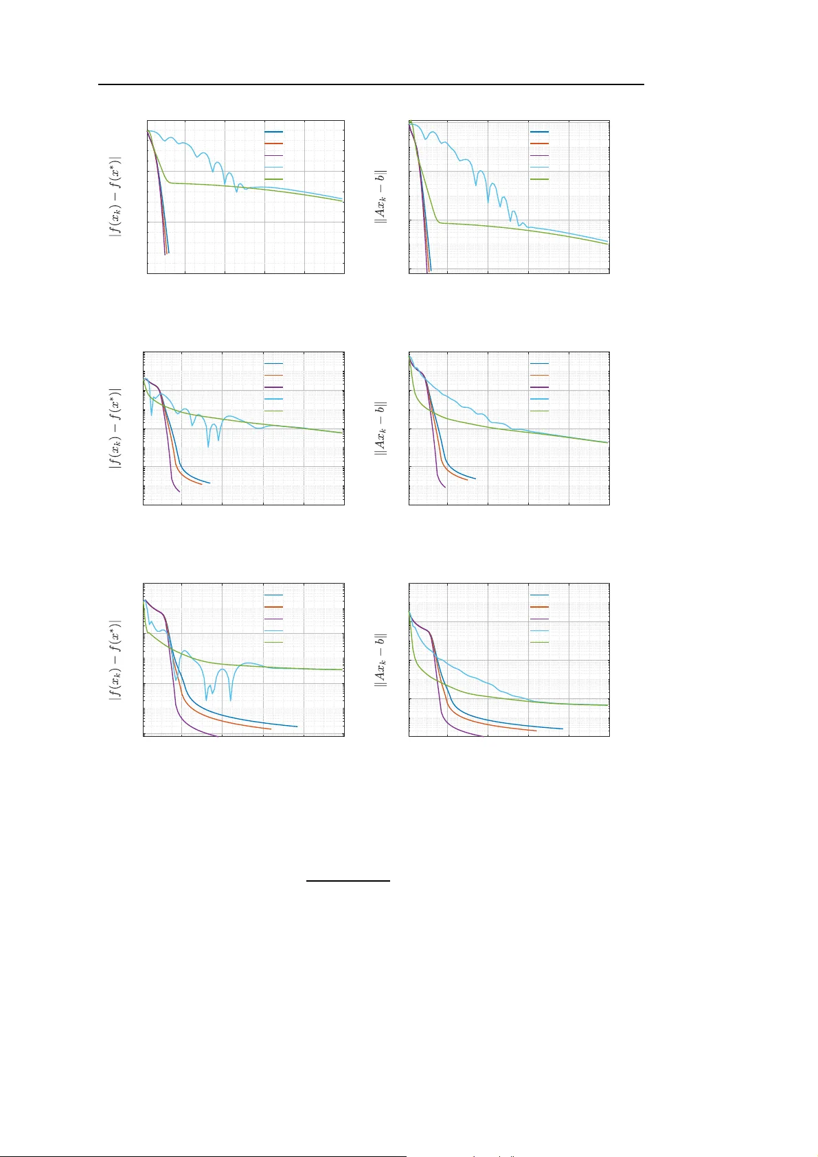
man uscript No. (will be inserted by the editor) Primal-dual dynamical systems with closed- lo op con trol for con v ex optimization in con tin u ous and discrete time Huan Zhang 1 · Xiangk ai Sun 2 · Sheng jie Li 1 · Kok La y T eo 3 Receiv ed: date / Accepted: date Abstract This pap er develops a primal-dua l dyna mical system wher e the co efficients are designed in c losed-lo op way for so lving a conv ex optimization pro blem with linear eq ua lit y constraints. W e firs t introduce a “ second-order primal” + “fir s t-order dual” c o n tinuous-time dynamical sys tem, in which b oth the time sca ling a nd Hessian-dr iv en damping are governed by a feedback control of the gra dien t for the Lagrangia n function. This system achiev es the fast c on vergence rates for the pr ima l-dual gap, the feasibility v iolation, and the ob jective residual along its tra jectory . Subsequently , by time discretization of this s y stem, we develop an acceler ated primal- dual a lgorithm with a gra dien t-defined ada ptiv e step size. W e also obtain conv ergence r ates for the primal-dual gap, the feasibility violation, and the ob jective residual. F urthermo re, we provide numerical results to demonstrate the pra ctical efficacy and super ior p erformance of the prop osed algorithm. Keyw ords Closed-lo op control · Prima l- dual a lgorithm · Conv ex optimization · Hes sian- driven damping Mathematics Sub ject Class ification (2000) 34D05 · 37N40 · 90 C25 Huan Zhang zhangh wxy@163.com Xiangk ai Sun sunxk@ctbu.edu.cn Shengjie Li ( B ) lisj@cqu.edu.cn Kok Lay T eo K.L.T eo@curtin.edu.au 1 College of Mathematics and Statistics, Chongqing Universit y , Chongqing 401331, China 2 Sc hool of Mathematics and Statistics, Chongqing T echn ology and Business Univ ersity , Chongqing 400067, China 3 Sc hool of Mathematica l Sciences, Sun wa y Universit y , Bandar Sunw ay , 47500 Selangor Darul Ehsan, Malaysia. 2 1 In tro duction 1.1 Problem description Let H and G b e real Hilber t spa ces equipp ed with inner pro duct h· , ·i and norm k · k . In this pap er, w e co nsider the convex optimization pro blem with linear equality c o nstrain ts of the form ( min x ∈H f ( x ) s.t. Ax = b, (1) where f : H → R is a differentiable conv ex function with L - Lipsc hitz contin uo us gr adien t for L > 0 , A : H → G is a contin uous linear op erator and b ∈ G . The optimization pro blem of the form ( 1 ) arises in ma n y applications acro ss fields such a s image recov ery , ma c hine learning, and netw or k optimization, see [ 1 – 4 ] and the references therein. The L a grangian function ass ociated with Pro blem ( 1 ) is defined as L ( x, λ ) := f ( x ) + h λ, Ax − b i , where λ ∈ G is the Lagra nge multiplier. A pair ( x ∗ , λ ∗ ) ∈ H × G is sa id to be a sa ddle po in t of the Lagra ngian function L iff L ( x ∗ , λ ) ≤ L ( x ∗ , λ ∗ ) ≤ L ( x, λ ∗ ) , ∀ ( x, λ ) ∈ H × G . In the sequel, the set of saddle points of L is denoted by S . The set of feasible p oin ts of Problem ( 1 ) is denoted by F := { x ∈ H | Ax = b } . F or any ( x, λ ) ∈ F × G , it holds that f ( x ) = L ( x, λ ). W e ass ume that S 6 = ∅ . Let ( x ∗ , λ ∗ ) ∈ S . Then, ( x ∗ , λ ∗ ) ∈ S ⇔ ( 0 = ∇ x L ( x ∗ , λ ∗ ) = ∇ f ( x ∗ ) + A ∗ λ ∗ , 0 = ∇ λ L ( x ∗ , λ ∗ ) = Ax ∗ − b, where A ∗ : G → H denotes the adjoint op erator of A . T o s olv e Pr oblem ( 1 ), in this pap er, we prop ose the following “ second-order primal” + “first-or der dual” dynamical system whose damping is a feedback control of the g radien t of the Lagra ng ian function:                    ¨ x ( t ) + 2[ ˙ τ ( t )] 2 − τ ( t ) ¨ τ ( t ) τ ( t ) ˙ τ ( t ) ˙ x ( t ) + [ ˙ τ ( t )] 2 τ ( t ) d dt ∇ x L ( x ( t ) , λ ( t )) + ˙ τ ( t )( ˙ τ ( t )+ ¨ τ ( t )) τ ( t ) ∇ x L ( x ( t ) , λ ( t )) = 0 , ˙ λ ( t ) − ˙ τ ( t ) ∇ λ L  x ( t ) + τ ( t ) ˙ τ ( t ) ˙ x ( t ) , λ ( t )  = 0 , τ ( t ) − 1 q q  t 0 + R t t 0 [ µ ( s )] 1 q ds  q = 0 , [ µ ( t )] p k∇ x L ( x ( t ) , λ ( t )) k p − 1 = 1 , (2) where q > 0, p ≥ 1, t ≥ t 0 > 0 and τ : [ t 0 , + ∞ ) → (0 , + ∞ ) is the time sc aling function which is non-decrea sing and c o n tinuously differentiable. W e obtain the fast conv ergence rates for the pr imal-dual gap, the feasibility violatio n, and the ob jective residual a lo ng the tra jectory generated by System ( 2 ). Subsequently , we prop ose an autonomous pr imal-dual a lgorithm by time discretization of System ( 2 ), and give some conv ergence a nalysis. 3 1.2 Motiv ation and related works Over the past decades, a series of studies hav e explored second-order dynamical systems in contin uous and discrete time for the unconstrained conv ex optimization problem min x ∈H f ( x ) . (3) Su et al. [ 5 ] prop osed the following se c o nd-order dyna mical system: ¨ x ( t ) + α t ˙ x ( t ) + ∇ f ( x ( t )) = 0 , (4) where α ≥ 3, and o bta ined the O  1 t 2  conv er gence rate o f the o b jective residual along the tra jectory generated by the system ( 4 ). The sy stem ( 4 ) has further b een studied in several pap ers, including [ 6 – 8 ]. They show ed that the o b jective re sidual co nverges at a r ate o f order o  1 t 2  for α > 3 , and the tra jectory weakly conv erges to the globa l minimizer of the ob jectiv e function. In order to improv e the co nvergence r ate, A ttouch et al. [ 9 ] pr o posed the system ( 4 ) with the time scaling: ¨ x ( t ) + α t ˙ x ( t ) + β ( t ) ∇ f ( x ( t )) = 0 , where α ≥ 1 a nd β : [ t 0 , + ∞ ) → (0 , + ∞ ) is the time s caling function which is non-decrea sing and contin uously differentiable. They o btained the O  1 t 2 β ( t )  conv er gence r ate of the ob- jective r esidual along the tra jectory gene r ated by this s ystem, and prop osed an iner tial proximal algor ithm by time discretization of this system. On the other hand, primal-dual dynamics metho ds were also attracted an increasing int erest by many res earc hers for solving the linear eq ualit y constrained conv ex o ptimiza - tion problem ( 1 ). Over the past few y ears , ther e hav e been a wide v ar ie t y of works devoted to “second-or der primal” + “second-o rder dual” contin uous-time dyna mical systems for solving Problem ( 1 ), see [ 10 – 13 ]. By time discretization of c on tinuous-time dyna mical sys- tems, new acceler ated primal-dual algo r ithms for so lving Pr oblem ( 1 ) hav e b een pro posed in [ 14 – 17 ]. Since the co mputational cos t of a primal- dua l metho d primarily a rises fr om the sub-problem inv olving the primal v aria ble, a nd a first-or der dynamica l sys tem is simpler and more trac table to solve than a second- o rder one, He et al. [ 18 ] prop osed the following “second-o rder pr imal” + “firs t-order dual” dynamical system for solving Pro blem ( 1 ): ( ¨ x ( t ) + γ ˙ x ( t ) + β ( t ) ∇ x L ( x ( t ) , λ ( t )) = 0 , ˙ λ ( t ) − β ( t ) ∇ λ L ( x ( t ) + δ ˙ x ( t ) , λ ( t )) = 0 , where γ > 0 and δ > 0. This system can b e viewed as an extension of Polyaks heavy ball with friction sy stem in [ 19 ]. Note that “ second-order primal” + “first-or der dual” dyna mical systems a nd discr ete ac celerated a lgorithms for solving Problem ( 1 ) ha ve b een studied in [ 20 – 23 ]. The pr esen t study is motiv ated by pr ior works in tw o domains: dynamical s ystems with Hessian-driven damping and those with closed-lo op control. W e now provide a comprehens iv e review of these resear ch areas. 4 1.2.1 Dynamic al systems with Hessian-driven damping It is w orth noting that the incorp oration of Hessian-dr iv en damping into the dynamical system has been a significant milestone in optimization and mechanics, as Hessian-driven damping can effectiv ely mitigate the oscillations. Building on this founda tio n, man y re- searchers use dynamical s ystems with Hessia n- driv en damping for solving the problem ( 3 ). Alv arez et al. [ 24 ] firs t prop osed the seco nd-order dynamical system with constant viscous damping and constant Hessian- driv en damping: ¨ x ( t ) + a ˙ x ( t ) + γ ∇ 2 f ( x ( t )) ˙ x ( t ) + b ∇ f ( x ( t )) = 0 , (5) where b = 1. They obtained some new conv ergence pro perties o f the so lution tra jector y generated by the system ( 5 ). Attouc h et a l. [ 25 ] established the system ( 5 ) with a = α t , and obta ined the O  1 t 2  conv er gence r a te of the ob jective res idua l for so lving the pr o blem ( 3 ). T o further accele r ate the conv ergence rate, A ttouch et al. [ 26 ] pro p osed the system ( 5 ) with a = α t and b = β ( t ), and o btained the O  1 t 2 β ( t )  conv er gence r ate for the ob jective residual. Mor eo ver, for leading to Nesterov-t y pe inertial alg orithms v ia standard implicit or explicit schemes, Alecs a et al. [ 2 7 ] prop osed the seco nd-order dynamical sys tem with implicit Hessian-driven damping: ¨ x ( t ) + α t ˙ x ( t ) + ∇ f  x ( t ) +  γ + β t  ˙ x ( t )  = 0 . They showed that inertial algor ithms, such as Nester ov’s alg orithm, ca n b e obtained v ia the natural explicit discre tiza tion from this dyna mical sys tem, and they also o bta ined the O  1 t 2  conv er gence rate of the ob jective residua l along the tra jectory generated by this sys tem. F o r more results on second or der dynamica l sy s tems with Hessian-driven damping for s o lving the problem ( 3 ), see [ 28 – 30 ] and the references therein. How ever, to the b est of our knowledge, it appea rs that there exist only few pap ers in the liter ature devoting to the study of prima l-dual dynamical systems with Hessian-driven damping in b oth contin uo us and discrete time for solving Pr oblem ( 1 ). Mor e precisely , He et al. [ 3 1 ] pro posed the following “seco nd- order primal” + “ first-order dual” dyna mical sy stem:    ¨ x ( t ) + α t ˙ x ( t ) + β ( t ) d dt ∇ x L ( x ( t ) , λ ( t )) + γ ( t ) ∇ x L ( x ( t ) , λ ( t )) = 0 , ˙ λ ( t ) − η ( t ) ∇ λ L  x ( t ) + t α − 1 ˙ x ( t ) , λ ( t )  = 0 , where t ≥ t 0 , α > 1 . They obtained the O  1 tη ( t )  conv er gence rate for the primal-dual g ap, feasibility v iolation and the o b jectiv e residual along the tra jectory gener ated by this system, and also obtained corr esponding conv ergence r ates for prop osed pr imal-dual algo rithm by time discretiza tio n of this system. Li et al. [ 32 ] prop osed a “se cond-order primal” +“second- order dual” dynamical system with implicit Hessian damping. They also established the fast conv er gence prop erties of the pr o posed dyna mica l s ystem under suitable conditions. F rom what was mentioned a bov e, we see that primal-dual dynamical systems with Hessia n-driv en damping for so lv ing conv ex optimization problems with linear equality constraints hav e so far r eceiv ed muc h less attent ion compared with other s. So, the firs t aim of this pap er is to inv estiga te primal-dual dy namical s ystems with Hessian-dr iv e n damping for solving Problem ( 1 ). 5 1.2.2 Dynamic al systems with close d-lo op c ontr ol The da mping co efficien ts of a clos e d-loop dynamica l system are directly governed b y its evolving tr a jectory , which c la ssifies the system as autono mo us. Unlike non- autonomous sys- tems, autono mo us ones are g enerally prefer red in prac tice b ecause they do not dep end on the time v ariable t . As far a s w e know, there are a few pap ers in the literature devoted to dynamical sy stems with closed-lo op co n tro l for the unconstrained conv ex optimization problem ( 3 ). Mo re prec isely , Attouc h et al. [ 33 ] prop osed an ine r tial dynamica l system with closed-lo op co ntrol: ¨ x ( t ) + γ ( t ) ˙ x ( t ) + ∇ f ( x ( t )) = 0 , (6) where t ≥ t 0 and γ ( t ) = k ˙ x ( t ) k p for several v alues of p ∈ R . They obtained the weak conv er gence of the tra jectories to o ptimal solutio ns . F or achieving c o n vergence r ate, Lin a nd Jordan [ 34 ] introduced a second-or der dynamical system with clos ed-loop control a s follows:          ¨ x ( t ) + 2[ ˙ τ ( t )] 2 − τ ( t ) ¨ τ ( t ) τ ( t ) ˙ τ ( t ) ˙ x ( t ) + [ ˙ τ ( t )] 2 τ ( t ) ∇ 2 f ( x ( t )) ˙ x ( t ) + ˙ τ ( t )( ˙ τ ( t )+ ¨ τ ( t )) τ ( t ) ∇ f ( x ( t )) = 0 , τ ( t ) − 1 4  c + R t 0 [ µ ( s )] 1 2 ds  2 = 0 , [ µ ( t )] p k∇ f ( x ( t )) k p − 1 = θ , (7) where c > 0 , θ ∈ (0 , 1), and p ≥ 1. They o btained the O  1 t 3 p +1 2  conv er gence rate for the o b jectiv e residua l along the tra jectory gener ated by the system ( 7 ), and provided tw o algorithmic fra mew o rks from time discretiza tion of this s ystem. Ma ier et al. [ 3 5 ] pro posed the system ( 6 ) with γ ( t ) := p E ( t ), wher e E ( t ) := f ( x ( t )) − f ( x ∗ ) + 1 2 k ˙ x ( t ) k 2 , and obtained the O  1 t 2 − δ  conv er gence rate for the ob jective res idual along the tra jectory genera ted by this system with δ > 0. By using time scaling and averaging tech nique, Attouc h et al. [ 36 ] developed autonomo us inertial dynamical s y stems which inv olve v anishing v iscous damping and implicit Hessian- driv en damping. They obtained the O  1 t 1+ q − 1 p  conv er gence rate for the o b jective res idua l a lo ng the tra jectory gener ated by this system with q > 0, p ≥ 1 and the weak conv ergence o f the tra jectories to optimal solutions. W e obser ve that there is no results dealing with primal-dual dynamical systems with closed-lo op con trol for solving Problem ( 1 ). So, the second aim of this pap er is to inv es- tigate primal-dual dynamical systems with closed-lo op control for solving Problem ( 1 ) in contin uous and discrete time. 1.3 Main contributions The contributions of this pap er can b e more sp ecifically stated as follows: • The contin uous level: W e prop ose a new “sec ond-order primal” + “firs t-order dual” dynamical sys tem ( 2 ) with time sca ling and Hes sian-driven da mping. The novelt y of Sy s tem ( 2 ) considered in this pap er when compare d with the system introduced in [ 18 ] is that Sys- tem ( 2 ) incorp orates Hessia n- driv en damping and all damping co efficien ts g o verned by the gradient of the Lagra ngian function with a feedback control. W e note that this is the fir st pap er for the in vestigation of primal- dual dy na mical systems with closed-lo op control for solving conv ex optimization problems with linear equality constra in ts. F urther, the conv er - gence rate of the ob jectiv e function residual obtained in this pap er ma tc hes that r eported in [ 34 ], which addresses System ( 2 ) for unconstra ined conv ex optimiza tio n problems. 6 • The di s crete lev el : W e develop an accelera ted autonomo us pr imal-dual a lgorithm, where the step size is adaptively defined ba sed on g r adien t of the ob jectiv e function for Problem ( 1 ). This makes our n umerical scheme muc h e a sier implementable than the n u- merical algo rithm prop osed in [ 34 ]. By appr opriately adjusting these pa rameters, we s how that this algo rithm pr opose d in this pap e r exhibits the O  1 k 3 p − 1 2 p  conv er gence r ate for the primal-dual gap, the feasibility viola tion, and the ob jective r esidual. Mo reov er, in numerical exp erimen ts, our alg orithm yields a significantly faster conv erg ence ra te and consistently achiev e s substantially higher a ccuracy than state-of-the-a rt metho ds. 1.4 Orga niz a tion The rest o f this paper is organize d as follows. In Section 2, we obtain fast co n vergence rates of the pr imal-dual gap, the feasibility violatio n, a nd the ob jectiv e residual along the tra jectories genera ted by System ( 2 ). In Section 3, we pro pose an acceler ated a utonomous primal-dual a lgorithm for so lving P roblem ( 1 ) a nd g iv e some co n vergence analy s is. In Section 4, w e present some numerical exp eriments to illustrate the obtained results. 2 The contin uous-tim e dynamical s ystem In this section, by using the Lyapunov analysis, we establish the fast co n vergence rates for the pr imal-dual gap, the feasibility violatio n, and the ob jective residual a lo ng the tra jectory generated by System ( 2 ) under mild as sumptions on the parameter s. T o b egin, we recall the following result which will play a n imp ortant ro le in the s equel. Lemma 2.1 [ 36 , Lemma 2 .2] Supp ose that ther e exist C 0 > 0 and b > a ≥ 0 such that Z t t 0 [ τ ( s )] a [ µ ( s )] − b ds ≤ C 0 < + ∞ , ∀ t ≥ t 0 , wher e τ is define d in terms of µ as in System ( 2 ) , n amely, τ ( t ) = 1 q q  t 0 + R t t 0 [ µ ( s )] 1 q ds  q . Then, ther e exists C 1 > 0 such that τ ( t ) ≥ C 1 ( t − t 0 ) qb +1 b − a , ∀ t ≥ t 0 . Now, we inv estig ate the conv er gence pr operties of System ( 2 ). Theorem 2. 1 L et ( x, λ ) : [ t 0 , + ∞ ) → H × G b e a solution of System ( 2 ) . Su pp ose t ha t q ≥ 1 and p ≥ 1 . Then, for any ( x ∗ , λ ∗ ) ∈ S , we have L ( x ( t ) , λ ∗ ) − L ( x ∗ , λ ∗ ) = O  1 t 2 qp − p +1 2  , a s t → + ∞ , k Ax ( t ) − b k = O  1 t 2 qp − p +1 2  , a s t → + ∞ , | f ( x ( t )) − f ( x ∗ ) | = O  1 t 2 qp − p +1 2  , as t → + ∞ , and Z + ∞ t 0 [ ˙ τ ( s )] 2 k∇ x L ( x ( s ) , λ ( s )) k 2 ds < + ∞ . F urt hermor e, ( x ( s ) , λ ( s )) is b ounde d over [ t 0 , t ] and the upp er b ound only dep ends on the initial c ondition. 7 Pr o of Clea rly , System ( 2 ) is equiv alent to the fo llo w ing sy s tem:                    ˙ v ( t ) + ˙ τ ( t ) ∇ x L ( x ( t ) , λ ( t )) = 0 , ˙ x ( t ) + ˙ τ ( t ) τ ( t ) ( x ( t ) − v ( t )) + [ ˙ τ ( t )] 2 τ ( t ) ∇ x L ( x ( t ) , λ ( t )) = 0 , ˙ λ ( t ) − ˙ τ ( t ) ∇ λ L  x ( t ) + τ ( t ) ˙ τ ( t ) ˙ x ( t ) , λ ( t )  = 0 , τ ( t ) − 1 q q  t 0 + R t t 0 [ µ ( s )] 1 q ds  q = 0 , [ µ ( t )] p k∇ x L ( x ( t ) , λ ( t )) k p − 1 = 1 . (8) F or any fixed ( x ∗ , λ ∗ ) ∈ S , we int ro duce the energy function E : [ t 0 , + ∞ ) → R which defined as E ( t ) := τ ( t ) ( L ( x ( t ) , λ ∗ ) − L ( x ∗ , λ ∗ )) + 1 2 k v ( t ) − x ∗ k 2 + 1 2 k λ ( t ) − λ ∗ k 2 . (9) Obviously , E ( t ) ≥ 0 for all t ≥ t 0 . Note that h ˙ v ( t ) , v ( t ) − x ∗ i = h ˙ v ( t ) , v ( t ) − x ( t ) i + h ˙ v ( t ) , x ( t ) − x ∗ i = h ˙ τ ( t ) ∇ x L ( x ( t ) , λ ( t )) , x ( t ) − v ( t ) i − h ˙ τ ( t ) ∇ x L ( x ( t ) , λ ( t )) , x ( t ) − x ∗ i . This together with ( 9 ) follows that ˙ E ( t ) = ˙ τ ( t ) [ L ( x ( t ) , λ ∗ ) − L ( x ∗ , λ ∗ )] + τ ( t ) h∇ x L ( x ( t ) , λ ∗ ) , ˙ x ( t ) i + h ˙ v ( t ) , v ( t ) − x ∗ i + h ˙ λ ( t ) , λ ( t ) − λ ∗ i = ˙ τ ( t ) [ L ( x ( t ) , λ ∗ ) − L ( x ∗ , λ ∗ ) − h∇ x L ( x ( t ) , λ ( t )) , x ( t ) − x ∗ i ] + τ ( t ) h∇ x L ( x ( t ) , λ ∗ ) , ˙ x ( t ) i + ˙ τ ( t ) h∇ x L ( x ( t ) , λ ( t )) , x ( t ) − v ( t ) i + h ˙ λ ( t ) , λ ( t ) − λ ∗ i = ˙ τ ( t ) [ L ( x ( t ) , λ ∗ ) − L ( x ∗ , λ ∗ ) − h∇ x L ( x ( t ) , λ ∗ ) , x ( t ) − x ∗ i ] − ˙ τ ( t ) h λ ( t ) − λ ∗ , Ax ( t ) − b i + τ ( t ) h∇ x L ( x ( t ) , λ ( t )) , ˙ x ( t ) i − τ ( t ) h λ ( t ) − λ ∗ , A ˙ x ( t ) i + ˙ τ ( t ) h∇ x L ( x ( t ) , λ ( t )) , x ( t ) − v ( t ) i + h ˙ λ ( t ) , λ ( t ) − λ ∗ i = ˙ τ ( t ) [ L ( x ( t ) , λ ∗ ) − L ( x ∗ , λ ∗ ) − h∇ x L ( x ( t ) , λ ∗ ) , x ( t ) − x ∗ i ] + h∇ x L ( x ( t ) , λ ( t )) , τ ( t ) ˙ x ( t ) + ˙ τ ( t )( x ( t ) − v ( t )) i , where the third equality ho lds due to ∇ x L ( x ( t ) , λ ( t )) = ∇ x L ( x ( t ) , λ ∗ ) + A ∗ ( λ ( t ) − λ ∗ ) and the last equality holds due to the third equatio n of ( 8 ) and ∇ λ L  x ( t ) + τ ( t ) ˙ τ ( t ) ˙ x ( t ) , λ ( t )  = A  x ( t ) + τ ( t ) ˙ τ ( t ) ˙ x ( t )  − b. By using the conv exity o f L ( · , λ ∗ ), we hav e L ( x ( t ) , λ ∗ ) − L ( x ∗ , λ ∗ ) − h∇ x L ( x ( t ) , λ ∗ ) , x ( t ) − x ∗ i ≤ 0 . F rom the second equation of the system ( 8 ), we hav e h∇ x L ( x ( t ) , λ ( t )) , τ ( t ) ˙ x ( t ) + ˙ τ ( t )( x ( t ) − v ( t )) i = − [ ˙ τ ( t )] 2 k∇ x L ( x ( t ) , λ ( t )) k 2 . Thu s, ˙ E ( t ) ≤ − [ ˙ τ ( t )] 2 k∇ x L ( x ( t ) , λ ( t )) k 2 ≤ 0 . (10) This implies E ( t ) ≤ E ( t 0 ) for all t ≥ t 0 . By the definition of E ( t ), we obtain that L ( x ( t ) , λ ∗ ) − L ( x ∗ , λ ∗ ) ≤ E ( t 0 ) τ ( t ) = O  1 τ ( t )  , as t → + ∞ , 8 and λ ( t ) is b ounded on [ t 0 , + ∞ ) and the upp er b ound only dep ends o n the initial condition. F rom the third equation of the system ( 8 ), we hav e λ ( t ) − λ ( t 0 ) = Z t t 0 ˙ λ ( s ) ds = Z t t 0 ˙ τ ( s )  Ax ( s ) − b + τ ( s ) ˙ τ ( s ) A ˙ x ( t )  ds = τ ( t )( Ax ( t ) − b ) − τ ( t 0 )( Ax ( t 0 ) − b ) . Then, k τ ( t )( Ax ( t ) − b ) k < + ∞ , which means that k Ax ( t ) − b k ≤ O  1 τ ( t )  , as t → + ∞ . F rom the definition of L , we hav e | f ( x ( t )) − f ( x ∗ ) | ≤ L ( x ( t ) , λ ∗ ) − L ( x ∗ , λ ∗ ) + k λ ∗ kk Ax ( t ) − b k ≤ O  1 τ ( t )  , as t → + ∞ . On the other hand, we deduce from ( 10 ) that ˙ E ( t ) + [ ˙ τ ( t )] 2 k∇ x L ( x ( t ) , λ ( t )) k 2 ≤ 0 . Then, E ( t ) + Z t t 0 [ ˙ τ ( s )] 2 k∇ x L ( x ( s ) , λ ( s )) k 2 ds ≤ E ( t 0 ) . (11) It follows that Z + ∞ t 0 [ ˙ τ ( s )] 2 k∇ x L ( x ( s ) , λ ( s )) k 2 ds ≤ E ( t 0 ) < + ∞ . (12) F rom the fourth equation of the system ( 8 ), w e hav e ˙ τ ( t ) = [ τ ( t )] q − 1 q [ µ ( t )] 1 q . (13) This together with the last equation of the system ( 8 ) yields [ ˙ τ ( t )] 2 k∇ x L ( x ( t ) , λ ( t )) k 2 = [ τ ( t )] 2 q − 2 q [ µ ( t )] 2 q − 2 p p − 1 . (14) T ogether with ( 12 ), ( 14 ) and Lemma 2.1 , there exists C 1 > 0 such that τ ( t ) ≥ C 1 ( t − t 0 ) 2 qp − p +1 2 . (15) Thu s, L ( x ( t ) , λ ∗ ) − L ( x ∗ , λ ∗ ) = O  1 t 2 qp − p +1 2  , as t → + ∞ , k Ax ( t ) − b k = O  1 t 2 qp − p +1 2  , as t → + ∞ , and | f ( x ( t )) − f ( x ∗ ) | = O  1 t 2 qp − p +1 2  , as t → + ∞ . Now, we only need to show that τ ( s ) is b ounded ov er [ t 0 , t ] a nd the upp er b ound only depe nds o n the initial condition. In fact, by us ing the definition of E ( t ) and E ( t ) ≤ E ( t 0 ), we hav e 1 2 k v ( t ) − x ∗ k 2 ≤ E ( t 0 ) . 9 This follows that v ( t ) is b ounded ov er [ t 0 , + ∞ ) and the upp er b ound only dep e nds on the initial condition. Note that τ ( t )( x ( t ) − x ∗ ) − τ ( t 0 )( x ( t 0 ) − x ∗ ) = Z t t 0 [ ˙ τ ( s )( x ( s ) − x ∗ ) + τ ( s ) ˙ x ( s )] ds. Then, k τ ( t )( x ( t ) − x ∗ ) k ≤ τ ( t 0 ) k x ( t 0 ) − x ∗ k + Z t t 0 k ˙ τ ( s )( x ( s ) − x ∗ ) + τ ( s ) ˙ x ( s ) k ds ≤ τ ( t 0 ) k x ( t 0 ) − x ∗ k + Z t t 0 k ˙ τ ( s )( v ( s ) − x ∗ ) k ds + Z t t 0 [ ˙ τ ( s )] 2 k∇ x L ( x ( s ) , λ ( s )) k ds, (16) where the last inequality holds due to the second eq ua tion of system ( 8 ). F ro m ( 1 3 ) and the last equation of system ( 8 ), we hav e [ ˙ τ ( t )] 2 k∇ x L ( x ( t ) , λ ( t )) k = [ τ ( t )] 2 q − 2 q k∇ x L ( x ( t ) , λ ( t )) k qp +2 − 2 p qp . (17) Combined with ( 16 ), ( 17 ), k v ( t ) − x ∗ k ≤ p 2 E ( t 0 ) a nd the fact tha t τ ( t ) is monoto nically increasing, we hav e k x ( t ) − x ∗ k ≤ τ ( t 0 ) k x ( t 0 ) − x ∗ k + p 2 E ( t 0 )( τ ( t ) − τ ( t 0 )) τ ( t ) + 1 τ ( t ) Z t t 0    [ τ ( s )] 2 q − 2 q ∇ x L ( x ( s ) , λ ( s )) qp +2 − 2 p qp    ds ≤k x ( t 0 ) − x ∗ k + p 2 E ( t 0 ) + 1 τ ( t ) Z t t 0 [ τ ( s )] 2 q − 2 q k∇ x L ( x ( s ) , λ ( s )) k qp +2 − 2 p qp ds. (18) Note that 1 τ ( t ) Z t t 0 [ τ ( s )] 2 q − 2 q k∇ x L ( x ( s ) , λ ( s )) k qp +2 − 2 p qp ds = 1 τ ( t ) Z t t 0 [ τ ( s )] qp − 2 p 2 qp +2 − 2 p [ τ ( s )] qp 2 qp +2 − 2 p  [ τ ( s )] 2 q − 2 q k∇ x L ( x ( s ) , λ ( s )) k 2 qp +2 − 2 p qp  qp +2 − 2 p 2 qp +2 − 2 p ds. (19) Now, we analyze ( 19 ) in terms of the following tw o ca ses. Case I : 1 ≤ q < 2 a nd 1 ≤ p ≤ 2 2 − q . In this case, from H¨ older inequality and the fa c t that τ ( t ) is monotonically increas ing , ther e exists C 2 > 0 such that 1 τ ( t ) Z t t 0 [ τ ( s )] qp − 2 p 2 qp +2 − 2 p [ τ ( s )] qp 2 qp +2 − 2 p  [ τ ( s )] 2 q − 2 q k∇ x L ( x ( s ) , λ ( s )) k 2 qp +2 − 2 p qp  qp +2 − 2 p 2 qp +2 − 2 p ds ≤ [ τ ( t 0 )] qp − 2 p 2 qp +2 − 2 p 1 τ ( t )  Z t t 0 τ ( s ) ds  qp 2 qp +2 − 2 p  Z t t 0 [ τ ( s )] 2 q − 2 q k∇ x L ( x ( s ) , λ ( s )) k 2 qp +2 − 2 p qp ds  qp +2 − 2 p 2 qp +2 − 2 p ≤ C 2 [ τ ( t 0 )] qp − 2 p 2 qp +2 − 2 p [ τ ( t )] − qp +2 − 2 p 2 qp +2 − 2 p  Z t t 0 [ τ ( s )] 2 q − 2 q k∇ x L ( x ( s ) , λ ( s )) k 2 qp +2 − 2 p qp ds  qp +2 − 2 p 2 qp +2 − 2 p ≤ C 2 [ τ ( t 0 )] − 2 2 qp +2 − 2 p  Z t t 0 [ τ ( s )] 2 q − 2 q k∇ x L ( x ( s ) , λ ( s )) k 2 qp +2 − 2 p qp ds  qp +2 − 2 p 2 qp +2 − 2 p . (20) F rom ( 12 ) and ( 17 ), we hav e Z t t 0 [ τ ( s )] 2 q − 2 q k∇ x L ( x ( s ) , λ ( s )) k 2 qp +2 − 2 p qp ds = Z t t 0 [ ˙ τ ( s )] 2 k∇ x L ( x ( s ) , λ ( s )) k 2 ds ≤ E ( t 0 ) . (21) 10 T ogether with ( 18 ), ( 19 ), ( 20 ) and ( 21 ), we get k x ( t ) − x ∗ k ≤ k x ( t 0 ) − x ∗ k + p 2 E ( t 0 ) + C 2 [ τ ( t 0 )] − 2 2 qp +2 − 2 p [ E ( t 0 )] qp +2 − 2 p 2 qp +2 − 2 p . Case I I : q ≥ 2 and p ≥ 1 . In this case, fro m H¨ older inequality and the fact that τ ( t ) is monotonically increasing, there exists C 3 > 0 such that 1 τ ( t ) Z t t 0 [ τ ( s )] qp − 2 p 2 qp +2 − 2 p [ τ ( s )] qp 2 qp +2 − 2 p  [ τ ( s )] 2 q − 2 q k∇ x L ( x ( s ) , λ ( s )) k 2 qp +2 − 2 p qp  qp +2 − 2 p 2 qp +2 − 2 p ds ≤ [ τ ( t )] − qp − 2 2 qp +2 − 2 p  Z t t 0 τ ( s ) ds  qp 2 qp +2 − 2 p  Z t t 0 [ τ ( s )] 2 q − 2 q k∇ x L ( x ( s ) , λ ( s )) k 2 qp +2 − 2 p qp ds  qp +2 − 2 p 2 qp +2 − 2 p ≤ C 3 [ τ ( t )] − 2 2 qp +2 − 2 p  Z t t 0 [ τ ( s )] 2 q − 2 q k∇ x L ( x ( s ) , λ ( s )) k 2 qp +2 − 2 p qp ds  qp +2 − 2 p 2 qp +2 − 2 p ≤ C 3 [ τ ( t 0 )] − 2 2 qp +2 − 2 p  Z t t 0 [ τ ( s )] 2 q − 2 q k∇ x L ( x ( s ) , λ ( s )) k 2 qp +2 − 2 p qp ds  qp +2 − 2 p 2 qp +2 − 2 p . This together with ( 18 ), ( 19 ) and ( 21 ) gives k x ( t ) − x ∗ k ≤ k x ( t 0 ) − x ∗ k + p 2 E ( t 0 ) + C 3 [ τ ( t 0 )] − 2 2 qp +2 − 2 p [ E ( t 0 )] qp +2 − 2 p 2 qp +2 − 2 p . F rom b oth cases, it follows that x ( s ) is b ounded over [ t 0 , t ] and the upper b ound only depe nds on the initial condition. ⊓ ⊔ R emark 2.1 Note tha t Attouc h et al. [ 36 ] in tro duced a sec o nd-order dynamical system via closed-lo op c o n tr ol of the gradient for solving the problem ( 3 ). In [ 36 , Theor em 3.5 ], they ob- tained the o  ln( t ) t pq  conv er gence rate for the o b jective residual alo ng the tr a jectory g enerated by the system. Theorem 2.1 extends [ 36 , Theor em 3 .5] from the unco nstrained optimization problem to Problem ( 3 ), and achiev es a faster conv e rgence rate for the ob jectiv e r esidual. Now, let us consider sp ecial cases o f Sys tem ( 2 ). In the sp ecial ca se when q = 1, System ( 2 ) collapses to                    ¨ x ( t ) + 2[ ˙ τ ( t )] 2 − τ ( t ) ¨ τ ( t ) τ ( t ) ˙ τ ( t ) ˙ x ( t ) + [ ˙ τ ( t )] 2 τ ( t ) d dt ∇ x L ( x ( t ) , λ ( t )) + ˙ τ ( t )( ˙ τ ( t )+ ¨ τ ( t )) τ ( t ) ∇ x L ( x ( t ) , λ ( t )) = 0 , ˙ λ ( t ) − ˙ τ ( t ) ∇ λ L  x ( t ) + τ ( t ) ˙ τ ( t ) ˙ x ( t ) , λ ( t )  = 0 , ˙ τ ( t ) = µ ( t ) , [ µ ( t )] p k∇ x L ( x ( t ) , λ ( t )) k p − 1 = 1 . (22) Corollary 2.1 L et ( x, λ ) : [ t 0 , + ∞ ) → H × G b e a solution of the system ( 22 ) . Supp ose that p ≥ 1 . Then, for any ( x ∗ , λ ∗ ) ∈ S , we have L ( x ( t ) , λ ∗ ) − L ( x ∗ , λ ∗ ) = O  1 t p +1 2  , as t → + ∞ , k Ax ( t ) − b k = O  1 t p +1 2  , as t → + ∞ , | f ( x ( t )) − f ( x ∗ ) | = O  1 t p +1 2  , a s t → + ∞ , and Z + ∞ t 0 [ ˙ τ ( s )] 2 k∇ x L ( x ( s ) , λ ( s )) k 2 ds < + ∞ . F urt hermor e, ( x ( s ) , λ ( s )) is b ounde d over [ t 0 , t ] and the upp er b ound only dep ends on the initial c ondition. 11 In the s pecial cas e whe n q = 2, System ( 2 ) co llapses to the following system:                    ¨ x ( t ) + 2[ ˙ τ ( t )] 2 − τ ( t ) ¨ τ ( t ) τ ( t ) ˙ τ ( t ) ˙ x ( t ) + [ ˙ τ ( t )] 2 τ ( t ) d dt ∇ x L ( x ( t ) , λ ( t )) + ˙ τ ( t )( ˙ τ ( t )+ ¨ τ ( t )) τ ( t ) ∇ x L ( x ( t ) , λ ( t )) = 0 , ˙ λ ( t ) − ˙ τ ( t ) ∇ λ L  x ( t ) + τ ( t ) ˙ τ ( t ) ˙ x ( t ) , λ ( t )  = 0 , τ ( t ) − 1 4  t 0 + R t t 0 [ µ ( s )] 1 2 ds  2 = 0 , [ µ ( t )] p k∇ x L ( x ( t ) , λ ( t )) k p − 1 = 1 . (23) Corollary 2.2 L et ( x, λ ) : [ t 0 , + ∞ ) → H × G b e a solution of the system ( 23 ) . Supp ose that p ≥ 1 . Then, for any ( x ∗ , λ ∗ ) ∈ S , we have L ( x ( t ) , λ ∗ ) − L ( x ∗ , λ ∗ ) = O  1 t 3 p +1 2  , as t → + ∞ , k Ax ( t ) − b k = O  1 t 3 p +1 2  , a s t → + ∞ , | f ( x ( t )) − f ( x ∗ ) | = O  1 t 3 p +1 2  , as t → + ∞ , and Z + ∞ t 0 [ ˙ τ ( s )] 2 k∇ x L ( x ( s ) , λ ( s )) k 2 ds < + ∞ . F urt hermor e, ( x ( s ) , λ ( s )) is b ounde d over [ t 0 , t ] and the upp er b ound only dep ends on the initial c ondition. R emark 2.2 Note that Lin and Michael [ 34 ] int ro duced the second-order dynamical system with closed-lo op control ( 7 ). In [ 34 , Theorem 3], they obtained f ( x ( t )) − f ( x ∗ ) = O  1 t 3 p +1 2  , as t → + ∞ . Therefore, Coro llary 2.2 extends [ 34 , Theorem 3] from the unco nstrained optimization pr ob- lem to Problem ( 3 ). In the sp e cial case for Sys tem ( 2 ) when p = q = 1 . This implies that µ ( t ) = 1 and τ ( t ) = t . System ( 2 ) collapse s to the following op en-lo op sys tem: ( ¨ x ( t ) + 2 t ˙ x ( t ) + 1 t d dt ∇ x L ( x ( t ) , λ ( t )) + 1 t ∇ x L ( x ( t ) , λ ( t )) = 0 , ˙ λ ( t ) − ∇ λ L ( x ( t ) + t ˙ x ( t ) , λ ( t )) = 0 . (24) Corollary 2.3 L et ( x, λ ) : [ t 0 , + ∞ ) → H × G b e a solution of System ( 24 ) . Then, for any ( x ∗ , λ ∗ ) ∈ S , we have L ( x ( t ) , λ ∗ ) − L ( x ∗ , λ ∗ ) = O  1 t  , a s t → + ∞ , k Ax ( t ) − b k = O  1 t  , as t → + ∞ , | f ( x ( t )) − f ( x ∗ ) | = O  1 t  , a s t → + ∞ , and Z + ∞ t 0 k∇ x L ( x ( s ) , λ ( s )) k 2 ds < + ∞ . F urt hermor e, ( x ( s ) , λ ( s )) is b ounde d over [ t 0 , t ] and the upp er b ound only dep ends on the initial c ondition. 12 R emark 2.3 The system ( 2 4 ) can b e a s a s pecial case o f the system prop osed in [ 31 ]. Clea rly , the para meters of the sys tem ( 24 ) satisfy the Assumption 2.1 in [ 3 1 ]. Th us, by Theor em 2.3 in [ 31 ], we hav e L ( x ( t ) , λ ∗ ) − L ( x ∗ , λ ∗ ) = O  1 t  , as t → + ∞ , k Ax ( t ) − b k = O  1 t  , as t → + ∞ , and | f ( x ( t )) − f ( x ∗ ) | = O  1 t  , as t → + ∞ , which is compatible with the results in Corolla ry 2.3 . 3 The dis crete accelerated autonom ous primal-dual algorithm In this section, w e prop ose an accelera ted a utonomous primal- dua l algo rithm with adaptive step s ize defined via gra dien t and a nalyze the conv ergence pr operties of this algorithm. F or simplicity , w e restrict our discussion to the case where q = 1, which gives ˙ τ ( t ) = µ ( t ). Obviously , the system ( 22 ) can be r eform ulated as:                    y ( t ) = x ( t ) + τ ( t ) ˙ τ ( t ) ˙ x ( t ) , ˙ y ( t ) = − ˙ τ ( t ) d dt ∇ x L ( x ( t ) , λ ( t )) − ( ˙ τ ( t ) + ¨ τ ( t )) ∇ x L ( x ( t ) , λ ( t )) , ˙ λ ( t ) = ˙ τ ( t ) ( Ay ( t ) − b ) , ˙ τ ( t ) = µ ( t ) , [ µ ( t )] p k∇ x L ( x ( t ) , λ ( t )) k p − 1 = 1 . (25) F or the system ( 25 ), we consider the time s tep size 1 and set y ( k ) ≈ y k , x ( k ) ≈ x k , τ ( k ) ≈ τ k , ˙ τ ( k ) ≈ γ k , λ ( k ) ≈ λ k , and µ ( k ) ≈ µ k . Ev aluating the terms d dt ∇ x L ( x ( t ) , λ ( t )) and ¨ τ ( t ) as the time deriv ative of ∇ x L ( x ( t ) , λ ( t )) and ˙ τ ( t ), resp ectiv ely . Now, by the time discretiza tion of the system ( 25 ), we hav e                              y k = x k + τ k γ k ( x k − x k − 1 ) , y k +1 − y k = − γ k [ ∇ f ( x k +1 ) + A ∗ λ k +1 − ( ∇ f ( x k ) + A ∗ λ k )] − ( γ k +1 + γ k +1 − γ k ) ( ∇ f ( x k +1 ) + A ∗ λ k +1 ) , λ k +1 − λ k = γ k +1 ( Ay k +1 − b ) , τ k +1 = γ k + τ k , γ k +1 = µ k , µ p k k∇ x L ( x k , λ k ) k p − 1 = 1 . (26) Substituting the first equation and the third eq ua tion into the second equatio n in ( 26 ), we hav e ∇ f ( x k +1 ) + γ k +1 + τ k +1 2 γ 2 k +1 ( x k +1 − ¯ x k ) + ( γ k +1 + τ k +1 ) A ∗ ( Ax k +1 − σ k +1 ) = 0 , where ¯ x k := x k + γ k +1 γ k +1 + τ k +1  τ k γ k ( x k − x k − 1 ) + γ k ( ∇ f ( x k ) + A ∗ λ k )  , 13 and σ k +1 := 1 γ k +1 + τ k +1 ( τ k +1 Ax k + γ k +1 b − λ k ) . This implies that x k +1 = arg min x ∈H  f ( x ) + γ k +1 + τ k +1 4 γ 2 k +1 k x − ¯ x k k 2 + γ k +1 + τ k +1 2 k Ax − σ k +1 k 2  . Based on the ab ov e analysis, we are now in the p osition to introduce the following accele r ated autonomous primal-dual algor ithm for so lving Pr oblem ( 1 ). Algorithm 1 Acceler ated autonomo us primal-dual algor ithm (AAPDA) Initializa tion: Cho ose x 0 = x 1 ∈ H and λ 1 ∈ G . Let p > 1, τ 1 = 0 and γ 1 ≥ 1. for k = 1 , 2 , . . . do if ∇ x L ( x k , λ k ) = 0 , then stop else Step 1: Compute µ k = k∇ x L ( x k , λ k ) k − p − 1 p , (27) γ k +1 = µ k , (28) τ k +1 = γ k + τ k , (29) ¯ x k := x k + γ k +1 γ k +1 + τ k +1  τ k γ k ( x k − x k − 1 ) + γ k ( ∇ f ( x k ) + A ∗ λ k )  , (30) σ k +1 := 1 γ k +1 + τ k +1 ( τ k +1 Ax k + γ k +1 b − λ k ) . (31) Step 2: Up date the primal v ari able x k +1 = arg min x ∈H ( f ( x ) + γ k +1 + τ k +1 4 γ 2 k +1 k x − ¯ x k k 2 + γ k +1 + τ k +1 2 k Ax − σ k +1 k 2 ) . (32) Step 3: Compute y k +1 = x k +1 + τ k +1 γ k +1 ( x k +1 − x k ) , (33) and up dat e the dual v ariable λ k +1 = λ k + γ k +1 ( Ay k +1 − b ) . (34) end if end for In o rder to ana ly ze the conv ergence r ates of AAPDA, we need the following re sult. Lemma 3.1 [ 36 , Lemma 4.2] L et { µ k } k ≥ 0 b e a p ositive se quenc e and { τ k } k ≥ 1 such that τ 1 = 0 and τ k = P k − 2 i =0 µ i for al l k ≥ 2 . Su pp ose that ther e exist C 4 > 0 and a, b, c ≥ 0 such that b + c > a and X k ≥ 0 τ a k µ − b k µ − c k +1 ≤ C 4 < + ∞ . Then, ther e exists C 5 > 0 such that for every k ≥ 2 , it holds τ k +1 ≥ C 5 k b + c +1 b + c − a . The fo llo wing equality will be use d in the sequel: 1 2 k x 1 k 2 − 1 2 k x 2 k 2 = h x 1 , x 1 − x 2 i − 1 2 k x 1 − x 2 k 2 , ∀ x 1 , x 2 ∈ H . (35) Now, we prove the conv e r gence ra tes of the pr imal-dual gap, the feasibility viola tion, and the ob jective r esidual gener ated by AAPDA . 14 Theorem 3. 1 L et { ( x k , λ k ) } k ≥ 0 b e the se quenc e gener ate d by AAPDA . Su pp ose that { µ k } k ≥ 0 is a non-de cr e asing se qu enc e satisfying µ k ≥ 1 for al l k ≥ 0 . Also, let { τ k } k ≥ 1 b e a se quenc e such that τ 1 = 0 and τ k = P k − 2 i =0 µ i for al l k ≥ 2 . Then, for any ( x ∗ , λ ∗ ) ∈ S , we have L ( x k , λ ∗ ) − L ( x ∗ , λ ∗ ) = O  1 k 3 p − 1 2 p  , as k → + ∞ , k Ax k − b k = O  1 k 3 p − 1 2 p  , as k → + ∞ , | f ( x k ) − f ( x ∗ ) | = O  1 k 3 p − 1 2 p  , as k → + ∞ , and + ∞ X k =0 γ 2 k +1 k∇ x L ( x k +1 , λ k +1 ) k 2 < + ∞ . Pr o of F o r ( x ∗ , λ ∗ ) ∈ S , we introduce the energy sequenc e which defined as E k := τ k +1 ( L ( x k , λ ∗ ) − L ( x ∗ , λ ∗ )) + 1 2 k u k k 2 + 1 2 k λ k − λ ∗ k 2 , where u k := y k − x ∗ + γ k ∇ x L ( x k , λ k ). Clearly , fr om ( 30 ), ( 31 ), ( 32 ), ( 33 ) and ( 34 ) (se e also the se c ond equa tio n o f s ystem ( 26 )), it is easy to show that y k +1 − y k = γ k ∇ x L ( x k , λ k ) − 2 γ k +1 ∇ x L ( x k +1 , λ k +1 ) . Then, u k +1 − u k = y k +1 − y k + γ k +1 ∇ x L ( x k +1 , λ k +1 ) − γ k ∇ x L ( x k , λ k ) = − γ k +1 ∇ x L ( x k +1 , λ k +1 ) . This together with ( 35 ) and ∇ x L ( x k +1 , λ k +1 ) = ∇ x L ( x k +1 , λ ∗ ) + A ∗ ( λ k +1 − λ ∗ ) gives 1 2 k u k +1 k 2 − 1 2 k u k k 2 = h u k +1 − u k , u k +1 i − 1 2 k u k +1 − u k k 2 ≤ − γ k +1 h∇ x L ( x k +1 , λ k +1 ) , y k +1 − x ∗ i − γ 2 k +1 k∇ x L ( x k +1 , λ k +1 ) k 2 = − γ k +1 h∇ x L ( x k +1 , λ ∗ ) , y k +1 − x ∗ i − γ k +1 h A ∗ ( λ k +1 − λ ∗ ) , y k +1 − x ∗ i − γ 2 k +1 k∇ x L ( x k +1 , λ k +1 ) k 2 . (36) F rom ( 33 ) and the conv exity o f L ( · , λ ∗ ), we hav e − γ k +1 h∇ x L ( x k +1 , λ ∗ ) , y k +1 − x ∗ i = − γ k +1 h∇ x L ( x k +1 , λ ∗ ) , x k +1 − x ∗ i − τ k +1 h∇ x L ( x k +1 , λ ∗ ) , x k +1 − x k i ≤ − γ k +1 ( L ( x k +1 , λ ∗ ) − L ( x ∗ , λ ∗ )) − τ k +1 ( L ( x k +1 , λ ∗ ) − L ( x k , λ ∗ )) = − ( γ k +1 + τ k +1 )( L ( x k +1 , λ ∗ ) − L ( x ∗ , λ ∗ )) + τ k +1 ( L ( x k , λ ∗ ) − L ( x ∗ , λ ∗ )) . (37) On the other hand, it follows from ( 34 ) and ( 35 ) that − γ k +1 h A ∗ ( λ k +1 − λ ∗ ) , y k +1 − x ∗ i = − γ k +1 h λ k +1 − λ ∗ , A y k +1 − b i = −h λ k +1 − λ ∗ , λ k +1 − λ k i = − 1 2  k λ k +1 − λ ∗ k 2 − k λ k − λ ∗ k 2 + k λ k +1 − λ k k 2  . (38) 15 T ogether with ( 36 )–( 38 ), we hav e E k +1 − E k = τ k +2 ( L ( x k +1 , λ ∗ ) − L ( x ∗ , λ ∗ )) − τ k +1 ( L ( x k , λ ∗ ) − L ( x ∗ , λ ∗ )) + 1 2 k u k +1 k 2 − 1 2 k u k k 2 + 1 2 k λ k +1 − λ ∗ k 2 − 1 2 k λ k − λ ∗ k 2 ≤ ( τ k +2 − τ k +1 − γ k +1 ) ( L ( x k +1 , λ ∗ ) − L ( x ∗ , λ ∗ )) − γ 2 k +1 k∇ x L ( x k +1 , λ k +1 ) k 2 − 1 2 k λ k +1 − λ k k 2 ≤ 0 , (39) where the last inequality holds due to ( 29 ). Thus, the sequence { E k } k ≥ 0 is non- inc r easing. This implies that L ( x k , λ ∗ ) − L ( x ∗ , λ ∗ ) = O  1 τ k +1  , as k → + ∞ , (40) and { λ k } k ≥ 0 is b ounded. F or notation simplicity , denote a sequence { g k } k ≥ 0 by g k := τ k +1 ( Ax k − b ) . It follows from ( 29 ), ( 33 ) and ( 34 ) that λ k +1 − λ 0 = k X j =0 ( λ j +1 − λ j ) = k X j =0 γ j +1 ( Ay j +1 − b ) = k X j =0 [( γ j +1 + τ j +1 )( Ax j +1 − b ) − τ j +1 ( Ax j − b )] = k X j =0 ( g j +1 − g j ) = g k +1 − g 0 . This together with the bo undedness o f { λ k } k ≥ 0 follows that sup k ≥ 0 k g k k < + ∞ . Then, k Ax k − b k ≤ O  1 τ k +1  , as k → + ∞ . (41) Combining ( 40 ), ( 41 ) and the definition of L , we hav e | f ( x k ) − f ( x ∗ ) | ≤ L ( x k , λ ∗ ) − L ( x ∗ , λ ∗ ) + k λ ∗ kk Ax k − b k ≤ O  1 τ k +1  , as k → + ∞ . (42 ) Summing ( 39 ) ov er k = 0 , . . . , N , we obtain N X k =0 γ 2 k +1 k∇ x L ( x k +1 , λ k +1 ) k 2 ≤ E 0 − E N ≤ E 0 . Letting N → + ∞ in the ab o ve inequality , we obtain + ∞ X k =0 γ 2 k +1 k∇ x L ( x k +1 , λ k +1 ) k 2 < + ∞ . 16 This together with ( 27 ) and ( 28 ) gives + ∞ X k =0 µ 2 k µ − 2 p p − 1 k +1 < + ∞ . F rom µ k ≥ 1 for all k ≥ 0, we hav e + ∞ X k =0 µ − 2 p p − 1 k +1 ≤ + ∞ X k =0 µ 2 k µ − 2 p p − 1 k +1 < + ∞ . Then, by using Lemma 3.1 , there exists C 3 > 0 such that τ k +1 ≥ C 3 k 3 p − 1 2 p . This together with ( 40 ), ( 41 ) and ( 42 ) follows that L ( x k , λ ∗ ) − L ( x ∗ , λ ∗ ) = O  1 k 3 p − 1 2 p  , as k → + ∞ , k Ax k − b k = O  1 k 3 p − 1 2 p  , as k → + ∞ , and | f ( x k ) − f ( x ∗ ) | = O  1 k 3 p − 1 2 p  , as k → + ∞ . The pro of is complete. ⊓ ⊔ 4 Numerical exp eriments In this section, we v alidate the theoretical findings of previous sectio ns thr ough numerical exp erimen ts. In these exp eriments, a ll co des ar e implemented in MA TLAB R2021 b and executed on a P C equipp ed with a 2 .40GHz Intel Cor e i5-1 135G7 pro cessor and 16GB of RAM. Example 4. 1 Co nsider the following cons trained minimization problem ( min x ∈ R n µ 2 k x k 2 s.t. Ax = b, where µ ≥ 0, A ∈ R m × n and b ∈ R m . W e genera te the matrix A using the sta ndard Gaussia n distribution. The o r iginal so lution x ∗ ∈ R n is generated from a Ga us sian distribution N (0 , 4), with its entries clipp ed to the interv al [-2,2 ] and spar sified so that only 1% o f its elements are non-zero . F ur thermore, we select b = Ax ∗ . 17 20 40 60 80 100 Iter 10 -15 10 -10 10 -5 10 0 AAPDA-p=4 AAPDA-p=5 AAPDA-p=k FPDA AALM 20 40 60 80 100 Iter 10 -6 10 -4 10 -2 10 0 AAPDA-p=4 AAPDA-p=5 AAPDA-p=k FPDA AALM (a) n = m = 10 20 40 60 80 100 Iter 10 -6 10 -4 10 -2 10 0 10 2 AAPDA-p=4 AAPDA-p=5 AAPDA-p=k FPDA AALM 20 40 60 80 100 Iter 10 -6 10 -4 10 -2 10 0 10 2 AAPDA-p=4 AAPDA-p=5 AAPDA-p=k FPDA AALM (b) n = m = 300 20 40 60 80 100 Iter 10 -4 10 -2 10 0 10 2 AAPDA-p=4 AAPDA-p=5 AAPDA-p=k FPDA AALM 20 40 60 80 100 Iter 10 -4 10 -2 10 0 10 2 10 4 AAPDA-p=4 AAPDA-p=5 AAPDA-p=k FPDA AALM (c) n = m = 2000 Fig. 1: Numer ic a l r esults of AAPDA , FPDA and AALM under different dimensions. Let µ = 1 . 5. The stopping condition is k x k +1 − x k k max {k x k k , 1 } ≤ 1 0 − 6 or the num b er o f itera tions exceeds 100. In the following exp eriments, w e co mpare AAPD A with the fas t primal-dua l algorithm (FPD A) prop osed in [ 14 ] and the a ccelerated linearized augmented Lag rangian metho d (AALM) prop osed in [ 37 ]. Here are parameter settings of algor ithms: – AAPDA : γ 1 = 1, τ 1 = 0 and p = { 4 , 5 , k } . 18 – FPDA: α = 50, θ = 2 , β 0 = 0 . 2 θ and ǫ k = 0. – AALM: γ = 0 . 1, α k = 2 k +1 , β k = γ k = k γ a nd P k = 1 k Id. As shown in Figur e 1 , AAPDA achiev es significantly sup erior p erformance ov er FPDA and AALM under all three different dimensions. It is worth noting that the conv ergence sp eed and accurac y of AAPDA impr o ve with an increase in the v a lue o f p , and AAPDA can achiev e ex p onential co n vergence. Moreover, compare d to FPD A, Hessian-dr iv e n damping term in AAPD A can induces significant attenuation o f the oscilla tions. Example 4. 2 Co nsider the following non-ne g ativ e leas t squares problem min x ∈ R n f ( x ) := 1 2 k Ax − b k 2 , where A ∈ R m × n and b ∈ R m . W e generate a ra ndom matrix A ∈ R m × n with densit y s ∈ (0 , 1] a nd a random b ∈ R m . The nonzero entries o f A are indep enden tly generated from a uniform distribution in [0 , 0 . 1]. The original solution x ∗ is obtained via x ∗ := A \ b in MA TLAB. Let m = 500 and n = 100 0. The stopping condition is k x k +1 − x k k max {k x k k , 1 } ≤ θ or the n umber of iterations exceeds 200 . F or s = 0 . 5 and s = 1 , we r espectively co nsider θ := { 10 − 6 , 10 − 8 , 10 − 10 } . In the fo llo w ing e xperiments, we compar e AAPDA with FIST A prop osed in [ 38 ], the proximal inertial alg orithm (PIA) prop osed in [ 36 , Alg o rithm 4] and the accelera ted forward- backw a rd metho d (AFBM) prop osed in [ 39 ]. Here ar e the pa rameter settings of alg orithms: – AAPDA : γ 1 = 5, τ 1 = 0 and p = 5. – FIST A: α = 1 k A k 2 and t 1 = 1 . – PIA: p = 5 and τ 1 = 0 . – AFBM: α = 1 k A k 2 , t 1 = 1 and β = 5 . 50 100 150 200 Iter 10 -10 10 -5 10 0 10 5 AAPDA FISTA PIA AFBM (a) s = 0 . 5 50 100 150 200 Iter 10 -10 10 -5 10 0 10 5 AAPDA FISTA PIA AFBM (b) s = 1 Fig. 2: Numer ic a l r esults of AAPDA , FIST A, P IA and AFBM when θ = 10 − 6 . 19 50 100 150 200 Iter 10 -15 10 -10 10 -5 10 0 10 5 AAPDA FISTA PIA AFBM (a) s = 0 . 5 50 100 150 200 Iter 10 -15 10 -10 10 -5 10 0 10 5 AAPDA FISTA PIA AFBM (b) s = 1 Fig. 3: Numer ic a l r esults of AAPDA , FIST A, P IA and AFBM when θ = 10 − 8 . 50 100 150 200 Iter 10 -15 10 -10 10 -5 10 0 10 5 AAPDA FISTA PIA AFBM (a) s = 0 . 5 50 100 150 200 Iter 10 -15 10 -10 10 -5 10 0 10 5 AAPDA FISTA PIA AFBM (b) s = 1 Fig. 4: Numerical results of AAPDA, FIST A, PIA and AFBM when θ = 1 0 − 10 . As shown in Figur es 2 , 3 and 4 , AAPDA demonstra tes sup erior conv ergenc e p erformance compared to FIST A, PIA and AFBM. Sp ecifically , AAPDA achiev es a s ignifican tly faster conv er gence ra te and consistently rea c he s a muc h higher final a ccuracy acro ss different v a lues of θ . Mo reov er, AAPDA ex hibits more s table p erformance, while the conv ergence sp eed and final accuracy of FIST A, PIA and AFBM are obviously affected by θ . 5 Conclusion In this pap er, for solving a conv ex optimization pro blem with linear equality constraints ( 1 ), we pro pose a pr imal-dual dyna mical system ( 2 ), and obtain the fast co n vergence rates for the pr imal-dual gap, the feasibility violatio n, and the ob jective residual a lo ng the tra jectory of System ( 2 ). Sp ecifically , the damping in Sy s tem ( 2 ) is a feedback co ntrol of the gradient of the Lagra ngian function fo r Problem ( 1 ). W e also prop ose an accelerated a utonomous primal-dual algor ithm (AAPD A), which is der iv ed from the time discr etization of System ( 2 ), and establish conv ergence rates for the primal-dua l gap, the fea sibilit y violation, and the ob jective r esidual. 20 As shown in this pap er, the convergence of the tra jecto ries g enerated b y the pr imal-dual dynamical system with clo sed-loo p co ntrol is still a challenge. T o address this, future work will reset the primal-dua l dynamical sys tem with closed- loop control a nd the energ y function to achiev e the conv ergence o f the tra jectories g enerated by sy stems. F unding This research is supp orted by the Natural Science F oundation of Chongqing (CSTB2024NSCQ-MSX0651) and the T eam Bui l ding Pro ject f or Graduate T utors in Chongqing (yds223010). Data av ailabili t y The authors confirm that all data generated or analysed during this study are i ncluded in this article. Declaration Conflict o f interest No p oten tial conflict of i n terest was rep orted b y the authors. References 1. Boy d, S., Parikh, N., Chu, E., Peleat o, B., Eckstein, J.: Distributed optimization and statistical l earni ng via the alternating direction method of multipliers. F ound. T rends Mach. Learn. 3, 1-122 (2010) 2. Goldstein, T., O ’Donogh ue, B., Setzer, S., Baraniuk, R. : F ast alternating dir ect ion optimization methods. SIAM J. Imag. Sci. 7, 1588-1623 (2014) 3. Ouya ng, Y . , Chen, Y., Lan, G., Pasiliao Jr, E. : An accelerated linearized Al ternating Direction Metho d of Multipliers. SIAM J. Imag. Sci. 8, 644-681 (2015) 4. Li, H., Lin, Z., F ang, C.: A cc elerated Optimi zat ion f or Machine Learning. Springer, Singapore (2019) 5. Su, W., Boyd, S., Cand ` es, E.: A differen tial equation for modeli ng N esterov’s accelerat ed gradient method: theory and i nsigh ts. J. Mach. Learn Res. 17, 1- 43 (2016) 6. May , R.: A s ympto tic for a second-order ev olution equation with con vex p ote ntial and v anishing damping term. T ur kish J. Math. 41, 681-685 (2017) 7. Att ouc h, H., Chbani, Z., Peypouquet, J., Redon t, P .: F ast con vergen ce of inertial dynamics and algo- rithms with asymptotic v anishing vis cosity . Math. Program. Ser. B 168, 123-175 (2018) 8. Att ouc h, H., Chbani, Z., Riahi, H. : Rate of conv ergence of the Nesterov accelerated gradient metho d in the subcr itical case α ≤ 3. ESAIM Con trol Optim. C al c. V ar. 25, 2 (2019) 9. Att ouc h, H., Chban i, Z. , Riahi, H.: F ast proximal methods via time scaling of damped inertial dynamics. SIAM J. Optim. 29, 2227-2256 (2019) 10. Bot ¸ , R.I., Nguy en, D.K.: Improv ed conv ergence r ate s and tra jectory conv ergence for pr imal-dual dy- namical systems with v anishing damping. J. Differ. Equations 303, 369-406 (2021) 11. He, X., Hu, R., F ang, Y.P .: Conv er ge nce rates of i nertial primal - dual dynamical methods for separable con ve x optimization problems. SIAM J. Control O ptim. 59, 3278-3301 (2021) 12. Hulett, D.A ., Nguyen, D. K.: Ti me r esca ling of a primal- dual dynamical system with asymptotically v anishing damping. Appl. Math. Optim. 88, 27 (2023) 13. Zeng, X.L. , Lei, J., Chen, J.: Dynamical primal- dual Nesterov accelerated method and its application to net work optimization. IEEE T rans. Autom. Con trol 68, 1760-1767 (2023) 14. He, X., Hu, R., F ang, Y.P .: F ast pr imal-dual algorithm via dynamical system for a l inearly constrained con ve x optimization problem. Automatica 146, 110547 (2022) 15. Bot ¸ , R.I., Csetnek, E.R., N guyen, D. K.: F ast augmen ted Lagrangian metho d in the con vex regime with con ve rgence guaran tees f or the iterates. Math. Program. 200, 147-197 (2023) 16. Zh u, T. T., H u, R., F ang, Y.P .: Strong asymptotic con vergen ce of a s lo wl y damp ed inertial pr imal-dual dynamical system controlled by a Tikhono v regularization term. (2024) 17. Ding, K. W., Liu, L., V uong, P .T.: Exp onen tial conv er ge nce rates of a second-order dynamic system and algorithm for a li nea r equality constrained optimization problem. Optim. Metho d Softw. 40, 977-1013 (2025) 21 18. He, X., H u, R. , F ang, Y. P .: “Second-order primal”+“first-order dual” dynamical systems wi th time scaling for l inear equality constrained con v ex optimization problems. IEEE T rans. Autom. Con trol 67, 4377-4383 (2022) 19. Po lyak, B.T. : Some methods of sp eeding up the conv ergence of iteration methods. USSR Comput. Math. Math. Phy s. 4, 1-17 (1964) 20. Zh u, T.T. , Hu, R. , F ang, Y.P .: Tikhonov regularized second-order plus first-order pri mal-dual dynamical systems with asymptotically v anishing damping for linear equalit y constrained con vex optimization problems. Optimization 75, 121-148 (2026) 21. Li, H.L. , Hu, R. , He, X. , Xiao, Y. B.: A gene ral mixed-order primal-dual dynamical system with Tikhonov regularization. J. Optim. Theory Appl. 207, 34 (2025) 22. Sun, X .K., Zheng, L.J. T eo, K. L.: Tikhonov regularization of second-order plus first-order pr i mal-dual dynamical systems f or separable conv ex optimization. J. Optim. Theory Appl. 207, 12 (2025) 23. Zh u, T.T., F ang, Y. P ., H u, R.: F ast pri mal-dual algorithm with Tikhono v regularization for a linear equalit y constrained con ve x optimization problem. Numer. Algori thms 101, 393-422 (2026) 24. Alv arez, F., Attouc h, H. , Bolte, J., Redont, P .: A second-order gradient -like dissipative dynamical system with Hessian-dri v en damping: application to optimization and mec hanics. Journal de Math´ ematiques Pures et Appliqu´ ees 81, 747-779 (2002) 25. At touc h, H., Peypouquet, J., Redon t, P .: F ast conv ex optimization via i nertial dynamics with Hessian driven damping. J. D i ffer. Equations 261, 5734-5783 (2016) 26. At touc h, H., Ch bani, Z., F adili, J., Riahi, H.: First-order optimization algorithms via inertial systems with Hessian dri v en damping. Math. Program. 193, 113-155 (2022) 27. Alecsa, C.D. , L´ aszl´ o, S.C. Pint ¸ a, T. An Extension of the Second Order Dynamical System that M odels Nestero v’s Conv ex Gradient Method. Appl. M ath. Optim. 84, 1687-1716 (2021) 28. Bot ¸ , R.I., Csetnek, E.R.: A second order dynamical system with Hessi an- dr iv en damping and penalty term associated to v ariational inequalities. Optimization 68, 1265-1277 (2019) 29. Bot ¸ , R.I., Csetnek, E.R., L´ aszl´ o, S.C.: Tikhono v regularization of a second order dynamical system with Hessian driven damping. Math. Program. 189, 151-186 (2021) 30. At touc h, H., Bal hag, A., Ch bani, Z., Riahi, H. : A cc elerated gradient metho ds combining Tikhono v regularization with geometric damping driven b y the H essian. Appl. Math. Optim. 88, 29 (2023) 31. He, X., Tian, F., Li, A.Q., F ang, Y.P .: Con vergenc e rates of mixed pr i mal-dual dynamical systems with Hessian driven damping. Optimization 74, 365-390 (2025) 32. Li, H . L., H e, X., Xiao, Y.B.: F ast conv ergence of primal-dual dynamical systems with implicit H essian damping and Tikhonov regularization. (2025) 33. At touc h, H ., Bot ¸, R.I., Csetnek, E.R.: F ast optimization via inertial dynamics with closed-lo op damping. J. Eur. Math. Soc. 25, 1985-2056 (2022) 34. Lin, T.Y., Jordan, M.I. A control-theoret ic p erspective on optimal high-order optimization. Math. Pro- gram. 195, 929-975 (2022). 35. Maier, S., Castera, C., Ochs, P . Near-optimal closed-lo op metho d via lyapuno v damping for con ve x optimization. (2023) 36. At touc h, H. , Bot ¸, R.I., Nguyen, D.K . : F ast con vex optimization via closed-lo op time scaling of gradient dynamics. ESAIM Control Optim. Calc. V ar. 31, 89 (2025) 37. Xu, Y.Y.: Accelerated first-or der prim al-dual proximal methods for linearly constrained comp osite con- v ex programmi ng. SIAM J. Optim. 27, 1459-1484 (2017) 38. Bec k, A., T eboull e, M.: A fast iterative shrink age-thresholding algorithm for linear inv erse problems. SIAM J. Imaging Sci. 2, 183-202 (2009) 39. At touc h, H., Peypouquet, J.: The rate of con vergence of Nestero v’s accelerated forwa rdbackw ard method is actually faster than 1 k 2 . SIAM J. Optim. 26, 1824-1834 (2016)