Markov Chains with Rewinding

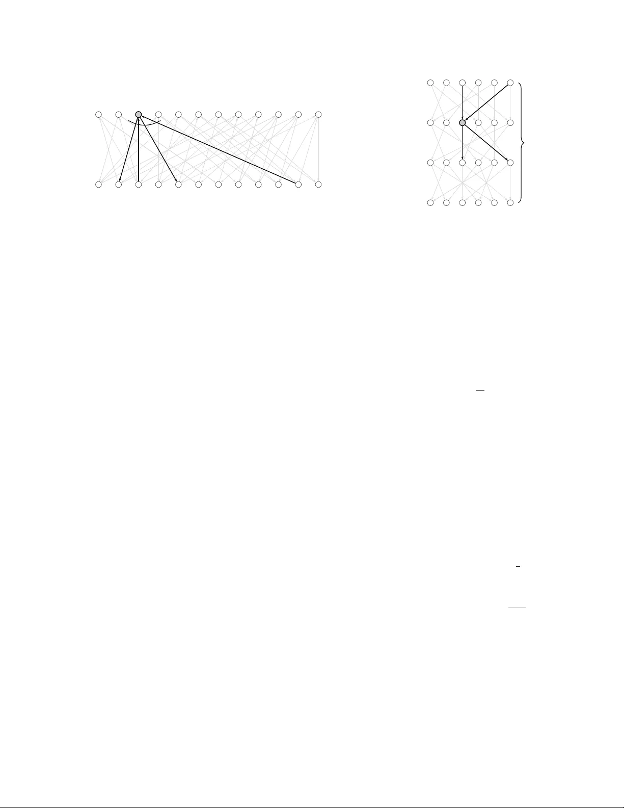
Mark o v Chains with Rewinding Amir Azarmehr ∗ Soheil Behnezhad ∗ Alma Ghafari ∗ Madh u Sudan † Abstract Motiv ated by techniques developed in recen t progress on low er b ounds for sublinear time algorithms (Behnezhad, Roghani and Rubinstein, STOC 2023, F OCS 2023, and STOC 2024) w e in tro duce and study a new class of r andomize d algorithmic pro cesses that we call “Marko v Chains with Rewinding”. In this setting an agen t/ algorithm in teracts with a (partially observ- able) Mark o vian r andom ev olution b y perio dically/strategically rewinding the Mark ov chain to previous states. Dep ending on the application this may lead the evolution to desired states faster, or allo w the agent to eﬃciently learn or test properties of the underlying Marko v chain that may b e infeasible or ineﬃcien t with passive observ ation. W e study the task of identifying the initial state in a giv en partially observ able Marko v c hain. Analysis of this question in sp eciﬁc Marko v chains is the central ingredient in the ab o ve cited works and we aim to systematize the analysis in our work. Our ﬁrst result is that an y pair of states distinguishable with an y rewinding strategy can also be distinguished with a non-adaptive rewinding strategy (i.e., one whose rewinding choices are predetermined b efore observing any outcomes of the chain). Therefore, while rewinding strategies can b e shown to b e strictly more p o werful than passiv e strategies (i.e., those that do not rewind bac k to previous states), adaptivit y does not giv e additional p o w er to a rewinding strategy in the absence of eﬃciency considerations. The diﬀerence b ecomes apparent how ever when w e in tro duce a natural eﬃciency measure, namely the query c omplexity (i.e., the num b er of observ ations they need to identify distinguish- able states). Our second main contribution is to quantify this eﬃciency gap. W e presen t a non-adaptiv e rewinding strategy whose query complexity is within a p olynomial of that of the optimal (adaptive) strategy , and sho w that such a p olynomial loss is necessary in general. ∗ Northeastern Univ ersity . Supp orted in part by NSF CAREER Aw ard CCF-2442812 and a Go ogle Research Aw ard. Emails: { azarmehr.a, s.behnezhad, ghafari.m } @northeastern.edu † Sc ho ol of Engineering and Applied Sciences, Harv ard Universit y , Cam bridge, Massach usetts, USA. Supported in part b y a Simons In vestigator Award, NSF Award CCF 2152413 and AFOSR a ward F A9550-25-1-0112. Email: madhu@cs.harvard.edu Con ten ts 1 In tro duction 1 1.1 Our Contributions . . . . . . . . . . . . . . . . . . . . . . . . . . . . . . . . . . . . . 2 1.2 Related W ork . . . . . . . . . . . . . . . . . . . . . . . . . . . . . . . . . . . . . . . . 3 1.3 Connection to Sublinear-Time Graph Algorithms . . . . . . . . . . . . . . . . . . . . 4 2 Motiv ating Examples & T ec hnical Ov erview 5 2.1 Example 1: The non-trivial p o wer of (non-adaptiv e) rewinding . . . . . . . . . . . . 5 2.2 Example 2: The p o w er of adaptivity . . . . . . . . . . . . . . . . . . . . . . . . . . . 6 2.3 T ec hnical Ov erview . . . . . . . . . . . . . . . . . . . . . . . . . . . . . . . . . . . . . 7 3 The F ormal Mo del 10 3.1 P artitions . . . . . . . . . . . . . . . . . . . . . . . . . . . . . . . . . . . . . . . . . . 11 4 A P olynomially Optimal Non-Adaptive Algorithm 12 4.1 A Non-Adaptive Algorithm with P olynomial Queries . . . . . . . . . . . . . . . . . . 12 4.2 An Informal Ov erview of the Algorithm . . . . . . . . . . . . . . . . . . . . . . . . . 13 4.3 The F ormal Argumen t . . . . . . . . . . . . . . . . . . . . . . . . . . . . . . . . . . . 13 5 The P olynomial Gap of Adaptivit y 18 5.1 The Adaptive Algorithm . . . . . . . . . . . . . . . . . . . . . . . . . . . . . . . . . . 19 5.2 The Non-Adaptive Low er Bound . . . . . . . . . . . . . . . . . . . . . . . . . . . . . 20 6 Generalit y of Canonical Marko v Chains 21 6.1 Adaptiv e Query Complexity . . . . . . . . . . . . . . . . . . . . . . . . . . . . . . . . 22 6.2 Non-Adaptiv e Query Complexity . . . . . . . . . . . . . . . . . . . . . . . . . . . . . 24 A F urther Connections to Sublinear-Time Graph Algorithms 28 1 In tro duction In this work, w e formally deﬁne and study a new class of pro cesses in volving in teraction b et w een randomness and algorithms. In these processes, that w e call Markov chains with r ewinding , a partially observ able Mark ov c hain in teracts with an algorithmic agent that has the abilit y , at an y p oin t in time, to rewind the Mark ov c hain to a previous p oin t of time. W e study the problem of identifying the initial state in this model, where the goal is for the algorithm to use the observ ations and the pow er of rewinding to iden tify a giv en (hidden) initial state. P artially observ able Mark ov chains form a well-established elemen t of the to olkit in computing and arise in b oth the design and analysis of algorithms. Rewinding of Marko v c hains captures a natural abilit y of algorithms that w ork with Marko v c hains, and as a result, they hav e o ccurred implicitly in a v ariet y of settings (an o verview is given in Section 1.2 ). This is highligh ted cen trally in a class of applications of Marko v chains with rewinding to sub- line ar time algorithms . F or the maximum matc hing problem, Behnezhad, Roghani, and Rubinstein [ 7 , 6 , 8 ] pro ve strong lo wer b ounds on the query complexit y , and hence running time, of sublin- ear time algorithms b y using Marko v chains with rewinding to mo del sublinear algorithms, and then analyzing these chains. Recent w orks on non-adaptive sublinear lo w er b ounds follow similar paradigms, while not explicitly deﬁning a Marko v c hain [ 4 , 24 ]. Additionally , low er b ounds for other graph problems in the sublinear-time mo del, such as edge orientation [ 21 ] and acyclicity [ 10 ], can also be view ed as instances of this general model. Despite the prev alence of this phenomenon, rewinding do es not app ear to hav e b een studied formally in the literature and in particular tools to analyze the pow er (and limitations) of Mark ov c hains with rewinding hav e been ad-ho c. Our w ork is motiv ated principally b y these and aims to build a more systematic toolkit for such analysis. Mark o v chains with rewinding: W e start with an example to illustrate the problem. Consider the partially observ able Mark ov chain depicted b elo w, where the only observ able v ariable is the color of the curren t state (i.e., whether it is in { a, a ′ , b, b ′ } or { s } ). The initial state is promised to b e either a or a ′ , and our goal is to iden tify this initial state. a b s b ′ a ′ 1 2 1 2 1 1 1 2 1 2 1 First, note that “passive observ ations” cannot distinguish a from a ′ : Whether we start from a or a ′ , it takes exactly Geometric(1 / 2) + 1 steps until w e reac h s and remain there forever. But supp ose w e are allo wed to r ewind bac k to an y previous state at any time. In this case, we can run the Mark ov c hain for one step to reach state X , and then run D indep enden t steps from X for a suﬃcien tly large D . The idea is that if X = b ′ (whic h implies the initial state is a ′ ), then it will most likely ha v e a mix of s and not s next steps, whereas if X ∈ { a, b } (implying that the initial state is a ) all next steps will b e the same. The following ﬁgure illustrates this. 1 s s s Initial state m ust be a ′ s s s s s s Initial state is a with probability 1 − 2 − D +1 > 0 . 96 . W e no w presen t a more general description of the model, deferring its formalization to Section 3 . The input consists of a partially observ able Mark ov chain M , t wo candidate initial states a and a ′ , and a hidden initial state X 0 ∈ { a, a ′ } . The algorithm in teracts with the Marko v c hain through the hidden initial state X 0 . It can either draw states according to the transition probabilities, or rewind the state to an earlier point in time. The drawn states { X t } t are hidden from the algorithm, but observ ations { Z t } t are av ailable, where Z t = O ( X t ). Ev entually , the algorithm m ust decide whether the initial state X 0 is a or a ′ , based on the observ ations. W e study the runtime and the n umber of queries (i.e. drawn states) required to do so. Other than the motiv ation from sublinear- algorithm low er b ounds, rewinding formalizes a natural approac h to interacting with Mark ov c hains; v ariations and sp ecial cases ha v e been considered rep eatedly in previous work (see Section 1.2 ). 1.1 Our Contributions Our main focus in this w ork is on the follo wing fundamen tal problem: Given a p artial ly observable Markov chain, c an a ne arly-optimal r ewinding str ate gy b e c ompute d eﬃciently? T o b etter understand this question, w e ﬁrst need to formalize the mo del. W e presen t the formal- ization in Section 3 ; W e deﬁne r ewinding str ate gies and state identiﬁc ation algorithms . Rewinding strategy refers to the c hoice of rewinding times throughout the pro cess. A state iden tiﬁcation al- gorithm computes the rewinding strategy through which it interacts with the partially observ able Mark ov chain, and ultimately identiﬁes the initial state based on the observ ations. W e study and compare the p o wer of adaptive and non-adaptive rewinding strategies for this task, where a non- adaptiv e strategy determines how to rewind indep enden tly of the observ ations. These lead us to our k ey complexit y measures QC M ( a, b ) (resp. NA QC M ( a, b )) for the adaptiv e (resp. non-adaptiv e) query c omplexity of distinguishing state a from b in ch ain M , i.e. the minimum num b er of observ a- tions required by a rewinding strategy to distinguish the t wo states. Query complexity provides a b enc hmark for measuring the eﬃciency of an algorithm, and a means of proving low er bounds for its runtime. W e show that there is indeed a p olynomial-time algorithm for the question stated at the b egin- ning of this section. F ormally , we pro ve the follo wing theorem. Theorem 1.1. Given a p artial ly observable Markov chain M = (Ω , P , O ) , ther e exists a non- adaptive algorithm and a c onstant c = c ( | Ω | ) that c an distinguish b etwe en any two states a, b ∈ Ω in time c · QC M ( a, b ) O ( | Ω | ) . In the statement ab o v e, we let M b e a Mark ov c hain on state space Ω with a sp ecial sink state. The only observ able signal a v ailable to the rewinding algorithm is whether the chain is in the sink 2 state or not (similar to the example in Section 1 ). W e call such Marko v chains c anonic al and sho w that iden tifying the initial state in canonical Mark o v chains is essentially as hard as general partially observ able Marko v c hains (see Section 6 ). Observ e that if non-adaptive algorithms cannot distinguish t w o states a and b of a Mark ov c hain M , then Theorem 1.1 implies that no adaptiv e algorithm can do so either. Therefore, non-adaptive algorithms are as p o werful as adaptive ones in terms of whic h pairs of states they can distinguish. F urthermore, formalized as Theorem 1.2 , we show that the (p olynomial) p o wer of QC M ( a, b ) in Theorem 1.1 is tigh t, up to a constan t, for the run time of non-adaptive algorithms. More sp eciﬁcally , w e presen t a partially observ able Mark o v c hain M and states a and b , where a polynomial gap exists b et w een the adaptiv e and non-adaptive query complexity of distinguishing a and b . Theorem 1.2. Ther e is a choic e of M and p air a, b ∈ Ω such that for some c = c ( | Ω | ) , NA QC M ( a, b ) ≥ c · QC M ( a, b ) (1 − o (1)) | Ω | . This holds for inﬁnitely many choic es of | Ω | and query c omplexities. W e remark that the adaptiv e rewinding strategy presented for this gap can be easily turned in to an algorithm with the same run time. Therefore, the p olynomial gap is also presen t b et w een the optimal adaptiv e and non-adaptiv e run times of state identiﬁcation algorithms. W e lea ve op en the question of whether the n umber of states in the Mark ov c hain can b e remov ed from the run-time exp onen t. An y solution w ould require new techniques and necessarily rely on adaptivit y , as remark ed abov e. F ormally , we ask: Op en Problem 1. Given a p artial ly observable Markov chain M = (Ω , P , O ) , c andidate ini- tial states a, b ∈ Ω , and hidden initial state X 0 ∈ { a, b } , is ther e an adaptive state identiﬁc ation algorithm that suc c essful ly identiﬁes the initial state in time QC M ( a, b ) C wher e c onstant C is inde- p endent of the numb er of states? W e b eliev e it is also interesting to compare non-adaptive algorithms against the b est non- adaptiv e benchmark for future w ork. In particular, we ask: Op en Problem 2. Given a p artial ly observable Markov chain M = (Ω , P , O ) , c andidate initial states a, b ∈ Ω , and hidden initial state X 0 ∈ { a, b } , is ther e a non-adaptive state identiﬁc ation algorithm that suc c essful ly identiﬁes the initial state in time NA QC M ( a, b ) C wher e c onstant C is indep endent of the numb er of states? 1.2 Related W ork W e o verview settings where partially observ able Mark o v chains with rewinding hav e o ccurred nat- urally . A highly prev alen t instance is the folklore metho d of conv erting exp ected run times of al- gorithms in to high probabilit y b ounds by restarting the algorithm when it do es not halt promptly . This is a sp ecial case of rewinding where the underlying state of the algorithm is captured by a Mark ov c hain, and the observ ation is limited to kno wing whether the algorithm has halted or not. Restarting/rewinding can also help b oost the success of algorithms as exempliﬁed in the famed randomized algorithm for 3SA T due to Sc h¨ oning [ 23 ]. In the case of random walks on m ulti- dimensional lattices, Janson and Peres [ 20 ] sho w ed that the exp ected hitting time of the origin is 3 ﬁnite when the algorithm is allow ed to restart the walk back from the starting p oin t. More general forms of rewinding lead to elegan t new approaches to optimization and r andom sampling as in the “Go-with-the-winners” algorithm of Aldous and V azirani [ 1 ]. Selecting which state to contin ue the pro cess from is also studied by Dumitriu, T etali, and Winkler [ 17 ], where the algorithm decides whic h Mark ov chain to adv ance, in order to minimize the exp ected time that one of them reac hes the target state. In crypto gr aphy , rewinding arguments play a celebrated role in pro ving the security of proto cols starting with the seminal w ork of Goldw asser, Micali, and Rac koﬀ [ 19 ]. Rewinding is also a central elemen t in deﬁning strong notions of security as in the notion of “resettable zero kno wledge” due to Canetti, Goldreic h, Goldw asser, and Micali [ 12 ]. 1.3 Connection to Sublinear-Time Graph Algorithms T o further motiv ate our model, w e o verview its connection to sublinear time graph algorithms (or more precisely , lo wer b ounds). Here, we provi de a high-lev el description of this connection in general. Later in Section A , we present an explicit connection to the lo wer b ound for testing acyclicit y . That is, we sho w ho w the lo wer b ound is captured b y Mark o v c hains with rewinding. Let us ﬁrst brieﬂy o v erview the mo del of sublinear-time algorithms for graphs. W e are giv en a graph G = ( V , E ) to whic h w e ha v e adjacency list query access. 1 Eac h query can specify a v ertex v and an integer i ≥ 1. The answ er to suc h a query is the i -th neigh b or of v ertex v stored in an arbitrarily ordered list, or ⊥ if deg( v ) < i . Now, the main question of in terest, is the num b er of suc h queries needed to estimate a prop ert y of the graph. F or example, the works of [ 7 , 6 , 8 ] focus on pro ving lo w er b ounds on the query complexit y of estimating the size of maximum matching in the graph (see also [ 5 , 25 , 22 , 11 ] for some algorithms). Man y other problems can, and hav e b een, studied in this setting, including graph coloring [ 3 ], correlation clustering [ 2 ], metric properties suc h as minimum spanning trees [ 16 , 13 ], Steiner trees [ 15 ], TSP [ 14 , 9 ], and man y others. Remark ably , for man y graph prop erties, w e ha v e had unc onditional query lo wer bounds that can b e matc hed algorithmically with sublinear time algorithms. How ev er, these low er bound arguments are often ad ho c, and there is a lac k of systematic to ols to pro ve them. Our hop e is that our mo del and techniques can serve as a ﬁrst step to wards dev eloping such generic low er b ound to ols. Let us expand on this connection a bit further. T ypically , sublinear time low er b ounds are pro v ed b y sp ecifying tw o distributions D Y E S and D N O of graphs, where graphs drawn from D Y E S ha ve the desired prop ert y and those drawn from D N O do not. The lo w er bound then follows b y sho wing that distinguishing these distributions requires man y queries to the graph. In most cases, these distributions are constructed by ha ving a few groups A 1 , A 2 , . . . , A k that eac h v ertex ma y b elong to and is k ept hidden from the algorithm. The distribution of edges betw een these groups diﬀers in D Y E S and D N O , and th us the task of distinguishing these distributions reduces to identifying these groups. The only useful signal that the algorithm receiv es, and helps in iden tifying the groups, is the v ertex degrees. This is precisely ho w the hard instances of [ 7 , 6 , 8 ] for maxim um matc hings are constructed. Lo wer b ounds for other graph problems in the sublinear-time model, such as edge orien tation [ 21 ] and acyclicit y [ 10 ], can also b e viewed as instances of this general framework. No w note that each group A i can b e vie w ed as a diﬀerent state of the Marko v chain. W e let p ij (i.e., the transition probabilit y from A i to A j ) to b e the fraction of edges of group A i that go to A j , represen ting the fact that a random adjacency list neigh b or of an A i no de b elongs to A j with 1 Another common access model is the adjacency matrix mo del. 4 probabilit y p ij . W e construct these states separately for groups in D Y E S and D N O . Then, assuming that the algorithm cannot ﬁnd cycles (whic h holds in many low er b ounds suc h as [ 7 , 6 , 18 , 10 ]) the task of distinguishing the t w o distributions reduces to distinguishing if the initial state is among the YES states or the NO states of the Mark ov chain. Note, in particular, that b ecause the sublinear time algorithm is not constrained to follo w a single path in the graph and can adaptiv ely mak e adjacency list queries to any previously visited v ertex, this corresponds to a rewinding strategy on the Mark ov chain. Therefore, the study of the pow er and limitations of suc h rewinding strategies for general Mark o v chains closely relates to the query complexit y of sublinear-time graph algorithms, and can serv e as a rich to olkit for pro ving low er b ounds against them. P ap er Arrangement More examples of Marko v c hains with rewinding are presen ted in Section 2 . An o verview of our tec hniques app ears in Section 2.3 . The mo del is formally deﬁned in Section 3 . W e examine state partitions, a key to ol for our algorithm, in Section 3.1 . Theorems 1.1 and 1.2 are pro ven in Sections 4 and 5 respectively . Finally , in Section 6 , w e pro v e the generality of canonical Mark o v c hains. 2 Motiv ating Examples & T ec hnical Ov erview W e start this section b y presen ting examples of rewindable Mark ov chains along with optimal strategies to distinguish b et w een tw o candidate initial states. These examples further clarify the mo del and demonstrate how rewinding strategies can be non-trivial ly eﬀectiv e, and th us hard to pro ve lo w er b ounds against. After these examples, we outline the tec hniques used in our algorithms and analyses. 2.1 Example 1: The non-trivial p o w er of (non-adaptiv e) rewinding a b a ′ b ′ s 1 1 − 1 d 1 d 1 d 1 − 1 d 1 − 1 d 1 d 1 Our ﬁrst example in volv es a simple Mark o v chain on 5 states, inspired by the hard distribution of [ 7 ] for graph matchings. The chain is parameterized b y an in teger d , and its transition probabilities are multiples of 1 /d as illustrated by the arro ws in the ﬁgure. There is a sp ecial sink state s , and the algorithm can only observe whether a state is sink or non-sink. The goal is to distinguish whether the initial state is a or a ′ . W e sho w ﬁrst ho w the natural strategy to distinguish tw o candidate initial states a and a ′ leads to query complexit y e O ( d 2 ). A quic k lo ok at the chain and the rewinding strategy seems to suggest that suc h a d 2 complexit y is essen tial; but we show later that a more sophisticated strategy actually distinguishes a from a ′ in O ( d ) queries. A simple algorithm with e O ( d 2 ) query complexity: W e sa y a no de in the tree is an A -no de if its state is a or a ′ and a B -no de if its state is b or b ′ . First, we claim that giv en a no de v in the tree, w e can determine with probability 1 − ε if it is an A or B no de with O ( d log(1 /ε )) queries—we call this an A / B test. T o do this, note that if v is an A -no de, any child of v is non-sink (sp eciﬁcally , it is a B -no de). Moreov er, if v is a B -node, eac h c hild has a probabilit y of 1 /d of b eing a sink no de. Therefore, op ening O ( d log (1 /ε )) c hildren for a node v is suﬃcient for A / B testing v . 5 q 1 q 2 q 3 q 4 · · · q n − 2 s D 1 2 d  1 − 1 d  / 2 1 2 d  1 − 1 d  / 2 1 2 d  1 − 1 d  / 2 1 2 d  1 − 1 d  / 2 1 2 d  1 − 1 d  / 2 1 1 2 d  1 − 1 d  / 2 1 2 1 2 1 2 1 2 1 2 1 2 Figure 2.1: A canonical Marko v chain for which there is a (large) p olynomial gap b et ween adaptiv e and non-adaptive strategies of distinguishing states q 1 and q 2 . ... ... ... Θ( d log d ) Θ( d log d ) Next, having the A / B test a v ailable to us, w e aim to assert whether a giv en A -no de v has state a or a ′ . T o do so, w e ﬁrst op en d log(1 /ε ) children for v . If v has state a , then all of its c hildren m ust be B -nodes. On the other hand, if v has state a ′ , eac h c hild is an A -no de with probability 1 /d , and so at least one m ust be an A -no de with probabilit y 1 − (1 − 1 /d ) d log(1 /ε ) ≥ 1 − ε . It then suﬃces to run the A / B test on these c hildren to chec k if an y of them is an A no de. This takes total time O ( d 2 log 2 (1 /ε )). Cho osing ε = 1 /d 3 so that all A / B tests are correct w.h.p., we get an ov erall query complexity of O ( d 2 log 2 d ). The ﬁnal queried tree is non-adaptive and is illustrated on the right. ... ... Θ( d ) (for A / B testing) 2 d Impro ving query complexit y to O ( d ) : W e now describe ho w we can impro ve o ver the algorithm ab o v e, and distinguish the a and a ′ states with just O ( d ) queries. Here is the k ey insigh t. Suppose that w e op en a path of length 2 d from the ro ot and let us condition on not seeing the s node at all (whic h happ ens with constan t probabilit y). Then, if w e start from the a state, w e must alternativ ely visit a and b , ﬁnally arriving bac k at a since the length of the path is ev en. Ho wev er, if we start from a ′ , there is a constant probability that w e go from a ′ to a ′ exactly once throughout the process since P ( a ′ , a ′ ) = 1 /d and the length of the walk is 2 d . If this even t happens, we end up in state b ′ . Therefore, it suﬃces to run the A / B test on the last v ertex of the path—if it happens to be B , w e will be sure that w e started from a ′ . Note that the success probability is a small constan t, but we can b oost it b y rep eating this pro cess multiple times. The ﬁgure on the righ t sho ws the ﬁnal query tree (for a single repetition of this pro cess), whic h again is non-adaptiv e. 2.2 Example 2: The pow er of adaptivit y Our second example shows the p o wer of adaptive rewinding strategies compared to non-adaptiv e ones. This example, illustrated in Figure 2.1 , is later used to pro v e a p olynomial gap b et ween the non-adaptiv e and adaptive query complexities in the worst case ( Theorem 1.2 ). W e formalize this in Section 5 , but here provide an intuition of ho w adaptivity helps. 6 Giv en a parameter d ≥ 1, the Marko v c hain is formed by com bining a “simple Mark ov chain” and a “dumm y state”. The simple Marko v c hain consists of a path of states, where each state transitions to the next with probability 1 d , and stays in the same state otherwise. States can b e easily distinguished in the simple Marko v chain using O ( n 2 d ) queries, where n = | Ω | is the n umber of states. T o do so, it suﬃces to tak e random walks from the initial state and examine the time it tak es to mov e to the sink (see Section 5 for the proof ). Ho wev er, when com bined with the dumm y state, every state has a 1 2 c hance of jumping to the dumm y state (otherwise, it pro ceeds as b efore). Then, the dumm y state directly mov es to the sink with probabilit y 1. As all the states hav e the same probability of transitioning to the dummy state, mo ving to the sink through the dumm y state rev eals no information about the initial state. Adaptiv e strategies can easily ﬁlter out the dumm y state. That is, they can simulate a random w alk on the simple Mark ov chain b y chec king if the w alk has transitioned to the dumm y state along the w ay , and rewinding back to the previous step if it has. As a result, adaptive strategies retain the O ( n 2 d ) query complexit y ev en with the dummy state added. The non-adaptive strategies cannot do the same, i.e. they cannot c heck whether a random walk has transitioned to the dummy state on the ﬂy (they can only infer it after all the queries are made). In tuitively , to make up for this, they hav e to tak e many more random w alks from the initial state, so as to guarantee that plent y of them reac h the sink without moving through the dummy state. Therefore, the non-adaptive query complexity suﬀers when the dummy state is added and b ecomes (appro ximately) Ω( d n ). See Section 5 for the pro of. 2.3 T ec hnical Ov erview Recall that our main goal is to bring a systematic understanding of distinguishing tw o candidate initial states in a kno wn Marko v chain. In this section, we pro vide a brief o v erview of our meth- o ds. There are tw o main asp ects associated with our task: (1) computing rewinding strategies to distinguish b et w een tw o initial states, and (2) pro ving lo wer bounds for the query complexit y of this task. T ogether the tw o asp ects allow us to establish the eﬃciency of our algorithm, i.e. that its run time is comp etitiv e with the optimal query complexity . Our approac h to b oth asp ects heavily utilizes partitions of the state set Ω. Let P b e a partition of the states, and for a state a ∈ Ω let P ( a ) denote the “class” of a in P , i.e., the set within the partition P that con tains a . As a subroutine, w e study the problem of iden tifying the class of any giv en (hidden) state in P , i.e., the task of computing P ( X 0 ) for a giv en chain M and partition P (note that this is a generalization of the A/B test in Section 2.1 ). By choosing P carefully , this allo ws us to distinguish b et ween t wo states a, b ∈ Ω. Sp eciﬁcally , it suﬃces to identify the class of the initial state for some partition P that separates a and b , i.e., where P ( a )  = P ( b ). In tuitively , iden tifying the class within a given partition b ecomes more diﬃcult as the partition b ecomes more reﬁned. As an extreme case, the test for the trivial partition P 0 = { Ω \ { s } , { s }} can b e performed without an y further queries in a canonical Mark ov c hain since the partial observ ation at any state determines its class in P 0 . Our k ey tool in the design of algorithms is to assume that for some partition P 1 w e kno w ho w to iden tify the states, and then to use this algorithm to build a more reﬁned partition P 2 where we can identify states. Starting this with the trivial partition, w e can use this metho d to w ork our wa y up to more and more reﬁned partitions, till w e reac h a partition that separates a and b at whic h stage our problem w ould be solv ed. The exact details of 7 this reﬁnement step (and ho w w e estimate their query complexit y) are describ ed b elo w. Recall that the goal of Theorem 1.1 is to dev elop a non-adaptive algorithm that distinguishes b et w een t wo states a and b in time O n (1) · QC M ( a, b ) O ( n ) , where n is the num b er of states and O n (1) suppresses terms dep enden t only on n . T o do so, w e deﬁne a w eighted directed graph on the partitions: Namely , ev ery partition P of Ω is a v ertex of this graph and there is a weigh ted edge b et w een every pair of partitions P 1 → P 2 where P 2 reﬁnes P 1 . The w eights w ( P 1 , P 2 ) are formally deﬁned shortly . In tuitiv ely , the main idea is to get a quan tity that roughly allo ws us to determine the class of the initial state in P 2 using appro ximately w ( P 1 , P 2 ) calls to the class-iden tiﬁer for P 1 . Note that if there is a path P 1 → P 2 → P 3 in this graph, then this amounts to sa ying that classes of P 3 can b e identiﬁed using roughly w ( P 1 , P 2 ) · w ( P 2 , P 3 ) calls to the class iden tiﬁer for P 1 . Th us, giv en this graph, w e can easily devise a non-adaptiv e strategy for distinguishing b et w een a and b . F or every partition P w e compute the minim um distance from the trivial partition P 0 (using this m ultiplicative measure of length of a path), and then use the partition P that separates a from b and has the smallest distance among all such P . In particular, if w e let P 0 , P 1 , . . . , P k = P b e the shortest path to P , the test for each P i can b e recursively p erformed b y calling the tests P i − 1 . This results in a test for P k (whic h recall diﬀeren tiates b et w een a and b ) that uses c ( P k ) = Q 1 ≤ i ≤ k w ( P i − 1 , P i ) tests. F or Theorem 1.1 , w e also need to prov e c ( P k ) ≤ QC M ( a, b ) O ( n ) whic h w e discuss shortly , but ﬁrst we describ e how w e compute w ( P 1 , P 2 ). T o understand ho w a test for P 1 can be used to iden tify the class in P 2 of a giv en state, consider, as a warm-up, the original problem of distinguishing b et w een a and b . Equipped with the test for P 1 , one can diﬀeren tiate b et w een a and b as follo ws: Given a state x ∈ { a, b } , w e tak e man y samples from the next state (rewinding bac k to x after each sample) and examine the distribution of their classes in P 1 . If the distribution of these classes for a and b are δ -apart in total v ariation distance, then x can b e identiﬁed successfully with probability 1 − ε using O (log(1 /ε ) /δ 2 ) samples. A similar approac h can b e tak en to distinguish classes of P 2 (instead of tw o states a and b ). This is again captured b y the total v ariation distance of certain distributions whic h giv es us the w eigh t w ( P 1 , P 2 ) in the graph. Sp eciﬁcally , w e can tak e w ( P 1 , P 2 ) = max c,d : P 1 ( c )= P 1 ( d ) P 2 ( c )  = P 2 ( d ) 1 d P TV ( c, d ) 2 , where for x ∈ { c, d } , and d P TV ( c, d ) denotes the total v ariation distance b et w een next states from c and d when pro jected on P . That is, letting X c and X d b e the next state of the Marko v c hain conditioned on the last state b eing c and d resp ectiv ely , d P TV ( c, d ) := d TV ( P ( X c ) , P ( X d )). Th us, this expression captures the hardest to separate pair of states c and d from diﬀerent classes of P 2 (and not already separated in P 1 ) after taking one step on the Mark ov chain starting at these states, using only a class identiﬁer for P 1 . T urning to our low er bound, recall that w e wish to express the shortest path length in terms of the query complexity , i.e. to prov e that Q 1 ≤ i ≤ k w ( P i − 1 , P i ) is at most O n (1) · ( QC M ( a, b )) O ( | Ω | ) , where P 0 → P 1 · · · → P k is the shortest path found b y our algorithm. The argument has tw o main comp onen ts, giv en a partition P : (1) if tw o states c and d with P ( c ) = P ( d ) are far in terms of d P TV , then P has a small outgoing edge separating c and d , and (2) if ev ery tw o states within the same class of P are close in terms of d P TV , then it is diﬃcult to distinguish any t wo states in the same class of P . Note, in particular, that if such a P do es not separate a and b , then it w ould serve as a “certiﬁcate” for the diﬃculty of distinguishing betw een them. W e b egin b y explaining ho w these comp onen ts can b e applied to obtain upp er b ounds on 8 the shortest path (equiv alently , low er b ounds on the query complexity). Consider an y partition P , where a and b are not separated. Giv en that a and b are distinguishable with QC M ( a, b ) queries, we can emplo y (2) to sho w there are t wo states c and d with P ( c ) = P ( d ) suc h that d P TV ( c, d ) = Ω(1 / QC M ( a, b )). Then, using (1), we can infer that P has an outgoing edge of w eigh t at most O n (1) /d P TV ( c, d ) 2 = O n (1) · QC M ( a, b ) 2 . As a result, we can start at P 0 and iteratively tak e the smallest outgoing edge, whic h has w eight at most O n (1) · QC M ( a, b ) 2 , until w e reac h a partition that separates a and b . The path can take a length of at most n − 1 since each partition is reﬁned b y the next. This giv es us a path of length at most O n (1) · QC M ( a, b ) 2 n from P 0 to a partition that separates a and b . No w w e discuss eac h comp onen t separately . First, consider a partition P with that t wo states c and d in the same class of P that hav e d P TV ( c, d ) = D . Let G be an auxiliary graph where the v ertices are the Marko v c hain states, and tw o states are connected if they are closer than D/n in d P TV . W e construct a reﬁnement P ′ of P b y letting tw o states b e in the same class of P ′ if they are in the same class of P and the same connected comp onen t of G . Observe that P ′ separates c and d since d P TV forms a metric, and c and d are more are D apart, whereas any tw o directly connected states are at most D /n apart. F urthermore, the only states that are newly separated b y P are at least D /n apart. Therefore, P has an outgoing edge of w eight at most ( n/D ) 2 to P ′ . F or the second comp onen t, tak e a partition P where any t wo states in the same class of P are at most θ apart in d P TV . W e sho w that for any tw o states a and b with P ( a ) = P ( b ), it holds QC M ( a, b ) = Ω(1 /θ ). Given t wo possible initial states a and b to distinguish, we consider tw o instances of running the rewinding strategy: one with a , and one with b . Let T a and T b b e the query trees that the rewinding strategy creates in each case. W e couple T a and T b suc h that they lo ok the same to the strategy with a large probabilit y . Here, by lo oking the same, we mean that the states generated in T a and T b yield the same observ ations, i.e. they are b oth sink or non-sink. In addition, the coupling is suc h that T a and T b are isomorphic w.r.t. P , meaning the corresponding no des in T a and T b ha ve states that are in the same class of P , with a large probability . W e construct our couplings in an inductiv e manner. In every step, a state u a ∈ T a and the corresp onding state u b ∈ T b are c hosen b y the rewinding strategy to deriv e the next step. At this p oin t, we need a metho d to couple the next step dra wn from u a and u b suc h that they are b oth sink or non-sink with a large probabilit y . Such a coupling is not possible for arbitrary states u a and u b (e.g. P 0 ( u a ) = P 0 ( u b ) do es not imply the same is true for their next step with a large probability). T o do so, w e emplo y the additional prop ert y that P ( a ) = P ( b ), and sho w that the dra wn states can b e coupled suc h that they are in the same class of P with probabilit y 1 − θ . In tuitively , if a rewinding strategy distinguishes b et ween a and b , it should make at least Ω(1 /θ ), so that the ab ov e sc heme “fails” and the dra wn states are in diﬀeren t classes of P . W e remark that something as strong as the shortest path algorithm is not required for Theo- rem 1.1 . While it is in tuitive to use the shortest path as it corresponds to “the cheapest wa y” for testing P in our graph, something as simple as Prim’s algorithm also works. That is, to pro ve The- orem 1.1 , we essen tially show that there exists a partition P separating a and b which is reachable from P 0 through edges of w eight at most O n (1) · QC M ( a, b ) 2 . Therefore, Prim’s algorithm can ﬁnd suc h a P , by starting from P 0 and in each step, adding the minimum outgoing edge to the tree. Also, note that while the shortest path algorithm may use few er queries in many cases, in the worst case, it uses (asymptotically) the same n um b er of queries as Prim’s algorithm ( Theorem 1.2 ). 9 3 The F ormal Mo del W e use Z ≥ 0 to denote the set of non-negativ e in tegers. W e use d TV ( · , · ) to denote the total v ariation distance b et ween t wo distributions. W e start b y reviewing the standard notions of (partially observ able) Marko v c hains. A sequence of random v ariable X 0 , X 1 , X 2 , . . . with X t ∈ Ω for all t is a Markov chain if there exists a conditional probabilit y distribution P X | Y suc h that for every t ∈ Z ≥ 0 w e hav e X t +1 is distributed according to P X | Y = X t . 2 A sequence Z 0 , Z 1 , . . . with Z t ∈ Σ is a p artial ly observable (p.o.) Markov chain if there exists a Marko v c hain X 0 , X 1 , . . . and a function O : Ω → Σ suc h that Z t = O ( X t ) for all t . (While a general theory w ould allo w probabilistic functions O , w e restrict our atten tion to deterministic functions in this work.) W e refer to Ω as the state space and Σ as the observ able space. Note that a partially observ able c hain M is given b y a triple (Ω , P = P X | Y , O ). Next, we turn to the cen tral ob jects of study in this pap er, namely Marko v chains with rewind- ing. Before doing so, we brieﬂy touc h upon t wo views of a rewinding strategy . The formal view is simply as a function that maps a history of observ ations to a non-negative num b er (which we view as the num b er of steps we rewind the curren t time by). An alternate view is that the rewinding strategy builds a tree where, at eac h time step, the algorithm picks a no de of the curren t tree, and the next time step produces a new child for this node whose state is indep enden t of that of all other nodes, conditioned on the paren t’s state. The follo wing deﬁnition uses the formal view, but w e often switch to the tree view in our analyses. Deﬁnition 3.1 ( Mark o v Chains with Rewinding ) . F or a p artial ly observable Markov chain M = (Ω , P , O ) with observable sp ac e Σ , a r ewinding str ate gy is a function A : Σ ∗ → Z ≥ 0 . A Markov chain M = (Ω , P , O ) in initial state X 0 with r ewinding str ate gy A gener ates a se quenc e of r andom variables Z 0 , Z 1 , Z 2 , . . . , with c omp anion variables X 1 , X 2 , . . . as fol lows: F or every t ≥ 0 , we let Z t = O ( X t ) and X t +1 ∼ P X | Y = X t ′ wher e t ′ = max { 0 , t − A ( Z 0 , . . . , Z t ) } . We say that a se quenc e of r andom variables Z 0 , Z 1 , . . . , is a Markov chain with r ewinding if ther e exists a chain M , an initial state X 0 , and a r ewinding str ate gy A that gener ates this se quenc e. Mark ov c hains with rewinding strictly generalize the class of Marko v chains, whic h corresp ond to p assive observation , i.e., the rewinding strategy A ( · ) is the constan t function 0, or equiv alently , the rewinding tree is a path (and hence “chain”). Another class of rewinding strategies, widely used in algorithm design, picks some threshold τ ∈ Z ≥ 0 and sets A ( Z 0 , . . . , Z t ) = t if t = 0 (mo d τ ) and A ( Z 0 , . . . , Z t ) = 0 otherwise. Equiv alen tly , the rewinding tree consists of paths of length τ in tersecting at the root. Such strategies ma y b e termed r esetting str ate gies . An imp ortan t subclass of strategies which we study in this w ork are non-adaptive rew inding strategies, where A ( Z 0 , . . . , Z t ) = A ′ ( t ), i.e., the rewinding strategy is a ﬁxed function of the length and do es not dep end on the actual observ ations. Note that resettable strategies are sp ecial cases of non-adaptive strategies. A simple example of a non-adaptive rewinding strategy inspired by the “go-with-the-winners” algorithm [ 1 ] is the following: A ( Z 0 , . . . , Z t ) = 0 if t  = 0 (mod τ ) and arg max ℓ { Z t − ℓ } otherwise. That is, the c hain-rewinder seeks to maximize the observ ed v ariable, and once in every τ steps, it rewinds to a previous state with the highest observ able. The main prop ert y of Mark ov chains we explore is the identiﬁability of the initial state. Sp ecif- ically , giv en a p.o. Mark o v c hain M and t wo candidate initial states a, b ∈ Ω, w e ask ho w long 2 W e note that such Marko v chains are called time-invariant since transition probabilities, conditioned on the curren t state, are indep enden t of time. 10 a rewinding strategy has to run (or ho w many “queries” it must mak e to M ) to distinguish b e- t ween these t wo starting states. The follo wing deﬁnition formalizes this notion. It only considers iden tiﬁability from an information-theoretical p oin t of view, i.e. the query complexit y: Deﬁnition 3.2 ( Query Complexity ) . Given a p.o. Markov chain M and r ewinding str ate gy A , let Z a 0 , Z a 1 , Z a 2 , . . . denote the Markov chain with r ewinding obtaine d fr om the initial state X 0 = a and let Z b 0 , Z b 1 , Z b 2 , . . . c orr esp ond to the c ase X 0 = b . We say that ( M , A, a, b ) ar e ( ε, T ) -identiﬁable if d TV (( Z a 0 , . . . , Z a T ) , ( Z b 0 , . . . , Z b T )) ≥ ε . The query complexit y of distinguishing a fr om b in chain M with r ewinding str ate gy A , denote d QC A M ( a, b ) , is the minimum T such that ( M , A, a, b ) ar e (1 / 3 , T ) -identiﬁable. Having this, we deﬁne: • the (adaptive) query c omplexity of distinguishing a fr om b to b e: QC M ( a, b ) = min A QC A M ( a, b ) , • and deﬁne the analo gous notion for non-adaptive r ewinding str ate gies. Namely, NA QC M ( a, b ) = min non-adaptive A QC A M ( a, b ) . W e also consider iden tiﬁabilit y from a computational standpoint. That is, we study the time complexit y for algorithms that iden tify the initial state. Such an algorithm pro duces the rewinding strategy and queries the Mark ov chain ac cordingly . Then, it identiﬁes the initial state based on all the observ ations. W e call suc h algorithms state identiﬁc ation algorithms . Deﬁnition 3.3 ( State Iden tiﬁcation Algorithms ) . The input of a state identiﬁc ation algorithm c onsists of a p.o. Markov chain M = (Ω , P , O ) , two c andidate initial states a, b ∈ Ω , and a hidden initial state X 0 ∈ { a, b } . A n (adaptive) state identiﬁc ation algorithm in every step t ≥ 0 , c omputes the r ewinding str ate gy A ( Z 0 , . . . , Z t ) , after which X t +1 is sample d ac c or ding to P X | Y = X t ′ with t ′ = max { 0 , t − A ( Z 0 , . . . , Z t ) } , and the observation Z t +1 = O ( X t +1 ) is r eve ale d to the algorithm. A non-adaptive algorithm c omputes the r ewinding str ate gy b efor e sampling any states. The algorithm de cides the numb er of steps T , and eventual ly outputs the identiﬁe d initial state ( a or b ). We say the algorithm suc c essful ly identiﬁes the initial state if the output is c orr e ct with pr ob ability 2 / 3 . Finally , we deﬁne a sp ecial sub class that w e refer to as c anonic al p.o. Mark ov chains. While general p.o. Marko v chains are of interest, w e state our results in terms of canonical p.o. Mark o v c hains for simplicit y . W e sho w later, in Theorem 6.2 , that canonical c hains capture all chains in our context. Deﬁnition 3.4 ( Canonical p.o. Mark ov Chains ) . We say that p.o. Markov chain M = (Ω , P , O ) is a canonical p.o. Markov chain if ther e exists a state s ∈ Ω that is a sink state (i.e., P X | Y = s = 1 if X = s and zer o otherwise), and O ( a ) = 1 if a = s and 0 otherwise. Th us, in a canonical p.o. Marko v c hain, the only observ able signal is whether the c hain has reac hed the sink or not; and once one reaches the sink, no further observ ations rev eal information. Suc h c hains are the hardest to learn and hence our fo cus. 3.1 P artitions In the rest of this section, we in tro duce the notion of state partitions, i.e. partitions of Ω, a k ey to ol b oth for designing rewinding strategies to distinguish b et w een states, and pro ving lo wer b ounds on the query complexit y of this task. Throughout the section w e use n as a shorthand for | Ω | , p ( a, b ) for P X | Y = b ( a ), and p ( a, C ) for P b ∈ C p ( a, b ). W e use s to denote the sink state. 11 Deﬁnition 3.5 ( P artition ) . Given a set Ω , a p artition P is a c ol le ction of sets such that e ach element a ∈ Ω app e ars in exactly one set of the p artition. We often r efer to these sets as classes, and use P ( a ) to denote the class of a in P . Deﬁnition 3.6 ( T otal V ariation Distance w.r.t. Partitions ) . F or two states a and b , and a p artition P , the total variation distanc e of P X | Y = a and P X | Y = b w.r.t. to P is d P T V ( a, b ) := 1 2 X C ∈P | p ( a, C ) − p ( b, C ) | = max A ⊆P X C ∈ A p ( b, C ) − p ( a, C ) . Her e, A is a c ol le ction of the classes in P . Lemma 3.7. L et P b e a p artition of Ω . Given two states a and b , and or acle ac c ess to P ( x ) for any state x ∈ Ω , ther e exists a non-adaptive r ewinding str ate gy that suc c essful ly distinguishes b etwe en initial states a and b with pr ob ability 1 − ε using O log 1 /ε  d P TV ( a, b )  2 ! queries. Pr o of. Let d = d P TV ( a, b ), and let A ⊆ P b e the collection of classes where the diﬀerence in the distributions is maximized: A := arg max A ⊆P X C ∈ A p ( b, C ) − p ( a, C ) . Note that by deﬁnition p ( b, A ) − p ( a, A ) = d . Giv en a state x ∈ { a, b } , w e dra w 2 log 1 /ε d 2 samples of the next step of x (according to distribution P X | Y = x ), and let X be the fraction of them that land in A . If the state is a , the exp ected v alue of X is p ( a, A ); if the state is b , the expected v alue is p ( b, A ); and the diﬀerence betw een the t wo is equal to d . W e declare that the state is a if X < p ( a, A ) + d 2 and that it is b otherwise. The probabilit y of error when x = a is equal to: Pr  X ≥ p ( a, A ) + d 2  ≤ exp − 2 · 2 log 1 /ε d 2 ·  d 2  2 ! ≤ ε. Similarly , the probabilit y of error when x = b is equal to: Pr  X < p ( a, A ) + d 2  = Pr  X < p ( b, A ) − d 2  ≤ ε. 4 A P olynomially Optimal Non-Adaptive Algorithm 4.1 A Non-Adaptive Algorithm with P olynomial Queries In this section, we present a non-adaptiv e algorithm that distinguishes any t wo (distinguishable) states a and b of an n -state canonical Mark ov chain M = (Ω , P ) (see Deﬁnition 3.4 ) using O n (1) · QC M ( a, b ) O ( n ) queries, where recall QC M ( a, b ) is the optimal query complexit y of distin- guishing a from b with a p ossibly adaptive rewinding strategy , and O n (1) is used to suppress terms 12 dep enden t only on n . In particular, this implies that the gap b et w een adaptiv e and non-adaptive query strategies is only p olynomial so long as the num b er of states of the Marko v chain is constan t. W e later sho w in Section 5 that this is the b est one can hop e for: there are choices of M , a, b where an y non-adaptiv e rewinding strategy requires QC M ( a, b ) Ω( n ) queries. F ormally , w e show: Theorem 4.1. L et M = (Ω , P ) b e a c anonic al p.o. Markov chain with n = | Ω | states. Ther e is a non-adaptive algorithm ( Algorithm 1 ) that distinguishes any distinguishable states a, b ∈ Ω in time O n (1) · ( QC M ( a, b ) log QC M ( a, b )) 2( n − 2) = O n (1) · QC M ( a, b ) O ( n ) . This is equiv alent to Theorem 1.1 . 4.2 An Informal Ov erview of the Algorithm The algorithm deﬁnes a w eighted directed graph G M = ( V , E ) where eac h v ertex of the graph corresp onds to a partitioning of Ω, the state space of the Mark ov c hain. There is an edge from P ∈ V to P ′ ∈ V iﬀ P ′ is a reﬁnemen t of P . Informally sp eaking, it would be helpful to view eac h partitioning P as a test that reveals which class of P a hidden state belongs to. With this view, w e deﬁne the weigh t w ( P , P ′ ) of the directed edge ( P , P ′ ) ∈ E suc h that it upp er b ounds the cost of solving test P ′ ha ving free access to test P . Once w e deﬁne this graph G M , w e compute the shortest path tree on G M (e.g. using Dijkstra’s algorithm) starting from the trivial partitioning P 0 = { Ω \ { s } , { s }} that only separates the sink from the other states. Let P 0 , P 1 , . . . , P k b e the unique path from P 0 to a partitioning P k . W e will deﬁne the cost of P k as c ( P k ) = k − 1 Y i =0 w ( P i , P i +1 ) . W e pro ve that each test P can indeed b e solved with (sligh tly more than) c ( P ) queries. T o distin- guish state a from b , the algorithm tak es the partitioning P that separates a from b and has the minim um cost c ( P ). Our analysis shows that c ( P ) can b e upp er b ounded b y O n (1) · QC M ( a, b ) O ( n ) . 4.3 The F ormal Argumen t Deﬁnition 4.2 (Source Partition) . The sour c e p artition P 0 is the trivial p artition wher e the sink is a singleton class and al l the r emaining states form another class, i.e. P 0 = { Ω \ { s } , { s }} . F or the purposes of this section, w e only consider the partitions that separate s from every other state, i.e. partitions that reﬁne P 0 . Deﬁnition 4.3 (Partition Graph) . Given a c anonic al Markov chain M = (Ω , P ) , let the p artition gr aph G M b e a weighte d dir e cte d gr aph wher e e ach no de is a p artition of the states Ω . F or a p artition P 1 and a r eﬁnement P 2 , ther e is a dir e cte d e dge fr om P 1 to P 2 with weight w ( P 1 , P 2 ) = max a,b : P 1 ( a )= P 1 ( b ) P 2 ( a )  = P 2 ( b ) 1 /  d P 1 TV ( a, b )  2 . 13 The lengths of the p aths ar e deﬁne d multiplic atively. That is, the length of a p ath is the pr o duct of the weights of its e dges. F or a p artition P , its c ost c ( P ) is e qual to the length of the shortest p ath fr om P 0 to P . Belo w is a formal o verview of the algorithm. The details of using the shortest paths to distinguish b et w een states are given in Lemma 4.8 . W e use the notion of trees for rewinding. That is, if X t is sampled b y rewinding to X t ′ (i.e. according to distribution P X | Y = X t ′ ), then X t ′ is the paren t of X t in the tree. Algorithm 1: A non-adaptive algorithm with p olynomial queries. 1 Input: A Mark o v c hain M = (Ω , P ), and t wo states a and b 2 Let G M b e the partition graph of the Marko v chain as in Deﬁnition 4.3 . 3 Compute the (m ultiplicativ e) shortest path tree on G M ro oted at the trivial partition P 0 . 4 Let P b e a partition separating a and b that minimizes c ( P ). 5 Let P 0 , P 1 , . . . , P k = P b e the shortest path to P . 6 Let ε = Θ n  1 c ( P ) log c ( P )  . 7 Query a tree of heigh t k , where the vertices at height i hav e degree Θ n (log(1 /ε ) · w ( P i − 1 , P i )). 8 Use the observ ations in the tree to identify the class of each vertex at heigh t i in P i recursiv ely (see Lemma 4.8 for the details). T o analyze the query complexity of Algorithm 1 , we show there exists a path of length O n (1) · QC ( a, b ) 2( n − 2) to a partition that separates a and b ( Lemma 4.7 ). Then, w e show ho w this path can b e used to distinguish betw een a and b ( Lemma 4.8 ). First, w e pro v e some auxiliary claims. The follo wing lemma essentially upp er-bounds the w eight of the smallest outgoing edge of a partition P , based on t w o states a and b with P ( a ) = P ( b ). Lemma 4.4. T ake a p artition P and any two states a, b ∈ Ω such that P ( a ) = P ( b ) . Then, ther e exists another p artition P ′ that r eﬁnes P and w ( P , P ′ ) ≤  n − 1 d P TV ( a, b )  2 . Pr o of. Let G b e a graph where eac h node corresp onds to a state. There is an edge b et w een tw o states x and y if d P TV ( x, y ) < d P TV ( a, b ) n − 1 . W e let t wo states x and y b e in the same class of P ′ if and only if they are in the same class of P and in the same connected comp onen t of G . First, observe that a and b are separated by P ′ b ecause they are in diﬀeren t connected com- p onen ts of G . Assume for the sake of contradiction that they are connected by a path in G . The length of this path is at most n − 1, and each edge has a w eight strictly smaller than d P TV ( a,b ) n − 1 . This is a contradiction since d P TV is a metric, and the total length of the path cannot b e smaller than the distance of its endpoints (i.e. a and b ). Also, if tw o states are separated in P , then they are separated in P ′ . Therefore P ′ is a reﬁnemen t of P . Second, for an y tw o states x and y such that P ( x ) = P ( y ) and P ′ ( x )  = P ′ ( y ), it holds that d P TV ( x, y ) ≥ d P TV ( a,b ) n − 1 . Otherwise, there w ould ha ve b een a direct edge b et ween them, and they would 14 ha ve been in the same connected comp onen t of G , whic h contradicts P ′ ( x )  = P ′ ( y ). Therefore, by deﬁnition we hav e w ( P , P ′ ) = max x,y : P ( x )= P ( y ) P ′ ( x )  = P ′ ( y ) 1 /  d P TV ( x, y )  2 ≤ 1 /  d P TV ( a, b ) / ( n − 1)  2 . This concludes the pro of. Corollary 4.5. F or a p artition P , if P has no outgoing e dge of weight at most h in the p artition gr aph, then for any two states a and b in the same class of P , it holds that d P TV ( a, b ) < n − 1 √ h . Pr o of. F ollo ws directly from Lemma 4.4 . The following claim states that if there exists a partition P such that ev ery tw o states in the same class are closer than θ w.r.t. d P TV , then distinguishing any t w o states in the same class of P is diﬃcult (roughly sp eaking, requires 1 /θ queries. Claim 4.6. F or a p artition P that do es not sep ar ate a and b , let θ ( P ) : = max x,y : P ( x )= P ( y ) d P TV ( x, y ) . Then, any (p ossibly adaptive) r ewinding str ate gy that uses Q queries, c an suc c essful ly distinguish b etwe en a and b with pr ob ability at most 1 2 + Q · θ ( P ) 2 . Pr o of. Given a rewinding strategy A that mak es at most Q queries, w e consider the query tree of the strategy when the initial state is a and when it is b , and present a coupling such that the coupled trees are isomorphic (w.r.t. P , meaning the corresp onding nodes are in the same class of P ) with probabilit y at least 1 − Q · θ ( P ). Then it can b e inferred that A cannot distinguish b et ween a and b with probabilit y at least 1 2 (1 − Q · θ ( P )), since the strategy makes the same observ ation as long as the trees are isomorphic w.r.t. P 0 . If the strategy is randomized, we ﬁx its random tape and couple the query trees for eac h p ossible random tap e. That is, we assume without loss of generality that the strategy is deterministic. Considering tw o parallel runs of the rewinding strategy where the initial states are a and b resp ectiv ely , we couple the query trees as follows. W e presen t this coupling step by step based on what the strategy does. In certain cases, we say the coupling has faile d and couple the rest of the pro cess on eac h tree indep enden tly . While the coupling has not failed, the tw o trees are the same w.r.t. to P . That is, they are the same top ologically when the states are ignored, and the states of corresp onding no des in the t wo trees are in the same class of P . Let T a and T b b e the trees obtained in eac h run, and assume that the coupling has not failed so far. Initially , each of the tw o trees is a single vertex with state a or b resp ectiv ely . Observ e that P ( a ) = P ( b ), therefore the trees are indeed the same w.r.t. P in the beginning. Let u a b e a no de of the tree from whic h the strategy draws a child in the next step on T a . Then, the corresp onding no de in T b will b e queried by the strategy in the next step, b ecause the trees are the same w.r.t. P , and as a result, the strategy makes the same observ ations, i.e. the sink and none-sink no des are the same. W e also use u a and u b to indicate the state of the Mark o v c hain at these no des. 15 Since the trees are the same w.r.t. P , it holds that P ( u a ) = P ( u b ), therefore, by the deﬁnition of θ ( P ), it holds d P TV ( u a , u b ) ≤ θ ( P ). As a result, b y the deﬁnition of total v ariation distance, the c hildren dra wn from them u a and u b can b e coupled together such that they are in the same class of P with probabilit y at least 1 − d P TV ( a, b ) ≥ 1 − θ ( P ). In case they are in the same class, w e con tinue the coupling as is. Otherwise, we sa y the coupling has failed, and couple the rest of the pro cess independently for the t w o trees. The probabilit y of failure at every step is at most θ ( P ). As a result, since the rewinding strategy uses at most Q queries, the o v erall probabilit y that the coupling fails is at most Q · θ ( P ). When the coupling does not fail, the rewinding strategy has the same output in the t w o runs b ecause the t w o trees are the same w.r.t. P . That is, giv en the tw o initial states a and b , the output is the same with probability at least 1 − Q · θ ( P ). Therefore, for one of a and b the output is incorrect with probability at least 1 2 (1 − Q · θ ( P )). This concludes the proof. Com bining Corollary 4.5 and Claim 4.6 , for a partition P with P ( a ) = P ( b ), w e can upp er- b ound the smallest outgoing edge of P , and pro ve there exists a short path from P 0 to a partition that separates a and b . Lemma 4.7. Ther e exists a p ath of length O n (1) · QC ( a, b ) 2( n − 2) fr om P 0 to a p artition that sep ar ates a and b . Pr o of. T o pro v e a path exists, let S be the set of partitions that are reachable from the source partition P 0 using edges of w eigh t at most h = (3( n − 1) QC ( a, b )) 2 = O n (1) · ( QC ( a, b )) 2 . T ake a partition P ∈ S that has no outgoing edges inside S . Suc h a partition can b e found b ecause an edge P 1 → P 2 can exist only if P 2 reﬁnes P 1 . W e show that a and b are separated in P , and conclude that the shortest path from the source partition to P has length at most h n − 2 . Assume for the sak e of contradiction that a and b are not separated in P . By the c hoice of P , it has no outgoing edges of w eigh t at most h . By Corollary 4.5 , it holds that θ ( P ) < n − 1 √ h ≤ 1 3 QC ( a, b ) . Since P do es not separate a and b , Claim 4.6 implies that any rewinding strategy which uses QC ( a, b ) queries can distinguish b et w een a and b with probability at most 1 2 + QC ( a, b ) · θ ( P ) 2 < 2 3 . This is a contradiction since b y deﬁnition there exists a rewinding strategy distinguishing betw een a and b with QC ( a, b ) queries and success probabilit y 2 3 . Finally , observ e that P is reac hable from the source partition using at most n − 2 edges of w eight at most h . W e ha ve already shown there exists a path consisting of edges of weigh t at most h from the source partition to P . The n um b er of edges in this path is at most n − 2 b ecause eac h partition in the path is a reﬁnemen t of the previous one. Hence the length is at most h n − 2 = (3( n − 1) QC ( a, b )) 2( n − 2) = O n (1) · QC ( a, b ) 2( n − 2) . This concludes the pro of. The follo wing lemma describes how a path of length Q can b e used to distinguish the states with (slightly more than) Q queries. 16 Lemma 4.8. Given a p ath P 0 , P 1 , . . . , P k of length Q , one c an identify the class of the initial state in P k with O n (1) · Q log k Q queries, 3 using a non-adaptive tr e e of height k wher e on the i -th level the de gr e e of every no de is chosen pr op ortional ly to w ( P i − 1 , P i ) and the class of e ach no de on that level is determine d w.r.t. P i . Pr o of. Let P 0 , . . . , P k b e a path of length Q . First, assuming that giv en a state a , we hav e oracle access to P k − 1 ( a ), we recall a subroutine that can identify the class of a state in P k b y drawing c hildren from it and observing their class in P k − 1 . T o do so, w e sho w ho w to distinguish betw een an y t w o states a and b that are in diﬀeren t classes of P k . Let d = d P k − 1 TV ( a, b ) If a and b are also in diﬀerent classes of P k − 1 , then w e can distinguish b et w een them simply b y accessing their class in P k − 1 for free. Otherwise, w e can inv ok e Lemma 3.7 to distinguish betw een a and b b y dra wing 2 log 1 /ε d 2 samples of the next s tep and lo oking at their class in P k − 1 . Giv en any state x , to iden tify its class in P k , we p erform the abov e test for ev ery pair ( a, b ) suc h that P k ( a )  = P k ( b ). A state a is called a “winner” if for ev ery state b with P k ( a )  = P k ( b ) the test ( a, b ) outputs a . W e report that x is in the class C ∈ P k if there exists a winner state in C . Assuming all the tests in volving x were carried out successfully , only P k ( x ) con tains a winner, and P k ( x ) is determined correctly . The total n umber of queries to iden tify the class of a state in P k is the n umber of tests ( n 2 ) times the n umber of queries p er test ( 2 log 1 /ε d 2 ). Also, it holds b y deﬁnition: 1 d 2 ≤ w ( P k − 1 , P k ) . Therefore, the total num b er of queries is at most 2 n 2 · log(1 /ε ) · w ( P k − 1 , P k ) . So far, we ha v e assumed oracle access to the class of a state in P k − 1 . T o lift this assumption, w e simply p erform this pro cedure recursively . That is, to obtain for a state s , its class in P k − 1 , we dra w a n umber of c hildren and lo ok at their classes in P k − 2 , and so on. As a result, we get a tree, where the total num b er of queries is: k Y i =1 2 n 2 · log(1 /ε ) · w ( P i − 1 , P i ) ≤  2 n 2 log(1 /ε )  k k Y i =1 w ( P i − 1 , P i ) ≤  2 n 2 log(1 /ε )  k · Q. Here, the ﬁrst inequality follows from rearranging the terms, and the second inequalit y holds by the deﬁnition of Q (the length of the path). It remains to set the v alue of ε suc h that all tests are carried out successfully with the desired probabilit y of 2 3 . Applying the union b ound, the probability that at least one of the tests is unsuccessful is at most ε ·  n 2 log(1 /ε )  k · Q. 3 recall k ≤ n − 2 17 By letting ε = Θ  1 n 2 k Q log( n 2 k Q )  , this probability b ecomes smaller than 1 / 3. Plugging ε bac k in, the total num ber of queries this metho d uses to iden tify the class of an y state in P k with success probabilit y 2 / 3 is: O   2 n 2 log(1 /ε )  k · Q  = O n (1) · Q log k Q. Finally , we put Lemmas 4.7 and 4.8 together to deriv e Theorem 4.1 . Pr o of of The or em 4.1 . By Lemma 4.7 , for an y t wo states a and b , there exists a path of length at most QC ( a, b ) 2( n − 2) ending at a partition that separates a and b . Therefore, the partition P obtained by computing shortest paths in step 4 of the algorithm has cost at most QC ( a, b ) 2( n − 2) . Lemma 4.8 sho ws ho w the shortest path to P can b e used in steps 7 - 8 , to iden tify the class of the initial state in P using O n (1) · ( QC ( a, b ) log QC ( a, b )) 2( n − 2) queries, hence distinguishing b et ween a and b . Regarding the runtime, observ e that the strategy is implicitly (non-adaptively) computed in O n (1). The num b er of state partitions (n umber of v ertices in G M ) is at most n n = O n (1). F or an edge P → P ′ , the w eight can b e computed in time O ( n 3 ) by iterating ov er ev ery relev ant pair of states and computing the distance d P TV in O ( n ). Then the shortest path tree can be computed using a polynomial-time algorithm (e.g. Dijkstra’s). After the shortest path is computed, the degree on eac h lev el of the query tree is determined. F or eac h no de of height i , its calls in P i can b e determined in time O (2 n 2 · log (1 /ε ) · w ( P k − 1 , P k )), i.e. prop ortional to the degree. Therefore, the run time of the algorithm is O n (1) · ( QC ( a, b ) log QC ( a, b )) 2( n − 2) = O n (1) · ( QC ( a, b )) O ( n ) . 5 The P olynomial Gap of Adaptivit y In this section, we pro ve the follo wing theorem whic h directly implies Theorem 1.2 . Theorem 5.1. F or any p ar ameters n, d ≥ 1 , ther e exists a c anonic al Markov chain M = (Ω , P ) with n = | Ω | states and two states a, b ∈ Ω such that QC M ( a, b ) = O ( n 2 d ) , NA QC M ( a, b ) = Ω( d (1 − o (1)) n ) . W e remark that the optimal rewinding strategy , whic h distinguishes b et w een a and b using O ( n 2 d ) queries, can b e trivially turned in to an algorithm with the same run time. Therefore, Theorem 5.1 implies the same gap betw een the optimal adaptiv e and non-adaptiv e run times of state identiﬁcation algorithms. As such, in this section, w e abuse the notation and use the terms rewinding strategy and algorithm in terc hangeably . W e prov e the claim giv en d > 0 and, the Marko v chain M appeared in Figure 2.1 . In this Mark o v c hain, the states form a directed path tow ard the sink state, with states lab eled as q 1 , ..., q n − 2 from left to right. W e label the last state as D . F or all i ∈ [ n − 3], state q i go es to q i +1 with probability 1 2 d . The state q n − 2 go es to the sink state s with the same probabilit y . Eac h state in q 1 , ..., q n − 2 go es to itself with probabilit y  1 − 1 d  / 2. All q 1 , ..., q n − 2 go to the state D with probabilit y 1 2 , while state D go es to the sink with probability 1. W e prov e that there exists an adaptiv e algorithm distinguishing q 1 and q 2 with O ( n 2 d ) queries, while an y non-adaptive algorithm needs at least Ω( d (1 − o (1)) n ) queries. The intuition is as follo ws. An adaptiv e algorithm can easily test whether each new state op ened is the D state or not by 18 simply doing a test with constan t queries, and op ening another c hild instead to con tinue its path. This is not possible for non-adaptiv e algorithms that come across the D state with probabilit y 1 2 , and when this happ ens the algorithm intuitiv ely loses any information on the state it started from. So it needs a lot of paths to account for this loss of information. 5.1 The Adaptive Algorithm Lemma 5.2. Ther e exists an adaptive algorithm that distinguishes q 1 and q 2 in Markov chain M of Figur e 2.1 with O ( n 2 d ) queries. Pr o of. T o describ e the algorithm, we ﬁrst in tro duce a bo olean D -test that can distinguish the state D from any other state. Giv en an unknown state a , w e tak e a constant num b er of children of a . If all of these c hildren are the sink, then a is the D state; otherwise, a is not the D state. Note that the algorithm encoun ters state D in only an ε fraction of its queries. No w w e describ e the adaptiv e algorithm A as follo ws: • Giv en an initial state a ∈ { q 1 , q 2 } , op en a c hild c of a . • If c is not a sink, run the D -test on c . – If the D -test is p ositiv e (indicating c is D ), then op en another child from the parent of c . – If the D -test is negative, con tinue to open a c hild from c . This algorithm will pro duce a path from a to the sink that a voids state D . The length of this path helps determine whether the algorithm started at q 1 or q 2 . Let E 1 and E 2 represen t the exp ected lengths of suc h paths when starting from q 1 and q 2 , resp ectiv ely , and let V ar 1 and V ar 2 denote the v ariances of these path lengths. Note that the paths do not include encoun ters with state D or additional queries from the D -tests. Since each transition has a probability of 1 2 d of moving to the next state in the sequence, E 1 = ( n − 2) · d 2 and E 2 = ( n − 3) · d 2 . The v ariance of a path length in b oth cases, V ar 1 and V ar 2 , is b ounded b y the v ariance of the sum of ( n − 2) or ( n − 3) indep enden t geometric random v ariables with success probability 1 2 d . W e ha ve V ar 1 = 2( n − 2)(1 − 1 /d ) (1 /d 2 ) ≤ 2 nd 2 and V ar 2 = 2 ( n − 3)(1 − 1 /d ) (1 /d 2 ) ≤ 2 nd 2 . Let X 1 , . . . , X k denote the lengths of the n paths generated b y A . T o distinguish b et ween q 1 and q 2 , we compare the sample mean of path lengths, X = 1 k P k i =1 X i , to E 1 and E 2 . Let σ b e the standard deviation of random v ariable X . W e ha ve σ 2 ≤ nd 2 /k . By applying Cheb yshev’s Inequalit y to the sample mean X , when the starting state is q 1 , we hav e Pr  | X − E 1 | ≥ d/ 2  ≤ 4 σ 2 d 2 ≤ 8 n k . 19 Similarly for the case that the starting state is q 2 w e ha v e Pr  | X − E 2 | ≥ d/ 2  ≤ 4 σ 2 d 2 ≤ 8 n k . T o distinguish b et w een the tw o exp ected path lengths E 1 and E 2 with high probability , w e w ant the sample mean X to be close to E 1 or E 2 dep ending on the starting state. Thus, w e set k = 100 n . In the case that the starting state is q 1 with probabilit y 2 / 3 w e hav e | X − E 1 | ≤ d/ 2, and if the starting state is q 2 with high probability w e ha v e | X − E 1 | ≤ d/ 2. Therefore, the algorithm succeeds with probabilit y 2 / 3. The total size of the tree that this algorithm op ens is O ( nd · n ) = O ( n 2 d ), and with probability at least 2 3 , this algorithm will distinguish b et w een q 1 and q 2 . 5.2 The Non-Adaptive Lo w er Bound Lemma 5.3. Any non-adaptive algorithm distinguishing q 1 and q 2 in Markov chain M of Figur e 2.1 ne e ds Ω( d (1 − o (1)) n ) queries. Pr o of. Assume there exists a non-adaptiv e algorithm A designed to distinguish the states q 1 and q 2 in the Marko v chain M . Giv en either q 1 or q 2 as the initial state, A generates a tree T that corresp ond to states of the Marko v chain. F or b oth starting states q 1 and q 2 , the tree T has the same structure due to the non-adaptive nature of A . W e will construct a coupling of the execution of A when starting from q 1 v ersus starting from q 2 , to sho w that the algorithm needs a large num b er of queries to successfully distinguish b et ween the tw o initial states. Let T denote the tree generated by A , with eac h no de in T represen ting a queried state in the Mark ov c hain. W e deﬁne the t wo coupled v ersions of the tree as T q 1 starting at q 1 , and T q 2 , starting at q 2 . W e deﬁne the coupling as follows. If T q 1 remains in its curren t state, then T q 2 also self-lo ops in its curren t state. If T q 1 transitions to the next state to the righ t (from q i to q i +1 ), then T q 2 mak es the same transition to the right. If T q 1 transitions to the dummy state D , then T q 2 also transitions to D . If the sink s is reached in either tree, but not the other, w e sa y the trees ha ve decoupled, as this rev eals information about the starting state. Since w e coupled reac hing to the state D , the decoupling happ ens when in T q 2 there is a transition from q n − 2 to the s and T q 1 transitions from q t − 3 to q n − 2 . Let p decouple denote the probability that the trees T q 1 and T q 2 decouple within a path of length k . Sp eciﬁcally , p decouple is the probabilit y that one of the trees reac hes s while the other do es not: p decouple = Pr(reac h s in T q 2 but not in T q 1 ) . By the structure of M the probability that using a path of length k starting from q 2 , we reach sink is p decouple ≤  1 2  k min  k n − 2   1 d  n − 2 , 1 ! . 20 W e prov e that p decouple ≤ 1 d (1 − o (1)) n , in the case that k > 2 n log( d ), since min(  k n − 2   1 d  n − 2 , 1) ≤ 1, w e ha v e p decouple ≤ ( 1 2 ) k ≤ e − n log( d ) ≤  1 d  n . In the case that k ≤ 2 n log ( d ), p decouple ≤  k n − 2   1 d  n − 2 ≤  ek n  n  1 d  n − 2 ≤ (2 e log( d )) n  1 d  n − 2 ≤  1 d  (1 − o (1)) n . No w since, p decouple ≤ 1 d (1 − o (1)) n , using union bound on all the paths in tree T ,the total prob- abilit y that decoupling happ ens is at most | T | d (1 − o (1)) n , if | T | < d (1 − o (1)) n / 3, then the coupling fails with probabilit y at most 1 / 3 and the algorithm A distinguishes q 1 and q 2 with probabilit y at most 1 / 3. Therefore, an y non-adaptive algorithm that distinguishes q 1 and q 2 should use a tree of size Ω( d (1 − o (1)) n ). Pr o of of The or em 5.1 . F ollows from combining Lemmas 5.2 and 5.3 . 6 Generalit y of Canonical Marko v Chains In this section, w e sho w that iden tifying the initial state of a canonical Mark ov chain ( Deﬁnition 3.4 ) is (essentially) as hard as the same task in an y partially observ able Mark o v c hain via a reduction. That takes in to accoun t both the query complexit y of the rewinding strategy and the runtime of the algorithm. F or a state iden tiﬁcation algorithm A w e write T( A ) for the time it spends outside the oracle that samples the next state. In the generalized version, a Marko v c hain M = (Ω , P ) is complemen ted b y an observ ation function O : Ω → Σ, i.e. ev ery state x ∈ Ω in the Marko v c hain outputs an observ ation O ( x ) ∈ Σ. The states remain hidden, but in every step, the algorithm can see the observ ation and use it to iden tify the initial states. A canonical Mark o v c hain can b e expressed in this generalized v ersion b y letting the set of p ossible observ ations b e Σ = { 0 , 1 } , and letting O ( x ) = 1 ( x = s ) where s is the sink state. That is, the observ ation made at an y state is whether it is the sink state. First, W e sho w that any adaptiv e strategy taking Q queries in the generalized model can b e emulated in the canonical Mark ov chain using O ( | Σ | Q ) queries. Secondly , w e sho w that for non-adaptiv e algorithms, the gap b et ween the query complexity of canonical and generalized Mark o v c hains is at most near-quadratic. F ormally , w e deﬁne a reduction from a generalized Marko v c hain M to a canonical Marko v c hain ˆ M b elo w. See Figures 6.1 and 6.2 for an example of this reduction. Deﬁnition 6.1 ( Reduction to Canonical Mark o v c hains ) . L et M = (Ω , P ) b e a Markov chain with state sp ac e Ω , tr ansition matrix P , and an observation function O : Ω → Σ that maps e ach state to an observable output. L et the emulate d Markov chain of M b e a c anonic al Markov chain ˆ M = ( ˆ Ω , ˆ P ) with state sp ac e ˆ Ω and tr ansition matrix ˆ P as fol lows: F or e ach state x ∈ Ω , ther e exists a unique c orr esp onding state ˆ x = ϕ ( x ) in ˆ Ω , wher e ϕ : Ω → ˆ Ω is an inje ctive mapping. L et k = | Σ | and and Σ = { σ 1 , . . . , σ k } . Given a p ar ameter 0 < q < 1 we have 21 1. F or every p air of states x, x ′ ∈ Ω with tr ansition pr ob ability p x,x ′ in P , we intr o duc e an extende d p ath in ˆ M c onsisting of a series of interme diate states d x,x ′ 1 , d x,x ′ 2 , . . . , d x,x ′ k − 1 with tr ansition pr ob ability 1 b etwe en c onse cutive states, such that ˆ x tr ansitions to ˆ x ′ via these interme diate states. ˆ x tr ansitions to d x,x ′ 1 with pr ob ability q p x,x ′ and d x,x ′ k − 1 tr ansitions to ˆ x ′ with pr ob ability 1 . 2. T o emulate the observation function O , we intr o duc e a set of sp e cial states σ 1 , σ 2 , . . . , σ k = s in ˆ M , e ach r epr esenting a unique observation in Σ . s is the sink state of the c anonic al Markov chain ˆ M . Each state ˆ x ∈ ˆ Ω in ˆ M tr ansitions to a sp e cial state c orr esp onding to its observation in M with pr ob ability 1 − q . Sp e cial state σ i tr ansitions to σ i +1 with pr ob ability 1 for i ∈ [ k − 1] . s 1 s 2 s 3 p 12 p 21 p 23 p 31 Figure 6.1: Represen ts a general Marko v chain M with observ ations Σ = { σ 1 , σ 2 , σ 3 } , where O s 1 = σ 1 , O s 2 = σ 2 , and O s 3 = σ 2 . ˆ s 1 d s 1 ,s 2 1 d s 1 ,s 2 2 ˆ s 2 d s 1 ,s 3 1 d s 1 ,s 3 2 ˆ s 3 d s 2 ,s 1 1 d s 2 ,s 1 2 d s 2 ,s 3 1 d s 2 ,s 3 2 σ 1 σ 2 s q p 12 1 1 q p 31 1 1 q p 23 1 1 q p 13 1 1 1 1 1 − q 1 − q 1 − q Figure 6.2: Represents a canonical Marko v c hain ˆ M , with parameter 0 < q < 1, where there is an injection ϕ that reduces distinguishing states a and a ′ in M to distinguishing ϕ ( a ) and ϕ ( a ′ ) in ˆ M . 6.1 Adaptiv e Query Complexit y Theorem 6.2. L et M = (Ω , P ) b e a Markov chain in the gener alize d mo del with an observation function O : Ω → Σ , Then, ther e exists a c anonic al Markov chain ˆ M = ( ˆ Ω , ˆ P ) states and an inje ctive mapping of the states ϕ : Ω → ˆ Ω , such that for any two states a, a ′ ∈ Ω , QC ˆ M ( ϕ ( a ) , ϕ ( a ′ )) = Θ  | Σ | QC M ( a, a ′ )  . Pr o of. Let Mark o v c hain ˆ M = ( ˆ Ω , ˆ P ), be the emulation of M with parameter q = 1 / 2. No w w e show QC ˆ M (ˆ a, ˆ a ′ ) ≤ O  | Σ | QC M ( a, a ′ )  , 22 where a, a ′ ∈ S , ˆ a = ϕ ( a ), and ˆ a ′ = ϕ ( a ′ ). Given an algorithm A that distinguishes b et w een a and a ′ b et w een Q = QC M ( a, a ′ ) queries, w e presen t an adaptiv e algorithm ˆ A in ˆ M using O  | Σ | Q  queries as follo ws. Eac h no de in the query tree of A has a corresp onding no de in the query tree of ˆ A . Initially , the ro ots correspond to each other, and if the root of A is in state x ∈ Ω, then we let the root of ˆ A be in state ˆ x = ϕ ( x ). Whenever a new state is dra wn b y A , we need to em ulate the observ ation. T o do so, ˆ A repeatedly dra ws paths of length at most | Σ | until one of them reac hes the sink. The n umber of paths is constant in exp ectation since we rewind a special state on the ﬁrst step of the path with probabilit y 1 2 . The observ ation can be inferred afterw ard since it is equal to the length of the path that reaches the sink. With the observ ation in hand, A would choose another no de to dra w a child from. T o em ulate this, ˆ A rep eatedly draws paths of length at most | Σ | until one of them do es not reac h the sink. The end of the path corresponds to the c hild no de. Observ e that starting at a no de with state ˆ x (corresp onding to x ), the probabilit y that the no de at the end of the path is in ˆ x ′ (corresp onding to x ′ ) is p xx ′ b ecause we are conditioning on the fact that the path did not mov e to a special state on the ﬁrst step. The exp ected num ber of these paths is also constan t. Therefore, eac h query of A can b e emulated by O ( | Σ | ) queries of ˆ A . T o complete the pro of, we aim to sho w that Ω  | Σ | · QC M ( a, a ′ )  ≤ QC ˆ M ( ϕ ( a ) , ϕ ( a ′ )) . Let ˆ A be a rewinding algorithm on ˆ M that starts at ϕ ( a ) or ϕ ( a ′ ) and distinguishes these t w o states. Let t ′ b e the num ber of queries made b y ˆ A , and let X ′ 0 , . . . , X ′ t ′ b e the observed states in ˆ M with corresp onding observ ations Z ′ 0 , . . . , Z ′ t ′ , where for an y i ∈ [ t ′ ], Z ′ i ∈ { 0 , 1 } . If Z ′ i = 1, then X ′ i is a sink state. Let us deﬁne L ′ i as a set of observ ed states that are in distance i from the ro ot of the query tree of rewinding algorithm A . More formally w e ha v e L ′ 0 = { X ′ 0 } , and for an y i > 0, let L ′ i b e the set of observed states that are a c hild of an y states in L ′ i − 1 . No w w e aim to build a rewinding algorithm A using ˆ A . Let X 0 = X ′ 0 b e the starting state of the algorithm F or any maximal disjoint subtree T ′ that is ro oted at L ′ 1 and T ′ ⊂ L ′ 1 ∪ · · · ∪ L ′ | Σ | , if there exists a state in T ′ with observ ation 1, or the depth of T is less than | Σ | w e do nothing, otherwise w e rewind a child of X 0 . Similarly , let L i denote the states rewinded in A , w e set L 0 = { X 0 } and L 1 as the set of rewinded children of X 0 . No w we build L i inductiv ely such that there is a function S that for any state X ∈ L i , w e hav e S ( X ) as a set of non-sink states in L ′ i ·| Σ | , and each non-sink states in L ′ i ·| Σ | is co vered b y a state in L i . The base Case is i = 0. F or any i > 0, given an y state X ∈ L i and S ( X ) we deﬁne L i +1 as follo ws. Consider the m ax imal disjoin t subtrees T that is ro oted in a state r in L ′ i ·| Σ | +1 and r is a c hild of a state in S ( X ). Also let T b e a sub set of L ′ i ·| Σ | +1 ∪ · · · ∪ L ′ ( i +1) ·| Σ | . Let the set of all suc h subtrees T i . F or each subtree T ∈ T i , if any state in the subtree has an observ ation 1 (i.e., it is a sink state), or if the subtree has depth less than | Σ | , do nothing. Otherwise, rewind a c hild of X in A corresponding to the subtree, and include this child in L i +1 . No w w e prov e A can distinguish betw een a and a ′ . First, note that any state y ∈ L ′ ik , is either the sink or there exists a state x ∈ Ω where ϕ ( x ) = y . Since the length of transition paths for any t wo states ϕ ( x ) and ϕ ( x ′ ) is k for any x, x ′ ∈ Ω. Also, since the transition paths are unique, any 23 subtree T ∈ T i has the same states in one level of tree. Therefore, any suc h tree reveals a transition from x to x ′ if it starts at a child of ϕ ( x ) and at least one path in T ends at ϕ ( x ′ ). In the case that T reaches to the sink, A simply uses the observ ation of the last state. Therefore, if ˆ A can distinguish ϕ ( a ) and ϕ ( a ′ ), A can distinguish b et ween a and a ′ . Note that the size of an y subtree of depth | Σ | is at least | Σ | . Since for any rewinded state in A there exists subtree of depth | Σ | in ˆ A , A can distinguish a and a ′ in QC ˆ M ( ϕ ( a ) ,ϕ ( a ′ )) | Σ | . Remark 6.3. This r e duction pr eserves running time up to the same multiplic ative overhe ad: for any adaptive state identiﬁc ation algorithm A for M that makes Q queries and runs in time T ime ( A ) , ther e is an algorithm ˆ A for ˆ M that runs in time T ime ( A ) + O ( k Q ) , wher e k = | Σ | . A lso, any adaptive algorithm ˆ A for ˆ M with Q ′ queries and time T ime ( ˆ A ) yields an algorithm for M with Ω( Q ′ /k ) queries and time T ime ( ˆ A ) + O ( Q ′ ) . 6.2 Non-Adaptiv e Query Complexit y Theorem 6.4. L et M = (Ω , P ) b e a Markov chain in the gener alize d mo del with an observation function O : Ω → Σ , Then, ther e exists a c anonic al Markov chain ˆ M = ( ˆ Ω , ˆ P ) states and an inje ctive mapping of the states ϕ : Ω → ˆ Ω , such that for any two states a, a ′ ∈ Ω , Ω  | Σ | NA QC M ( a, a ′ )  ≤ NA QC ˆ M ( ϕ ( a ) , ϕ ( a ′ )) ≤ ˜ O  | Σ | NA QC M ( a, a ′ ) 2  . Pr o of. Consider a non-adaptive algorithm A op erating on a Mark ov chain M to distinguish b et w een the states a and a ′ . Given a ﬁxed constant c 1 > 0 and Q as the query complexity of A , let Marko v c hain ˆ M = ( ˆ Ω , ˆ P ), be the emulation of M with parameter q = 1 − c 1 Q . First, we prov e NA QC ˆ M ( ϕ ( a ) , ϕ ( a ′ )) ≤ ˜ O  | Σ | Q 2  . W e build a non-adaptiv e algorithm ˆ A on ˆ M that distinguishes ϕ ( a ) and ϕ ( a ′ ) with ˜ O ( | Σ | Q 2 ) queries. F or an y rewinded state X to Y in A and a ﬁxed constant c 2 > c 1 , w e rewind c 2 Q log ( Q ) paths of size | Σ | . W e pick one of such paths at random to rewind from next, where the last state of the pick ed random path represen ts ˆ Y . Now, at any p oin t that A rewinds Y , ˆ A will rewind ˆ Y . Therefore for an y query in A , ˆ A pro duces c 2 | Σ | Q log ( Q ) queries. T o get to the observ ation of eac h state in ˆ Ω, ˆ A needs to query suc h paths such that at least one of the paths gets to the sp ecial states. The probability that there exists a state queried in A whose random paths in ˆ A do not include a special state is Q (1 − 1 c 1 Q ) c 2 Q log( Q ) ≤ Q exp ( − c 2 Q log ( Q ) c 1 Q ) = Q 1 − c 2 /c 1 . The probability that among the Q pick ed random paths at least one of the random paths is the sp ecial path is ( 1 c 1 Q ) Q = 1 c 1 . By setting c 2 > c 1 > 0 suc h that 1 c 1 , Q 1 − c 2 /c 1 < 1 / 10, the algorithm distinguishes ϕ ( a ) and ϕ ( a ′ ) with high probability . T o complete the pro of, we sho w that Ω  | Σ | · NAQC M ( a, a ′ )  ≤ NA QC ˆ M ( ϕ ( a ) , ϕ ( a ′ )) . The pro of is similar to the lo wer bound of reduction for the adaptiv e algorithm. Ho wev er, we state the proof for the sak e of completeness. 24 Let ˆ A be a rewinding algorithm on ˆ M that starts at ϕ ( a ) or ϕ ( a ′ ) and distinguishes these t w o states. Let t ′ b e the num ber of queries made b y ˆ A , and let X ′ 0 , . . . , X ′ t ′ b e the observed states in ˆ M . Let us deﬁne L ′ i as a set of observ ed states that are in distance i from the ro ot of the query tree of rewinding algorithm A . More formally w e ha v e L ′ 0 = { X ′ 0 } , and for an y i > 0, let L ′ i b e the set of observed states that are a c hild of an y states in L ′ i − 1 . No w we aim to build a rewinding algorithm A using ˆ A . Let X 0 = X ′ 0 b e the starting state of the algorithm F or any maximal disjoint subtree T ′ that is ro oted at L ′ 1 and T ′ ⊂ L ′ 1 ∪ · · · ∪ L ′ | Σ | , if the depth of T is less than | Σ | w e do nothing, otherwise w e rewind a c hild of X 0 . Similarly , let L i denote the states rewinded in A , w e set L 0 = { X 0 } and L 1 as the set of rewinded children of X 0 . No w we build L i inductiv ely such that there is a function S that for any state X ∈ L i , w e hav e S ( X ) as a set of non-sink states in L ′ i ·| Σ | , and each non-sink states in L ′ i ·| Σ | is co vered b y a state in L i . The base Case is i = 0. F or any i > 0, given an y state X ∈ L i and S ( X ) we deﬁne L i +1 as follo ws. Consider the m ax imal disjoin t subtrees T that is ro oted in a state r in L ′ i ·| Σ | +1 and r is a c hild of a state in S ( X ). Also let T b e a sub set of L ′ i ·| Σ | +1 ∪ · · · ∪ L ′ ( i +1) ·| Σ | . Let the set of all suc h subtrees T i . F or eac h subtree T ∈ T i , if the subtree has depth less than | Σ | , do nothing. Otherwise, rewind a c hild of X in A corresp onding to the subtree, and include this c hild in L i +1 . No w w e prov e A can distinguish betw een a and a ′ . First, note that any state y ∈ L ′ ik , is either the sink or there exists a state x ∈ Ω where ϕ ( x ) = y . Since the length of transition paths for an y t w o states ϕ ( x ) and ϕ ( x ′ ) is k for any x, x ′ ∈ Ω. Also, since the transition paths are unique, an y subtree T ∈ T i has the same states in one lev el of the tree. Therefore, any such tree rev eals a transition from x to x ′ if it starts at a child of ϕ ( x ) and at least one path in T ends at ϕ ( x ′ ). In the case that T reac hes the sink, A simply uses the observ ation of the last state. Therefore, if ˆ A can distinguish ϕ ( a ) and ϕ ( a ′ ), A can distinguish b et ween a and a ′ . Note that the size of an y subtree of depth | Σ | is at least | Σ | . Since for any rewinded state in A there exists subtree of depth | Σ | in ˆ A , A can distinguish a and a ′ in NAQC ˆ M ( ϕ ( a ) ,ϕ ( a ′ )) | Σ | . Remark 6.5. If a non-adaptive algorithm A for Markov chain M uses Q queries and runs in time T ime , then the induc e d non-adaptive algorithm b A for ˆ M c an b e implemente d with ˜ O ( kQ 2 ) queries and total running time T ime ( A ) + ˜ O ( kQ 2 ) , wher e k = | Σ | . Also, any non-adaptive ˆ A for ˆ M with Q ′ queries and time T ime ( ˆ A ) yields a non-adaptive algorithm for M with Ω( Q ′ /k ) queries and running time T ime ( ˆ A ) + O ( Q ′ ) . 25 References [1] Da vid J. Aldous and Umesh V. V azirani. ”go with the winners” algorithms. In 35th A nnual Symp osium on F oundations of Computer Scienc e, Santa F e, New Mexic o, USA, 20-22 Novem- b er 1994 , pages 492–501. IEEE Computer So ciet y , 1994. doi: 10.1109/SFCS.1994.365742. URL https://doi.org/10.1109/SFCS.1994.365742 . [2] Sep ehr Assadi and Chen W ang. Sublinear time and space algorithms for correlation clustering via sparse-dense decomp ositions. In Mark Bra verman, editor, 13th Innovations in The or etic al Computer Scienc e Confer enc e, ITCS 2022, January 31 - F ebruary 3, 2022, Berkeley, CA, USA , v olume 215 of LIPIcs , pages 10:1–10:20. Sc hloss Dagstuhl - Leibniz-Zentrum f¨ ur Infor- matik, 2022. doi: 10.4230/LIPICS.ITCS.2022.10. URL https://doi.org/10.4230/LIPIcs. ITCS.2022.10 . [3] Sep ehr Assadi, Y u Chen, and Sanjeev Khanna. Sublinear algorithms for (∆ + 1) ver- tex coloring. In Timothy M. Chan, editor, Pr o c e e dings of the Thirtieth Annual ACM- SIAM Symp osium on Discr ete Algorithms, SOD A 2019, San Die go, California, USA, Jan- uary 6-9, 2019 , pages 767–786. SIAM, 2019. doi: 10.1137/1.9781611975482.48. URL https://doi.org/10.1137/1.9781611975482.48 . [4] Amir Azarmehr, Soheil Behnezhad, Alma Ghafari, and Madh u Sudan. Low er bounds for non- adaptiv e lo cal computation algorithms. In 66th IEEE Annual Symp osium on F oundations of Computer Scienc e, F OCS 2025, Sydney, Austr alia, De c emb er 14-17, 2025 , 2025. [5] Soheil Behnezhad. Time-optimal sublinear algorithms for matc hing and vertex cov er. In 62nd IEEE Annual Symp osium on F oundations of Computer Scienc e, FOCS 2021, Denver, CO, USA, F ebruary 7-10, 2022 , pages 873–884. IEEE, 2021. doi: 10.1109/F OCS52979.2021.00089. URL https://doi.org/10.1109/FOCS52979.2021.00089 . [6] Soheil Behnezhad, Mohammad Roghani, and Aviad Rubinstein. Lo cal computation algorithms for maximum matching: New low er b ounds. In 64th IEEE A nnual Symp osium on F ounda- tions of Computer Scienc e, F OCS 2023, Santa Cruz, CA, USA, Novemb er 6-9, 2023 , pages 2322–2335, 2023. doi: 10.1109/FOCS57990.2023.00143. URL https://doi.org/10.1109/ FOCS57990.2023.00143 . [7] Soheil Behnezhad, Mohammad Roghani, and Aviad Rubinstein. Sublinear time algorithms and complexity of appro ximate maximum matc hing. In Pr o c e e dings of the 55th Annual A CM Symp osium on The ory of Computing, STOC 2023, Orlando, FL, USA, June 20-23, 2023 , pages 267–280, 2023. doi: 10.1145/3564246.3585231. URL https://doi.org/10.1145/3564246. 3585231 . [8] Soheil Behnezhad, Mohammad Roghani, and Aviad Rubinstein. Approximating maxim um matc hing requires almost quadratic time. In Pr o c e e dings of the 56th Annual A CM Symp osium on The ory of Computing, STOC 2024, V anc ouver, BC, Canada, June 24-28, 2024 , pages 444–454, 2024. doi: 10.1145/3618260.3649785. URL https://doi.org/10.1145/3618260. 3649785 . [9] Soheil Behnezhad, Mohammad Roghani, Aviad Rubinstein, and Amin Sab eri. Sublinear al- gorithms for TSP via path co vers. In Karl Bringmann, Martin Grohe, Gabriele Puppis, and Ola Svensson, editors, 51st International Col lo quium on Automata, L anguages, and Pr o gr am- ming, ICALP 2024, July 8-12, 2024, T al linn, Estonia , v olume 297 of LIPIcs , pages 19:1–19:16. 26 Sc hloss Dagstuhl - Leibniz-Zentrum f¨ ur Informatik, 2024. doi: 10.4230/LIPICS.ICALP .2024. 19. URL https://doi.org/10.4230/LIPIcs.ICALP.2024.19 . [10] Mic hael A Bender and Dana Ron. T esting prop erties of directed graphs: acyclicit y and con- nectivit y . R andom Structur es & A lgorithms , 20(2):184–205, 2002. [11] Sa yan Bhattac harya, Peter Kiss, and Thatchaphol Saran urak. Dynamic (1+ ε )-appro ximate matc hing size in truly sublinear up date time. In 64th IEEE Annual Symp osium on F oundations of Computer Scienc e, FOCS 2023, Santa Cruz, CA, USA, Novemb er 6-9, 2023 , pages 1563– 1588. IEEE, 2023. doi: 10.1109/F OCS57990.2023.00095. URL https://doi.org/10.1109/ FOCS57990.2023.00095 . [12] Ran Canetti, Oded Goldreic h, Shaﬁ Goldwasser, and Silvio Micali. Resettable zero-knowledge (extended abstract). In F. F rances Y ao and Eugene M. Luks, editors, Pr o c e e dings of the Thirty- Se c ond Annual ACM Symp osium on The ory of Computing, May 21-23, 2000, Portland, OR, USA , pages 235–244. ACM, 2000. doi: 10.1145/335305.335334. URL https://doi.org/10. 1145/335305.335334 . [13] Bernard Chazelle, Ronitt Rubinfeld, and Luca T revisan. Approximating the minim um span- ning tree weigh t in sublinear time. In F ernando Orejas, P aul G. Spirakis, and Jan v an Leeu wen, editors, Automata, L anguages and Pr o gr amming, 28th International Col lo quium, ICALP 2001, Cr ete, Gr e e c e, July 8-12, 2001, Pr o c e e dings , v olume 2076 of L e ctur e Notes in Computer Scienc e , pages 190–200. Springer, 2001. doi: 10.1007/3- 540- 48224- 5 \ 16. URL https://doi.org/10.1007/3- 540- 48224- 5_16 . [14] Y u Chen, Sanjeev Khanna, and Zihan T an. Sublinear algorithms and low er bounds for esti- mating MST and TSP cost in general metrics. In Kousha Etessami, Uriel F eige, and Gabriele Puppis, editors, 50th International Col lo quium on A utomata, L anguages, and Pr o gr amming, ICALP 2023, July 10-14, 2023, Paderb orn, Germany , volume 261 of LIPIcs , pages 37:1–37:16. Sc hloss Dagstuhl - Leibniz-Zentrum f¨ ur Informatik, 2023. doi: 10.4230/LIPICS.ICALP .2023. 37. URL https://doi.org/10.4230/LIPIcs.ICALP.2023.37 . [15] Y u Chen, Sanjeev Khanna, and Zihan T an. Query complexit y of the metric steiner tree problem. In Nikhil Bansal and Visw anath Nagara jan, editors, Pr o c e e dings of the 2023 ACM- SIAM Symp osium on Discr ete A lgorithms, SOD A 2023, Flor enc e, Italy, January 22-25, 2023 , pages 4893–4935. SIAM, 2023. doi: 10.1137/1.9781611977554.CH179. URL https://doi. org/10.1137/1.9781611977554.ch179 . [16] Artur Czuma j and Christian Sohler. Estimating the weigh t of metric minimum spanning trees in sublinear-time. In L´ aszl´ o Babai, editor, Pr o c e e dings of the 36th A nnual ACM Symp osium on The ory of Computing, Chic ago, IL, USA, June 13-16, 2004 , pages 175–183. A CM, 2004. doi: 10.1145/1007352.1007386. URL https://doi.org/10.1145/1007352.1007386 . [17] Ioana Dumitriu, Prasad T etali, and Peter Winkler. On playing golf with tw o balls. SIAM J. Discr et. Math. , 16(4):604–615, 2003. doi: 10.1137/S0895480102408341. URL https://doi. org/10.1137/S0895480102408341 . [18] Oded Goldreic h and Dana Ron. Prop ert y testing in bounded degree graphs. In F rank Thomson Leigh ton and Peter W. Shor, editors, Pr o c e e dings of the Twenty-Ninth A nnual A CM Symp o- sium on the The ory of Computing, El Paso, T exas, USA, May 4-6, 1997 , pages 406–415. A CM, 1997. doi: 10.1145/258533.258627. URL https://doi.org/10.1145/258533.258627 . 27 [19] Shaﬁ Goldwasser, Silvio Micali, and Charles Rack oﬀ. The kno wledge complexity of interactiv e pro of systems. SIAM J. Comput. , 18(1):186–208, 1989. doi: 10.1137/0218012. URL https: //doi.org/10.1137/0218012 . [20] Sv ante Janson and Y uv al P eres. Hitting times for random w alks with restarts. SIAM J. Discr et. Math. , 26(2):537–547, 2012. doi: 10.1137/100796352. URL https://doi.org/10. 1137/100796352 . [21] Slob odan Mitrovi ´ c, Ronitt Rubinfeld, and Mihir Singhal. Lo cally computing edge orienta- tions. In 32nd Annual Eur op e an Symp osium on Algorithms (ESA 2024) , pages 89–1. Schloss Dagstuhl–Leibniz-Zen trum f¨ ur Informatik, 2024. [22] Huy N. Nguy en and Krzysztof Onak. Constant-time appro ximation algorithms via lo cal im- pro vemen ts. In 49th Annual IEEE Symp osium on F oundations of Computer Scienc e, F OCS 2008, Octob er 25-28, 2008, Philadelphia, P A, USA , pages 327–336. IEEE Computer So ciet y , 2008. doi: 10.1109/FOCS.2008.81. URL https://doi.org/10.1109/FOCS.2008.81 . [23] Uw e Sc h¨ oning. A probabilistic algorithm for k-sat and constraint satisfaction problems. In 40th Annual Symp osium on F oundations of Computer Scienc e, FOCS ’99, 17-18 Octob er, 1999, New Y ork, NY, USA , pages 410–414. IEEE Computer So ciet y , 1999. doi: 10.1109/ SFF CS.1999.814612. URL https://doi.org/10.1109/SFFCS.1999.814612 . [24] Vihan Shah. Sublinear-time lo wer bounds for approximating matc hing size using non-adaptive queries. In Pr o c e e dings of the 2026 A nnual A CM-SIAM Symp osium on Discr ete A lgorithms (SOD A) , pages 5027–5065. SIAM, 2026. [25] Y uichi Y oshida, Masaki Y amamoto, and Hiro Ito. An impro v ed constan t-time appro ximation algorithm for maximum matc hings. In Mic hael Mitzenmacher, editor, Pr o c e e dings of the 41st A nnual A CM Symp osium on The ory of Computing, STOC 2009, Bethesda, MD, USA, May 31 - June 2, 2009 , pages 225–234. A CM, 2009. doi: 10.1145/1536414.1536447. URL https: //doi.org/10.1145/1536414.1536447 . A F urther Connections to Sublinear-Time Graph Algorithms In this section, we further elab orate on the connections to sublinear-time graph algorithms b y giving a concrete example where the lo w er bound is captured b y Marko v chains with rewinding. W e examine the lo w er b ound of Bender and Ron [ 10 ] for testing acyclicit y in directed graphs. Giv en adjacency list access, the algorithm m ust determine whether the input graph is acyclic or ε -far from acyclic (i.e., at least an ε -fraction of the edges m ust be remo ved so that no directed cycles remain in the graph) with a probabilit y of 2 3 . They pro ve that, for ε ≤ 1 16 , an y suc h algorithm requires at least Ω( n 1 / 3 ) queries to the adjacency list. W e sho w that this lo w er b ound is captured b y our model. First, we examine the case where the algorithm has access only to the outgoing edges of a v ertex, and later extend it to a setting where the algorithm has access to b oth the outgoing and incoming adjacency lists at the same time. W e start b y reviewing the construction of [ 10 ]. By Y ao’s minimax lemma, to pro ve the low er b ound, it suﬃces to construct t w o input distributions D YES and D NO , respectively consisting of acyclic and far-from-acyclic graphs, such that an y deterministic algorithm with O ( n 1 / 3 ) queries fails 28 V U V D deg + = deg − = d D NO L 1 L 2 L 3 L 4 n 1 / 3 D YES Figure A.1: Sample graphs from the D YES (acyclic) and D NO (far from acyclic) distributions. The t ypical v ertex has an in-degree and out-degree of d . to distinguish b et w een them with a suﬃciently large probability . The construction uses a constant degree-parameter d ≥ 128 shared b et w een D YES and D NO . The D NO distribution constructs a graph b y randomly partitioning the v ertices in to tw o groups, V U and V D , eac h of size n/ 2. F or the edges, a bipartite d -regular graph b et w een V U and V D is c hosen uniformly at random and directed to wards V D , and another one is chosen similarly and directed to wards V U . As a result, each v ertex in the graph has both in-degree and out-degree equal to d , and the graph is ε -far from acyclic with a high probability of 1 − 2 − n , when ε < 1 16 and d ≥ 128 [ 10 , Lemma 5]. The D YES distribution constructs a graph by randomly partitioning the vertices in to n 1 / 3 groups, L 1 , L 2 , . . . , L n 1 / 3 , eac h of size n 2 / 3 . F or the edges, for each 1 ≤ i < n 1 / 3 , a d -regular graph b et ween L i and L i +1 is chosen uniformly at random and directed to wards L i +1 . As a result, the graph has no directed cycles and every v ertex, except those of L 1 and L n 1 / 3 , has an in-degree and out-degree equal to d . The distributions are depicted in Figure A.1 . No w, w e presen t the Mark ov c hain that captures this lo w er-b ound construction. The Mark o v c hain consists of t w o parts: one for D NO and one for D YES . In the NO part, eac h of the v ertex groups V U and V D is represented b y a state, v U and v D resp ectiv ely . Considering that in the graph, the outgoing edges of V U go to V D and the outgoing edges of V D go to V U , in the Marko v chain, w e let v D transition to v U , and let v U transition to v D with probabilit y 1. T o mo del starting at a random vertex, w e use an initial state x NO that transitions to v D or v U with probability 1 2 eac h. Similarly , in the YES part, eac h v ertex group L i is represen ted by a state ℓ i . Eac h state ℓ i for 1 ≤ i < n 1 / 3 , transitions to the ℓ i +1 with probability 1. T o model starting at a random vertex, w e use an initial state x YES that transitions to each of ℓ 1 , ℓ 2 . . . , ℓ n 1 / 3 with probability 1 n 1 / 3 . As the algorithm in teracts with the Mark ov chain, the only observ ation it makes is whether the dra wn state is ℓ n 1 / 3 or not. The Mark ov chain is illustrated in Figure A.2 . Next, we elab orate on ho w this Marko v c hain captures the low er b ound. The key idea is that an algorithm that mak es O ( n 1 / 3 ) queries, do es not disco ver an y vertex more than once, with a suﬃcien tly high constant probability . That is, the set of edges disco vered by the sublinear algorithm do es not con tain an y cycles, ev en when the directions are ignored. Let ( u 1 , i 1 ) , . . . , ( u q , i q ) b e the set of queries made to the adjacency lists. W e assume without loss of generality that the queries are unique (i.e., the same query is not made t wice), and that the degree of eac h v ertex is revealed 29 x NO v U v D 1 2 1 2 1 1 x YES ℓ 1 ℓ 2 · · · ℓ n 1 / 3 1 n 1 / 3 1 n 1 / 3 1 n 1 / 3 1 1 1 Figure A.2: A Marko v c hain that mo dels exploring the input graph dra wn from the D YES and D NO distributions. Distinguishing the initial states x YES and x NO is equiv alent to distinguishing b et w een the t wo input distributions. to the algorithm as it is disco v ered. Lemma A.1 ([ 10 , Lemma 7]) . Consider any algorithm that makes q ≤ 1 4 · n 1 / 3 adjac ency-list queries, and let v 1 , . . . v q b e the answers, wher e v k ∈ V ∪ {⊥} . Then, with pr ob ability 1 − 1 16 , no vertex app e ars in the answers mor e than onc e. As a result, w e can assume without loss of generality that no v ertex app ears twice in the answ ers, since 1 16 is a negligible probability and when a v ertex app ears twice, we can simply presume that the algorithm successfully distinguishes b et ween the input distributions. Making this assumption, w e argue that distinguishing betw een the input distributions D YES and D NO is equiv alent to distinguishing b et w een initial states x YES and x NO in the Mark o v c hain. Since there are no rep eated vertices, the subgraph explored b y the algorithm is a set of ro oted trees. When the algorithm explores the neighbors of a v ertex u in a group of vertices A , the discov ered neighbor v is a random vertex from a neighboring group B . The distribution of B is solely determined by A and do es not depend on u . 4 F urthermore, the algorithm observes only the out-degree of eac h disco vered v ertex (which is diﬀeren t only for vertices in L n 1 / 3 ), and not its group. This is paralleled b y the transition probabilities in the Marko v c hain, and the partial observ ation of the state, whic h only diﬀerentiates ℓ n 1 / 3 . As a result, to pro ve the low er bound for acyclicity testing, it suﬃces to pro ve the following in the context of Mark o v c hains: Lemma A.2. Any algorithm that distinguishes b etwe en the initial states x YES and x NO with a pr ob ability of 5 / 8 , must make 1 4 · n 1 / 3 queries to the Markov chain. The pro of in [ 10 ] essen tially argues the same thing, without ever explicitly deﬁning a Mark ov c hain. W e giv e a high-level ov erview of their proof here. Since the only observ ation the algorithm can make is whether it has reached ℓ n 1 / 3 or not, it suﬃces to b ound the probability of reaching ℓ n 1 / 3 when the initial state is x YES . The next state dra wn from x YES is alw a ys a state ℓ i , where i ∈ { 1 , 2 , . . . , n 1 / 3 } is uniformly random. As a result, exploring a tree of depth D from suc h a 4 in this construction, B is in fact a deterministic function of A . 30 state, reaches ℓ n 1 / 3 with probabilit y of at most D +1 n 1 / 3 . Therefore, since the sum of the depths of the explored trees is O ( n 1 / 3 ), the probability of reac hing ℓ n 1 / 3 throughout the algorithm can be b ounded b y a constant. Finally , w e show that the lo wer bound is captured by our model in the more general case, where the algorithm is allo wed to query b oth the incoming and outgoing adjacency lists. T o do so, we use a simple gadget. On the YES side of the Mark ov chain, for eac h state ℓ i , w e create tw o paths of length t wo: A path ℓ i → d i → ℓ i +1 , corresp onding to tra versing the outgoing edges of L i , and a path ℓ i → u i → ℓ i − 1 , corresp onding to tra versing the incoming edges of L i (the NO side is handled similarly). Additionally , w e extend the observ ations made b y the algorithm. Other than observing whether the curren t state is ℓ n 1 / 3 , the algorithm can also observ e whether the curren t state is (1) ℓ 1 , the ﬁrst lay er corresp onding to vertices with zero in-degree, (2) an auxiliary state d i , indicating the tra versal of an outgoing edge, and (3) an auxiliary state u i , indicating the trav ersal of an incoming edge. This allo ws the algorithm to c ho ose which of the directions it takes, while increasing the n umber of queries to the Marko v chain only by a constan t factor. See Section 6 for a discussion of Mark ov c hains with a constan t-sized observ ation alphab et. 31

Markov Chains with Rewinding

Original Paper

Comments & Academic Discussion

Leave a Comment

Original Paper

Related Papers

Comments & Academic Discussion

Leave a Comment