Controlled oscillation modeling using port-Hamiltonian neural networks

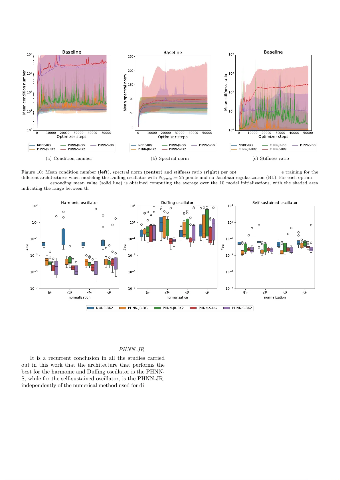
Con trolled oscillation mo deling using p ort-Hamiltonian neural net w orks M. Linares a, ∗ , G. Doras a , T. Hélie a , A. Ro ebel a a IRCAM, 1, place Igor-Str avinsky, 75004, Paris, F r anc e Abstract Learning dynamical systems through purely data-driven metho ds is c hallenging as they do not learn the underlying conserv ation laws that enable them to correctly generalize. Existing p ort-Hamiltonian neural net work methods hav e recen tly b een successfully applied for mo deling mechanical systems. Ho wev er, even though these methods are designed on p ow er-balance principles, they usually do not consider p o w er-preserving discretizations and often rely on Runge- Kutta numerical metho ds. In this w ork, we prop ose to use a second-order discrete gradien t method em b edded in the learning of dynamical systems with p ort-Hamiltonian neural net works. Numerical results are provided for three systems delib erately selected to span diﬀeren t ranges of dynamical b eha vior under control: a baseline harmonic oscillator with quadratic energy storage; a Duﬃng oscillator, with a non-quadratic Hamiltonian oﬀering amplitude-dep enden t eﬀects; and a self-sustained oscillator, which can stabilize in a controlled limit cycle through the incorp oration of a nonlinear dissipation. W e show how the use of this discrete gradient metho d outp erforms the p erformance of a Runge-Kutta metho d of the same order. Exp eriments are also carried out to compare tw o theoretically equiv alent p ort-Hamiltonian systems form ulations and to analyze the impact of regularizing the Jacobian of port-Hamiltonian neural net works during training. Keywor ds: ph ysics-informed machine learning, port-Hamiltonian neural netw orks, discrete gradient, Jacobian regularization 1. In tro duction Purely data-driv en metho ds for dynamical systems p ose sev eral c hallenges: the volume of useful data is gener- ally limited, they pro duce accurate-but-wrong predictions, they are not capable of dealing with uncertain ty and their predictions are not explainable nor interpretable [1]. A t the same time, it is natural to leverage the prior knowl- edge obtained through centuries of scientiﬁc study in the form of inductive bias [2] when designing predictive mod- els [3]. In this direction, a successful data-driven ph ysical mo del is one whose inductive bias b etter captures the true dynamics and is able to predict a correct outcome for data not observ ed during training. These inductiv e bias are incorp orated through soft and hard constraints [4]. Soft constrain ts add p enalt y terms to the training loss func- tion, discouraging violations of ph ysical la ws. This ap- proac h is widely applicable, but the mo del must balance adherence to the constrain ts against ﬁtting the observ ed data, without providing an y formal guarantee. The sem- inal Physics-Informe d Neur al Networks (PINNs) [5] is an example of soft-constraining the model. In con trast, hard constrain ts ensure strict compliance with sp eciﬁed physical ∗ Corresponding author Email addresses: maximino.linares@ircam.fr (M. Linares), guillaume.doras@ircam.fr (G. Doras), thomas.helie@ircam.fr (T. Hélie), axel.roebel@ircam.fr (A . Ro eb el) la ws by embedding them directly into the mo del’s struc- ture, indep enden tly of the a v ailable data. In this sense, hard constraints can b e used to incorp orate energy con- serv ation laws, symmetry , numerical metho ds for PDEs or K o opman theory [6]. Ho wev er, imp osing hard constraints reduces the space of p ossible solutions and generally limits the mo del’s expressiv eness. As a result, hard constraints are diﬃcult to apply in practice: incorrect assumptions ab out the ph ysical system can lead to o verly biased mod- els with a p oor generalization p erformance. In this pap er, w e consider dynamical systems whose state x is go verned b y the following ODE: d x dt := ˙ x = f ( x ) (1) and analyze ho w hard constrain ts based on energy con- serv ation and p ow er balance principles are incorp orated in to neural netw orks based on physic al ly c onsistent p ort- Hamiltonian systems formulations. By physic al ly c onsis- tent , w e refer, in this w ork, to the com bination of p o w er- balanced state-space mo dels with discrete gradient n umer- ical metho ds, which preserve the system’s energy during discretization. The central hypothesis is that enforcing this physical structure as a hard constraint impro ves in- terpretabilit y and generalization with resp ect to a v anilla NeuralODE. T o substantiate this claim, w e conduct a sys- tematic study on three con trolled oscillatory systems of increasing mo deling complexit y: a harmonic oscillator, a Duﬃng oscillator and a self-sustained oscillator. These systems are delib erately selected to include linear and non- linear Hamiltonian dynamics as well as nonlinear dissipa- tion mechanisms. The harmonic oscillator serves as the simplest baseline example with quadratic energy storage; the Duﬃng oscillator oﬀers nonlinearities in the Hamil- tonian, capturing amplitude-dependent eﬀects; and the self-sustained oscillator incorp orates a nonlinear dissipa- tion which can stabilize the system in a con trolled-limit cycle. The main con tributions of this pap er are • a comparison of tw o theoretically equiv alent port- Hamiltonian systems (PHS) form ulations: the semi- explicit PH-Diﬀeren tial-Algebraic-Equations (PH-DAE) and the input-state-output PHS with feedthrough; when they are implemen ted as p ort-Hamiltonian neu- ral net works (PHNNs). • a p erformance comparison b et ween the Gonzalez dis- crete gradien t metho d, which is a second-order energy- preserving numerical metho d, and a second-order ex- plicit Runge-Kutta metho d when used to discretize the PHNN mo del during learning. • an empirical study of the impact of regularizing the Jacobian of PHNN through t wo metho ds already ap- plied to NeuralODEs and a new one tackling the stiﬀ- ness of the learned ODE solutions. The rest of this pap er is organized as follows. Section 2 introduces the necessary preliminaries on dynamical sys- tems, p ort-Hamiltonian systems, n umerical metho ds, neu- ral ordinary diﬀerential equations, and p ort-Hamiltonian neural net works. Section 3 presents the port-Hamiltonian form ulations considered in this work, the enforced physical constrain ts, and the oscillatory examples used throughout the pap er. Section 4 fo cuses on p ort-Hamitonian neural net works, detailing how physical constrain ts are incorp o- rated into the learning pro cess, the comparison b etw een con tinuous- and discrete-time mo dels, and the Jacobian regularization in the port-Hamiltonian neural netw orks. Section 5 form ulates the k ey researc h questions addressed b y the exp erimen tal study . Section 6 reports and dis- cusses the results of the exp erimen ts. Finally , Section 7 concludes the pap er and outlines directions for future w ork. The co de is publicly av ailable: https://github. com/mlinaresv/ControlledOscillationPHNNs [will b e re- leased after pap er acceptance]. 2. Preliminaries 2.1. Dynamic al systems 2.1.1. Dynamic al system ODE Consider a dynamical system gov erned b y the following system of equations: ( ˙ x ( t ) = f ( x ( t ) , u ( t )) y ( t ) = h ( x ( t ) , u ( t )) (2) where x ( t ) ∈ R n x , u ( t ) ∈ R n u and y ( t ) ∈ R n y are re- ferred to as the state , input and output of the system, resp ectiv ely; and where f : D → R n x , h : D → R n y are C 1 functions with domain D ⊆ R n x × R n u . The system of equations (2) as a whole is referred to as state-sp ac e mo del [7]. In this work, w e consider autonomous systems (i.e. where u ( t ) is constant for all t ). Obtaining a solution for a given initial condition is often referred to as solving the initial value pr oblem (IVP) ˙ x ( t ) = f ( x ( t )) x (0) = x 0 . (3) In the following, we omit the explicit time dep endence of x ( t ) , y ( t ) and u ( t ) to simplify the notation, when there is no am biguity , and w e let J f ( x ) denote the Jac obian matrix of the function f of (3). 2.1.2. W el l-p ose d pr oblems The term wel l-p ose d w as introduced to refer to prob- lems where a) the solution exists, b) is unique, and c) dep ends contin uously on the initial conditions and param- eters [8]. A suﬃcient condition for an IVP to b e well-posed is that f is K -Lipschitz [9]. The sp e ctr al norm of a matrix A is deﬁned as: ∥ A ∥ 2 = max ∥ x ∥ 2 =1 ∥ Ax ∥ 2 = σ max ( A ) , (4) where σ max ( A ) is the largest singular value of A [10]. It is a standard result that if the follo wing condition holds: ∥ J f ( x ) ∥ 2 ≤ K < ∞ ∀ x ∈ D then f is K-Lipsc hitz [9] (see App endix A). In practice, controlling the well-posedness of the IVP reduces to enforcing an upper b ound on the sp ectral norm of the Jacobian of f . 2.1.3. W el l-c onditione d pr oblems The term wel l-c onditione d refers to problems seen as a function f where a small p erturbation of x yields only small changes in f ( x ) – the meaning of smal l depending 2 on the context [11]. This relationship can b e characterized b y the r elative c ondition numb er of f deﬁned as: κ f ( x ) = lim δ → 0 sup ∥ δ x ∥≤ δ  ∥ f ( x + δ x ) − f ( x ) ∥ 2 ∥ f ( x ) ∥ 2  ∥ δ x ∥ 2 ∥ x ∥ 2  , (5) where δ x and δ f are inﬁnitesimal. If f ∈ C 1 , this rewrites as: κ f ( x ) = ∥ J f ( x ) ∥ 2 ∥ f ( x ) ∥ 2 / ∥ x ∥ 2 . (6) for ∥ x ∥ 2  = 0 and its limit when ∥ x ∥ 2 → 0 . If κ f ( x ) is small (resp. large), the problem is said to b e wel l-c onditione d (resp. il l-c onditione d ). F or a linear system f ( x ) = Ax , the Jacobian of f b ecomes J f ( x ) = A , ∀ x . It is a standard result that the condition n umber can then b e b ounded s.t.: κ f ( x ) ≤ ∥ J f ( x ) ∥ 2 ∥ J − 1 f ( x ) ∥ 2 = σ max ( J f ( x )) σ min ( J f ( x )) (7) where σ max ( J f ( x )) , σ min ( J f ( x )) are the maximum and minim um singular v alues of J f ( x ) [11]. In the following, the upp er bound in (7) is denoted as κ ( J f ( x )) . In practice, controlling the w ell-conditioning of a linear problem f reduces to enforcing an upper b ound on its condition n umber. 2.1.4. Stiﬀ ODE systems The term stiﬀ refers to an initial v alue problem for whic h certain numerical methods require prohibitively small step sizes to main tain stability . This b ehavior can b e c har- acterized b y the stiﬀness r atio deﬁned as: ρ ( J f ) = max |R ( λ ( J f )) | min |R ( λ ( J f )) | , (8) where λ ( J f ) are the eigenvalues of the Jacobian matrix and R ( · ) : C → R is the real part operator [12]. Although it is rigorously only true for linear equations, a system with a large stiﬀness ratio is generally stiﬀ [12]. In practice, controlling the stiﬀness of an ODE system reduces to enforcing an upp er bound on its stiﬀness ratio. 2.2. Port-Hamiltonian systems In the Hamiltonian formalism [13], the mechanical state of S is represen ted by a vector x = [ q , p ] ⊤ ∈ R n x , where q , p ∈ R n x / 2 denote the generalized coordinates and con- jugate momen ta. The dynamics is go v erned through a scalar-v alued energy function H ( x ) known as Hamiltonian , and the time evolution of the system follows Hamilton’s equations: ˙ x = f ( x ) = S ∇ H ( x ) =  0 I n − I n 0  ∇ H ( x ) , (9) where S ∈ R n x × n x is the canonical symplectic matrix whic h imp oses the energy conserv ation principle. This formalism is restricted to conserv ative closed systems and do es not readily describ es dissipation or external control, whic h are common to many real-w orld systems. P ort-Hamiltonian formalism [14–16] generalizes Hamil- tonian mechanics to m ulti-physics op en systems b y ex- plicitly mo deling energy exchange with the environmen t through ports (inputs/outputs) and dissipation. In this w ork, the considered class of op en systems is represen ted in this formalism as a net work of: • ener gy storing c omp onents with state x and energy E := H ( x ) , with H p ositive deﬁnite and C 1 -regular, so the stored p o w er is P stored := ˙ E = ∇ H ( x ) ⊤ ˙ x , • dissip ative c omp onents , describ ed b y an eﬀort la w z ( w ) for a ﬂow v ariable w , where P diss := z ( w ) ⊤ w ; b y con v ention, the dissipated pow er is coun ted p osi- tiv ely , i.e. P diss ≥ 0 , with P diss = 0 for conserv ative comp onen ts, • external c omp onents are represen ted through p orts b y system inputs u and outputs y , with the conv en- tion that P ext := u ⊤ y is p ositiv e when received by these external comp onen ts. The coupling of in ternal ﬂo ws F and eﬀorts E gov erns the time ev olution of the system, expressed as:   ˙ x w y   | {z } := F = S   ∇ H ( x ) z ( w ) u   | {z } := E , (10) where S = − S T is sk ew-symmetric so that 0 = P stored | {z } ∇ H ( x ) T ˙ x + P diss | {z } z ( w ) T w + P ext |{z} u T y = ⟨E |F ⟩ (11) with ⟨E |F ⟩ = E T F . Indeed, E T F (14) = E T S E ( S = − S T ) = 0 (12) The passivit y of the system stems from the fact that P diss ≥ 0 , which imp oses that P stored = − P diss − P ext ≤ − P ext . As a consequence, P stored ≤ 0 (non-increasing in ternal energy) when external sources are oﬀ. This intrinsically physics- consisten t form ulation is highly general and can be ap- plied to a wide range of physical domains, including acous- tics, ﬂuid mec hanics, quantum physics and others [17–21] (see [16] for form ulations more general than (10)). 2.3. Numeric al metho ds F or a given IVP (3), a numeric al metho d approximates the solution without the need to analytically solve the ODE. A discr ete tr aje ctory T is deﬁned as the set { x n } n ∈ N 3 of consecutiv e states where x n := x ( nh ) , h = 1 /sr is the time step and sr the sampling rate. Given the initial state x 0 = x (0) , the applied control u and the ODE go verning x , a tra jectory T is obtained b y such n umerical metho d. If the gov erning equation is given by (10), the resulting T is said to b e a discr etization of a p ort-Hamiltonian system . In this work, we use numerical metho ds that belong to tw o diﬀeren t categories: 2.3.1. R unge-Kutta (RK) metho ds A w ell-known family of numerical metho ds is the Runge- Kutta metho ds [22]. Let b i , a i,j ( i, j = 1 , ..., s ) b e real n umbers and let c i = P s j =1 a ij . An s-stage Runge-Kutta metho d is giv en b y ( k i = f  t 0 + hc i , x n + h P s j =1 a i,j k j  , i = 1 , ..., s x n +1 = x n + h P s i =1 b i k i (13) where the weigh ts b i , a i,j are chosen to reach an accuracy order. In particular, the explicit midp oint metho d (RK2) x n +1 = x n + f  t n + h 2 , x n + h 2 f ( t n , x n )  (14) is a second-order explicit Runge-Kutta metho d. 2.3.2. Discr ete gr adient (DG) metho ds Ph ysical prop erties lik e energy-preserv ation are not in general resp ected when discretizing a p ort-Hamiltonian system using RK metho ds [23]. How ever, in Hamiltonian mec hanics there is a ric h theory of structure preserving in tegrators [22]. In particular, discrete gradient metho ds are a family of geometrical integrators that preserve the exact energy by construction [24]. A discr ete gr adient ∇ H : R n x × R n x → R n x is an approximation of the gra- dien t of a function H : R n x → R , satisfying the following t wo properties 1 : 1. ∇ H ( x , δ x ) T δ x = H ( x + δ x ) − H ( x ) 2. ∇ H ( x , 0 ) = ∇ H ( x ) where δ x = x ′ − x . In this w ork, we consider the Gonzalez discr ete gr adient method [25] (DG) ∇ mid H ( x , δ x ) = ∇ H  x + 1 2 δ x  + H ( x + δ x ) − H ( x ) − ∇ H ( x + 1 2 δ x ) T δ x δ x T δ x δ x . (15) Note that this metho d is, in general, a second-order inv erse- explicit in tegrator [26] that b ecomes linearly implicit when the Hamiltonian satisﬁes H ( x ) = 1 2 x T Qx . 1 In the literature, these two prop erties are usually written as 1. ∇ H ( x , x ′ ) T ( x ′ − x ) = H ( x ′ ) − H ( x ) 2. ∇ H ( x , x ) = ∇ H ( x ) . 2.4. Neur al ODEs and Jac obian r e gularization Neur al Diﬀer ential Or dinary Equations (NODEs) were in tro duced b y Chen et al. [27] to deﬁne the evolution of a system’s state using an ODE whose dynamics are mo deled b y a neural netw ork: d x ( t ) dt = f θ ( t, x ( t )) (16) where θ represents the parameters of the neural netw ork. The forw ard pass of a NODE is deﬁned as x ( t n +1 ) = x ( t n ) + Z t n +1 t n f θ ( t, x ( t )) dt (17) where in practice the in tegration is approximated by an y n umerical metho d. A well-documented challenge in the training of NODEs is the fact that the Jacobian of the learned dynamics f θ b e- comes p oorly conditioned as the training progresses. Sev- eral studies hav e underlined this phenomenon. F or in- stance, Dupont et al. [28] rep orted that when NODEs are o verﬁtted on the MNIST dataset [29], the resulting ﬂow ma y become so ill-conditioned that the numerical ODE solv er is forced to tak e time steps smaller than mac hine precision, leading to numerical underﬂow and an increase in the num b er of function ev aluations (NFE). Such patho- logical dynamics can also destabilize training and cause the loss to diverge. Motiv ated b y these observ ations, Finla y et al. [30] emphasized the imp ortance of explicitly con- straining the learned vector ﬁeld. They noted that, in the absence of such constraints, the learned dynamics may ex- hibit po or conditioning, which in turn degrades n umerical in tegration and degrades training performance. T o ad- dress this issue, they prop osed regularizing the Jacobian of f θ using its F rob enius norm. In this direction, Josias et al. [31] prop osed instead to regularize the Jacobian con- dition n umber, arguing that it reduced NFE without a signiﬁcan t loss in accuracy and controlling at the same time the Jacobian norm. F o cusing on Jacobian regular- ization enables a connection to sensitivity analysis found in neural netw ork literature, where also the sp ectral norm regularization has b een emplo y ed [32] [33]. 2.5. Port-Hamiltonian neur al networks In the con text of learning Hamiltonian ODEs, Grey- dan us et al. [34] introduced Hamiltonian Neur al Network (HNN), modifying the usual NODEs framew ork b y param- eterizing the Hamiltonian function of a giv en conserv ative ph ysical system. Once the Hamiltonian is parameterized, (9) is leveraged in the loss function. This work led to man y others trying to generalize the framew ork to learn more general ph ysical systems. F or example, Sosan ya et al. [35] generalized the approac h of HNN to non-conserv ative sys- tems using Helmholtz’s decomp osition theorem to param- eterize the dissipation p oten tial. Several w orks integrating p ort-Hamiltonian systems theory in to neural netw orks are 4 found in literature. Most of them implement the input- state-output represen tation 2 [16] ( ˙ x = ( J ( x ) − R ( x )) ∇ x H ( x ) + G ( x ) u y = G T ( x ) ∇ H ( x ) (18) for designing the computation graph of the dynamics. In this con text, Desai et al. [36] introduce the Port-Hamiltonian Neur al Network (PHNN) to learn damp ed and con trolled systems. Zhong et al. [37] use this formulation to mo del conserv ative systems with external control in tro ducing the Symple ctic ODE-Net (SymODEN). In another work, the same authors generalize the framework of SymODEN to learn also the dissipation [38]. Cheriﬁ et al. [39] prop ose a framework based on input-state-output data to learn p ort-Hamiltonian systems describ ed by (18). Roth et al. [40] introduce Stable Port-Hamiltonian Neur al Networks (sPHNN) to learn dynamical systems with a single equilib- rium under s tabilit y guarantees. A similar work to the one presen ted in this article, but based on pseudo-Hamiltonian formalism, is found in [4]. These approac hes learn the dy- namics through (18) and imp ose a priori knowledge, ei- ther on the expression of the Hamiltonian [37–41] or on the wa y dissipation aﬀects the system [4, 36, 39, 40]. As in an y other NODE framework, (18) is discretized, during or after the training, using a numerical metho d so that there is no preserv ation of the pow er balance and no guar- an tee of stability . Generally , this has been done either b y high-order RK metho ds [34–36, 39, 40], but also via symplectic integrators [41–45], although the impact on the accuracy of one or the other approach has not b een thor- oughly studied. T o the b est of our knowledge, the use of discrete gradients metho ds has not yet been describ ed in the PHNN literature. 3. P ort Hamiltonian Mo dels 3.1. Port-Hamiltonian formulations Let x ∈ X ⊂ R n x b e the state of S with an asso ciated Hamiltonian H : X → R and u , y ∈ R n u b e the input and output of the system, resp ectiv ely . W e consider three form ulations in this work: (i) Semi-explicit PH-Diﬀeren tial-Algebraic-Equations (PH- D AE):   ˙ x w y   | {z } ﬂows F i = S   ∇ H ( x ) z ( w ) u   | {z } eﬀorts E i , (19) where S = − S T ∈ R ( n x + n w + n u ) × ( n x + n w + n u ) and z ( w ) : R n w → R n w is the resistive structure of S . 2 In the literature, this equation adopts the conv ention that u T y = P ext is positive when given to the system by the exter- nal comp onen ts, so that P ext = − P ext and that ( u , y ) = ( u , − y ) or ( − u , y ) , contrary to conv entions used in (10) and all this pap er The skew-symmetry of S guarantees energy conser- v ation and the resistive prop erty of z ( w ) is giv en by z ( w ) T w ≥ 0 , which guaran tees passivity . (ii) Input-state-output PHS with feedthrough [46]:  ˙ x y  |{z} ﬂows F ii =  J − R ( x , u )   ∇ H ( x ) u  | {z } eﬀorts E ii , (20) where J and R ( x , u ) ∈ R ( n x + n u ) × ( n x + n u ) satisfy J = − J T and R = R T ⪰ 0 . The skew-symmetry of J accounts for conserv ativ e connections and the p ositiv e semi-deﬁniteness of R ( x , u ) guaran tees pas- sivit y . This formulation can be retriev ed from (i) in particular when S ww = 0 and S wx , S wu do not de- p end on w . It is also an extension of (18) for systems with direct feed-through. (iii) Sk ew-symmetric gradien t PH-DAE: If the function z ( w ) = ∂ w Z ( w ) is deriv ed from a p otential Z (often referred to as the Ra yleigh potential), the system (19) rewrites as the sk ew-gradient system [47]   ˙ x w y   | {z } ﬂows F iii = S ∇ F     x w u     | {z } eﬀorts E iii , (21) where S = − S T ∈ R ( n x + n w + n u ) × ( n x + n w + n u ) and F = H ( x ) + Z ( w ) + u T u 2 . Only the form ulations (i) and (ii) are considered in the exp erimen ts. The skew-symmetric gradient PH-D AE is presen ted as a generalization of the formulation used by Sosan ya et al. [35]. The PHS formulations (i-iii) are passive (see App endix B). 3.2. Physic al c onstr aints enfor c ement The general class of ph ysical systems considered in this w ork is such that the Hamiltonian H is C 1 -regular p ositive deﬁnite. In addition, we consider the sub class of Hamilto- nians of the form H ( x ) = 1 2 x T Q ( x ) x , (22) where Q ( x ) is a C 1 -regular symmetric p ositiv e deﬁnite ma- trix function. As already mentioned, The PHS form ula- tions (i)-(ii) satisfy t wo t yp es of constraints b y construc- tion: ( S (or J ) skew-symmetric (energy conserv ation) z ( w ) T w ≥ 0 , ∀ w (or R ⪰ 0) (passive la ws) (23) In the PH-DAE formulation, w e consider the sub class of dissipation function of the form: z ( w ) = Γ ( w ) w (24) 5 where Γ ( w ) ∈ R n w × n w is C 0 -regular p ositiv e semideﬁnite matrix function that admits a symmetric/sk ew-symmetric decomp osition Γ ( w ) = Γ skew ( w ) + Γ sy m ( w ) with Γ skew = 1 2 ( Γ − Γ T ) and Γ sy m = 1 2 ( Γ + Γ T ) ⪰ 0 . The resistiv e prop ert y is satisﬁed as ∀ w , z ( w ) T w = w T Γ( w ) T w = w T Γ sy m ( w ) T w Γ sym ⪰ 0 ≥ 0 (25) Note that the classes of systems describ ed b y equations (22) to (25) co ver a large sp ectrum of physical systems and remain fairly general. 3.3. R ep ar ameterization of c onstr aints W e no w reparameterize the matrix constrain ts using the follo wing prop erties: • an y symmetric p ositiv e semideﬁnite (resp. deﬁnite) matrix M sy m can b e written in the form M sy m = L T L where L is a lo wer triangular matrix with pos- itiv e (resp. strictly p ositiv e) diagonal co eﬃcients (Cholesky factorization [48]), • an y skew-symmetric matrix M skew can b e written in the form M skew = K − K T where K is a strictly lo wer triangular matrix. Then, the ph ysical constraints (23) are naturally satis- ﬁed considering the follo wing reparametrizations: Q ( x ) = L T Q ( x ) L Q ( x ) (26) Γ ( w ) = L T Γ ( w ) L Γ ( w ) + K Γ ( w ) − K T Γ ( w ) or (27) R ( x , u ) = L T R ( x , u ) L R ( x , u ) (28) where L Q,R, Γ , resp. K Γ , are low er, resp. strictly low er, triangular matrices. 3.4. Oscil latory physic al examples Three oscillating systems that satisfy (22)-(24) are con- sidered: • the harmonic oscillator, which is quadratic in energy , with a linear dissipation; • the Duﬃng oscillator, which is non-quadratic in en- ergy , with a linear dissipation; • a self-sustained oscillator, which is quadratic in en- ergy , with a nonlinear dissipation. This last ph ysical system is of particular dynamical in ter- est as it is designed to self-oscillate when combined with an adapted constan t input, leading to a stable limit cycle [49]. T able 1 shows the diﬀerent port-Hamiltonian structural el- emen ts for each of these systems. 4. P ort-Hamiltonian neural netw orks 4.1. Port-Hamiltonian neur al network mo dels A p ort-Hamiltonian neural netw ork (PHNN) parame- terizes the righ t-hand side of (19)-(20), mo deling the Hamil- tonian and the dissipative terms with tw o distinct neural net works. In this work, we assume that the interconnec- tion matrices J and S , are given a priori. The Hamiltonian function is parameterized identically for eac h formulation b y a neural netw ork H θ H ( x ) , and its gradien t is derived b y auto-diﬀerentiation as prop osed in the seminal HNN [34]. The implementation of the dissipativ e term dep ends on the form ulation considered (i or ii), whic h yields tw o diﬀeren t PHNN architectures: (i) PHNN-S mo dels (19), where the dissipation function z ( w ) : R n w → R n w is parameterized by a neural net- w ork z θ z ( w ) , implemen ting the dynamic function: f θ ( x , u ) = f S θ ( x , u ) = S   ∇ H θ H ( x ) z θ z ( w ) u   (29) (ii) PHNN-JR models (20), where the co eﬃcien ts of the dissipation matrix R ( x , u ) are parameterized by the outputs a neural netw ork R θ R ( x , u ) , implementing the dynamic function: f θ ( x , u ) = f J R θ ( x , u ) = ( J − R θ R ( x , u ))  ∇ H θ H ( x ) u  (30) Figure 1 shows the architecture of the t wo diﬀeren t PHNN mo dels according to eac h of the PHS formulations. 4.2. Physic al c onstr aints enfor c ement in neur al networks A ccording to Section 3.2, the PHS mo del is passive if the Hamiltonian and the dissipative terms take the form of (26) and (27) or (28). The non-zero coeﬃcients of a n × n lo w er (resp. strictly lo wer) triangular matrix can be parameterized b y the n ( n + 1) / 2 (resp. n ( n − 1) / 2 ) outputs of a neural netw ork L θ L (resp. K θ K ), implementing the functions:        H θ H ( x ) = 1 2 x T L T θ L H ( x ) L θ L H ( x ) x z θ z ( w ) =  L T θ L z ( w ) L θ L z ( w ) + K θ K z ( w ) − K T θ K z ( w )  w R θ R ( x , u ) = L T θ L R ( x , u ) L T θ L R ( x , u ) (31) This parametrization is widely used in the literature [37, 39, 40, 50, 51]. T able 2 shows the ﬁxed and learned ob jects for the port-Hamiltonian netw orks based on formulations (i) and (ii). 6 System Harmonic oscillator Duﬃng oscillator Self-sustained oscillator (linear) (nonlinear) (nonlinear) x =  q p  u q : cen tered p osition (elongation) [m] p : momentum [Kg.m.s − 1 ] u = f : force (applied or exterior) [N] H ( x ) p 2 2 m + k q 2 2 p 2 2 m + k 1 q 2 2 + k 3 q 4 4 p 2 2 m + k q 2 2 J J =   0 1 0 − 1 0 − 1 0 1 0   J =   0 − 1 0 1 0 0 0 0 0   R R = α   0 0 0 0 1 0 0 0 0   with α > 0 [N /ms − 1 ] R = Γ( w )   1 0 1 0 0 0 1 0 1   with Γ( w ) > 0 [ m/s N] S S =     0 1 0 0 − 1 0 − 1 − 1 0 1 0 0 0 1 0 0     S =     0 − 1 1 0 1 0 0 0 − 1 0 0 − 1 0 0 1 0     Γ( w ) α aw 2 + bw + c z ( w ) z ( w ) = α w z ( w ) = aw 3 + bw 2 + cw Z ( w ) Z ( w ) = αw 2 2 Z ( w ) = aw 4 4 + bw 3 3 + cw 2 2 J f ( x )  0 1 m − k − α m   0 1 m − k 1 − 3 k 3 q 2 − α m   − Γ ′ ( w ) kq − Γ( w ) k − 1 m k 0  ∥ J f ( x ) ∥ 2 p λ max (( J f ( x )) T J f ( x )) (see the exact details on the App endix C) κ ( J f ( x )) σ max ( J f ( x )) σ min ( J f ( x )) = q λ max (( J f ( x )) T J f ( x )) λ min (( J f ( x )) T J f ( x )) (see the exact details on the App endix C) ρ ( J f ( x )) 1 , if the system is underdamp ed T able 1: Diﬀeren t p ort-Hamiltonian structural elements, Jacobian matrices and related quan tities for the considered oscillators. (a) Arc hitecture of PHNN-S (b) Arc hitecture of PHNN-JR Figure 1: Architecture of the tw o PHNN mo dels considered in this w ork. White b o xes with orange contour denote ﬁxed algebraic op erations whereas orange boxes indicate the trainable parameters. 4.3. Continuous- vs. discr ete-time mo dels A c ontinuous mo del f θ ( x t , u t ) represents the ﬁeld ˙ x t . During training, it learns an estimate of ˙ x t b y minimizing the loss L c = ∥ ˙ x t − f θ ( x t , u t ) ∥ 2 2 (32) During inference, it is integrated as the right-hand side of the ODE using a n umerical metho d. A discr ete mo del g θ,h ( x n , u n ) represen ts the next state x n +1 . During training, it learns an estimate of x n +1 b y minimizing the loss L d =     x n +1 − g θ,h ( x n , u n ) h     1 (33) via bac kpropagation through a diﬀerentiable numerical ODE solv er using a discretization step h . W e introduce (33) inspired by Zhu et al. [52], as it was shown to hav e the- oretical guarantees for NeuralODEs using explicit Runge Kutta methods (see [52], Theorem 3.1). During inference, the discrete mo del is applied autoregressively to predict future states. Examples of discrete PHNN model learning framew ork can b e found in literature [37, 38, 41, 53]. 7 Ob jects F ormulation (i)     ˙ x y     = ( J − R ( x , u ))     ∇ H ( x ) u     (ii)         ˙ x w y         = S         ∇ H ( x ) z ( w ) u         H ( x ) H θ H ( x ) = 1 2 x T L θ L H ( x ) T L θ L H ( x ) x Dissipation R θ R ( w ) = L θ L R ( x , u ) T L θ L R ( x , u ) z θ z ( w ) = Γ θ Γ ( w ) w Γ θ Γ ( w ) = ( L T θ L z ( w ) L θ L z ( w )) + ( K θ K z ( w ) − K T θ K z ( w )) In terconnection matrix J ∈ R ( n x + n u ) × ( n x + n u ) S ∈ R ( n x + n w + n u ) × ( n x + n w + n u ) T able 2: Fixed and learned ob jects for the diﬀerent p ort-Hamiltonian networks based on formulations (i) and (ii). Numerical Schema T rain Inference Figure 2: T raining and inference diagram for the continuous mo dels f θ . Numerical Schema T rain Inference Figure 3: T raining and inference diagram for the discrete mo dels g θ . As it can b e seen on Figures 2 and 3, the neural net- w ork parameterizing the con tinuous- and the discrete-time mo dels is the same. How ever, the ODE solver is used at diﬀeren t phases: during training and inference for discrete- time mo del, but only during inference for con tin uous-time mo del. In this work, we fo cus on discrete mo dels, where the tw o diﬀerent ODE solver schemes compared are sho wn in T able 3. This decision is based on the fact that in prac- tice it is generally imp ossible to ha v e access to state deriv a- tiv es ˙ x t . F ollo wing (33), training discrete mo dels do es not require state deriv ative measurements and relies only on state measurements. Nevertheless, their performance dur- ing inference is limited to using the same discretization step h as during training. 4.4. Jac obian r e gularization on PHNN Let J f θ ( x , u ) denote the Jacobian of a PHNN, where f θ ( x , u ) corresp onds to (29)-(30). Ideally , we would like Accuracy order Name Characteristic Pow er-balance 2 Explicit midp oin t (RK2) Explicit × 2 Discrete gradient (DG) Inv erse-explicit ✓ T able 3: A ccuracy order, name, c haracteristic and whether pow er- balance is respected for the chosen numerical schema. f θ ( x , u ) not only to b e ph ysically-consistent, which is al- ready structurally guaran teed in the PHNNs, but also nu- meric al ly smo oth . This means that, among the diﬀer- en t ph ysically-consistent solutions learned by our mo d- els, those that are ill-p osed, ill-conditioned or highly stiﬀ should b e p enalized through some kind of Jacobian reg- ularization, as prop osed in the NeuralODE literature [28, 30, 31]. F ollo wing this approac h, w e soft-constrain t the training loss L d to av oid non-desirable numerical b eha v- iors in the PHNNs. W e exp eriment with regularizing the sp ectral norm ∥ J f θ ∥ 2 , 8 the condition num b er κ ( J f θ ) or the stiﬀness ratio ρ ( J f θ ) as deﬁned in Section 2.1. Penalizing higher sp ectral norm v alues promotes solutions with a low er Lipschitz constan t whereas doing so with condition num b er rew ards well- conditioned solutions. The rationale for introducing ρ ( J f θ ) as a new regularization term stems from the observ ation that ill-conditioned Jacobians, often asso ciated with a high NFE in adaptive n umerical metho ds, are characteristic of stiﬀ ODE systems. Th us, p enalizing large v alues of ρ ( J f θ ) discourages the training pro cedure from con verging to- w ard stiﬀ dynamics, thereby promoting indirectly b etter- conditioned ODE solutions. During the training, these regularization quan tities are obtained after ev aluating the Jacobian at the input data from a given batch, making the same assumption as in [31]: that r e gularizing dynamics at the input data c an le ad to r e gularize d dynamics acr oss the entir e solution sp ac e . The follo wing loss functions with Jacobian regularization terms are in tro duced: L C N = L d + λ C N ∥ κ ( J f θ ( x , u )) ∥ 2 2 (34) L S N = L d + λ S N ∥ J f θ ( x , u ) ∥ 2 (35) L S R = L d + λ S R ∥ ρ ( J f θ ( x , u )) − 1 ∥ 2 2 (36) W e set λ S N = 10 − 6 , λ C N = 10 − 6 and λ S R = 10 − 4 in later exp erimen ts, and, as in [31], we add 10 − 6 to the denominator of κ ( J f θ ) and ρ ( J f θ ) to av oid underﬂow in the early stages of training. 5. Exp erimen ts 5.1. Our questions Giv en a discrete tra jectory T and its initial state x 0 , the ob jective of this work is to design PHNN mo dels capa- ble of accurately generating a tra jectory ˜ T = { ˜ x n } n ∈ N + , with ˜ x 0 = x 0 , that appro ximates T as closely as possible. Eac h of the PHNN mo dels presen ted in this w ork can b e c haracterized by the: 1. PHS form ulation: PHNN-S or PHNN-JR. 2. T yp e of mo del: Contin uous or discrete. 3. Numerical metho d: RK2 or DG (see T able 3). 4. Num b er of trainable parameters: 800, 2k or 10k. 5. Num b er of training p oin ts: 25, 100 or 400. 6. Loss function: L d , L S N , L C N or L S R . W e set a b aseline NODE [27] mo del and conduct several exp erimen ts to compare its p erformance to th e prop osed familiy of PHNNs mo dels. Study I : Impact of the num b er of training points . The ﬁrst study fo cuses on how the diﬀerent PHNN arc hi- tectures compare at inference stage with diﬀerent n umer- ical metho ds for the systems in T able 1. F or this study , exp erimen ts are carried out for 25, 100 and 400 training p oin ts and the smallest num b er of training parameters is considered ( ≈ 800 ). Study II : Impact of the num b er of trainable pa- rameters . The second study uses the same combination of PHNN architectures and numerical metho ds but, oppo- site to Study I, the n umber of training p oin ts is ﬁxed to 25 and the num b er of training parameters v aries b et w een smal l ( ≈ 800 ), me dium ( ≈ 4 k ) and lar ge ( ≈ 20 k ). T ables E.8-E.10 in App endix D detail the design choices of the neural netw ork comp onen ts for eac h mo del. In each case, the criteria is to hav e a similar num b er of parameters for eac h formulation, whic h enables a fair comparison b et ween them. Study III : Impact of the Jacobian regularizations . The third study fo cuses on ho w the diﬀerent Jacobian regularizations in (34)-(36) inﬂuence the inference p erfor- mance of the mo dels. In this case, the same com bination of PHNN architectures, numerical metho ds, training pa- rameters and training p oin ts as in Study I is considered. 5.2. Implementation details T able 4 shows the parameters considered for the gen- eration of tra jectories for each physical system as w ell as the training and inference parameters considered for the neural net work exp erimen ts, whereas Figure 4 shows the distribution of the training and test p oin ts as well as tw o complete test tra jectories for each oscillatory system. Generation of synthetic data . The dataset T con- sists of N traj = 12500 tra jectories. Each tra jectory is generated syn thetically according to the following criteria: i Initial condition : W e ﬁx E min , E max , and we sam- ple an initial condition x 0 suc h that H ( x 0 ) ∈ I E 0 = [ E min , E max ] (37) with E min , E max ∈ R + (see T able 4 for n umerical v alues). ii Con trol : F or the harmonic and Duﬃng oscillators, external con trol is applied as a constant force u so that H ( x ∗ ) ∈ I E eq = [ E min eq , E max eq ] (38) where x ∗ is the equilibrium point of the system. In con trol theory , this is usually referred to as p otential ener gy shaping [54]. F or the self-sustained oscillator, the external constan t con trol u is applied so that the system stabilizes in a limit cycle around x ∗ (see T able 4 for numerical v alues). F urther details about the sampling of the initial condi- tions and the con trol design can be found in App endix E. As for the intrinsic parameters of each system, they are c hosen to satisfy that the natural frequency f 0 is 1 H z . F or the harmonic and Duﬃng oscillator, a linear dissipa- tion function z ( w ) = cw is considered. In this case, c is c hosen so that the damp ed harmonic oscillator has dissi- pated 99% of its energy in D = 5 T 0 = 5 s , where T 0 = 1 /f 0 9 System Harmonic Oscillator Duﬃng Oscillator Self-sustained oscillator In trinsic parameters ( m, k ) ( m, k 1 , k 3 ) ( m, k ) f 0 [Hz] 1 H z m [kg] 0 . 16 1 /k , 1 /k 1 [ N /m ] 0 . 16 k 3 [ N /m 3 ] - 100 k 1 - z ( w ) 0 . 9 w [N] 1 . 3 w 3 − 4 w 2 + 3 w [ m/s ] Constan t control u [N] Suc h that the equilibrium p oin t energy lies in I E 0 Suc h that system reaches a limit cycle I E 0 , I E eq [J] [0 . 1 , 1] sr g en [Hz] 400 f 0 Generation n umerical metho d Gonzalez discrete gradien t (15) α 0 . 31 β 5 D train [s] αT 0 D inf er [s] β T 0 sr train , sr inf er [Hz] 100 f 0 N train [25 , 100 , 400] Batc h size 64 N ev al 2500 N inf er 100 T able 4: Implemen tation hyperparameters for the diﬀerent exp eriments. 1.00 0.75 0.50 0.25 0.00 0.25 0.50 0.75 1.00 p 1.00 0.75 0.50 0.25 0.00 0.25 0.50 0.75 1.00 q T raining points T est trajectories T est initial points I s o e n e r g y l i n e s E 0 (a) Harmonic oscillator 1.00 0.75 0.50 0.25 0.00 0.25 0.50 0.75 1.00 p 1.00 0.75 0.50 0.25 0.00 0.25 0.50 0.75 1.00 q T raining points T est trajectories T est initial points I s o e n e r g y l i n e s E 0 (b) Duﬃng oscillator 1.00 0.75 0.50 0.25 0.00 0.25 0.50 0.75 1.00 p 1.00 0.75 0.50 0.25 0.00 0.25 0.50 0.75 1.00 q T raining points T est trajectories T est initial points I s o e n e r g y l i n e s E 0 (c) Self-sustained oscillator Figure 4: T raining p oin ts, test initial p oin ts and tw o complete test tra jectories for each of the three oscillatory systems. Note that in the case of the harmonic and Duﬃng oscillator, the applied con trol shifted the equilibrium p oin t from ( p, q ) = (0 , 0) whereas in the case of the self-sustained oscillator, it stabilizes the tra jectories in a limit cycle. is the natural p erio d. The same v alue of c is considered for the Duﬃng oscillator. As for the self-sustained os- cillator, the considered nonlinear dissipation function is z ( w ) = 1 . 3 w 3 − 4 w 2 + 3 w . In each physical system, the n umerical scheme considered for the generation of the tra- jectories is the Gonzalez discr ete gr adient (15) for a dura- tion D and a sampling rate sr g en = 400 f 0 . T raining details . Let D train = αT 0 and sr train = γ f 0 < sr g en b e the training time and data sampling rate, resp ectiv ely , where α and γ are hyperparameters. F or eac h system, w e consider α such that the harmonic os- cillator has dissipated 25% of its initial energy in the ab- sence of con trol and γ = 100 . The set of training tra jecto- ries T train is built considering N train tra jectories from T up until a duration T train sub-sampled at sr train . Once T train is created, one point ξ i train = (( x i n , u i n ) , x i n +1 ) is uniformly sampled from eac h tra jectory τ i train ∈ T train (see Figure 5 for a graphical description). The set of p oin ts ξ train = { ξ i train } i =1 ,...,N train constitutes the train- ing dataset. Note that training on a set of isolated p oin ts sampled at random from complete tra jectories is closer to exp erimen tal conditions than training on a set of complete tra jectories that might be more diﬃcult to measure accu- 10 D t r a i n D i n f e r Figure 5: Sc hematic sampling and dataset construction pro cedure. A tra jectory generated at sampling frequency sr gen ov er a duration D = D inf er = β T 0 is shown as white dot markers. F rom this tra jectory , a training p oint, highlighted with a green star marker, is uniformly sampled from a subset of samples, shown as black dot markers, ob tained at frequency sr train and restricted to t ≤ αT 0 . The training horizon D train and the inference horizon D inf er are indicated b y arrows, with the vertical dashed line marking the end of the training interv al. rately in practice. It also probably adds complexit y for the model, as isolated p oin ts are not ob viously correlated. Exp erimen ts are carried out for N train ∈ [25 , 100 , 400] . Af- ter each training ep o c h, mo dels are v alidated on another dataset ξ ev al , which is constructed as ξ train but for 2500 tra jectories. F or each of the datasets, exp erimen ts are car- ried out for 10 runs with diﬀerent mo del initializations us- ing the A dam optimizer [55] with a batch size 64 for 50 k optimizer steps with a learning rate of 10 − 3 . Inference details . The inference dataset T inf er is constructed taking a subset of N inf er = 100 tra jectories from T for a duration D inf er = β T 0 and a sampling rate sr inf er = sr train . Note that β ≫ α , i.e. the mo del has to generate in inference longer sequences that it has b een trained for. The p erformance of the mo del is then assessed generat- ing autoregressiv ely a tra jectory ˜ τ from eac h of the initial conditions of the tra jectories in T inf er and comparing it with the reference tra jectory τ . F or eac h mo del initializa- tion, w e compute the Mean Squared Error (MSE) b etw een the reference and predicted tra jectories: L traj = 1 N inf · T inf · f inf N inf X i =1 ∥ τ i − ˜ τ i ∥ 2 (39) 6. Results and discussions 6.1. Imp act of the numb er of tr aining p oints Figure 6 shows the inference error (see T able F.11 in the App endix F for the detailed n umerical v alues) for the diﬀeren t models across the three v alues of N train when learning the three con trolled oscillatory systems with small mo del size. As exp ected, increasing the num b er of p oin ts decreases the error for all systems and architectures, ex- cept for when we train the PHNN-S model on the self- sustained oscillator where the performance seems to be fairly constan t. The NODE architecture is consisten tly outp erformed by one of the ph ysically constrained mo d- els. Regarding the diﬀerences b etw een the tw o numerical metho ds, the discrete gradient outp erforms the RK2 in the lo w-data regime for the harmonic oscillator, and for every n umber of training p oints in the case of the nonlinear os- cillators. F or the Duﬃng oscillator, all p erformance errors sho w a high dispersion (as sho wn by large IQR) in the lo w-data regime, reﬂecting the model sensitivity to w eight initialization when very few training p oints are av ailable. Finally , whereas the PHNN-S mo del achiev es the lo w est p erformance error for the harmonic and Duﬃng oscillator, it is not the case for the self-sustained oscillator, where it is outperformed by the PHNN-JR and the NODE. Figure 7 compares the NODE with the b est PHNN architecture for each oscillator when discretizing a tra jectory starting on an initial condition x 0 suc h that H ( x 0 ) = 0 . 5 J . 6.2. Imp act of the numb er of tr ainable p ar ameters Figure 8 shows the inference error (see T able F.12 in the App endix F for the detailed n umerical v alues) for the diﬀeren t mo dels across the three regimes (small, medium, large) of trainable parameters when learning the three con- trolled oscillatory systems with N train = 25 . In this case, increasing the num b er of trainable parameters increases the error in general for all the systems and architectures. This can b e explained b y the fact that there are not enough 11 25 100 400 n_points 1 0 7 1 0 6 1 0 5 1 0 4 1 0 3 1 0 2 1 0 1 1 0 0 1 0 1 t r a j Har monic oscillator 25 100 400 n_points 1 0 7 1 0 6 1 0 5 1 0 4 1 0 3 1 0 2 1 0 1 1 0 0 1 0 1 t r a j Duffing oscillator 25 100 400 n_points 1 0 7 1 0 6 1 0 5 1 0 4 1 0 3 1 0 2 1 0 1 1 0 0 1 0 1 t r a j Self -sustained oscillator NODE-RK2 PHNN- JR -DG PHNN- JR -RK2 PHNN-S-DG PHNN-S-RK2 Figure 6: Bo xplot of the inference errors for the three diﬀerent oscillators and varying num b ers of training p oints (small models). F rom left to right: harmonic, Duﬃng and self-sustained oscillators. 0.4 0.2 0.0 0.2 0.4 p 0.4 0.2 0.0 0.2 0.4 q Gr ound truth NODE-RK2 PHNN-S-DG PHNN-S-RK2 (a) Harmonic oscillator 0.4 0.2 0.0 0.2 0.4 p 0.4 0.2 0.0 0.2 0.4 q Gr ound truth NODE-RK2 PHNN-S-DG PHNN-S-RK2 (b) Duﬃng oscillator 0.4 0.2 0.0 0.2 0.4 p 0.4 0.2 0.0 0.2 0.4 q Gr ound truth NODE-RK2 PHNN- JR -DG PHNN- JR -RK2 (c) Self-sustained oscillator Figure 7: Comparison of the learned tra jectory discretizations for each oscillatory system starting on x 0 such that H ( x 0 ) = 0 . 5 J . ( Left ) NODE and PHNN-S mo dels trained on N train = 25 from the harmonic oscillator. ( Cen ter ) NODE and PHNN-S mo dels trained on N train = 100 from the Duﬃng oscillator. ( Right ) NODE and PHNN-JR mo dels trained on N train = 25 from the self-sustained oscillator. F or the harmonic and Duﬃng oscillator, the tra jectory is obtained with u = 0 ; and for the self-sustained, with u such that the system stabilizes in a limit cycle. training samples to ﬁt larger mo dels and, thus, medium and large size mo dels directly ov erﬁt and are not able to generalize correctly . The NODE is again consistently outp erformed by one of the ph ysically constrained mo d- els. Regarding the impact of using the diﬀeren t n umerical metho ds, the discrete gradient only outperforms the RK2 when training small mo dels. Interestingly , increasing the n umber of trainable parameters has a p ositive eﬀect on the disp ersion of the results for the Duﬃng oscillator, as w e observ e ho w the IQR is reduced with resp ect to the small size setting. Figure 9 shows how the tra jectory dis- cretization from the b est PHNN arc hitecture for eac h os- cillator changes with resp ect to the num b er of trainable parameters starting on an initial condition x 0 suc h that H ( x 0 ) = 0 . 5 J . 6.3. Imp act of the Jac obian r e gularizations Regularizing the Jacobian of the PHNN models is mo- tiv ated by the p otential correlation existing b etw een the inference disp ersion and a high condition num b er, sp ec- tral norm or stiﬀness ratio mean v alue at the end of the training. As w e observ e in Figure 10, the mo dels with the highest mean condition num b er, sp ectral norm and stiﬀness ratio when mo deling the Duﬃng oscill ator with N train = 25 , i.e. PHNN-S-RK2 and PHNN-S-DG, are precisely the ones with a higher IQR v alue (see Figure 6 and T able F.11 in App endix F). F urthermore, their stiﬀ- ness ratio is higher than 1, meaning that these mo dels are 12 small_size medium_size lar ge_size model_size 1 0 7 1 0 6 1 0 5 1 0 4 1 0 3 1 0 2 1 0 1 1 0 0 1 0 1 t r a j Har monic oscillator small_size medium_size lar ge_size model_size 1 0 7 1 0 6 1 0 5 1 0 4 1 0 3 1 0 2 1 0 1 1 0 0 1 0 1 t r a j Duffing oscillator small_size medium_size lar ge_size model_size 1 0 7 1 0 6 1 0 5 1 0 4 1 0 3 1 0 2 1 0 1 1 0 0 1 0 1 t r a j Self -sustained oscillator NODE-RK2 PHNN- JR -DG PHNN- JR -RK2 PHNN-S-DG PHNN-S-RK2 Figure 8: Boxplot of the inference errors for the three diﬀerent oscillators and model sizes ( N train = 25 ). F rom left to right: harmonic, Duﬃng and self-sustained oscillators. 0.6 0.4 0.2 0.0 0.2 0.4 0.6 p 0.6 0.4 0.2 0.0 0.2 0.4 0.6 q Gr ound truth PHNN-S-small PHNN-S-medium PHNN-S-lar ge (a) Harmonic oscillator 0.6 0.4 0.2 0.0 0.2 0.4 0.6 p 0.6 0.4 0.2 0.0 0.2 0.4 0.6 q Gr ound truth PHNN-S-small PHNN-S-medium PHNN-S-lar ge (b) Duﬃng oscillator 0.4 0.2 0.0 0.2 0.4 p 0.4 0.2 0.0 0.2 0.4 q Gr ound truth PHNN- JR -small PHNN- JR -medium PHNN- JR -lar ge (c) Self-sustained oscillator Figure 9: Comparison of the learned tra jectory discretizations b y the discrete gradient for eac h oscillatory system starting on x 0 such that H ( x 0 ) = 0 . 75 J . ( Left ) PHNN-S mo dels trained on N train = 25 from the harmonic oscillator. ( Center ) PHNN-S models trained on N train = 25 from the Duﬃng oscillator. ( Right ) PHNN-JR models trained on N train = 25 from the self-sustained oscillator. F or the harmonic and Duﬃng oscillator, the tra jectory is obtained with u = 0 ; and for the self-sustained, with u such that the system stabilizes in a limit cycle. learning a representation that is stiﬀer than the original system from which we generate the data. Exp eriments are, th us, carried out to test whether controlling the numerical b eha vior through any of the prop osed Jacobian regulariza- tions lo wers the inference error and/or dispersion. Figure 11 sho ws the inference error (see T able F.13 in the App endix F for the detailed numerical v alues) when learning the three oscillatory systems under the diﬀer- en t Jacobian regularizations (34)-(36) with diﬀeren t small mo dels and N train = 25 . BL refers to the baseline (i.e. no Jacobian regularization); CN, to the condition n umber reg- ularization (34); SN, to the sp ectral norm regularization (35); and SR, to the stiﬀness ratio regularization (36). In general, Jacobian regularization do es not improv e the re- sults for those systems in which the mo del p erformances w ere already go od (harmonic and self-sustained oscillator). Ho wev er, CN-regularization considerably improv es the re- sults for the Duﬃng oscillator, where the disp ersion was high. In terestingly , controlling the stiﬀness ratio tow ards the ground truth system v alue is not directly associated with an improv emen t in the accuracy nor the disp ersion: the stiﬀness ratio v alues after SR-regularization are closer to 1 (see Figure 12) but the inference error or the disp er- sion is not alw ays reduced. 13 0 10000 20000 30000 40000 50000 Optimizer steps 1 0 0 1 0 1 1 0 2 1 0 3 1 0 4 Mean condition number Baseline NODE-RK2 PHNN- JR -RK2 PHNN- JR -DG PHNN-S-RK2 PHNN-S-DG (a) Condition n umber 0 10000 20000 30000 40000 50000 Optimizer steps 0 50 100 150 200 250 Mean spectral nor m Baseline NODE-RK2 PHNN- JR -RK2 PHNN- JR -DG PHNN-S-RK2 PHNN-S-DG (b) Spectral norm 0 10000 20000 30000 40000 50000 Optimizer steps 1 0 0 1 0 1 1 0 2 1 0 3 1 0 4 Mean stiffness ratio Baseline NODE-RK2 PHNN- JR -RK2 PHNN- JR -DG PHNN-S-RK2 PHNN-S-DG (c) Stiﬀness ratio Figure 10: Mean condition number ( left ), sp ectral norm ( cen ter ) and stiﬀness ratio ( righ t ) per optimizer step during the training for the diﬀerent architectures when mo deling the Duﬃng oscillator with N train = 25 p oints and no Jacobian regularization (BL). F or each optimizer step, the corresponding mean v alue (solid line) is obtained computing the av erage ov er the 10 mo del initializations, with the shaded area indicating the range b etw een the minimum and maximum v alues. BL CN SN SR nor malization 1 0 7 1 0 5 1 0 3 1 0 1 1 0 1 1 0 3 t r a j Har monic oscillator BL CN SN SR nor malization 1 0 7 1 0 5 1 0 3 1 0 1 1 0 1 1 0 3 t r a j Duffing oscillator BL CN SN SR nor malization 1 0 7 1 0 5 1 0 3 1 0 1 1 0 1 1 0 3 t r a j Self -sustained oscillator NODE-RK2 PHNN- JR -DG PHNN- JR -RK2 PHNN-S-DG PHNN-S-RK2 Figure 11: Bo xplot of the inference errors for the three diﬀerent oscillators and normalizations ( N train = 25 and small num b er of parameters). Notation: BL refers to the baseline (i.e. no Jacobian regularization); CN, to the condition num b er regularization (34); SN, to the spectral norm regularization (35); and SR, to the stiﬀness ratio regularization (36). F rom left to right: harmonic, Duﬃng and self-sustained oscillators. 6.4. Diﬀer enc es b etwe en PHNN-S and PHNN-JR It is a recurren t conclusion in all the studies carried out in this work that the architecture that p erforms the b est for the harmonic and Duﬃng oscillator is the PHNN- S, while for the self-sustained oscillator, is the PHNN-JR, indep enden tly of the n umerical metho d used for discretiza- tion. W e hypothesize that this could b e due to whether the dissipation of the system is nonlinear or not, implying that PHNN-S has diﬃculty learning the system’s dynam- ics in the presence of nonlinear dissipation, which is the case for the self-sustained oscillator. 7. Conclusion Con tributions . In this w ork, w e hav e addressed the problem of designing physic al ly c onsistent neural netw ork mo dels based on PHS form ulations and energy-preserving n umerical metho ds. The main contributions of this study include a comparison of tw o theoretically equiv alen t PHS form ulations: the PH-DAE and the input-state-output PHS with feedthrough, when implemented as PHNNs; a p erfor- mance comparison b et w een a second-order energy-preserving n umerical metho d and a Runge-Kutta metho d of the same order; and a empirical study of the impact of regularizing the Jacobian of PHNN through tw o metho ds already ap- 14 0 10000 20000 30000 40000 50000 Optimizer steps 1 0 0 1 0 1 1 0 2 1 0 3 1 0 4 Mean condition number CN-r egularization NODE-RK2 PHNN- JR -RK2 PHNN- JR -DG PHNN-S-RK2 PHNN-S-DG (a) Condition n umber 0 10000 20000 30000 40000 50000 Optimizer steps 0 50 100 150 200 250 300 350 Mean spectral nor m SN-r egularization NODE-RK2 PHNN- JR -RK2 PHNN- JR -DG PHNN-S-RK2 PHNN-S-DG (b) Spectral norm 0 10000 20000 30000 40000 50000 Optimizer steps 1 0 0 1 0 1 1 0 2 1 0 3 1 0 4 Mean stiffness ratio SR -r egularization NODE-RK2 PHNN- JR -RK2 PHNN- JR -DG PHNN-S-RK2 PHNN-S-DG (c) Stiﬀness ratio Figure 12: Impact on the mean condition num b er ( left ), sp ectral norm ( cen ter ) and stiﬀness ratio ( right ) p er optimizer step during the training for the diﬀerent architectures when mo deling the Duﬃng oscillator with N train = 25 p oints and the prop osed Jacobian regularizations. F or each optimizer step, the corresponding mean v alue (solid line) is obtained computing the av erage ov er the 10 mo del initializations, with the shaded area indicating the range b etw een the minimum and maximum v alues. plied to NODEs and a new one tackling the stiﬀness of the learned ODE solutions. Our results demonstrate that the PHNN based on the discrete gradien t method outp erform those based on RK2, especially when the data comes from nonlinear systems and is learned by mo dels with a small n umber of trainable parameters. The results also indicate that the best PHS form ulation to be implemen ted as a neural netw ork dep ends on the mo deled system and where the nonlinearity op erates. In terestingly , this dep endence is also found in the results when Jacobian regularization is applied, where the harmonic and Duﬃng oscillator clearly b eneﬁted from these additional soft constraints while the self-sustained oscillator did not. Ov erall, the exp erimen ts on Jacobian regularization sho w how this technique could b e used in PHNNs to impro ve the generalization when in- creasing the n umber of training p oin ts is not p ossible. Limitations . While the prop osed framew orks hav e sho wn promising p erformance, they are sub ject to cer- tain limitations, including the fact the interconnection ma- trix ( S or J , dep ending on the formulation) is alwa ys giv en a priori, and that we are only considering Hamil- tonians of the form (22) and semi-explicit PHS formula- tions, whic h are not suﬃciently general to describ e any giv en ph ysical system [16]. Numerically , our results are also limited by the fact that in our exp eriments we use second-order numerical metho ds, as the ob jectiv e is to compare tw o classes of sc hemes (energy preserving versus non-preserving), rather than to ac hieve the b est p ossible p erformance. As for the Jacobian regularizations, they are limited by the hypothesis that regularizing dynamics at the input data can lead to regularized dynamics across the entire solution space, whic h could not necessarily b e the case when working with the nonlinear dynamics in- duced by neural net work-based models. F urthermore, the real impact of eac h Jacobian regularization is not fully ex- plored in this study , as the v alue of λ C N , λ S N and λ S R in (34)-(36) are c hosen equally for each physical system and arc hitecture, without an exhaustiv e grid searc h for each case. F uture w orks . F uture work will fo cus on designing and testing learning frameworks capable of mo delling PHS without knowing the in terconnection matrix a priori and from whic h w e only hav e access to its inputs and outputs. Of particular in terest will b e understanding the reasons wh y the performance is dep enden t on the PHS formulation and the modeled physical system, as well as detecting the factors that hinder the training of these mo dels and how this relates to a w ell-conditioned and non-stiﬀ learned Ja- cobian matrix. Whether the same conclusions hold when using a fourth-order discrete gradien t and Runge-Kutta metho d remains to b e explored. Finally , this framework could b e used to model more complex ODE systems or ev en extended to tackle the learning of Hamiltonian PDEs, where pow er-preserving spatial discretizations should also b e considered [56]. Ov erall, this pap er pro vides a ﬁrst comparison b et w een the use of Runge-Kutta and discrete gradient methods in the PHNN framew ork as w ell as an extensiv e empirical study on the impact that diﬀerent PHS formulations, n um- b er of training p oin ts, size of the models or Jacobian reg- ularizations ha ve on the modeling of a given ph ysical sys- tem. The authors also hop e that this type of work serves as a baseline for future metho ds and thus con tribute to addressing the lack of homogeneity that c haracterizes sim- ilar w ork in the literature. 15 A c knowledgemen ts . This pro ject is co-funded b y the European Union’s Horizon Europ e researc h and in- no v ation program Cofund SOUND.AI under the Marie Sklo do wsk a-Curie Grant Agreement No 101081674. This pro ject w as also pro vided with computing HPC and stor- age r esources b y GENCI at IDRIS thanks to the gran t 2024-102911 on the sup ercomputer Jean Zay’s V100 par- tition. References [1] A. Cicirello, Physics-enhanced machine learning: a p osition pap er for dynamical systems inv estigations, Journal of Physics: Conference Series 2909 (1) (2024) 012034. doi:10.1088/1742- 6596/2909/1/012034 . [2] J. Baxter, A mo del of inductive bias learning, Journal of Artiﬁcial In telligence Researc h 12 (2000) 149–198. doi:10.1613/jair.731 . [3] G. E. Karniadakis, I. G. Kevrekidis, L. Lu, P . Perdik aris, S. W ang, L. Y ang, Ph ysics- informed mac hine learning, Nature Re- views Physics 3 (6) (2021) 422–440. doi: 10.1038/s42254- 021- 00314- 5 . [4] S. Eidnes, A. J. Stasik, C. Sterud, E. Bøhn, S. Riemer- Sørensen, Pseudo-hamiltonian neural net w orks with state-dep enden t external forces, Ph ysica D: Nonlin- ear Phenomena 446 (2023) 133673. doi:10.1016/j. physd.2023.133673 . [5] M. Raissi, P . Perdik aris, G. Karniadakis, Ph ysics- informed neural netw orks: A deep learning frame- w ork for solving forward and in verse problems in- v olving nonlinear partial diﬀerential equations, Jour- nal of Computational Physics 378 (2019) 686–707. doi:10.1016/j.jcp.2018.10.045 . [6] C. Meng, S. Griesemer, D. Cao, S. Seo, Y. L iu, When physics meets mac hine learning: A survey of ph ysics-informed machine learning, Mac hine Learning for Computational Science and Engineering 1 (2025) 20. doi:10.1007/s44379- 025- 00016- 0 . [7] H. K. Khalil, Nonlinear systems, 3rd Edition, Pren tice Hall, Upp er Saddle Riv er, N.J., 2002. [8] J. Hadamard, Sur les problèmes aux dérivées par- tielles et leur signiﬁcation physique, Princeton uni- v ersity bulletin (1902) 49–52. [9] M. W. Hirsch, R. L. Dev aney , S. Smale, Diﬀerential equations, dynamical systems, and linear algebra, 1st Edition, V ol. 60, Academic press, 1974. [10] G. Golub, C. V an Loan, Matrix Computations, 4th Edition, Johns Hopkins Studies in the Mathematical Sciences, Johns Hopkins Univ ersity Press, 2013. [11] L. N. T refethen, D. Bau, II I, Numerical Linear Al- gebra, 1st Edition, So ciety for Industrial and Ap- plied Mathematics, Philadelphia, P A, 1997. doi: 10.1137/1.9780898719574 . [12] A. Iserles, A First Course in the Numerical Analysis of Diﬀeren tial Equations, 2nd Edition, A First Course in the Numerical Analysis of Diﬀerential Equations, Cam bridge Universit y Press, 2009. [13] J. R. T aylor, Classical mechanics, 1st Edition, Calif.:Univ ersity Science Books, 2005. [14] B. Masc hk e, A. V an Der Sc haft, P . Breedv eld, An in trinsic hamiltonian formulation of netw ork dynam- ics: non-standard p oisson structures and gyrators, Journal of the F ranklin Institute 329 (1992) 923–966. doi:10.1016/S0016- 0032(92)90049- M . [15] V. Duindam, A. Macc helli, S. Stramigioli, H. Bruyn- inc kx, Mo deling and con trol of complex physical sys- tems: the port-Hamiltonian approac h, 1st Edition, Springer Science & Business Media, 2009. [16] A. V an Der Schaft, D. Jeltsema, et al., Port- hamiltonian systems theory: An in tro ductory o verview, F oundations and T rends ® in Systems and Con trol 1 (2-3) (2014) 173–378. [17] A. Chaigne, J. Kergomard, Acoustics of musical in- strumen ts, 1st Edition, Springer, 2016. [18] S. Aoues, F. L. Cardoso-Rib eiro, D. Matignon, D. Alazard, Mo deling and control of a rotating ﬂex- ible spacecraft: A p ort-hamiltonian approach, IEEE T ransactions on Control Systems T ec hnology 27 (1) (2017) 355–362. doi:10.1109/TCST.2017.2771244. [19] T. Hélie, Elementary tools on Port-Hamiltonian Sys- tems with applications to audio/acoustics, lecture (Mar. 2022). doi:hal- 03986168 . [20] F. L. Cardoso-Rib eiro, G. Haine, Y. Le Gorrec, D. Matignon, H. Ramirez, P ort-hamiltonian form ula- tions for the mo deling, simulation and control of ﬂu- ids, Computers & Fluids (2024) 106407 doi:10.1016/ j.compfluid.2024.106407 . [21] D. Roze, T. Hélie, E. Rouhaud, Time-space formula- tion of a conserv ative string sub ject to ﬁnite transfor- mations, IF A C-PapersOnLine 58 (6) (2024) 232–237. doi:10.1016/j.ifacol.2024.08.286 . [22] E. Hairer, C. Lubic h, G. W anner, Geometric n umer- ical in tegration, 2nd Edition, V ol. 31 of Springer Se- ries in Computational Mathematics, Springer-V erlag, Berlin, 2006. [23] E. Celledoni, E. H. Høiseth, Energy-preserving and passivit y-consistent numerical discretiza- tion of p ort-hamiltonian systems, arXiv preprint arXiv:1706.08621 (2017). 16 [24] G. Quisp el, G. S. T urner, Discrete gradien t methods for solving o des numerically while preserving a ﬁrst in- tegral, Journal of Physics A: Mathematical and Gen- eral 29 (13) (1996) L341. doi:10.1088/0305- 4470/ 29/13/006 . [25] O. Gonzalez, Time integration and discrete hamilto- nian systems, Journal of Nonlinear Science 6 (1996) 449–467. doi:10.1007/BF02440162 . [26] E. Celledoni, S. Eidnes, H. N. Myhr, Learning dynam- ical systems from noisy data with inv erse-explicit inte- grators, Physica D: Nonlinear Phenomena 472 (2025) 134471. doi:10.1016/j.physd.2024.134471 . [27] R. T. Q. Chen, Y. Rubano v a, J. Bettencourt, D. Du- v enaud, Neural ordinary diﬀerential equations, in: Pro ceedings of the 32nd International Conference on Neural Information Pro cessing Systems, NIPS’18, Curran Asso ciates Inc., Red Ho ok, NY, USA, 2018, p. 6572–6583. [28] E. Dup ont, A. Doucet, Y. W. T eh, Augmented neural o des, in: Pro ceedings of the 33rd International Con- ference on Neural Information Pro cessing Systems, Curran Asso ciates Inc., Red Ho ok, NY, USA, 2019, pp. 3140–3150. [29] L. Deng, The mnist database of handwritten digit images for mac hine learning research, IEEE Signal Pro cessing Magazine 29 (6) (2012) 141–142. doi: 10.1109/MSP.2012.2211477 . [30] C. Finla y , J.-H. Jacobsen, L. Nurb eky an, A. M. Ob er- man, Ho w to train your neural o de: the world of jaco- bian and kinetic regularization, in: Pro ceedings of the 37th International Conference on Machine Learning, ICML’20, JMLR.org, 2020, pp. 3154–3164. [31] S. Josias, W. Brink, Jacobian norm regularisation and conditioning in neural o des, in: Artiﬁcial In telli- gence Researc h, Springer Nature Switzerland, Cham, 2022, pp. 31–45. [32] Y. Y oshida, T. Miy ato, Sp ectral norm regularization for impro ving the generalizabilit y of deep learning, arXiv preprin t arXiv:1705.10941 (2017). [33] M. T akeru, K. T oshiki, K. Masanori, Y. Y uic hi, Sp ectral normalization for generative adversarial net- w orks, in: International Conference on Learning Rep- resen tations, 2018, pp. 1–26. [34] S. Greydan us, M. Dzamba, J. Y osinski, Hamiltonian neural netw orks, A dv ances in neural information pro- cessing systems 32 (2019). [35] A. Sosany a, S. Greydanus, Dissipativ e hamilto- nian neural net works: Learning dissipativ e and conserv ative dynamics separately , arXiv preprin t arXiv:2201.10085 (2022). [36] S. A. Desai, M. Mattheakis, D. Sondak, P . Protopa- pas, S. J. Rob erts, P ort-hamiltonian neural net works for learning explicit time-dep enden t dynamical sys- tems, Ph ysical Review E 104 (3) (2021) 034312. [37] Y. D. Zhong, B. Dey , A. Chakrab ort y , Symplectic o de-net: Learning hamiltonian dynamics with con- trol, arXiv preprin t arXiv:1909.12077 (2019). [38] Y. D. Zhong, B. Dey , A. Chakrab orty , Dissipative symo den: Enco ding hamiltonian dynamics with dis- sipation and control into deep learning, arXiv preprint arXiv:2002.08860 (2020). [39] K. Cheriﬁ, A. E. Messaoudi, H. Gernandt, M. Roschk owski, Nonlinear p ort-hamiltonian system iden tiﬁcation from input-state-output data, arXiv preprin t arXiv:2501.06118 (2025). [40] F. J. Roth, D. K. Klein, M. Kannapinn, J. Peters, O. W eeger, Stable p ort-hamiltonian neural netw orks, arXiv preprin t arXiv:2502.02480 (2025). [41] Z. Chen, J. Zhang, M. Arjovsky , L. Bottou, Sym- plectic recurren t neural net works, arXiv preprin t arXiv:1909.13334 (2019). [42] A. Zh u, P . Jin, Y. T ang, Deep hamiltonian net- w orks based on symplectic integrators, arXiv preprint arXiv:2004.13830 (2020). [43] D. DiPietro, S. Xiong, B. Zhu, Sparse symplectically in tegrated neural netw orks, Adv ances in Neural Infor- mation Pro cessing Systems 33 (2020) 6074–6085. [44] S. Xiong, Y. T ong, X. He, S. Y ang, C. Y ang, B. Zh u, Nonseparable symplectic neural net works, arXiv preprin t arXiv:2010.12636 (2020). [45] H. Choudhary , C. Gupta, V. Kungurtsev, M. Leok, G. Korpas, Learning generalized hamiltonians us- ing fully symplectic mappings, arXiv preprint arXiv:2409.11138 (2024). [46] A. V an der Schaft, L 2-gain and passivity tec hniques in nonlinear con trol, 2nd Edition, Springer, 2000. [47] R. Muller, T. Hélie, Po wer-balanced mo delling of cir- cuits as skew gradien t systems, in: 21 st International Conference on Digital Audio Eﬀects (D AFx-18), 2018, pp. 1–8. [48] W. Press, S. T euk olsky , W. V etterling, B. F lannery , Numerical Recip es: The art of Scientiﬁc Computing, Thrid Edition in C++, 3rd Edition, Cambridge Uni- v ersity Press, 2007. [49] T. Hélie, M. Linares, G. Doras, Mo dèle passif mini- mal d’instrument musical auto-oscillant à conﬁgura- tion v ariable en temps, in: CF A 2025 - 17e Congrès F rançais d’Acoustique, P aris, F rance, 2025, pp. 1–21. doi:hal- 05228704 . 17 [50] P . Sc hw erdtner, Port-hamiltonian system iden tiﬁ- cation from noisy frequency resp onse data, arXiv preprin t arXiv:2106.11355 (2021). [51] P . Sch werdtner, T. Moser, V. Mehrmann, M. V oigt, Structure-preserving model order reduction for in- dex one p ort-hamiltonian descriptor systems, arXiv preprin t arXiv:2206.01608 (2022). [52] A. Zhu, P . Jin, B. Zhu, Y. T ang, On numerical in- tegration in neural ordinary diﬀeren tial equations, in: In ternational Conference on Mac hine Learning, PMLR, 2022, pp. 27527–27547. [53] C. Neary , U. T opcu, Comp ositional learning of dy- namical system mo dels using p ort-hamiltonian neu- ral net works, in: Learning for Dynamics and Control Conference, PMLR, 2023, pp. 679–691. [54] R. Ortega, A. J. v an der Schaft, I. Mareels, B. Maschk e, Energy shaping control revisited, in: Ad- v ances in the con trol of nonlinear systems, Springer, 2007, pp. 277–307. [55] D. P . Kingma, J. Ba, A dam: A method for stochastic optimization, arXiv preprin t arXiv:1412.6980 (2014). [56] V. T renchan t, H. Ramirez, Y. Le Gorrec, P . K oty- czk a, Finite diﬀerences on staggered grids preserving the p ort-hamiltonian structure with application to an acoustic duct, Journal of Computational Physics 373 (2018) 673–697. doi:10.1016/j.jcp.2018.06.051 . [57] S. H. Strogatz, Nonlinear dynamics and chaos: with applications to physics, biology , chemistry , and engi- neering, 3rd Edition, CR C press, 2024. App endix A. W ell-p osedness Theorem 1. If ∥ J f ( x ) ∥ 2 ≤ K < ∞ , ∀ x ∈ D , then f is K-Lipschitz. Pro of . Fix x , y ∈ D . Deﬁne the segmen t betw een them like γ ( t ) = x + t ( y − x ) for t ∈ [0 , 1] . Let g ( t ) = f ( γ ( t )) . By the chain rule, g ′ ( t ) = J f ( γ ( t ))( y − x ) . Using the fundamen tal theorem of calculus: f ( y ) − f ( x ) = Z 1 0 J f ( γ ( t ))( y − x ) dt Considering norms, ∥ y − x ∥ 2 ≤ Z 1 0 ∥ J f ( γ ( t ))( y − x ) ∥ 2 dt By op erator norm inequalit y ∥ J f ( γ ( t ))( y − x ) ∥ 2 ≤ ∥ J f ( γ ( t )) ∥ 2 ∥ ( y − x ) ∥ 2 So ∥ f ( y ) − f ( x ) ∥ 2 ≤ Z 1 0 ∥ J f ( γ ( t )) ∥ 2 ∥ ( y − x ) ∥ 2 dt F rom which, using ∥ J f ( x ) ∥ 2 ≤ K , ∥ f ( y ) − f ( x ) ∥ 2 ≤ K ∥ y − x ∥ 2 □ F ollowing the proof of Theorem 1, it is easy to see that K = sup x ∈D ∥ J f ( x ) ∥ 2 is a Lipsc hitz constant. App endix B. Passivit y The concept of p assivity is related to the p ow er-balance prop ert y and it is a p ow erful to ol for the analysis of nonlin- ear op en systems. In the follo wing, w e denote ⟨ a | b ⟩ = a T b . Deﬁnition 1 (Passivit y , [7, Def 6.3]) . A system of state x ( t ) ∈ R n , input u ( t ) ∈ R p and output y ( t ) ∈ R p is said to b e p assive if ther e exists a c ontinuously diﬀer entiable p os- itive semideﬁnite function V ( x ) (c al le d the stor age func- tion 3 ) such that for al l the tr aje ctories and inputs ⟨ u ( t ) | y ( t ) ⟩ ≥ ⟨∇ V ( x ( t )) | ˙ x ( t ) ⟩ , ∀ t ∈ R + (B.1) Mor e over, it is said to b e • lossless if ⟨ u ( t ) | y ( t ) ⟩ = ⟨∇ V ( x ( t )) | ˙ x ( t ) ⟩ (B.2) • strictly p assive if ⟨ u ( t ) | y ( t ) ⟩ ≥ ⟨∇ V ( x ( t )) | ˙ x ( t ) ⟩ + ψ ( x ( t )) (B.3) for some p ositive deﬁnite function ψ ( x ) . Note that if V ( x ) represents the system’s energy and P ext = ⟨ u | y ⟩ the external p o w er given to the system, the in tegral of (B.1) ov er any perio d of time [0 , t ] reads Z t 0 ⟨ u ( s ) | y ( s ) ⟩ ds ≥ V ( x ( t )) − V ( x (0)) (B.4) whic h interprets as "the system is passiv e if the energy giv en to the netw ork through inputs and outputs o ver that p eriod is greater or equal to the increase in the energy stored in the netw ork o ver the same p erio d". In the ab- sence of external con trol u = 0 , the passivity condition (B.1) implies V ( x (0)) ≥ V ( x ( t )) ∀ t ∈ R (B.5) Remark 1. If the system is gov erned b y ( ˙ x = f ( x , u ) y = h ( x , u ) , (B.6) the criterion (B.1) can b e written as ⟨ u | h ( x , u ) ⟩ ≥ ∇ V ( x ) T f ( x , u ) , ∀ ( x , u ) ∈ R n × R p . (B.7) 3 The storage function is a Lyapuno v function if it is p ositive def- inite. 18 App endix B.1. Passivity of PHS formulations (i)-(iii) Prop osition 1. The semi-explicit p ort-Hamiltonian D AE (formulation (i)) governe d by   ˙ x w y   | {z } F i = S   ∇ H ( x ) z ( w ) u   | {z } E i , (B.8) with S = − S T and ⟨ z ( w ) | w ⟩ ≥ 0 , is p assive in the sense of Deﬁnition 1 for stor age function V = H and input- output ( u , y ) = ( u , − y ) . Pro of . By skew-symmetry of S , E T F = E T S E = 0 , so that the instan taneous p o wer balance ⟨∇ H ( x ) | ˙ x ⟩ | {z } stored p ow er P S + ⟨ z ( w ) | w ⟩ | {z } dissipated p ow er P R ≥ 0 + ⟨ u | y ⟩ | {z } external p ow er P P = 0 . (B.9) After in tro ducing V = H and ( u , y ) = ( u , − y ) , (B.9) implies ⟨∇ V ( x ) | ˙ x ⟩ − ⟨ u | y ⟩ = −⟨ z ( w ) | w ⟩ ≤ 0 (B.10) from whic h we obtain the passivit y condition ((B.1)). □ Prop osition 2. The input-state-output p ort-Hamiltonian system with fe e d thr ough:  ˙ x y  |{z} F ii =  J − R ( x , u )   ∇ H ( x ) u  | {z } E ii , (B.11) wher e J = − J T and R = R T ⪰ 0 is p assive in the sense of Deﬁnition 1 for stor age function V = H and input-output ( u , y ) = ( u , − y ) . Mor e over, it is strictly p assive if ψ ( x ) =  ∇ H ( x ) 0  T R  ∇ H ( x ) 0  > 0 , ∀ x  = 0 (B.12) Pro of . The instantaneous pow er balance E T F = ⟨∇ H ( x ) | ˙ x ⟩ | {z } P S + ⟨ u | y ⟩ | {z } P P = −  ∇ H ( x ) u  | R ( x ) |  ∇ H ( x ) u  | {z } P R ⪰ 0 < 0 (B.13) The passivity condition is obtained from (B.13) introduc- ing V = H and ( u , y ) = ( u , − y ) . Note that, because R ⪰ 0 , − P R < − ψ ( x ) . Introducing this inequality into (B.13) giv es ⟨∇ V ( x ) | x ⟩ − ⟨ u | y ⟩ = − P R < − ψ ( x ) , (B.14) from whic h the strict passivity condition ((B.3)) is ob- tained. □ Prop osition 3. The skew-symmetric gr adient PH-D AE:   ˙ x w y   | {z } F iii = S ∇ F     x w u     | {z } E iii , (B.15) wher e S = − S T and F = H ( x ) + Z ( w ) + u T u 2 , with ∇ Z ( w ) w ≥ 0 , is p assive in the sense of Deﬁnition 1 for stor age function V = H and input-output ( u , y ) = ( u , − y ) . The pro of is similar to Prop osition 1 with z ( w ) = ∇ Z ( w ) . App endix C. Jacobian quantities for the physical systems T ables C.5-C.7 show the Jacobian matrix J f ( x ) , the sp ectral norm ∥ J f ( x ) ∥ 2 , the condition num b er κ ( J f ( x )) and the stiﬀness ratio ρ ( J f ( x )) for the diﬀeren t ph ysical systems. The spectral norm is computed using the for- m ula [10] ∥ J f ( x ) ∥ 2 = q λ max (( J f ( x )) T J f ( x )) = σ max ( J f ( x )) , (C.1) where λ max ( · ) , σ max ( · ) denotes the maximum eigenv alue and singular v alue of a matrix. The condition num b er is computed using the form ula [10] κ ( J f ( x )) = ∥ J f ( x ) ∥ 2 ∥ J f ( x ) − 1 ∥ 2 = σ max ( J f ( x )) σ min ( J f ( x )) (C.2) where σ max ( · ) , σ min ( · ) denote the maxim um and minimum singular v alue of a matrix. The stiﬀness ratio is computed using the form ula [12] ρ ( J f ( x )) = λ max ( J f ( x )) λ min ( J f ( x )) (C.3) where λ max ( · ) , λ min ( · ) denote the maximum and minimum eigen v alue of a matrix. App endix D. Implementation details T able E.8-E.10 sho w the design choices for eac h sub- net work inside the PHNN that mo dels the energy or the dissipation of the system. App endix E. Initial conditions and control design Initial condition sampling : All the Hamiltonians in this w ork can b e written in the form H ( q , p ) = 1 2 m p 2 + 1 2 k 1 q 2 + β 4 k 3 q 4 (E.1) 19 System Harmonic oscillator (linear) J f ( x )  0 1 m − k − α m  ∥ J f ( x ) ∥ 2 s 1 2  k 2 + 1+ α 2 m 2 + q  k 2 + 1+ α 2 m 2  2 − 4 k 2 m 2  κ ( J f ( x )) v u u u u t k 2 + 1+ α 2 m 2 + s  k 2 − 1+ α 2 m 2  2 + 4 k 2 α 2 m 2 k 2 + 1+ α 2 m 2 − s  k 2 − 1+ α 2 m 2  2 + 4 k 2 α 2 m 2 ρ ( J f ( x )) 1 , if α 2 < 4 k m ( underdamp ed ) T able C.5: Jacobian matrix, sp ectral norm, condition num b er and stiﬀness ratio for the harmonic oscillator. System Duﬃng oscillator (nonlinear) J f ( x )  0 1 m − k 1 − 3 k 3 q 2 − α m  ∥ J f ( x ) ∥ 2 s 1 2  ( k 1 + 3 k 3 q 2 ) 2 + 1+ α 2 m 2 + q  ( k 1 + 3 k 3 q 2 ) 2 + 1+ α 2 m 2  2 − 4( k 1 +3 k 3 q 2 ) 2 m 2  κ ( J f ( x )) v u u u u t ( k 1 +3 k 3 q 2 ) 2 + 1+ α 2 m 2 + s  ( k 1 +3 k 3 q 2 ) 2 − 1+ α 2 m 2  2 + 4 α 2 ( k 1 +3 k 3 q 2 ) 2 m 2 ( k 1 +3 k 3 q 2 ) 2 + 1+ α 2 m 2 − s  ( k 1 +3 k 3 q 2 ) 2 − 1+ α 2 m 2  2 + 4 α 2 ( k 1 +3 k 3 q 2 ) 2 m 2 ρ ( J f ( x )) 1, if α 2 < 4 m ( k 1 + 3 k 3 q 2 ) (underdamp ed) T able C.6: Jacobian matrix, sp ectral norm, condition num b er and stiﬀness ratio for the Duﬃng oscillator. System Self-sustained oscillator (nonlinear) J f ( x )  − Γ ′ ( w ) kq − Γ( w ) k − 1 m k 0  ∥ J f ( x ) ∥ 2 v u u t 1 2 k 2  Γ ′ ( w ) q + Γ( w )  2 + k 2 + 1 m 2 + r  k 2  Γ ′ ( w ) q + Γ( w )  2 + k 2 + 1 m 2  2 − 4 k 2 m 2 ! κ ( J f ( x )) v u u u t k 2 (Γ ′ ( w ) q +Γ( w )) 2 + k 2 + 1 m 2 + r  k 2 (Γ ′ ( w ) q +Γ( w )) 2 + k 2 − 1 m 2  2 + 4 k 2 (Γ ′ ( w ) q +Γ( w )) 2 m 2 k 2 (Γ ′ ( w ) q +Γ( w )) 2 + k 2 + 1 m 2 − r  k 2 (Γ ′ ( w ) q +Γ( w )) 2 + k 2 − 1 m 2  2 + 4 k 2 (Γ ′ ( w ) q +Γ( w )) 2 m 2 ρ ( J f ( x )) 1, if k 2 (Γ ′ ( w ) q + Γ( w )) 2 < 4 k m (underdamp ed) T able C.7: Jacobian matrix, sp ectral norm, condition num b er and stiﬀness ratio for the self-sustained oscillator. F or the harmonic (HO) and the self-sustained oscillator (SSO), the Hamiltonian satisﬁes β = 0 , so that (E.1) par- ticularizes to H ( q , p ) = p 2 2 m + 1 2 k 1 q 2 (E.2) W e no w w ant to sample an initial condition x 0 = ( q 0 , p 0 ) so that H ( x 0 ) ∈ I E 0 = [ E min , E max ] . This problems is equiv alent to sample ( q, p ) such that E 0 = p 2 2 m + 1 2 k 1 q 2 , E 0 ∈ I E 0 (E.3) 20 Note that (E.3) is the equation of an ellipse with se miaxes a = q 2 E 0 k 1 and b = √ 2 E 0 m . In parametric equations, this means that ( q , p ) can b e written as: ( q = q 2 E 0 k 1 sin θ p = √ 2 mE 0 cos θ E 0 ∈ I E 0 , θ ∈ [0 , 2 π ) (E.4) The initial condition sampling metho d (Algorithm 1) for the harmonic and self-sustained oscillator is based on (E.4). Algorithm 1 Initial condition sampling for HO and SSO Require: E min , E max Ensure: ( q , p ) 1: Sample θ ∼ U (0 , 2 π ) 2: Sample r ∼ U ( E min , E max ) 3: Compute E 0 ← √ r 4: Compute q ← r 2 E 0 k 1 sin θ , p ← p 2 mE 0 cos θ 5: return ( q , p ) F or the Duﬃng oscillator (DO), the Hamiltonian sat- isﬁes β > 0 in (E.1). This Hamiltonian is not quadratic, whic h increases the complexity if we are to design a sim- ilar sampling tec hnique to the one described b efore. In this case, the initial condition sampling is based on an acceptance-rejection metho d ((Algorithm 2)). Algorithm 2 Initial condition sampling for DO Require: E min , E max , q min , q max , p min , p max Ensure: ( q , p ) 1: rep eat 2: Sample q ∼ U ( q min , q max ) 3: Sample p ∼ U ( p min , p max ) 4: Compute H 0 ← H ( q , p ) 5: un til E min ≤ H 0 ≤ E max ▷ A ccept only if Hamiltonian in desired range 6: return ( q , p ) Con trol design : F or the harmonic and Duﬃng oscil- lator, external control was applied as a constant force u so that H ( x ∗ ) ∈ I E eq = [ E min eq , E max eq ] (E.5) The equilibrium ph-D AE formulation for these systems is     ˙ q = 0 ˙ p = 0 w ∗ y ∗     =     0 1 0 0 − 1 0 − 1 − 1 0 1 0 0 0 1 0 0         ∇ q H ( q ∗ , p ∗ ) = f ( q ∗ ) ∇ p H ( q ∗ , p ∗ ) = p ∗ /m z ( w ∗ ) u ∗     (E.6) whic h simpliﬁes to          0 = p ∗ /m 0 = − f ( q ∗ ) − z ( w ∗ ) − u ∗ w ∗ = p ∗ /m y ∗ = p ∗ /m (E.7) F rom (E.7), p ∗ = w ∗ = y ∗ = 0 , which also implies that z ( w ∗ ) = cw ∗ = 0 . The equilibrium point of the system ( q ∗ , p ∗ ) satisﬁes ( H ( q ∗ , p ∗ ) = 1 2 k 1 ( q ∗ ) 2 + β 4 k 3 ( q ∗ ) 4 = E eq ∈ I E eq f ( q ∗ ) = k 1 q ∗ + β k 3 ( q ∗ ) 3 = − u ∗ (E.8) The follo wing algorithm is designed to ﬁnd the con trol u ∗ that shifts the equilibrium p oin t to the desired energy . Algorithm 3 Control design for the HO and DO Require: E min eq , E max eq Ensure: Con trol input u ∗ 1: Sample E eq ∼ U ( E min eq , E max eq ) 2: Find q ∗ suc h that H ( q ∗ , 0) = E eq 3: Compute con trol input u ∗ ← − k 1 q ∗ − β k 3 ( q ∗ ) 3 4: return u ∗ F or the case of the self-sustained oscillator, w e wan t to apply a constant control u suc h that the system stabi- lizes in a limit cycle around x ∗ . The equilibrium ph-DAE form ulation for this system is     ˙ q = 0 ˙ p = 0 w ∗ y ∗     =     0 − 1 1 0 1 0 0 0 − 1 0 0 − 1 0 0 1 0         ∇ q H ( q ∗ , p ∗ ) = k q ∗ ∇ p H ( q ∗ , p ∗ ) = p ∗ /m z ( w ∗ ) u ∗     (E.9) whic h simpliﬁes to          0 = − p ∗ /m + z ( w ∗ ) 0 = k q ∗ w ∗ = − k q ∗ − u ∗ y ∗ = z ( w ∗ ) (E.10) W e note that the system has en equilibrium p oint in ( q ∗ , p ∗ ) = (0 , m · z ( w ∗ )) . In order to determine whether closed orbits arise in this system, w e use the P oincaré-Bendixson theo- rem [57]. As there is only one ﬁxed p oin t, and the phase space is of dimension 2, the existence of a close orbit (or, limit cycle) is guaran teed if the ﬁxed p oin t is unstable. The ﬁxed p oin t is unstable if ∆ > 0 and τ < 0 (see [57]), where ∆ and τ are the determinant and the trace of the Jacobian matrix J f of f = ( ˙ q , ˙ p ) ev aluated at the ﬁxed p oin t. F rom (E.10) J f ( q ∗ , p ∗ ) =  z ′ ( w ∗ ) · k − 1 m k 0  (E.11) 21 Mo del Comp onen ts Netw ork Input La y ers Hidden Output Num b er of parameters t yp e dimension units dimension (per comp onent) (p er mo del) NODE Blac k-b o x MLP 3 3 100 2 21,4k 21,4k PHNN-JR L θ L H ( x ) MLP 2 2 100 3 10,7k 21,8k L θ L R ( x , u ) MLP 3 2 100 3 11,1k PHNN-S L θ L H ( x ) MLP 2 2 100 3 10,7k 21,1k L θ L z ( w ) MLP 1 2 100 1 10,4k K θ L z ( w ) MLP 1 2 100 0 0 T able E.8: Speciﬁcities of the implemented port-Hamiltonian neural netw orks with large num b er of parameters. Mo del Comp onen ts Netw ork Input La y ers Hidden Output Num b er of parameters t yp e dimension units dimension (per comp onent) (p er mo del) NODE Blac k-b o x MLP 3 2 60 2 4,3k 4,3k PHNN-JR L θ L H ( x ) MLP 2 2 42 3 2,1k 4,3k L θ L R ( x , u ) MLP 3 2 42 3 2,2k PHNN-S L θ L H ( x ) MLP 2 2 42 3 2,1k 4,1k L θ L z ( w ) MLP 1 2 42 1 2k K θ L z ( w ) MLP 1 2 42 0 0 T able E.9: Speciﬁcities of the implemented port-Hamiltonian neural netw orks with medium size of parameters. Mo del Comp onen ts Netw ork Input La y ers Hidden Output Num b er of parameters t yp e dimension units dimension (per comp onent) (p er mo del) NODE Blac k-b o x MLP 3 2 24 2 848 848 PHNN-JR L θ L H ( x ) MLP 2 2 16 3 371 809 L θ L R ( x , u ) MLP 3 2 16 3 438 PHNN-S L θ L H ( x ) MLP 2 2 16 3 371 852 L θ L z ( w ) MLP 1 2 20 1 481 K θ L z ( w ) MLP 1 2 20 0 0 T able E.10: Speciﬁcities of the implemented port-Hamiltonian neural netw orks with low size of parameters. The Jacobian matrix J f has determinant ∆ = k m > 0 and trace τ = z ′ ( w ∗ ) · k . In order to generate self- oscillations, the external force u must b e chosen so that z ′ ( w ∗ ) = z ′ ( − k q ∗ − u ) < 0 . T aking into account that in the equilibrium q ∗ = 0 and w ∗ = − u ∗ , the set of external con trols that sets the system in a self-oscillation is u ∗ = − w ∗ where w ∗ ∈ { w ∈ R | z ′ ( w ) < 0 } (E.12) The ab o v e information gives the follo wing algorithm Algorithm 4 Control design for the SSO Require: z ( w ) Ensure: Con trol input u ∗ 1: Find I w = { w ∈ R | z ′ ( w ) < 0 } . 2: Sample w ∼ U ( I w ) 3: Compute con trol input u ∗ = − w 4: return u ∗ App endix F. T able of results T ables F.11-F.13 sho w the exact inference errors for eac h of the studies presented in Section 5. In each table cell, the median v alue and IQR for 10 mo del initializations are rep orted. 22 Harmonic 25 100 400 NODE-RK2 2.53e-02 [2.33e-02] 1.69e-04 [1.54e-04] 2.79e-05 [1.84e-05] PHNN-JR-DG 2.58e-04 [3.82e-04] 9.10e-06 [1.22e-05] 7.29e-06 [5.07e-06] PHNN-JR-RK2 1.14e-04 [1.02e-04] 6.88e-06 [3.81e-06] 5.18e-06 [5.50e-06] PHNN-S-DG 4.22e-05 [5.99e-05] 6.24e-06 [4.97e-06] 4.78e-06 [1.21e-05] PHNN-S-RK2 4.89e-05 [2.11e-04] 5.77e-06 [9.55e-06] 3.73e-06 [8.89e-06] Duﬃng 25 100 400 NODE-RK2 4.09e-01 [1.01e+00] 7.62e-02 [2.62e-01] 3.67e-03 [2.73e-03] PHNN-JR-DG 4.36e-01 [1.19e+00] 1.83e-02 [2.55e-02] 7.89e-03 [4.76e-03] PHNN-JR-RK2 5.82e-01 [2.96e+00] 2.13e-02 [3.15e-02] 6.15e-03 [9.92e-03] PHNN-S-DG 7.06e-02 [4.37e+00] 8.08e-03 [4.93e-02] 9.08e-04 [8.69e-04] PHNN-S-RK2 9.35e-02 [4.54e+00] 2.07e-02 [1.85e-02] 9.17e-03 [6.13e-03] Self-sustained 25 100 400 NODE-RK2 2.59e-02 [2.21e-02] 2.01e-04 [1.38e-04] 9.56e-05 [9.18e-05] PHNN-JR-DG 1.71e-03 [2.71e-03] 7.93e-05 [5.03e-05] 7.06e-05 [7.01e-05] PHNN-JR-RK2 1.38e-02 [2.48e-02] 2.59e-04 [2.63e-04] 1.39e-04 [2.20e-04] PHNN-S-DG 5.40e-03 [3.60e-03] 1.68e-03 [4.83e-04] 2.72e-03 [1.12e-03] PHNN-S-RK2 4.26e-03 [7.81e-03] 2.64e-03 [1.60e-03] 2.22e-03 [7.85e-04] T able F.11: Median inference error and IQR (in brack ets) for diﬀerent n umbers of training p oints when learning the three oscillatory systems with small models. In b old, the b est result for eac h combination of system and num ber of training p oints. Harmonic Small size Medium size Large size NODE-RK2 2.53e-02 [2.33e-02] 2.85e-02 [2.59e-02] 1.45e-01 [4.67e-02] PHNN-JR-DG 2.58e-04 [3.82e-04] 1.47e-04 [2.68e-04] 7.33e-04 [2.52e-03] PHNN-JR-RK2 1.14e-04 [1.02e-04] 5.56e-05 [1.19e-04] 1.51e-04 [3.87e-04] PHNN-S-DG 4.22e-05 [5.99e-05] 5.56e-05 [9.58e-05] 2.45e-04 [4.59e-04] PHNN-S-RK2 4.89e-05 [2.11e-04] 4.28e-05 [3.73e-05] 2.01e-04 [2.13e-04] Duﬃng Small size Medium size Large size NODE-RK2 4.09e-01 [1.01e+00] 3.80e-01 [1.77e+00] 2.31e-01 [3.08e+00] PHNN-JR-DG 4.36e-01 [1.19e+00] 1.15e-01 [1.19e-01] 3.08e-01 [4.01e-01] PHNN-JR-RK2 5.82e-01 [2.96e+00] 1.50e-01 [2.60e-01] 3.08e-01 [7.61e-02] PHNN-S-DG 7.06e-02 [4.37e+00] 8.63e-02 [1.10e-01] 1.80e-01 [1.46e-01] PHNN-S-RK2 9.35e-02 [4.54e+00] 7.42e-02 [7.00e-02] 2.19e-01 [1.70e-01] Self-sustained Small size Medium size Large size NODE-RK2 2.59e-02 [2.21e-02] 3.74e-02 [3.06e-02] 6.53e-02 [5.74e-02] PHNN-JR-DG 1.71e-03 [2.71e-03] 6.56e-03 [2.02e-02] 7.59e-03 [1.54e-02] PHNN-JR-RK2 1.38e-02 [2.48e-02] 1.36e-02 [2.37e-02] 1.75e-02 [1.50e-02] PHNN-S-DG 5.40e-03 [3.60e-03] 6.12e-03 [3.48e-03] 7.74e-03 [5.18e-03] PHNN-S-RK2 4.26e-03 [7.81e-03] 3.98e-03 [2.95e-03] 3.77e-03 [4.27e-03] T able F.12: Median inference error and IQR (in brack ets) for diﬀeren t mo del sizes when learning the three oscillatory systems with N train = 25 . In bold, the b est result for each combination of system and mo del size. 23 Harmonic BL CN SN SR NODE-RK2 2.53e-02 [2.33e-02] 7.82e-02 [1.63e+00] 2.63e-02 [2.53e-02] 2.56e-02 [5.70e-02] PHNN-JR-DG 2.58e-04 [3.82e-04] 2.20e-04 [3.40e-04] 1.94e-04 [3.09e-04] 2.30e-04 [3.19e-04] PHNN-JR-RK2 1.14e-04 [1.02e-04] 1.50e-04 [5.70e-04] 7.18e-05 [9.39e-05] 1.26e-04 [1.46e-04] PHNN-S-DG 4.22e-05 [5.99e-05] 3.84e-05 [4.05e-05] 3.44e-05 [6.62e-05] 1.13e-04 [3.07e-04] PHNN-S-RK2 4.89e-05 [2.11e-04] 1.17e-05 [5.67e-05] 5.66e-05 [2.02e-04] 2.97e-05 [5.35e-04] Duﬃng BL CN SN SR NODE-RK2 4.09e-01 [1.01e+00] 9.93e+00 [4.77e+01] 5.77e-01 [9.72e-01] 7.33e-01 [5.18e+00] PHNN-JR-DG 4.36e-01 [1.19e+00] 6.72e+00 [5.63e+01] 3.55e-01 [1.24e+01] 4.43e-01 [8.66e+01] PHNN-JR-RK2 5.82e-01 [2.96e+00] 2.76e+00 [2.35e+01] 3.26e-01 [2.69e+01] 9.97e-01 [3.91e+02] PHNN-S-DG 7.06e-02 [4.37e+00] 5.15e-02 [8.92e-02] 6.26e-02 [1.07e-01] 6.57e-02 [2.54e+00] PHNN-S-RK2 9.35e-02 [4.54e+00] 6.74e-02 [5.83e-02] 8.27e-02 [4.53e+00] 6.97e+00 [2.80e+01] Self-sustained BL CN SN SR NODE-RK2 2.59e-02 [2.21e-02] 4.04e-02 [1.63e-02] 2.39e-02 [3.27e-02] 3.10e-02 [4.33e-02] PHNN-JR-DG 1.71e-03 [2.71e-03] 2.84e-03 [2.74e-03] 1.91e-03 [3.14e-03] 1.43e-02 [2.36e-02] PHNN-JR-RK2 1.38e-02 [2.48e-02] 8.24e-03 [2.58e-02] 1.38e-02 [2.93e-02] 3.62e-02 [3.97e-02] PHNN-S-DG 5.40e-03 [3.60e-03] 4.90e-03 [3.89e-03] 5.23e-03 [3.72e-03] 1.22e-02 [4.37e-03] PHNN-S-RK2 4.26e-03 [7.81e-03] 5.00e-03 [5.67e-03] 4.31e-03 [8.56e-03] 5.11e-03 [6.72e-03] T able F.13: Median inference error and IQR (in brack ets) after applying the diﬀeren t Jacobian regularizations when learning the three oscillatory systems with N train = 25 and small mo dels. The b est result for each combination of system and Jacobian regularization is shown in bold. Notation: BL refers to the baseline (i.e. no Jacobian regularization); CN, to the condition n umber regularization (34); SN, to the spectral norm regularization (35); and SR, to the stiﬀness ratio regularization (36) 24 Figure captions Figure 1: Architecture of the t wo PHNN mo dels con- sidered in this work. White b o xes with orange contour denote ﬁxed algebraic op erations whereas orange b o xes in- dicate the trainable parameters. Figure 2: T raining and inference diagram for the con- tin uous mo dels f θ . Figure 3: T raining and inference diagram for the dis- crete mo dels g θ . Figure 4: T raining p oin ts, test initial p oin ts and tw o complete test tra jectories for eac h of the three oscillatory systems. Note that in the case of the harmonic and Duﬀ- ing oscillator, the applied control shifted the equilibrium p oin t from ( p, q ) = (0 , 0) whereas in the case of the self- sustained oscillator, it stabilizes the tra jectories in a limit cycle. Figure 5: Schematic sampling and dataset construc- tion pro cedure. A tra jectory generated at sampling fre- quency sr g en o ver a duration D = D inf er = β T 0 is shown as white dot markers. F rom this tra jectory , a training p oin t, highlighted with a green star marker, is uniformly sampled from a subset of samples, sho wn as black dot mark ers, obtained at frequency sr train and restricted to t ≤ αT 0 . The training horizon D train and the inference horizon D inf er are indicated by arrows, with the vertical dashed line marking the end of the training interv al. Figure 6: Bo xplot of the inference errors for the three diﬀeren t oscillators and v arying num b ers of training p oints (small mo dels). F rom left to righ t: harmonic, Duﬃng and self-sustained oscillators. Figure 7: Comparison of the learned tra jectory dis- cretizations for each oscillatory system starting on x 0 suc h that H ( x 0 ) = 0 . 5 J . ( Left ) NODE and PHNN-S mod- els trained on N train = 25 from the harmonic oscilla- tor. ( Cen ter ) NODE and PHNN-S mo dels trained on N train = 100 from the Duﬃng oscillator. ( Right ) NODE and PHNN-JR models trained on N train = 25 from the self-sustained oscillator. F or the harmonic and Duﬃng os- cillator, the tra jectory is obtained with u = 0 ; and for the self-sustained, with u such that the system stabilizes in a limit cycle. Figure 8: Bo xplot of the inference errors for the three diﬀeren t oscillators and mo del sizes ( N train = 25 ). F rom left to righ t: harmonic, Duﬃng and self-sustained oscilla- tors. Figure 9: Comparison of the learned tra jectory dis- cretizations by the discrete gradient for each oscillatory system starting on x 0 suc h that H ( x 0 ) = 0 . 75 J . ( Left ) PHNN-S models trained on N train = 25 from the har- monic oscillator. ( Center ) PHNN-S models trained on N train = 25 from the Duﬃng oscillator. ( Right ) PHNN- JR mo dels trained on N train = 25 from the self-sustained oscillator. F or the harmonic and Duﬃng oscillator, the tra- jectory is obtained with u = 0 ; and for the self-sustained, with u suc h that the system stabilizes in a limit cycle. Figure 10: Mean condition num b er ( left ), sp ectral norm ( cen ter ) and stiﬀness ratio ( right ) p er optimizer step dur- ing the training for the diﬀeren t architectures when mo d- eling the Duﬃng oscillator with N train = 25 p oin ts and no Jacobian regularization (BL). F or each optimizer step, the corresp onding mean v alue (solid line) is obtained comput- ing the av erage o ver the 10 model initializations, with the shaded area indicating the range b et w een the minimum and maxim um v alues. Figure 11: Boxplot of the inference errors for the three diﬀeren t oscillators and normalizations ( N train = 25 and small n umber of parameters). Notation: BL refers to the baseline (i.e. no Jacobian regularization); CN, to the condition num b er regularization (34); SN, to the sp ectral norm regularization (35); and SR, to the stiﬀness ratio regularization (36). F rom left to right: harmonic, Duﬃng and self-sustained oscillators. Figure 12: Impact on the mean condition num b er ( left ), sp ectral norm ( cen ter ) and stiﬀness ratio ( righ t ) p er op- timizer step during the training for the diﬀeren t architec- tures when mo deling the Duﬃng oscillator with N train = 25 p oints and the prop osed Jacobian regularizations. F or eac h optimizer step, the corresp onding mean v alue (solid line) is obtained computing the a v erage o ver the 10 mo del initializations, with the shaded area indicating the range b et w een the minimum and maxim um v alues. 25

Controlled oscillation modeling using port-Hamiltonian neural networks

Original Paper

Comments & Academic Discussion

Leave a Comment

Original Paper

Related Papers

Comments & Academic Discussion

Leave a Comment