Uniform error bounds for quantized dynamical models

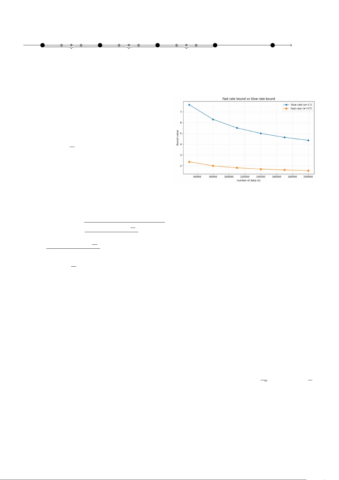
Uniform Error Bounds for Quan tized Dynamical Mo dels Ab delk ader Metak alard ∗ , ∗∗ F abien Lauer ∗∗ Kevin Colin ∗ Marion Gilson ∗ ∗ Universit ´ e de L orr aine, CNRS, CRAN, F-54000 Nancy, F r anc e (e-mail: firstname.lastname@u niv-lorr aine.fr) ∗∗ Universit ´ e de L orr aine, CNRS, LORIA, F-54000 Nancy, F r anc e (e-mail: firstname.lastname@ loria.fr) Abstract: This pap er pro vides statistical guarantees on the accuracy of dynamical models learned from dep enden t data sequences. Sp ecifically , we dev elop uniform error b ounds that apply to quantized mo dels and imp erfect optimization algorithms commonly used in practical con texts for system identification, and in particular h ybrid system identification. Two families of b ounds are obtained: slo w-rate b ounds via a block decomposition and fast-rate, v ariance- adaptiv e, bounds via a nov el spaced-p oin t strategy . The bounds scale with the n umber of bits required to encode the mo del and thus translate hardw are constrain ts in to in terpretable statistical complexities. Keywor ds: System identification, Statistical learning theory , dependent data 1. INTRODUCTION This paper lies at the intersection of system identification (Ljung, 1999), whic h aims at learning models of dynam- ical systems, and learning theory (V apnik, 1998), which pro vides statistical guarantees on the accuracy of mo dels learned from data. More sp ecifically , we concentrate on the question of obtaining high probability b ounds on the accuracy of mo dels learned from sequences of p ossibly dep enden t data, while taking practical considerations in to accoun t. In particular, the prop osed analysis holds for imp erfect algorithms (for instance those that cannot guar- an tee to minimize the empirical risk) and models imple- men ted on computing devices with finite precision. Indeed, lo cal optimization or heuristic metho ds are often used for learning in practice, when training neural netw orks (Go odfellow et al., 2016) or estimating hybrid dynamical systems (Lauer and Blo c h, 2019) for instance, and mo dels are more and more implemented with low precision due to limited hardw are capabilities (as with micro controllers) or latency and p o wer consumption restrictions (Jacob et al., 2018). 1.1 R elate d Work The main difficulty for pro viding nonasymptotic risk guar- an tees for system iden tification stems from the dependence b et w een data p oints that are collected at subsequent time steps along a single tra jectory of the modeled system. This issue has b een addressed from tw o complemen tary p erspectives in the literature. • Mixing–based learning theory: A first fam- ily of approaches extends classical tools from learn- ing theory to dep enden t data via mixing argumen ts (Y u, 1994; Meir, 2000; W eyer, 2000; Vidyasagar and Karandik a, 2004; Mohri and Rostamizadeh, 2009; Massucci et al., 2022). These analyses quantify the temp oral dep endence through co efficien ts (e.g., β – or θ –mixing ones) that capture the decay of correlations across time. Then, a decomp osition technique due to the seminal work of Y u (1994) yields bounds that apply to a subsample of the data. How ev er, the loss in terms of effective sample size is comp ensated by the v ersatility of the approach that can yield widely appli- cable and uniform error b ounds, i.e., results that are algorithm-indep enden t. Y et, these approac hes typi- cally rely on rather in v olved measures of the complex- it y of the mo del that must b e accurately analyzed b efore applying the b ounds, such as Rademacher complexities for Mohri and Rostamizadeh (2009), gro wth functions for McDonald et al. (2011), w eak- dep endence metrics for Alquier and Win tenberger (2012), or an information-theoretic div ergence for Eringis et al. (2024). • Algorithm–sp ecific finite–sample analyses without mixing: A second line of work provides sharp, problem tailored, guaran tees for sp ecific estimators and mo del classes, that are typically linear or w ell-structured, using self-normalized martingale to ols and related techniques (Simcho witz et al., 2018; F aradonbeh et al., 2018; Jedra and Prouti ` ere, 2023), as survey ed in (Tsiamis et al., 2023). When a closed-form expression of the estimator is av ailable, these results yield precise finite-sample rates. Their sp ecialization to a given algorithm-mo del pair makes them complementary to the uniform, algorithm–agnostic p erspective adopted b elo w. Notably , other w orks also consider a mid-p oin t b et w een these tw o types of approaches: Ziemann and T u (2022) deriv es strong guarantees for the sp ecific case of the least- squares estimator under mixing conditions. An imp ortan t area of application for the prop osed ap- proac h is hybrid system identification, as defined in Lauer and Bloch (2019), where the data-generating system switc hes b et ween different subsystems in an unobserved and unkno wn manner. Beside the issue of dep endence, this raises additional algorithmic difficulties that preven t the application of the algorithmic-sp ecific approaches men- tioned ab o v e. Statistical guarantees for hybrid systems w ere deriv ed in Chen and Poor (2022), but in a sligh tly differen t and simplified setting where the data is collected as multiple short and indep enden t tra jectories, each gen- erated by a single subsystem, thus alleviating some algo- rithmic issues and reducing the dependency issue. Other w orks, like Sattar et al. (2021), prop ose error b ounds for Mark ov jump systems, but under the simplifying as- sumption that the switc hings are observed or kno wn, in whic h case the problem b ecomes more closely related to the iden tification of m ultiple indep enden t linear systems and algorithmic-specific approaches can be more easily dev elop ed. 1.2 Contributions This pap er fo cuses on the deriv ation of widely applicable guaran tees that take in to account practical limitations often encoun tered in practice, b y follo wing the line of w ork based on mixing argumen ts. The proposed results tak e the form of probabilistic error b ounds that enjoy the follo wing prop erties. • Uniform o v er the mo del class. The b ounds hold for any mo del within the predefined class, and th us re- main indep enden t of the identification procedure and insensitiv e to algorithmic or optimization issues. This is particularly crucial for nonlinearly parametrized mo dels, suc h as neural net works, or hybrid system iden tification where complex learning problems are solv ed using heuristics. • Quan tization–aw are. The b ounds explicitly take the quan tization of mo dels in to accoun t via a com- plexit y term based on the num b er of bits used to enco de the mo del class. • Generalit y and In terpretability . The results co ver a broad range of linear, nonlinear and hybrid dynamical mo dels and are directly applicable to new mo del classes by merely measuring their bit-size. • F ast rates. W e provide a nov e l decomp osition tech- nique that we leverage to obtain fast-rate bounds that are b oth more efficient and easier to deriv e than with standard to ols. The resulting b ounds are also tighter than most results of the literature in many cases. • Simple deriv ations and explicit constan ts. The prop osed deriv ations remain simple enough to yield small and explicit constants, whic h are otherwise often to o conserv ative or merely ignored in other w orks. 1.3 Pap er Or ganization W e first introduces in Sect. 2 the learning framew ork b efore establishing a first bound for indep enden t data in Sect. 3. Next, we turn to dep enden t data, with b oth slow (Sect. 4) and fast (Sect. 5) rate b ounds. Finally , Section 6 presen ts numerical exp erimen ts that highlight the b enefit of the prop osed results, b efore concluding in Sect. 7. 2. LEARNING FRAMEWORK W e consider stationary sto c hastic pro cesses and establish the general framew ork b efore introducing quantization considerations. Let ( X t , Y t ) t ∈ Z b e a stationary sto chastic pro cess taking v alues in X × Y , with Y ⊂ [ − r , r ]. W e consider mo del classes F consisting of functions f : X → Y . F or a given loss function ℓ : Y × Y → [0 , M ], we define the risk (generalization error) of a mo del f ∈ F as: L ( f ) = E [ ℓ ( Y t , f ( X t ))] , where E denotes the exp ectation with resp ect to ( X t , Y t ), whic h, by stationarity , do es not dep end on t . Hyp othesis 1. The outputs Y t are b ounded within [ − r, r ], and the mo del f is clipp ed to ensure f ( X ) ∈ [ − r , r ]. Hyp othesis 1 ensures that the loss function remains b ounded. F or instance, the squared loss ℓ ( Y t , f ( X t )) = ( Y t − f ( X i )) 2 is often considered and bounded b y M = 4 r 2 under Hyp othesis 1. While clipping is a natural op eration when the outputs are kno wn to b e b ounded, Hyp othesis 1 basically requires the system to be stable, which consti- tutes the main limitation of the prop osed approac h. How- ev er, it could b e adapted to a more general setting using concen tration results for subgaussian or subexp onen tial distributions (V ersh ynin, 2025). Another basic assumption, often satisfied in practice, will b e crucial to our framework throughout the pap er: Hyp othesis 2. The learning algorithm outputs a function f within a parametric mo del class F that is implemented on a computer with a B -bits representation of real num b ers: F = { f ( · ; w ) : w ∈ W B } , (1) where f ( · ; w ) is parametrized by w , W ⊂ R p is the admissible set of parameters, W B is its quantized version o ver B -bits and p is the num b er of parameters. Note that w e do not require a precise definition of the en- co ding mechanism for real num bers: the results deriv ed b e- lo w hold similarly for all enco dings based on the same n um- b er of bits B (including both floating-p oin t and fixed-p oin t n umbers). Given a training sample ( X 1 , Y 1 ) , . . . , ( X n , Y n ), the empirical risk is: ˆ L n ( f ) = 1 n n X i =1 ℓ ( Y t , f ( X t )) . When the data are dep enden t, we rely on a mixing co ef- ficien t to measure this dep endence. A stationary pro cess ( Z t ) is β -mixing if its mixing co efficien ts β ( k ) conv erge to zero as k → ∞ , where, for any t : β ( k ) = sup A ∈ σ ( Z t −∞ ) ,B ∈ σ ( Z ∞ t + k ) | P ( A ∩ B ) − P ( A ) P ( B ) | , and σ ( Z t s ) denotes the σ -algebra generated by ( Z s , . . . , Z t ). Man y dynamical systems generate β -mixing pro cesses with exp onen tially decaying coefficients. Classical exam- ples studied in Doukhan (1994) include: • Linear systems: F or Y t +1 = AY t + η t with sp ectral radius ρ ( A ) < 1 and i.i.d. noise η t , the mixing rate is go verned b y the sp ectral radius: β ( k ) ≤ C ρ ( A ) k for some constan t C . In the univ ariate case ( Y t ∈ R ), this reduces to the autoregressive mo del Y t = θ Y t − 1 + η t with | θ | < 1, yielding β ( k ) ≤ C | θ | k . • Nonlinear autoregressiv e mo dels: Systems Y t = g ( Y t − 1 , . . . , Y t − p ) + η t where g satisfies Lipschitz con- ditions with sufficiently small constant exhibit β - mixing with exp onen tially decaying co efficien ts. 3. ERROR BOUNDS FOR QUANTIZED MODELS W e first introduce error b ounds for quan tized mo dels in the static case b efore extending to dynamical systems, in order to exhibit ho w quan tization affects statistical guarantees and demonstrate the b enefits of our approach in a simpler setting. Our first generalization error b ound b elo w relies on a quan tization of the parameter space as in Hyp othesis 2 that limits the cardinality of F to at most 2 B p , where p is the num b er of parameters and B the num b er of bits for eac h parameter. The or em 3. (Error b ound for indep enden t data). Assume ( X t , Y t ) are indep enden t and iden tically distributed (i.i.d.), and F is a mo del class as in Hyp othesis 2. Then, for an y δ ∈ (0 , 1), with probability at least 1 − δ , ∀ f ∈ F , L ( f ) ≤ ˆ L n ( f ) + M r B p ln 2 + ln(1 /δ ) n . Pro of. Let N = Card F ≤ 2 B p . Since ℓ is b ounded in [0 , M ], for each f ∈ F , Ho effding’s inequality gives: P  L ( f ) − ˆ L n ( f ) ≥ ϵ  ≤ exp( − 2 nϵ 2 / M 2 ) . Applying the union b ound ov er all f ∈ F , we get: P  ∃ f ∈ F , L ( f ) − ˆ L n ( f ) ≥ ϵ  ≤ N exp( − 2 nϵ 2 / M 2 ) . Setting the right-hand side equal to δ then yields ϵ 2 = M 2 log( N ) + log(1 /δ ) 2 n , and, since N ≤ 2 B p , ϵ ≤ M r B p log 2 + log (1 /δ ) n . Th us, with probability at least 1 − δ , for all f ∈ F , L ( f ) ≤ ˆ L n ( f ) + M r B p log 2 + log (1 /δ ) n . R emark 1. The term B p in the b ound of Theorem 3 cor- resp onds to the total num b er of bits necessary to sp ecify a quantized mo del, offering a practical and interpretable complexit y measure. This b ound pro vides for instance a direct guideline for selecting B in relation to n and p to balance estimation and quan tization (appro ximation) error. 4. ERROR BOUNDS FOR QUANTIZED DYNAMICAL MODELS W e now extend our analysis to dynamical systems by lev eraging the blo ck decomposition technique of Y u (1994). B 1 B 2 B 3 B 4 B 5 B 6 B 7 B 8 · · · Fig. 1. Tw o in tertwined blo c k sequences: ligh t gra y for S 1 , blac k for S 2 . The k ey idea is to decompose the sequence of length n in to blo c ks of size a to limit the dep endence b et ween observ ations taken from the o dd blo c ks only . Sp ecifically , given a sequence (( X t , Y t )) 1 ≤ t ≤ n and tw o in tegers a > 0 and µ > 0 such that 2 aµ = n , define the 2 µ blo c ks of length a , for j = 1 , . . . , µ , as B j =  ( X a ( j − 1)+1 , Y a ( j − 1)+1 ) , . . . , ( X aj , Y aj )  . This yields tw o intert wined sequences of blo c ks, S 1 = B 1:2:2 µ − 1 = ( B 1 , B 3 , B 5 , . . . , B 2 µ − 1 ) (2) S 2 = B 2:2:2 µ = ( B 2 , B 4 , B 6 , . . . , B 2 µ ) as illustrated in Fig. 1, whic h provide the basis for the pro of of the following result, as detailed in App endix B. The or em 4. Let F b e a quantized mo del class as in Hy- p othesis 2 and, for any δ ∈ (0 , 1), let δ ′ = δ − 2( µ − 1) β ( a ) > 0. Then, with probability at least 1 − δ , ∀ f ∈ F , L n ( f ) ≤ ˆ L n ( f ) + M s 2(( B p + 1) ln 2 + ln 1 δ ′ ) µ . Here again, the complexity of the mo del is measured in a straightforw ard manner by the num ber of bits B and the n umber of parameters p . The dynamical nature of this b ound, in comparison with Theorem 3, app ears in δ ′ , which includes the mixing co efficien t β ( a ), and implies a slightly larger v alue of the corresp onding log term. Another consequence is the fact that the confidence index δ cannot b e set smaller than 2( µ − 1) β ( a ). Conv ersely , the blo c k size a m ust be prop erly c hosen with the follo wing trade-off in mind. On the one hand, a large v alue of a reduces the mixing penalty β ( a ), but decreases the effectiv e sample size µ = n/ (2 a ), which increases the confidence interv al ∝ p 1 /µ . On the other hand, a small v alue of a increases µ and improv es the b ound, but also increases β ( a ), which might lead to a violation of δ ′ > 0. In practice, it is often b est to c ho ose the smallest v alue of a in order to satisfy δ ′ > 0, as will be illustrated b y T able 1 in Sect. 6.1. 5. F AST RA TE BOUNDS While blo ck decomp osition is an effective to ol for ob- taining generalization b ounds with dep endent ( β -mixing) data, it encounters inherent limitations for achieving fast- rate (v ariance-dependent) b ounds. This is mainly b ecause dep endence within eac h blo c k means that the empirical v ariance computed on the blo cks do es not accurately re- flect the actual v ariance of the pro cess, thus preven ting meaningful Bernstein-type inequalities. As a result, the obtained rates are p essimistic or the constants ov erly large, and such b ounds rarely improv e ov er the standard “slow rate”. T o address this issue, we introduce b elo w a new approach based on selecting p oints that are sufficiently spaced in time, whic h allows for sharp er and more interpretable fast- rate generalization b ounds. Indeed, indep enden t copies Index t 1 a + 1 2 a + 1 3 a + 1 a p oin ts a p oin ts a p oin ts · · · ( µ ′ − 1) a + 1 Fig. 2. Spaced p oin t selection in (3), showing the first four and the last p oin ts, with a p oints b et ween each pair. of the spaced p oints can b e considered, for which the v ariance entering a Bernstein-type inequality can b e easily con trolled via the true risk. F ormally , the spaced-p oints tec hnique, illustrated by Fig. 2, considers a subsample of µ ′ spaced p oin ts S a =  ( X 1+( k − 1) a , Y 1+( k − 1) a )  1 ≤ k ≤ µ ′ , (3) where a is the spacing parameter and µ ′ = ⌊ n/a ⌋ is the effectiv e sample size used to computed the empirical risk ˆ L spaced n ( f ) = 1 µ ′ µ ′ X k =1 ℓ ( Y 1+( k − 1) a , f ( X 1+( k − 1) a )) . R emark 2. Notice that since µ ′ is equal to 2 µ , the effectiv e sample size for this approac h will b e twice the one obtained b y the classical decomp osition into blo c ks. In this setting, the following error b ound can b e prov ed, as detailed in App endix C. The or em 5. (F ast-rate b ound). Let F b e a quantized mo del class as in Hypothesis 2, and, for an y δ ∈ (0 , 1), let δ ′′ = δ − ( µ ′ − 1) β ( a ) > 0. Then, with probability at least 1 − δ , uniformly ov er all f ∈ F , L n ( f ) ≤ ˆ L spaced n ( f ) + s 2 M B p ln(2) + ln( 1 δ ′′ ) µ ′ ˆ L spaced n ( f ) + 4 M B p ln(2) + ln( 1 δ ′′ ) µ ′ (4) The b ound of Theorem 5 combines tw o confidence inter- v als, one in O (1 / √ µ ′ ) and one in O (1 /µ ′ ). How ever, the first one includes the empirical risk ˆ L spaced n ( f ) and v anishes as the model f fits more accurately the data, leading to an effectiv e fast conv ergence rate of O (1 /µ ′ ) in low empirical error cases. R emark 3. (Blo ck decomp osition approach and fast rates). A result in the spirit of Theorem 5 could be obtained with the standard block decomp osition technique of Y u (1994) that we used in Sect. 4. How ev er, the fast rate of Theorem 5 is obtained b y taking into accoun t the v ariance of the pro cess in the deriv ations. Such an approach based on blocks w ould hav e to deal with the v ariance of blo cks, which is itself impacted by the co v ariance b et w een dep enden t data p oin ts tak en from the same blo c k. This would lead to additional terms, an extra level of complexity and an ov erall less efficient approach than the one we prop ose ab o ve. 6. EXAMPLES This section presents tw o example applications of the prop osed b ounds. Section 6.1 considers a simple linear sys- tem for which the β -mixing co efficien ts can b e accurately estimated. This lets us compute the full b ound including mixing terms and exhibit the practical gain of the fast- rate b ound. Then, Section 6.2 shows ho w the prop osed approac h easily handles h ybrid system identification, to whic h very few others apply beside the one of Massucci et al. (2022). Fig. 3. Slow and fast rate error b ounds as functions of n when mo deling (5). 6.1 Line ar system identific ation W e first consider a stationary AR(1) time series Y t = θ Y t − 1 + η t , η t i.i.d. ∼ N (0 , 1) , θ = 0 . 5 , (5) with n = 200 , 000 observ ations. W e learn ˆ θ by ordinary least squares with X t = Y t − 1 . T o keep the squared loss b ounded b y M = 4 r 2 , we clip b oth data and mo del outputs at r = 3. W e assume a quan tized mo del class with p = 1 parameter stored on B = 32 bits. T o compute the b eta- mixing co effcient, we use the metho d of McDonald et al. (2011). T able 1 rep orts the empirical risks (from the same sim- ulation), the confidence in terv als, and the o v erall b ound for Theorems 4 and 5 for several v alues of a . Here, the v alue of a starts at 17, in order to satisfy the constraints δ ′ > 0 and δ ′′ > 0. These results show that computing the empirical risk on fewer data p oin ts, as with ˆ L spaced n ( f ), do es not significantly impact its v alue: ˆ L spaced n ( f ) is very close to ˆ L n ( f ) is all tests. Therefore, the fast-rate b ound of Theorem 5 is alwa ys b etter than the other one. T able 1 also sho ws that, as a increases, both µ and µ ′ decrease, whic h results in an increase of the confidence interv als and the ov erall b ounds. Figure 3 shows how the tw o b ounds decrease monotonically with n , as b oth µ and µ ′ gro w linearly with n , with rates O ( 1 √ µ ) and almost O ( 1 µ ′ ), resp ectiv ely . and 6.2 Switche d system identific ation Hybrid systems are systems that switch b et ween differen t op erating modes. Here, we focus on arbitrarily switched linear systems of the form y t = f s t ( x t ) + η t , f j ( x t ) = w T j x t , j = 1 , . . . , C, (6) T able 1. Comparison b et ween the slow and fast rate b ounds on the linear system identification example of Sect. 6.1 for δ = 0 . 05 and v arious blo c k sizes a . Slo w (Theorem 4) F ast (Theorem 5) a µ ˆ L n ( f ) Confidence interv al T otal µ ′ ˆ L spaced n ( f ) Confidence interv al T otal 17 5882 0.9823 3.312 4.355 11764 0.9869 0.630 1.691 21 4761 0.9823 3.701 4.683 9523 0.9650 0.729 1.766 25 3999 0.9823 4.036 5.018 7999 0.9862 0.834 1.902 30 3333 0.9823 4.421 5.403 6666 0.9820 0.954 2.031 40 2499 0.9823 5.105 6.088 4999 0.9679 1.183 2.270 where y t ∈ R is the output, x t ∈ X ⊂ R d the regression v ector, s t ∈ { 1 , . . . , C } the discrete state or mo de, C the n umber of submo dels, f j with j ∈ { 1 , . . . , C } the linear submo del of parameters w j ∈ R d and η t ∈ R a noise term. The regressor x t ∈ R d , d = n a + n b , with the mo del orders n a and n b , is given b y x t = [ y t − 1 , . . . , y t − n a , u t − 1 , . . . , u t − n b ] T , (7) where the u t − k ’s denote the delay ed inputs. In hybrid sys- tem identification (Lauer and Blo c h, 2019), the switching sequence ( s t ) is assumed unknown and the problem is to estimate the submo dels f j from the ( x t , y t )’s only , whic h is t ypically done by minimizing the p oint wise switching loss ℓ ( f , x, y ) = min j ∈{ 1 ,...,C } ( y − f j ( x )) 2 . (8) Since this loss function is nonconv ex (and not differen- tiable), its minimization is a difficult task often handled b y heuristic algorithms for which the estimated mo del cannot b e characterized a priori (except in some specific cases). Thus, statistical guaran tees in the fla v or of those review ed by Tsiamis et al. (2023) do not apply and uniform b ounds m ust b e considered. The only other approach that pro vides error b ounds in this sp ecific context is the one of Massucci et al. (2022) based on Rademacher complexities. F or switched linear systems of the form (6), it yields L ( f ) ≤ ˆ L n ( f ) + 16 r Λ q C P µ i =1 ∥ X 2 a ( i − 1)+1 ∥ 2 2 µ | {z } Rademacher complexity (mixing–free) (9) + 12 r 2 s log(4 /δ ′′′ ) 2 µ | {z } mixing part , where δ ′′′ = δ − 4( µ − 1) β ( a ) and Λ is an upp er b ound on the mo del complexity as measured by q P C j =1 ∥ w j ∥ 2 2 . Here, w e compare b ound (9) with Theorems 4–5. Since estimating the β -mixing coefficients remains a complex task out of the scope of this pap er, t wo levels of comparison are considered. One lev el concentrates on the parts of the b ounds that do not dep end on the mixing co efficients (as detailed in App endix D), and another one computes the v alues of the b ounds for a v alue of the confidence indexes arbitrarily set to δ ′ = δ ′′ = δ ′′′ = 0 . 01. The comparison is based on an example switched system tak en from Massucci et al. (2022) with n a = n b = 2 and C = 3 mo des of parameters T able 2. Comparison of error b ounds for switc hed system identification. Bound F ull confidence Complexity term interv al (mixing-free) (with mixing) Massucci et al. (2022), (9) 23.48 27.77 Theorem 4, (D.1) 19.06 19.23 Theorem 5, (D.2) 10.23 10.41 w 1 =    − 0 . 4 0 . 25 − 0 . 15 0 . 08    , w 2 =    1 . 55 − 0 . 58 − 2 . 10 0 . 96    , w 3 =    1 . 00 − 0 . 24 − 0 . 65 0 . 30    , (10) input u t ∼ N (0 , 1), and white output noise η t with a signal-to-noise ratio of = 30 dB, ov er n = 80 000 data p oin ts. The mode s t is uniformly dra wn at random at eac h time step. Clipping is applied to b oth data and mo del outputs with r = 3. Theorems 4–5 are applied with a total n umber of parameters p = C d = 12, with B = 32 bits p er parameter. The bound of Massucci et al. (2022) is applied with Λ = q P C j =1 ∥ w j ∥ 2 2 computed with (10) and th us as a tight upp er b ound on the true mo del complexity (whic h is the most fa vorable case for this b ound). F or both approac hes, the blo c k length is set to a = 21, which leads to µ = ⌊ n/ (2 a ) ⌋ = 1904 and µ ′ = ⌊ n/a ⌋ = 3809. R esults. T able 2 rep orts the mixing-free parts of the confidence in terv al and the total confidence in terv al v alues in the settings discussed abov e and for the three compared b ounds. These results again sho w the notable adv antage of the fast rate of Theorem 5, which also b enefits from the twice larger effectiv e sample size µ ′ = 2 µ that could not b e obtained with the standard blo ck decomp osition approac h. Regarding b ound (9), the difference betw een the t wo rep orted v alues reflects the larger constant in front of the mixing part. 7. CONCLUSIONS This pap er developed uniform error b ounds for quantized dynamical mo dels that address key limitations of existing theoretical guarantees. Our results apply to general mo del classes, accoun t for quantization effects, and provide ex- plicit constan ts with improv ed magnitude. The bounds are uniform with resp ect to the iden tification algorithm and th us relev ant for practical implemen tations using heuristic optimization metho ds, as is often the case in e.g. h ybrid system identification. In addition, a v ersion with a fast con vergence rate w as deriv ed with a nov el decomp osition approac h and prov ed b eneficial in numerical exp erimen ts. F uture w ork ma y explore extensions to non-stationary pro cesses and adaptiv e spacing strategies for the no v el decomp osition technique. REFERENCES Alquier, P . and Winten berger, O. (2012). Mo del selection for weakly dep enden t time series forecasting. Bernoul li , 18(3), 883–913. Chen, Y. and Poor, H.V. (2022). Learning mixtures of linear dynamical systems. In International c onfer enc e on machine le arning (ICML) . PMLR. Doukhan, P . (1994). Mixing: Pr op erties and Examples . Springer-V erlag. Eringis, D., Leth, J., T an, Z.H., Wisniewski, R., and Pe- treczky , M. (2024). P AC-ba yes generalisation b ounds for dynamical systems including stable RNNs. In Pr o c e e d- ings of the AAAI Confer enc e on Artificial Intel ligenc e , v olume 38, 11901–11909. F aradon b eh, M.B., T ewari, A., and Michailidis, G. (2018). Finite time identification in unstable linear systems. A utomatic a , 96, 342–353. Go odfellow, I., Bengio, Y., and Courville, A. (2016). De ep L e arning . MIT Press. Jacob, B., Kligys, S., Chen, B., Zhu, M., T ang, M., Ho ward, A., Adam, H., and Kalenichenk o, D. (2018). Quan tization and training of neural netw orks for effi- cien t integer-arithmetic-only inference. In Pr o c e e dings of the IEEE Confer enc e on Computer Vision and Pattern R e c o gnition (CVPR) , 2704–2713. Jedra, Y. and Prouti` ere, A. (2023). Finite-time identifica- tion of linear systems: F undamental limits and optimal algorithms. IEEE T r ansactions on Automatic Contr ol , 68, 2805–2820. Lauer, F. and Blo ch, G. (2019). Hybrid system identifi- c ation: The ory and Algorithms for L e arning Switching Mo dels . Springer. Ljung, L. (1999). System Identific ation: The ory for the User . Prentice Hall PTR. Massucci, L., Lauer, F., and Gilson, M. (2022). A sta- tistical learning persp ective on switc hed linear system iden tification. A utomatic a , 145, 110532. McDonald, D., Shalizi, C., and Schervish, M. (2011). Es- timating b eta-mixing co efficien ts. In Pr o c e e dings of the 14th International Confer enc e on Artificial Intel ligenc e and Statistics , v olume 15 of Pr o c e e dings of Machine L e arning R ese ar ch , 516–524. Meir, R. (2000). Nonparametric time series prediction through adaptive model selection. Machine L e arning , 39, 5–34. Mohri, M. and Rostamizadeh, A. (2009). Rademacher complexit y b ounds for non-iid pro cesses. In A dvanc es in Neur al Information Pr o c essing Systems (NeurIPS) , 1097–1104. Sattar, Y. et al. (2021). Identification and adaptive control of mark ov jump systems: Sample complexity and regret b ounds. arXiv pr eprint arXiv:2111.07018 . Simc howitz, M., Mania, H., T u, S., Jordan, M.I., and Rec ht, B. (2018). Learning without mixing: T ow ards a sharp analysis of linear system identification. In Pr o c e e dings of the 31st Confer enc e on L e arning The ory (COL T) , 439–473. Tsiamis, A., Ziemann, I., Matni, N., and P appas, G.J. (2023). Statistical learning theory for control: A finite- sample persp ectiv e. IEEE Contr ol Systems Magazine , 43, 67–97. V apnik, V.N. (1998). Statistic al L e arning The ory . Wiley . V ersh ynin, R. (2025). High-Dimensional Pr ob ability . Cam- bridge Univ ersity Press, 2nd edition edition. Vidy asagar, M. and Karandik a, R. (2004). A learning theory approac h to system iden tification. In Pr o c. of the 7th IF AC Symp osium on A dvanc e d Contr ol of Chemic al Pr o c esses (ADCHEM), Hong Kong, China , 1–9. W ey er, E. (2000). Finite sample prop erties of system iden tification of arx models under mixing conditions. A utomatic a , 36(9), 1291–1299. Y u, B. (1994). Rates of conv ergence for empirical pro- cesses of stationary mixing sequences. The Annals of Pr ob ability , 22(1), 94–116. Ziemann, I. and T u, S. (2022). Learning with little mixing. A dvanc es in Neur al Information Pr o c essing Systems , 35, 4626–4637. App endix A. TECHNICAL LEMMAS W e recall the follo wing seminal result on β -mixing se- quences. L emma 6. (Lemma 4.1 in Y u (1994)). Giv en a sequence of random v ariables ( Z i ) 1 ≤ i ≤ n ∈ Z n of mixing co efficien ts β ( k ), decomp osed into blo c ks as in (2), and a b ounded function g : Z aµ → [ − g , g ], | E g ( S 1 ) − E g ( S ′ ) | ≤ ( µ − 1) g β ( a ) , (A.1) where S ′ is an indep endent sequence of blo c ks with the same marginal distribution for each blo c k as for S 1 but with indep enden t blo c ks. W e also pro vide a slight mo dification of this result that will b e used at the core of the proposed space-points tec hnique, and that holds as a direct consequence of Corollary 2.7 in Y u (1994). L emma 7. (Coupling Lemma for Spaced P oints). Let ( Z i ) 1 ≤ i ≤ n b e a stationary sequence of real-v alued random v ariables with β –mixing co efficien ts β ( k ). Fix an in teger spacing a ≥ 1 so that µ ′ = ⌊ n/a ⌋ and let g : R µ ′ → [ − g , g ] b e any b ounded function. Define the sp ac e d sample S =  Z 1 , Z 1+ a , . . . , Z 1+( µ ′ − 1) a  , and let S ′ = ( Z ′ 1 , . . . , Z ′ µ ′ ) b e a sequence of indep enden t v ariables with the same marginal distribution for each Z ′ k as Z 1+( k − 1) a . Then | E g ( S ) − E g ( S ′ ) | ≤ ( µ ′ − 1) g β ( a ) . App endix B. PROOF OF THEOREM 4 Consider the blo c k decomp osition of (2) and, for every f ∈ F , define the blo c k av erages h f ( B j ) := 1 a a X i =1 ℓ  Y a ( j − 1)+ i , f ( X a ( j − 1)+ i )  . and note that each h f ( B j ) is bounded in [0 , M ] as the loss function. F or k ∈ { 1 , 2 } define the deviations ∆ S k ( f ) := E h f ( B 1 ) − 1 µ µ − 1 X j =0 h f ( B k +2 j ) = L n ( f ) − 1 µ µ − 1 X j =0 h f ( B k +2 j ) . (B.1) W e enco de the corresp onding large deviation even t with the indicator function 1 {∃ f ∈F : ∆ S k ( f ) ≥ ε } , whic h is b ounded b y 1. Then, each probabilit y can b e computed as P {∃ f : ∆ S k ( f ) ≥ ε } = E 1 {∃ f ∈F : ∆ S k ( f ) ≥ ε } (B.2) and, by Lemma 6, for each k ∈ { 1 , 2 } there exists an i.i.d. sequence of blo cks S ′ k (comp osed of i.i.d. blo c ks with the same marginals as the blo c ks of S k ) suc h that E 1 {∃ f ∈F : ∆ S k ( f ) ≥ ε } ≤ E 1 {∃ f ∈F : ∆ S ′ k ( f ) ≥ ε } + ( µ − 1) β ( a ) . (B.3) On the other hand, since the blo c ks of S ′ k are independent, Ho effding’s inequality yields, for any f and any ε > 0, P n ∆ S ′ k ( f ) ≥ ε o ≤ exp  − µ ε 2 M 2  . T aking a union b ound ov er f ∈ F (with |F | = 2 B p ) giv es P n ∃ f ∈ F : ∆ S ′ k ( f ) ≥ ε o ≤ 2 B p exp  − µε 2 M 2  . Com bining with (B.2) and (B.3), for each k ∈ { 1 , 2 } , P {∃ f ∈ F : ∆ S k ( f ) ≥ ε } ≤ 2 B p exp  − µε 2 M 2  +( µ − 1) β ( a ) . (B.4) By a further union b ound applied to (B.4) for k = 1 and k = 2, P {∃ f ∈ F : max { ∆ S 1 ( f ) , ∆ S 2 ( f ) } ≥ ε } ≤ 2 B p +1 exp  − µε 2 M 2  + 2( µ − 1) β ( a ) . (B.5) Let δ ′ = δ − 2( µ − 1) β ( a ) > 0 and choose ε > 0 so that 2 B p +1 exp  − µ ε 2 M 2  = δ ′ This yields ε = M s 2  ( B p + 1) ln 2 + ln(1 /δ ′ )  µ . Then, (B.5) implies that, with probabilit y at least 1 − δ , sim ultaneously for all f ∈ F , ∆ S 1 ( f ) ≤ ε and ∆ S 2 ( f ) ≤ ε. Using (B.1), the tw o inequalities ab o ve are equiv alen t to L n ( f ) ≤ 1 µ µ − 1 X j =0 h f ( B 1+2 j ) + ε and L n ( f ) ≤ 1 µ µ − 1 X j =0 h f ( B 2+2 j ) + ε whic h ensures that L n ( f ) ≤ 1 2   1 µ µ − 1 X j =0 h f ( B 1+2 j ) + 1 µ µ − 1 X j =0 h f ( B 2+2 j )   + ε = ˆ L n ( f ) + ε. App endix C. PROOF OF THEOREM 5 W e start from the set of p oin ts introduced in (3) and define the deviation ∆ S a ( f ) = L n ( f ) − 1 µ ′ X ( X t ,Y t ) ∈ S a ℓ ( Y t , f ( X t )) = L n ( f ) − ˆ L spaced n ( f ) . Then, we enco de the deviation even t by the indicator (b ounded by 1) as Ψ ε ( S a ) = 1 ∃ f ∈F : ∆ S a ( f ) ≥ ε suc h that E Ψ ε ( S a ) = P { ∃ f ∈ F : ∆ S a ( f ) ≥ ε } . (C.1) Successiv e elements in S a are separated by exactly a indices of the original pro cess. By Lemma 7, there exists an i.i.d. sequence S ′ a :=  ( X ′ 1 , Y ′ 1 ) , . . . , ( X ′ µ ′ , Y ′ µ ′ )  , with ( X ′ j , Y ′ j ) distributed as ( X 1+( j − 1) a , Y 1+( j − 1) a ) such that E Ψ ε ( S a ) ≤ E Ψ ε ( S ′ a ) + ( µ ′ − 1) β ( a ) . (C.2) Fix f ∈ F and recall that ℓ ( Y t , f ( X t )) is b ounded in [0 , M ] with mean L n ( f ). Then, Bernstein’s inequality implies, for an y ε > 0, P  ∆ S ′ a ( f ) ≥ ε  ≤ exp − µ ′ ε 2 2 σ 2 f + 2 3 M ε ! , where σ 2 f is the v ariance of ℓ ( Y t , f ( X t )). T aking a union b ound ov er f ∈ F (with Card F = 2 B p ) giv es P  ∃ f ∈ F : ∆ S ′ a ( f ) ≥ ε  ≤ 2 B p exp − µ ′ ε 2 2 σ 2 f + 2 3 M ε ! . (C.3) Com bining (C.1), (C.2) and (C.3) yields P n ∃ f ∈ F : L n ( f ) − ˆ L spaced n ( f ) ≥ ε o (C.4) ≤ 2 B p exp  − µ ′ ε 2 2 σ 2 f + 2 3 M ε  + ( µ ′ − 1) β ( a ) . Set δ ′′ = δ − ( µ ′ − 1) β ( a ) and A = ln(2 B p /δ ′′ ). Enforce 2 B p exp − µ ′ ε 2 2 σ 2 f + 2 3 M ε ! = δ ′ ⇔ µ ′ ε 2 2 σ 2 f + 2 3 M ε = A. Multiplying b oth sides b y 2 σ 2 f + 2 3 M ε leads to a quadratic equation in ε : µ ′ ε 2 − 2 A 3 M ε − 2 Aσ 2 f = 0 . Solving for ε using the quadratic formula yields ε = 2 A 3 M + r  2 A 3 M  2 + 4 µ ′ · 2 Aσ 2 f 2 µ ′ . Using √ S 2 + T ≤ S + √ T with S = 2 A 3 M , T = 4 µ ′ A σ 2 f , giv es ε ≤ 2 M A 3 µ ′ + s 2 σ 2 f A µ ′ . Since ℓ ( Y t , f ( X t )) ∈ [0 , M ], w e ha ve the standard env e- lop e–v ariance b ound σ 2 f = V ar ( ℓ ( Y t , f ( X t ))) ≤ E [ ℓ ( Y t , f ( X t )) 2 ] ≤ M E [ ℓ ( Y t , f ( X t ))] = M L n ( f ) , whic h yields, together with (C.4), that the following holds with probabilit y at least 1 − δ : L n ( f ) ≤ ˆ L spaced n ( f ) + s 2 M A µ ′ L n ( f ) + 2 M A 3 µ ′ . (C.5) Set b = s 2 M A µ ′ , c = ˆ L n ( f ) + 2 M A 3 µ ′ . Then the inequalit y (C.5) b ecomes L n ( f ) ≤ b p L n ( f ) + c and b y the fact that 1 L n ( f ) ≤ b p L n ( f ) + c = ⇒ L n ( f ) ≤ b 2 + b √ c + c, w e obtain L n ( f ) ≤ 2 M A µ ′ | {z } b 2 + s 2 M A µ ′ s ˆ L n ( f ) + 2 M A 3 µ ′ | {z } b √ c + ˆ L n ( f ) + 2 M A 3 µ ′ | {z } c . Using √ x + y ≤ √ x + √ y , we write s ˆ L spaced n ( f ) + 2 M A 3 µ ′ ≤ q ˆ L spaced n ( f ) + s 2 M A 3 µ ′ . Hence b √ c ≤ s 2 M A µ ′ q ˆ L spaced n ( f ) + s 2 M A µ ′ s 2 M A 3 µ ′ ≤ s 2 M A µ ′ ˆ L spaced n ( f ) + 2 M A √ 3 µ ′ . Th us, the terms in O (1 /µ ′ ) sum to 2 M A  1 µ ′ + 1 3 µ ′ + 1 √ 3 µ ′  ≈ 3 . 82 M A µ ′ < 4 M A µ . Putting ev erything together, we see that (C.5) implies L n ( f ) ≤ ˆ L spaced n ( f ) + s 2 M A µ ′ ˆ L spaced n ( f ) + 4 M A µ ′ , in whic h replacing A by its v alue completes the pro of. App endix D. EXTRACTING MIXING-FREE P AR TS FR OM THE BOUNDS The confidence interv al in the b ound of Theorem 4 can b e decomp osed into a sum of t w o terms using the ubadditivity of the square ro ot with: β –free part = M s 2 ( B p + 1) ln 2 µ (D.1) mixing add-on = M s 2 ln(1 /δ ′ ) µ . F or the b ound of Theorem 5, let A 0 = B p ln 2. Again by √ x + y ≤ √ x + √ y , 1 This can b e prov ed by studying the sign of the quadratic p oly- nomial q ( α ) = α 2 − bα − c for α = p L n ( f ), the argument relies on computing the discriminant of q identifying the interv al where q ( α ) ≤ 0 and then squaring the resulting b ound on α . β –free part = s 2 M ˆ L spaced n A 0 µ ′ | {z } v ariance core + 4 M A 0 µ ′ | {z } linear core (D.2) mixing add-ons = s 2 M ˆ L spaced n ln 1 δ ′ µ ′ | {z } v ariance mixing + 4 M ln 1 δ ′ µ ′ | {z } linear mixing .