A Universal Neural Receiver that Learns at the Speed of Wireless

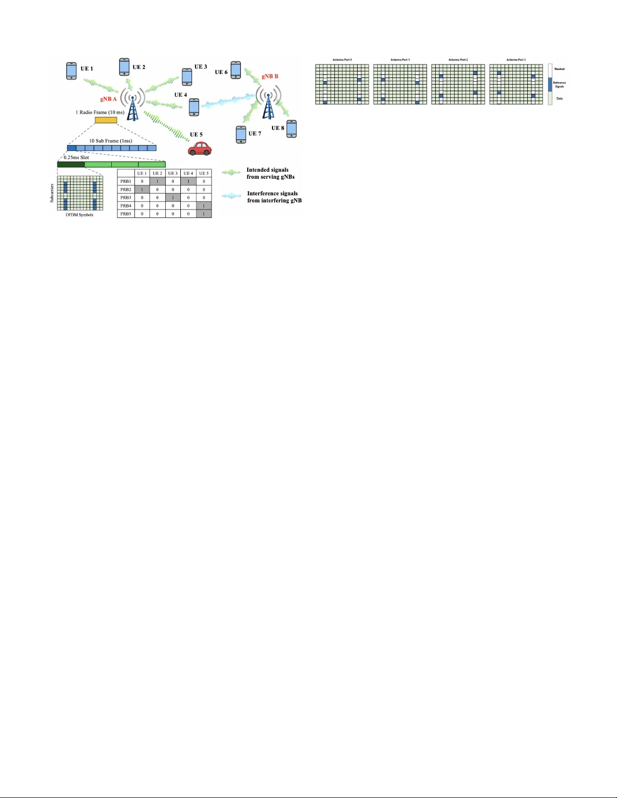
1 A Uni v ersal Neural Recei ver that Learns at the Speed of W ireless Lingjia Liu, Lizhong Zheng, Y ang Y i, and Robert Calderbank Abstract —T oday we design wireless networks using mathemat- ical models that gover n communication in different pr opagation en vironments. W e rely on measurement campaigns to deliver parametrized propagation models, and on the 3GPP standards process to optimize model-based performance, but as wireless networks become more complex this model-based approach is losing ground. Mobile Network Operators (MNOs) are counting on Artificial Intelligence (AI) to transform wireless by increasing spectral efficiency , reducing signaling overhead, and enabling continuous network innovation thr ough software upgrades. They may also be interested in new use cases like integrated sensing and communications (ISA C). All we need is an AI-native physical layer , so why not simply tailor the offline AI algorithms that hav e rev olutionized image and natural language processing to the wireless domain? W e argue that these algorithms rely on off-line training that is precluded by the sub-millisecond speeds at which the wireless interfer ence en vironment changes. W e present an alternativ e architectur e, a universal neural receiver based on conv olution, which gover ns transmit and recei ve signal processing of any signal in any part of the wireless spectrum. Our neural r eceiver is designed to in vert con volution, and we separate the question of which con volution to invert from the actual decon volution. The neural network that performs decon volution is very simple, and we configure this network by setting weights based on domain knowledge. By telling our neural network what we know , we av oid extensive offline training . By developing a universal receiver , we hope to simplify discussions about the proper choice of wav eform for different use cases in the international standards. Since the receiver architectur e is largely independent of technologies introduced at the base station, we hope to increase the rate of innovation in wireless. I . I N T R O D U C T I O N “ AI and communication” is one of the six key usage sce- narios of IMT -2030 [1]. Besides the communication aspect of requiring high area traf fic capacity and user-e xperienced data rates to support distributed computing and AI applications, this usage scenario is also expected to include a set of new capabilities related to the integration of AI and compute functionalities into IMT -2030 as illustrated in the concept of AI-enabled cellular networks [2]. As a critical step, the 3rd Generation Partnership Project (3GPP) has initiated the exploration of AI in the 6G air interface [3]. This trend of standardizing and deploying AI for the air interface is antici- pated to continue and ev olve through 6G/NextG networks. The growing interests in this domain mainly arise from the intrinsic issues of network complexity , model deficit , and algo- rithm deficit as detailed in [2], but tailored towards the air in- terface of the NextG mobile broadband networks. Specifically , L. Liu and Y . Yi are with Wireless@V irginia T ech, Bradley Department of ECE at V irginia T ech. L. Zheng is with the EECS Department at the Massachusetts Institute of T echnology (MIT), and R. Calderbank is with the ECE Department at Duke University . the air interface of the NextG (e.g., 6G and beyond) is ex- pected to be increasingly sophisticated with complex network topologies/numerologies, non-linear device components, and high-complexity processing algorithms. Therefore, it becomes exceedingly challenging to utilize conv entional model-based approaches in a scalable and efficient manner . Meanwhile, AI/ML-based data-driv en approaches can effecti vely resolve these issues, providing an appealing alternativ e for the design of the NextG air interface. Most of the introduced AI/ML-based strategies are focusing exclusi vely on tailoring the offline training that have rev olu- tionized image and natural language processing to the NextG air interface [3]. Howe ver , very little success has been reported so far . Why? One fundamental challenge is that 5G/NextG is a global technology , so models based on extensiv e offline training in New Y ork City may disappoint when deployed in Delhi, or ev en in Dallas. A second fundamental challenge is machine learning at the Speed of W ireless. Is it even possible to learn in a sub-millisecond transmit time interval (TTI) when the propagation en vironment is changing very rapidly in the NextG air interface? In this paper , we develop machine learning methods that are inspired by and based on the traditional model-based approaches to learn at the Speed of Wireless in the NextG air interface. W e start from con volution, which gov erns the transmission and reception of any wav eform in any part of the radio spectrum. By starting with a physical process that is common to all modes of wireless communication we are able to dev elop a univ ersal receiv er . Specifically , we present a neural receiv er that is designed to in vert conv olution. W e describe how it is able to implement online, real-time learning within each TTI without offline training for sev eral physical layer (PHY) wav eforms. The key to achieving computational efficienc y is to separate the question of which con volution to in vert from the actual decon volution. The neural network that performs decon volution is very simple, and we configure this network by setting the weights of the underlying neural network based on domain knowledge. By telling our neural network what we know , we av oid extensi ve offline training . The org anization of the paper is the following: Section II will introduce the dynamic nature of the radio environments of 5G and NextG in the air interface. The inherent challenges and potential solutions of applying AI/ML in the NextG air interface will be discussed in Section III. The uni versal neural receiver will be introduced in Section IV with its basic principles, the geometric interpretation for its explainability as well as case studies for weight configuration for both MIMO- OFDM and OTFS. Section V will contain the conclusion and 2 Fig. 1: Speed of W ireless in the Air Interface. the research outlook. I I . T H E S P E E D O F W I R E L E S S I N T H E A I R I N T E R FAC E The radio connections between mobile de vices (termed UEs by 3GPP) and base stations (termed gNBs by 3GPP) define the air interface of a mobile broadband cellular network. If AI/ML is to transform NextG networks, then we need to meet the challenge of integrating AI/ML into the air interface, where interference changes on a sub-millisecond time scale. Figure 1 sho ws a current 5G/5G-Advanced air interface where 2 gNBs serve 8 UEs, with gNB A serving 5 UEs and gNB B serving the remaining 3 UEs. Data is partitioned into 10 ms radio frames for transmission ov er the radio link between gNB A and UE 1 , and each radio frame is further divided into 10 subframes each of duration 1 ms. Then, depending on the numerology , each subframe will be further partitioned into 1 , 2 , 4 , 8 , or 16 slots with time duration ranging from 1 ms to 62 . 5 µ s. The transmission time interval (TTI), comprising one or more slots, is the granularity at which the 5G/5G- Advanced air interface assigns resources – subcarriers in the frequency domain and OFDM symbols in the time domain. The 6G/NextG air interface will be ev en more sophisticated. Scheduling Granularity and Complexity: Resources are partitioned into physical resource blocks (PRBs) consisting of 12 subcarriers (to provide frequency div ersity) which the gNB assigns to a single user (single-user scheduling) or to multiple users (multi-user scheduling) during each TTI. There may be 100 s of activ e UEs within a cell, and the typical number of PRBs in a 5G/5G-Adv anced air interface is between 50 and 70 . A UE is assigned a block of PRBs, and the gNB schedules PRBs to provide smooth Quality of Service. The number of scheduling options is astronomical. For simplicity , consider the do wnlink in Figure 1 where gNB A has 5 a v ailable PRBs to serve 5 active UEs. For single-user scheduling, where each PRB is scheduled to at most one UE, there are 6 5 possible scheduling options. For multiple-input multiple- output (MIMO) scheduling, gNB A can schedule multiple users on a PRB. If we limit gNB A to scheduling at most 2 UEs in each PRB, there are (6 × 5) 5 possible options. Figure 1 shows one possible scheduling option, but a great many more are possible, at each sub-millisecond TTI. Fig. 2: 5G Reference Signal Pattern for 4 × 4 MIMO-OFDM. Intrinsic Interference of Cellular Netw orks: Cellular networks are interference-limited rather than noise-limited, and adaptation is designed mainly to counter the different sources of interference. 5G/5G-Advanced networks typically reuse the same spectrum resources in e very cell creating interference between adjacent cells. Multiple UEs that are scheduled on the same PRB will interfere with each other since it is not possible for the gNB to perfectly cancel multi-user interference [4]. For example, gNB A in Figure 1 is serving both UE 2 and UE 4 in PRB 1 , while gNB B is serving UE 7 in the same PRB. This results in intra-cell interference between UE 2 and UE 4 , as well as inter-cell interference from UE 7 . On top of that, doubly dispersi ve channels will introduce additional inter-subcarrier interference. In summary , the 5G/5G-Advanced air interface is already experiencing a myriad of comple x interference scenarios, and this interference changes at a sub-millisecond granularity from TTI to TTI, as the gNB chooses from an astronomically large set of possible scheduling decisions. The Ne xtG air interface is e xpected to be ev en more dynamic, as TTIs shrink and the number of activ e UEs gro ws to support new applications. Link and Rank Adaptation: Link adaptation means that the modulation and coding scheme (MCS) will change to com- bat interference. 5G/5G-Advanced supports 32 possible MCSs varying the constellation (from QPSK to 1024-QAM), code rate, and spectral efficienc y . Rank adaptation means that the MIMO transmission rank will change from 1 to 8 to combat interference. The challenge of adapting to interference at a TTI granularity in the 5G air interface is already intimidating. W ith NextG it is about to become more formidable. I I I . L E A R N I N G AT T H E S P E E D O F W I R E L E S S How do we migrate from model-based signal processing to model-fr ee machine learning? 1) Pilot-Based Channel Estimation in 5G/5G-Advanced : Current systems use reference signals defined in the 5G/5G-Advanced standards [5] that vary with the com- munication scenario. Fig. 2 sho ws the reference signal pattern for a 4 × 4 MIMO-OFDM system in 5G/5G- Advanced. Intra-cell and inter-cell interference remain static ov er the TTI, since users are scheduled at the granu- larity of a TTI. The rank of MIMO-OFDM transmissions and the individual paths also remain constant. 5G receivers perform channel estimation based on knowl- edge of the reference signals. In the remainder of this paper , we will use reference signals and over -the-air (O T A) training samples interchangeably . After estimating the MIMO-OFDM channel for the reference signals, 2D interpolation methods are used to estimate the channel for an arbitrary resource element. 5G receiv ers then use the estimated MIMO-OFDM channel 3 to perform joint detection of data symbols transmitted from multiple antennas. Giv en kno wledge of modulation/coding and sufficiently many pilots, the 5G receiver is able to adapt to interference that changes at TTI granularity . The current approach requires that we move back and forth between dif ferent mathematical models that govern signal propagation. As wireless networks become more and more complex, interest is gro wing in univ ersal neural receivers that can operate model-free. 2) Uncertainty in Generalization: The number of different interference scenarios within each TTI is very large, and we believe this makes it almost impossible for offline data to capture them all. Even if it were possible, the hybrid AI/ML models will find it difficult to use very limited over -the-air training data to adapt within a sub- millisecond TTI. W e briefly revie w potential sources of mismatch between the training dataset and subsequent signal detection: System Configuration Mismatch: 5G/5G-Advanced features include the number of transmit/receiv e antennas, the number of slots within a subframe, and the subcarrier spacing. The number of possible combinations is very large – the number of antennas at a gNB can be 1 , 2 , 4 , 8 , 16 , the number of slots within a subframe can be 1 , 2 , 4 , 8 , 16 , and the subcarrier spacing can be 15 , 30 , 60 , 120 , or 240 KHz depending on the carrier frequency . Channel En vironment Mismatch: The International T elecommunications Union [6] distinguishes indoor from outdoor en vironments, urban from rural, as well as micro-cell from macro-cell. TTI-Based T ransmission Adaptation Mismatch: Transmis- sion needs to adapt to a very large number of interference scenarios from TTI to TTI. For example, the rank of a 4 × 4 MIMO system can vary freely between 1 , 2 , 3 , and 4 , with the constellation varying from QPSK to 1024 -QAM. It is possible to address uncertainty generalization by start- ing with an AI/ML model trained using a large corpus of offline data and to adapt in real time using the O T A training samples. A popular hybrid approach is model-agnostic meta- learning (MAML) where a small number of OT A training samples are used to adapt an initial model to new tasks in real-time. MAML is independent of the model architecture and has been sho wn to be ef fectiv e at addressing channel en vironment mismatch. Howe ver , MAML is far from ef fectiv e in addressing mismatch resulting from changes in interference scenarios from TTI to TTI. This is because the number of interference scenarios is very large, and the hybrid AI/ML model is biased to wards the offline data, so that it is very difficult to use very limited O T A training samples to adapt within a sub-millisecond TTI. On the one hand, by introducing additional O T A training samples we can address the issue of overfitting. On the other hand, reference signals/training samples constitute ov erhead since they do not carry data. 3) Learning at the Speed of W ir eless: The number of refer- ence signals is v ery limited, as illustrated for 4 × 4 MIMO- OFDM in Fig. 2, where only 16 out of 168 resource Fig. 3: Neural Receiv er for ISI Channel: neural network f θ ( · ) trained to recover ˆ X [ n ] = f θ ( { Y [ n ] } ) elements are a vailable for ov er-the-air (OT A) training. There is a very large number of possible interference scenarios, but in ev ery scenario the relationship between the transmitted and receiv ed signal is giv en by con volu- tion. Signal detection inv erts conv olution, so we need to learn which conv olution to inv ert, and the fundamental challenge is to do so at the speed of wireless. W e will sho w how to make effecti ve use of the O T A training samples by incorporating domain knowledge into the design of the neural receiv er . The neural network that performs deconv olution is very simple, and we configure this network by setting weights based on domain knowledge. By telling our neural network what we know , we av oid extensiv e offline training to achieve extreme efficient learning with sub- millisecond TTI. In this way , we can achiev e online real-time TTI-based training and testing to realize neural receiv er that learns at the Speed of W ireless. I V . O N L I N E R E A L - T I M E U N I V E R S A L N E U R A L R E C E I V E R There are a great many wireless channels while the number of OT A training samples is very limited. In this section, we design a neural recei ver that is uni versal by taking advantage of the fact that all wireless channels are governed by con volution. Our receiv er uses recurrent neural networks (RNNs) to imple- ment deconv olution, where the network weights specify which decon volution to implement. W e describe how we combine domain knowledge and O T A training samples to set neural network weights. W e conclude by comparing performance against conv entional receivers, demonstrating significant gains for MIMO-OFDM and MIMO-OFTS at reduced complexity . A. Communication Over Inter-Symbol Interfer ence Channels Figure 3 describes a wireless channel where the transmit- ted signal X [ n ] is subject to inter-symbol interference (ISI) specified by a finite impulse response (FIR) filter H ( Z ) , then corrupted by additiv e noise W [ n ] to yield a receiv ed signal Y [ n ] . W e aim to design a parametrized family of neural networks f θ ( · ) that is able to approximate any filter H ( Z ) and any noise distribution W [ n ] . W e rely on OT A training to set the parameter θ , so that after training ˆ X [ n ] = f θ ( { Y [ n ] } ) provides an accurate estimate of X [ n ] . How then should we set the number of trainable param- eters? The expressi vity or model capacity [7] of the neural network measures coverage of possible filters H ( z ) and noise distributions W [ n ] . W e can use a larger network with more trainable parameters, but this will require more O T A samples 4 (a) State Space Model (b) Parallel Reservoir Fig. 4: T wo W ays to Implement the Decon volution Filter for training. Insufficient training samples will lead to larger generalization errors. As discussed in Section III, the number of OT A training samples is tightly constrained in the NextG air interface. It is therefore very dif ficult to employ a large language model (LLM) as a neural recei ver , because training and fine- tuning the very large number of weights would require orders of magnitude more OT A training samples. The number of O T A training samples limits what we can learn, and so the architecture of the neural network needs to capture what we know and do not need to learn. B. F iltering and Decon volution W e first dev elop intuition about receiv er architecture by making the simplifying assumption that the noise W [ n ] is additiv e white Gaussian. As we relax this assumption and consider more realistic settings, we will discuss how domain knowledge informs the choices among possible architectures. W e write H ( Z ) = h 0 + h 1 Z − 1 + h 2 Z − 2 + . . . + h k Z − k and make the simplifying assumption that the inputs { X [ n ] } are i.i.d. Gaussian. W e further assume that the noise power is small, so that the ideal neural receiv er is the deconv olution filter F ∗ ( Z ) that undoes the channel, F ∗ ( Z ) = H − 1 ( Z ) = 1 h 0 + h 1 Z − 1 + h 2 Z − 2 + . . . + h k Z − k = k X i =1 w i · 1 1 − p i Z − 1 . (1) The partial fraction decomposition giv en in (1) expresses F ∗ ( Z ) as a weighted sum of first order infinite impulse response (IIR) filters. The weights of F ∗ ( Z ) are the parameters w i ∈ C , and the poles of F ∗ ( Z ) are the parameters p i ∈ C . W e assume that all poles are within the unit circle, meaning that the ideal receiv er is a causal stable filter . When we restrict to a scenario that is Gaussian and time- in variant, the optimal receiv er f θ ( · ) is linear , parameterized either by θ = ( h 0 , . . . , h k ) or by θ = { ( w i , p i ) , i = 1 , . . . , k } . Either way , we know the structure of the optimal receiver , and we can discover the parameter θ through OT A training. C. V iewing Recurr ent Neural Networks as F ilters Among the different ways to represent the decon volution filter , we focus on the state space model shown in Figure 4a Fig. 5: Single Linear Recurrent Neuron and the parallel reservoir sho wn in Figure 4b. In Figure 4a, we use thicker arrows to represent operations on M -dimensional state v ariables with feedback described by an M × M state transition matrix A . W e may vie w an eigen vector of A as a realization of the single linear recurrent neuron shown in Figure 5, with the corresponding eigen v alue specifying the pole of the IIR filter [8]. This intuition connects the state sapce model with the parallel reservoir which we vie w as directly implementing (1), except that we use M ≥ k neurons rather than k neurons. W e need to focus OT A training on those parameters that are easier to train. The impulse response F ∗ ( Z ) is a linear combination of k e xponential sequences, each determined by a pole p i . If we were to know the poles p i it would be straightforward to determine the coefficients in the linear combination of exponential sequences, which are the weights w i . Howe ver , it may be much more difficult to learn the poles, since the input-output relation may not be equally sensitive to v ariations in dif ferent poles. In fact, simple numerical experiments confirm that conv ergence can be very slow when gradient descent is used to learn poles from input-output sequences. This finding has a counterpart in the state space model, where it may be much more difficult to learn the state transition matrix A than the parameters B , C , and D . Here numerical experiments show that conv ergence of (stochastic) gradient descent may be slow , and this can be confirmed by calculating the Hessian of commonly used loss functions with respect to A . One solution is to av oid learning the poles. W e provision M > k neurons as sho wn in Figure 4b with randomly chosen but fixed poles p i , leaving only the weights w i as trainable parameters. Intuitiv ely , if there is a subset of neurons with poles that match or approximately match the k desired poles, then it is possible to set the weights on these poles to the desired values in (1) and all other weights to be close to 0 , through the training process. The counterpart in the state space model is to add dimensions to the state variable and provision a randomly chosen state matrix A , leaving only B , C , and D as trainable parameters. It is then possible to set some v alues of B , C , and D to zero, and to select a subset of state variables with a dynamic that is close to that of the target filter F ∗ ( Z ) . W e rely on reservoir computing to provision a rich collec- tion of dynamic subsystems, and train only the weights to select a linear combination that approximates the target filter . W e have demonstrated in [8] that this is possible for the state space model and the parallel reservoir model. D. How to Configure RNN W eights Starting from the principle of reservoir computing with randomly generated poles, online real-time TTI-based neural 5 receiv er has been introduced in [9]–[11]. T o further improv e the learning efficiency , we tell our neural network what we know by configuring the weights of the underlying RNN so that we can focus OT A training on learning what we do not know . This organizing principle is the key to achieving online real-time TTI-based neural receiv er . The first of four steps is to recognize that the learning ob- jectiv e is sensitiv e to the distribution of poles in the reservoir . When the target filter F ∗ has a pole at p and the reservoir has a few nearby poles, we can approximate the target pole with a linear combination of the nearby poles. If the target pole is close to the origin, this approximation will tend to cause a large L 2 error in the impulse response. W e hav e explained in [12] why when designing a reservoir with M poles, we seek a high density of poles close to the unit circle and a sparse density close to the origin. This first step is to recast distribution of interference en vironments in terms of distribution of poles in a reservoir . The second step is to take adv antage of 3GPP channel models that provide statistical distributions of the parameters h i that are based on extensiv e measurement campaigns. W e match the statistical distribution of poles in our reservoir to the statistical distribution of the channel parameters h i . W e hav e demonstrated very significant performance improvements in [8] from incorporating time-averaged/empirical channel co- variance in the configuration of the underlying RNN weights. The third step is to modify our approach to accommodate channels H ( Z ) that are described not by an FIR filter but by a more general rational function H ( Z ) = a ( Z ) /b ( Z ) . The decon volution filter now takes the form F ∗ ( Z ) = k X i =1 w i 1 − pZ − 1 + m X j =0 α j Z − j (2) and we need to account for the extra delay parameters α j . W e hav e explained in [13] how to add skip connections to our RNN and include the α j as trainable parameters. The fourth step is to modify our approach to accommodate non-linearities. Our discussion so far has focused on recon- structing a Gaussian input using a linear receiv er subject to an L 2 loss function. In the NextG air interface, input symbols are drawn from a discrete constellation, and our aim is to minimize the probability of symbol detection error . One approach is to add a non-linear processing unit after the linear filter f θ in Figure 3. W e train f θ to rev erse linear mixing effects of the channel H ( Z ) , then rely on non-linear processing for symbol detection. This approach is realized by adding a non-linear unit at the output of Figure 4b or by introducing recurrent neurons with non-linear activ ation functions. E. A Universal Neural Receiver By configuring the weights that incorporate what we know , we are able to focus OT A training on learning what we do not know at the speed of wireless. Our neural receiv er is able to adapt at TTI time scales to changes in MCS and MIMO rank Our approach is essentially independent of the choice of wa veform. For MIMO-OFDM, we use the channel covariance matrix to configure RNN weights in the time-frequency (TF) (a) MIMO-OFDM (b) MIMO-OTFS Fig. 6: BER comparisons between neural receiv er and con ven- tional methods for both MIMO-OFDM and MIMO-O TFS. domain, and for MIMO-O TFS we use channel cov ariance to configure RNN weights in the delay-Doppler (DD) domain. W e conclude by measuring performance of our neural receiver using 3GPP e valuation criteria. T o be specific, we are using the 3GPP non-line-of-sight (NLoS) clustered delay line channel model-B (CDL-B) with 50 ns delay spread [14]. W e assume the carrier frequency is 3 . 8 GHz, and we assume 256 subcarriers with subcarrier spacing of 30 kHz. For MIMO-OFDM we set the user velocity to 30 km/h, and for MIMO-OTFS we set it to be 450 km/h. Figure 6 compares performance of our neural receiv er against conv entional signal processing methods – the linear minimum mean squared error (LMMSE) receiv er using LMMSE channel estimation based on 2D LMMSE interpola- tion for MIMO-OFDM as well as the LMMSE and iterative least square minimum residual (ILSMR)-based receivers for MIMO-O TFS [15]. Figure 6a shows that for MIMO-OFDM with 16 -QAM and 64 -QAM, our neural receiv er can achiev e more than 2 dB gain over LMMSE with lo wer complexity . Figure 6b shows larger gains of neural receiver for MIMO- O TFS with 16 -QAM over LMMSE, with gains of more than 2 dB over the more complex ILSMR receiver . These results demonstrate the practicality of a neural receiver that is able to learn at the speed of wireless. V . C O N C L U S I O N A N D R E S E A R C H P R O S P E CT S AI/ML will need to learn at the Speed of Wireless in order to rev olutionize the NextG air interface. W e hav e presented a neural receiver architecture that is univ ersal, since it is based on conv olution which governs the relationship between transmit and receiv ed signals in an y part of the wireless spectrum. Our architecture separates the question of which con volution to in vert from the actual decon volution; it ex- presses what we know in order to focus O T A training on what we still need to learn, and we hav e shown that this divide and conquer approach enables online real-time TTI-based signal processing. W e have compared performance with conv entional receiv ers, demonstrating significant gains for MIMO-OFDM and MIMO-OFTS at reduced complexity . W e suggest that the practicality of a low-comple xity , real-time neural receiv er that is agnostic to choice of wa veform has the potential to greatly simplify standardization of wireless technology and increase the rate of innov ation in wireless. 6 R E F E R E N C E S [1] ITU-R, “Framework and o verall objectives of the future de velopment of IMT for 2030 and beyond, ” Dec 2023. [2] R. Shafin, L. Liu, V . Chandrasekhar, H. Chen, J. Reed, and J. C. Zhang, “Artificial Intelligence-Enabled Cellular Networks: A Critical Path to Beyond-5G and 6G, ” IEEE W ir eless Commun. , vol. 27, no. 2, pp. 212– 217, 2020. [3] 3GPP , “R1-2509598 Updates on observation for 6GR AI/ML use cases identification/categorization, ” Samsung (Moderator), November 2025. [4] L. Liu, R. Chen, S. Geirhofer, K. Sayana, Z. Shi, and Y . Zhou, “Downlink MIMO in L TE-Advanced: SU-MIMO vs. MU-MIMO, ” IEEE Communications Magazine , vol. 50, no. 2, pp. 140–147, 2012. [5] 3r d Generation P artnership Project; T echnical Specification Group Radio Access Network; 5G; NR; Physical channels and modulation , 3GPP Std. TR 38.211, Rev . 19.1.0, 2025. [6] ITU-R, “Report ITU-R M.2412-0: Guidelines for ev aluation of radio interface technologies for IMT -2020, ” Oct 2017. [7] I. Goodfellow , Y . Bengio, and A. Courville, Deep Learning . MIT Press, 2016, http://www .deeplearningbook.org. [8] S. Jere, L. Zheng, K. Said, and L. Liu, “T o ward xAI: Configuring RNN W eights Using Domain Knowledge for MIMO Receiv e Processing, ” IEEE T ransactions on Wir eless Communications , vol. 24, no. 9, pp. 7581–7597, 2025. [9] S. S. Mosleh, L. Liu, C. Sahin, Y . R. Zheng, and Y . Y i, “Brain- inspired wireless communications: Where reservoir computing meets mimo-ofdm, ” IEEE T ransactions on Neural Networks and Learning Systems , vol. 29, no. 10, pp. 4694–4708, 2018. [10] Z. Zhou, L. Liu, and H.-H. Chang, “Learning for detection: Mimo- ofdm symbol detection through do wnlink pilots, ” IEEE T ransactions on W ireless Communications , vol. 19, no. 6, pp. 3712–3726, 2020. [11] J. Xu, Z. Zhou, L. Li, L. Zheng, and L. Liu, “Rc-struct: A structure-based neural network approach for mimo-ofdm detection, ” IEEE T ransactions on W ir eless Communications , vol. 21, no. 9, pp. 7181–7193, 2022. [12] S. Jere, L. Zheng, K. Said, and L. Liu, “Universal Approximation of Linear Time-In variant (L TI) Systems Through RNNs: Power of Randomness in Reservoir Computing, ” IEEE Journal of Selected T opics in Signal Pr ocessing , vol. 18, no. 2, pp. 184–198, 2024. [13] U. S. Khan, L. Zheng, and L. Liu, “T elling Neural Network What W e Know: Configuring Online Real-Time Neural Receiver for MIMO- OFDM, ” IEEE T ransactions on Information Theory , 2026, in prepara- tion. [14] 3GPP, “Study on channel model for frequencies from 0.5 to 100 GHz, ” 3rd Generation Partnership Project (3GPP), T echnical Report (TR), TR 38.901, Sep. 2025, V19.1.0. [Online]. A vailable: https://www .3gpp.org/ftp/Specs/archi ve/38 series/38.901/ [15] H. Qu, G. Liu, L. Zhang, S. W en, and M. A. Imran, “Low-Complexity Symbol Detection and Interference Cancellation for O TFS System, ” IEEE T ransactions on Communications , vol. 69, no. 3, pp. 1524–1537, Mar . 2021.