Locally Adaptive Multi-Objective Learning
We consider the general problem of learning a predictor that satisfies multiple objectives of interest simultaneously, a broad framework that captures a range of specific learning goals including calibration, regret, and multiaccuracy. We work in an …
Authors: Jivat Neet Kaur, Isaac Gibbs, Michael I. Jordan
Lo cally A daptiv e Multi-Ob jectiv e Learning Jiv at Neet Kaur ∗ Isaac Gibbs ∗ Mic hael I. Jordan ∗† ∗ Univ ersity of California, Berkeley † Inria, Paris Abstract W e consider the general problem of learning a predictor that satisfies multiple ob jectiv es of interest sim ultaneously , a broad framew ork that captures a range of sp ecific learning goals including calibration, regret, and m ultiaccuracy . W e work in an online setting where the data distribution can change arbitrarily o ver time. Existing approaches to this problem aim to minimize the set of ob jectives ov er the entire time horizon in a worst-case sense, and in practice they do not necessarily adapt to distribution shifts. Earlier w ork has aimed to alleviate this problem by incorp orating additional ob jectives that target local guaran tees o ver con tiguous subinterv als. Empirical ev aluation of these prop osals is, how ever, scarce. In this article, we consider an alternativ e pro cedure that ac hieves local adaptivit y b y replacing one part of the multi-ob jectiv e learning metho d with an adaptive online algorithm. Empirical ev aluations on datasets from energy forecasting and algorithmic fairness show that our prop osed metho d improv es up on existing approaches and achiev es unbiased predictions ov er subgroups, while remaining robust under distribution shift. 1 In tro duction In an ever-c hanging world, real-time decision making necessitates coping with arbitrary distribution shifts and adversarial b eha vior. These shifts can arise from seasonalit y , c hange in the data distribution induced b y feedbac k lo ops or p olicy changes, and exogenous sho c ks such as pandemics or economic crises. Online learning is a p o werful framework for analyzing sequential data that makes no assumptions on the data distribution. Multi-ob jective learning is a generic framework that refers to any task in which a predictor m ust satisfy m ultiple ob jectiv es or criterion of in terest sim ultaneously ( Lee et al. , 2022 ). In the online setting, this encompasses many previously studied problems such as multicalibration ( Heb ert-Johnson et al. , 2018 ), m ultiv alid conformal prediction ( Gupta et al. , 2022 ), and multi-group learning ( Deng et al. , 2024 ). Despite b eing a desirable and promising notion, metho ds from the online multi-ob jective learning literature ha ve had little influence on the practice of machine learning. W e attribute this to tw o shortcomings. First, many of the algorithms prop osed in the literature are not adaptiv e to abrupt changes in the data distribution: they learn a predictor that minimizes the ob jectiv es o ver the entir e time horizon . In c hanging en vironments and in the presence of adv ersarial behavior, such algorithms will fail to cop e with distribution shifts. Second, most prior w ork is purely theoretical with scant empirical ev aluation. As a result, the practical asp ects of multi-ob jectiv e online algorithms ha ve received limited consideration. In this work, we aim to ov ercome the ab ov e shortcomings. W e prop ose a lo cally adaptive multi-ob jectiv e learning algorithm that outputs predictors which (approximately) satisfy a set of ob jectiv es ov er all lo cal time in terv als I ⊆ [ T ] . Previously , Lee et al. ( 2022 ) suggested a metho d that lends adaptivity to existing algorithms b y including additional ob jectives for all contiguous subinterv als. W e present an alternative approach that directly mo difies the multi-ob jective learning algorithm by replacing one part of the scheme with an adaptive online learning metho d. W e provide a meta-algorithm that, given an adaptive online learner, minimizes the w orst case m ulti-ob jective loss across time interv als. F or concreteness, we ins tan tiate it with the Fixed Share metho d ( Herbster and W arm uth , 1998 ), which is guaranteed to pro vide adaptivity ov er all interv als of a fixed target width. Other p ossible instantiations of our approac h that target alternative adaptive guarantees are discussed in Section 2.2. 1 100 200 300 L oad 2005 2006 2007 2008 2009 2010 2011 2012 T ime 0 25 50 75 T emperatur e (a) 0 2000 4000 6000 8000 T ime 0.00 0.05 0.10 0.15 0.20 0.25 0.30 0.35 Multiaccuracy er r or non-adaptive adaptive (b) Figure 1: GEFCom14-L electric load forecasting dataset. On the left hand side are the time series for the raw load (light brown) and temp erature (light orange) data. The dark brown curves indicate the weekly (168-hourly) moving av erage. The shaded grey region shows the comp etition duration. On the right-hand side, w e plot a weekly moving av erage of the lo cal m ultiaccuracy error. T o close the empirical gap in this literature, we provide extensiv e exp erimen ts ev aluating the p erformance of v arious adaptive metho ds in practice. This includes exp erimen ts on electricit y demand forecasting and predicting recidivism ov er time in which our goal is to remo ve biases present in existing baseline predictors. A cross all our empirical b enchmarks we find that our prop osed metho d consistently outp erforms the previous prop osals of Lee et al. ( 2022 ). W e release a co debase that implements our algorithm and all the baselines used in the pap er. 1 As w e discussed ab o ve, multi-ob jectiv e learning can b e used to address man y common prediction tasks. As a case study , in this w ork, we fo cus on the multiaccuracy problem in which the goal is to learn predictors whic h are simultaneously un biased under a set of cov ariate shifts of in terest. W e seek a small m ultiaccuracy error while also preserving predictive accuracy relativ e to a given sequence of baseline forecasts. This is a problem of significant and broad interest across real-time decision-making and deploy ed machine learning systems. W e show that our prop osed algorithm has lo w m ultiaccuracy error o ver con tiguous subin terv als while the baselines hav e p o or adaptivity . An alternative ob jective to multiaccuracy that is p opular in the literature is multicalibration ( Haghtalab et al. , 2023a ; Garg et al. , 2024 ). Despite b eing a stronger condition, w e show that in practice existing online multicalibration algorithms only achiev e multiaccuracy at relatively slo w rates. Adaptiv e extensions of the multicalibration algorithm yield impro vemen ts in lo cal multiaccuracy error, ho wev er are unable to close this p erformance gap. W e note that although w e fo cus on m ultiaccuracy in this pap er, our general algorithm extends to other m ulti- ob jective learning problems including m ulti-group learning ( T osh and Hsu , 2022 ) and omniprediction ( Gopalan et al. , 2022 ). W e discuss these extensions in Section 6. 1.1 P eek at results T o demonstrate the significance of lo cal adaptivity in practice, we consider the probabilistic electricity load forecasting track of the Global Energy F orecasting Comp etition 2014 (GEFCom2014) ( Hong et al. , 2016 ). The aim in the load forecasting track GEFCom2014-L is to forecast month-ahead quantiles of hourly loads for a US utility from January 1, 2011 to December 31, 2011 based on historical load and temp erature data (Figure 1a). W e consider the binary task of predicting whether the electricity demand exceeds 150MW at hour 1 https://github.com/jivatneet/adaptive- multiobjective 2 t and ev aluate whether the predictions are multiaccurate with resp ect to discrete temp erature groups { [0 , 20) , [20 , 40) , . . . , [80 , 100) } (in ◦ F). Informally , obtaining multiaccuracy with resp ect to temp erature ensures our predictions are accurate at different times of day and across seasons. Figure 1b sho ws the m ultiaccuracy error of our prop osed lo cally adaptive algorithm compared to a non-adaptiv e multiaccuracy algorithm, plotted as a weekly (168-hourly) mo ving av erage. W e can see that the multiaccuracy error of the adaptiv e algorithm is close to zero across all time interv als, while the non-adaptive v arian t realizes muc h larger errors at many time p oin ts. 1.2 Related work Our w ork is most closely related to the literature on multi-ob jective learning. This encompasses n umerous problems including m ulticalibration ( Heb ert-Johnson et al. , 2018 ), multiaccuracy ( Kim et al. , 2019 ), multi- group learning ( T osh and Hsu , 2022 ), and omniprediction ( Gopalan et al. , 2022 ). Eac h of these m ulti-ob jectiv e criteria hav e b een studied in both the online and batc h settings. Most closely related to our w ork, Kim et al. ( 2019 ) and Globus-Harris et al. ( 2023 ) give algorithms for obtaining multi-accurate and m ulti-calibrated (resp ectiv ely) predictors in the batch setting that are guaranteed to hav e accuracy no worse than that of a giv en base predictor. In the online adversarial setting, a n umber of works develop algorithms for obtaining m ultiaccuracy , m ulticalibration, and/or omniprediction globally ov er all time steps ( Lee et al. , 2022 ; Garg et al. , 2024 ; Ok oroafor et al. , 2025 ; Hagh talab et al. , 2023a ; Noaro v et al. , 2025 ). Our work will in particular build on the algorithmic framework developed in Lee et al. ( 2022 ). This metho dology has deep ro ots in the online learning literature and builds on ideas arising from Blac kwell approachabilit y ( Blackw ell , 1956 ) and its connection to no-regret learning ( Ab erneth y et al. , 2011 ). T o obtain time-lo cal guaran tees we will draw on the literature on adaptive regret ( Herbster and W arm uth , 1998 ; Daniely et al. , 2015 ; Jun et al. , 2017 ; Haghtalab et al. , 2023b ). Our work will most closely rely up on the w ork of Gradu et al. ( 2023 ) to obtain multi-ob jectiv e error b ounds ov er any lo cal time interv al. In the con text of multi-ob jective learning, lo cal guaran tees hav e b een discussed previously in Lee et al. ( 2022 ). How ev er, the literature contains no empirical ev aluations of these metho ds. W e provide exp erimen ts ev aluating the algorithms of Lee et al. ( 2022 ) in Section 5 and find that our approac h achiev es significan tly low er error rates in practice. 1.3 Preliminaries W e use X to denote the feature space and Y = [ a, b ] to denote the label space, whic h w e assume to b e a b ounded interv al. Our goal is to learn a sequence of predictors p t ( x t ) ∈ Y , t = 1 , 2 , . . . , T that ac hieve a lo w loss simultaneously for every ob jectiv e within a set L o ver time. Each ob jective, or loss, is a function ℓ : Y × X × Y → [ − 1 , 1] that takes as input a prediction p , features x ∈ X , and lab el y ∈ Y and returns a v alue in [ − 1 , 1] . W e will use [ T ] to denote the set { 1 , 2 , . . . , T } . The sequence of data p oints ( x t , y t ) , t ∈ [ T ] can b e generated adversarially dep enden t on the entire history of data and predictions up to time t . The ob jectives w e consider can b e quite general and we will give some examples of sp ecific c hoices shortly . Broadly , our only restriction is that the ob jectiv es should b e consistent with one another in the sense that for any distribution on y t there is a single optimal prediction p t ( x t ) that minimizes all the ob jectives sim ultaneously . F ormally , we assume the following. Assumption 1. F or any x ∈ X and distribution P Y on Y ther e exists p ∗ ∈ Y such that for al l ℓ ∈ L , p ∗ ∈ argmin p ∈Y E Y ∼ P Y [ ℓ ( p, x, Y )] . Mor e over, for al l ℓ ∈ L , p ∗ guar ante es the loss b ound E Y ∼ P Y [ ℓ ( p ∗ , x, Y )] ≤ 0 . (1) 3 The assumption that p ∗ pro duces a negative ob jective v alue is not strictly necessary and previous work in m ultiob jectiv e learning has considered slightly more general settings ( Lee et al. , 2022 ). W e hav e chosen to add this condition b ecause it simplifies the notation and is satisfied by many common problems of interest. F or instance, as we will discuss in the sections that follow, multiaccuracy , multicalibration, omniprediction, and m ulti-group learning can all b e formulated in a wa y that meets this condition. Using this assumption, our goal in online multi-ob jectiv e learning will b e to learn a sequence of predictions p t ( x t ) that (approximately) matches the optimal b ound (1): max ℓ ∈L 1 T T X t =1 ℓ ( p t ( x t ) , x t , y t ) ⪅ 0 . As examples, we now define tw o instantiations of multi-ob jectiv e problems that are commonly studied in the literature and which w e will focus on—m ultiaccuracy and multicalibration. The offline version of m ultiaccuracy was in tro duced in Kim et al. ( 2019 ). W e parameterize the multiaccuracy criterion by a function class F and the goal is to b e un biased for all f ∈ F , i.e., there is no systematic correlation b et ween the prediction residuals and any f ∈ F . Definition 1 (Online multiaccuracy) . Let F = { f : X → [0 , 1] } b e a class of functions on X . In online m ultiaccuracy , we instantiate ℓ MA f,σ ( p t ( x t ) , x t , y t ) = σ f ( x t ) · ( y t − p t ( x t )) for every sign σ = {±} and f ∈ F and define the multiaccuracy error ℓ MA in the sup-norm as ℓ MA ( p t ( x t ) , x t , y t ) = sup f ∈F ,σ ∈{±} 1 T T X t =1 σ f ( x t ) · ( y t − p t ( x t )) . (2) Another p opular online prediction target is multicalibration ( Heb ert-Johnson et al. , 2018 ). In a binary classification task, calibration asks that among instances with predicted probability p , a fraction p of them are observed to be truly lab eled as 1. Multicalibration is a strengthening of calibration that additionally requires the predictor to b e multiaccurate conditional on its realized v alue. T o implement this in practice, we discretize the lab el interv al [0 , 1] in to m bins V m := { [0 , 1 /m ) , [1 /m, 2 /m ) , . . . , [( m − 1) /m, 1] } and define a represen tative v alue for each bin as the midp oin t v j = 2 j − 1 2 m for j = 1 , . . . , m . W e then define an appro ximate notion of m ulticalibration that asks for v j to b e an unbiased prediction of y t = 1 o ver all reweigh tings in F and all timep oin ts where p t ( x t ) ∈ [ v j − 1 2 m , v j + 1 2 m ) . Definition 2 (Online m ulticalibration) . Fix a set of functions F and m ≥ 1 . In online multicalibration w e instantiate ℓ MC f,σ,v ( p t ( x t ) , x t , y t ) = σ f ( x t ) · 1 { p t ( x t ) ∈ v } · ( y t − v j ) for ev ery sign σ = {±} , f ∈ F , and v ∈ V m and define the multicalibration error ℓ MC in the sup-norm as ℓ MC ( p t ( x t ) , x t , y t ) = sup f ∈F ,σ ∈{±} ,v ∈ V m 1 T T X t =1 σ f ( x t ) · 1 { p t ( x t ) ∈ v } · ( y t − v j ) . (3) A direct calculation shows that the online multicalibration error alw ays upp er b ounds the m ultiaccuracy error; sp ecifically , ℓ MA ≤ m · ℓ MC + 1 / (2 m ) . In this work, we will give a multi-ob jectiv e learning algorithm that achiev es small multiaccuracy error while preserving predictive accuracy relative to a base predictor sequence ˜ p t ( x t ) , t ∈ [ T ] . While improving m ultiaccuracy , it is imp ortan t that we do not degrade the predictive accuracy of ˜ p t ( x t ) , leaving its forecasts less useful. W e discuss this in more detail in Section 4.2. W e define the latter accuracy ob jective as prediction error. In what follows, we let c : Y × Y → R ≥ 0 denote an y prop er loss for the mean, i.e., an y loss such that E y ∼ P [ y ] ∈ argmin p E y ∼ P [ c ( p, y )] for all distributions P on Y . A common example that we will work with in our exp erimen ts is the squared error/Brier score c ( p, y ) = ( y − p ) 2 . 4 Definition 3 (Online prediction error) . Given a base predictor sequence ˜ p t ( x t ) , t ∈ [ T ] , define the prediction error ℓ pred as ℓ pred ( p t ( x t ) , x t , y t ) := 1 T T X t =1 c ( p t ( x t ) , y t ) − c ( ˜ p t ( x t ) , y t ) , (4) 2 Metho ds 2.1 Online multi-ob jectiv e learning The online multi-ob jective learning problem is a sequential prediction task ov er T rounds. A standard framew ork introduced in Lee et al. ( 2022 ) is to consider a tw o-play er game b etw een a learner, who observ es x t ∈ X and chooses a predictor p t ( x t ) , and an adversary who maintains a distribution q ( t ) ∈ ∆( L ) , where w e use the notation ∆( S ) to denote the set of probability distributions ov er the set S . At eac h time step, the learner observ es the adversary’s curren t mixture and the cov ariates x t and chooses its (randomized) prediction as p t ( x t ) ∼ P t ( x t ) , where P t ( x t ) = argmin P ∈ ∆( Y ) max y ∈Y E p ∼ P " X ℓ q ( t ) ℓ ℓ ( p, x t , y ) # . This choice is designed to guarantee that the learner obtains the b est p ossible p erformance under the adv ersarial v alue of y t with resp ect to the mixture loss sp ecified by q ( t ) . As an aside, we note that although generic multiob jectiv e learning problems require randomized predictors, our metho ds will often pro duce deterministic v alues. This is due to the fact that for many of the problems we are interested in (e.g., m ultiaccuracy , low predictiv e accuracy) the ob jectives are conv ex and thus the minimax program ab o v e admits a solution P t ( x t ) that is supp orted on a singleton. After the learner makes its selection, the true v alue of y t is revealed and the adversary up dates its mixture distribution. In the original w ork of Lee et al. ( 2022 ), the adversary sets its weigh ts using the Hedge up dates q ( t +1) ℓ ∝ q ( t ) ℓ exp( η ℓ ( p t ( x t ) , x t , y t )) , for some η = Θ( p log( |L| ) /T ) . This is designed to ensure that the mixture distribution with resp ect to q ( t ) is a go od proxy for the maxim um multiob jectiv e error. More formally , this choice of w eights has the follo wing w ell-known error b ound (see, e.g., Theorem 1.5 of Hazan ( 2016 )), max ℓ ∈L T X t =1 E p ∼ P t ( x t ) [ ℓ ( p, x t , y t )] ≤ X ℓ ∈L T X t =1 q ( t ) ℓ E p ∼ P t ( x t ) [ ℓ ( p, x t , y t )] + O ( p T log( |L| )) . By combining this b ound with the ab o ve choice of p t ( x t ) we obtain the following m ultiob jectiv e error b ound. Theorem 1 (Theorem 2.1 in Lee et al. ( 2022 )) . Under Assumption 1, Algorithm 1 with He dge as the metho d for le arning q ( t ) obtains the multiobje ctive le arning b ound max ℓ ∈L T X t =1 E p ∼ P t ( x t ) [ ℓ ( p, x t , y t )] ≤ O ( p T log( |L| )) . 2.2 Lo cally adaptiv e m ulti-ob jectiv e learning The result of Theorem 1 ceases to b e useful when environmen ts are changing and the data distribution shifts o ver time. As a simple example, fix the singleton function class F MA = { x 7→ 1 } and consider targeting just 5 the multiaccuracy error (i.e., set L = { ℓ MA f,σ : f ∈ F MA , σ ∈ {±}} ). Let the lab els b e giv en as y t = 1 for the first T / 2 rounds and y t = 0 for the last T / 2 rounds. Here, the constan t predictor p t = 1 / 2 minimizes the m ultiaccuracy error in (2). Nevertheless, this predictor p erforms p oorly in the individual interv als 1 ≤ t ≤ T / 2 and t > T / 2 compared to the optimal predictor that switches from p t = 1 to p t = 0 after t = T / 2 . T o account for distribution shifts in changing environmen ts, we will now mo dify the metho d of Lee et al. ( 2022 ) by replacing the Hedge algorithm with a locally adaptive metho d. Informally , this will allow us to b ound the worst case multi-ob jectiv e loss ov er lo cal subinterv als given by sup I =[ r,s ] " max ℓ ∈L s X t = r E p ∼ P t ( x t ) [ ℓ ( p, x t , y t )] # , (5) where the supremum is ov er some appropriate set of interv als I that we will sp ecify shorty . Algorithm 1 gives our generic metho d. Here, WL denotes an y pro cedure for learning the weigh ts q ( t ) . Algorithm 1 Lo cally adaptive multi-ob jectiv e learning Input: Set of ob jectiv es L , learning metho d WL Input: Sequence of samples { ( x 1 , y 1 ) , . . . , ( x T , y T ) } 1: q (1) ℓ = 1 |L| , ∀ ℓ ∈ L . 2: for each t ∈ [ T ] do 3: P t ( x t ) = argmin P ∈ ∆( Y ) max y ∈Y E p ∼ P P ℓ ∈L q ( t ) ℓ ℓ ( p, x t , y t ) 4: Output p t ( x t ) ∼ P t ( x t ) 5: q ( t +1) ℓ = WL ( { q ( s ) } s ≤ t , { E p ∼ P t ( x t ) [ ℓ ( p, x t , y t )] } ℓ ∈L ) As a concrete instantiation, we will p erform empirical exp eriments on the Fixed Share metho d in tro duced in Herbster and W arm uth ( 1998 ) that mo difies the Hedge up date by adding an exploration term that preven ts an y of the weigh ts from collapsing to zero. A formal statement of this pro cedure is given in Algorithm 2. As w e will discuss in the next section, Fixed Share provides a multiob jectiv e learning guarantee lo c al ly on any in terv al of a fixed width. There are many p ossible alternative metho ds that one could implement in the place of Fixed Share. F or instance, one may consider the str ongly adaptive learning pro cedure of Daniely et al. ( 2015 ) and Jun et al. ( 2017 ) that guarantee a stronger notion of adaptive regret with dep endency ov er the in terv al width | I | for all interv als I ⊆ [ T ] . W e hav e chosen to fo cus on Fixed Share due to its strong empirical p erformance. Algorithm 2 Fixed-Share w eight up date Input: W eights at current timestep q ( t ) ; h yp erparameters η , γ . Input: Losses for current timestep { E p ∼ P t ( x t ) [ ℓ ( p, x t , y t )] } ℓ ∈L 1: for each t ∈ [ T ] do 2: ˜ q ( t +1) ℓ = q ( t ) ℓ exp η · E p ∼ P t ( x t ) [ ℓ ( p, x t , y t )] P ℓ ′ ∈L q ( t ) ℓ ′ exp η · E p ∼ P t ( x t ) [ ℓ ′ ( p, x t , y t )] , for all ℓ ∈ L 3: q ( t +1) ℓ = (1 − γ ) ˜ q ( t +1) ℓ + γ |L| Output: W eights for the next time step q ( t +1) Comparison to adaptiv e algorithms in literature. Previously , Lee et al. ( 2022 ) prop osed an adaptive extension of their multi-ob jective learning algorithm that included additional ob jectiv es for all subinter- v als. F ormally , given an initial set of ob jectives L they consider the augmen ted collection L adapt. = { ℓ ( p t ( x t ) , x t , y t ) 1 { t ∈ I } | ℓ ∈ L , I = [ r , s ] ⊆ [ T ] } and show that using these ob jectiv es in the algorithm describ ed in Section 2.1 guarantees the lo cal b ound sup I =[ r,s ] ⊆ [ T ] " max ℓ ∈L X t ∈ [ I ] E p ∼ P t ( x t ) [ ℓ ( p, x t , y t )] # ≤ O ( p T (log( |L| ) + log T ) , 6 where the supremum is o ver all contiguous interv als I ⊆ [ T ] . In our w ork, we prop ose to instead hold the set of ob jectives fixed and use a lo cally adaptiv e pro cedure WL to learn the weigh ts q ( t ) . 3 Theory W e will no w state a theoretical guaran tee for Algorithm 1. F or concreteness, we will fo cus on the case where the adversary learns the weigh ts q ( t ) using the Fixed Share metho d given in Algorithm 2. Similar results for other adaptiv e learning metho ds can b e obtained in an identical fashion by replacing the regret b ound for Fixed Share (Lemma 1 b elo w) with the asso ciated b ound for that metho d. The theory has tw o parts: a guarantee for the adversary’s distribution q and a guarantee on the learner’s resp onse. F rom here on, we use the shorthand ℓ ( t ) := E p ∼ P t ( x t ) [ ℓ ( p, x t , y t )] to denote the expected loss of our randomized predictor at time step t and denote the |L| -dimensional vector of losses as ℓ ( t ) L = ( ℓ ( t ) ) ℓ ∈L . All pro ofs are deferred to App endix A. W e first show that the maximum ob jectiv e v alue ov er any time interv al I is upp er b ounded by the av erage v alue of the individual ob jectiv es taken with resp ect to the weigh ts q ( t ) . Lemma 1. Consider Algorithm 1 with weights le arne d using Algorithm 2. Assume that γ ≤ 1 / 2 and η ≤ 1 . Then, for any interval I = [ r, s ] ⊆ [ T ] , s X t = r q ( t ) ⊤ ℓ ( t ) L ≥ max ℓ ∈L s X t = r ℓ ( t ) − η s X t = r q ( t ) ⊤ ( ℓ ( t ) L ) 2 ! − 1 η log |L| γ + | I | 2 γ , (6) wher e we use the notation ( ℓ ( t ) L ) 2 to denote the elementwise squar e of the ve ctor ℓ ( t ) L . Next, we show that the av erage v alue of the ob jectives is non-p ositiv e ov er any interv al I . This lemma follo ws from the minimax-optimal strategy of the learner and has b een shown to hold previously in Lee et al. ( 2022 ). Lemma 2. Supp ose the obje ctives satisfy Assumption 1. Then, for any interval I = [ r , s ] ⊆ [ T ] , s X t = r q ( t ) ⊤ ℓ ( t ) L ≤ 0 . W e combine the previous t wo lemmas to get our main result. Theorem 2. Fix any γ ≤ 1 / 2 and η ≤ 1 and assume that the obje ctives satisfy Assumption 1. Then, for any interval I = [ r, s ] ⊆ [ T ] , max ℓ ∈L 1 | I | s X t = r ℓ ( t ) ≤ η | I | s X t = r q ( t ) ⊤ ( ℓ ( t ) L ) 2 ! + 1 η | I | log |L| γ + | I | 2 γ . (7) The guarantee of Theorem 2 dep ends on the v alues of the fixed share hyperparameters γ , η . T o set the b est upp er b ound for a giv en in terv al I , we would ideally substitute the optimal v alues γ = 1 2 | I | and η = s log( |L| · 2 | I | ) + 1 P s t = r q ( t ) ⊤ ( ℓ ( t ) L ) 2 in (7) and obtain max ℓ ∈L 1 | I | s X t = r ℓ ( t ) ≤ 2 | I | v u u t log( |L| · 2 | I | ) + 1 ! · v u u t s X t = r q ( t ) ⊤ ( ℓ ( t ) L ) 2 = O s log( |L| · | I | ) | I | ! . (8) In practice, w e can only use one setting of these parameters and cannot sp ecialize γ and η to a specific in terv al. T o mimic these optimal choices, we let the user pic k a fixed target in terv al width | I | = τ , noting that 7 a smaller choice of τ giv es stronger lo cally adaptive guarantees at the cost of a lo oser upp er b ound. Since the optimal v alue for η used ab o ve dep ends on the exp ected squared loss P s t = r q ( t ) ⊤ ( ℓ ( t ) L ) 2 whic h is unknown in practice, w e follow Gibbs and Candès ( 2024 ) in selecting an adaptive v alue of η that up dates online as η = η t := s log( |L| · 2 τ ) + 1 P t s = t − τ +1 q ( s ) ⊤ ( ℓ ( s ) L ) 2 . (9) This choice lets the algorithm adaptiv ely track changes in the moving av erage of the exp ected squared loss o ver the most recent τ time steps. 4 Applications to Mean Estimation and Quantile Estimation W e now consider tw o example applications of Algorithm 1 to multiaccurate mean and quantile estimation. 4.1 Multiaccurate mean estimation As a case study , we fo cus on the m ultiaccuracy problem in this work. Our goal is to learn predictors that ha ve small m ultiaccuracy error (2) while guaranteeing the prediction error (4) is low relative to a given sequence of baseline predictions { ˜ p t ( x t ) } T t =1 . W e fix a function class F MA ⊆ { f : X → [0 , 1] } that we desire multiaccuracy with resp ect to and define L := { ℓ MA f,σ : f ∈ F MA , σ ∈ {±}} ∪ { ℓ pred } . W e use the shorthands ℓ ( t ) MA f,σ := σ f ( x t )( y t − p t ( x t )) and ℓ ( t ) pred := c ( p t ( x t ) , y t ) − c ( ˜ p t ( x t ) , y t ) to denote the realized losses. Assuming c is conv ex, w e note that since the ob jectiv es ℓ MA f,σ and ℓ pred are conv ex w e m a y assume without loss of generality that the prediction p t ( x t ) is deterministic. W e provide an algorithm for lo cally adaptive m ultiaccurate mean estimation in Algorithm 3 and its guaran tee in Corollary 1. The weigh ts q ( t ) MA ,f ,σ and q ( t ) pred in Algorithm 3 are used to denote the entries of q ( t ) asso ciated with the multiaccuracy and prediction error ob jectives, resp ectiv ely . Corollary 1. Consider the weights le arne d using Algorithm 3 with η = Θ q log(( |F MA | +1) · τ ) τ ≤ 1 and γ = 1 / (2 τ ) for some τ ≥ 1 . Then, for any interval I = [ r, s ] ⊆ [ T ] of length | I | = τ , max ( max f ,σ 1 | I | s X t = r ℓ ( t ) MA f,σ , 1 | I | s X t = r ℓ ( t ) pred ) ≤ O r log(( |F MA | + 1) · τ ) τ ! . Next, w e discuss the imp ortance of including the prediction error ob jective in m ultiaccuracy problems. 4.2 Significance of the prediction error ob jectiv e In our applications, we will start with a base forecaster, ˜ p t ( x t ) that w as constructed in adv ance for that application. Our goal will b e to impro ve ˜ p t ( x t ) to b e multiaccurate. While doing this, it is imp ortan t that we do not degrade the accuracy of ˜ p t ( x t ) , thereb y rendering its predictions les s useful. Our algorithm achiev es small m ultiaccuracy error while preserving the predictiv e accuracy relative to a base predictor by including an additional prediction error ob jective (3). If suc h a base forecaster is not av ailable, one might consider omitting the prediction error ob jectiv e and running our metho d with just the multiaccuracy ob jectiv es L = { ℓ MA f,σ : f ∈ F MA , σ ∈ {±}} . In general, this is not advisable. Indeed, if w e exclude the predictive accuracy ob jective in Algorithm 3 one can show that the minmax program yields the prediction: p t ( x t ) = b 1 P f ,σ q ( t ) MA f,σ σ f ( x t ) > 0 + a 1 P f ,σ q ( t ) MA f,σ σ f ( x t ) ≤ 0 . This solution has the pathological b eha vior of only pro ducing predictions at the extreme v alues a or b at ev ery step. This makes the predictions less useful and interpretable for real-time decision-making in an online setting. Our prediction error ob jective recov ers the predictor from this problem by enforcing solutions that 8 Algorithm 3 Lo cally adaptive multiaccurate mean estimation Input: F unction class F MA ⊆ { f : X → [0 , 1] } ; base predictor sequence ˜ p t ( x t ) , t ∈ [ T ] ; h yp erparameters η , γ . Input: Sequence of samples { ( x 1 , y 1 ) , . . . , ( x T , y T ) } 1: q (1) MA f,σ = 1 2 |F MA | +1 , ∀ f ∈ F MA , σ ∈ {± 1 } . 2: q (1) pred = 1 2 |F MA | +1 3: for each t ∈ [ T ] do 4: p t ( x t ) := argmin p ∈Y max y ∈Y P f ,σ q ( t ) MA f,σ σ f ( x t )( y − p ) + q ( t ) pred ( c ( p, y ) − c ( ˜ p t ( x t ) , y )) 5: ˜ q ( t +1) MA f,σ = q ( t ) MA f,σ exp ( η · σ f ( x t )( y t − p t ( x t ))) P ℓ ′ ∈L q ( t ) ℓ ′ exp ( η · ℓ ′ ( p t ( x t ) , x t , y t )) , for all f ∈ F MA , σ ∈ {± 1 } 6: ˜ q ( t +1) pred = q ( t ) pred exp ( η · ( c ( p t ( x t ) , y t ) − c ( ˜ p t ( x t ) , y t ))) P ℓ ′ ∈L q ( t ) ℓ ′ exp ( η · ℓ ′ ( p t ( x t ) , x t , y t )) 7: q ( t +1) MA f,σ = (1 − γ ) ˜ q ( t +1) MA f,σ + γ 2 |F MA | +1 8: q ( t +1) pred = (1 − γ ) ˜ q ( t +1) pred + γ 2 |F MA | +1 Output: Sequence of predictions p 1 ( x 1 ) , . . . , p T ( x T ) do not lie in the extremes. In practical settings where ˜ p t ( x t ) is not a v ailable in adv ance, we recommend com bining our pro cedure with a standard online learning algorithm (e.g., online gradient or mirror descent) that pro vides an appropriate baseline (see, e.g., Algorithm 5 in the app endix). 4.3 Multiaccurate quantile estimation Our algorithm can also be emplo yed for quantile estimation. F or a user-specified quantile lev el α ∈ (0 , 1) , we seek to obtain quantile predictions θ t ( x t ) that minimize 1 T T X t =1 1 { y t ≤ θ t ( x t ) } − α . W e refer to this ob jectiv e as c over age and its interpretation is that θ t ( x t ) lies ab o ve y t with frequency α . It is well known that in the p opulation limit minimizing the quan tile loss ℓ α (also referred to as pinball loss) pro duces the desired quantile predictors. Given a sequence of baseline quan tile predictions ˜ θ t ( x t ) , our goal is to up date the predictions to satisfy a m ultiaccurate cov erage criterion sp ecified by F MA while preserving the quan tile loss ℓ α relativ e to ˜ θ t ( x t ) . In particular, we define L := { σ f ( x t )( 1 { y t ≤ θ t ( x t ) } − α ) : f ∈ F MA , σ ∈ {±}} ∪ { ℓ α ( θ t ( x t ) , y t ) − ℓ α ( ˜ θ t ( x t ) , y t ) } . W e provide the explicit algorithm in Algorithm 4 and its guaran tee in Corollary 2. Note that we hav e to allow θ t ( x t ) to b e random in this algorithm. The w eights q ( t ) MA ,f ,σ and q ( t ) pred in Algorithm 4 are used to denote the entries of q ( t ) asso ciated with the multiaccuracy and quantile loss ob jectives, resp ectiv ely . Corollary 2. Consider the weights le arne d using Algorithm 4 with η = Θ q log(( |F MA | +1) · τ ) τ ≤ 1 and γ = 1 / (2 τ ) for some τ ≥ 1 . Then, for any interval I = [ r, s ] ⊆ [ T ] of length | I | = τ , max ( max f ,σ 1 | I | s X t = r E θ ∼ Θ t ( x t ) [ σ f ( x t )( 1 { y t ≤ θ } − α )] , 1 | I | s X t = r E θ ∼ Θ t ( x t ) [ ℓ α ( θ , y t ) − ℓ α ( ˜ θ t ( x t ) , y t )] ) ≤ O r log(( |F MA | + 1) · τ ) τ ! . 9 Algorithm 4 Lo cally adaptive multiaccurate quantile estimation Input: F unction class F MA ⊆ { f : X → [0 , 1] } ; quantile level α ; baseline quantile predictions ˜ θ t ( x t ) , t ∈ [ T ] ; h yp erparameters η , γ . Input: Sequence of samples { ( x 1 , y 1 ) , . . . , ( x T , y T ) } 1: q (1) MA f,σ = 1 2 |F MA | +1 , ∀ f ∈ F MA , σ ∈ {± 1 } . 2: q (1) pred = 1 2 |F MA | +1 3: for each t ∈ [ T ] do 4: Θ t ( x t ) := argmin Θ ∈ ∆( Y ) max y ∈Y E θ ∼ Θ h P f ,σ q ( t ) MA f,σ σ f ( x t )( 1 { y ≤ θ } − α ) + q ( t ) pred ℓ α ( θ , y ) − ℓ α ( ˜ θ t , y t ) i 5: Output θ t ( x t ) ∼ Θ t ( x t ) 6: ˜ q ( t +1) MA f,σ = q ( t ) MA f,σ exp η · E θ ∼ Θ t ( x t ) [ σ f ( x t )( 1 { y t ≤ θ } − α )] P ℓ ′ ∈L q ( t ) ℓ ′ exp η · E θ ∼ Θ t ( x t ) [ ℓ ′ ( θ , x t , y t )] for all f ∈ F MA , σ ∈ {± 1 } 7: ˜ q ( t +1) pred = q ( t ) pred exp η · E θ ∼ Θ t ( x t ) [( ℓ α ( θ , y t ) − ℓ α ( ˜ θ t ( x t ) , y t )] P ℓ ′ ∈L q ( t ) ℓ ′ exp η · E θ ∼ Θ t ( x t ) [ ℓ ′ ( θ , x t , y t )] 8: q ( t +1) MA f,σ = (1 − γ ) ˜ q ( t +1) MA f,σ + γ 2 |F MA | +1 9: q ( t +1) pred = (1 − γ ) ˜ q ( t +1) pred + γ 2 |F MA | +1 Output: Sequence of (randomized) quantile predictors θ 1 , . . . , θ T 5 Exp erimen ts In this section, w e presen t a set of empirical ev aluations on real applications. In eac h example, we define a baseline prediction sequence ˜ p t ( x t ) , t ∈ [ T ] and a set of ob jectives we ev aluate. W e learn lo cally adaptiv e predictions using the general recip e in Algorithm 2 and compare with baseline approaches we define in Section 5.2. In Section 5.1, we sp ecify , for each dataset we examine, a practically and so cietally meaningful set of cov ariates that define the function class F . Co de to reproduce our exp erimen ts is av ailable at https://github.com/jivatneet/adaptive- multiobjective . 5.1 Datasets GEF Com2014 electric load forecasting. The Global Energy F orecasting Comp etition 2014 (GEF- Com2014) ( Hong et al. , 2016 ) is a probabilistic energy forecasting comp etition conducted with four tracks on load, price, wind and solar forecasting. In this work, we study the electricity demand forecasting track GEF Com2014-L, where participan ts were task ed with forecasting mon th-ahead quan tiles of hourly load for a U.S. utility from January 1, 2011 through Decemb er 31, 2011 using historical load and temp erature data. In Section 1.1, w e introduced the task and displa yed the load and temp erature trends ov er time in Figure 1a. W e set the function class F to be the indicator functions for the temp erature groups { [0 , 20) , [20 , 40) , . . . , [80 , 100) } (in ◦ F). W e consider a binary load prediction task for our empirical ev aluation, in which the goal is to estimate the probability that electricity demand exceeds 150 MW during hour t . W e construct our baseline predictions ˜ p t ( x t ) by linearly interpolating the quan tiles forecasts of Ziel and Liu ( 2016 ), whose metho d outp erforms the top en tries in the comp etition. See App endix C.1 for details of the linear interpolation pro cedure. COMP AS dataset. Larson et al. ( 2016 ) analyzed the COMP AS tool used to predict recidivism for criminal defendants in Brow ard Count y , Florida and found that certain groups of defendants are more likely to b e incorrectly judged as high risk of recidivism. In Figure 2, we plot the true recidivism rate ov er time for differen t racial groups. W e consider the recidivism prediction task and ev aluate the lo cal multiaccuracy of predictions with resp ect to the African-American, Caucasian, and Hispanic subgroups that constitute o ver 90% of the dataset. W e use the COMP AS recidivism risk scores pro vided in the dataset as our baseline 10 predictions. The scores take in teger v alues b etw een 1–10 and we rescale to [0 , 1] by dividing by 10. F ollowing the analysis of Barenstein ( 2019 ) who point out the data pro cessing error in the tw o-year sample cutoff rule for recidivists, we drop the data p oin ts with COMP AS screen date after April 1, 2014. 2013-01 2013-03 2013-05 2013-07 2013-09 2013-11 2014-01 2014-03 Date 0.1 0.2 0.3 0.4 0.5 y Moving average of r ecidivism rate y A frican- American Caucasian Hispanic Figure 2: COMP AS dataset. Moving av erage of true recidivism ov er time. W e show 30-day mo ving a verages of y (recidivism indicator), computed o verall and separately b y racial group. F or eac h calendar date, outcomes are first av eraged across all individuals screened that day and then rep orted as a 30-da y time-windo w rolling mean. 5.2 Baselines W e consider baselines that differ in their adaptivit y and the set of ob jectives in L . MA+pred denotes the algorithm with the multiaccuracy and prediction error ob jectiv es L := { ℓ MA f,σ : f ∈ F MA , σ ∈ {±}} ∪ { ℓ pred } . W e explain the baselines b elo w: Baseline predictions ˜ p t ( x t ) . These are the predictions that w ere constructed in adv ance for the application and are our input to Algorithm 3. Multiaccuracy (MA) with L := { ℓ MA f,σ : f ∈ F MA , σ ∈ {±}} : This is a specific case of Algorithm 3 where the set L do es not include the prediction error ob jectiv e. Multicalibration (MC). W e implement the online m ulticalibration algorithm from Lee et al. ( 2022 ). This is a comp etitiv e algorithm as multicalibration is a stronger condition than m ultiaccuracy . Lee et al. ( 2022 ) show that their algorithm can guaran tee that predictions satisfy an accuracy ob jective (sp ecifically , lo w squared error) on subgroups in addition to m ulticalibration. Hence, we consider c as the squared error in our prediction error ob jectiv e. W e take the num b er of bins as m = 10 as it is a reasonable target for m ulticalibration. Low er v alues will give b etter multiaccuracy results at the cost of a m uch weak er m ulticalibration guarantee. W e ev aluate for v arying m in App endix C.2. This metho d has an additional hyperparameter r used to define a larger action space for the learner. F ollo wing Lee et al. ( 2022 ), the v alue of this parameter can b e arbitrarily large and we take r = 1000 . W e consider three v ariants for the algorithms: non-adaptiv e, lo cally adaptiv e , and adaptive ob jec- tiv es . The non-adaptive v arian t corresp onds to using Hedge to learn the weigh ts in Algorithm 1; the lo cally adaptiv e v arian t corresp onds to using the Fixed Share up date as stated in Algorithm 2; and the adaptiv e ob je c- tiv es v ariant corresp onds to using Hedge with additional ob jectives for all subinterv als. Sp ecifically , the adap- tiv e ob jectiv es metho d augments the ob jectives as L adapt. = { ℓ ( p t ( x t ) , x t , y t ) 1 { t ∈ I } , ℓ ∈ L , I = [ r , s ] ⊆ [ T ] } . 11 5.3 Lo cal m ultiaccuracy and prediction error ev aluation In this section, we ev aluate the lo cal m ultiaccuracy error ℓ MA and prediction error ℓ pred incurred b y the algorithms w e defined ab ov e. First, we consider the results on GEFCom2014-L dataset (Figure 3). W e take the in terv al width τ = 336 hours (2 w eeks) for this set of exp eriments. W e show results with v arying τ in App endix D.3. W e compute empirical lo cal multiaccuracy and prediction error rates o ver this moving tw o-week window. It can b e seen that the constructed baseline predictor ˜ p t has high lo cal multiaccuracy error and all algorithms improv e o ver this baseline. Overall, the lo cally adaptive algorithms (MA and MA+pred) hav e close to zero m ultiaccuracy error o ver all lo cal interv als. On the other hand, the non-adaptiv e algorithms ha ve high lo cal v ariability . Notably , b oth the non-adaptive and the lo cally adaptiv e v ariants of the multicalibration algorithm (MC) ha ve significantly slow er multiaccuracy rates in practice. Next, we turn to study the empirical lo cal prediction error of these algorithms plotted in the righ t panel. As exp ected, the MA baseline has non-zero lo cal prediction error and we lose accuracy with resp ect to the predictor ˜ p t in the absence of the prediction error ob jective. MA+pred consistently preserves or improv es accuracy ov er ˜ p t . As promised b y the multicalibration+calibeating algorithm in Lee et al. ( 2022 ), we observ e that MC generally has negative prediction error, although with p oorer adaptivity compared to MA+pred. 2000 4000 6000 8000 T ime 0.0 0.2 0.4 Multiaccuracy er r or 0 2000 4000 6000 8000 T ime 0.4 0.2 0.0 0.2 P r ediction er r or p b a s e l i n e MA (locally adaptive) MC (non-adaptive) MC (locally adaptive) MA+pr ed (non-adaptive) MA+pr ed (locally adaptive) Figure 3: Lo cal multiaccuracy error (left) and prediction error (right) on the GEFCom2014-L dataset. W e skip the first ten time steps when plotting the multiaccuracy and prediction error for improv ed readability . 100 200 300 400 T ime 0.00 0.05 0.10 Multiaccuracy er r or 0 100 200 300 400 T ime 0.0 0.1 0.2 0.3 P r ediction er r or p b a s e l i n e MA (locally adaptive) MC (non-adaptive) MC (locally adaptive) MA+pr ed (non-adaptive) MA+pr ed (locally adaptive) Figure 4: Lo cal multiaccuracy error (left) and prediction error (righ t) on the COMP AS dataset. W e skip the first t wo time steps when plotting the m ultiaccuracy error for improv ed readabilit y . Next, we examine our results on the COMP AS dataset (Figure 4). Here, we fix τ = 50 da ys. W e again see that the non-adaptive metho ds show minimal adaptivity to the underlying shifts and, as exp ected, p erform p oorly across some subgroups ov er lo cal interv als. On the other hand, our prop osed algorithm has significan tly b etter lo cal multiaccuracy . While the lo cally adaptive MC algorithm improv es adaptivit y relativ e to non-adaptive MC, its multiaccuracy rate is substantially worse than that of MA+pred (lo cally adaptiv e). Notably , it also has higher m ultiaccuracy error than MA+pred (non-adaptive) on some lo cal in terv als. W e note that while MA (lo cally adaptiv e) p erforms sligh tly b etter in terms of multiaccuracy compared to MA+pred (lo cally adaptive), it suffers from significan tly higher prediction error ov er all lo cal in terv als as can b e seen from the righ t plot in Figure 4. 12 5.4 Comparison with adaptiv e ob jectiv es m ulticalibration algorithm Finally , we compare our algorithm with an adaptive extension of the online multicalibration algorithm prop osed in Lee et al. ( 2022 ) (MC (adaptiv e ob jectives)) in Figures 5 and 6. This algorithm, discussed in Section 2.2, guarantees low multicalibration error on all subinterv als in [ T ] at the exp ense of higher run time and memory . While we use the fixed width v alues τ = 336 for GEF Com2014-L and τ = 50 for COMP AS in our lo cally adaptive algorithm, we p erform a general ev aluation here ov er different interv al widths | I | . W e find that while adaptivity improv es the p erformance of the multicalibration algorithm, MA+pred (lo cally adaptiv e) still has significantly b etter lo cal m ultiaccuracy across all interv al widths on both datasets. In App endix D.1, we show quantitativ e results for a wider range of window sizes | I | . 2000 4000 6000 8000 T ime 0.0 0.1 0.2 0.3 0.4 Multiaccuracy er r or | I | = 1 6 8 ( o n e w e e k ) 2000 4000 6000 8000 T ime 0.0 0.1 0.2 0.3 0.4 | I | = 3 3 6 ( t w o w e e k s ) 2000 4000 6000 8000 T ime 0.0 0.1 0.2 0.3 0.4 | I | = 1 0 0 0 ( s i x w e e k s ) MC (non-adaptive) MC (locally adaptive) MC (adaptive objectives) MA+pr ed (non-adaptive) MA+pr ed (locally adaptive) Figure 5: Lo cal multiaccuracy error on GEF Com2014-L for different interv al widths. W e skip the first thirt y time steps when plotting the multiaccuracy error for improv ed readabilit y . 100 200 300 400 T ime 0.000 0.025 0.050 0.075 0.100 0.125 Multiaccuracy er r or | I | = 2 5 100 200 300 400 T ime 0.000 0.025 0.050 0.075 0.100 | I | = 5 0 100 200 300 400 T ime 0.000 0.025 0.050 0.075 0.100 | I | = 1 0 0 MC (non-adaptive) MC (locally adaptive) MC (adaptive objectives) MA+pr ed (non-adaptive) MA+pr ed (locally adaptive) Figure 6: Lo cal m ultiaccuracy error on COMP AS for different interv al widths. W e skip the first t wo time steps when plotting the multiaccuracy error for improv ed readabilit y . 5.5 Comparison with adaptiv e ob jectiv es MA+pred In Section 5.4, we compared our prop osed lo cally adaptive MA+pred algorithm with the adaptiv e online m ulticalibration algorithm prop osed in Lee et al. ( 2022 ). No w, we use the adaptive metho d prop osed in Lee et al. ( 2022 ) with the MA+pred ob jectiv es. See Figures 7 and 8 for the results, where the algorithm is lab eled as MA+pred (adaptive ob jectives). W e plot the total multiaccuracy error in Figure 8, whic h is defined as the sum of the multiaccuracy errors ov er all lo cal interv als of width | I | . Results show that while MA+pred (adaptive ob jectives) improv es the multiaccuracy error o v er the non-adaptiv e baseline, it is consisten tly outp erformed by MA+pred (lo cally adaptive) in all settings. This comparison shows that even when the adaptive baseline has the same ob jectives, the lo cally adaptive algorithm exceeds its p erformance. 13 2000 4000 6000 8000 T ime 0.0 0.1 0.2 0.3 0.4 Multiaccuracy er r or | I | = 1 6 8 ( o n e w e e k ) 2000 4000 6000 8000 T ime 0.0 0.1 0.2 0.3 0.4 | I | = 3 3 6 ( t w o w e e k s ) 2000 4000 6000 8000 T ime 0.0 0.1 0.2 0.3 0.4 | I | = 1 0 0 0 ( s i x w e e k s ) MA+pr ed (non-adaptive) MA+pr ed (adaptive objectives) MA+pr ed (locally adaptive) (a) GEFCom2014-L 100 200 300 400 T ime 0.000 0.025 0.050 0.075 0.100 Multiaccuracy er r or | I | = 2 5 100 200 300 400 T ime 0.000 0.025 0.050 0.075 0.100 | I | = 5 0 100 200 300 400 T ime 0.000 0.025 0.050 0.075 0.100 | I | = 1 0 0 MA+pr ed (non-adaptive) MA+pr ed (adaptive objectives) MA+pr ed (locally adaptive) (b) COMP AS Figure 7: Lo cal m ultiaccuracy error for different in terv al widths | I | , (a) GEF Com2014-L and (b) COMP AS. This is the same setting as Figure 5 and Figure 6 where we no w show comparison with the adaptive ob jectives MA+pred algorithm. 0 200 400 600 800 1000 | I | 0 200 400 600 800 T otal MA er r or (a) GEFCom2014-L 0 200 400 600 800 1000 | I | 5 10 15 20 T otal MA er r or MA+pr ed (non-adaptive) MA+pr ed (adaptive objectives) MA+pr ed (locally adaptive) (b) COMP AS Figure 8: T otal multiaccuracy error with v arying in terv al width | I | , (a) GEF Com2014-L and (b) COMP AS. This is the same setting as Figure 5 and Figure 6. W e v ary the window width | I | used for the mo ving av erage of errors and plot the total multiaccuracy error under the curve. 6 Discussion W e hav e presented a lo cally adaptive multi-ob jectiv e learning algorithm that guarantees small error for all ob jectives o ver lo cal time interv als. In this growing literature, we hop e our w ork serves as an initial step to ward bridging the empirical gap. Our ev aluation fo cuses on a subset of multi-ob jective learning tasks and v alidation on broader problems is interesting future work. Nevertheless, many of these other problems can b e readily incorp orated into our framework. T able 1 provides a brief list of suc h problems along with their 14 asso ciated ob jectives. F urther, empirical comparisons with other adaptive pro cedures for learning the w eights could help determine whether lo cal errors can b e further reduced in practice. Ob jectives In terpretation Omniprediction ℓ ( p t ( x t ) , y t ) − ℓ ( f ( x t ) , y t ) p t minimizes losses ℓ ∈ L ′ against comp etitor functions f ∈ F Multi-group learning 1 { x t ∈ g } ( ℓ ( p t ( x t ) , y t ) − ℓ ( f ( x t ) , y t )) p t minimizes ℓ within groups g ∈ G against comp etitor functions f ∈ F T able 1: Examples of extensions of our general algorithm. W e define the problem, set of ob jectives, and the in terpretation of the ob jectiv es. L ′ denotes a finite class of losses. A c kno wledgemen ts W e thank Nik a Haghtalab, Eric Zhao, and P aula Gradu for helpful discussions. W e thank Florian Ziel for sharing the GEFCom2014-L quan tile forecasts from their pap er ( Ziel and Liu , 2016 ). This work w as supp orted in part b y the Office of Nav al Research under gran t num b er N00014-20-1-2787 and by the Europ ean Union (ER C-2022-SYG-OCEAN-101071601). Views and opinions expressed are how ever those of the author(s) only and do not necessarily reflect those of the European Union or the European Research Council Executive Agency . Neither the Europ ean Union nor the granting authority can b e held resp onsible for them. References Jacob Ab erneth y , P eter L. Bartlett, and Elad Hazan. Blackw ell approac hability and low-regret learning are equiv alent. In Pr o c e e dings of the Annual Confer enc e on L e arning The ory , 2011. Matias Barenstein. Propublica’s compas data revisited. arXiv pr eprint arXiv:1906.04711 , 2019. Da vid Blackw ell. An analog of the minimax theorem for vector pay offs. Pacific Journal of Mathematics , 6(1): 1 – 8, 1956. Amit Daniely , Alon Gonen, and Shai Shalev-Shw artz. Strongly adaptive online learning. In Pr o c e e dings of the 32nd International Confer enc e on Machine L e arning , volume 37 of Pr o c e e dings of Machine L e arning R ese ar ch , pages 1405–1411. PMLR, 2015. Sam uel Deng, Jingwen Liu, and Daniel Hsu. Group-wise oracle-efficien t algorithms for online m ulti-group learning. In The Thirty-eighth Annual Confer enc e on Neur al Information Pr o c essing Systems , 2024. Sumegha Garg, Christopher Jung, Omer Reingold, and Aaron Roth. Oracle efficient online multicalibration and omniprediction. In Pr o c e e dings of the 2024 Annual ACM-SIAM Symp osium on Discr ete A lgorithms (SOD A) , pages 2725–2792, 2024. Isaac Gibbs and Emmanuel J. Candès. Conformal inference for online prediction with arbitrary distribution shifts. Journal of Machine L e arning R ese ar ch , 25(162):1–36, 2024. Ira Globus-Harris, Declan Harrison, Michael Kearns, Aaron Roth, and Jessica Sorrell. Multicalibration as b o osting for regression. In Pr o c e e dings of the 40th International Confer enc e on Machine L e arning , Pro ceedings of Machine Learning Research, pages 11459–11492, 2023. 15 P arikshit Gopalan, Adam T auman Kalai, Omer Reingold, V atsal Sharan, and Udi Wieder. Omnipredictors. In 13th Innovations in The or etic al Computer Scienc e Confer enc e (ITCS 2022) , volume 215 of L eibniz International Pr o c e e dings in Informatics (LIPIcs) , pages 79:1–79:21, 2022. P aula Gradu, Elad Hazan, and Edgar Minasyan. Adaptiv e regret for control of time-v arying dynamics. In Pr o c e e dings of The 5th Annual L e arning for Dynamics and Contr ol Confer enc e , volume 211, pages 560–572. PMLR, 15–16 Jun 2023. V arun Gupta, Christopher Jung, Georgy Noaro v, Mallesh M. Pai, and Aaron Roth. Online Multiv alid Learning: Means, Momen ts, and Prediction Interv als. In 13th Innovations in The or etic al Computer Scienc e Confer enc e (ITCS 2022) , pages 82:1–82:24, 2022. Nik a Haghtalab, Michael Jordan, and Eric Zhao. A unifying p ersp ectiv e on multi-calibration: Game dynamics for multi-ob jectiv e learning. In Thirty-seventh Confer enc e on Neur al Information Pr o c essing Systems , 2023a. Nik a Haghtalab, Chara Podimata, and Kunhe Y ang. Calibrated stack elb erg games: Learning optimal commitmen ts against calibrated agents. In Thirty-seventh Confer enc e on Neur al Information Pr o c essing Systems , 2023b. Elad Hazan. Intr o duction to Online Optimization . Cambridge Universit y Press, 2016. Ursula Heb ert-Johnson, Michael Kim, Omer Reingold, and Guy Rothblum. Multicalibration: Calibration for the (Computationally-identifiable) masses. In Pr o c e e dings of the 35th International Confer enc e on Machine L e arning , volume 80 of Pr o c e e dings of Machine L e arning R ese ar ch , pages 1939–1948, 2018. Mark Herbster and Manfred K. W armuth. T rac king the b est exp ert. Machine L e arning , 32(2):151–178, 1998. T ao Hong, Pierre Pinson, Shu F an, Hamidreza Zareip our, Alberto T ro ccoli, and Rob J. Hyndman. Probabilistic energy forecasting: Global energy forecasting comp etition 2014 and b ey ond. International Journal of F or e c asting , 32(3):896–913, 2016. K wang-Sung Jun, F rancesco Orab ona, Stephen W right, and Reb ecca Willett. Improv ed Strongly Adaptiv e Online Learning using Coin Betting. In Pr o c e e dings of the 20th International Confer enc e on Artificial Intel ligenc e and Statistics , volume 54 of Pr o c e e dings of Machine L e arning R ese ar ch , pages 943–951. PMLR, 2017. Mic hael P . Kim, Amirata Ghorbani, and James Zou. Multiaccuracy: Black-box p ost-processing for fairness in classification. In Pr o c e e dings of the 2019 AAAI/A CM Confer enc e on AI, Ethics, and So ciety , page 247–254, 2019. Jeff Larson, Sury a Mattu, Lauren Kirchner, and Julia Angwin. Ho w we analyzed the com- pas recidivism algorithm. Pr oPublic a , 2016. URL https://www.propublica.org/article/ how- we- analyzed- the- compas- recidivism- algorithm . Daniel Lee, Georgy Noarov, Mallesh P ai, and Aaron Roth. Online minimax multiob jective optimization: Multicalib eating and other applications. In A dvanc es in Neur al Information Pr o c essing Systems , 2022. Georgy Noarov, Ramy a Ramalingam, Aaron Roth, and Stephan Xie. High-dimensional prediction for sequen tial decision making. In F orty-se c ond International Confer enc e on Machine L e arning , 2025. Princewill Okoroafor, Rob ert Klein b erg, and Michael P . Kim. Near-optimal algorithms for omniprediction. arXiv pr eprint arXiv:2501.17205 , 2025. Christopher J T osh and Daniel Hsu. Simple and near-optimal algorithms for hidden stratification and m ulti-group learning. In Pr o c e e dings of the 39th International Confer enc e on Machine L e arning , volume 162 of Pr o c e e dings of Machine L e arning R ese ar ch , pages 21633–21657. PMLR, 2022. Florian Ziel and Bidong Liu. Lasso estimation for GEF Com2014 probabilistic electric load forecasting. International Journal of F or e c asting , 32(3):1029–1037, 2016. 16 A Pro ofs A.1 Pro of of Lemma 1 W e follow the calculations of Gradu et al. ( 2023 ) and Gibbs and Candès ( 2024 ). Note that while in those earlier pap ers the losses are nonnegative, in our work the losses ma y take on negative v alues. T o aid in the pro of w e define a sequence of weigh ts using initialization w ( t ) ℓ = 1 , for all ℓ ∈ L and up dates w ( t +1) ℓ = (1 − γ ) w ( t ) ℓ exp ( η · ℓ ( p t ( x t ) , x t , y t ))) + γ W ( t +1) / |L| , where W ( t +1) := P ℓ w ( t ) ℓ exp ( η · ℓ ( p t ( x t ) , x t , y t ))) . By construction, the probabilities app earing in Algorithm 1 are given as q ( t ) ℓ = w ( t ) ℓ P ℓ w ( t ) ℓ . Thus, W ( t +1) W ( t ) = X ℓ ∈L q ( t ) ℓ exp ( η · ℓ ( p t ( x t ) , x t , y t ))) . Since η ≤ 1 and ℓ is b ounded b etw een [ − 1 , 1] , | η · ℓ ( p t ( x t ) , x t , y t ) | ≤ 1 . W e use the inequalities 1 + a ≤ exp ( a ) and for | a | ≤ 1 , exp( a ) ≤ 1 + a + a 2 to get W ( t +1) W ( t ) ≤ exp ( η q ( t ) ⊤ ℓ ( t ) + η 2 q ( t ) ⊤ ℓ ( t ) L 2 ) . Inductiv ely , this implies that, for any interv al I = [ r , s ] , W ( s +1) W ( r ) ≤ exp s X t = r η q ( t ) ⊤ ℓ ( t ) + η 2 q ( t ) ⊤ ℓ ( t ) L 2 ! . On the other hand, for any fixed ℓ ∈ L , w ( t +1) ℓ ≥ w ( t ) ℓ (1 − γ ) exp ( η ℓ ( t ) ) . Without loss of generality , w e pro ceed with a fixed ℓ , noting that the same calculations will follow for all ℓ ∈ L . This giv es W ( s +1) W ( r ) ≥ w ( s +1) ℓ W ( r ) ≥ (1 − γ ) | I | w ( r ) ℓ exp s X t = r η ℓ ( t ) ! ≥ (1 − γ ) | I | γ |L| exp s X t = r η ℓ ( t ) ! . Com bining the tw o inequalities and taking logarithm on b oth sides yields | I | log (1 − γ ) + log γ |L| + s X t = r η ℓ ( t ) ≤ s X t = r η q ( t ) ⊤ ℓ ( t ) L + η 2 q ( t ) ⊤ ℓ ( t ) L 2 . W e rearrange to get the following inequality s X t = r q ( t ) ⊤ ℓ ( t ) L ≥ s X t = r ℓ ( t ) − η s X t = r q ( t ) ⊤ ℓ ( t ) L 2 ! + 1 η | I | log (1 − γ ) + log γ |L| . As γ ≤ 1 / 2 , we can use the inequality log(1 − γ ) ≥ − 2 γ to get the final inequalit y s X t = r q ( t ) ⊤ ℓ ( t ) L ≥ s X t = r ℓ ( t ) − η s X t = r q ( t ) ⊤ ℓ ( t ) L 2 ! − 1 η log |L| γ + | I | 2 γ . As the same calculation holds for any ob jective ℓ ∈ L , we get the final result s X t = r q ( t ) ⊤ ℓ ( t ) L ≥ max ℓ ∈L s X t = r ℓ ( t ) − η s X t = r q ( t ) ⊤ ℓ ( t ) L 2 ! − 1 η log |L| γ + | I | 2 γ . 17 A.2 Pro of of Lemma 2 This result was shown in Lee et al. ( 2022 ) and we include their argument here for completeness. Let u ( t ) ( p, y ) := P ℓ q ( t ) ℓ ℓ ( p, x t , y ) . Let ∆( Y ) denote the space of distributions o ver Y . Applying Sion’s Minimax Theorem, we get min P ∈ ∆( Y ) max y ∈Y E p ∼ P [ u ( t ) ( p, y )] = min P ∈ ∆( Y ) max Q ∈ ∆( Y ) E p ∼ P,y ∼ Q [ u ( t ) ( p, y )] = max Q ∈ ∆( Y ) min P ∈ ∆( Y ) E p ∼ P,y ∼ Q [ u ( t ) ( p, y )] . This conv eys that the minimax-optimal strategy p t of the learner can achiev e u ( t ) ( p, y ) as low as if the adv ersary mov ed first and the learner could b est-respond. No w, for a fixed distribution Q on Y w e hav e that b y Assumption 1 there exists p ∗ suc h that E y ∼ Q [ u ( t ) ( p ∗ , y )] ≤ 0 . Th us, the minimax optimal strategy guaran tees that min P ∈ ∆( Y ) max y ∈Y E p ∼ P [ u ( t ) ( p, y )] ≤ 0 for all t ∈ [ T ] . This yields the desired inequality s X t = r q ( t ) ⊤ ℓ ( t ) L ≤ 0 . A.3 Pro of of Theorem 2 Applying Lemma 2 to the inequality (6) in Lemma 1 gives max ℓ ∈L s X t = r ℓ ( t ) − η s X t = r q ( t ) ⊤ ℓ ( t ) L 2 ! − 1 η log |L| γ + | I | 2 γ ≤ 0 . Rearranging and dividing b oth sides by | I | yields the desired inequality , max ℓ ∈L 1 | I | s X t = r ℓ ( t ) ≤ η | I | s X t = r q ( t ) ⊤ ℓ ( t ) L 2 ! + 1 η | I | log |L| γ + | I | 2 γ . A.4 Pro of of Corollary 1 The pro of follo ws by instan tiating the set of ob jectiv es L for multiaccurate mean estimation in Theorem 2. W e tak e L := { ℓ MA f,σ : f ∈ F MA , σ ∈ {±}} ∪ { ℓ pred } , where F MA ⊆ { f : X → [0 , 1] } is the function class that w e desire multiaccuracy with resp ect to and ℓ pred is the prediction error ob jective. Plugging the ob jectiv es in (8), this gives us the desired b ound. A.5 Pro of of Corollary 2 The pro of follows b y instan tiating the set of ob jectiv es L for multiaccurate quantile estimation in Theorem 2. W e take L := { σ f ( x t )( 1 { y t ≤ θ t } − α ) : f ∈ F MA , σ ∈ {±}} ∪ { ℓ α ( θ t , y t ) − ℓ α ( ˜ θ t , y t ) } , where F MA ⊆ { f : X → [0 , 1] } is the function class that w e desire m ultiaccuracy with resp ect to. Plugging the ob jectiv es in (8) , this giv es us the desired b ound. B Deferred Algorithms In Section 4.2, w e discussed the significance of the prediction error ob jectiv e in preserving the accuracy relativ e to a base predictor sequence ˜ p t ( x t ) . When ˜ p t ( x t ) is not a v ailable in adv ance, w e can combine our pro cedure with a standard online learning algorithm (e.g., online gradien t or mirror descent) that provides an appropriate baseline. Algorithm 5 gives a complete description of this approach. In what follows, the weigh ts q ( t ) MA ,f ,σ and q ( t ) pred are used to denote the entries of q ( t ) asso ciated with the multiaccuracy and prediction error ob jectives, resp ectiv ely . 18 Algorithm 5 Lo cally adaptive multiaccurate mean estimation (learning ˜ p t online) Input: F unction class F MA ⊆ { f : X → [0 , 1] } ; F pred = { f β : β ∈ R } ; h yp erparameters η , γ , ζ . Input: Sequence of samples { ( x 1 , y 1 ) , . . . , ( x T , y T ) } 1: q (1) MA f,σ = 1 2 |F MA | +1 , ∀ f ∈ F MA , σ ∈ {± 1 } . 2: q (1) pred = 1 2 |F MA | +1 3: β 1 = 0 4: for each t ∈ [ T ] do 5: ˜ p t ( x t ) := f β t ( x t ) 6: p t ( x t ) := argmin p ∈Y max y ∈Y P f ,σ q ( t ) MA f,σ σ f ( x t )( y − p ) + q ( t ) pred ( c ( p, y ) − c ( ˜ p t ( x t ) , y )) 7: ˜ q ( t +1) MA f,σ = q ( t ) MA f,σ exp ( η · σ f ( x t )( y t − p t ( x t ))) P ℓ ′ ∈L q ( t ) ℓ ′ exp ( η · ℓ ′ ( p t ( x t ) , x t , y t )) for all f ∈ F MA , σ ∈ {± 1 } 8: ˜ q ( t +1) pred = q ( t ) pred exp ( η · ( c ( p t ( x t ) , y t ) − c ( ˜ p t ( x t ) , y t ))) P ℓ ′ ∈L q ( t ) ℓ ′ exp ( η · ℓ ′ ( p t ( x t ) , x t , y t )) 9: q ( t +1) MA f,σ = (1 − γ ) ˜ q ( t +1) MA f,σ + γ 2 |F MA | +1 10: q ( t +1) pred = (1 − γ ) ˜ q ( t +1) pred + γ 2 |F MA | +1 11: β t +1 = β t − ζ ∇ β ℓ ( f β t ( x t ) , y t ) Output: Sequence of predictions p 1 ( x 1 ) , . . . , p T ( x T ) C A dditional Exp erimen tal Details C.1 GEF Com2014 electric load forecasting F or our electric load forecasting exp erimen t, w e need to compute the hourly probabilit y that electricit y demand exceeds a threshold (150 MW in our example) given quantile forecasts. W e use linear interpolation to estimate the full cumulativ e distribution function of the load from the quantile forecasts of Ziel and Liu ( 2016 ). Their metho d outp erforms top entries of the competition. Fix a set of quan tile levels 0 < α 1 < · · · < α k and let the corresp onding set of quantile forecasts at hour t b e ˆ θ α 1 t < · · · < ˆ θ α k t . Let Y t ∈ R denote the hourly load. W e estimate the cumulativ e distribution function of Y t b y linearly interpolating betw een the p oin ts { ( ˆ θ α i t , α i ) } k i =1 . F ormally , for an y x ∈ R b P ( Y ≤ x ) = 0 , x < α 1 , 1 , x ≥ α k , α i − 1 + α i − α i − 1 ˆ θ α i t − ˆ θ α i − 1 t x − ˆ θ α i − 1 t , ˆ θ α i − 1 t ≤ x < ˆ θ α i t . Figure 9 shows the constructed baseline predictions ˜ p t for the task using the ab o ve pro cedure along with the ra w load v ariable. C.2 Multicalibration implementation W e implemen t the m ulticalibration + calib eating algorithm in Lee et al. ( 2022 ) in order to calib eat the baseline forecaster sequence ˜ p t ( x t ) . W e set the optimal choice of η = q log(2 |L| m ) 4 T that minimizes the regret b ound for the algorithm. W e tak e the n umber of bins m = 10 and use 10 level sets of the forecaster throughout. Figure 10 shows the total multiaccuracy error and prediction error for v arying v alues of m . The total m ultiaccuracy error and prediction error are defined as the sum of the multiaccuracy and prediction errors resp ectiv ely ov er all lo cal interv als of width τ . As m decreases, the multicalibration algorithm approac hes the m ultiaccuracy algorithm and the total MA error decreases. Nevertheless, ev en when m = 2 , MA+pred has 19 Figure 9: GEFCom2014-L: T rue load ( y ) and constructed predictions ˜ p t . W e plot the mo ving av erage of the binary y o ver a window size | I | = 336 hours (2 weeks) (top) and the baselines predictions ˜ p t constructed from the quantile forecasts using linear interpolation (b ottom) ov er time. lo wer total MA error and prediction error than MC on GEF Com2014-L (Figure 10a). While the total MA error of MC drops b elo w MA+pred on COMP AS with smaller m (Figure 10b), this is accompanied b y an increase in total prediction error. 2 3 4 5 6 7 8 9 10 m 150 200 250 300 T otal MA er r or 2 3 4 5 6 7 8 9 10 m 500 400 300 200 T otal pr ediction er r or MC (non-adaptive) MA+pr ed (non-adaptive) (a) GEFCom2014-L 2 3 4 5 6 7 8 9 10 m 5 6 7 8 T otal MA er r or 2 3 4 5 6 7 8 9 10 m 0.0 2.5 5.0 7.5 10.0 T otal pr ediction er r or MC (non-adaptive) MA+pr ed (non-adaptive) (b) COMP AS Figure 10: T otal multiaccuracy error and prediction error with v arying m , (a) GEFCom2014-L and (b) COMP AS. This is the same setting as Figure 3 and Figure 4 where we now v ary the num b er of bins m . 20 D Ablations on Hyp erparameters D.1 V arying interv al width | I | W e extend the analysis in Section 5.4 and plot the total multiaccuracy error o ver all windo ws for a wide range of v arying interv al widths | I | . Results in Figure 11 show that lo cally adaptive MA+pred consistently outp erforms all other adaptiv e algorithms despite being tuned with a fixed width. While MC (lo cally adaptiv e) impro ves up on the non-adaptive MC algorithm, the multiaccuracy error remains significantly higher than MA+pred (lo cally adaptive). It is interesting to note that MC (adaptive ob jectives) do es not achiev e low er total multiaccuracy error than MC (lo cally adaptive) despite its stronger theoretical guarantee ov er all subin terv als. 0 200 400 600 800 1000 | I | 0 250 500 750 1000 1250 T otal MA er r or (a) GEFCom2014-L 0 100 200 300 400 | I | 5 10 15 20 25 MC (non-adaptive) MC (adaptive objectives) MC (locally adaptive) MA+pr ed (non-adaptive) MA+pr ed (locally adaptive) (b) COMP AS Figure 11: T otal m ultiaccuracy error with v arying interv al width | I | , (a) GEFCom2014-L and (b) COMP AS. This is the same setting as Figure 5 and Figure 6. W e v ary the window width | I | used for the mo ving av erage of errors and plot the total multiaccuracy error under the curve. D.2 V arying η In this section, we consider three different choices of η in the lo cally adaptive MA+pred algorithm. 1. η = r log |L| T : this is the optimal η that minimizes non-adaptive regret b ound. 2. η = r log((2 |F MA | + 1) · 2 τ ) + 1 τ : we substitute the online up dates P t s = t − τ +1 q ( s ) ⊤ MA ℓ ( s ) MA 2 + q ( s ) pred ℓ ( s ) pred 2 in the adaptive choice of η t (9) with the interv al width τ . 3. η = η t := v u u t log((2 |F MA | + 1) · 2 τ ) + 1 P t s = t − τ +1 q ( s ) ⊤ MA ℓ ( s ) MA 2 + q ( s ) pred ℓ ( s ) pred 2 : this is the adaptiv e choice of η prop osed in (9), whic h is the default for our algorithm. Figures 12 and 13 sho w the lo cal multiaccuracy error and total m ultiaccuracy error resp ectively with the ab o v e c hoices of η and v arying interv al widths. W e find that adaptive η t and the choice of η that uses interv al width τ consistently dominate the optimal η for the non-adaptive regret b ound. These results establish the imp ortance of the choice of η in achieving lo cal adaptivit y separate from the uniform exploration. 21 0 2000 4000 6000 8000 T ime 0.0 0.1 0.2 0.3 0.4 Multiaccuracy er r or | I | = 1 6 8 ( o n e w e e k ) 0 2000 4000 6000 8000 T ime 0.0 0.1 0.2 0.3 0.4 | I | = 3 3 6 ( t w o w e e k s ) 0 2000 4000 6000 8000 T ime 0.0 0.1 0.2 0.3 0.4 | I | = 1 0 0 0 ( s i x w e e k s ) = l o g | | T = l o g ( | | 2 ) + 1 t ( a d a p t i v e ) (a) GEFCom2014-L 0 100 200 300 400 T ime 0.000 0.025 0.050 0.075 0.100 Multiaccuracy er r or | I | = 2 5 0 100 200 300 400 T ime 0.000 0.025 0.050 0.075 0.100 | I | = 5 0 0 100 200 300 400 T ime 0.000 0.025 0.050 0.075 0.100 | I | = 1 0 0 = l o g | | T = l o g ( | | 2 ) + 1 t ( a d a p t i v e ) (b) COMP AS Figure 12: Lo cal multiaccuracy error with v arying η for different in terv al widths | I | , (a) GEF Com2014-L and (b) COMP AS. This is the same setting as Figure 5 and Figure 6 where we now sho w results with different choices of η in the lo cally adaptive MA+pred algorithm. 0 200 400 600 800 1000 | I | 0 250 500 750 1000 1250 T otal MA er r or (a) GEFCom2014-L 20 40 60 80 100 | I | 5 10 15 20 = l o g | | T = l o g ( | | 2 ) + 1 t ( a d a p t i v e ) (b) COMP AS Figure 13: T otal m ultiaccuracy error with v arying η and interv al width | I | , (a) GEFCom2014-L and (b) COMP AS. This is the same setting as Figure 5 and Figure 6. W e v ary the window width | I | used for the moving av erage of errors and plot the total m ultiaccuracy error under the curve with different choices of η in the lo cally adaptive MA+pred algorithm. D.3 V arying τ and γ W e now v ary the fixed interv al width τ used for tuning the lo cally adaptiv e MA+pred algorithm. This also results in different v alues of optimal γ = 1 / (2 τ ) . W e ev aluate the total multiaccuracy error for differen t c hoices of τ o ver windows of v arying width | I | in Figure 14. Results show that the total error do es not significan tly change with differen t τ v alues and that the lo cally adaptive algorithm is robust to the choice of τ . 22 0 200 400 600 800 1000 | I | ( w i n d o w w i d t h ) 0 100 200 300 400 500 T otal MA er r or = 5 0 = 1 0 0 = 2 0 0 = 4 0 0 = 6 0 0 = 8 0 0 = 1 0 0 0 (a) GEFCom2014-L 0 50 100 150 200 | I | ( w i n d o w w i d t h ) 5 10 15 20 = 1 0 = 2 5 = 5 0 = 1 0 0 = 2 0 0 (b) COMP AS Figure 14: T otal m ultiaccuracy error for differen t τ with v arying in terv al width | I | , (a) GEFCom2014- L and (b) COMP AS. This is the same setting as Figure 5 and Figure 6. W e v ary the fixed width τ used for tuning MA+pred (lo cally adaptive) and the window width | I | used for the moving a verage of errors and plot the total multiaccuracy error under the curve. E Sim ulated Examples W e consider a set of simulated examples where we can control the distribution shifts ov er time. W e fo cus on a simple setting with a time-v arying linear model Y t = X ⊤ t β t + ε t , ε t ∼ N (0 , σ 2 ) , where the cov ariates X t are i.i.d. Gaussian, X t ∼ N (0 , I d ) , and we sp ecify the distribution shift en tirely through the coefficients β t ∈ R d . The initial β 0 ∼ N 0 , 1 d I d and w e set β t = β 0 + µ t v , where v ∈ R d is a unit direction v ector sampled uniformly at random from the unit sphere and ( µ t ) T t =1 con trols the magnitude of the shift along direction v . W e consider jump discontin uities in µ t of v arying sizes. Sp ecifically , we divide the time horizon into three equally sized interv als and define µ t to hav e small-amplitude jumps in the first and third interv als and large-amplitude jumps in the second in terv al. W e construct three jump–shift datasets ( smal l, me dium , and lar ge ) b y increasing the small-amplitude range and the large-amplitude range of µ t as • s mal l shift: µ t oscillates b et ween [ − 0 . 05 , 0 . 05] in the small-amplitude regime and b et w een [ − 0 . 5 , 0 . 5] in the large-amplitude regime. • me dium shift: µ t oscillates betw een [ − 0 . 075 , 0 . 075] in the small-amplitude regime and betw een [ − 1 . 0 , 1 . 0] in the large-amplitude regime. • lar ge shift: µ t oscillates b etw een [ − 0 . 1 , 0 . 1] in the small-amplitude regime and b et w een [ − 1 . 5 , 1 . 5] in the large-amplitude regime. W e take d = 5 in our exp erimen ts. Figure 15 shows the final tra jectories of µ t and β t, 0 , the first co ordinate of β t , in all three jump shift settings. W e set the function class F = { f j } d j =1 to the mappings on to each of the cov ariates giv en b y f j ( X ) = X j , j ∈ [ d ] . Figure 16 shows the results comparing all algorithms across the three settings. While all algorithms reasonably adapt to the distribution shift in the small jump shift setting, MA+pred (lo cally 23 adaptiv e) consistently outperforms all me thods as the magnitude of shift increases. The difference is esp ecially substan tial in the large jump shift setting. Results from these examples show that the prop osed lo cally adaptiv e algorithm is able to adapt to discontin uous and abrupt distribution shifts with b etter rates than existing metho ds. 0 2000 4000 6000 T ime 1 0 1 t Small jumps 0 2000 4000 6000 T ime Medium jumps 0 2000 4000 6000 T ime Lar ge jumps (a) T ra jectory for µ t in the smal l (left), me dium (mid), and large (right) jump shift settings. 0 2000 4000 6000 T ime 0.4 0.2 0.0 0.2 t , 0 Small jumps 0 2000 4000 6000 T ime Medium jumps 0 2000 4000 6000 T ime Lar ge jumps (b) T ra jectory for β t, 0 in the smal l (left), me dium (mid), and large (right) jump shift settings. Figure 15: T ra jectories for (a) µ t and (b) β t, 0 in the differen t jump shift settings. β t, 0 denotes the first co ordinate of β t . β t,j is an affine transformation of µ t b y construction. Dashed vertical lines denote the b oundaries b et ween the regime switches where the size of the distribution shift changes. 0 2000 4000 T ime 0.0 0.5 1.0 1.5 2.0 2.5 Multiaccuracy er r or Small jump shif ts 0 2000 4000 T ime 0.0 0.5 1.0 1.5 2.0 Medium jump shif ts 0 2000 4000 T ime 0.25 0.50 0.75 1.00 1.25 1.50 Lar ge jump shif ts MC (non-adaptive) MC (locally adaptive) MC (adaptive objectives) MA+pr ed (non-adaptive) MA+pr ed (locally adaptive) Figure 16: Lo cal multiaccuracy error in differen t jump shift settings, smal l (left), me dium (mid), and lar ge (righ t) jump shifts. 24
Original Paper
Loading high-quality paper...
Comments & Academic Discussion
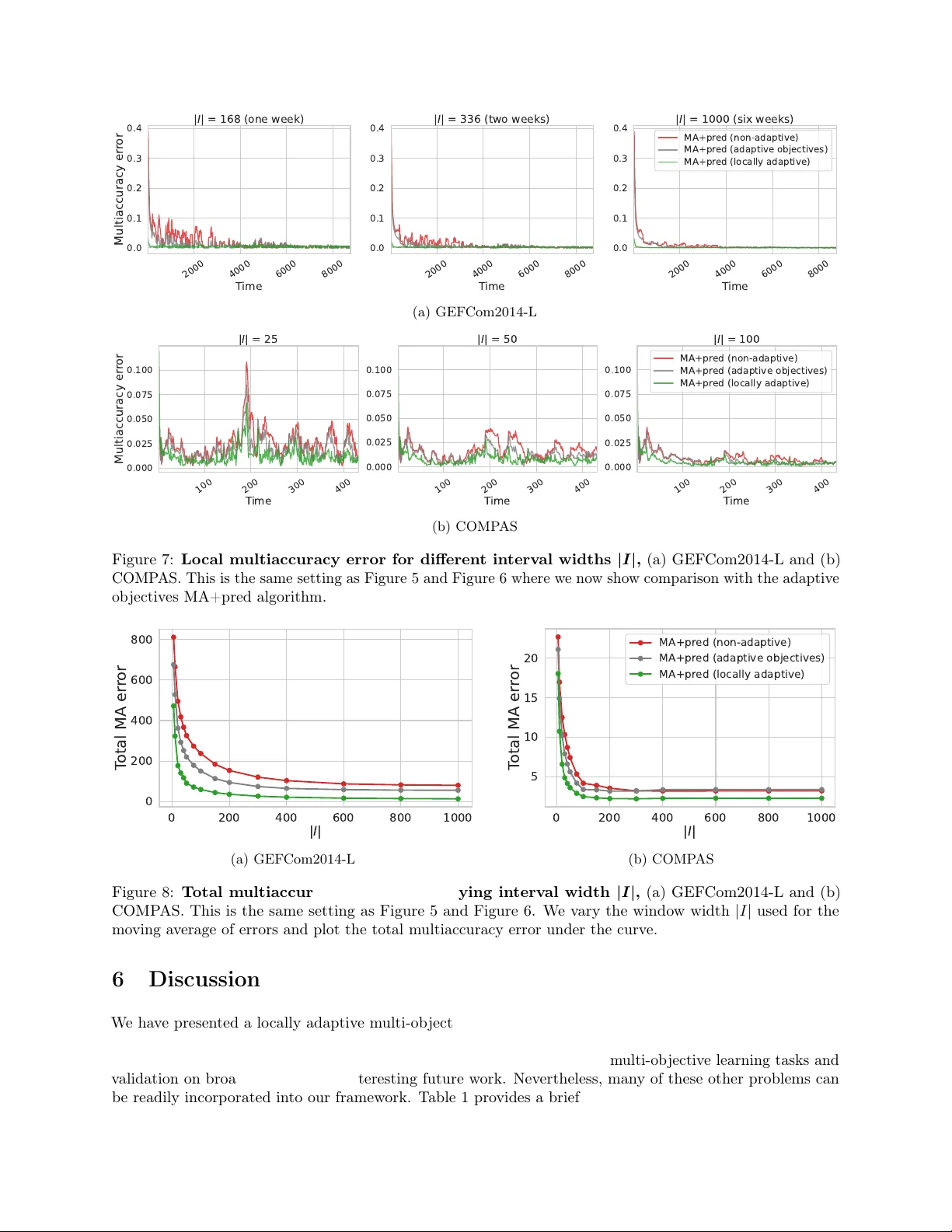
Loading comments...
Leave a Comment