On the Complexity of Offline Reinforcement Learning with $Q^\star$-Approximation and Partial Coverage

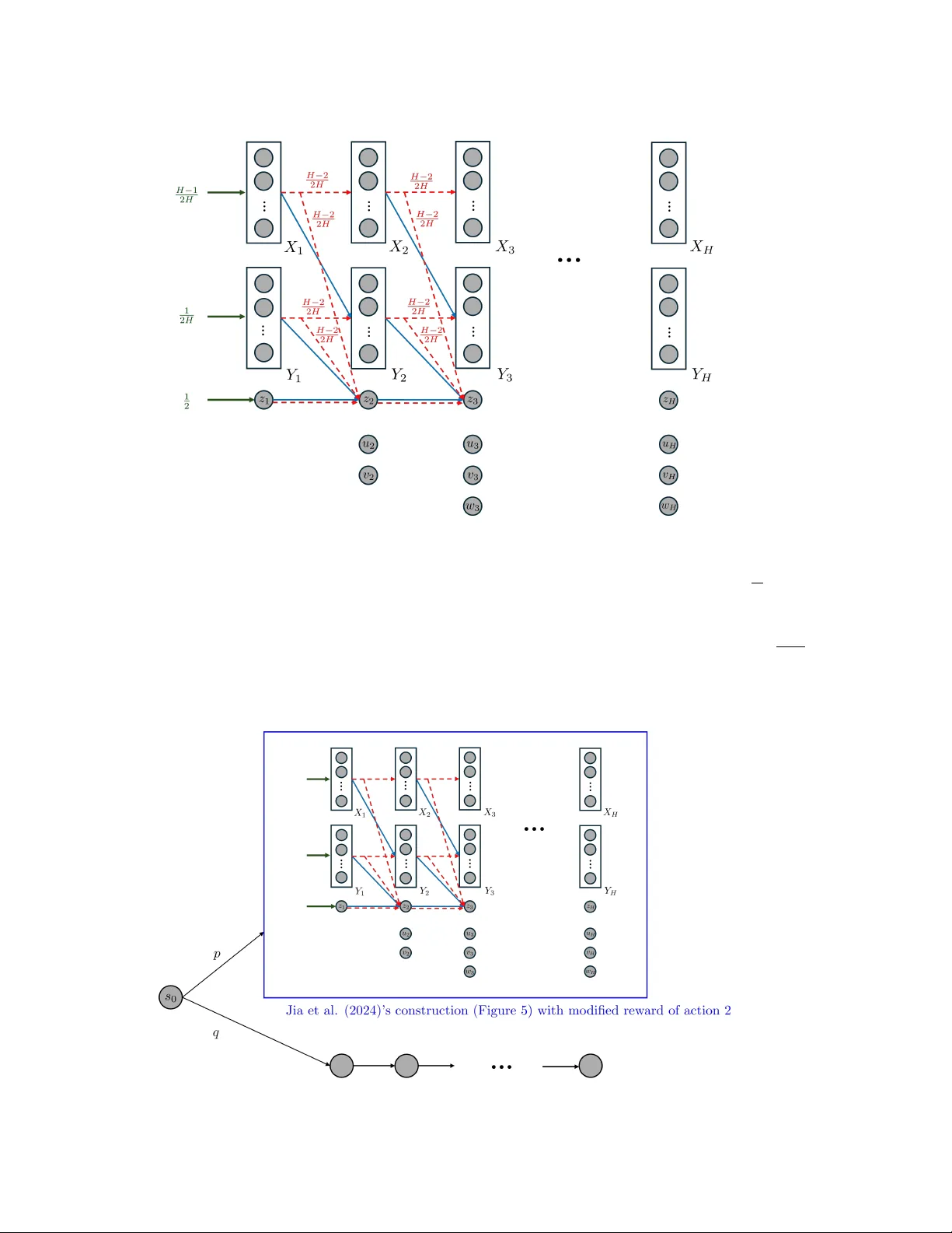
On the Complexity of Ofﬂine Reinf or cement Learning with Q ⋆ -A ppr oximation and Partial Cov erage Haolin Liu * S R S 8 R H @ V I R G I N I A . E D U Braham Snyder D Q R 2 Y E @ V I R G I N I A . E D U Chen-Y u W ei K F W 6 E N @ V I R G I N I A . E D U University of V irginia Abstract W e study of ﬂine reinforcement learning under Q ⋆ -approximation and partial cov erage, a setting that motiv ates practical algorithms such as Conservati ve Q -Learning (CQL) ( Kumar et al. , 2020 ) but has received limited theoretical attention. Our work is inspired by the following open ques- tion: Ar e Q ⋆ -r ealizability and Bellman completeness sufﬁcient for sample-efﬁcient of ﬂine RL under partial covera ge? W e answer this question in the negati ve by establishing an information-theoretic lower bound. Going substantially beyond this question, we introduce a general framew ork that characterizes the intrinsic complexity of a giv en Q ⋆ function class, drawing inspiration from model-free decision- estimation coef ﬁcients (DEC) for online RL ( Foster et al. , 2023b ; Liu et al. , 2025b ). This comple x- ity recov ers and improves the quantities underlying the guarantees of Chen and Jiang ( 2022 ) and Uehara et al. ( 2023 ), and extends to broader settings. Our decision-estimation decomposition can be combined with a wide range of Q ⋆ estimation procedures, greatly modularizing and generalizing existing approaches. Beyond the general framew ork, we make sev eral additional contributions: By de veloping a nov el second-order performance difference lemma, we obtain the ﬁrst ϵ − 2 sample complexity under partial coverage for soft Q -learning, improving the ϵ − 4 bound of Uehara et al. ( 2023 ). W e remove Chen and Jiang ( 2022 )’ s requirement for additional online interaction when the value gap of the true Q ⋆ function is unknown. W e also provide the ﬁrst characterization of ofﬂine learnability for general low-Bellman-rank MDPs without Bellman completeness ( Jiang et al. , 2017 ; Du et al. , 2021 ; Jin et al. , 2021 ), a canonical setting in online RL that remains unexplored in ofﬂine RL except for special cases. Finally , we provide the ﬁrst analysis for CQL under Q ⋆ -realizability and Bellman completeness beyond the tab ular case. 1. Introduction Of ﬂine Reinforcement Learning (RL) studies policy learning from a ﬁxed dataset, without interac- tion with the en vironment. This paradigm is appealing because it enables learning from data that may not have been generated by the learner itself. In practice, howe ver , it is rarely realistic to as- sume that the ofﬂine data covers the entire state-action space. In such partial covera ge settings, algorithms typically rely on pessimism to ensure safety against worst possible en vironments. Among value-based methods for ofﬂine RL with pessimism, two classes of algorithms are widely used: Q -learning-based methods such as Conserv ativ e Q -Learning (CQL) ( Kumar et al. , 2020 ), and actor-critic methods such as Behavior -Regularized Actor -Critic (BRA C) ( W u et al. , 2019 ). From a theoretical perspective, these methods are commonly analyzed under the Q ⋆ -realizability * Authors are listed in alphabetical order by last name. © H. Liu, B. Snyder & C.-Y . W ei. L I U S N Y D E R W E I and Q π -realizability assumptions, respectiv ely . For Q π -realizability settings, Xie et al. ( 2021 ) pro- vides a relati vely complete characterization of the sample complexity . For Q ⋆ -realizability settings, existing results ( Chen and Jiang , 2022 ; Uehara et al. , 2023 ) provide some characterizations. Their algorithms, howe ver , rely on estimating either the density ratio between the optimal policy and the data distrib ution or a certain Lagrange multiplier , which departs from the simple Q -learning used in practice. Moreov er , the analysis of Chen and Jiang ( 2022 ) hea vily relies on a v alue gap assumption, and that of Uehara et al. ( 2023 ) strongly depends on behavior regularization. The fundamental roles of these additional assumptions remain elusi ve. Our work is motiv ated by understanding the potential and limitations of ofﬂine RL under Q ⋆ - approximation and partial cov erage, with particular attention to explaining the simple and practi- cal CQL algorithm. More concretely , as the design of Q -learning is grounded in Bellman com- pleteness , a basic question arises: Ar e Q ⋆ -r ealizability and Bellman completeness suf ﬁcient for sample-efﬁcient ofﬂine RL under partial cover age? Though fundamental, this question has not been answered. The closest existing analyses are the upper bound by Chen and Jiang ( 2019 ), which addi- tionally requires full data cov erage, and the algorithm-dependent lo wer bound by Song et al. ( 2022 ), whose construction can actually be tackled by existing algorithms. In this work, we close the gap by pro viding an information-theoretic lo wer bound sho wing that the answer to the above question is ne gative in general. Howe ver , we go substantially beyond this. Inspired by the model-free decision-estimation coefﬁcient (DEC) frame work in online RL ( Foster et al. , 2023b ; Liu et al. , 2025b ), we decompose the learner’ s sub-optimality into decision complexity and estimation err or , where the decision complexity captures the sub-optimality in the worst possible environment consistent with the current estimate of Q ⋆ , and the estimation error quantiﬁes the inaccuracy of this estimate. The decision complexity not only improv es the value-gap bound in Chen and Jiang ( 2022 ), addressing its difﬁculty in hyper-parameter tuning, strengthens the results for soft Q -learning in Uehara et al. ( 2023 ), but also extends to broader settings. The estimation error can be controlled via various Q ⋆ estimation procedures—not only a verage Bellman error minimization under weight realizability ( Chen and Jiang , 2022 ; Uehara et al. , 2023 ), but also squared Bellman error minimization under Bellman completeness, which has not been established in of ﬂine RL under partial coverage. W e contribute to bridging online and ofﬂine RL theory , a direction advocated by Xie et al. ( 2023 ) and Amortila et al. ( 2024 ), who apply traditional ofﬂine RL techniques to online RL. In this work, we pursue the complementary direction. In online RL, while optimism is a general guiding princi- ple, it can be arbitrarily sub-optimal compared to information-directed methods in certain instances ( Lattimore and Szepesv ari , 2017 ). W e provide mirrored examples in ofﬂine RL, sho wing that value- based pessimism, though broadly applicable, can like wise be highly sub-optimal. Besides, we pro- vide the ﬁrst characterization of the ofﬂine learnability for MDPs with low Bellman rank without Bellman completeness ( Jiang et al. , 2017 ; Du et al. , 2021 ; Jin et al. , 2021 ). This is a canonical setting for online RL, but, to our knowledge, has ne ver been studied in ofﬂine RL except for special cases. Beyond Q ⋆ - and Q π -approximation, a line of work studies the partial coverage setting with density- ratio approximation ( Zhan et al. , 2022 ; Rashidinejad et al. , 2023 ; Ozdaglar et al. , 2023 ). Though our results for Q ⋆ -approximation do not directly apply there, our analytical framew ork provides a path to identifying a corresponding complexity notion in their setting. For ev en broader ofﬂine RL algorithms, we refer the reader to Che ( 2025 ) for a comprehensi ve re vie w and comparison. W e make several additional contributions of independent interest, including: 1) W e obtain the ﬁrst ϵ − 2 sample complexity bound for soft Q -learning (i.e., KL-regularized MDP) for ofﬂine RL 2 O FFL I N E R L W I T H Q ⋆ - A P P RO X I M A T I O N A N D P A RT I A L C OV E R A G E with partial coverage through the dev elopment of a novel second-or der performance differ ence lemma , and impro ve the guarantees in Uehara et al. ( 2023 ). 2) W e identify that double policy sampling and policy featur e coverag e are crucial for ofﬂine RL in low-Bellman-rank MDPs. These are restrictions that may not have been paid attention to in online RL. 3) W e giv e the ﬁrst analysis for the practical CQL algorithm beyond the tab ular-case analysis in ( K umar et al. , 2020 ). 2. Preliminary W e deal with both unregularized and regularized MDPs. For simplicity , we formulate regularized MDPs, while unregularized MDPs are just special cases when the re gularizer is zero. Regularized Markov Decision Processes W e consider a ﬁnite-horizon re gularized MDP deﬁned by M = ( S , A , P M , R M , s 1 , H, ψ ) , where S is the state space, A is the action space, P M : S × A → ∆( S ) is the transition function, R M : S × A → [0 , 1] is the re ward function, and ψ : ∆( A ) × S → R ≥ 0 is a state-dependent con vex regularizer for action distributions. W e assume a layered state space S , i.e., S = S 1 ∪ · · · ∪ S H where S h ∩ S h ′ = ∅ for an y h  = h ′ . Transitions only occur between adjacent layers: P M ( s ′ | s, a ) > 0 only if s ∈ S h and s ′ ∈ S h +1 . W ithout loss of generality , let S 1 = { s 1 } . A polic y π : S → ∆( A ) maps states to action distrib utions. Let Π be the set of policies. For any policy π , the regularized state v alue function is V π M ( s ) ≜ E π M  P H h ′ = h  R M ( s h ′ , a h ′ ) − ψ ( π ( ·| s h ′ ); s h ′ )    s h = s  for s ∈ S h , where E π M [ · ] denotes e xpectation ov er trajectories induced by π and P M . Furthermore, denote J M ( π ) ≜ V π M ( s 1 ) . By induction, the Bellman equations hold: Q π M ( s, a ) = R M ( s, a ) + I [ s / ∈ S H ] · E s ′ ∼ P M ( ·| s,a )  V π M ( s ′ )  , V π M ( s ) = E a ∼ π ( ·| s ) [ Q π M ( s, a )] − ψ ( π ( ·| s ); s ) . The optimal regularized value functions are Q ⋆ M ( s, a ) = max π Q π M ( s, a ) and V ⋆ M ( s ) = max π V π M ( s ) , and the optimal policy is π M ∈ argmax π J M ( π ) . 1 The Bellman optimality equations hold: Q ⋆ M ( s, a ) = R M ( s, a ) + I [ s / ∈ S H ] · E s ′ ∼ P M ( ·| s,a )  V ⋆ M ( s ′ )  , V ⋆ M ( s ) = max p ∈ ∆( A )  E a ∼ p [ Q ⋆ M ( s, a )] − ψ ( p ; s )  , π M ( · | s ) ∈ argmax p ∈ ∆( A )  E a ∼ p [ Q ⋆ M ( s, a )] − ψ ( p ; s )  . For a policy π , denote the state occupancy measure as d π M ( s ) ≜ E π M [ I { s h = s } ] for s ∈ S h , and the state-action occupancy measure as d π M ( s, a ) ≜ d π M ( s ) π ( a | s ) . Though d π M is not a distribution as P s ∈S d π M ( s ) = H , we denote E s ∼ d π [ g ( s )] ≜ P s d π ( s ) g ( s ) for any function g . Assume the true en vironment follo ws MDP M ⋆ = ( S , A , P , R, s 1 , H , ψ ) , and for simplicity , we write V π ( s ) ≜ V π M ⋆ ( s ) , Q π ( s, a ) ≜ Q π M ⋆ ( s, a ) , V ⋆ ( s ) ≜ V ⋆ M ⋆ ( s ) , Q ⋆ ( s, a ) ≜ Q ⋆ M ⋆ ( s, a ) , J ( π ) ≜ J M ⋆ ( π ) , π ⋆ ≜ π M ⋆ , and d π ≜ d π M ⋆ . Ofﬂine Reinfor cement Learning In ofﬂine RL, the learner only has access to a pre-collected dataset D from MDP M ⋆ and cannot interact with the environment. The dataset D consists of n i.i.d. tuples ( s, a, r, s ′ ) , where ( s, a ) ∼ µ for some unkno wn distribution µ ∈ ∆( S × A ) , E [ r | s, a ] = R ( s, a ) , and s ′ ∼ P ( ·| s, a ) . The goal is to learn a policy ˆ π that minimizes the sub-optimality relativ e 1. W e let π M = ( π M ( ·| s )) s ∈S be an arbitrary optimal polic y when multiple optimal policies e xist. All our results hold for any tie-breaking rule. In other words, for upper bounds we adopt the worst tie-breaking for the learner , and for lower bounds the best tie-breaking. The same con vention applies to π f deﬁned later . 3 L I U S N Y D E R W E I to the optimal policy π ⋆ , namely J ( π ⋆ ) − J ( ˆ π ) . W e seek cover age-adaptive performance, where the sub-optimality adapts to the degree to which µ covers π ⋆ . The standard coverage is deﬁned as: Deﬁnition 1 (Coverage) F or any policy π , deﬁne C π = max ( s,a ) ∈S ×A d π ( s,a ) H µ ( s,a ) . 2 In value-based of ﬂine RL, function approximation is used to approximate value functions. In this paper , we focus on the Q ⋆ -approximation scheme and assume Q ⋆ -realizability: Deﬁnition 2 ( Q ⋆ -realizability) The learner has access to a function class F ⊂ { f : S × A → R } such that Q ⋆ ∈ F . F or any f ∈ F , denote f ( s ) = max p ∈ ∆( A )  E a ∼ p [ f ( s, a )] − ψ ( p ; s )  and denote π f ( · | s ) = argmax p ∈ ∆( A )  E a ∼ p [ f ( s, a )] − ψ ( p ; s )  with arbitrary tie-br eaking. Bellman Operator Deﬁne the Bellman operator T as [ T f ]( s, a ) = R ( s, a ) + E s ′ ∼ P ( ·| s,a ) [ f ( s ′ )] = R ( s, a ) + E s ′ ∼ P ( ·| s,a ) [ E a ′ ∼ π f ( ·| s ′ ) f ( s ′ , a ′ ) − ψ ( π f ; s ′ )] . Regularizer For con ve x function Φ : ∆( A ) → R , let Breg Φ ( x, y ) ≜ Φ ( x ) − Φ ( y ) −⟨∇ Φ ( y ) , x − y ⟩ be the Bregman diver gence deﬁned with Φ . W e write Breg ψ ( x, y ; s ) ≜ Breg ψ ( · ; s ) ( x, y ) for any x, y ∈ ∆( A ) and Breg ψ ( π , π ′ ; s ) ≜ Breg ψ ( · ; s ) ( π ( ·| s ) , π ′ ( ·| s )) for any policies π , π ′ . W e focus on regularizer ψ ( p ; s ) = α Breg Φ ( p ; π ref ( ·| s )) where Φ is a con ve x function, π ref is a giv en reference policy , and α ≥ 0 is the weight of re gularization. W e also write ψ ( π ( ·| s ); s ) ≜ ψ ( π ; s ) . 3. An Information-Theor etic Lower Bound W e start with an information-theoretic lower bound that shows the hardness of of ﬂine RL under partial cov erage, with only Q ⋆ -realizability and Bellman completeness (deﬁned belo w). Assumption 1 (Bellman completeness) Along with the F in Deﬁnition 2 , the learner has access to a function class G ⊂ { g : S × A → R } such that [ T f ] ∈ G for any f ∈ F . Theorem 1 There exists a family of MDPs M , a function class F with |F | = 4 , and an ofﬂine data distribution µ such that under any true model M ⋆ ∈ M , Q ⋆ -r ealizability and Bellman completeness hold (with G = F ), and has covera ge C π ⋆ = Θ(1) . However , to achie ve E [ J ( π ⋆ ) − J ( ˆ π )] ≤ ϵ with M ⋆ ∼ Unif ( M ) , the learner must access n ≥ Ω  1 ϵ min  p |S | , 1 ∆ 2  ofﬂine samples, wher e ∆ = min s ( V ⋆ ( s ) − max a  = π ⋆ ( s ) Q ⋆ ( s, a )) is a par ameter which can be chosen arbitrarily in [0 , 1 4 ] . Even if the learner can access trajectory feedback ( s 1 , a 1 , r 1 , · · · , s H , a H , r H ) fr om an ofﬂine policy π b such that max s,a d π ⋆ ( s,a ) d π b ( s,a ) = Θ(1) , n ≥ Ω  1 ϵ poly( H ) min { 2 H , p |S | , 1 ∆ 2 }  trajectories ar e still needed. While the w ork of Song et al. ( 2022 ) mak es a similar claim, their lo wer bound is algorithm-speciﬁc and relies on a tie-breaking rule against the learner . Their construction is actually a simple three- state MDP that can be handled by existing algorithms. In contrast, our lower bound is information- theoretic, and holds without any tie-breaking. Below , we describe the construction. W e start by obtaining a lo wer bound of min { p |S | , 1 ∆ 2 } without the ϵ − 1 factor ( Lemma 16 ). The construction relies on confusing the learner with the four families of MDPs sho wn in Figure 2 , from which M ⋆ is uniformly drawn. On the initial state s 1 , two actions u and v giv e either Ber ( 1 2 ) or Ber ( 1 2 + ∆) rew ard (depending on M ⋆ ). The action that has Ber ( 1 2 ) re ward leads to the next 2. The division by H is to correct the mismatch between P s,a d π ( s, a ) = H and P s,a µ ( s, a ) = 1 . 4 O FFL I N E R L W I T H Q ⋆ - A P P RO X I M A T I O N A N D P A RT I A L C OV E R A G E state uniformly drawn from the group W A , while the other leads to states uniformly from group W B . From W A and W B , taking the unique action a leads to s A and s B respecti vely , with 0 re ward. Finally , on s A or s B , three actions give deterministic rew ard as speciﬁed in Figure 2 . Clearly , the optimal policy π ⋆ is the one that chooses the Ber ( 1 2 + ∆) action and chooses z on s B . The function set F with |F | = 4 that satisﬁes realizability and Bellman completeness are giv en in Appendix A.2 . The ofﬂine distribution µ is induced by a behavior policy that chooses { u, v } uniformly on s 1 , and chooses z on s A and s B . This covers the optimal policy with C π ⋆ ≤ 2 . As the learner only observes ( s, a, r , s ′ ) but not trajectories, what the learner sees are the following three types of samples: T ype 1 : ( s 1 , a 1 , r 1 , w 1 ) where a 1 ∼ Unif ( { u, v } ) , r 1 ∈ { 0 , 1 } , w 1 ∈ W A ∪ W B , T ype 2 : ( w 2 , a, 0 , s 2 ) where w 2 ∼ Unif ( W A ∪ W B ) and s 2 ∈ { s A , s B } , and T ype 3 : ( s 3 , z , r 3 ) where s 3 ∼ Unif ( { s A , s B } ) and r 3 ∈ { 0 , 1 } . Belo w , we argue that while the optimal policy has an expected rew ard of 1 2 + ∆ + 1 , it is hard for the learner to output a policy ˆ π that achie ves an expected reward of 1 2 + ∆ 2 + 1 2 unless n ≳ min { √ m, 1 / ∆ 2 } , where | W A | = | W B | = m . Intuition for n ≥ Ω(min { p |S | , 1 / ∆ 2 } ) lower bound Since the optimal policy goes to W B , a goal of the learner is to distinguish whether it is u or v that leads to W B . T ype 1 data could re veal this information as the action to W B has a higher expected re ward of 1 2 + ∆ . Howe ver , this requires Ω( 1 ∆ 2 ) samples. The learner might also try to tell them apart by the next state w 1 after choosing u and v ; howe ver , by the construction of the function set F , for all f ∈ F and w ∈ W A ∪ W B , the v alue f ( w , a ) = 1 is the same, and thus the learner cannot tell whether w 1 comes from W A or W B based on the function set (in Appendix A.1 we formally treat this by including in each family all possible assignments from state to { W A , W B } , a technique similar to that of Foster et al. ( 2022 ) and Jia et al. ( 2024 )). Finally , the learner might also le verage T ype 2 data—indeed, for a T ype 2 sample ( w 2 , a, 0 , s 2 ) , the learner can tell whether w 2 ∈ W A or w 2 ∈ W B based on the identity of s 2 ; ho wev er , as long as | W A | and | W B | are large enough, the learner ne ver sees the same state from W A and W B twice, and thus the information re vealed from T ype 2 does not help determine whether w 1 in T ype 1 is from W A or W B . Also, on s A or s B , the learner’ s output policy ˆ π should not choose x or y : choosing either of them is risky because the of ﬂine data ne ver observ es x or y and one of them will lead to − 2 reward. Overall, it is hard for the learner to determine between u and v , and the learner should only choose z on s A and s B . A random guess between u and v can only achieve an expected re ward of 1 2 + ∆ 2 + 1 2 , which has a gap of 1 2 + ∆ 2 = Θ(1) compared with π ⋆ . In Theorem 1 , we strengthen the above construction to obtain ϵ -dependent and trajectory- feedback lo wer bounds (see Appendix A ). W e note that our gap-dependent lower bound is quite dif ferent from those in online RL or simpler ofﬂine RL settings ( W ang et al. , 2022 ; Nguyen-T ang et al. , 2023 ). In those settings, if the learner cannot tell apart two actions with gap ∆ , the sub- optimality suffered is only of order ∆ . In our case, before the learner tells apart two actions of gap ∆ , the learner suffers Θ(1) sub-optimality . This difference also shows in the sample complexity bounds: in prior settings, the learner can achiev e O ( 1 ϵ 2 ) sample complexity regardless of the value gap. In contrast, the sample complexity in Theorem 1 scales with 1 ϵ ∆ 2 , which can become arbitrarily large e ven under constant ϵ . W e remark that when F is the linear function class with a known feature mapping, polynomial sample complexity without dependence on ∆ is possible under partial coverage and Bellman com- 5 L I U S N Y D E R W E I Algorithm 1 Greedy Decision from Estimation ( G D E) Input: Conﬁdence set F conf . Compute ˆ f ∈ argmin f ∈F conf f ( s 1 ) . Output: ˆ π = π ˆ f . pleteness ( Golowich and Moitra , 2024 ). Their result heavily relies on the linear structure. It is an interesting direction to unify the linear and non-linear results. 4. How to Make Decisions fr om Estimations in Ofﬂine Reinfor cement Learning? In ofﬂine RL with Q ⋆ -realizability , the ofﬂine dataset induces a conﬁdence set F conf of plausible Q ⋆ functions. Then the learner must select a policy ˆ π , with performance measured by J ( π ⋆ ) − J ( ˆ π ) . This section assumes the learner has already constructed F conf and focuses on deriving ˆ π from it. In Appendix B , we discuss the case of bounding J ( ˚ π ) − J ( ˆ π ) with an arbitrary comparator ˚ π  = π ⋆ . 4.1. A T ale of T wo P essimism Principles W e identify two distinct pessimism principles in prior work to deri ve a policy from the conﬁ- dence set. The ﬁrst, which we refer to as policy-centric pessimism , has been adopted in model- approximation ( Uehara and Sun , 2021 ) and Q π -approximation schemes ( Xie et al. , 2021 ). This approach aligns with the r obust optimization principle ( Gorissen et al. , 2015 ), where the learner outputs a policy ˆ π that maximizes the worst-case performance over the uncertainty set of models: ˆ π = argmax π min M ∈M conf J M ( π ) (1) Ho wev er , prior work on Q ⋆ -approximation often follows a different principle, which we call value-centric pessimism . Under this principle, the order between min M and max π are swapped: ˆ M = argmin M ∈M conf max π J M ( π ) , then let ˆ π = π ˆ M . (2) For example, this is the core idea of Chen and Jiang ( 2022 ), which we present in Algorithm 1 . Note that Algorithm 1 and (2) are equi valent: with a conﬁdence set F conf for Q ⋆ , we can de- ﬁne a conﬁdence set for M ⋆ : M conf = { M : Q ⋆ M ∈ F conf } . Thus, min f ∈F conf f ( s 1 ) = min M ∈M conf V ⋆ M ( s 1 ) = min M ∈M conf max π J M ( π ) . Uehara et al. ( 2023 )’ s algorithm is slightly dif ferent, but it also ﬁrst estimates ˆ f and then outputs ˆ π = π ˆ f . The deviation of Q ⋆ -approximation from robust optimization is not surprising: in model- or Q π - approximation, the learner can ev aluate J M ( π ) for any π by querying the model or Q π set. In Q ⋆ - approximation, howe ver , J M ( π ) for a ﬁxed π may not be represented by any function in F conf unless π = π M . This forces the algorithm to treat J M ( π M ) = max π J M ( π ) as an inseparable unit as in (2) . Ho wev er , this pessimism sometimes produces less desirable decision, as in the example belo w . Example 1 Assume a single state s 1 and two actions x, y . Let F conf = { f x , f y } with f x ( s 1 , x ) = 1 , f x ( s 1 , y ) = 0 , f y ( s 1 , x ) = 1 2 − ∆ , f y ( s 1 , y ) = 1 2 + ∆ for some ∆ ∈ (0 , 0 . 01] . P olicy-centric pes- simism (1) chooses action argmax a min f ∈{ f x ,f y } f ( s 1 , a ) = x . V alue-centric pessimism (2) chooses function argmin f ∈{ f x ,f y } max a f ( s 1 , a ) = f y and then chooses action argmax a f y ( s 1 , a ) = y . 6 O FFL I N E R L W I T H Q ⋆ - A P P RO X I M A T I O N A N D P A RT I A L C OV E R A G E Online model-based DEC: min ρ ∈ ∆(Π) max M ∈M E π ∼ ρ h J M ( π M ) − J M ( π ) − γ E M ∼ p osterio r [ D π ( M ∥ M )] i Online model-free DEC: min ρ ∈ ∆(Π) max M ∈M E π ∼ ρ h J M ( π M ) − J M ( π ) − γ E f ∼ p osterio r [ D π ( f ∥ M )] i Of ﬂine model-free DEC: min ρ ∈ ∆(Π) max M ∈M conf E π ∼ ρ h J M ( π M ) − J M ( π ) − γ max f ∈F conf D π M ( f ∥ M ) i Figure 1: Comparison of DEC objectiv es in online and of ﬂine settings for a giv en discrepanc y measure D . If the true envir onment is described by f x , then the sub-optimality of policy-centric pessimism and value-centric pessimism is 0 and 1 , respectively; if the true en vir onment is described by f y , then their sub-optimality is 2∆ ≤ 0 . 02 and 0 , r espectively . In this scenario, policy-centric pessimism sacriﬁces a negligible 2∆ in one world to av oid a catas- trophic error (gap of 1 ) in the other —a robust beha vior we usually fa vor in of ﬂine RL. Can we design an algorithm under the Q ⋆ -approximation that makes policy-centric decisions to ensure rob ustness? In the next subsection, we answer this afﬁrmati vely . The frame work we de velop draws inspiration from the model-fr ee decision-estimation coefﬁcient (DEC) ( Foster et al. , 2023b ; Liu et al. , 2025a , b ) which optimizes the learner’ s decision with the help of the induced model set (the M conf abov e), without incurring statistical cost that scales with the size of the model set. 4.2. A Decision-Estimation Coefﬁcient for Ofﬂine RL under Partial Co verage W e aim for a principled way to design of ﬂine RL algorithms. W e ﬁrst revie w ideas in the existing online DEC framew ork. In model-based DEC ( Foster et al. , 2021 , 2023a ; Xu and Zeevi , 2023 ), the learner seeks a policy that minimizes regret against an adversarially chosen model (hence aligned with robust optimization). Howe ver , this model must remain close—measured under the learner’ s current policy—to the posterior of M ⋆ estimated from collected data. T o achiev e this, ev ery model is penalized according to its discrepancy from the model posterior . This corresponds to the ﬁrst decision rule in Figure 1 . Model-free DEC ( Foster et al. , 2023b ; Liu et al. , 2025b ) follo ws a similar principle, b ut instead of maintaining a posterior of M ⋆ , it maintains a posterior of Q ⋆ . The learner’ s policy is optimized against the induced model set M = { Q ⋆ M ∈ F } . This giv es the second decision rule in Figure 1 . In of ﬂine RL, the Q ⋆ conﬁdence set plays a similar role as the Q ⋆ posterior in the online setting. Similarly , the learner seeks a policy that minimizes the sub-optimality against an adv ersarial model that remains close to the conﬁdence set. A ke y dif ference is that now this closeness is measured under each model’ s own optimal policy . For one, the learner’ s policy can no longer help detecting the discrepancy between a model and Q ⋆ posterior as in the online case, so they should not optimize their policy o ver it. For another , this has the ef fect of penalizing models whose optimal policies are poorly cov ered, hence achieving co verage-adapti ve guarantee. T o measure the closeness between a model M and a conﬁdence function set under policy π M , we use max f ∈F conf D π M ( f ∥ M ) with standard discrepancy functions D such as the Bellman error (will be clariﬁed in Sec tion 5 ). The intuition is that for the true model M ⋆ , max f ∈F conf D π ⋆ ( f ∥ M ⋆ ) is e xpected to be small (usually of order C π ⋆ /n where n is the number of of ﬂine samples), as any function f that deviates signiﬁcantly from M ⋆ should hav e already been excluded from the 7 L I U S N Y D E R W E I Algorithm 2 Of ﬂine Robust Estimation-to-Decision (E 2 D . O R ) Input: Conﬁdence set F conf , di ver gence measure D π ( f ∥ M ) , parameter γ for the of fset version. Deﬁne M conf = { M : Q ⋆ M ∈ F conf } and compute ˆ ρ =            argmin ρ ∈ ∆(Π) max M ∈M conf E π ∼ ρ  J M ( π M ) − J M ( π ) − γ max f ∈F conf D π M ( f ∥ M )  (of fset version) argmin ρ ∈ ∆(Π) max M ∈M conf J M ( π M ) − E π ∼ ρ [ J M ( π )] (max f ∈F conf D π M ( f ∥ M )) 1 / 2 . (ratio version) Output: mixture policy ˆ π ∼ ˆ ρ . conﬁdence set F conf . This maximum discrepancy provides maximal power of discrimination. This gi ves to the third decision rule in Figure 1 . This motiv ates the design of E 2 D . O R ( Algorithm 2 ). W e provide two versions of it, different in the way of trading the sub-optimality term and the discrepancy term. The of fset version aligns with online DEC, and could gi ve a better bound when the discrepancy term may approach zero. The ratio version, ho wev er , can better handle the case where C π ⋆ is unkno wn. Deﬁne the follo wing two complexities (Of ﬂine Rob ust DEC) that naturally arise from the algorithm: Ordec - O D γ ( F conf ) := min ρ ∈ ∆(Π) max M ∈M conf E π ∼ ρ h J M ( π M ) − J M ( π ) − γ max f ∈F conf D π M ( f ∥ M ) i , (3) Ordec - R D ( F conf ) := min ρ ∈ ∆(Π) max M ∈M conf J M ( π M ) − E π ∼ ρ [ J M ( π )] (max f ∈F conf D π M ( f ∥ M )) 1 / 2 . (4) It holds that Ordec - O D γ ( F conf ) ≤ 4 γ  Ordec - R D ( F conf )  2 ( Lemma 17 ). W ith them, we hav e: Theorem 2 If Q ⋆ ∈ F conf , then E 2 D . O R ensures (of fset version) J ( π ⋆ ) − E [ J ( ˆ π )] ≤ Ordec - O D γ ( F conf ) + γ max f ∈F conf D π ⋆ ( f ∥ M ⋆ ) , (ratio version) J ( π ⋆ ) − E [ J ( ˆ π )] ≤ Ordec - R D ( F conf )  max f ∈F conf D π ⋆ ( f ∥ M ⋆ )  1 / 2 . See Appendix C for the proof. 4.3. Comparison with V alue-Centric Pessimism W e may express the bound of G D E ( Algorithm 1 ) using similar quantities as (4) . Deﬁne Gdec D ( F conf ) := max M ∈M conf J M ( π M ) − J M ( π ˆ f )  D π M ( ˆ f ∥ M )  1 / 2 , (5) where ˆ f = argmin f ∈F conf f ( s 1 ) . Clearly , it holds that Ordec - R D ≤ Gdec D . The guarantee of G D E ( Algorithm 1 ) is giv en by Theorem 3 If Q ⋆ ∈ F conf , then G D E ensur es J ( π ⋆ ) − J ( ˆ π ) ≤ Gdec D ( F conf )  D π ⋆ ( ˆ f ∥ M ⋆ )  1 / 2 . 8 O FFL I N E R L W I T H Q ⋆ - A P P RO X I M A T I O N A N D P A RT I A L C OV E R A G E See Appendix C for the proof. Comparing Ordec (3)(4) and Gdec (5) , it is clear that the ben- eﬁt of E 2 D . O R ov er G D E is the additional optimization over ρ and f that reduces the bound in the worst-case en vironment. G D E seems to admit a smaller div ergence term D π ⋆ ( ˆ f ∥ M ⋆ ) ≤ max f ∈F conf D π ⋆ ( f ∥ M ⋆ ) , but as the learner has no control over D π ⋆ ( ˆ f ∥ M ⋆ ) , it can only be bounded by the worst case in all analysis. In the following sections, we bound Ordec ( Section 5 ) and max f ∈F conf D π ⋆ ( f ∥ M ⋆ ) ( Section 6 ) in dif ferent scenarios. 5. Bounding Ofﬂine Robust DEC In this section, we provide examples where Ordec is bounded. As the lower bound in Section 3 sho ws, Q ⋆ -approximation with partial cov erage is a challenging or ev en impossible regime, espe- cially when the optimal value function has a v ery small or zero value g ap. Therefore, even with the more reﬁned decision principle developed in Section 4 , some form of gap conditions or assumptions on the uniqueness of the optimal action is unav oidable. Throughout this section, we consider the av erage Bellman error: D π av ( f ∥ M ) =  E ( s,a ) ∼ d π M  f ( s, a ) − R M ( s, a ) − E s ′ ∼ P M ( ·| s,a )  f ( s ′ )   2 . (6) W e denote Ordec - O av γ for Ordec - O D av γ (and similar for others). T o connect Ordec with comple xities established in prior work, we deﬁne the Exploitability Ratio : Deﬁnition 3 (Exploitability Ratio) F or f ∈ F conf , deﬁne ER ( f ; F conf ) = max M ∈M conf J M ( π M ) − J M ( π f ) E ( s,a ) ∼ d π M M [ f ( s ) − f ( s, a ) + ψ ( π M ; s )] with 0 0 ≜ 0 . If π f or π M is not unique, c hoose the one that makes this ratio the lar gest. The ratio ER ( f ; F conf ) quantiﬁes ho w much the greedy policy π f may be exploited by another model M ∈ M conf (i.e., J M ( π M ) − J M ( π f ) in the numerator), relati ve to ho w much f thinks π f is better than π M (i.e., f ( s ) − f ( s, π M ( s )) + ψ ( π M ; s ) in the denominator). The next theorem sho ws performance bounds achie ved by E 2 D . O R and G D E in terms of ER : Theorem 4 Let ˆ f = argmin f ∈F conf f ( s 1 ) and assume Q ⋆ ∈ F conf . Then the following hold: Ordec - O av γ ( F conf ) ≤ 1 2 γ ER ( Q ⋆ ; F conf ) 2 + γ max f ∈F conf D π ⋆ av ( f ∥ M ⋆ ) , (7) Ordec - R av ( F conf ) ≤ ER ( ˆ f ; F conf ) , (8) Gdec av ( F conf ) ≤ ER ( ˆ f ; F conf ) . (9) In the next tw o subsections, we consider unregularized MDPs and regularzied MDPs, respecti vely . 5.1. Unregularized Case ( ψ ≡ 0 ) When ψ ≡ 0 , ER in Deﬁnition 3 recover the gap bound in Chen and Jiang ( 2022 ): Theorem 5 Let ∆ f ≜ min s  f ( s, π f ( s )) − max a  = π f ( s ) f ( s, a )  . Then for any f ∈ F conf , it holds that ER ( f ; F conf ) ≤ H / ∆ f . 9 L I U S N Y D E R W E I Comparing E 2 D . O R (offset) with ( E 2 D . O R (ratio) or G D E ) Assuming Bellman complete- ness, we ha ve max f ∈F conf D π ⋆ av ( f ∥ M ⋆ ) ≲ H 3 C π ⋆ /n (omitting log factors) ( Section 6.1 ). Combin- ing Theorem 4 , Theorem 5 with Theorem 2 , Theorem 3 , we get sub-optimality bounds: E 2 D . O R (offset): J ( π ⋆ ) − E [ J ( ˆ π )] ≲ H 2 γ ∆ 2 Q ⋆ + γ H 3 C π ⋆ n =  1 ∆ 2 Q ⋆ + C π ⋆  H 5 2 √ n (10) E 2 D . O R (ratio) or G D E : J ( π ⋆ ) − E [ J ( ˆ π )] ≲ H 5 2 ∆ ˆ f r C π ⋆ n (11) where ˆ f := argmin f ∈F conf f ( s 1 ) and we choose γ = p n/H in E 2 D . O R (of fset). A salient property of E 2 D . O R (of fset) is that the bound automatically adapts to the true v alue gap ∆ Q ⋆ without any prior knowledge of it. This addresses the restriction of Chen and Jiang ( 2022 ) that requires ∆ Q ⋆ as an input to the algorithm. A price is that its γ can only be tuned sub-optimally with respect to C π ⋆ . In contrast, E 2 D . O R (ratio) and G D E hav e optimal dependence on C π ⋆ , but incur the ∆ − 1 ˆ f factor , which is not controllable and could be much larger than ∆ − 1 Q ⋆ . W e argue that scaling with ER ( Q ⋆ ; F conf ) (or ∆ − 1 Q ⋆ ) is more desirable than ER ( ˆ f ; F conf ) (or ∆ − 1 ˆ f ). Observe that whene ver F ′ conf ⊂ F conf , we have ER ( Q ⋆ ; F ′ conf ) ≤ ER ( Q ⋆ ; F conf ) . Hence, the ﬁrst term in (7) always improves as F conf shrinks. In contrast, as ˆ f changes with F conf , ER ( ˆ f ; F conf ) has no such monotonic improv ement property . Comparing ( E 2 D . O R (offset) or E 2 D . O R (ratio) ) with G D E E 2 D . O R gains beneﬁts with the min ρ ∈ ∆(Π) operator in av oiding risks. This can be observed from the simple e xample below . Example 2 Consider the case with a single state s 1 and thr ee actions x, y , z . Let F conf = { f x , f y } with f x ( s 1 , x ) = 1 , f x ( s 1 , y ) = 0 , f x ( s 1 , z ) = 1 − ∆ and f y ( s 1 , x ) = 0 , f y ( s 1 , y ) = 1 , f y ( s 1 , z ) = 1 − ∆ for some 0 < ∆ ≤ 0 . 01 . It can be veriﬁed that Ordec - O av γ ( F conf ) ≤ ∆ − γ , Ordec - R av ( F conf ) ≤ ∆ , and Gdec av ( F conf ) = 1 . In Example 2 , it is clear that choosing x or y is risky; choosing z , while always being sub-optimal, is the safest choice, and that is exactly the decision that will be made by E 2 D . O R . Overall, E 2 D . O R gains multiple beneﬁts over G D E due to the additional optimization over f and ρ in Algorithm 2 . The beneﬁts might not fully show in the upper bounds in Theorem 4 , (10) , and (11) , because those bounds are essentially obtained by plugging in speciﬁc choices of f or ρ , and in speciﬁc instances the algorithm may ﬁnd e ven better f and ρ . W e notice that Song et al. ( 2022 ) and Uehara et al. ( 2023 ) raise concerns on the applicability of the gap assumption ( Chen and Jiang , 2022 ) in continuous action space. Our complexities ( (3) , (4) , Deﬁnition 3 ) poses no requirement for discrete actions or strict value gaps. Below is a continuous- action example with bounded Ordec : Theorem 6 Consider the linear setting with given featur e mapping ϕ : S × A → R d . Assume 1) there exists θ ⋆ ∈ R d such that Q ⋆ ( s, a ) = ϕ ( s, a ) ⊤ θ ⋆ , 2) for any policy π and any action pair a, b ∈ A , | Q π ( s, a ) − Q π ( s, b ) | ≤ L ∥ ϕ ( s, a ) − ϕ ( s, b ) ∥ , and 3) for all s , ϕ ( s, · ) ⊂ R d is a set with the following pr operty: for some κ > 0 , β ≥ 1 (denote π ⋆ ( s ) = argmax a ϕ ( s, a ) ⊤ θ ⋆ ): ∀ a ( ϕ ( s, π ⋆ ( s )) − ϕ ( s , a )) ⊤ θ ⋆ ≥ κ ∥ ϕ ( s, π ⋆ ( s )) − ϕ ( s , a ) ∥ β . (12) Then Ordec - O av γ ( F conf ) ≤ O   γ − 1 κ − 2 L 2 β  1 2 β − 1  + γ max f ∈F conf D π ⋆ av ( f ∥ M ⋆ ) . 10 O FFL I N E R L W I T H Q ⋆ - A P P RO X I M A T I O N A N D P A RT I A L C OV E R A G E The ﬁrst two assumptions in Theorem 6 are mild. The third (12) requires some curvatur e at the boundary of the feature set, making the optimal action unique. Notably , it only requires curv ature at the greedy action of θ ⋆ but not other θ ’ s, similar to (10) that only depends on the value gap of Q ⋆ . 5.2. Regularized Case ( ψ ≡ 0 ) Besides value gaps ( Theorem 5 ) and decision sets with curvature ( Theorem 6 ), another setting that guarantees a unique optimal action is regularization with a strictly con ve x function. In this subsec- tion, we provide guarantees under a rich family of re gularization with Legendre functions satisfying Assumption 2 , which includes the Bregman div ergence induced by (negati ve) Shannon entropy , Tsallis entropy , and log-barrier as special cases ( Lemma 7 ). This recov ers the standard KL regular- ization of the form ψ ( p ; s ) = α KL ( p, π ref ( ·| s )) studied in, e.g., Uehara et al. ( 2023 ). Assumption 2 The re gularizer ψ satisﬁes the following conditions with constants C ψ 1 , C ψ 2 > 0 : 1. ψ ( · ; s ) is a Le gendr e function ( Deﬁnition 6 ) for any s . 2. C ψ 1 Breg ψ ( π f 1 , π f 2 ; s ) ≥ Breg ψ ( π f 2 , π f 1 ; s ) for any f 1 , f 2 ∈ F and s ∈ S . 3. C ψ 2 Breg ψ ( π f 1 , π f 2 ; s ) ≥ KL ( π f 1 ( ·| s ) ∥ π f 2 ( ·| s )) for any f 1 , f 2 ∈ F and s ∈ S . Lemma 7 Let ψ ( p ; s ) = α Breg Φ ( p, π ref ( ·| s )) for some r efer ence policy π ref . The following choices of Φ make Assumption 2 hold with r espective ( C ψ 1 , C ψ 2 ) : • Φ ( p ) = P a ∈A p ( a ) log ( p ( a )) (Shannon entropy): ( C ψ 1 , C ψ 2 ) = (1 + 4 H α , 1 α ) . • Φ ( p ) = 1 1 − q (1 − P a p ( a ) q ) with q ∈ (0 , 1) (Tsallis entropy): ( C ψ 1 , C ψ 2 ) =  1 + 2 H (1 − q ) αq  2 − q 1 − q , 1 αq  . • Φ ( p ) = − P a ∈A log ( p ( a )) (log-barrier): ( C ψ 1 , C ψ 2 ) = (1 + 2 H α , 2 α ) . W ith Assumption 2 , the exploitability ratios can be controlled as belo w: Lemma 8 Suppose the r e gularizer ψ satisﬁes Assumption 2 . Then for any f ∈ F conf , it holds that ER ( f ; F conf ) ≤ 3 C ψ 1 (1 + H 3 C ψ 2 ) . Combining Lemma 8 with Theorem 2 , Theorem 3 , Theorem 4 and assuming max f ∈F conf D π ⋆ av ( f ∥ M ⋆ ) ≲ H 3 C π ⋆ /n ( Section 6.1 ) allo ws us to obtain sub-optimality bound J ( π ⋆ ) − E [ J ( ˆ π )] of order 1 γ ( H 3 C ψ 1 C ψ 2 ) 2 + γ H 3 C π ⋆ n and H 9 2 C ψ 1 C ψ 2 r C π ⋆ n (13) for E 2 D . O R (offset) and for E 2 D . O R (ratio) and G D E , respecti vely . The bound (13) implies 1 /ϵ 2 sample complexity , which is the ﬁrst for this setting. T o achieve this, the key technique is a new second-order performance differ ence lemma for regularized RL ( Lemma 20 ). In the unregularized case, performance gaps between π ⋆ and π f are usually controlled by ﬁr st-or der div ergence such as D TV ( π ⋆ ∥ π f ) . In contrast, regularization introduces curvature that allo ws a second-order div ergence. Speciﬁcally , we show J ( π ⋆ ) − J ( π f ) ≲ E s ∼ d π ⋆  Breg ψ ( π f , π ⋆ ; s )  where the right-hand side scales quadratically with the policy difference. While Uehara et al. ( 2023 ) also studies regularized MDP , they bound the performance g ap under the unregularized reward, and only achieves 1 /ϵ 4 sample complexity . In addition, we remove their p oly( |A| ) dependence and accommodate more general ofﬂine distributions. A detailed comparison with Uehara et al. ( 2023 ) is provided in Appendix D.1 . 11 L I U S N Y D E R W E I 6. Bounding the Estimation Error In this section, we provide sev eral ways to construct F conf , ensuring that Q ⋆ ∈ F with high prob- ability and controlling the estimation error max f ∈F conf D π ⋆ av ( f ∥ M ⋆ ) in Theorem 2 . Our decision- estimation decomposition in Section 4.2 allows for ﬂexible combinations of techniques controlling the decision complexity ( Ordec ) and the estimation error ( max f ∈F conf D π ⋆ av ( f ∥ M ⋆ ) ), respectiv ely . This makes it extend seamlessly to sev eral unexplored settings. Below , for dataset D with n tuples of ( s, a, r, s ′ ) , we denote E ( s,a,r,s ′ ) ∼D [ g ( s, a, r, s ′ )] = 1 n P ( s,a,r,s ′ ) ∈D g ( s, a, r, s ′ ) for any function g . 6.1. Bellman Completeness Bellman completeness ( Assumption 1 ) is widely adopted in online RL ( Jin et al. , 2021 ; Xie et al. , 2023 ) and ofﬂine RL with full cov erage ( Chen and Jiang , 2019 ), b ut has not been studied under partial coverage except for the linear case ( Golo wich and Moitra , 2024 ). The following guarantee is, ho wev er , standard in all these settings. Lemma 9 Assume F and G satisﬁes Assumption 1 . Let • L bc ( g , f ) = E ( s,a,r,s ′ ) ∼D  ( g ( s, a ) − r − f ( s ′ )) 2  • F conf =  f ∈ F : L bc ( f , f ) − min g ∈G L bc ( g , f ) ≤ ϵ stat  , wher e ϵ stat = 2 H 2 log( |F ||G | /δ ) n Then with pr obability at least 1 − δ , Q ⋆ ∈ F conf and max f ∈F conf D π ⋆ av ( f ∥ M ⋆ ) ≤ O ( H C π ⋆ ϵ stat ) . 6.2. W eight Realizability W eight realizability (or density-ratio realizability) has been adopted in sev eral prior studies in of- ﬂine RL with partial coverage ( Zhan et al. , 2022 ; Chen and Jiang , 2022 ; Rashidinejad et al. , 2023 ; Ozdaglar et al. , 2023 ). Its guarantees are below . Assumption 3 (W eight realizability) Deﬁne w π ( s, a ) = d π ( s,a ) H µ ( s,a ) . Assume w π ⋆ ∈ W for a given function set W . Additionally , for any w ∈ W , we have ∥ w ∥ ∞ ≤ B W . Lemma 10 Assume F and W satisﬁes Assumption 3 . Let • L wr ( w , f ) =   E ( s,a,r,s ′ ) ∼D  w ( s, a )( f ( s, a ) − r − f ( s ′ ))    . • F conf =  f ∈ F : max w ∈W L wr ( w , f ) ≤ ϵ stat  , wher e ϵ stat = B W H q 2 log( |F ||W | /δ ) n . Then with pr obability at least 1 − δ , Q ⋆ ∈ F conf and max f ∈F conf D π ⋆ av ( f ∥ M ⋆ ) ≤ O ( H 2 ϵ 2 stat ) . 6.3. Low Q -Bellman Rank Bellman rank is established for online RL ( Jiang et al. , 2017 ; Du et al. , 2021 ; Jin et al. , 2021 ) but remains unexplored in ofﬂine RL except for special cases. Its absence is not for no reason—as we will show , under standard coverage and data format, efﬁcient ofﬂine learning in lo w-Bellman-rank MDPs is impossible. T o bypass this barrier , we introduce double policy sampling ( Assumption 5 ) and policy feature cover age ( Deﬁnition 4 ). Then, in Lemma 23 and Lemma 24 we sho w that drop- ping either assumption makes polynomial sample comple xity impossible. Assumption 4 ( Q -Bellman rank) Ther e exist mappings X : Π → R d and W : F → R d such that for any π ∈ Π and f ∈ F , E ( s,a ) ∼ d π  f ( s, a ) − R ( s, a ) − E s ′ ∼ P ( ·| s,a ) [ f ( s ′ )]  = ⟨ X ( π ) , W ( f ) ⟩ . 12 O FFL I N E R L W I T H Q ⋆ - A P P RO X I M A T I O N A N D P A RT I A L C OV E R A G E Assumption 5 (Double policy sampling) Assume that each ofﬂine data sample is g enerated as the following. F irst, sample a policy π ∼ µ ∈ ∆(Π) . Then generate two independent ( s, a, r , s ′ ) tuples fr om this policy: ( s ◦ , a ◦ ) ∼ d π , r ◦ ∼ R ( s ◦ , a ◦ ) , s ′ ◦ ∼ P ( ·| s ◦ , a ◦ ) , and ( s × , a × ) ∼ d π , r × ∼ R ( s × , a × ) , s ′ × ∼ P ( ·| s × , a × ) . They constitute a data sample: ( s ◦ , a ◦ , r ◦ , s ′ ◦ , s × , a × , r × , s ′ × ) ∈ D . Deﬁnition 4 (Policy featur e cov erage) Assume F has low Bellman rank ( Assumption 4 ), and let µ be deﬁned in Assumption 5 . Deﬁne C π ⋆ = X ( π ⋆ ) ⊤ Σ † µ X ( π ⋆ ) , wher e Σ µ = E π ∼ µ [ X ( π ) X ( π ) ⊤ ] . Lemma 11 Let Assumption 4 and Assumption 5 hold. Also, let • L br ( f ) = E ( s ◦ ,a ◦ ,r ◦ ,s ′ ◦ ,s × ,a × ,r × ,s ′ × ) ∼D  ( f ( s ◦ , a ◦ ) − r ◦ − f ( s ′ ◦ )) ( f ( s × , a × ) − r × − f ( s ′ × ))  . • F conf =  f ∈ F : L br ( f ) ≤ ϵ stat  , wher e ϵ stat = H q log(2 |F | /δ ) 2 n . Then with pr obability at least 1 − δ , Q ⋆ ∈ F conf and max f ∈F conf D π ⋆ av ( f ∥ M ⋆ ) ≤ O ( C π ⋆ ϵ stat ) . 7. Conservativ e Q -Learning Conserv ativ e Q -Learning (CQL) is one of the most widely adopted baselines in ofﬂine RL ( Kumar et al. , 2020 ). W e consider the following form of CQL: ˆ f = argmin f ∈F λ E ( s,a ) ∼D [ f ( s ) − f ( s, a )] + E ( s,a ) ∼D h  f ( s, a ) − [ ˆ T f ]( s, a )  2 i (14) where [ ˆ T f ] = argmin g ∈G E ( s,a,r,s ′ ) ∼D  ( g ( s, a ) − r − f ( s ′ )) 2  and G is as deﬁned in Assump- tion 1 . Furthermore, CQL uses regularizer ψ ( p ; s ) = α KL ( p, π ref ( ·| s )) as in Section 5.2 . W e have: Theorem 12 Assume Q ⋆ -r ealizability and Bellman completeness . Also, assume µ is admissible: P ( s,a ) ∈S h ×A µ ( s, a ) P ( s ′ | s, a ) = µ ( s ′ ) for s ′ ∈ S h +1 . Then CQL (14) has with pr obability 1 − δ , J ( π ⋆ ) − J ( π ˆ f ) ≤ O  H 4 α 2  λH 2 log( |F ||G | /δ ) n + H C π ⋆ λ  . CQL does not maintain a conﬁdence set, but uses a penalty (second term in (14) ) to ensure that ˆ f conforms with the Bellman optimality equation. The ﬁrst term in (14) implicitly encourages v alue pessimism as in Algorithm 1 , which we elaborate below . As the second term in (14) forces E ( s,a ) ∼ µ [ f ( s, a ) − R ( s, a ) − E s ′ ∼ P ( ·| s,a ) [ f ( s ′ )]] ≈ 0 , we hav e E ( s,a ) ∼ µ [ f ( s ) − E s ′ ∼ P ( ·| s,a ) [ f ( s ′ )]] ≈ E ( s,a ) ∼ µ [ R ( s, a ) + f ( s ) − f ( s, a )] . The left-hand side is the difference of expected value of f between consecutiv e layers, while the right-hand side is the re ward plus E ( s,a ) ∼ µ [ f ( s ) − f ( s, a )] that reﬂects how much more f v alues out-of-sample actions than in-sample actions. When this is large, the expected value of f grows more rapidly when propagating o ver layers. T o ensure pessimism (i.e., small f ( s 1 ) ), (14) adds E ( s,a ) ∼ µ [ f ( s ) − f ( s, a )] as part of the loss. This pessimistic behavior is formalized in Lemma 26 , and other parts of the proof are similar to those in Section 5.2 . 13 L I U S N Y D E R W E I 8. Conclusion and Future W ork W e propose of ﬂine robust DEC which characterizes the decision complexity of of ﬂine RL with par- tial coverage. It improves and generalizes prior results, and connects nicely to the DEC framew ork for online RL. In this work, we focus on Q ⋆ -approximation and average Bellman error for measur- ing the discrepanc y between a Q -function and a model; ho wev er , the framew ork may be generalized to dif ferent function approximation schemes and estimation methods, which could unify of ﬂine RL methods further . References Amortila, P ., Foster , D. J., Jiang, N., Sekhari, A., and Xie, T . (2024). Harnessing density ratios for online reinforcement learning. In The T welfth International Confer ence on Learning Representa- tions . Che, F . (2025). A tutorial: An intuitive explanation of ofﬂine reinforcement learning theory . arXiv pr eprint arXiv:2508.07746 . Chen, J. and Jiang, N. (2019). Information-theoretic considerations in batch reinforcement learning. In International confer ence on machine learning , pages 1042–1051. PMLR. Chen, J. and Jiang, N. (2022). Of ﬂine reinforcement learning under value and density-ratio realiz- ability: the power of gaps. In Uncertainty in Artiﬁcial Intelligence , pages 378–388. PMLR. Du, S., Kakade, S., Lee, J., Lov ett, S., Mahajan, G., Sun, W ., and W ang, R. (2021). Bilinear classes: A structural frame work for provable generalization in rl. In International Confer ence on Mac hine Learning , pages 2826–2836. PMLR. Foster , D. J., Golowich, N., and Han, Y . (2023a). Tight guarantees for interactive decision making with the decision-estimation coef ﬁcient. In The Thirty Sixth Annual Confer ence on Learning Theory , pages 3969–4043. PMLR. Foster , D. J., Golowich, N., Qian, J., Rakhlin, A., and Sekhari, A. (2023b). Model-free reinforce- ment learning with the decision-estimation coef ﬁcient. Advances in Neural Information Pr ocess- ing Systems , 36. Foster , D. J., Kakade, S. M., Qian, J., and Rakhlin, A. (2021). The statistical complexity of interac- ti ve decision making. arXiv preprint . Foster , D. J., Krishnamurthy , A., Simchi-Levi, D., and Xu, Y . (2022). Of ﬂine reinforcement learn- ing: Fundamental barriers for v alue function approximation. In Confer ence on Learning Theory , pages 3489–3489. PMLR. Golo wich, N. and Moitra, A. (2024). The role of inherent bellman error in ofﬂine reinforcement learning with linear function approximation. In Reinfor cement Learning Confer ence . Gorissen, B. L., Y anıko ˘ glu, ˙ I., and Den Hertog, D. (2015). A practical guide to robust optimization. Ome ga , 53:124–137. 14 O FFL I N E R L W I T H Q ⋆ - A P P RO X I M A T I O N A N D P A RT I A L C OV E R A G E Jia, Z., Rakhlin, A., Sekhari, A., and W ei, C.-Y . (2024). Ofﬂine reinforcement learning: Role of state aggregation and trajectory data. In The Thirty Seventh Annual Confer ence on Learning Theory , pages 2644–2719. PMLR. Jiang, N., Krishnamurthy , A., Agarwal, A., Langford, J., and Schapire, R. E. (2017). Contextual decision processes with low bellman rank are pac-learnable. In International Confer ence on Machine Learning , pages 1704–1713. PMLR. Jin, C., Liu, Q., and Miryooseﬁ, S. (2021). Bellman eluder dimension: New rich classes of rl problems, and sample-efﬁcient algorithms. Advances in neural information pr ocessing systems , 34:13406–13418. Kumar , A., Zhou, A., T ucker , G., and Le vine, S. (2020). Conserv ativ e q-learning for ofﬂine rein- forcement learning. Advances in neural information pr ocessing systems , 33:1179–1191. Lattimore, T . and Szepesv ari, C. (2017). The end of optimism? an asymptotic analysis of ﬁnite- armed linear bandits. In Artiﬁcial Intelligence and Statistics , pages 728–737. PMLR. Lattimore, T . and Szepesv ´ ari, C. (2020). Bandit algorithms . Cambridge Univ ersity Press. Liu, H., W ei, C.-Y ., and Zimmert, J. (2025a). Decision making in hybrid en vironments: A model aggregation approach. Confer ence on Learning Theory . Liu, H., W ei, C.-Y ., and Zimmert, J. (2025b). An improved model-free decision-estimation coefﬁ- cient with applications in adversarial mdps. arXiv pr eprint arXiv:2510.08882 . Nguyen-T ang, T ., Y in, M., Gupta, S., V enkatesh, S., and Arora, R. (2023). On instance-dependent bounds for of ﬂine reinforcement learning with linear function approximation. In Pr oceedings of the AAAI Confer ence on Artiﬁcial Intelligence , v olume 37, pages 9310–9318. Ozdaglar , A. E., Pattathil, S., Zhang, J., and Zhang, K. (2023). Re visiting the linear-programming frame work for ofﬂine rl with general function approximation. In International Confer ence on Machine Learning , pages 26769–26791. PMLR. Rashidinejad, P ., Zhu, H., Y ang, K., Russell, S., and Jiao, J. (2023). Optimal conservati ve ofﬂine rl with general function approximation via augmented lagrangian. In The Eleventh International Confer ence on Learning Repr esentations . Song, Y ., Zhou, Y ., Sekhari, A., Bagnell, J. A., Krishnamurthy , A., and Sun, W . (2022). Hybrid rl: Using both of ﬂine and online data can make rl ef ﬁcient. arXiv pr eprint arXiv:2210.06718 . Uehara, M., Kallus, N., Lee, J. D., and Sun, W . (2023). Ofﬂine minimax soft-q-learning under re- alizability and partial co verage. Advances in Neural Information Pr ocessing Systems , 36:12797– 12809. Uehara, M. and Sun, W . (2021). Pessimistic model-based of ﬂine reinforcement learning under partial cov erage. arXiv pr eprint arXiv:2107.06226 . W ang, X., Cui, Q., and Du, S. S. (2022). On gap-dependent bounds for of ﬂine reinforcement learning. Advances in Neural Information Pr ocessing Systems , 35:14865–14877. 15 L I U S N Y D E R W E I W u, Y ., T ucker , G., and Nachum, O. (2019). Behavior regularized of ﬂine reinforcement learning. arXiv pr eprint arXiv:1911.11361 . Xie, T ., Cheng, C.-A., Jiang, N., Mineiro, P ., and Agarwal, A. (2021). Bellman-consistent pes- simism for ofﬂine reinforcement learning. Advances in neural information pr ocessing systems , 34:6683–6694. Xie, T ., Foster , D., Bai, Y ., Jiang, N., and Kakade, S. (2023). The role of cov erage in online reinforcement learning. In Pr oceedings of the Eleventh International Confer ence on Learning Repr esentations . Xu, Y . and Zeevi, A. (2023). Bayesian design principles for frequentist sequential learning. In International Confer ence on Machine Learning , pages 38768–38800. PMLR. Zhan, W ., Huang, B., Huang, A., Jiang, N., and Lee, J. (2022). Of ﬂine reinforcement learning with realizability and single-policy concentrability . In Confer ence on Learning Theory , pages 2730–2775. PMLR. 16 O FFL I N E R L W I T H Q ⋆ - A P P RO X I M A T I O N A N D P A RT I A L C OV E R A G E A ppendices A Proofs in Section 3 18 A.1 MDP construction . . . . . . . . . . . . . . . . . . . . . . . . . . . . . . . . . . . 18 A.2 Function set construction . . . . . . . . . . . . . . . . . . . . . . . . . . . . . . . 19 A.3 Dataset construction . . . . . . . . . . . . . . . . . . . . . . . . . . . . . . . . . . 19 A.4 Lower bound proof . . . . . . . . . . . . . . . . . . . . . . . . . . . . . . . . . . 20 B Competing with An Arbitrary Comparator 28 C Proofs in Section 4 29 D Proofs in Section 5 30 D.1 Comparison with Uehara et al. ( 2023 ) . . . . . . . . . . . . . . . . . . . . . . . . 35 E Pr oofs in Section 6 36 E.1 Low Bellman rank setting: lo wer bounds without policy feature co verage or without double policy samples . . . . . . . . . . . . . . . . . . . . . . . . . . . . . . . . . 39 F Proofs in Section 7 43 G Concentration Inequalities and Perf ormance Differ ence Lemma 47 H A uxilary Lemmas for Regularized MDPs 48 17 L I U S N Y D E R W E I (a) M u,x (b) M u,y (c) M v ,x (d) M v ,y Figure 2: Four classes of MDPs: M u,x , M u,y , M v ,x , and M v ,y . Red te xt highlights the dif ferences between classes, with each class named according to the action pair ( u/v , x/y ) in the top branch. A ppendix A. Proofs in Section 3 A.1. MDP construction W e construct four families of ﬁnite-horizon MDPs as illustrated in Figure 2 . In all families, the episode starts at state s 1 , where the agent chooses between two actions u, v . T aking either action yields a Bernoulli reward (speciﬁed on the corresponding edge in the ﬁgure) and transitions to a middle-layer group of states, either W A or W B . The group sizes satisfy | W A | = | W B | = m , and conditional on entering a group, the next state is dra wn uniformly from that group. From any state w ∈ W A ∪ W B , there is a single a vailable action a , which yields zero re ward and transitions deterministically to s A if w ∈ W A and to s B if w ∈ W B . Finally , from s A or s B , the agent chooses among three actions x, y , z , receiv es the deterministic terminal rew ard shown in Figure 2 , and the episode ends. One terminal re ward equals − 2 , which lies outside the re ward range speciﬁed in Section 2 ; this can be remov ed by a simple afﬁne rescaling and does not af fect the argument. 18 O FFL I N E R L W I T H Q ⋆ - A P P RO X I M A T I O N A N D P A RT I A L C OV E R A G E Each family consists of a collection of MDPs index ed by hidden assignments. Let W be a set of 2 m abstract middle-layer states. Each MDP instance corresponds to an assignment ϕ : W → { W A , W B } where exactly m states are assigned to W A and the remaining m states are assigned to W B . There are  2 m m  such assignments. For each family M u,x , M u,y , M v ,x , and M v ,y , the transition and rew ard structure is ﬁxed as in Figure 2 , while the assignment ϕ varies over all such possibilities. Consequently , |M u,x | = |M u,y | = |M v ,x | = |M v ,y | =  2 m m  . W e write M ϕ u,x for the MDP in M u,x corresponding to assignment ϕ , and similarly for the other families. Deﬁne M u = M u,x ∪ M u,y , M v = M v ,x ∪ M v ,y , and M = M u ∪ M v . The ground-truth MDP M ⋆ is drawn uniformly from M . A.2. Function set construction W e deﬁne the function class F = { ( f 1 , f 2 , f 3 ) , ( f 1 , f 2 , g 3 ) , ( g 1 , f 2 , f 3 ) , ( g 1 , f 2 , g 3 ) } where the components are deﬁned as                      f 3 ( s A , x ) = 1 f 3 ( s A , y ) = − 2 f 3 ( s A , z ) = 0 f 3 ( s B , x ) = 0 f 3 ( s B , y ) = − 2 f 3 ( s B , z ) = 1                      g 3 ( s A , x ) = − 2 g 3 ( s A , y ) = 1 g 3 ( s A , z ) = 0 g 3 ( s B , x ) = − 2 g 3 ( s B , y ) = 0 g 3 ( s B , z ) = 1 f 2 ( w , a ) = 1 ∀ w ∈ W A ∪ W B ( f 1 ( s 1 , u ) = 3 2 f 1 ( s 1 , v ) = 3 2 + ∆ ( g 1 ( s 1 , u ) = 3 2 + ∆ g 1 ( s 1 , v ) = 3 2 Checking Bellman completeness W e v erify that F is Bellman complete. Let M ∈ M be arbitrary . W e hav e for any Q 3 ∈ { f 3 , g 3 } ∀ w ∈ W A ∪ W B , ( T M Q 3 )( w , a ) = R M ( w , a ) + E s ′ ∼ P M ( ·| w,a )  max a ′ Q 3 ( s ′ , a ′ )  = 0 + 1 = 1 . Thus, ( T M Q 3 ) = f 2 . Next, ∀ a 1 ∈ { u, v } , ( T M f 2 )( s 1 , a 1 ) = R M ( s 1 , a 1 ) + E s ′ ∼ P M ( ·| s 1 ,a 1 )  max a ′ f 2 ( s ′ , a ′ )  = R M ( s 1 , a 1 ) + 1 . Depending on M ∈ M u or M ∈ M v , R M +1 equals either f 1 or g 1 . Therefore, ( T M f 2 ) ∈ { f 1 , g 1 } . This veriﬁes that F is Bellman complete. A.3. Dataset construction W e assume the ofﬂine dataset D = ( D 1 , D 2 , D 3 ) , where: • D 1 consists of n tuples ( s 1 , a ( i ) 1 , r ( i ) 1 , w ( i ) 1 ) n i =1 from layer 1, where a ( i ) 1 ∼ Unif { u, v } ; then r ( i ) 1 ∈ { 0 , 1 } and w ( i ) 1 ∈ W are drawn according to M ⋆ gi ven ( s 1 , a ( i ) 1 ) . • D 2 consists of n tuples ( w ( i ) 2 , a, 0 , s ( i ) 2 ) n i =1 from layer 2, where w ( i ) 2 ∼ Unif ( W ) , and s ( i ) 2 is drawn according to M ⋆ gi ven ( w ( i ) 2 , a ) . 19 L I U S N Y D E R W E I • D 3 consists of n tuples ( s ( i ) 3 , z , r ( i ) 3 ) n i =1 from layer 3, where s ( i ) 3 ∼ Unif { s A , s B } . After taking action z , r ( i ) 3 ∈ { 0 , 1 } is drawn according to M ⋆ gi ven ( s ( i ) 3 , z ) . Checking cov erage ov er the optimal policy π M For any model M ∈ M in Figure 2 , the unique optimal policy π M always follows the lo west branch and achiev es v alue 3 2 + ∆ . The abov e data distribution has co verage C π M = 2 with respect to π M . A.4. Lower bound proof For each M ∈ M , let P M denote the law of the dataset D and E M the expectation under P M . Let π M denote the optimal policy in M . Deﬁne the mixture laws of the dataset: P u,x = 1 |M u,x | X M ∈M u,x P M , P u,y = 1 |M u,y | X M ∈M u,y P M , P v ,x = 1 |M v ,x | X M ∈M v,x P M , P v ,y = 1 |M v ,y | X M ∈M v,y P M , P u = 1 |M u | X M ∈M u P M , P v = 1 |M v | X M ∈M v P M , P = 1 |M| X M ∈M P M , (15) and let E u,x , E u,y , E v ,x , E v ,y , E u , E v , E denote the corresponding expectation. Furthermore, let J M ( π ) denote the value of π under model M . By the construction in Figure 2 , J M ( ˆ π ) = (16)            ˆ π ( u | s 1 )  1 2 + ˆ π ( x | s A ) − 2 ˆ π ( y | s A )  + ˆ π ( v | s 1 )  1 2 + ∆ + ˆ π ( z | s B ) − 2 ˆ π ( y | s B )  ≜ J u,x ( ˆ π ) if M ∈ M u,x ˆ π ( u | s 1 )  1 2 + ˆ π ( y | s A ) − 2 ˆ π ( x | s A )  + ˆ π ( v | s 1 )  1 2 + ∆ + ˆ π ( z | s B ) − 2 ˆ π ( x | s B )  ≜ J u,y ( ˆ π ) if M ∈ M u,y ˆ π ( v | s 1 )  1 2 + ˆ π ( x | s A ) − 2 ˆ π ( y | s A )  + ˆ π ( u | s 1 )  1 2 + ∆ + ˆ π ( z | s B ) − 2 ˆ π ( y | s B )  ≜ J v ,x ( ˆ π ) if M ∈ M v ,x ˆ π ( v | s 1 )  1 2 + ˆ π ( y | s A ) − 2 ˆ π ( x | s A )  + ˆ π ( u | s 1 )  1 2 + ∆ + ˆ π ( z | s B ) − 2 ˆ π ( x | s B )  ≜ J v ,y ( ˆ π ) if M ∈ M v ,y Lemma 13 (Action z is optimal) Let an algorithm output ˆ π (possibly stochastic). Deﬁne ˆ π z to match ˆ π everywher e e xcept ˆ π z ( s A ) = ˆ π z ( s B ) = z deterministically . Then E [ J M ( ˆ π )] ≤ E [ J M ( ˆ π z )] . Proof For any assignment ϕ , the models M ϕ u,x and M ϕ u,y induce identical data distributions, since they differ only in terminal rew ards for actions x and y , which never appear in the dataset. The same holds for M ϕ v ,x and M ϕ v ,y . Consequently , P u,x = P u,y and P v ,x = P v ,y . (17) The expected v alue of policy ˆ π is E [ J M ( ˆ π )] = 1 4 E M ∼ Unif ( M u,x ) E M [ J M ( ˆ π )] + 1 4 E M ∼ Unif ( M u,y ) E M [ J M ( ˆ π )] + 1 4 E M ∼ Unif ( M v,x ) E M [ J M ( ˆ π )] + 1 4 E M ∼ Unif ( M v,y ) E M [ J M ( ˆ π )] ( M is chosen uniformly from M ) 20 O FFL I N E R L W I T H Q ⋆ - A P P RO X I M A T I O N A N D P A RT I A L C OV E R A G E = 1 4 E M ∼ Unif ( M u,x ) E M [ J u,x ( ˆ π )] + 1 4 E M ∼ Unif ( M u,y ) E M [ J u,y ( ˆ π )] + 1 4 E M ∼ Unif ( M v,x ) E M [ J v ,x ( ˆ π )] + 1 4 E M ∼ Unif ( M v,y ) E M [ J v ,y ( ˆ π )] (by (16) ) = 1 4 E u,x [ J u,x ( ˆ π )] + 1 4 E u,y [ J u,y ( ˆ π )] + 1 4 E v ,x [ J v ,x ( ˆ π )] + 1 4 E v ,y [ J v ,y ( ˆ π )] = 1 4 E u,x [ J u,x ( ˆ π ) + J u,y ( ˆ π )] + 1 4 E v ,x [ J v ,x ( ˆ π ) + J v ,y ( ˆ π )] (by (17) ) = 1 4 E u,x  ˆ π ( u | s 1 )  1 − ˆ π ( x | s A ) − ˆ π ( y | s A )  + ˆ π ( v | s 1 )  1 + 2∆ + 2 ˆ π ( z | s B ) − 2 ˆ π ( x | s B ) − 2 ˆ π ( y | s B )  + 1 4 E v ,x  ˆ π ( v | s 1 )  1 − ˆ π ( x | s A ) − ˆ π ( y | s A )  + ˆ π ( u | s 1 )  1 + 2∆ + 2 ˆ π ( z | s B ) − 2 ˆ π ( x | s B ) − 2 ˆ π ( y | s B )  (by (16) ) = 1 4 E u,x  ˆ π ( u | s 1 ) ˆ π ( z | s A ) + ˆ π ( v | s 1 )  − 1 + 2∆ + 4 ˆ π ( z | s B )  + 1 4 E v ,x  ˆ π ( v | s 1 ) ˆ π ( z | s A ) + ˆ π ( u | s 1 )  − 1 + 2∆ + 4 ˆ π ( z | s B )  . ( P a ∈{ x,y ,z } ˆ π ( a | s ) = 1 for s = s A and s B ) As ˆ π z ( ·| s 1 ) = ˆ π ( ·| s 1 ) and ˆ π z ( z | s A ) ≥ ˆ π ( z | s A ) and ˆ π z ( z | s B ) ≥ ˆ π ( z | s B ) , by the last expression, we hav e E [ J M ( ˆ π )] ≤ E [ J M ( ˆ π z )] . Lemma 14 (Reduction to total variation) F or any ofﬂine algorithm, E [ J M ( π M ) − J M ( ˆ π )] ≥ 1 2 (1 + ∆) (1 − D TV ( P u , P v )) . Proof By Lemma 13 we may assume ˆ π ( s A ) = ˆ π ( s B ) = z . Let β = ˆ π ( u | s 1 ) ∈ [0 , 1] . A direct calculation from (16) yields J M ( ˆ π ) = ( 1 2 β + ( 3 2 + ∆)(1 − β ) if M ∈ M u , 1 2 (1 − β ) + ( 3 2 + ∆) β if M ∈ M v . Also, J M ( π M ) = 3 2 + ∆ for any M . Thus, E [ J M ( π M ) − J M ( ˆ π )] =  3 2 + ∆  − 1 2 E u  1 2 β +  3 2 + ∆  (1 − β )  − 1 2 E v  1 2 (1 − β ) +  3 2 + ∆  β  =  3 2 + ∆  − 1 2  3 2 + ∆  − 1 2 · 1 2 + 1 2  3 2 + ∆  − 1 2  ( E u [ β ] − E v [ β ]) = 1 2 (1 + ∆) (1 + ( E u [ β ] − E v [ β ])) ≥ 1 2 (1 + ∆) (1 − D TV ( P u , P v )) , 21 L I U S N Y D E R W E I where we use that β ∈ [0 , 1] ,   E u [ β ] − E v [ β ]   ≤ D TV ( P u , P v ) in the last inequality . Lemma 15 (TV bound) If m ≥ 4 n 2 , then D TV ( P u , P v ) ≤ 6 n 2 m + 4 √ n ∆ . Proof Step 1: remo ve the ∆ -shift via a comparison family . Deﬁne an auxiliary collection of families M ′ u,x , M ′ u,y , M ′ v ,x , M ′ v ,y that are identical to those in Figure 2 , except that the rewards on actions u and v at s 1 are both Ber ( 1 2 ) (i.e., we set ∆ = 0 at the ﬁrst layer). Deﬁne M ′ u , M ′ v , M ′ and the corresponding mixture laws P ′ u , P ′ v , P ′ analogously to (15) . By the triangle inequality and Pinsker’ s inequality , D TV ( P u , P v ) ≤ D TV ( P ′ u , P ′ v ) + D TV ( P u , P ′ u ) + D TV ( P v , P ′ v ) ≤ D TV ( P ′ u , P ′ v ) + r 1 2 KL ( P u , P ′ u ) + r 1 2 KL ( P v , P ′ v ) The only dif ference between P u and P ′ u (and similarly between P v and P ′ v ) is the n ﬁrst-layer re wards in D 1 : under P u these re wards are Ber ( 1 2 ) or Ber ( 1 2 + ∆) depending on the action, whereas under P ′ u they are al ways Ber ( 1 2 ) . Hence, KL ( P u , P ′ u ) ≤ n KL  Ber  1 2 + ∆  , Ber  1 2  , KL ( P v , P ′ v ) ≤ n KL  Ber  1 2 + ∆  , Ber  1 2  . Using the bound KL ( Ber ( 1 2 + ∆) , Ber ( 1 2 )) ≤ 8∆ 2 for ∆ ≤ 1 4 , we obtain D TV ( P u , P v ) ≤ D TV ( P ′ u , P ′ v ) + 2 r n 2 × 8∆ 2 = D TV ( P ′ u , P ′ v ) + 4 √ n ∆ . Step 2: control r epeats in the visited middle-layer states. By deﬁnition, D TV ( P ′ u , P ′ v ) = 1 2 X D   P ′ u ( D ) − P ′ v ( D )   where the summation runs o ver all possible datasets. For an y dataset D = ( D 1 , D 2 , D 3 ) of the form in Appendix A.3 , deﬁne Rep ( D ) = 1 {∃ i  = j, w ( i ) 1 = w ( j ) 1 or w ( i ) 2 = w ( j ) 2 or w ( i ) 1 = w ( j ) 2 } . That is, Rep ( D ) = 1 if any state in W appears more than once in the dataset D . Note that under any M ∈ M ′ , the middle-layer states { w ( i ) 1 } n i =1 are i.i.d. and uniformly distributed ov er W . Indeed, a ( i ) 1 ∼ Unif { u, v } , and conditional on a ( i ) 1 the next state is uniform over the corresponding size- m group; hence, marginally , Pr( w ( i ) 1 = w ) = 1 2 m for all w ∈ W . Moreov er , { w ( i ) 2 } n i =1 are i.i.d. Unif ( W ) by construction. Therefore, the 2 n middle-layer states { w ( i ) 1 } n i =1 ∪ { w ( i ) 2 } n i =1 are i.i.d. samples from Unif ( W ) . 22 O FFL I N E R L W I T H Q ⋆ - A P P RO X I M A T I O N A N D P A RT I A L C OV E R A G E Thus, the probability that any state in W is sampled more than once is P ′ u ( Rep ( D ) = 1) = 1 − P ′ u ( Rep ( D ) = 0) = 1 − 1 × 2 m − 1 2 m × 2 m − 2 2 m × 2 m − 2 n 2 m ≤ 1 −  1 − n m  2 n ≤ 2 n 2 m . The same bound holds for P ′ v ( Rep ( D ) = 1) . Decomposing the TV sum according to Rep ( D ) yields X D | P ′ u ( D ) − P ′ v ( D ) | = X D : Rep ( D )=0 | P ′ u ( D ) − P ′ v ( D ) | + X D : Rep ( D )=1 | P ′ u ( D ) − P ′ v ( D ) | ≤ X D : Rep ( D )=0 | P ′ u ( D ) − P ′ v ( D ) | + P ′ u ( Rep ( D ) = 1) + P ′ v ( Rep ( D ) = 1) ≤ X D : Rep ( D )=0 | P ′ u ( D ) − P ′ v ( D ) | + 4 n 2 m . (18) Step 3: e valuate P ′ u ( D ) on datasets without repeats. Fix a dataset D with Rep ( D ) = 0 . F or a ﬁxed model M ∈ M ′ u , the likelihood factors o ver layers: • Samples in D 1 : Each sample in D 1 starts with s 1 , choosing a ( i ) 1 ∼ Unif { u, v } . Under M ∈ M ′ u , r ( i ) 1 ∼ Ber ( 1 2 ) , and w ( i ) 1 is uniform on the appropriate size- m set ( W A or W B ) given a ( i ) 1 . For example, if a ( i ) 1 = u then w ( i ) 1 ∼ Unif ( W A ) according to Figure 2 (a)(b). Hence, for a realized tuple ( s 1 , a ( i ) 1 , r ( i ) 1 , w ( i ) 1 ) , P M  ( s 1 , a ( i ) 1 , r ( i ) 1 , w ( i ) 1 )  = P ′ (( a ( i ) 1 , r ( i ) 1 )) · 1 m 1 { M ’ s transition is consistent with ( s 1 , a ( i ) 1 , w ( i ) 1 ) } where P ′ is mixture law P ′ = E M ∼ Unif ( M ′ ) P M . It can be used here because all M ∈ M ′ share the same la w of ( a ( i ) 1 , r ( i ) 1 ) , and so does their mixture. The indicator enforces that the assignment of M places w ( i ) 1 in the correct group ( W A or W B ) gi ven a ( i ) 1 , as the example gi ven abo ve. • Samples in D 2 . Each sample in D 2 ﬁrst draws w ( i ) 2 ∼ Unif ( W ) and chooses action a . Then the next-state s ( i ) 2 is deterministic gi ven w ( i ) 2 : if w ( i ) 2 ∈ W A under M , then s ( i ) 2 = s A ; otherwise, s ( i ) 2 = s B . Thus for a realized tuple ( w ( i ) 2 , a, 0 , s ( i ) 2 ) , P M  ( w ( i ) 2 , a, 0 , s ( i ) 2 )  = 1 2 m 1 { M ’ s transition is consistent with ( w ( i ) 2 , a, s ( i ) 2 ) } . • Samples in D 3 . Each sample in D 3 ﬁrst draws s ( i ) 3 ∼ Unif { s A , s B } , chooses z , and receiv es re ward r ( i ) 3 . By construction, r ( i ) 3 = 0 if s ( i ) 3 = s A , and r ( i ) 3 = 1 if s ( i ) 3 = s B . This procedure is the same for all models M . Thus, P M  ( s ( i ) 3 , z , r ( i ) 3  = P ′ (( s ( i ) 3 , r ( i ) 3 )) 23 L I U S N Y D E R W E I Multiplying across all samples in all D 1 , D 2 , D 3 , we get P M ( D ) = P ′  ( a ( i ) 1 , r ( i ) 1 ) n i =1  P ′  ( s ( i ) 3 , r ( i ) 3 ) n i =1  · 1 m n · 1 (2 m ) n · 1 { M ’ s transition is consistent with ( s 1 , a ( i ) 1 , w ( i ) 1 ) n i =1 and ( w ( i ) 2 , a, s ( i ) 2 ) n i =1 } A veraging ov er M ∼ Unif ( M ′ u ) yields P ′ u ( D ) = P ′  ( a ( i ) 1 , r ( i ) 1 ) n i =1  P ′  ( s ( i ) 3 , r ( i ) 3 ) n i =1  · 1 m n · 1 (2 m ) n · (19) E M ∼ Unif ( M ′ u )  1 { M ’ s transition is consistent with ( s 1 , a ( i ) 1 , w ( i ) 1 ) n i =1 and ( w ( i ) 2 , a, s ( i ) 2 ) n i =1 }  | {z } ( ⋆ ) Step 4: count consistent assignments. Next, we calculate ( ⋆ ) for a giv en D with Rep ( D ) = 0 . Each transition sample ( s 1 , a ( i ) 1 , w ( i ) 1 ) in D 1 speciﬁes a constraint for M . F or example, assume ( s 1 , a ( i ) 1 , w ( i ) 1 ) = ( s 1 , u, w ) for some w ∈ W . Then to make M ∈ M ′ u consistent with ( s 1 , u, w ) , M must assign w to W A . Similarly , each transition tuple ( w ( i ) 2 , a, s ( i ) 2 ) sets a constraint for M : Assume ( w ( i ) 2 , a, s ( i ) 2 ) = ( w , a, s B ) for some w ∈ W . Then to make M ∈ M ′ u consistent with this tuple, M must assign w to W B . As there are no repeating states from W in the dataset, there are 2 n non-ov erlapping constraints on how M should assign each w ∈ W to { W A , W B } . The total number of possible assignments from W to { W A , W B } is  2 m m  . W ith 2 n non-overlapping constraints, there are N = 2 n elements in W whose assignments are not free . The total number of assignments under the constraints becomes  2 m − N m − l  , where l is the number of constraints restricting w to be in W A , and N − l is the number of constraints restricting w to W B . Then, ( ⋆ ) is the fraction of the assignments satisfying the constraints speciﬁed by ( s 1 , a ( i ) 1 , w ( i ) 1 ) n i =1 and ( w ( i ) 2 , a, s ( i ) 2 ) n i =1 , which is gi ven by  2 m − N m − l  .  2 m m  and can be expanded as (2 m − N )! ( m − l )! ( m − N + l )! (2 m )! m ! m ! = Q l − 1 i =0 ( m − i ) × Q N − l − 1 i =0 ( m − i ) Q N − 1 i =0 (2 m − i ) = m N (2 m ) N · Q l − 1 i =0  1 − i m  × Q N − l − 1 i =0  1 − i m  Q N − 1 i =0  1 − i 2 m  . From this expression, we ha ve ( ⋆ ) ≥ 2 − N  1 − l m  l  1 − N − l m  N − l (lo wer bound the numerator and upper bound the denominator) ≥ 2 − N  1 − l 2 m   1 − ( N − l ) 2 m  ( (1 − ζ ) k ≥ 1 − k ζ for ζ ∈ (0 , 1) and k ≥ 1 ) ≥ 2 − N  1 − N 2 m  ( l 2 + ( N − l ) 2 ≤ N 2 ) and similarly ( ⋆ ) ≤ 2 − N · 1  1 − N 2 m  N ≤ 2 − N · 1 1 − N 2 2 m ≤ 2 − N  1 + N 2 m  . ( 1 1 − ζ ≤ 1 + 2 ζ for ζ ∈ (0 , 1 2 ) ) 24 O FFL I N E R L W I T H Q ⋆ - A P P RO X I M A T I O N A N D P A RT I A L C OV E R A G E Therefore, by (19) and that N = 2 n , P ′ u ( D ) ∈ P ′  ( a ( i ) 1 , r ( i ) 1 ) n i =1  P ′  ( s ( i ) 3 , r ( i ) 3 ) n i =1  · 1 m n · 1 (2 m ) n · 2 − 2 n  1 − 4 n 2 m , 1 + 4 n 2 m  . The same holds for P ′ v ( D ) . Plugging them into the ﬁrst term on the right-hand side of (18) , we get X D : Rep ( D )=0 | P ′ u ( D ) − P ′ v ( D ) | ≤ X ( a ( i ) 1 ,r ( i ) 1 ,w ( i ) 1 ,w ( i ) 2 ,s ( i ) 2 ,s ( i ) 3 ,r ( i ) 3 ) n i =1 P ′ (( a ( i ) 1 , r ( i ) 1 )) P ′ (( s ( i ) 3 , r ( i ) 3 )) · 1 m n · 1 (2 m ) n · 2 − 2 n · 8 n 2 m = X ( w ( i ) 1 ,w ( i ) 2 ,s ( i ) 2 ) n i =1 1 m n · 1 (2 m ) n · 2 − 2 n · 8 n 2 m = (2 m × 2 m × 2) n × 1 ( m × 2 m × 4) n · 8 n 2 m (each w ( i ) 1 and w ( i ) 2 has 2 m possible v alues, and s ( i ) 2 has 2 possible v alues) = 8 n 2 m . Combining e verything abov e, we get D TV ( P u , P v ) ≤ 1 2  8 n 2 m + 4 n 2 m  + 4 √ n ∆ = 6 n 2 m + 4 √ n ∆ . Lemma 16 (An ϵ -independent lower bound) F or any ϵ ≤ 1 4 , to achieve E [ J ( π ⋆ ) − J ( ˆ π )] ≤ ϵ in the instance described in Appendix A.1 – Appendix A.3 , any ofﬂine algorithm must access at least n ≥ Ω  min  √ m, 1 ∆ 2  samples. Proof By Lemma 14 and Lemma 15 , we have E [ J ( π ⋆ ) − J ( ˆ π )] ≥ 1 2 (1 − D TV ( P u , P v )) ≥ 1 2  1 − 6 n 2 m − 4 √ n ∆  . T o make the left-hand side smaller than ϵ ≤ 1 4 , we need 6 n 2 m + 4 √ n ∆ ≥ 1 2 , implying that either 6 n 2 m ≥ 1 4 or 4 √ n ∆ ≥ 1 4 . Hence, n ≥ Ω  min { √ m, 1 ∆ 2 }  . Proof [Proof of Theorem 1 ] ϵ -dependent lower bound f or ( s, a, r, s ′ ) data W e start with proving the ﬁrst part of the theorem, where the learner can only access ( s, a, r, s ′ ) data. W e le verage the lo wer bound in Lemma 16 (with the instances illustrated in Figure 2 ). Notice Lemma 16 already proves this theorem for the special case ϵ = 1 4 . 25 L I U S N Y D E R W E I Figure 3: Construction for ϵ -dependent lower bound with non-trajectory data T o lift that lower bound construction to an ϵ -dependent bound for an arbitrary ϵ ∈ (0 , 1 4 ] , we extend it in the way illustrated in Figure 3 . That is, we add an initial state s 0 , on which the learner can only take one action a 0 that has an instantaneous re ward of zero. After taking a 0 , with probability p = 4 ϵ , the state transitions to s 1 (the initial state in the MDP instance of Lemma 16 ), and with probability 1 − p = 1 − 4 ϵ , the state transitions to a chain of states ( z 1 , z 2 , z 3 ) on which there is only one action a 0 to choose and the re ward is alw ays zero. In the previous construction, µ is induced by a behavior policy π b . W e will keep this behavior policy , as there is no decision to make on all other states we add. It is straightforward to check that C π ⋆ remains the same after this extension. For the function set F deﬁned in the previous construction ( Appendix A.2 ), we extend each f ∈ F with f ( s 0 , a 0 ) = pf ( s 1 ) and f ( z 1 , a 0 ) = f ( z 2 , a 0 ) = f ( z 3 , a 0 ) = 0 . This keeps the function set to satisfy Q ⋆ -realizability and Bellman completeness. W ith all the conditions satisﬁed, we check how many samples the learner needs to ensure J ( π ⋆ ) − J ( ˆ π ) ≤ ϵ . Observe that J ( π ⋆ ) − J ( ˆ π ) = p ( V ⋆ ( s 1 ) − V ˆ π ( s 1 )) = 4 ϵ ( V ⋆ ( s 1 ) − V ˆ π ( s 1 )) . In order to achieve J ( π ⋆ ) − J ( ˆ π ) ≤ ϵ , the learner must ensure V ⋆ ( s 1 ) − V ˆ π ( s 1 ) ≤ 1 4 . As already established in Lemma 16 , this requires at least Ω  min { p |S | , 1 ∆ 2 }  samples in the original MDP starting from s 1 . Howe ver , in the extended MDP , 1 − p portion of the ofﬂine data are trivial, and with only probability p can the learner get any samples from the original MDP . Therefore, the total number of samples the learner need is of order Ω  1 p min { p |S | , 1 ∆ 2 }  = Ω  1 ϵ min { p |S | , 1 ∆ 2 }  . This prov es the ﬁrst claim of the theorem. ϵ -dependent lower bound for trajectory data T o prov e a lower bound under trajectory feedback, we further e xtend the construction with a reduction established in Jia et al. ( 2024 ). W e note that the reason why trajectory breaks the lower bound in the instances in Figure 2 or Figure 3 is because with trajectory data, the learner can easily tell whether it is u or v that leads to s B by just checking which state the trajectory leads to after two steps. This is contrary to the case of ( s, a, r , s ′ ) data where the state is essentially “re-sampled” from µ after the state transitions to W A ∪ W B . The idea of Jia et al. ( 2024 ) (in their Section 4.2) is to mimic such re-sampling under trajectory feedback. In our case, we extend the construction in Figure 3 by repeating the middle layers for Θ( H ) times, resulting in Figure 4 . Denote W h = W h, A ∪ W h, B for h = 3 , 4 , . . . , H − 1 . There 26 O FFL I N E R L W I T H Q ⋆ - A P P RO X I M A T I O N A N D P A RT I A L C OV E R A G E Figure 4: Construction for ϵ -dependent lo wer bound with trajectory data (extended from Figure 3 ). The blue arro ws indicate the transition of action 1, which always leads to a uniform distribution over the same gr oup on the next layer . The red arrows indicate the transition of action 2, which always leads to a uniform distribution o ver all states on the next layer . are two actions on states in W 3 , W 4 , . . . , W H − 2 . If taking action 1 (indicated by the blue arrows in Figure 4 ), the next state is dra wn uniformly from the same gr oup on the next layer; if taking action 2 (indicated by the red arro ws in Figure 4 ), the next state is drawn uniformly from the union of the two gr oups. W e let action 1 hav e an instantaneous rew ard of 0 , and action 2 hav e an instantaneous re ward of − 2 . This implies that the optimal action in W 3 , W 4 , . . . , W H − 2 is always action 1. Also, we extend any function f in the function set (deﬁned in Appendix A.2 ) by letting f ( w , 1) = 1 and f ( w , 2) = − 2 + 1 = − 1 for w ∈ W 3 ∪ · · · ∪ W H − 2 . For the behavior policy , we let π b (1 | w ) = π b (2 | w ) = 1 2 for w ∈ W 3 ∪ · · · ∪ W H − 2 . This construction makes C π ⋆ ≤ 4 . This is because the state distribution coverage d π ⋆ ( s ) H µ ( s ) ≤ 2 remains, and thus d π ⋆ ( s,a ) H µ ( s,a ) = d π ⋆ ( s ) π ⋆ ( a | s ) H µ ( s ) π b ( a | s ) ≤ 2 × 2 = 4 due to π b (1 | w ) = 1 2 for w ∈ W 3 ∪ · · · W H − 2 . Furthermore, it keeps realizability and Bellman completeness. Because π b chooses both actions with equal probability , for each trajectory that passes thr ough s 1 , with probability 1 − 2 − ( H − 4) , action 2 is chosen at least once during layers h = 3 , . . . , H − 2 . Furthermore, if action 2 is chosen in any of these layers, the state distribution on layer H − 1 will keep no information of the action chosen on s 1 . This exactly mimics the “re-sampling” scenario when the learner only has ( s, a, r, s ′ ) ∼ µ data. If the number of trajectories passing through s 1 is smaller than 2 H − 4 , then with a constant probability , action 2 is chosen at least once in all these trajectories. In this case, the previous hardness argument for ( s, a, r s ′ ) applies, and the learner requires at least Ω  1 ϵ min { √ m, 1 ∆ 2 }  = Ω  1 ϵ min { p |S | /H , 1 ∆ 2 }  samples. This concludes that in this new construction, the learner re- quires at least Ω  1 ϵ p oly( H ) min { 2 H , p |S | , 1 ∆ 2 }  trajectories to learn an ϵ -optimal policy . 27 L I U S N Y D E R W E I Algorithm 3 Of ﬂine Robust Estimation-to-Decision with Arbitrary Compartor Input: Conﬁdence set F conf , policy class Π di ver gence measure D π ( f ∥ M ) , parameter γ for the of fset version. Deﬁne M conf = { M : Q ⋆ M ∈ F conf } and compute ˆ ρ =            argmin ρ ∈ ∆(Π) max ( M , ˚ π ) ∈M conf × Π E π ∼ ρ  J M ( ˚ π ) − J M ( π ) − γ max f ∈F conf D ˚ π ( f ∥ M )  (of fset version) argmin ρ ∈ ∆(Π) max ( M , ˚ π ) ∈M conf × Π J M ( ˚ π ) − E π ∼ ρ [ J M ( π )] (max f ∈F conf D ˚ π ( f ∥ M )) 1 / 2 . (ratio version) Output: mixture policy ˆ π ∼ ˆ ρ . A ppendix B. Competing with An Arbitrary Comparator A stronger and more desirable guarantee in of ﬂine RL under partial cov erage is to compete with an arbitrary comparator policy ˚ π , with the performance gap adapting to the coverage C ˚ π . Such guar- antees ha ve been established under model realizability Uehara and Sun ( 2021 ) and Q π -realizability Xie et al. ( 2021 ). Howe ver , under Q ⋆ -realizability , this type of guarantee is fundamentally harder to obtain. Below , we present a pathological example showing that e ven in a seemingly simple setting, it is impossible to compete with an arbitrary ˚ π . Recall that the hardness of competing with π ⋆ in Theorem 1 relies on an extreme small or zero v alue gap V ⋆ ( s ) − max a  = π ⋆ ( s ) Q ⋆ ( s, a ) . Belo w , we sho w that when the goal is to compete with an arbitrary comparator policy ˚ π , the hardness holds even when this value gap is Θ(1) . T o show this, we use the same MDP structure in Figure 2 with r ( s 1 , u ) ∼ Ber ( 1 2 + 0 . 1) , r ( s 1 , v ) ∼ Ber ( 1 2 ) and other rew ards remain the same. For ev ery MDP , let the comparator policy be the one that always goes to the lowest branch and take action z on s B . Speciﬁcally , for M u,x and M v ,x , we consider ˚ π ( s 1 ) = v and ˚ π ( s B ) = z , which is not the optimal policy now because the optimal policies for M u,x and M v ,x take u on s 1 and tak e x and y on s A , respectively . F or M v ,x and M v ,y , we consider ˚ π ( s 1 ) = u and ˚ π ( s B ) = z , which remains to be the optimal policy . W e assume the ofﬂine data remain the same, so C ˚ π is small for an y MDP although the optimal policy may not be co vered. In this case, when we try to learn a policy ˆ π such that E [ J ( ˚ π ) − J ( ˆ π )] ≤ ϵ , the constant gap on u, v make it possible to distinguish them with constant samples. Howe ver , even if the learner can distinguish u and v , they still do not kno w which action leads to the lo west branches unless poly ( m ) samples are observed. W ithout such information, a random guess will lead to constant suboptimality gap. Ho wev er , we may still extend our algorithm and the associated decision complexity to accom- modate an arbitrary comparator policy ˚ π . As shown in Algorithm 3 , giv en a policy class Π that contains our target comparator policy , we solve a minimax problem against the joint w orst case ov er both the en vironment model and the comparator policy . Gi ven the abov e pathological ex- ample, the associated decision complexity under Q ⋆ -realizability may not be bounded. Ho wev er , under Q π -realizability and policy Bellman completeness assumptions, with F conf chosen to match the conﬁdence set in Xie et al. ( 2021 ), Algorithm 3 recov ers their guarantees. 28 O FFL I N E R L W I T H Q ⋆ - A P P RO X I M A T I O N A N D P A RT I A L C OV E R A G E A ppendix C. Proofs in Section 4 Lemma 17 Ordec - O D γ ( F conf ) ≤ 4 γ  Ordec - R D ( F conf )  2 . Proof For any M ∈ M conf , we hav e E π ∼ ρ [ J M ( π M ) − J M ( π )] = J M ( π M ) − E π ∼ ρ [ J M ( π )] p max f ∈F conf D π M ( f ∥ M ) r max f ∈F conf D π M ( f ∥ M ) ≤ 4 γ ( J M ( π M ) − E π ∼ ρ [ J M ( π )]) 2 max f ∈F conf D π M ( f ∥ M ) + γ max f ∈F conf D π M ( f ∥ M ) (AM-GM) Since J M ( π M ) − E π ∼ ρ [ J M ( π )] ( max f ∈F conf D π M ( f ∥ M ) ) 1 / 2 > 0 , we hav e Ordec - O D γ ( F conf ) ≤ 4 γ  Ordec - R D ( F conf )  2 . Proof [Proof of Theorem 2 ] F or the of fset version, we ha ve J ( π ⋆ ) − E π ∼ ˆ ρ [ J ( π )] = J ( π ⋆ ) − E π ∼ ˆ ρ [ J ( π )] − γ max f ∈F conf D π ⋆ ( f ∥ M ⋆ ) + γ max f ∈F conf D π ⋆ ( f ∥ M ⋆ ) ≤ max M ∈M conf  J M ( π M ) − E π ∼ ˆ ρ [ J M ( π )] − γ max f ∈F conf D π M ( f ∥ M )  + γ max f ∈F conf D π ⋆ ( f ∥ M ⋆ ) ( M ⋆ ∈ M conf from Q ⋆ ∈ F conf ) = min ρ ∈ ∆(Π) max M ∈M conf  J M ( π M ) − E π ∼ ρ [ J M ( π )] − γ max f ∈F conf D π M ( f ∥ M )  + γ max f ∈F conf D π ⋆ ( f ∥ M ⋆ ) (by the choice of ˆ ρ ) = Ordec - O D γ ( F conf ) + γ max f ∈F conf D π ⋆ ( f ∥ M ⋆ ) . For the ratio v ersion, we hav e J ( π ⋆ ) − E π ∼ ˆ ρ [ J ( π )] = J ( π ⋆ ) − E π ∼ ˆ ρ [ J ( π )] (max f ∈F conf D π ⋆ ( f ∥ M ⋆ )) 1 2  max f ∈F conf D π ⋆ ( f ∥ M ⋆ )  1 2 ≤ max M ∈M conf J M ( π M ) − E π ∼ ˆ ρ [ J ( π )] (max f ∈F conf D π M ( f ∥ M )) 1 2  max f ∈F conf D π ⋆ ( f ∥ M ⋆ )  1 2 ( M ⋆ ∈ M conf from Q ⋆ ∈ F conf ) = min ρ ∈ ∆(Π) max M ∈M conf J M ( π M ) − E π ∼ ρ [ J ( π )] (max f ∈F conf D π M ( f ∥ M )) 1 2  max f ∈F conf D π ⋆ ( f ∥ M ⋆ )  1 2 = Ordec - R D ( F conf )  max f ∈F conf D π ⋆ ( f ∥ M ⋆ )  1 2 . 29 L I U S N Y D E R W E I Proof [Proof of Theorem 3 ] W e ha ve J ( π ⋆ ) − J ( π ˆ f ) = J ( π ⋆ ) − J ( π ˆ f )  D π ⋆ ( ˆ f ∥ M ⋆ )  1 2  D π ⋆ ( ˆ f ∥ M ⋆ )  1 2 ≤ max M ∈M conf J M ( π M ) − J M ( π ˆ f )  D π M ( ˆ f ∥ M )  1 / 2  D π ⋆ ( ˆ f ∥ M ⋆ )  1 / 2 ( M ⋆ ∈ M conf from Q ⋆ ∈ F conf ) = Gdec D ( F conf )  D π ⋆ ( ˆ f ∥ M ⋆ )  1 / 2 . A ppendix D. Proofs in Section 5 Lemma 18 Let M , M ′ be two models and f = Q ⋆ M , f ′ = Q ⋆ M ′ . Then D π M av ( f ′ ∥ M ) + D π M ′ av ( f ∥ M ′ ) ≥ 1 2  E π M ,M [ f ′ ( s ) − f ′ ( s, a ) + ψ ( π M ; s )] + E π M ′ ,M ′ [ f ( s ) − f ( s, a ) + ψ ( π M ′ ; s )]  2 wher e E π ,M [ g ( s, a )] denotes E ( s,a ) ∼ d π M [ g ( s, a )] . Proof f ( s 1 ) − f ′ ( s 1 ) (20) = J M ( π M ) − f ′ ( s 1 ) = E π M ,M [ R M ( s, a ) − ψ ( π M ; s )] + E π M ,M  − f ′ ( s ) + E s ′ ∼ P M ( ·| s,a ) [ f ′ ( s ′ )]  = E π M ,M  − f ′ ( s, a ) + R M ( s, a ) + E s ′ ∼ P M ( ·| s,a ) [ f ′ ( s ′ )]  − E π M ,M  f ′ ( s ) − f ′ ( s, a ) + ψ ( π M ; s )  . (21) Similarly , f ′ ( s 1 ) − f ( s 1 ) = E π M ′ ,M ′  − f ( s, a ) + R M ′ ( s, a ) + E s ′ ∼ P M ′ ( ·| s,a ) [ f ( s ′ )]  − E π M ′ ,M ′ [ f ( s ) − f ( s, a ) + ψ ( π M ′ ; s )] . Summing up the two equalities, we get E π M ,M  f ′ ( s ) − f ′ ( s, a ) + ψ ( π M ; s )  + E π M ′ ,M ′ [ f ( s ) − f ( s, a ) + ψ ( π M ′ ; s )] = E π M ,M  − f ′ ( s, a ) + R M ( s, a ) + E s ′ ∼ P M ( ·| s,a ) [ f ′ ( s ′ )]  + E π M ′ ,M ′  − f ( s, a ) + R M ′ ( s, a ) + E s ′ ∼ P M ′ ( ·| s,a ) [ f ( s ′ )]  . 30 O FFL I N E R L W I T H Q ⋆ - A P P RO X I M A T I O N A N D P A RT I A L C OV E R A G E Squaring both sides and using ( x + y ) 2 ≤ 2( x 2 + y 2 ) :  E π M ,M  f ′ ( s ) − f ′ ( s, a ) + ψ ( π M ; s )  + E π M ′ ,M ′ [ f ( s ) − f ( s, a ) + ψ ( π M ′ ; s )]  2 ≤ 2  E π M ,M  − f ′ ( s, a ) + R M ( s, a ) + E s ′ ∼ P M ( ·| s,a ) [ f ′ ( s ′ )]  2 + 2  E π M ′ ,M ′  − f ( s, a ) + R M ′ ( s, a ) + E s ′ ∼ P M ′ ( ·| s,a ) [ f ( s ′ )]   2 = 2 D π M av ( f ′ ∥ M ) + 2 D π M ′ av ( f ∥ M ′ ) . Lemma 19 Let ˆ f = argmin f ∈F conf f ( s 1 ) . Then for any M ∈ M conf , D π M av ( ˆ f ∥ M ) ≥  E π M ,M [ ˆ f ( s ) − ˆ f ( s, a ) + ψ ( π M ; s )]  2 wher e E π ,M [ g ( s, a )] denotes E ( s,a ) ∼ d π M [ g ( s, a )] . Proof Let f = Q ⋆ M ∈ F conf . By (21) , E π M ,M h ˆ f ( s ) − ˆ f ( s, a ) + ψ ( π M ; s ) i (22) = E π M ,M h − ˆ f ( s, a ) + R M ( s, a ) + E s ′ ∼ P M ( ·| s,a ) [ ˆ f ( s ′ )] i + ˆ f ( s 1 ) − f ( s 1 ) (23) ≤ E π M ,M h − ˆ f ( s, a ) + R M ( s, a ) + E s ′ ∼ P M ( ·| s,a ) [ ˆ f ( s ′ )] i . (by the choice of ˆ f ) Since the left-hand side is non-negati ve, after squaring both sides the inequality is still true. This prov es the lemma. Proof [Proof of Theorem 4 ] Pro ving (7) By deﬁnition, Ordec - O av γ ( F conf ) = min ρ ∈ ∆(Π) max M ∈M conf  J M ( π M ) − E π ∼ ρ [ J M ( π )] − γ max f ∈F conf D π M av ( f ∥ M )  . For the last term, we ha ve max f ∈F conf D π M av ( f ∥ M ) ≥ D π M av ( Q ⋆ ∥ M ) (recall Q ⋆ ≜ Q ⋆ M ⋆ ) ≥ 1 2  E π M ,M [ V ⋆ ( s ) − Q ⋆ ( s, a ) + ψ ( π M ; s ) | {z } ≥ 0 ] + E π ⋆ ,M ⋆ [ V ⋆ M ( s ) − Q ⋆ M ( s, a ) + ψ ( π ⋆ ; s ) | {z } ≥ 0 ]  2 − D π ⋆ av ( Q ⋆ M ∥ M ⋆ ) ( Lemma 18 ) ≥ 1 2  E π M ,M [ V ⋆ ( s ) − Q ⋆ ( s, a ) + ψ ( π M ; s )]  2 − D π ⋆ av ( Q ⋆ M ∥ M ⋆ ) ≥ 1 2  E π M ,M [ V ⋆ ( s ) − Q ⋆ ( s, a ) + ψ ( π M ; s )]  2 − max f ∈F conf D π ⋆ av ( f ∥ M ⋆ ) . 31 L I U S N Y D E R W E I Thus, Ordec - O av γ ( F conf ) = min ρ ∈ ∆(Π) max M ∈M conf ( J M ( π M ) − E π ∼ ρ [ J M ( π )] − 1 2 γ  E π M ,M [ V ⋆ ( s ) − Q ⋆ ( s, a ) + ψ ( π M ; s )]  2 + γ max f ∈F conf D π ⋆ av ( f ∥ M ⋆ ) ) ≤ 1 2 γ min ρ ∈ ∆(Π) max M ∈M conf  J M ( π M ) − E π ∼ ρ [ J M ( π )] E π M ,M [ V ⋆ ( s ) − Q ⋆ ( s, a ) + ψ ( π M ; s )]  2 + γ max f ∈F conf D π ⋆ av ( f ∥ M ⋆ ) where in the last inequality we use the AM-GM inequality . Finally , using that min x max y ( F ( x, y ) 2 ) = min x (max y F ( x, y )) 2 = (min x max y F ( x, y )) 2 for non-negati ve F prov es (7) . Pro ving (8) By deﬁnition, Ordec - R av ( F conf ) := min ρ ∈ ∆(Π) max M ∈M conf J M ( π M ) − E π ∼ ρ [ J M ( π )] p max f ∈F conf D π M av ( f ∥ M ) . For the denominator , we hav e r max f ∈F conf D π M av ( f ∥ M ) ≥ q D π M av ( ˆ f ∥ M ) ≥ E π M ,M [ ˆ f ( s ) − ˆ f ( s, a ) + ψ ( π M ; s )] (24) by Lemma 19 . Plugging this into the above deﬁnition sho ws (8) . Pro ving (9) By deﬁnition, Gdec av ( F conf ) := max M ∈M conf J M ( π M ) − J M ( π ˆ f ) q D π M av ( ˆ f ∥ M ) . Using (24) again in the denominator sho ws (9) . Proof [Proof of Theorem 5 ] By deﬁnition, when ψ ≡ 0 , ER ( f ; F conf ) = max M ∈M conf J M ( π M ) − J M ( π f ) E ( s,a ) ∼ d π M M [ f ( s ) − f ( s, a )] ≤ max M ∈M conf E ( s,a ) ∼ d π M M  Q π f M ( s, π M ) − Q π f M ( s, π f )  E ( s,a ) ∼ d π M M [∆ f ∥ π M ( ·| s ) − π f ( ·| s ) ∥ 1 ] (by the performance dif ference and the gap deﬁnition) ≤ max M ∈M conf E ( s,a ) ∼ d π M M [ H ∥ π M ( ·| s ) − π f ( ·| s ) ∥ 1 ] E ( s,a ) ∼ d π M M [∆ f ∥ π M ( ·| s ) − π f ( ·| s ) ∥ 1 ] = H ∆ f . 32 O FFL I N E R L W I T H Q ⋆ - A P P RO X I M A T I O N A N D P A RT I A L C OV E R A G E Proof [Proof of Theorem 6 ] Following the same steps as in the Proof of Theorem 4 and ψ ≡ 0 , we arri ve at the follo wing bound: Ordec - O av γ ( F conf ) = min ρ ∈ ∆(Π) max M ∈M conf ( J M ( π M ) − E π ∼ ρ [ J M ( π )] − 1 2 γ  E π M ,M [ V ⋆ ( s ) − Q ⋆ ( s, a )]  2 + γ max f ∈F conf D π ⋆ av ( f ∥ M ⋆ ) ) ≤ max M ∈M conf ( J M ( π M ) − J M ( π ⋆ ) − 1 2 γ  E π M ,M [ V ⋆ ( s ) − Q ⋆ ( s, a )]  2 ) + γ max f ∈F conf D π ⋆ av ( f ∥ M ⋆ ) . By the performance dif ference lemma and the second assumption, we hav e J M ( π M ) − J M ( π ⋆ ) = E π M ,M h Q π ⋆ M ( s, π M ) − Q π ⋆ M ( s, π ⋆ ) i ≤ L E π M ,M [ ∥ ϕ ( s, π M ) − ϕ ( s, π ⋆ ) ∥ ] where ϕ ( s, π ) := ϕ ( s, π ( s )) . On the other hand, E π M ,M [ V ⋆ ( s ) − Q ⋆ ( s, a )] =  E π M ,M [ ϕ ( s, π ⋆ ) − ϕ ( s , π M )]  ⊤ θ ⋆ ≥ κ E π M ,M h ∥ ϕ ( s, π ⋆ ) − ϕ ( s , π M ) ∥ β i where the last inequality is by the assumption of the theorem. Therefore, J M ( π M ) − J M ( π ⋆ ) − 1 2 γ  E π M ,M [ V ⋆ ( s ) − Q ⋆ ( s, a )]  2 ≤ L E π M ,M [ ∥ ϕ ( s, π M ) − ϕ ( s, π ⋆ ) ∥ ] − κ 2 γ 2  E π M ,M h ∥ ϕ ( s, π ⋆ ) − ϕ ( s, π M ) ∥ β i 2 For an y random variable X ≥ 0 , and any A, B > 0 , we can bound A E [ X ] − B  E [ X β ]  2 ≤ A  E [ X β ]  1 β − B  E [ X β ]  2 = AY 1 β − B Y 2 (let Y = E [ X β ] ) ≲ A 2 β 2 β − 1 B − 1 2 β − 1 . Plugging in A = L and B = κ 2 γ 2 gi ves  L 2 β κ 2 γ  1 2 β − 1 . Lemma 20 (Second-Order Perf ormance Difference Lemma) If the r egularizer ψ satisﬁes As- sumption 2 , then for any policy π and model M with Q ⋆ M ( s, a ) − Q π M ( s, a ) ≤ B , ∀ s, a , we have J M ( π M ) − J M ( π ) ≤ 3  1 + B H C ψ 2  E π M ,M  Breg ψ ( π , π M ; s )  , wher e E π ,M [ g ( s )] denotes P s d π M ( s ) g ( s ) . 33 L I U S N Y D E R W E I Proof Below , denote g ( s, π ) = P a π ( a | s ) g ( s, a ) . For s ∈ S H +1 , deﬁne V π M ( s ) = 0 . For any s ∈ S h , we hav e V ⋆ M ( s ) − V π M ( s ) = Q ⋆ M ( s, π M ) − ψ ( π M ; s ) − Q π M ( s, π ) + ψ ( π ; s ) = R M ( s, π M ) + E s ′ ∼ P M ( ·| s,π M ) [ V ⋆ M ( s ′ )] − R M ( s, π ) − E s ′ ∼ P M ( ·| s,π ) [ V π M ( s ′ )] − ψ ( π M ; s ) + ψ ( π ; s ) = R M ( s, π M ) + E s ′ ∼ P M ( ·| s,π M ) [ V π M ( s ′ )] − R M ( s, π ) − E s ′ ∼ P M ( ·| s,π ) [ V π M ( s ′ )] − ψ ( π M ; s ) + ψ ( π ; s ) + E s ′ ∼ P M ( ·| s,π M ) [ V ⋆ M ( s ′ ) − V π M ( s ′ )] = Q π M ( s, π M ) − Q π M ( s, π ) − ψ ( π M ; s ) + ψ ( π ; s ) + E s ′ ∼ P M ( ·| s,π M ) [ V ⋆ M ( s ′ ) − V π M ( s ′ )] = X a ( π M ( a | s ) − π ( a | s )) Q π M ( s, a ) − ψ ( π M ; s ) + ψ ( π ; s ) + E s ′ ∼ P M ( ·| s,π M ) [ V ⋆ M ( s ′ ) − V π M ( s ′ )] = X a ( π M ( a | s ) − π ( a | s ))( Q π M ( s, a ) − Q ⋆ M ( s, a )) | {z } term 1 +  Q ⋆ M ( s, π M ) − ψ ( π M ; s )  −  Q ⋆ M ( s, π ) − ψ ( π ; s )  | {z } term 2 + E s ′ ∼ P M ( ·| s,π M ) [ V ⋆ M ( s ′ ) − V π M ( s ′ )] Since for any s , π M ( ·| s ) = argmax p ∈ ∆( A ) { P a p ( a ) Q ⋆ M ( s, a ) − ψ ( p ) } , from Assumption 2 , ψ is a Legendre mirror map. Thus, from Lemma 30 , we have term 2 = Breg ψ ( π , π M ; s ) . Furthermore, term 1 = X a ∈A ( π M ( a | s ) − π ( a | s )) ( Q π M ( s, a ) − Q ⋆ M ( s, a )) ≤ 1 η KL ( π ( ·| s ) ∥ π M ( ·| s )) + η X a π M ( a | s ) ( Q ⋆ M ( s, a ) − Q π M ( s, a )) 2 ( Lemma 29 ) ≤ 1 η KL ( π ( ·| s ) ∥ π M ( ·| s )) + η B X a π M ( a | s ) ( Q ⋆ M ( s, a ) − Q π M ( s, a )) ( 0 ≤ Q ⋆ M ( s, a ) − Q π M ( s, a ) ≤ B , ∀ π ) ≤ 1 η C ψ 2 Breg ψ ( π , π M ; s ) + η B · E s ′ ∼ P M ( ·| s,π M )  V ⋆ M ( s ′ ) − V π M ( s ′ )  . Overall, V ⋆ M ( s ) − V π M ( s ) ≤  1 + 1 η C ψ 2  Breg ψ ( π , π M ; s ) + (1 + η B ) E s ′ ∼ P M ( ·| s,π M )  V ⋆ M ( s ′ ) − V π M ( s ′ )  . Letting η = 1 B H and taking expectation o ver s ∼ d π M M in S h , we get X s ∈S h d π M M ( s )  V ⋆ M ( s ) − V π M ( s )  ≤  1 + B H C ψ 2  X s ∈S h d π M M ( s ) Breg ψ ( π , π M ; s ) +  1 + 1 H  X s ∈S h +1 d π M M ( s )  V ⋆ M ( s ) − V π M ( s )  . 34 O FFL I N E R L W I T H Q ⋆ - A P P RO X I M A T I O N A N D P A RT I A L C OV E R A G E Expand this recursi vely ov er layers and using that (1 + 1 H ) H ≤ 3 gi ves the desired inequality . Proof [Proof of Lemma 8 ] F or any f ∈ F conf , we hav e E ( s,a ) ∼ d π M M [ f ( s ) − f ( s, a ) + ψ ( π M ; s )] = E ( s,a ) ∼ d π M M [ E a ∼ π f ( ·| s ) [ f ( s, a )] − ψ ( π f ; s ) − f ( s, a ) + ψ ( π M ; s )] = E ( s,a ) ∼ d π M M  Breg ψ ( π M , π f ; s )  ( Lemma 30 ) ≥ 1 C ψ 1 E ( s,a ) ∼ d π M M  Breg ψ ( π f , π M ; s )  . ( Assumption 2 ) Thus, from Lemma 20 , we hav e J M ( π M ) − J M ( π f ) E ( s,a ) ∼ d π M M [ f ( s ) − f ( s, a ) + ψ ( π M ; s )] ≤ 3 C ψ 1  1 + B H C ψ 2  E π M ,M  Breg ψ ( π f , π M ; s )  E π M ,M  Breg ψ ( π f , π M ; s )  = 3 C ψ 1  1 + B H C ψ 2  From Lemma 33 , B = H 2 , thus ER ( f ; F conf ) ≤ 3 C ψ 1  1 + H 3 C ψ 2  . D.1. Comparison with Uehara et al. ( 2023 ) Uehara et al. ( 2023 ) considers KL regularized MDPs, which is equiv alent to our formulation with ψ ( p ; s ) = α KL ( p ∥ π ref ( ·| s )) . Besides Q ⋆ ∈ F , Uehara et al. ( 2023 ) additionally assume access to a function class L such that a speciﬁc Lagrangian multiplier is realizable and e very ℓ ∈ L has ∥ ℓ ∥ ∞ ≤ B L . Let ˆ π be the output policy of Algorithm 1 in Uehara et al. ( 2023 ), their Theorem 3 sho ws that with probabilty 1 − δ , E ( s,a ) ∼ d π ⋆ [ R ( s, a )] − E ( s,a ) ∼ d ˆ π [ R ( s, a )] ≤ n − 1 4 Poly  |A| , H , C π ⋆ , R max , log  |F ||L| δ  , B L  (25) where R max = max s,a    log π ⋆ ( a | s ) π ref ( a | s )    . Uehara et al. ( 2023 ) also assumes the ofﬂine action distribu- tion is identical to π ref . In other words, the ofﬂine dataset D consists of n i.i.d. tuples ( s, a, r, s ′ ) , where s ∼ µ for some unknown distribution µ ∈ ∆( S ) , a ∼ π ref ( ·| s ) , E [ r | s, a ] = R ( s, a ) , and s ′ ∼ P ( ·| s, a ) . This assumption is restrictive and our methods do not need it. Let ˆ f be the output of Algorithm 1 with ψ ( p ; s ) = α KL ( p ∥ π ref ( ·| s )) , we hav e    E π ⋆ ,M ⋆ h − ˆ f ( s, a ) + R ( s, a ) + E s ′ ∼ P ( ·| s,a ) [ ˆ f ( s ′ )] i    ≥ E π ⋆ ,M ⋆ h − ˆ f ( s, a ) + R ( s, a ) + E s ′ ∼ P ( ·| s,a ) [ ˆ f ( s ′ )] i + ˆ f ( s 1 ) − V ⋆ ( s 1 ) (by the choice of ˆ f ) = E π ⋆ ,M ⋆ h ˆ f ( s ) − ˆ f ( s, a ) + ψ ( π ⋆ ; s ) i = E π ⋆ ,M ⋆ [ E a ∼ π ˆ f ( ·| s ) [ ˆ f ( s, a )] − ψ ( π ˆ f ; s ) − ˆ f ( s, a ) + ψ ( π ⋆ ; s )] = α E π ⋆ ,M ⋆ h KL ( π ⋆ , π ˆ f ; s ) i ( Lemma 30 ) 35 L I U S N Y D E R W E I From Lemma 28 and using the conﬁdence set deﬁned in Section 6.2 , we hav e E ( s,a ) ∼ d π ⋆ [ R ( s, a )] − E ( s,a ) ∼ d π ˆ f [ R ( s, a )] ≤ E π ⋆ ,M ⋆ h TV  π ⋆ ( ·| s ) , π ˆ f ( ·| s ) i − α E π ⋆ ,M ⋆ h KL  π ⋆ ( ·| s ) , π ˆ f ( ·| s ) i + α E π ⋆ ,M ⋆ h KL  π ⋆ ( ·| s ) , π ˆ f ( ·| s ) i ≤ 1 α + α    E π ⋆ ,M ⋆ h ˆ f ( s, a ) − R ( s, a ) − E s ′ ∼ P ( ·| s,a )  f ( s ′ )  i    ≤ O 1 α + αB W H 2 r 2 log ( |F ||W | /δ ) n ! ( Lemma 10 ) = O H  B 2 W log ( |F ||W | /δ ) n  1 4 ! (Optimal choice of α ) Compared with (25) , our bound eliminates the polynomial dependence on |A| , R max and re- mains valid for arbitrary ofﬂine action distributions, which need not coincide with π ref . Moreo ver , under the measure of regularized objectiv e J ( π ) , our Algorithm 1 can also achieve 1 /ϵ 2 sample complexity bound as shown in (7) , which cannot be obtained by the analysis in Uehara and Sun ( 2021 ). Our analysis here relies on Assumption 3 , and therefore introduces an additional function class W for density ratio realizability . This assumption is comparable with the Lagrangian multi- plier realizability condition in Uehara et al. ( 2023 ), which posits that the corresponding dual v ariable lies in a function class L . A ppendix E. Proofs in Section 6 In this section, we assume f ∈ [0 , H ] for e very f ∈ F . This is v alid because Q ⋆ ∈ [0 , H ] from Lemma 33 , and we can remov e ev ery f not in [0 , H ] out of F . Proof [Proof of Lemma 9 ] W e ﬁrst prov e Q ⋆ ∈ F conf with high probability . Deﬁne X ⋆ g ( s, a, r, s ′ ) =  g ( s, a ) − r − V ⋆ ( s ′ )  2 −  Q ⋆ ( s, a ) − r − V ⋆ ( s ′ )  2 = ( g ( s, a ) − Q ⋆ ( s, a )) 2 − ( g ( s, a ) − Q ⋆ ( s, a ))  Q ⋆ ( s, a ) − r − V ⋆ ( s ′ )  Gi ven E [ r + V ⋆ ( s ′ ) | s, a ] = ( T Q ⋆ )( s, a ) = Q ⋆ ( s, a ) , we have E  X ⋆ g ( s, a, r, s ′ ) | s, a  = ( g ( s, a ) − Q ⋆ ( s, a )) 2 . By Freedman inequality , with probability at least 1 − δ , for any g ∈ G , we hav e   E ( s,a,r,s ′ ) ∼D  X ⋆ g ( s, a, r, s ′ )  − E ( s,a ) ∼D  ( g ( s, a ) − Q ⋆ ( s, a )) 2    ≤ H r log( |G | /δ ) n E ( s,a ) ∼D [( g ( s, a ) − Q ⋆ ( s, a )) 2 ] + H 2 log( |G | /δ ) n ≤ 1 2 E ( s,a ) ∼D  ( g ( s, a ) − Q ⋆ ( s, a )) 2  + 2 H 2 log( |G | /δ ) n , (AM-GM) 36 O FFL I N E R L W I T H Q ⋆ - A P P RO X I M A T I O N A N D P A RT I A L C OV E R A G E where we assume g ∈ [0 , H ] for ev ery g ∈ G . This is valid because Q ⋆ ∈ [0 , H ] from Lemma 33 . Thus, − E ( s,a,r,s ′ ) ∼D  X ⋆ g ( s, a, r, s ′ )  ≤ − 1 2 E ( s,a ) ∼D  ( g ( s, a ) − Q ⋆ ( s, a )) 2  + 2 H 2 log( |G | /δ ) n ≤ 2 H 2 log( |G | /δ ) n . This implies  Q ⋆ ( s, a ) − r − V ⋆ ( s ′ )  2 − min g ∈G  g ( s, a ) − r − V ⋆ ( s ′ )  2 ≤ 2 H 2 log( |G | /δ ) n ≤ ϵ stat . No w we prove the guarantee of D π ⋆ av . Deﬁne X f ( s, a, r, s ′ ) =  f ( s, a ) − r − f ( s ′ )  2 −  ( T f )( s, a ) − r − f ( s ′ )  2 = ( f ( s, a ) − ( T f )( s, a )) 2 + 2 ( f ( s, a ) − ( T f )( s, a )))  ( T f )( s, a ) − r − f ( s ′ )  . Gi ven E [ r + f ( s ′ ) | s, a ] = ( T f )( s, a ) , we hav e E  X f ( s, a, r, s ′ ) | s, a  = ( f ( s, a ) − ( T f )( s, a )) 2 . By Freedman inequality , with probability at least 1 − δ , for any f ∈ F , we have   E ( s,a,r,s ′ ) ∼D  X ( s, a, r , s ′ )  − E ( s,a ) ∼D  ( f ( s, a ) − ( T f )( s, a )) 2    ≤ H r log( |F | /δ ) n E ( s,a ) ∼D [( f ( s, a ) − ( T f )( s, a )) 2 ] + H 2 log( |F | /δ ) n . Thus, E ( s,a ) ∼D  ( f ( s, a ) − ( T f )( s, a )) 2  ≤ E ( s,a,r,s ′ ) ∼D  X f ( s, a, r, s ′ )  + H r log( |F | /δ ) n E ( s,a ) ∼D [( f ( s, a ) − ( T f )( s, a )) 2 ] + H 2 log( |F | /δ ) n ≤ E ( s,a,r,s ′ ) ∼D h  f ( s, a ) − r − f ( s ′ )  2 i − min g ∈G E ( s,a,r,s ′ ) ∼D h  g ( s, a ) − r − f ( s ′ )  2 i | {z } ≤ ϵ stat + H r log( |F | /δ ) n E ( s,a ) ∼D [( f ( s, a ) − ( T f )( s, a )) 2 ] + H 2 log( |F | /δ ) n . Thus, we hav e E ( s,a ) ∼D  ( f ( s, a ) − ( T f )( s, a )) 2  ≤ H r log( |F | /δ ) n E ( s,a ) ∼D [( f ( s, a ) − ( T f )( s, a )) 2 ] + O  H 2 log( |F ||G | /δ ) n  . Solving the equation gi ves E ( s,a ) ∼D  ( f ( s, a ) − ( T f )( s, a )) 2  ≤ O  H 2 log( |F ||G | /δ ) n  . (26) 37 L I U S N Y D E R W E I Finally , with probability 1 − δ , for any f ∈ F conf , we hav e D π ⋆ av ( f ∥ M ⋆ ) =  E ( s,a ) ∼ d π ⋆  f ( s, a ) − R ( s, a ) − E s ′ ∼ P ( ·| s,a )  f ( s ′ )   2 ≤ E ( s,a ) ∼ d π ⋆ h  f ( s, a ) − R ( s, a ) − E s ′ ∼ P ( ·| s,a )  f ( s ′ )  2 i ≤ H C π ⋆ E ( s,a ) ∼ µ h  f ( s, a ) − R ( s, a ) − E s ′ ∼ P ( ·| s,a )  f ( s ′ )  2 i ≤ O  C π ⋆ H 3 log( |F ||G | /δ ) n  . (Comine (26) and Lemma 27 ) Proof [Proof of Lemma 10 ] W e ﬁrst prove Q ⋆ ∈ F conf . From Hoeffding’ s inequality , with proba- bility 1 − δ , for any w ∈ W , we have   E ( s,a,r,s ′ ) ∼D  w ( s, a )  Q ⋆ ( s, a ) − r − V ⋆ ( s ′ )    ≤   E ( s,a ) ∼D [ w ( s, a ) ( Q ⋆ ( s, a ) − ( T Q ⋆ )( s, a ))]   + B W H r 2 log ( |W | /δ ) n = B W H r 2 log ( |W | /δ ) n ≤ ϵ stat . Thus, Q ⋆ ∈ F conf . Now we pro ve the guarantee of D π ⋆ av . For any f ∈ F conf , we hav e    E ( s,a ) ∼ d π ⋆  f ( s, a ) − R ( s, a ) − E s ′ ∼ P ( ·| s,a )  f ( s ′ )     = H    E ( s,a ) ∼ µ h w π ⋆ ( s, a )  f ( s, a ) − R ( s, a ) − E s ′ ∼ P ( ·| s,a )  f ( s ′ )  i    ≤ H    E ( s,a,r,s ′ ) ∼D h w π ⋆ ( s, a )  f ( s, a ) − r − f ( s ′ )  i    + O B W H 2 r log( |F | /δ ) n ! (Hoef fding’ s Inequality) ≤ H max w ∈W   E ( s,a,r,s ′ ) ∼D  w ( s, a )  f ( s, a ) − r − f ( s ′ )    + O B W H 2 r log( |F | /δ ) n ! ≤ O ( H ϵ stat ) (Use the deﬁnition of ϵ stat ) Thus, D π ⋆ av ( f ∥ M ⋆ ) =  E ( s,a ) ∼ d π ⋆  f ( s, a ) − R ( s, a ) − E s ′ ∼ P ( ·| s,a )  f ( s ′ )   2 ≤ O  H 2 ϵ 2 stat  . 38 O FFL I N E R L W I T H Q ⋆ - A P P RO X I M A T I O N A N D P A RT I A L C OV E R A G E Proof [Proof of Lemma 11 ] D π ⋆ av ( f ∥ M ⋆ ) =  E π ⋆ ,M ⋆  f ( s, a ) − R ( s, a ) − E s ′ ∼ P ( ·| s,a ) [ f ( s ′ )]   2 = ⟨ X ( π ⋆ ) , W ( f ) ⟩ 2 (by Assumption 4 ) ≤  X ( π ⋆ ) ⊤ Σ † µ X ( π ⋆ )   W ( f ) ⊤ Σ µ W ( f )  (Cauchy-Schwarz) = C π ⋆ E π ∼ µ h ⟨ X ( π ) , W ( f ) ⟩ 2 i ( Deﬁnition 4 ) ≤ C π ⋆ E π ∼ µ   E π ,M ⋆  f ( s, a ) − R ( s, a ) − E s ′ ∼ P ( ·| s,a ) [ f ( s ′ )]   2  = C π ⋆ E π ∼ µ [ D π av ( f ∥ M ⋆ )] . (27) On the other hand, by the deﬁnition of L br , we hav e E [ L br ( f )] = E π ∼ µ h E π ,M ⋆ [ f ( s, a ) − r − f ( s ′ )] · E π ,M ⋆ [ f ( s, a ) − r − f ( s ′ )] i = E π ∼ µ [ D π av ( f ∥ M ⋆ )] (28) and by Hoef fding’ s inequality , with probability at least 1 − δ ,    L br ( f ) − E π ∼ µ [ D π av ( f ∥ M ⋆ )]    ≤ H r log(2 |F | /δ ) 2 n . Under this e vent, L br ( Q ⋆ ) ≤ E π ∼ µ [ D π av ( Q ⋆ ∥ M ⋆ )] + H r log(2 |F | /δ ) 2 n = H r log(2 |F | /δ ) 2 n and thus Q ⋆ ∈ F conf . Also, by (27) we hav e max f ∈F conf D π ⋆ av ( f ∥ M ⋆ ) ≤ C π ⋆ max f ∈F conf E π ∼ µ [ D π av ( f ∥ M ⋆ )] ≤ C π ⋆ max f ∈F conf L br ( f ) + H r log(2 |F | /δ ) 2 n ! (by (28) ) ≤ C π ⋆ · 2 H r log(2 |F | /δ ) 2 n . (by the deﬁnition of F conf ) E.1. Low Bellman rank setting: lower bounds without policy feature co verage or without double policy samples For the necessity of the dependence on C π ⋆ and the necessity of double policy samples, we rely on an extension to the lower bound construction in ( Jia et al. , 2024 ). The two claims are proven in Lemma 23 and Lemma 24 , respecti vely . 39 L I U S N Y D E R W E I E . 1 . 1 . R E U S I N G T H E H A R D I N S TA N C E I N J I A E T A L . ( 2 0 2 4 ) Speciﬁcally , we b uild upon the construction of Jia et al. ( 2024 ) in the admissible setting ( µ = d π b for some π b ) described in their Theorem 4.1. Their construction is illustrated in Figure 5 , with details described in the caption. Moreover , their construction has the following properties: • They focus on policy evaluation . There are two actions. The policy to be ev aluated is π e = (1 , 0) , i.e., always choosing action 1. The learner is giv en a function set F = { f 1 , f 2 } such that Q π e ∈ F . • The ofﬂine data distrib ution µ satisﬁes µ = 1 H d π b where π b = ( 1 H 2 , 1 − 1 H 2 ) . • Their construction satisﬁes C π = O ( H 3 ) for any polic y π . • All rewards and Q π v alues are in the range of [ − 1 , 1] , The construction depends on a parameter ϵ ∈ [0 , 1 15 ] which makes | E s ∼ ρ [ f 1 ( s )] − E s ∼ ρ [ f 2 ( s )] | = 2 ϵ , where ρ is the initial state distribution. They prove that to estimate E s ∼ ρ [ V π e ( s )] up to preci- sion ϵ , the learner must use at least 2 H /ϵ samples drawn from µ . Below we describe how to turn this into a hard case for policy optimization . • Subtract the instantaneous reward of action 2 by 10 on every state. As this makes action 2 very bad, the optimal policy on an y state is action 1. • Based on their function class F for Q π e , deﬁne the new function class F ′ = { f ′ 1 , f ′ 2 } such that f ′ i ( s, 1) = f i ( s, 1) and f ′ i ( s, 2) = f i ( s, 2) − 10 for i = 1 , 2 . Belo w , we argue that Q ⋆ ∈ F ′ in the modiﬁed environments. In the modiﬁed en vironment, since action 1 is always optimal, Q ⋆ ( s, 1) is the v alue of always taking action 1, which is the same as Q π e ( s, 1) in the original en vironment. For the same reason, in the modiﬁed environment, Q ⋆ ( s, 2) is the value of taking action 2 for one step and taking action 1 thereafter . Therefore, Q ⋆ ( s, 2) = − 10 + R ( s, 2) + E s ′ ∼ P ( ·| s, 2) [ V π e ( s ′ )] = Q π e ( s, 2) − 10 , where R , V π e , Q π e are the re ward and v alues in the original en vironment. Since Q π e ∈ F in the original environment, this implies Q ⋆ ∈ F ′ in the modiﬁed en vironment. • This mere modiﬁcation of of fsetting action 2’ s re ward by a constant does not make e v aluating π e any easier . Since π ⋆ in the modiﬁed environment is the same as π e in the original environment, and their state v alues are the same, it becomes a hard instance of ev aluating E s ∼ ρ [ V ⋆ ( s )] . • Finally , we add one additional state s 0 with two actions. Choosing p leads to zero instantaneous re ward and transitions to the MDP described abov e; choosing q leads to a deterministic reward of avg = E s ∼ ρ  f ′ 1 ( s )+ f ′ 2 ( s ) 2  and a chain of state with single action and zero re ward until the end of the episode ( Figure 6 ). Augment the functions with f ′ 1 ( s 0 , p ) = E s ∼ ρ [ f ′ 1 ( s )] and f ′ 2 ( s 0 , p ) = E s ∼ ρ [ f ′ 2 ( s )] and f ′ 1 ( s 0 , q ) = f ′ 2 ( s 0 , q ) = avg . Deﬁne behavior policy π b ( ·| s 0 ) = ( 1 2 , 1 2 ) and keep it unchanged in other states. • Let ϵ = | E s ∼ ρ [ f ′ 1 ( s )] − E s ∼ ρ [ f ′ 2 ( s )] | = 1 15 . Then the two actions on s 0 has a gap of | Q ⋆ ( s 0 , p ) − Q ⋆ ( s 0 , q ) | = 1 2 | E s ∼ ρ [ f ′ 1 ( s )] − E s ∼ ρ [ f ′ 2 ( s )] | = 1 2 · 1 15 = 1 30 . Therefore, in order to ﬁnd an 1 60 - optimal policy , the learner must estimate Q ⋆ ( s 0 , p ) = E s ∼ ρ [ V ⋆ ( s )] up to an accuracy of 1 60 , which is prov en to be hard by Jia et al. ( 2024 ) (needs Ω(2 H ) samples). E . 1 . 2 . R E L A T E T H E H A R D I N S T A N C E T O O U R S E T T I N G W e will use the instance in Appendix E.1.1 to show that both policy featur e covera ge and double policy samples are necessary for polynomial sample complexity in lo w Q -Bellman rank settings. W e ﬁrst show that the hard instance in Appendix E.1.1 is a linear Q ⋆ /V ⋆ setting ( Du et al. , 2021 ) ( Lemma 21 ), which is further an example of an MDP with lo w Q -Bellman rank ( Lemma 22 ). 40 O FFL I N E R L W I T H Q ⋆ - A P P RO X I M A T I O N A N D P A RT I A L C OV E R A G E Figure 5: The construction of Jia et al. ( 2024 ). The numbers on the left of the green allows specify the initial state distrib ution. There are two actions. T aking either action on state in X h ∪ Y h ∪ { z h } leads to transitions to u h +1 and v h +1 with probabilities P ( u h +1 | s, a ) + P ( v h +1 | s, a ) = 2 H which are not speciﬁed in the ﬁgure. Blue arrow speciﬁes the transition if taking action 1 besides those to u h +1 and v h +1 , and red arrow if taking action 2 . The numbers on the red arrows are the transition probabilities. The blue and red arrows without a number on it hav e a transition probability H − 2 H . Every transition to group X h or Y h results in a uniform distribution over that group. On u h and v h and w h , taking any action leads to a deterministic transition to w h +1 . Figure 6: A hard instance for polic y optimization (the construction is described in Appendix E.1.1 ). 41 L I U S N Y D E R W E I Deﬁnition 5 (Linear Q ⋆ /V ⋆ setting) The learner has known featur es ϕ : S × A → R d and ξ : S → R d such that Q ⋆ ( s, a ) = ϕ ( s, a ) ⊤ θ ⋆ and V ⋆ ( s ) = ξ ( s ) ⊤ w ⋆ for some unknown θ ⋆ and w ⋆ . Lemma 21 The instance described in Appendix E.1.1 is a linear Q ⋆ /V ⋆ setting ( Deﬁnition 5 ). Proof In the construction, the learner has a function set F = { f 1 , f 2 } such that Q ⋆ ∈ F . Then ϕ ( s, a ) =  f 1 ( s, a ) f 2 ( s, a )  , ξ ( s ) =  f 1 ( s ) f 2 ( s )  =  max a f 1 ( s, a ) max a f 2 ( s, a )  satisﬁes Deﬁnition 5 with d = 2 . Lemma 22 Linear Q ⋆ /V ⋆ setting has low Q -Bellman rank. Proof In the linear Q ⋆ /V ⋆ setting, let f be the function associated with weight ( θ , w ) . Then E ( s,a ) ∼ d π  f ( s, a ) − R ( s, a ) − E s ′ ∼ P ( ·| s,a ) [ f ( s ′ )]  = E ( s,a ) ∼ d π  f ( s, a ) − R ( s, a ) − E s ′ ∼ P ( ·| s,a ) [ f ( s ′ )]  − E ( s,a ) ∼ d π  Q ⋆ ( s, a ) − R ( s, a ) − E s ′ ∼ P ( ·| s,a ) [ V ⋆ ( s ′ )]  (subtracting zero) = E ( s,a ) ∼ d π h ϕ ( s, a ) ⊤ θ − R ( s, a ) − E s ′ ∼ P ( ·| s,a ) [ ξ ( s ′ ) ⊤ w ] i − E ( s,a ) ∼ d π h ϕ ( s, a ) ⊤ θ ⋆ − R ( s, a ) − E s ′ ∼ P ( ·| s,a ) [ ξ ( s ′ ) ⊤ w ⋆ ] i = E ( s,a ) ∼ d π h ϕ ( s, a ) ⊤ ( θ − θ ⋆ ) − E s ′ ∼ P ( ·| s,a ) [ ξ ( s ′ ) ⊤ ( w − w ⋆ )] i = ⟨ X ( π ) , W ( f ) ⟩ where X ( π ) = E ( s,a ) ∼ d π [ ϕ ( s, a ) , E s ′ ∼ P ( ·| s,a ) [ ξ ( s ′ )]] and W ( f ) = [ θ − θ ⋆ , w − w ⋆ ] . Lemma 23 In the low Q -Bellman rank setting, it is impossible to achie ve E [ J ( π ⋆ ) − J ( ˆ π )] ≤ ϵ with only p oly( d, H , ϵ − 1 , log |F | , C π ⋆ ) samples, even with access to double policy samples ( As- sumption 5 ). Proof In the instance constructed in Appendix E.1.1 (which has low Q -Bellman rank by Lemma 21 and Lemma 22 ), the ofﬂine distrib ution is admissible, i.e., µ = 1 H d π b for some ﬁxed policy π b . Hence, it satisﬁes the double policy sample assumption—any two ( s, a, r , s ′ ) tuples in the dataset are generated by the same policy . Furthermore, C π ⋆ = O ( H 3 ) and log |F | = log 2 in the construction. Ho wev er , as prov en by Jia et al. ( 2024 ), polynomial sample complexity is impossible. Lemma 24 In the low Q -Bellman rank setting, it is impossible to achieve E [ J ( π ⋆ ) − J ( ˆ π )] ≤ ϵ with only p oly( d, H , ϵ − 1 , log |F | , C π ⋆ ) samples if the learner only gets access to single policy sam- ples ( s, a, r, s ′ ) b ut not double policy samples ( Assumption 5 ). 42 O FFL I N E R L W I T H Q ⋆ - A P P RO X I M A T I O N A N D P A RT I A L C OV E R A G E Proof Below , we construct µ so that the process “sample π ∼ µ and then sam ple ( s, a, r, s ′ ) ∼ d π ” is equiv alent to “sample ( s, a, r, s ′ ) ∼ d π b ” for the π b deﬁned in Appendix E.1.1 . The latter has been prov en to be hard in ( Jia et al. , 2024 ). If we can further show that µ makes C π ⋆ = X ( π ⋆ ) ⊤ Σ † µ X ( π ⋆ ) small, then the impossibility result folo ws from that of ( Jia et al. , 2024 ). Recall that π b is a randomized polic y that is equal to ( 1 2 , 1 2 ) on state s 0 , and equal to π b = ( 1 H 2 , 1 − 1 H 2 ) in all other states. W e deﬁne µ to be a distribution over deterministic policies in the follo wing way: µ ( δ a 0 ◦ δ a 1 ◦ δ a 2 ◦ · · · ◦ δ a H ) = 1 2 H Y h =1  1 H 2  1 { a h =1 }  1 − 1 H 2  1 { a h =2 } where δ a is the one-hot action distribution concentrating on action a , a 0 is the action taken on s 0 , and a h where h ≥ 1 is the action taken on step h in the trajectory . That means, this set of deterministic policies only determine their action based on the step index and ignore the state. Clearly , sampling π ∼ µ and dra wing one trajectory from π induces the same state-action distrib ution as ex ecuting π b . Next, we bound C π ⋆ = X ( π ⋆ ) ⊤ Σ † µ X ( π ⋆ ) . One observation in the construction of Figure 5 is that if a policy choose action 1 in both layers h = 1 and h = 2 , then the state-action distribution in the rest of the trajectory is policy-independent. Indeed, if a policy chooses action 1 in layers h = 1 and h = 2 , then it must lands in states { z h , u h , v h , w h } for h ≥ 3 , on which choosing action 1 and 2 induces the same transition. Therefore, Σ µ = E π ∼ µ [ X ( π ) X ( π ) ⊤ ] = E π ∼ µ  E ( s,a ) ∼ d π [ ϕ ( s, a )] E ( s,a ) ∼ d π E s ′ ∼ P ( ·| s,a ) [ ξ ( s ′ )]   E ( s,a ) ∼ d π [ ϕ ( s, a )] E ( s,a ) ∼ d π E s ′ ∼ P ( ·| s,a ) [ ξ ( s ′ )]  ⊤ ⪰ X π µ ( π ) 1 { π 1 = 1 , π 2 = 1 }  E ( s,a ) ∼ d π [ ϕ ( s, a )] E ( s,a ) ∼ d π E s ′ ∼ P ( ·| s,a ) [ ξ ( s ′ )]   E ( s,a ) ∼ d π [ ϕ ( s, a )] E ( s,a ) ∼ d π E s ′ ∼ P ( ·| s,a ) [ ξ ( s ′ )]  ⊤ ⪰ 1 2 · 1 H 2 · 1 H 2  E ( s,a ) ∼ d π ⋆ [ ϕ ( s, a )] E ( s,a ) ∼ d π ⋆ E s ′ ∼ P ( ·| s,a ) [ ξ ( s ′ )]   E ( s,a ) ∼ d π ⋆ [ ϕ ( s, a )] E ( s,a ) ∼ d π ⋆ E s ′ ∼ P ( ·| s,a ) [ ξ ( s ′ )]  ⊤ = 1 2 H 4 X ( π ⋆ ) X ( π ⋆ ) ⊤ , implying that C π ⋆ = X ( π ⋆ ) ⊤ Σ † µ X ( π ⋆ ) is polynomial in H . Howe ver , by the lower bound of Jia et al. ( 2024 ), polynomial sample complexity is impossible. A ppendix F . Proofs in Section 7 Lemma 25 W ith pr obability at least 1 − δ , for any f ∈ F , E ( s,a ) ∼D   ( ˆ T f )( s, a ) − ( T f )( s, a )  2  ≤ O  H 2 log( |F ||G | /δ ) n  . 43 L I U S N Y D E R W E I Proof By the deﬁnition of ˆ T f , we hav e 0 ≥ E ( s,a,r,s ′ ) ∼D   ( ˆ T f )( s, a ) − r − f ( s ′ )  2 −  ( T f )( s, a ) − r − f ( s ′ )  2  = E ( s,a,r,s ′ ) ∼D h ( ˆ T f )( s, a ) − ( T f )( s, a )   ( ˆ T f )( s, a ) + ( T f )( s, a ) − 2 r − 2 f ( s ′ ) i = E ( s,a ) ∼D   ( ˆ T f )( s, a ) − ( T f )( s, a )  2  + E ( s,a,r,s ′ ) ∼D h ( ˆ T f )( s, a ) − ( T f )( s, a )   2( T f )( s, a ) − 2 r − 2 f ( s ′ )  i Note that E [ r + f ( s ′ ) | s, a ] = R ( s, a ) + E s ′ ∼ P ( ·| s,a ) [ f ( s ′ )] = ( T f )( s, a ) . By Freedman’ s inequality , with probability at least 1 − δ ,    E ( s,a,r,s ′ ) ∼D h ( ˆ T f )( s, a ) − ( T f )( s, a )   2( T f )( s, a ) − 2 r − 2 f ( s ′ )  i    ≲ H s log( |F ||G | /δ ) n E ( s,a ) ∼D   ( ˆ T f )( s, a ) − ( T f )( s, a )  2  + H 2 log( |F ||G | /δ ) n Combining inequalities abov e and denoting X = E ( s,a ) ∼D   ( ˆ T f )( s, a ) − ( T f )( s, a )  2  , we get X ≲ H r X · log( |F ||G | /δ ) n + H 2 log( |F ||G | /δ ) n , implying that X ≲ H 2 log( |F ||G | /δ ) n . Lemma 26 W ith pr obability at least 1 − δ , ˆ f ( s 1 ) ≤ J ( π ⋆ ) + O  r ι n + λι n + 1 λ  − E ( s,a ) ∼D  λ 2 ε ( s, a ; ˆ f ) 2  wher e ε ( s, a ; f ) := f ( s, a ) − ( ˆ T f )( s, a ) and ι = H 2 log( |F ||G | /δ ) Proof In the proof we ﬁx a failure probability δ and denote ι = H 2 log( |F ||G | /δ ) . The objective of the algorithm can be written as E ( s,a ) ∼D [ f ( s ) − f ( s, a )] + λ E ( s,a ) ∼D h ( f ( s, a ) − ( ˆ T f )( s, a )) 2 i = E ( s,a ) ∼D h f ( s ) − ( ˆ T f )( s, a ) i − E ( s,a ) ∼D h f ( s, a ) − ( ˆ T f )( s, a ) i + λ E ( s,a ) ∼D h ( f ( s, a ) − ( ˆ T f )( s, a )) 2 i = E ( s,a ) ∼D h f ( s ) − ( ˆ T f )( s, a ) i + E ( s,a ) ∼D  − ε ( s, a ; f ) + λε ( s, a ; f ) 2  where ε ( s, a ; f ) := f ( s, a ) − ( ˆ T f )( s, a ) . Therefore, by the optimality of ˆ f , E ( s,a ) ∼D h ˆ f ( s ) − ( ˆ T ˆ f )( s, a ) i + E ( s,a ) ∼D h − ε ( s, a ; ˆ f ) + λε ( s, a ; ˆ f ) 2 i ≤ E ( s,a ) ∼D h V ⋆ ( s ) − ( ˆ T Q ⋆ )( s, a ) i + E ( s,a ) ∼D  − ε ( s, a ; Q ⋆ ) + λε ( s, a ; Q ⋆ ) 2  ≤ E ( s,a ) ∼D h V ⋆ ( s ) − ( ˆ T Q ⋆ )( s, a ) i + O  r ι n + λι n  (29) 44 O FFL I N E R L W I T H Q ⋆ - A P P RO X I M A T I O N A N D P A RT I A L C OV E R A G E where in the last inequality we use that E ( s,a ) ∼D  ε ( s, a ; Q ⋆ ) 2  = E ( s,a ) ∼D   Q ⋆ ( s, a ) − ( ˆ T Q ⋆ )( s, a )  2  = E ( s,a ) ∼D   ( T Q ⋆ )( s, a ) − ( ˆ T Q ⋆ )( s, a )  2  ≲ ι n . (by Lemma 25 ) T o further bound other terms in (29) , note that by Lemma 25 and Hoeffding’ s inequality , we hav e for all f ,    E ( s,a ) ∼D h f ( s ) − ( ˆ T f )( s, a ) i − E ( s,a ) ∼ µ h f ( s ) − ( T f )( s, a ) i    ≤    E ( s,a ) ∼D h ( ˆ T f )( s, a ) − ( T f )( s, a ) i    +    E ( s,a ) ∼D h f ( s ) − ( T f )( s, a )] − E ( s,a ) ∼ µ [ f ( s ) − ( T f )( s, a ) i    ≲ r ι n . (30) Using this in (29) and recalling ( T f )( s, a ) = R ( s, a ) + E s ′ ∼ P ( ·| s,a ) [ f ( s ′ )] yields E ( s,a ) ∼ µ h ˆ f ( s ) − R ( s, a ) − E s ′ ∼ P ( ·| s,a ) [ ˆ f ( s ′ )] i + E ( s,a ) ∼D h − ε ( s, a ; ˆ f ) + λε ( s, a ; ˆ f ) 2 i ≤ E ( s,a ) ∼ µ  V ⋆ ( s ) − R ( s, a ) − E s ′ ∼ P ( ·| s,a ) [ V ⋆ ( s ′ )]  + O  r ι n + λι n  which rearranges to ˆ f ( s 1 ) + E ( s,a ) ∼D  − ε ( s, a ; f ) + λε ( s, a ; f ) 2  ≤ V ⋆ ( s 1 ) + O  r ι n + λι n  using the assumption that µ is admissible. Finally , using AM-GM to bound ε ( s, a ; ˆ f ) − λε ( s, a ; ˆ f ) 2 = ε ( s, a ; ˆ f ) − λ 2 ε ( s, a ; ˆ f ) 2 − λ 2 ε ( s, a ; ˆ f ) 2 ≤ 1 2 λ − λ 2 ε ( s, a ; ˆ f ) 2 ﬁnishes the proof. Proof [Proof of Theorem 12 ] First, observ e that E π ⋆ ,M ⋆ h ˆ f ( s, a ) − R ( s, a ) − E s ′ ∼ P ( ·| s,a ) [ ˆ f ( s ′ )] i = E π ⋆ ,M ⋆  ˆ f ( s, a ) − ψ ( π ⋆ ; s ) − ˆ f ( s )  + ˆ f ( s 1 ) − J ( π ⋆ ) (same calculation as (21) and (23) ) ≤ E π ⋆ ,M ⋆  ˆ f ( s, a ) − ψ ( π ⋆ ; s ) − ˆ f ( s )  − E ( s,a ) ∼D  λ 2 ε ( s, a ; ˆ f ) 2  + O  r ι n + λι n + 1 λ  (by Lemma 26 ) 45 L I U S N Y D E R W E I where ι = H 2 log( |F ||G | /δ ) . This implies D π ⋆ av ( ˆ f ∥ M ⋆ ) =  E π ⋆ ,M ⋆ h ˆ f ( s, a ) − R ( s, a ) − E s ′ ∼ P ( ·| s,a ) [ ˆ f ( s ′ )] i 2 ≥ 1 2  E π ⋆ ,M ⋆  ˆ f ( s, a ) − ψ ( π ⋆ ; s ) − ˆ f ( s )   2 + λ 2 8  E ( s,a ) ∼D h ε ( s, a ; ˆ f ) 2 i 2 − O  ι n + λ 2 ι 2 n 2 + 1 λ 2  where we use that ( X + Y + Z ) 2 ≥ 1 2 ( X + Y ) 2 − [ Z ] 2 + ≥ 1 2 X 2 + 1 2 Y 2 − [ Z ] 2 + if X < 0 , Y < 0 . Thus, J ( π ⋆ ) − J ( π ˆ f ) = J ( π ⋆ ) − J ( π ˆ f ) − γ D π ⋆ av ( ˆ f ∥ M ⋆ ) + γ D π ⋆ av ( ˆ f ∥ M ⋆ ) (for any γ ) ≤ J ( π ⋆ ) − J ( π ˆ f ) − γ 2  E π ⋆ ,M ⋆  ˆ f ( s, a ) − ψ ( π ⋆ ; s ) − ˆ f ( s ′ )   2 | {z } term 1 + O  γ  ι n + λ 2 ι 2 n 2 + 1 λ 2  − γ λ 2 8  E ( s,a ) ∼D h ε ( s, a ; ˆ f ) 2 i 2 + γ D π ⋆ av ( ˆ f ∥ M ⋆ ) | {z } term 2 . term 1 is bounded as before in regularized MDP term 1 ≤ 1 2 γ ER ( ˆ f ; F conf ) 2 (by AM-GM and the deﬁnition of ER ) ≤ 1 2 γ  3  1 + 4 H α   1 + H 3 · 1 α  2 (by Lemma 8 ) ≲ H 8 γ α 4 . Belo w , we bound term 2 . By deﬁnition, term 2 = − γ λ 2 8  E ( s,a ) ∼D h ε ( s, a ; ˆ f ) 2 i 2 + γ D π ⋆ av ( ˆ f ∥ M ⋆ ) = − γ λ 2 8  E ( s,a ) ∼D h ( ˆ f ( s, a ) − ( ˆ T ˆ f )( s, a )) 2 i 2 + γ  E ( s,a ) ∼ d π ⋆ h ˆ f ( s, a ) − ( T ˆ f )( s, a ) i 2 (31) By Lemma 25 and concentration inequality ( Lemma 27 ), E ( s,a ) ∼D h ( ˆ f ( s, a ) − ( ˆ T ˆ f )( s, a )) 2 i ≥ 1 2 E ( s,a ) ∼D h ( ˆ f ( s, a ) − ( T ˆ f )( s, a )) 2 i − O  ι n  (by X 2 ≥ 1 2 Y 2 − ( X − Y ) 2 ) ≥ 1 4 E ( s,a ) ∼ µ h ( ˆ f ( s, a ) − ( T ˆ f )( s, a )) 2 i − O  ι n  . (32) By Jensen’ s inequality and coverage deﬁnition,  E ( s,a ) ∼ d π ⋆ h ˆ f ( s, a ) − ( T ˆ f )( s, a ) i 2 ≤ H C π ⋆ E ( s,a ) ∼ µ   ˆ f ( s, a ) − ( T ˆ f )( s, a )  2  . (33) 46 O FFL I N E R L W I T H Q ⋆ - A P P RO X I M A T I O N A N D P A RT I A L C OV E R A G E Using (32) and (33) in (31) and denoting Z = E ( s,a ) ∼ µ  ˆ f ( s, a ) − ( T ˆ f )( s, a )  2  , we get term 2 ≤ − γ λ 2 8 · 4 2 · 2 Z 2 + O  γ λ 2 ι 2 n 2  + γ H C π ⋆ Z (by ( X − Y ) 2 + ≥ 1 2 X 2 − Y 2 for X , Y > 0 ) ≤ O  γ ( H C π ⋆ ) 2 λ 2 + γ λ 2 ι 2 n 2  . Collecting terms, we get J ( π ⋆ ) − J ( π ˆ f ) ≲ O  γ  ι n + λ 2 ι 2 n 2 + 1 λ 2  + H 8 γ α 4 + γ ( H C π ⋆ ) 2 λ 2  = O  H 4 α 2  r ι n + λι n + H C π ⋆ λ  (choosing optimal γ ) = O  H 4 α 2  λι n + H C π ⋆ λ  . (AM-GM and 1 ≤ C π ⋆ ) A ppendix G. Concentration Inequalities and Perf ormance Difference Lemma Lemma 27 (Lemma A.3 in F oster et al. ( 2021 )) Let ( X t ) t ≤ T be a sequence of random variables adapted to a ﬁltration ( F t ) t ≤ T . If 0 ≤ X t ≤ R almost sur ely , then with pr obability at least 1 − δ , T X t =1 X t ≤ 3 2 T X t =1 E t − 1 [ X t ] + 4 R log(2 δ − 1 ) , and T X t =1 E t − 1 [ X t ] ≤ 2 T X t =1 X t + 8 R log(2 δ − 1 ) . Lemma 28 (Perf ormance Difference Lemma) F or any two policies π 1 , π 2 , we have V π 1 ( s 1 ) − V π 2 ( s 1 ) = E s ∼ d π 1 " X a ∈A ( π 1 ( a | s ) − π 2 ( a | s )) Q π 2 ( s, a ) # , and V π 1 ( s 1 ) − V π 2 ( s 1 ) = E s ∼ d π 2 " X a ∈A ( π 1 ( a | s ) − π 2 ( a | s )) Q π 1 ( s, a ) # . 47 L I U S N Y D E R W E I A ppendix H. A uxilary Lemmas f or Regularized MDPs Lemma 29 Let p, p ′ ∈ ∆ A and q ∈ R A . Suppose that η > 0 is suc h that η q ( a ) ≤ 1 for all a . Then  p ′ − p, q  ≤ 1 η KL ( p ′ , p ) + η X a p ( a ) q ( a ) 2 . Proof If sufﬁces to sho w that max p ′ ∈ ∆ A   p ′ , q  − 1 η KL ( p ′ , p )  ≤ X a p ( a ) q ( a ) + η X a p ( a ) q ( a ) 2 . The left-hand side is the Fenchel conjugate of KL and has a closed form 1 η log ( P a p ( a ) exp( η q ( a ))) . Using the condition η q ( a ) ≤ 1 , we bound this by 1 η log X a p ( a )  1 + η q ( a ) + η 2 q ( a ) 2  ! ( e x ≤ 1 + x + x 2 for x ≤ 1 ) = 1 η log 1 + η X a p ( a ) q ( a ) + η 2 X a p ( a ) q ( a ) 2 ! ≤ X a p ( a ) q ( a ) + η X a p ( a ) q ( a ) 2 . ( log(1 + x ) ≤ x ) Lemma 30 Let ∆ A be the simplex over A , ψ : ∆ A → R be a con vex function and let q ∈ R A . Deﬁne G ( p ) = ⟨ p, q ⟩ − ψ ( p ) for p ∈ ∆ A . Let p ⋆ = argmax p ∈ ∆ A G ( p ) . If p ⋆ ( a ) > 0 for all a , then for any p ∈ ∆ A , G ( p ⋆ ) − G ( p ) = Breg ψ ( p, p ⋆ ) wher e Breg ψ ( x, y ) = ψ ( x ) − ψ ( y ) − ⟨∇ ψ ( y ) , x − y ⟩ is the Bre gman diver gence w .r .t. ψ . Proof W e maximize the concav e objecti ve G ( p ) = ⟨ p, q ⟩ − ψ ( p ) ov er the simplex ∆ A such that P a ∈A p ( a ) = 1 and p ( a ) ≥ 0 , ∀ a ∈ A . Introduce λ ∈ R and µ = ( µ a ) a ∈ A ∈ R A + as Lagrange multipliers. The Lagrangian is L ( p, λ, µ ) = ⟨ p, q ⟩ − ψ ( p ) + λ (1 − 1 ⊤ p ) + X a ∈ A µ a p ( a ) , Since G is concav e and the feasible set is con ve x, the KKT conditions are necessary and sufﬁcient for optimality . In particular , at an optimal solution ( p ⋆ , λ ⋆ , µ ⋆ ) we ha ve: ∇ p L ( p ⋆ , λ ⋆ , µ ⋆ ) = q − ∇ ψ ( p ⋆ ) − λ ⋆ 1 + µ ⋆ = 0 (34) µ ⋆ a p ⋆ ( a ) = 0 , ∀ a ∈ A (35) p ⋆ ∈ ∆ A , µ ⋆ ≥ 0 (36) 48 O FFL I N E R L W I T H Q ⋆ - A P P RO X I M A T I O N A N D P A RT I A L C OV E R A G E W ith the assumption p ⋆ ( a ) > 0 for all a , and Equation (35) , we ha ve µ ⋆ a = 0 ∀ a ∈ A Plugging into Equation (34) yields q − ∇ ψ ( p ⋆ ) = λ ⋆ 1 . (37) For an y p ∈ ∆ A , we hav e G ( p ⋆ ) − G ( p ) = ⟨ p ⋆ , q ⟩ − ψ ( p ⋆ ) − ( ⟨ p, q ⟩ − ψ ( p )) = ⟨ p ⋆ − p, q ⟩ − ψ ( p ⋆ ) + ψ ( p ) = ( ψ ( p ) − ψ ( p ⋆ ) − ⟨∇ ψ ( p ⋆ ) , p − p ⋆ ⟩ ) + ⟨ p ⋆ − p, q − ∇ ψ ( p ⋆ ) ⟩ = Breg ψ ( p, p ⋆ ) + ⟨ p ⋆ − p, q − ∇ ψ ( p ⋆ ) ⟩ = Breg ψ ( p, p ⋆ ) + ⟨ p ⋆ − p, λ ⋆ 1 ⟩ (Equation (37) ) = Breg ψ ( p, p ⋆ ) ( p ⋆ , p ∈ ∆ A ) Deﬁnition 6 (Legendre Functions (Section 26.4 of Lattimor e and Szepesv ´ ari ( 2020 ))) Let f be a con ve x function, and let C = ri (dom f )  = ∅ , wher e dom f is the domain of f and ri is r elative interior . W e call f Le gendre if (i) f is differ entiable and strictly con vex on C . (ii) ∥∇ f ( x n ) ∥ → ∞ for any sequence ( x n ) n with x n ∈ C for all n and lim n →∞ x n → x ∈ ∂ C , wher e ∂ C is the subgradient of C . Lemma 31 F or any s , ψ ( p ; s ) = α Breg Φ ( p, π ref ( ·| s )) is a Le gendr e function of p when Φ ( x ) = P a ∈A x ( a ) log ( x ( a )) (ne gative entropy), or Φ ( x ) = − P a ∈A log ( x ( a )) (log barrier), or Φ ( x ) = α 1 − q  1 − P a ∈A x ( a ) q  (Tsallis entr opy) with q ∈ (0 , 1) . Proof When Φ is ne gati ve entropy , then on ri (∆ A ) , for an y s , [ ∇ ψ ( p ; s )] a = 1 + log p ( a ) − log π ref ( a | s ) and ∇ 2 ψ ( p ; s ) = diag(1 /p ( a )) ≻ 0 , so ψ is differentiable and strictly con vex on ri (∆ A ) . If p n → ∂ ∆ A , some coordinate p n ( a 0 ) ↓ 0 and | 1 + log p n ( a 0 ) | → ∞ , hence ∥∇ ψ ( p n ) ∥ → ∞ . Thus, ψ is Legendre from Deﬁnition 6 . When Φ is log barrier , then on ri (∆ A ) , [ ∇ ψ ( p ; s )] a = − 1 p ( a ) + 1 π ref ( a | s ) and ∇ 2 ψ ( p ; s ) = diag(1 /p ( a ) 2 ) ≻ 0 , so ψ is differentiable and strictly conv ex. If p n → ∂ ∆ A then some p n ( a 0 ) ↓ 0 and | 1 /p n ( a 0 ) | → ∞ , hence ∥∇ ψ ( p n ) ∥ → ∞ . Thus, ψ is Legendre from Deﬁnition 6 . When Φ is Tsallis entropy with q ∈ (0 , 1) , then on ri (∆ A ) , we hav e [ ∇ ψ ( p ; s ) a ] = − αq 1 − q p ( a ) q − 1 + αq 1 − q π ref ( a ) q − 1 , ∇ 2 ψ ( p ; s ) = αq diag  p ( a ) q − 2  ≻ 0 , so ψ is differentiable and strictly con vex. If p n → ∂ ∆ A then some p n ( a 0 ) ↓ 0 and since q − 1 < 0 , | p n ( a 0 ) q − 1 | → ∞ , hence ∥∇ ψ ( p n ) ∥ → ∞ . Thus, ψ is Legendre from Deﬁnition 6 . 49 L I U S N Y D E R W E I Lemma 32 Deﬁne G ( p ) = ⟨ p, q ⟩ − ψ ( p ) wher e p, q ∈ ∆ A and A is an arbitrary ﬁnite set. Let p ⋆ = argmax p ∈ ∆ A G ( p ) . If ψ is a Le gendr e mirr or map, then p ⋆ ( a ) > 0 , ∀ a ∈ A . Proof Since |A| < ∞ and ψ is Legendre on C = ri (∆ A ) . The maximizer of G ( p ) = ⟨ p, q ⟩ − ψ ( p ) ov er ∆ A is equi valently the minimizer of f ( p ) = ψ ( p ) − ⟨ p, q ⟩ over ∆ A . Since adding a linear function preserves differentiability , strict con v exity on C , and the blow-up condition ∥∇ f ( p n ) ∥ = ∥∇ ψ ( p n ) − q ∥ → ∞ as p n → ∂ ∆ A , the function f is also Legendre on C from the deﬁnition in Deﬁnition 6 . By Corollary 26.8 in Lattimore and Szepesv ´ ari ( 2020 ) (applied on the af ﬁne hull of ∆ A with int interpreted as ri), any minimizer p ⋆ of f over ∆ A must lie in ri (∆ A ) . Therefore p ⋆ ( a ) > 0 for all a ∈ A . Lemma 33 (Boundness of Q ⋆ ) If ψ ( p ; s ) = α Breg Φ ( p, π ref ( ·| s )) for any con vex function Φ , then 0 ≤ Q ⋆ ( s, a ) ≤ H , ∀ s, a . Moreo ver , for any f ∈ F and any s, a , we have Q ⋆ ( s, a ) − Q π f ( s, a ) ≤ H 2 . Proof W e have ψ ( p ; s ) ≥ 0 and the minimizer is achie ved with p = π ref ( ·| s ) . W e can show that for any s ∈ S h , 0 ≤ V ⋆ ( s ) ≤ H − h + 1 , 0 ≤ Q ⋆ ( s, a ) ≤ H − h + 1 . (38) W e will also prov e this by induction. For s ∈ S H , we have V ⋆ ( s ) = 0 and Q ⋆ ( s, a ) = R ( s, a ) ∈ [0 , 1] . If 0 ≤ V ⋆ ( s ′ ) ≤ H − h for s ′ ∈ S h +1 , then for any s ∈ S h , we hav e 0 ≤ Q ⋆ ( s, a ) = R ( s, a ) + E s ′ ∼ P ( ·| s,a ) [ V ⋆ ( s ′ )] ≤ 1 + ( H − h ) = H − h + 1 . Moreov er , V ⋆ ( s ) = max p ∈ ∆ A { E a ∼ p [ Q ⋆ ( s, a )] − ψ ( p ; s ) } ≤ max p ∈ ∆ A E a ∼ p [ Q ⋆ ( s, a )] ≤ H − h + 1 , and V ⋆ ( s ) ≥ 0 because V ⋆ ( s ) ≥ E a ∼ π ref ( ·| s ) [ Q ⋆ ( s, a )] − ψ ( π ref ( ·| s ); s ) = E a ∼ π ref ( ·| s ) [ Q ⋆ ( s, a )] ≥ 0 For an y f ∈ F , we have E a ∼ π f ( ·| s ) [ f ( s, a )] − ψ ( π f ( ·| s ); s ) ≥ E a ∼ π ref ( ·| s ) [ f ( s, a )] − ψ ( π ref ( ·| s ); s ) = E a ∼ π ref ( ·| s ) [ f ( s, a )] Thus, for any s , we ha ve ψ ( π f ( ·| s ); s ) ≤ E a ∼ π f ( ·| s ) [ f ( s, a )] − E a ∼ π ref ( ·| s ) [ f ( s, a )] ≤ H where we use f ∈ [0 , H ] from the bound of Q ⋆ in (38) . f ∈ F that is not in [0 , H ] can be removed because it is not Q ⋆ . W e can show that V π f ( s ) ≥ − H ( H − h + 1) , Q π f ( s, a ) ≥ − H ( H − h ) . (39) For h = H , since Q π f ( s, a ) = R ( s, a ) ≥ 0 , the second inequality holds. Moreover , V π f ( s ) = E a ∼ π f ( ·| s ) [ R ( s, a )] − ψ ( π f ( ·| s ); s ) ≥ 0 − H = − ( H − H + 1) H , 50 O FFL I N E R L W I T H Q ⋆ - A P P RO X I M A T I O N A N D P A RT I A L C OV E R A G E proving the base case. Assume ( 39 ) holds for stage h + 1 . Then for any s ′ ∈ S h +1 , V π f ( s ′ ) ≥ − ( H − ( h + 1) + 1) H = − ( H − h ) H . Hence for any s ∈ S h , a ∈ A , Q π f ( s, a ) = R ( s, a ) + E s ′ ∼ P ( ·| s,a ) [ V π f ( s ′ )] ≥ 0 − ( H − h ) H , which prov es the second inequality at stage h . Finally , V π f ( s ) = E a ∼ π f ( ·| s ) [ Q π f ( s, a )] − ψ ( π f ( ·| s ); s ) ≥ − ( H − h ) H − H = − ( H − h + 1) H , proving the ﬁrst inequality at stage h . This completes the induction. Thus, for any s ∈ S h and any a ∈ A , using the upper bound in (38) and lo wer bound in (39) , we hav e Q ⋆ ( s, a ) − Q π f ( s, a ) ≤ H − h + 1 + H ( H − h ) ≤ H 2 Lemma 34 (Solution f or Log-barrier Regularizer) F or any α > 0 and any f ∈ F , if π f ( ·| s ) ∈ argmax p ∈ ∆ A n X a ∈A p ( a ) f ( s, a ) − α Breg Φ ( p, π ref ( ·| s )) o , wher e Φ ( p ) = − P a ∈A log p ( a ) . Then we have α α + 2 H ≤ π f 1 ( a | s ) π f 2 ( a | s ) ≤ α + 2 H α , ∀ f 1 , f 2 ∈ F . Proof From Lemma 31 and Lemma 32 , we known π f ( ·| s ) is unique for any s with π f ( a | s ) > 0 for all a . since the maximizer is interior , only the equality constraint P a p ( a ) = 1 is activ e. Consider the Lagrangian L f ,s ( p, λ ) = X a p ( a ) f ( s, a ) − α Breg Φ ( p, π ref ( ·| s )) + λ f ( s ) X a p ( a ) − 1 ! . By KKT condition, the stationarity condition at p = π f ( ·| s ) gi ves, for e very a , ∂ L f ,s ∂ p ( a ) = f ( s, a ) + α π f ( a | s ) − α π ref ( a | s ) + λ f ( s ) = 0 , hence π f ( a | s ) = π ref ( a | s ) 1 − π ref ( a | s ) α ( λ f ( s ) + f ( s, a )) . W e hav e π f ( a | s ) > 0 and normalization implies X a ∈A π f ( a | s ) = X a ∈A π ref ( a | s ) 1 − π ref ( a | s ) α ( λ f ( s ) + f ( s, a )) = 1 (40) 51 L I U S N Y D E R W E I Deﬁne function g f ( λ ; s, a ) = 1 − π ref ( a | s ) α ( λ + f ( s, a )) . For any f ∈ F and any s, a , we have g f (0; s, a ) = 1 − π ref ( a | s ) α ( f ( s, a )) ≤ 1 and g f ( − H ; s, a ) = 1 − π ref ( a | s ) α ( − H + f ( s, a )) ≥ 1 where we use f ∈ [0 , H ] . Since g f ( λ ; s, a ) is decreasing for λ and P a ∈A π ref ( a | s ) = 1 , from (40) , we hav e λ f ( s ) ∈ [ − H , 0] . Thus, λ f ( s ) + f ( s, a ) ∈ [ − H , H ] , and we have π f 1 ( a | s ) π f 2 ( a | s ) = π f 1 ( a | s )  1 π f 2 ( a | s ) − 1 π f 1 ( a | s )  + 1 = π f 1 ( a | s ) α ( λ f 1 ( s ) + f 1 ( s, a ) − ( λ f 2 ( s ) + f 2 ( s, a ))) + 1 ≤ 1 + 2 H α . Lemma 35 (Solution f or Tsallis-entropy Regularizer) F or any α > 0 and any f ∈ F , if π f ( ·| s ) ∈ argmax p ∈ ∆ A n X a ∈A p ( a ) f ( s, a ) − α Breg Φ ( p, π ref ( ·| s )) o , wher e Φ ( p ) = 1 1 − q  1 − P a ∈A p ( a ) q  . Then we have  1 + 2 H (1 − q ) αq  1 q − 1 ≤ π f 1 ( a | s ) π f 2 ( a | s ) ≤  1 + 2 H (1 − q ) αq  1 1 − q , ∀ f 1 , f 2 ∈ F . Proof From Lemma 31 and Lemma 32 , we kno wn π f ( ·| s ) is unique for any s with π f ( a | s ) > 0 for all a . Since the maximizer is interior , only the equality constraint P a ∈A p ( a ) = 1 is acti ve. The Lagrangian is L f ,s ( p, λ ) = X a ∈A p ( a ) f ( s, a ) − α Breg Φ ( p, π ref ( ·| s )) + λ f ( s ) X a ∈A p ( a ) − 1 ! . By KKT condition, the stationarity condition at p = π f ( ·| s ) , for e very a , ∂ L f ,s ∂ p ( a ) = f ( s, a ) + α 1 − q · q π f ( a | s ) q − 1 − α 1 − q · q π ref ( a | s ) q − 1 + λ f ( s ) = 0 . This implies π f ( a | s ) = π ref ( a | s )  1 − 1 − q αq · λ f ( s ) + f ( s, a ) π ref ( a | s ) q − 1  1 q − 1 W e hav e π f ( a | s ) > 0 and normalization ensures X a ∈A π f ( a | s ) = X a ∈A π ref ( a | s )  1 − 1 − q αq · λ f ( s ) + f ( s, a ) π ref ( a | s ) q − 1  1 q − 1 = 1 (41) 52 O FFL I N E R L W I T H Q ⋆ - A P P RO X I M A T I O N A N D P A RT I A L C OV E R A G E Deﬁne function g f ( λ ; s, a ) =  1 − 1 − q αq λ + f ( s,a ) π ref ( a | s ) q − 1  1 q − 1 . W e have g f (0; s, a ) ≥ 1 and g f ( − H ; s, a ) ≤ 1 where we use f ∈ [0 , H ] , q ∈ (0 , 1) . Since g f ( λ ; s, a ) is increasing in λ , from P a ∈A π ref ( a | s ) = 1 and (41) , we ha ve λ f ( s ) ∈ [ − H , 0] . Thus, λ f ( s ) + f ( s, a ) ∈ [ − H , H ] . Thus π f 1 ( a | s ) π f 2 ( a | s ) =  1 π f 2 ( a | s ) q − 1  π f 1 ( a | s ) q − 1 − π f 2 ( a | s ) q − 1  + 1  1 q − 1 =  1 π f 2 ( a | s ) q − 1 · 1 − q αq · ( f 2 ( s, a ) + λ f 2 ( s, a ) − ( f 1 ( s, a ) + λ f 1 ( s, a ))) + 1  1 q − 1 ≥  1 + 2 H (1 − q ) αq  1 q − 1 . Proof [Proof of Lemma 7 ] From Lemma 31 , ψ ( p ; s ) = α Breg Φ ( p, π ref ( ·| s )) is Le gendre when Φ is Shannon entropy , log-barrier or Tsallis entropy with q ∈ (0 , 1) . W e will prove the concrete C 1 ψ and C 2 ψ factors for these three re gularizers now . When Φ is (negative) Shannon entropy . Since Φ is entropy , ψ ( p ; s ) = α KL ( p, π ref ( ·| s )) . For any x, y ∈ ∆ A and s ∈ S , Breg ψ ( x, y ; s ) = α KL ( x ∥ y ) and deﬁne r ( a ) = y ( a ) x ( a ) for all a ∈ A . Deﬁne the nonnegati v e con ve x functions ϕ ( t ) = t log t − t + 1 , ξ ( t ) = t − 1 − log t for t > 0 . W e have KL ( y ∥ x ) = P a y ( a ) log y ( a ) x ( a ) = E a ∼ x  r ( a ) log r ( a )  = E x  ϕ ( r )  and KL ( x ∥ y ) = E x [ − log r ] = E x [ − log r + r − 1] = E x [ ξ ( r )] . From Lemma 36 , we have ϕ ( t ) ≤ ξ ( t ) for t ∈ (0 , 1] , ϕ ( t ) ≤  1 + log t  ξ ( t ) for t ≥ 1 . (42) Assume there exists R ≥ 1 such that R − 1 ≤ r ( a ) ≤ R, ∀ a ∈ A . , we have ϕ ( r ( a )) ξ ( r ( a )) ≤ sup t ∈ [ R − 1 ,R ] ϕ ( t ) ξ ( t ) ≤ 1 + log R by (42) . Multiplying by ξ ( r ( a )) ≥ 0 and taking E a ∼ x gi ves KL ( y ∥ x ) = E x [ ϕ ( r )] ≤ (1 + log R ) E x [ ξ ( r )] = (1 + log R ) KL ( x ∥ y ) . (43) No w we calculate the exact v alue of R . For any f 1 , f 2 ∈ F , we hav e π f 1 ( a | s ) = π ref ( a | s ) e 1 α f 1 ( s,a ) P a ′ ∈A π ref ( a ′ | s ) e 1 α f 1 ( s,a ′ ) , π f 2 ( a | s ) = π ref ( a | s ) e 1 α f 2 ( s,a ) P a ′ ∈A π ref ( a ′ | s ) e 1 α f 2 ( s,a ′ ) , with | f 1 ( s, a ) | ≤ H and | f 2 ( s, a ) | ≤ H for all s, a from Lemma 33 . Let Z 1 = P a ′ ∈A π ref ( a ′ | s ) e 1 α f 1 ( s,a ′ ) and Z 2 = P a ′ ∈A π ref ( a ′ | s ) e 1 α f 2 ( s,a ′ ) . W e have e − H α ≤ Z 1 ≤ e H α , and similarly e − H α ≤ Z 2 ≤ e H α . Hence e − 2 H α ≤ Z 1 / Z 2 ≤ e 2 H α . Moreover | f 1 ( s, a ) − f 2 ( s, a ) | ≤ 2 H , so e − 2 H α ≤ e 1 α ( f 1 ( s,a ) − f 2 ( s,a )) ≤ e 2 H α . This implies π f 1 ( a | s ) π f 2 ( a | s ) = Z f 2 Z f 1 e 1 α ( f 1 ( s,a ) − f 2 ( s,a )) ∈ [ e − 4 H α , e 4 H α ] , 53 L I U S N Y D E R W E I for all s, a . Thus, R = e 4 H α and from (43) , we hav e Breg ψ ( π f 1 , π f 2 ; s ) = α KL ( π f 1 ( ·| s ) ∥ π f 2 ( ·| s )) ≥ α 1 + log ( e 4 H/α ) KL ( π f 2 ( ·| s ) ∥ π f 1 ( ·| s )) = α α + 4 H Breg ψ ( π f 2 , π f 1 ; s ) . Thus, we hav e C ψ 1 = 1 + 4 H α and C ψ 2 = 1 α because Breg ψ ( x, y ; s ) = α KL ( x ∥ y ) for any s . When Φ is log-barrier . W e ﬁrst compute the value of C 1 ψ . T o start, deﬁne g ( t ) = t − 1 − log ( t ) 1 t − 1 + log ( t ) . Lemma 37 shows that g ( t ) is increasing on t > 0 . Thus, for any R > 1 the minimum of g ( t ) is attained at t = 1 /R on [1 /R, R ] , giving g ( t ) ≥ min t ∈ [ R − 1 ,R ] g ( t ) = log R + 1 R − 1 R − 1 − log R > 0 , ∀ t ∈ [ R − 1 , R ] . (44) For an y s and any f 1 , f 2 ∈ F , let r ( a | s ) = π f 1 ( a | s ) π f 2 ( a | s ) , from Lemma 34 , we hav e r ( a | s ) ∈ [ R − 1 log , R log ] where R log = α +2 H α . When ψ ( p ; s ) = α Breg Φ ( p, π ref ( ·| s )) and Φ is log-berrier , we hav e Breg ψ ( π f 1 , π f 2 ; s ) = α X a ∈A ( r ( a | s ) − 1 − log ( r ( a | s ))) = α X a ∈A g ( r ( a | s ))  1 r ( a | s ) − 1 + log ( r ( a | s ))  ≥ c log α X a ∈A  1 r ( a | s ) − 1 + log ( r ( a | s ))  = c log Breg ψ ( π f 2 , π f 1 ; s ) where by (44) we deﬁne c log = log ( R log ) + 1 R log − 1 R log − 1 − log ( R log ) ≥ 1 R log . Thus, C ψ 1 = α +2 H α . From Lemma 39 , we hav e C ψ 2 = 2 α . When Φ is (negative) Tsallis entropy with q ∈ (0 , 1) . W e ﬁrst compute the value of C 1 ψ . Deﬁne the scalar function (for t > 0 ) φ q ( t ) = 1 + q ( t − 1) − t q 1 − q ≥ 0 , g ( t ) = φ q ( t ) t q φ q (1 /t ) . From Lemma 38 , we hav e g ( t ) ≥ ( t q − 2 , t ≥ 1 , t 2 − q , t ≤ 1 . 54 O FFL I N E R L W I T H Q ⋆ - A P P RO X I M A T I O N A N D P A RT I A L C OV E R A G E Therefore, for any R > 1 and an y t ∈ [ R − 1 , R ] , g ( t ) ≥ min t ∈ [ R − 1 ,R ] g ( t ) ≥ R − (2 − q ) > 0 , ∀ t ∈ [ R − 1 , R ] . (45) For any s and any f 1 , f 2 ∈ F , let r ( a | s ) = π f 1 ( a | s ) π f 2 ( a | s ) . From Lemma 35 , we hav e r ( a | s ) ∈ [ R − 1 tsa , R tsa ] , where R tsa =  1 + 2 H (1 − q ) αq  1 1 − q . When ψ ( p ; s ) = α Breg Φ ( p, π ref ( ·| s )) and Φ is Tsallis entropy , we hav e Breg ψ ( p 1 , p 2 ; s ) = α X a ∈A p 2 ( a ) q φ q  p 1 ( a ) p 2 ( a )  , p 1 , p 2 ∈ ri (∆ A ) , ∀ s ∈ S Hence, Breg ψ ( π f 1 , π f 2 ; s ) = α X a ∈A π f 2 ( a | s ) q φ q ( r ( a | s )) ≥ α c tsa X a ∈A π f 2 ( a | s ) q r ( a | s ) q φ q (1 /r ( a | s )) = c tsa Breg ψ ( π f 2 , π f 1 ; s ) , where we used (45) with R = R tsa and c tsa := R − (2 − q ) tsa . Therefore, C ψ 1 =  1 + 2 H (1 − q ) αq  2 − q 1 − q . No w we calculate C 2 ψ . W e ﬁrst deﬁne ψ ent ( p ) = P a ∈A p ( a ) log ( p ( a )) , we have Breg ψ ent ( p 1 , p 2 ) = KL ( p 1 ∥ p 2 ) for any p 1 , p 2 ∈ ∆ A . For a ∈ ri (∆ A ) , we hav e the Hessians ∇ 2 ψ ( p ) = αq diag  p ( a ) q − 2  , ∇ 2 ψ ent ( p ) = diag  1 /p ( a )  . Since q ∈ (0 , 1) and p ( a ) ∈ (0 , 1] , we have 2 − q > 1 and thus p ( a ) q − 2 ≥ 1 p ( a ) , ∀ a ∈ A . Therefore, ∇ 2 ψ ( p ) ⪰ αq ∇ 2 ψ ent ( p ) , ∀ p ∈ ri (∆ A ) . No w use the integral representation of Bregman di ver gence for twice-dif ferentiable con ve x functions: for any p 1 , p 2 ∈ ri (∆ A ) , Breg ψ ( p 1 ∥ p 2 ) = Z 1 0 (1 − t ) ( p 1 − p 2 ) ⊤ ∇ 2 ψ  p 2 + t ( p 1 − p 2 )  ( p 1 − p 2 ) dt, (46) and the same identity holds for ψ ent . Since ri (∆ A ) is con vex, the segment p 1 + t ( p 1 − p 2 ) ∈ ri (∆ A ) for all t ∈ [0 , 1] . Thus, Breg ψ ( p 1 ∥ p 2 ) ≥ αq Z 1 0 (1 − t ) ( p 1 − p 2 ) ⊤ ∇ 2 ψ ent  p 2 + t ( p 1 − p 2 )  ( p 1 − p 2 ) dt = αq Breg ψ ent ( p 1 ∥ p 2 ) = αq KL ( p 1 ∥ p 2 ) . This implies C ψ 2 = 1 αq . Lemma 36 Deﬁne ϕ ( t ) = t log t − t + 1 , ξ ( t ) = t − 1 − log t for t > 0 , we have ϕ ( t ) ≤ ξ ( t ) for t ∈ (0 , 1] , ϕ ( t ) ≤  1 + log t  ξ ( t ) for t ≥ 1 . 55 L I U S N Y D E R W E I Proof ϕ ( t ) and ξ ( t ) are both nonnegati ve and con ve x functions. For t ≥ 1 , deﬁne g ( t ) := (1 + log t ) ξ ( t ) − ϕ ( t ) = 2 t − (log t ) 2 − 2 log t − 2 . Let u = log t ≥ 0 , so t = e u and g ( u ) = 2 e u − u 2 − 2 u − 2 . Then g ′′ ( u ) = 2 e u − 2 ≥ 0 for u ≥ 0 , hence g ′ ( u ) is increasing. Moreov er g ′ (0) = 2 − 0 − 2 = 0 , so g ′ ( u ) ≥ 0 for u ≥ 0 , implying g ( u ) ≥ g (0) = 0 . Thus ϕ ( t ) ≤ (1 + log t ) ξ ( t ) for t ≥ 1 . For t ∈ (0 , 1] , deﬁne h ( t ) := ξ ( t ) − ϕ ( t ) = 2 t − ( t + 1) log t − 2 . Let u = − log t ≥ 0 , so t = e − u and h ( u ) = 2 e − u + ( e − u + 1) u − 2 . Then h ′′ ( u ) = ue − u ≥ 0 , hence h ′ ( u ) is increasing, and h ′ (0) = 0 , so h ( u ) ≥ h (0) = 0 , proving ϕ ( t ) ≤ ξ ( t ) for t ∈ (0 , 1] . This establishes the results. Lemma 37 Function g ( t ) = t − 1 − log( t ) 1 t − 1+log( t ) is incr easing on t > 0 . Proof W e write t = e u with u ∈ R , and A ( u ) := φ ( e u ) = e u − 1 − u, B ( u ) := φ ( e − u ) = e − u − 1 + u. Then g ( e u ) = A ( u ) /B ( u ) and note B ( u ) = A ( − u ) > 0 for u  = 0 . Differentiate with respect to u : d du  A ( u ) B ( u )  = A ′ ( u ) B ( u ) − A ( u ) B ′ ( u ) B ( u ) 2 . Deﬁne N ( u ) = A ′ ( u ) B ( u ) − A ( u ) B ′ ( u ) = ( u − 2) e u − ( u + 2) e − u + 4 . W e now sho w N ( u ) ≥ 0 for all u ≥ 0 . Indeed, N (0) = 0 , N ′ ( u ) = ( u − 1) e u + ( u + 1) e − u , N ′′ ( u ) = u ( e u + e − u ) ≥ 0 ∀ u ≥ 0 . Thus N ′ is increasing on [0 , ∞ ) and N ′ (0) = 0 , so N ′ ( u ) ≥ 0 for all u ≥ 0 . Therefore N is increasing on [0 , ∞ ) and N ( u ) ≥ N (0) = 0 for all u ≥ 0 . This implies d du  A ( u ) B ( u )  ≥ 0 for u ≥ 0 . Thus, g ( t ) is increasing for t = e u ≥ 1 . By the identity g (1 /t ) = 1 /g ( t ) , it follows that g is increasing on (0 , 1] . Lemma 38 Deﬁne the scalar function (for t > 0 ) φ q ( t ) = 1 + q ( t − 1) − t q 1 − q ≥ 0 , g ( t ) = φ q ( t ) t q φ q (1 /t ) . W e have g ( t ) ≥ ( t q − 2 , t ≥ 1 , t 2 − q , t ≤ 1 . Proof W e ﬁrst lower bound g ( t ) on [ R − 1 , R ] . By T aylor’ s theorem applied to t q around t = 1 , there exists ξ between 1 and t such that t q = 1 + q ( t − 1) + q ( q − 1) 2 ξ q − 2 ( t − 1) 2 = ⇒ φ q ( t ) = q 2 ξ q − 2 ( t − 1) 2 . 56 O FFL I N E R L W I T H Q ⋆ - A P P RO X I M A T I O N A N D P A RT I A L C OV E R A G E Since q − 2 < 0 , x q − 2 is decreasing; hence for any t > 0 , q 2 max { t, 1 } q − 2 ( t − 1) 2 ≤ φ q ( t ) ≤ q 2 min { t, 1 } q − 2 ( t − 1) 2 . Using these two-sided bounds for φ q ( t ) and φ q (1 /t ) , one obtains g ( t ) = φ q ( t ) t q φ q (1 /t ) ≥ ( t q − 2 , t ≥ 1 , t 2 − q , t ≤ 1 . Lemma 39 If Φ ( p ) = − P a ∈A log( p ( a )) , then Breg Φ ( p 1 , p 2 ) ≥ 1 2 KL ( p 1 ∥ p 2 ) . Proof Since t − 1 − log t = R t 1 u − 1 u du , if t ≥ 1 , then u − 1 u ≥ u − 1 t on u ∈ [1 , t ] , hence t − 1 − log t ≥ R t 1 u − 1 t du = ( t − 1) 2 2 t . If t ≤ 1 , then t − 1 − log t = R 1 t ( 1 u − 1) du ≥ R 1 t (1 − u ) du = (1 − t ) 2 2 . Thus, for any t > 0 , t − 1 − log t ≥ ( t − 1) 2 2 max { t, 1 } . Set t = p 1 ( a ) p 2 ( a ) , we hav e Breg Φ ( p 1 , p 2 ) = X a ∈A  p 1 ( a ) p 2 ( a ) − 1 − log  p 1 ( a ) p 2 ( a )  ≥ 1 2 X a ( p 1 ( a ) − p 2 ( a )) 2 p 2 ( a ) max { p 1 ( a ) , p 2 ( a ) } ≥ 1 2 X a ( p 1 ( a ) − p 2 ( a )) 2 p 2 ( a ) = 1 2 χ 2 ( p 1 ∥ p 2 ) ≥ 1 2 KL ( p 1 ∥ p 2 ) . 57

On the Complexity of Offline Reinforcement Learning with $Q^\star$-Approximation and Partial Coverage

Original Paper

Comments & Academic Discussion

Leave a Comment

Original Paper

Related Papers

Comments & Academic Discussion

Leave a Comment