Random points on $\mathbb{S}^3$ with small logarithmic energy

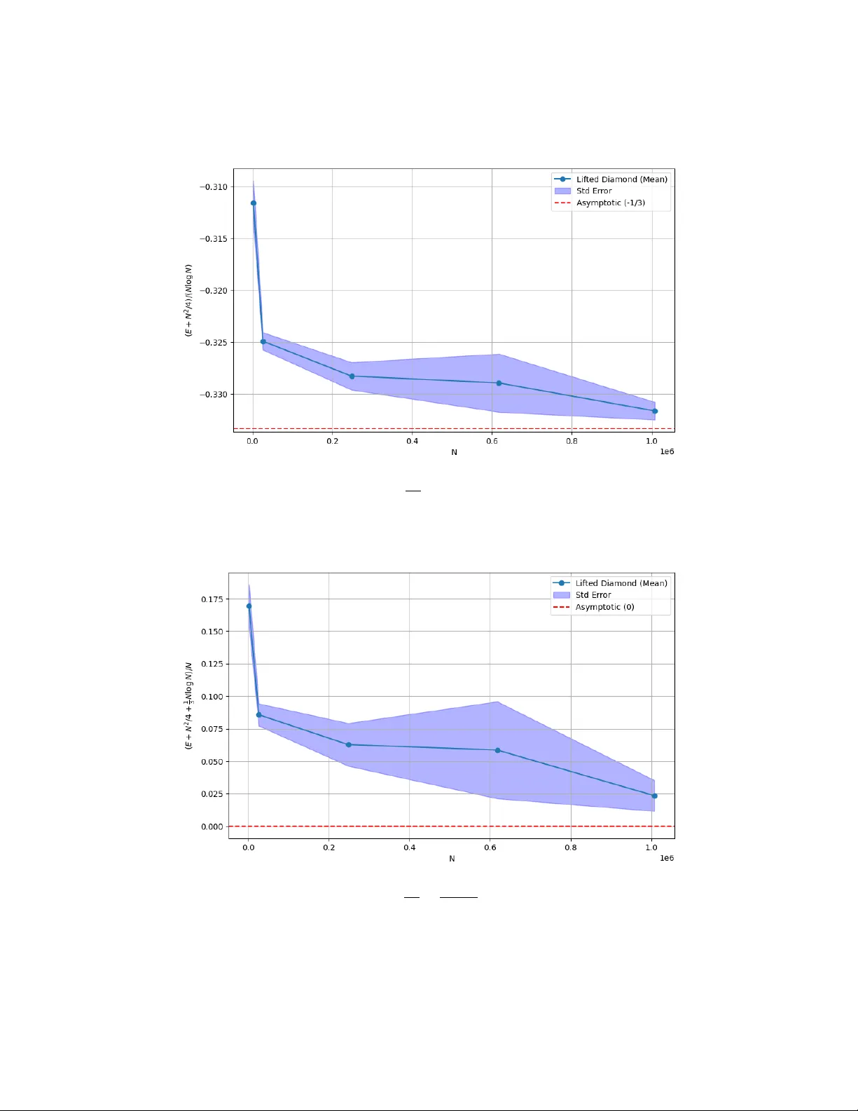
RANDOM POINTS ON S 3 WITH SMALL LOGARITHMIC ENER GY UJUÉ ET A YO AND P ABLO G. ARCE Abstract. W e analyse several constructions of random point sets on the sphere S 3 ⊂ R 4 ev aluating and comparing them through their discrete logarithmic energy: E 0 ( ω N ) = N X i,j =1 i  = j log 1 ∥ x i − x j ∥ , where ω N = { x 1 , . . . , x N } ⊂ S 3 . Using the Hopf fibration, w e lift a range of well-distributed families of p oints from the 2 -dimensional sphere - including uniformly random p oints, antipo dally symmetric sets, determinantal point processes, and the Diamond ensemble - to S 3 , in order to assess their energy performance. In particular, we carry out this asymptotic analysis for the Spherical ensem ble (a w ell kno wn determinantal point process on S 2 ), obtaining as a result a family of p oints on the 3 -dimensional sphere whose logarithmic energy is asymptotically the lowest achieved to date. This, in turn, provides a new upper b ound for the minimal logarithmic energy on S 3 . Although an analytic treatment of the lifted Diamond ensem ble remains elusive, extensive simulations presented here sho w that its empirical energies lie below all other deterministic and non-deterministic constructions considered. T ogether, these results sharp en the quantitativ e link b etw een p oten tial-theoretic optima on S 2 and S 3 and provide b oth theoretical and numerical benchmarks for future work. 1. Introduction and main resul ts 1.1. Logarithmic energy on S 2 . The problem of distributing p oin ts on a sphere so as to minimize a certain energy or maximize mutual distances is a classic topic in p otential theory and discrete geometry . One notable example is Whyte’s pr oblem , whic h asks for the arrangement of N p oin ts on the unit 2 -dimensional sphere, S 2 , that maximizes the pro duct of all pairwise distances. Equiv alen tly , this problem seeks to minimize the lo garithmic ener gy of N p oin ts on S 2 . F or a configuration Date : F ebruary 13, 2026. 2020 Mathematics Subje ct Classific ation. Primary 31C20; Secondary 52C35, 60G55, 82B21. K ey wor ds and phr ases. Logarithmic energy; Hopf fibration; determinantal p oin t processes; Diamond ensemble; Spherical ensemble; Harmonic ensemble. The authors hav e b een supp orted by gran t PID2020-113887GB-I00 funded by MCIN/AEI/10.13039/501100011033. The first author has also b een supp orted by the starting grant from FBBV A asso ciated with the prize José Luis R ubio de F rancia and by the Ramón y Cajal Programme of the Spanish Ministry of Science, Innov ation and Univ ersities, through the Agencia Estatal de Inv estigación (AEI), co-funded by the European Social F und Plus (ESF+), under grant R YC2024-049105-I. 1 2 UJUÉ ET A YO AND P ABLO G. AR CE ω N = { x 1 , . . . , x N } ⊂ S 2 , the discrete logarithmic energy is defined by E 0 ( ω N ) := N X i,j =1 i  = j log 1 ∥ x i − x j ∥ , where ∥ · ∥ denotes the Euclidean distance. Poin ts whic h minimize E 0 ( ω N ) are often called lo garithmic p oints or el liptic F ekete p oints . The problem of minimizing the logarithmic energy has special significance - for instance, it features in Smale’s sev enth problem on the asymptotic distribution of optimal configurations on the sphere, see [ 25 ]. P otential theory shows that the equilibrium measure for the logarithmic p oten tial on S d is the normalized surface area measure [ 8 ]. Accordingly , one exp ects that, as N → ∞ , configurations minimizing (or nearly minimizing) the logarithmic energy E 0 b ecome asymptotically uniformly distributed on the sphere. In the case of S 2 , this equidistribution has b een rigorously established, and the minimal logarithmic energy gro ws lik e N 2 , in agreemen t with the energy of a uniformly c harged spherical shell. Recen t work has further refined this picture b y deriving precise asymptotic expansions of the minimum energy; see [ 21 ] for a comprehensiv e account of the current state of the art. 1.2. Minimal logarithmic energy on S 3 . Compared to the 2 -dimensional sphere, m uch less is known ab out logarithmic energy minimization on the 3 -dimensional sphere S 3 = { ( x 1 , x 2 , x 3 , x 4 ) ∈ R 4 : x 2 1 + x 2 2 + x 2 3 + x 2 4 = 1 } . Finding and characterizing optimal discrete configurations on S 3 is a challenging problem. The higher dimensional geometry and the absence of a simple explicit parametrization for S 3 mak e the problem non-trivial. The current state of the art of the asymptotic expansion of the minimal logarithmic energy on S 3 is due to different authors [ 8 , 9 , 11 , 24 ] and is presented in the following equation. (1) min ω N ⊂ S 3 E 0 ( ω N ) = − N 2 4 − 1 3 N log N + O ( N ) , with ω N = { x 1 , . . . , x N } ⊂ S 3 . The b est upp er b ound for the minimal logarithmic energy kno wn to date is given in [ 7 ], where the authors in tro duce a random configuration of N p oin ts called the Harmonic ensem ble, denoted in the present w ork b y X N H . In [ 7 ], the authors compute the asymptotic expansion of the expected logarithmic energy of N p oin ts drawn from the Harmonic ensemble when N go es to infinit y , obtaining (2) E ω N ∼X N H [ E 0 ( ω N )] = − 1 4 N 2 − 1 3 N log N + C H N + o ( N ) , with C H = 1 3 log 1 3 + log 2 + ψ 0  3 2  + 1 3 ≈ 0 . 70 . . . where ψ 0 = ( log Γ) ′ is the digamma function. This expansion provides the sharp est kno wn upp er b ound for the minimal logarithmic energy . RANDOM POINTS ON S 3 WITH SMALL LOGARITHMIC ENERGY 3 1.3. Hopf fibration. In this work, we introduce and advocate for the use of the Hopf fibr ation in tac kling the S 3 problem. The Hopf fibration is a remarkable construction introduced b y H. Hopf in 1931 [ 14 ], which realizes the 3 -dimensional sphere as a non-trivial circle bundle ov er a 2 -dimensional base. A natural and intrinsic form ulation of the Hopf fibration is obtained b y viewing S 3 as the unit sphere in C 2 , S 3 = { ( z 1 , z 2 ) ∈ C 2 : | z 1 | 2 + | z 2 | 2 = 1 } , and by considering the free action of the circle group S 1 = { e iθ : θ ∈ [0 , 2 π ) } giv en b y e iθ · ( z 1 , z 2 ) = ( e iθ z 1 , e iθ z 2 ) . The orbits of this action are circles con tained in S 3 , and the corresp onding quotient space is the complex pro jective line, S 3 / S 1 ∼ = CP 1 . The asso ciated quotient map (3) π : S 3 − → CP 1 , ( z 1 , z 2 ) 7− → [ z 1 : z 2 ] , defines the Hopf fibration with base space CP 1 and fibre S 1 . The classical form ulation of the Hopf fibration takes S 2 as its base, whic h is reco vered b y identifying CP 1 with the Riemann sphere. Prop osition 1.1. Ther e exists a C 1 (in fact, smo oth) diffe omorphism Φ : S 2 − → CP 1 such that the push-forwar d of the spheric al surfac e me asur e on S 2 c oincides, up to a c onstant factor, with the F ubini-Study volume form on CP 1 . Mor e pr e cisely, if σ denotes the surfac e ar e a me asur e on S 2 and d v ol F S the F ubini–Study volume form on CP 1 normalize d by vol F S ( CP 1 ) = π , then d v ol F S = 1 4 Φ # σ. In p articular, the Jac obian determinant of Φ satisfies Jac(Φ) = 1 4 , Jac(Φ − 1 ) = 4 . Pr o of (sketch). Iden tify CP 1 with the Riemann sphere and consider the stereographic pro jection from the north p ole N = (0 , 0 , 1) ∈ S 2 , φ : S 2 \ { N } − → C , φ ( x, y , z ) = x + iy 1 − z . Extending by φ ( N ) = ∞ and comp osing with the standard affine chart C  → CP 1 yields a smo oth bijection Φ : S 2 − → CP 1 . Its inv erse is explicitly given, in affine co ordinates w ∈ C , by Φ − 1 ([1 : w ]) =  2 Re w 1 + | w | 2 , 2 Im w 1 + | w | 2 , | w | 2 − 1 1 + | w | 2  , whic h shows that Φ is a C 1 diffeomorphism (in fact, C ∞ ). 4 UJUÉ ET A YO AND P ABLO G. AR CE In stereographic co ordinates, the spherical surface measure and the F ubini-Study v olume form are given b y dσ = 4 (1 + | w | 2 ) 2 dA ( w ) , d v ol F S = 1 (1 + | w | 2 ) 2 dA ( w ) , where dA denotes the Leb esgue measure on C . Comparing these expressions yields d v ol F S = 1 4 dσ, whic h implies the stated v alues of the Jacobian determinants. This expression is consisten t with the earlier identit y d v ol FS = 1 4 Φ # σ , as we are here working in lo cal co ordinates on C ⊂ CP 1 , where the pushforw ard Φ # σ coincides with the standard surface area measure dσ on the Riemann sphere. □ Comp osing the pro jection π with the diffeomorphism Φ − 1 : CP 1 − → S 2 in tro duced in Theorem 1.1 , one obtains the map h = Φ − 1 ◦ π : S 3 − → S 2 , whic h admits the explicit real-co ordinate expression h ( a, b, c, d ) = ( a 2 + b 2 − c 2 − d 2 , 2( ad + bc ) , 2( bd − ac )) , for ( a, b, c, d ) ∈ S 3 ⊂ R 4 . It is easy to chec k that the image of h lies on S 2 , since the sum of the squares of its comp onen ts equals ( a 2 + b 2 + c 2 + d 2 ) 2 = 1 . F or eac h p oint P ∈ S 2 , the preimage h − 1 ( P ) is a great circle in S 3 , called the fibre ov er P . Thus, S 3 is decomp osed into disjoin t circles, one ab o ve eac h p oint of the base space. An explicit parametrization of the fibre ov er a p oin t ( p 1 , p 2 , p 3 ) ∈ S 2 is given by (4) h − 1 ( p 1 , p 2 , p 3 ) =  (1 + p 1 ) cos t, (1 + p 1 ) sin t, p 2 sin t − p 3 cos t, p 2 cos t + p 3 sin t  p 2(1 + p 1 ) , with t ∈ [0 , 2 π ) . This viewp oint shows that the Hopf fibration ma y b e equiv alen tly regarded as a fibration ov er S 2 or ov er CP 1 , the tw o base spaces b eing related by the diffeomorphism Φ . In the present work, this dual interpretation will play a key role in transferring p oin t pro cesses and geometric structures b et w een S 3 , S 2 , and CP 1 . 1.4. Main results. 1.4.1. Fibr e d c onstructions. Via the Hopf fibration, well-distributed configurations on S 2 can b e lifted to S 3 , yielding a direct link b et w een p oint sets on the tw o spheres. F or example, supp ose that w e start with a configuration of r "base" p oints on S 2 that are reasonably uniformly distributed. Ab o v e each suc h base p oint y j ∈ S 2 , consider its fibre h − 1 ( y j ) ∼ = S 1 in S 3 . W e can place k p oin ts along eac h of these fibres (for instance, k equally spaced p oin ts on the circle). This construction pro duces a set of N = r k p oin ts on S 3 . If the r base p oin ts on S 2 are well-spaced and the k fibre p oin ts on each circle are evenly spaced, then one exp ects that the resulting N -p oin t configuration on S 3 inherits a go od separation and distribution. Recen t RANDOM POINTS ON S 3 WITH SMALL LOGARITHMIC ENERGY 5 results supp ort this approac h; see, for instance, [ 4 ], where the Hopf fibration is generalized to higher-dimensional spheres and exploited as a to ol for constructing w ell-distributed p oin t sets. A similar strategy is adopted by Beltrán, Carrasco, F erizović and Lóp ez-Gómez [ 3 ] to distribute p oints in S O (3) . In the rest of this article, we develop the theoretical framework for this lifting tec hnique and analyse the logarithmic energy of the resulting configurations. W e work with p oints sampled uniformly from S 2 , together with their antipo dal counterparts. F or these p oin t configurations, we obtain the asymptotic E [ E 0 ( ω N )] = − 1 4 N 2 + C N , where ω N = { x 1 , . . . , x N } ⊂ S 3 , with C a constant dep ending on the family of p oin ts. One can chec k that the first term of the asymptotic expansion is correct, but the second term is already of the wrong order (see equation ( 1 )). A comparison of the linear-term constant C for the differen t families of uniform p oints is giv en in T able 1 . Distribution Constan t on the linear term Uniform S 3 1 / 4 Uniform S 3 and symmetry 1 2 − log 2 = − 0 . 193 ... Uniform S 2 and fibres 1 − 2 log 2 = − 0 . 386 ... Uniform S 2 , symmetry and fibres 7 2 (1 − log 2) − log 7 = − 0 . 871 ... T able 1. Linear-term co efficients for different uniform distributions. W e also study other types of random pro cess, known as determinantal p oin t pro cesses. In particular, we consider the Harmonic ensemble on the 2 -dimensional sphere in troduced in [ 7 ], and the Spherical ensem ble introduced in [ 16 ]. F or the latter, we obtain the main theorem of the pap er. Finally , w e study p oin t sets coming from the Diamond ensemble, as defined in [ 5 ]. 1.4.2. Notation. W e refer to a sequence of sets of p oints { ω r } r ∈ N where each ω r = { x 1 , . . . , x r } is a set of r p oin ts on the corresp onding sphere as a family of p oints . In particular, we w ork with the following families: • U r S 2 is a set of r uniformly distributed p oin ts on S 2 . • ¯ U r S 2 is a set consisting of r / 2 uniformly distributed p oints on S 2 and their r / 2 antipo dal counterparts. • X r H is a set of r p oin ts on S 2 follo wing the distribution of the Harmonic ensem ble. • X r S is a set of r p oin ts on S 2 follo wing the distribution of the Spherical ensem ble. • ⋄ ( r ) is a set of r p oin ts on S 2 follo wing the distribution of the Diamond ensem ble. W e use the symbol ↑ k H ( ω r ) to denote the set of N = k r p oin ts obtained by the pro cedure of considering k ro ots of unity on the fibre corresp onding to each p oint in ω r . F or example, if we fibre r p oin ts coming from the Spherical ensemble in S 2 and take k points in each fibre, we denote it by ↑ k H ( X r S ) . 6 UJUÉ ET A YO AND P ABLO G. AR CE 1.4.3. A new b ound for the minimal lo garithmic ener gy on S 3 . The Spheric al ensem- ble is a determinan tal p oint pro cess on the Riemann sphere that arises in random matrix theory . It was first obtained by stereographically pro jecting the generalized eigen v alues of tw o indep endent Ginibre matrices onto the sphere [ 17 ]. This construc- tion yields a rotationally in v ariant distribution of N p oin ts on S 2 . In particular, the Spherical ensemble has a joint density prop ortional to the pro duct of squared pairwise distances (a spherical V andermonde determinant), which is the hallmark of determinan tal p oint pro cesses and leads to strong mutual repulsion b etw een p oin ts. Consequen tly , the p oints tend to spread out uniformly on the sphere. Despite b eing random, this ensemble exhibits nearly optimal uniformity in the sense of p oten tial theory: it achiev es v ery low discrepancy and near-minimal Riesz energy , on par with (and in some cases outp erforming) the b est deterministic p oint configurations [ 1 , 11 , 18 ]. In this pap er, we prov e that the exp ected logarithmic energy of p oin ts coming from the fibred Spherical ensem ble pro vides the b est upp er b ound for the minimal logarithmic energy on S 3 . Theorem 1.2. L et A B b e a r ational appr oximation of 3 2 π 4 3 ≈ 0 . 44 . . . . L et ↑ k H ( X r S ) b e a set of N = k r p oints obtaine d by taking k p oints e qual ly sp ac e d, r andomly r otate d in e ach fibr e S 1 of S 3 , with r esp e ct to r = A B k 2 p oints dr awn fr om the Spheric al ensemble X r S in S 2 . Then, E ω N ∼↑ k H ( X r S ) [ E 0 ( ω N )] = − N 2 4 − 1 3 N log N + N √ π 4  B A  1 / 2 − log  B A  1 / 3 !! + o ( N ) . In p articular, the c o efficient of the line ar term tends to 1 3  2 + log 9 π 64  as A B mor e closely appr oximates 3 2 π 4 3 . R emark 1.3 . Note that for a given n um b er of p oints k w e ha ve to find a suitable appro ximation A B that makes r an in teger num b er. This leads us to the following upp er b ound for the minimal logarithmic energy on S 3 . Corollary 1.4. F or an infinite se quenc e of p ositive inte ger numb ers { n i } i ∈ N , the fol lowing upp er b ound holds: min ω n i ⊂ S 3 E 0 ( ω n i ) ≤ − N 2 4 − 1 3 N log N + C S N + o ( N ) , with C S = 1 3  2 + log 9 π 64  . W e recall that, to date, the b est result is the one obtained by the authors in [ 7 ], presen ted in equation ( 2 ). The asymptotic expansions given by b oth families match up to the linear term, as b oth correctly repro duce the terms in N 2 and N log N seen in equation ( 1 ). Comparing the co efficients of the linear terms in b oth expansions, w e hav e: C S = 1 3  2 + log 9 π 64  = 0 . 39 ... < C H = 1 3 log 1 3 + log 2 + ψ 0  3 2  + 1 3 = 0 . 70 ... RANDOM POINTS ON S 3 WITH SMALL LOGARITHMIC ENERGY 7 This allo ws us to conclude that the Spherical ensemble, in conjunction with the Hopf fibration, provides a p oin t pro cess on S 3 , ↑ k H ( X r S ) , with asymptotically low er logarithmic energy than the Harmonic ensemble, resulting in the configuration of p oin ts with the lo west logarithmic energy prov ed to date. 1.4.4. The lifte d Harmonic ensemble. The Harmonic ensemble pro vides a natural and well-studied determinan tal p oint pro cess on S 2 , and its inv ariance prop erties mak e it a conv enien t b enchmark for energy comparisons after lifting via the Hopf fibration. The p oint configurations obtained in this wa y repro duce b oth the leading and second-order terms in the asymptotic expansion of the logarithmic energy . Ho wev er, as shown in Theorem 3.9 , the third-order term deviates from the exp ected b eha viour: instead of b eing linear, it exhibits an additional log log N factor. This deviation indicates a limitation of the lifting procedure when applied to the Harmonic ensem ble, particularly in capturing the finer asymptotic structure. 1.4.5. The lifte d Diamond ensemble. Among the different families of N p oin ts that ha ve b een prop osed on the 2 -dimensional sphere, the Diamond ensemble introduced b y Beltrán and Etay o [ 5 ] and then refined in [ 6 ] presently attains the low est known logarithmic energy . The theoretical low er b ound for the minimal logarithmic energy of N p oints on S 2 b eha v es asymptotically as (5)  1 2 − log 2  N 2 − 1 2 N log N + C N , C = − 0 . 0568456 . . . , see [ 21 ]. Configurations drawn from the Diamond ensemble are N × 0 . 0076 . . . far aw a y from this rate and thereby outperform all other deterministic and random constructions curren tly av ailable. A configuration with N p oin ts is built as follo ws. First, select K parallels of latitude z k and allocate to the k th parallel r k p oin ts suc h that P K k =1 r k = N − 2 . The r k p oin ts on the k th parallel are placed at equal angular separations in longitude, and the en tire parallel is then rotated by a random phase c hosen uniformly in [0 , 2 π ) . Finally , the North and South p oles are app ended, yielding a total of N p oints. Motiv ated b y its success on S 2 , w e attempted to transplan t the Diamond ensem ble to the 3 -dimensional sphere via the Hopf fibration. Despite the effort, the fibre-lifting tec hnique did not lead to tractable analytic expressions for the resulting logarithmic energy , as sho wn in Section A.1 . W e therefore rep ort here solely on the numerical evidence, which nev ertheless offers meaningful insight into the p erformance of the lifted Diamond configurations on S 3 . This has b een carried out using [ 22 ] from Python. The Numba library [ 19 ] has also b een employ ed to accelerate computations b y translating part of the co de to C. When transitioning to the sphere S 3 using the Hopf fibration, one parameter whose optimal v alue is unknown is the num ber of p oints p er fibre, denoted as k . V arious options hav e b een experimented with for c ho osing k , and it has been found to b e optimal to take k = p α , where p is the n um ber of parallels (a v alue that determines the other parameters of the Diamond ensemble). Multiple simulations ha ve b een conducted for differen t v alues of α , with the optimal v alue being approximately α ≈ 1 . 2 . As sho wn in Figures 1 and 2 , for α = 1 . 2 the co efficien t of the N log N term in the asymptotic expansion of the energy tends to − 1 / 3 , in agreement with equation ( 1 ), while the co efficient of the linear term appears to approac h 0 , which compares fa vourably with the other constructions considered in this work. 8 UJUÉ ET A YO AND P ABLO G. AR CE Figure 1.  E ω N ∼↑ k H ( ⋄ r ) [ E 0 ( ω N )] + N 2 4  / N log N plotted against the n umber of p oin ts, where E ω N ∼↑ k H ( ⋄ r ) [ E 0 ( ω N )] represen ts the exp ected v alue of the logarithmic energy of the lifted configuration of p oints coming from the Diamond ensemble through the Hopf fibration. A veraged o ver 5 runs with differen t random seeds. Figure 2.  E ω N ∼↑ k H ( ⋄ r ) [ E 0 ( ω N )] + N 2 4 + N log N 3  / N plotted against the num b er of points, where E ω N ∼↑ k H ( ⋄ r ) [ E 0 ( ω N )] represen ts the expected v alue of the lifted configuration of points coming from the Diamond ensemble through the Hopf fibration. A veraged o ver 5 runs with different random seeds. RANDOM POINTS ON S 3 WITH SMALL LOGARITHMIC ENERGY 9 1.4.6. Or ganization of the p ap er. Section 1: In troduction and main results: W e state the logarithmic energy problem on S 3 , introduce the Hopf fibration lifting strategy , and summarize the principal analytic and numerical findings. Section 2: Uniformly distributed points: W e analyse energies for configura- tions of p oints obtained from uniform distributions on S 3 and from uniform p oin ts on S 2 lifted by Hopf fibres. Section 3: Determinan tal P oin t Processes: W e develop the p oten tial-theoretic framew ork for determinan tal p oin t pro cesses (Spherical ensemble, Harmonic ensem ble, etc.) and derive their energy expansions after lifting. Section 4: Proof of the main results: W e collect auxiliary lemmas and give full pro ofs of the asymptotic b ounds, including the new upper b ound for the minimal logarithmic energy on S 3 . App endix A: The Diamond ensem ble: W e recall the construction of the Dia- mond ensem ble on S 2 , detail its fibre lifting to S 3 , and rep ort n umerical results. 2. Uniforml y distributed points W e can sample i.i.d. uniformly distributed p oints in S 3 b y taking ( x, y , z , t ) ⊂ R 4 suc h that (6)          x = √ 1 − v 2 √ 1 − u 2 cos φ y = √ 1 − v 2 √ 1 − u 2 sin φ z = √ 1 − v 2 u t = v with      φ ∈ [0 , 2 π ] uniform , u ∈ [ − 1 , 1] uniform , v ∈ [ − 1 , 1] with density f V ( v ) , where f V ( v ) = 2 π p 1 − v 2 . Lemma 2.1. L et ω N = { p 1 , . . . , p N } b e a set of N i.i.d. uniformly distribute d p oints in S 3 , then: E ϕ i ,u i ,v i , 1 ≤ i ≤ N [ E 0 ( ω N )] = − 1 4 N 2 + 1 4 N , wher e p i = ( x i , y i , z i , t i ) ar e as in e quation ( 6 ) . Pr o of. Using the notation from equation ( 6 ), the distance b etw een t wo random i.i.d. uniformly distributed p oints is || p i − p j || =  2 − 2 q 1 − v 2 i q 1 − v 2 j  q 1 − u 2 i q 1 − u 2 j cos( φ i − φ j ) + u i u j  − 2 v i v j  1 / 2 . S 3 is a 2-p oint homogeneous space, that is, for every p 1 , p 2 , q 1 , q 2 ∈ S 3 suc h that ∥ p 1 − p 2 ∥ = ∥ q 1 − q 2 ∥ there exists an isometry of S 3 , that we denote by i , such that i ( p 1 ) = q 1 and i ( p 2 ) = q 2 . Hence w e can simplify the computations of the exp ected v alue of the distance by taking p i = (0 , 0 , 0 , 1) . Then, for a fixed j , (7) E ϕ j ,u j ,v j [ − log || (0 , 0 , 0 , 1) − p j || ] = − Z 1 − 1 2 π q 1 − v 2 j log( p 2 − 2 v j ) dv j 10 UJUÉ ET A YO AND P ABLO G. AR CE = − 1 π Z π 0 sin 2 θ ln (2 − 2 cos θ ) dθ = − ln (2) − 2 π Z π 0 sin 2 θ ln  sin θ 2  dθ , after the appropriate change of v ariables v j = cos θ . F or the integral, taking ϕ = θ 2 and using that sin(2 ϕ ) = 2 sin ϕ cos ϕ , we hav e − 2 π Z π 0 sin 2 θ ln  sin θ 2  dθ = − 2 π Z π / 2 0 4 sin 2 ϕ cos 2 ϕ ln (sin ϕ ) 2 dϕ. The last integral resem bles an incomplete b eta function I ( a, b ) = Z π / 2 0 sin 2 a ϕ cos 2 b ϕdϕ = 1 2 B  a + 1 2 , b + 1 2  . If we differentiate the last expression with resp ect to a , we obtain ∂ I ∂ a ( a, b ) = Z π / 2 0 2 ln(sin ϕ ) sin 2 a ϕ cos 2 b ϕdϕ = 1 2 B  a + 1 2 , b + 1 2   ψ  a + 1 2  + ψ ( a + b + 1)  . It only remains to ev aluate the last expression at a = 1 and b = 1 : ∂ I ∂ a (1 , 1) = π (1 − 4 ln 2) 32 . W e conclude with E ϕ j ,u j ,v j [ − log || (0 , 0 , 0 , 1) − p j || ] = − 1 4 . The exp ected v alue of the logarithmic energy for N points will then b e E ϕ i ,u i ,v i , 1 ≤ i ≤ N [ E 0 ( ω N )] = − 1 4 N ( N − 1) = − 1 4 N 2 + 1 4 N , where ω N = { p 1 , . . . , p N } and p i = ( x i , y i , z i , t i ) are as in equation ( 6 ). □ W e reason as follows: given a single p oint on the sphere, the p oint and the an tip o dal p oin t (obtained through cen tral symmetry on the sphere) form the b est p ossible distribution of tw o p oin ts. F urthermore, for the energy calculation with a third p oint, eac h of the p oin ts can b e treated as randomly and uniformly distributed p oin ts. Therefore, this suggests that generating N / 2 points and then applying central symmetry should provide b etter-distributed p oints. Lemma 2.2. Consider M i.i.d. uniformly distribute d p oints on S 3 , and let ω N denote the set of N = 2 M p oints c onsisting of these M p oints to gether with their antip o dal p oints. Then: E ϕ i ,u i ,v i , 1 ≤ i ≤ M [ E 0 ( ω N )] = − 1 4 N 2 +  1 2 − log 2  N , wher e ω N = { p 1 , . . . , p N } and p i = ( x i , y i , z i , t i ) ar e as in e quation ( 6 ) and p M + i is the antip o dal p oint of p i for 1 ≤ i ≤ M . Pr o of. W e tak e M = N / 2 i.i.d. uniformly distributed points in S 3 . Then, the asymptotic expansion of the logarithmic energy consists on the sum of tw o terms: (1) The energy con tributed by antipo dal p oints. RANDOM POINTS ON S 3 WITH SMALL LOGARITHMIC ENERGY 11 (2) The energy con tributed by non-antipo dal p oints. Fixing a p oint p i , we hav e from equation ( 7 ) that E ϕ i ,u i ,v i ,ϕ j ,u j ,v j [ − log || p i − p j || ] = − 1 4 , for p j dra wn uniformly at random from S 3 . F urthermore, for the antipo dal p oin t, w e hav e: E ϕ i ,u i ,v i [ − log || p i − ( − p i ) || ] = − log || 2 p i || = − log 2 . T aking b oth terms into account, the asymptotic expansion of the logarithmic energy is E ϕ i ,u i ,v i , 1 ≤ i ≤ M [ E 0 ( ω N )] = − 1 4 N ( N − 2) − N log 2 = − 1 4 N 2 +  1 2 − log 2  N . □ One can verify that this energy is lo w er than that of the fully uniform distribution on S 3 (cf. Theorem 2.1 ). 2.1. Uniform distribution on S 2 and the use of Hopf fibration. Now we use the uniform distribution in S 2 , whose p oints can b e written as: ( x, y , z ) ∈ R 3 :      x = √ 1 − u 2 cos φ y = √ 1 − u 2 sin φ z = u with ( φ ∈ [0 , 2 π ] uniformly , u ∈ [ − 1 , 1] uniformly . Prop osition 2.3. L et ν M b e a set of M i.i.d. uniformly distribute d p oints in S 2 . F or e ach p oint in ν M let us c onsider a set of k r o ots of unity on the fibr e c orr esp onding to the inverse of the p oint via the Hopf fibr ation. L et ω N b e set of al l N = k M p oints obtaine d on S 3 by this pr o c e dur e that we denote by ↑ k H ( U M S 2 ) . Then: E ω N ∼↑ k H ( U M S 2 ) [ E 0 ( ω N )] = − 1 4 N 2 + (1 − 2 log 2) N . Pr o of. See Section 4.2 . □ A symmetry argument similar to the one used with the uniform distribution on S 3 can b e deduced here. T wo possibilities arise in this case. On one hand, central symmetry in S 3 with p oints on the Hopf fibres could b e used. How ev er, since the fibres are great circles, central symmetry would place more p oin ts on the same fibre, which would go against the optimal choice of the num b er of p oints p er fibre. Therefore, we chose to use symmetry in S 2 to hav e b etter-distributed p oin ts on S 2 and calculate the fibres afterwards. Prop osition 2.4. Consider M / 2 ∈ N i.i.d. uniformly distribute d p oints on S 2 , and let ν M denote the set of M p oints c onsisting of these M / 2 p oints to get her with their antip o dal p oints. F or e ach p oint in ν M let us c onsider a set of k r o ots of unity on the fibr e c orr esp onding to the inverse of the p oint via the Hopf fibr ation. L et ω N b e set of al l N = k M p oints obtaine d on S 3 by this pr o c e dur e that we denote by ↑ k H ( ¯ U M S 2 ) . Then: E ω N ∼↑ k H ( ¯ U M S 2 ) [ E 0 ( ω N )] = − 1 4 N 2 +  7 2 (1 − log 2) − log 7  N . Pr o of. The computation of this asymptotic expansion of the energy is shown in Section 4.2 . □ 12 UJUÉ ET A YO AND P ABLO G. AR CE Comparing linear terms, one sees that the best results among the different uniform distributions are obtained by taking the uniform distribution on S 2 , applying cen tral symmetry , and then lifting to S 3 via the Hopf fibration. How ev er, none of the p oint configurations presented here ac hiev es the optimal gro wth order in the N log ( N ) term (the second order term), whereas those presented in the next section do. T able 1 compares the co efficients of the linear term for each uniform distribution. 3. Determinant al point pr ocesses In this section, w e presen t the basic theoretical foundations of determinan tal p oin t pro cesses in order to enable the computation of the asymptotic expansion of the exp ected v alue of their logarithmic energy . A comprehensive developmen t is b ey ond the scop e of this work and can b e found in [ 15 ]. W e recall that a Polish space is a separable, completely metrizable top ological space. Let Λ b e a lo cally compact, Polish space endow ed with a Radon measure µ . A simple pro cess of N p oin ts in Λ is a random v ariable in Λ N (or equiv alen tly , N random v ariables simultaneously chosen in Λ ). Some point pro cesses admit associated in tensity functions, defined as follows. Definition 3.1. Let Λ and X b e a space and a simple p oin t pro cess of N p oin ts as defined previously . Intensit y functions are functions, if any exist, ρ k : Λ k → [0 , ∞ ) , 1 ≤ k ≤ N suc h that for any family of pairwise disjoint subsets D 1 , ..., D k of Λ , the following holds: E x ∼X " k Y i =1  ( x ∩ D i ) # = Z Q D i ρ k ( x 1 , ..., x k ) dµ ( x 1 , ..., x k ) . In addition, we shall require that ρ k ( x 1 , . . . , x k ) v anish if x i = x j for some i  = j . Prop osition 3.2. L et Λ and X b e a sp ac e and a simple p oint pr o c ess of N p oints with asso ciate d intensity functions ρ k , 1 ≤ k ≤ N , as in the pr evious definition. F or any me asur able function f : Λ k → [0 , ∞ ) , k ≥ 1 , the fol lowing holds: E x ∼X   X i 1 ,...,i k distinct f ( x i 1 , ..., x i k )   = Z y 1 ,...,y k ∈ Λ f ( y 1 , ..., y k ) ρ k ( y 1 , ..., y k ) dµ ( y 1 , ..., y k ) . Pr o of. W e refer to [ 12 , Equation 1.13]. □ Some simple p oin t pro cesses with asso ciated in tensity functions ρ k , 1 ≤ k ≤ N , ha ve in tensit y functions of the form (8) ρ k ( x 1 , ..., x k ) = det ( K ( x i , x j ) 1 ≤ i,j ≤ k ) for K : Λ × Λ − → C a measurable function. Such pro cesses are called determinantal p oint pr o c ess ( dpp ). The existence of determinantal p oint pro cesses under suitable assumptions, and with prescrib ed structural properties, is guaranteed by the Macchi– Soshnik ov theorem, which w e no w recall. RANDOM POINTS ON S 3 WITH SMALL LOGARITHMIC ENERGY 13 Theorem 3.3 (Macchi–Soshnik o v) . L et Λ b e as describ e d ab ove and let H ⊂ L 2 (Λ) b e a subsp ac e of dimension N . Then ther e exists a p oint pr o c ess X H on Λ c onsisting of N p oints, whose k -p oint intensity functions ar e given by ρ k ( x 1 , ..., x k ) = det ( K H ( x i , x j ) 1 ≤ i,j ≤ k ) wher e K H denotes the r epr o ducing kernel of H and we say that X H is a determinantal p oint pr o c ess with kernel K H . Pr o of. Pro ofs of this theorem can b e found in [ 20 , 26 ], and in a formulation closer to the present one in [ 15 , Theorem 4.5.5]. □ Corollary 3.4. Under the assumptions of The or em 3.3 , the exp e cte d numb er of p oints satisfies N = E X ∼X H [ N ] = Z Λ K H ( p, p ) dµ ( p ) . In p articular, if the diagonal of the kernel K H ( p, p ) is c onstant (indep endent of p ), then ne c essarily K H ( p, p ) = N V ol(Λ) , and we say that K H is homo gene ous. Pr o of. W e take ϕ ≡ 1 and substitute it into the previous identit y . □ Corollary 3.5. Under the assumptions of The or em 3.3 , for any me asur able function f : Λ × Λ → [0 , 1) , one has E X ∼X H   X i  = j f ( x i , x j )   = Z Λ × Λ  K H ( p, p ) K H ( q , q ) −| K H ( p, q ) | 2  f ( p, q ) dµ ( p ) dµ ( q ) . Pr o of. It is a direct consequence of Theorem 3.2 and the definition of dpp . □ 3.1. Determinan tal p oin t processes on CP 1 and the Hopf fibration. Prop osition 3.6. L et ν r = { x 1 , . . . , x r } ⊂ CP 1 b e a set of r andom p oints fol lowing the distribution of a dpp that we denote by X r . F or e ach p oint in ν r let us c onsider a set of k r o ots of unity on the fibr e c orr esp onding to the inverse of the p oint via the Hopf fibr ation. L et ω N b e set of al l N = k r p oints obtaine d on S 3 by this pr o c e dur e that we denote by ↑ k H ( X r ) . Then: E ω N ∼↑ k H ( X r ) [ E 0 ( ω N )] = − r k log k − k 2 2 Z CP 1 × CP 1 log  1 + p 1 − < p , q > 2   K ( p , p ) 2 − | K ( p , q ) | 2  d p d q , wher e K is the kernel asso ciate d to X r . Pr o of. Let x 1 , ..., x r ∈ CP 1 b e obtained through a dpp with kernel K . W e choose, for eac h x i , an affine represen tativ e of unit norm, which we denote by the same sym b ol. Let i = √ − 1 denote the imaginary unit. Consider y ij = x i e i ( θ i + 2 πj k ) ∈ S 3 ⊆ C 2 , 1 ≤ i ≤ r , 1 ≤ j ≤ k , with θ i a random phase pic ked uniformly on [0 , 2 π ] , as the p oin ts in the fibres given b y the inv erse of the Hopf fibration in its complex form, see equation ( 3 ). In the computation of the expected logarithmic energy , t w o quantities are in v olv ed: 14 UJUÉ ET A YO AND P ABLO G. AR CE (1) The energy contributed b y pairs of p oints in the same fibre, summed ov er all the fibres (denote this quantit y by J 1 ). (2) The energy contributed by pairs of p oints in different fibres, (denote this quan tity b y J 2 ). Computation of J 1 . All the fibres are great circles with k p oin ts. Therefore, the quantit y J 1 equals the energy of one fibre multiplied by the num b er of fibres. F urthermore, it is imp ortan t to note that the distances do not dep end on θ i since all the p oints are on the same fibre. J 1 = r X i =1 1 2 π Z 2 π 0 E θ i     k − 1 X j 1 ,j 2 =0 j 1  = j 2 − log       e i ( θ i + 2 πj 1 k ) x i − e i ( θ i + 2 πj 2 k ) x i           dθ i = − r k − 1 X j 1 ,j 2 =0 j 1  = j 2 log    e i 2 πj 1 k − e i 2 πj 2 k    = − r k log k , where we hav e used the fact that || x i || = 1 and Theorem 4.1 . Computation of J 2 . J 2 = 1 4 π 2 E ν r ∼X r  P k − 1 j 1 ,j 2 =0 P r i 1 ,i 2 =1 i 1  = i 2 R 2 π 0 R 2 π 0 − log       e i ( θ i 1 + 2 πj 1 k ) x i 1 − e i ( θ i 2 + 2 πj 2 k ) x i 2       dθ i 1 dθ i 2  = E ν r ∼X r     k − 1 X j 1 ,j 2 =0 r X i 1 ,i 2 =1 i 1  = i 2 1 2 π Z π 0 − log(2 − 2 < x i 1 , x i 2 > cos θ ) dθ     = − k 2 2 E ν r ∼X r     r X i 1 ,i 2 =1 i 1  = i 2 log  1 + p 1 − < x i 1 , x i 2 > 2      , where the last integral was computed using Theorem 4.2 . W e conclude with Theo- rem 3.5 : J 2 = − k 2 2 E ν r ∼X r     r X i 1 ,i 2 =1 i 1  = i 2 log  1 + p 1 − < x i 1 , x i 2 > 2      = − k 2 2 Z CP 1 × CP 1 log  1 + p 1 − < p , q > 2   K ( p , p ) 2 − | K ( p , q ) | 2  d p d q . □ 3.2. The Spherical ensemble. A natural interpretation of the Spherical ensemble arises from the generalized eigenv alue problem asso ciated with a matrix p encil ( A, B ) , viewed in the complex pro jective space. More precisely , one considers the p oin ts ( α : β ) ∈ CP 1 suc h that det( αB − β A ) = 0 , RANDOM POINTS ON S 3 WITH SMALL LOGARITHMIC ENERGY 15 and identifies CP 1 with the Riemann sphere. It was sho wn by Krishnapur [ 16 ] that this construction defines a determinantal p oin t pro cess on CP 1 . The asso ciated correlation kernel can b e describ ed explicitly as follows. W riting x = [ p ] , y = [ q ] with p , q ∈ C 2 \ { 0 } , and with resp ect to the F ubini–Study volume normalized so that V ol( CP 1 ) = π , its correlation kernel is given b y   K CP 1 r ( x, y )   = r π      p ∥ p ∥ , q ∥ q ∥      r − 1 , p , q ∈ C 2 \ { 0 } . In particular, K CP 1 r ( x, x ) = r π . Via the diffeomorphism mapping the Riemann sphere onto the unit sphere S 2 (see Theorem 1.1 ), and using that the surface area measure on S 2 satisfies σ ( S 2 ) = 4 π , this construction induces a determinan tal p oin t process on S 2 whose correlation k ernel is given by   K S 2 r ( x, y )   = r 4 π  1 + ⟨ x, y ⟩ 2  r − 1 , x, y ∈ S 2 , where ⟨ x, y ⟩ denotes the Euclidean inner pro duct in R 3 . In particular, K S 2 r ( x, x ) = r 4 π . The prop erties of the Spherical ensem ble on S 2 are studied in depth b y Alishahi and Zamani [ 1 ], who, in particular compute the exp ected logarithmic energy of its p oin ts. The kernels K CP 1 r and K S 2 r are related by push-forw ard under the diffeomorphism iden tifying CP 1 with S 2 , together with the corresp onding Jacobian factor b etw een the F ubini–Study volume and the spherical surface measure. Prop osition 3.7. L et ν r b e a set of r r andom p oints sample d fr om the Spheric al ensemble X r S . F or e ach p oint in ν r let us c onsider a set of k r o ots of unity on the fibr e c orr esp onding to the inverse of the p oint via the Hopf fibr ation. L et ω N b e the set of al l N = k r p oints obtaine d on S 3 by this pr o c e dur e that we denote by ↑ k H ( X r S ) . Then, the asymptotic exp ansion of the lo garithmic ener gy of this family of p oints as N go es to infinity is E ω N ∼↑ k H ( X r S ) [ E 0 ( ω N )] = − N 2 4 − N log k + √ π 4 √ N k 3 / 2 − k 2 4 + k 2 O r k N ! . Pr o of. See Section 4.4.1 . □ An appropriate choice of k in terms of the num ber of p oints N leads to the asymptotic expansion presented in Theorem 1.2 : − N 2 4 − 1 3 N log N + N 3  2 + log 9 π 64  − 4 3 4 / 3 π 2 / 3 N 2 / 3 + O ( N 1 / 3 ) . Ho wev er, this expansion represen ts an impossible construction, as it holds for v alues of k that are not necessarily p ositive integers. In an y case, as explained in Section 4.4.2 , the constan t 1 3  2 + log 9 π 64  can b e appro ximated with arbitrary precision (although this imp oses restrictions on the num ber of p oin ts). 16 UJUÉ ET A YO AND P ABLO G. AR CE 3.3. The Harmonic ensemble. Let Y ℓm : S 2 → C b e the standard spherical harmonics of degree  ≥ 0 and order m ∈ {− , . . . ,  } , orthonormal with resp ect to the normalized surface measure on S 2 , normalized by σ ( S 2 ) = 4 π . F or a given in teger L ≥ 0 , let H ≤ L ⊂ L 2 ( S 2 ) denote the ( L + 1) 2 -dimensional subspace spanned b y all spherical harmonics of degree  ≤ L . The Harmonic ensemble on S 2 is defined as the determinantal p oin t pro cess whose correlation kernel K L ( x, y ) is the integral kernel of the orthogonal pro jection on to H ≤ L . Equiv alen tly , if { Y ℓm : 0 ≤  ≤ L, −  ≤ m ≤  } is an orthonormal basis of H ≤ L , then K S 2 L ( x, y ) = L X ℓ =0 ℓ X m = − ℓ Y ℓm ( x ) Y ℓm ( y ) , x, y ∈ S 2 . With resp ect to the surface area measure σ on S 2 one has K S 2 L ( x, x ) = dim( H ≤ L ) 4 π = ( L + 1) 2 4 π . By the addition theorem for spherical harmonics, the k ernel admits a rotationally in v ariant expression dep ending only on the Euclidean inner pro duct ⟨ x, y ⟩ : K S 2 L ( x, y ) = 1 4 π L X ℓ =0 (2  + 1) P ℓ ( ⟨ x, y ⟩ ) = L + 1 4 π P (1 , 0) L  ⟨ x, y ⟩  , where P ℓ denotes the Legendre p olynomial of degree  and P (1 , 0) L the Jacobi p olyno- mial with parameters (1 , 0) . As in the case of the Spherical ensemble, it is natural to consider the Harmonic ensem ble intrinsically on the Riemann sphere CP 1 . Let Φ : S 2 → CP 1 b e the diffeomorphism defined by stereographic projection follow ed by the affine c hart, as in Prop osition 1.1 . Pushing forward the pro cess through Φ , and using that the Jacobian satisfies d v ol F S = 1 4 Φ # σ , one obtains a determinan tal p oin t pro cess on CP 1 . W riting x = [ p ] , y = [ q ] with p , q ∈ C 2 \ { 0 } , the correlation kernel of the Harmonic ensemble on CP 1 , with resp ect to the F ubini–Study volume normalized b y V ol( CP 1 ) = π , is given explicitly by K CP 1 L ( x, y ) = L + 1 π P (1 , 0) L 2      p ∥ p ∥ , q ∥ q ∥      2 − 1 ! . In particular, K CP 1 L ( x, x ) = ( L + 1) 2 π . This expression shows that, in contrast with the Spherical ensem ble, the Harmonic ensem ble on CP 1 is a purely radial determinantal pro cess: the kernel dep ends only on the inv arian t quantit y    D p ∥ p ∥ , q ∥ q ∥ E    2 . The Harmonic ensemble on pro jective spaces, and in particular on CP 1 , is studied b y Anderson et al. [ 2 ], who obtain the same correlation kernel up to a differen t normalization. Prop osition 3.8. L et ν r b e a set of r r andom p oints sample d fr om the Harmonic ensemble, X r H . F or e ach p oint in ν r let us c onsider a set of k r o ots of unity on the fibr e c orr esp onding to the inverse of the p oint via the Hopf fibr ation. L et ω N b e set RANDOM POINTS ON S 3 WITH SMALL LOGARITHMIC ENERGY 17 of al l N = k r p oints obtaine d on S 3 by this pr o c e dur e that we denote by ↑ k H ( X r H ) . Then, the asymptotic exp ansion of the lo garithmic ener gy of this family of p oints as N go es to infinity is E ω N ∼↑ k H ( X r H ) [ E 0 ( ω N )] = − N 2 4 − N log( k ) + k 2 √ r log ( r ) 4 π + k 2 O  √ r  . Pr o of. See Section 4.5 . □ Corollary 3.9. Under the assumptions of The or em 3.8 , if we take k = j √ r log( r ) k p oints, the asymptotic exp ansion of the lo garithmic ener gy of this family of p oints as N go es to infinity is E ω N ∼↑ k H ( X r H ) [ E 0 ( ω N )] = − N 2 4 − 1 3 N log( N ) + 2 3 N log log( N ) + O ( N ) . Pr o of. See Section 4.5 . □ 3.4. Spherical vs Harmonic ensemble. In order to facilitate a direct comparison b et w een the Spherical and the Harmonic ensem bles, w e adopt a unified notation for the num ber of p oin ts. Let r = ( L + 1) 2 . Then, the Harmonic ensemble on S 2 consists of r p oin ts, where r is necessarily a p erfect square. In contrast, the Spherical ensemble can b e defined for an arbitrary p ositiv e in teger r ∈ N of points, with no arithmetic restriction. F or the reader’s con venience, w e summarize the relev ant kernel form ulas in T able 2 . T able 2. Correlation kernels of the Spherical and Harmonic ensembles on S 2 and CP 1 , where, for the p oints in CP 1 , x = [ p ] , y = [ q ] with p , q ∈ C 2 \ { 0 } . Ensem ble Am bient space Correlation kernel Spherical CP 1   K CP 1 r ( x, y )   = r π      p ∥ p ∥ , q ∥ q ∥      r − 1 Spherical S 2   K S 2 r ( x, y )   = r 4 π  1 + ⟨ x, y ⟩ 2  r − 1 Harmonic CP 1 K CP 1 L ( x, y ) = √ r π P (1 , 0) L 2      p ∥ p ∥ , q ∥ q ∥      2 − 1 ! Harmonic S 2 K S 2 L ( x, y ) = √ r 4 π P (1 , 0) L  ⟨ x, y ⟩  This table highlights the structural differences b etw een b oth ensembles. While the Spherical ensemble leads to p o w er-la w k ernels, the Harmonic ensemble exhibits p olynomial correlations gov erned by Jacobi p olynomials. In b oth cases, the kernels are rotationally inv ariant and admit natural formulation s b oth on the sphere and on the complex pro jectiv e line. 4. Proof of the main resul ts 4.1. A uxiliary results. Prop osition 4.1. The lo garithmic ener gy of the k r o ots of unity on S 1 is − k log k. Pr o of. It is an easy computation, the interested reader can chec k it in [ 10 ]. □ 18 UJUÉ ET A YO AND P ABLO G. AR CE Lemma 4.2. L et a ≥ | b | > 0 , then Z π 0 log( a + b cos x ) dx = π log a + √ a 2 − b 2 2 ! . Pr o of. F ormula obtained from [ 13 , F ormula 4.224]. □ 4.2. P oin ts coming from the uniform distribution. P oints uniformly dis- tributed on S 2 tak e the form: (9) ( x, y , z ) ⊂ R 3 :      x = √ 1 − u 2 cos φ y = √ 1 − u 2 sin φ z = u with ( φ ∈ [0 , 2 π ] uniform , u ∈ [ − 1 , 1] uniform . The image of such p oints b y the in verse of the Hopf fibration given in equation ( 4 ) is x = 1 √ 2  √ 1 + u cos t, √ 1 + u sin t, √ 1 − u sin( t − φ ) , √ 1 − u cos( t − φ )  , with t ∈ [0 , 2 π ) . Hence, the distance b et w een tw o p oints, x i and x j , is given b y || x i − x j || =  2 − √ 1 + u i p 1 + u j cos( t i − t j ) − √ 1 − u i p 1 − u j cos(( t i − t j ) − ( φ i − φ j ))  1 / 2 , with t i , t j ∈ [0 , 2 π ) . Since S 3 is a 2-point homogeneous space, w e can tak e x i = (1 , 0 , 0 , 0) to simplify the calculations. Thus, the distance is || x i − x j || = r 2 − q 2(1 + u j ) cos t j . Then, the exp ectation of the logarithm of the inv erse of the distance of a pair of p oin ts b elonging to different fibres is given by E ϕ j ,u j ,t j [ − log || (1 , 0 , 0 , 0) − x j || ] = − 1 4 π Z 1 − 1 Z 2 π 0 log r 2 − q 2(1 + u j ) cos t j ! dt j du j = − 1 4 Z 1 − 1 log  1 + √ 2 − 2 u 2  du = − 1 4 , where Theorem 4.2 has b een used to pass from the second line to the third. F or the computation of the expected logarithmic energy , we ha v e to consider all the pairs of p oints belonging to the same fibre. In this case, the energy will corresp ond to the ro ots of unit y , so, according to Theorem 4.1 , w e hav e E = f ibre = − log k for each p oin t in the fibre. Th us the energy will b e E ϕ j ,u j ,v j , 1 ≤ j ≤ M [ E 0 ( ω N )] = N [ E  = f ibre + E = f ibre ] = N  − 1 4 ( N − k ) − log k  = − 1 4 N 2 + 1 4 N k − N log k , where ω N is the set of all N = k M p oin ts obtained on S 3 b y the pro cedure ↑ k H ( U M S 2 ) . Let us consider whether there exists an optimal v alue of k that minimizes RANDOM POINTS ON S 3 WITH SMALL LOGARITHMIC ENERGY 19 it. E ϕ j ,u j ,v j , 1 ≤ j ≤ M [ E 0 ( ω N )] is a contin uous and differentiable function of k on [1 , ∞ ) . T o find the optimal k , we set the deriv ative of the exp ected energy (with resp ect to k ) equal to zero: ∂ ∂ k E ϕ j ,u j ,v j , 1 ≤ j ≤ M [ E 0 ( ω N )] = 1 4 N − N k . The deriv ativ e v anishes in [1 , ∞ ) if and only if k = 4 , and the second deriv ative with resp ect to k is p ositive in this interv al, so one can conclude that the function attains its minimum when k = 4 . Therefore, the optimal num ber of p oints in each fibre is 4 . This result may seem counter-in tuitiv e, b ecause regardless of the num b er of p oints on S 2 , the optimal num b er of p oints p er fibre is alwa ys 4. The asymptotic expansion of the logarithmic energy for this choice is then: E ϕ j ,u j ,v j , 1 ≤ j ≤ M [ E 0 ( ω N )] = − 1 4 N 2 + (1 − 2 log 2) N . Calculation with antip o dal p oints. As explained in Section 2.1 , we impose symmetry on S 2 to obtain a b etter distribution there, and then compute the p oints along the fibres. F ollowing the notation from equation ( 9 ), p oin ts that are an tip odal to those given in ( 9 ) hav e the following form: ( x, y , z ) ∈ R 3 :      x = √ 1 − u 2 cos( φ + π ) y = √ 1 − u 2 sin( φ + π ) z = − u with ( ˜ φ = φ + π , ˜ u = − u. where φ and u are distributed as in ( 9 ) . F rom these points and by means of equation ( 4 ) we obtain the fibres ˜ x = 1 √ 2  √ 1 − u cos ˜ t, √ 1 − u sin ˜ t, √ 1 + u sin( ˜ t − φ − π ) , √ 1 + u cos( ˜ t − φ − π )  , where ˜ t = 2 π l k + θ , with θ ∈ [0 , 2 π ) distributed uniformly randomly , represents the angle within the fibre. Therefore, the exp ected sum of the logarithm of the inv erse of the distances b et w een a p oint and all the p oin ts on the antip o dal fibr e is E antipodal fibr e = − 1 2 E θ " k X i =1 log || x − ˜ x || 2 # = − 1 2 E θ " k X i =1 log  2 − p 1 − u 2  cos( t − ˜ t ) + cos( t − ˜ t + π )   # = − 1 2 E θ " k X i =1 log(2) # = − log(2) 2 k . The asymptotic expansion of the exp ected logarithmic energy will then b e E ϕ j ,u j ,v j , 1 ≤ j ≤ M / 2 [ E 0 ( ω N )] = N  E = f ibre + E antipodal fibr e + E ϕ j ,u j ,v j , 1 ≤ j ≤ N  E  = f ibre no antip o dal  = N  − log k + − log 2 2 k + − 1 4 ( N − 2 k )  20 UJUÉ ET A YO AND P ABLO G. AR CE = − 1 4 N 2 + N k 2 (1 − log 2) − N log k . Similarly to the previous case, it is now relev an t to consider the optimal choice of the num ber of p oints p er fibre, denoted as k . T aking the deriv ativ e with resp ect to k we hav e ∂ ∂ k E ϕ j ,u j ,v j , 1 ≤ j ≤ M / 2 [ E 0 ( ω N )] = N 2 (1 − log 2) − N k . Setting it equal to zero: ∂ ∂ k E ϕ j ,u j ,v j , 1 ≤ j ≤ M / 2 [ E 0 ( ω N )] = 0 ⇒ k = 2 1 − log 2 ≈ 6 . 51 ... F urthermore, the second deriv ative is p ositive. Therefore, the minimum o ccurs at either k = 6 or k = 7 . Substituting and considering the linear term: • k = 6 − → 3(1 − log 2) − log 6 ≈ − 0 . 8712 ... • k = 7 − → 7 2 (1 − log 2) − log 7 ≈ − 0 . 8719 ... Th us, the minimum is achiev ed at k = 7 , and the asymptotic expansion is E ϕ j ,u j ,v j , 1 ≤ j ≤ M / 2 [ E 0 ( ω N )] = − 1 4 N 2 +  7 2 (1 − log 2) − log 7  N . Again, the optimal k is a fixed n um ber ( 7 in this case), independent of the total n umber of p oints. 4.3. P oin ts coming from determinan tal p oin t pro cesses. Both of the dpp that we are w orking with are homogeneous and satisfy | K ( p , q ) | 2 = K ( p , p ) 2 f ( | < p , q > | ) . Prop osition 4.3. L et ν r = { x 1 , . . . , x r } ⊂ CP 1 b e a set of r andom p oints fol lowing the distribution of a dpp that we denote by X r , with asso ciate d r epr o ducing kernel K satisfying | K ( p , q ) | 2 = K ( p , p ) 2 f ( | < p , q > | ) . F or e ach p oint in ν r let us c onsider a set of k r o ots of unity on the fibr e c orr esp onding to the inverse of the p oint via the Hopf fibr ation. L et ω N b e set of al l N = k r p oints obtaine d on S 3 by this pr o c e dur e that we denote by ↑ k H ( X r ) . Then: E ω N ∼↑ k H ( X r ) [ E 0 ( ω N )] = − r k log k − k 2 r 2 4 + k 2 r 2 Z ∞ 0 log 1 + r 1 − 1 1 + t 2 ! f  1 √ 1 + t 2  tdt (1 + t 2 ) 2 . Pr o of. W e use Theorem 3.6 and follow the notation of its pro of, together with Theorem 3.4 , to state that J 2 = − k 2 2 Z CP 1 × CP 1 log  1 + p 1 − < p , q > 2   K ( p , p ) 2 − | K ( p , q ) | 2  d p d q = − k 2 r 2 2 π 2 Z CP 1 × CP 1 log  1 + p 1 − < p , q > 2  (1 − f ( | < p , q > | )) d p d q . RANDOM POINTS ON S 3 WITH SMALL LOGARITHMIC ENERGY 21 Since CP 1 is 2-p oint homogeneous and its volume is π , in order to compute this quan tity , we can fix p to b e e 1 = (1 , 0 , 0) : J 2 = − k 2 r 2 2 π Z CP 1 log  1 + p 1 − < e 1 , q > 2  (1 − f ( | < e 1 , q > | )) d q . Let ψ b e the map: ψ : C − → CP 1 z 7− → ( z , 1) , then its normal Jacobian is N J ac ( ψ )( z ) =  1 1 + || z || 2  2 , and so: J 2 = − k 2 r 2 2 π Z C    log    1 + v u u t 1 − * e 1 , (1 , z ) p 1 + || z || 2 + 2    × 1 − f      * e 1 , (1 , z ) p 1 + || z || 2 +      !! 1 (1 + || z || 2 ) 2 d z # = − k 2 r 2 2 π Z C log 1 + s 1 − 1 1 + || z || 2 ! 1 − f 1 p 1 + || z || 2 !! 1 (1 + || z || 2 ) 2 d z . Changing to p olar co ordinates: J 2 = − k 2 r 2 " Z ∞ 0 log 1 + r 1 − 1 1 + t 2 ! tdt (1 + t 2 ) 2 − Z ∞ 0 log 1 + r 1 − 1 1 + t 2 ! f  1 √ 1 + t 2  t (1 + t 2 ) 2 dt # . Where the first integral is (10) Z ∞ 0 log 1 + r 1 − 1 1 + t 2 ! tdt (1 + t 2 ) 2 = Z ∞ 0 log  p 1 + t 2 + t  tdt (1 + t 2 ) 2 − 1 2 Z ∞ 0 log  1 + t 2  tdt (1 + t 2 ) 2 . F or the first integral of ( 10 ) , the hyperb olic change of v ariables t = sinh u , and the p osterior integration b y parts, give us Z ∞ 0 log  p 1 + t 2 + t  tdt (1 + t 2 ) 2 = Z ∞ 0 sinh u cosh 3 u udu = 1 2 . The second integral of ( 10 ) can b e computed using the change of v ariables u = 1 + t 2 and integrating by parts: − 1 2 Z ∞ 0 log  1 + t 2  tdt (1 + t 2 ) 2 = − 1 4 Z ∞ 1 log ( u ) du u 2 = − 1 4 Z ∞ 1 du u 2 = − 1 4 . 22 UJUÉ ET A YO AND P ABLO G. AR CE Hence we conclude Z ∞ 0 log 1 + r 1 − 1 1 + t 2 ! tdt (1 + t 2 ) 2 = 1 4 . □ 4.4. P oin ts coming from the Spherical ensemble. T o compute the exp ected logarithmic energy , we use Theorem 4.3 with f ( | < p , q > | ) = | < p , q > | 2( r − 1) , where p , q are unit norm representativ es and therefore, f  1 √ 1 + t 2  = 1 (1 + t 2 ) ( r − 1) . Hence, integrating by parts, we obtain (11) I ( 11 ) = Z ∞ 0 log 1 + r 1 − 1 1 + t 2 ! tdt (1 + t 2 ) r +1 = 1 2 r " Z ∞ 0 √ 1 + t 2 ( t 2 + 1) r +1 dt − Z ∞ 0 t ( t 2 + 1) r +1 dt # , where the first integral is a Beta in tegral Z ∞ 0 √ 1 + t 2 ( t 2 + 1) r +1 dt = √ π Γ( r ) 2Γ  r + 1 2  , and for the second in tegral, we use the change of v ariables t = tan θ and then the c hange of v ariables u = cos θ − Z ∞ 0 t ( t 2 + 1) r +1 dt = − Z π / 2 0 sin θ (cos θ ) 2 r − 1 dθ = − Z 1 0 u 2 r − 1 du = − 1 2 r . Summarizing, we hav e that I ( 11 ) = 1 2 r √ π Γ( r ) 2Γ  r + 1 2  − 1 2 r 1 2 r = √ π Γ( r + 1) − Γ  r + 1 2  4 r 2 Γ  r + 1 2  . Th us, we hav e J 2 = − k 2 r 2 " 1 4 − √ π Γ( r + 1) − Γ  r + 1 2  4 r 2 Γ  r + 1 2  # and then (12) E ω N ∼↑ k H ( X r S ) [ E 0 ( ω N )] = J 1 + J 2 = − k 2 r 2 4 − r k log k + k 2 √ π Γ( r + 1) 4Γ  r + 1 2  − k 2 4 . 4.4.1. Pr o of of The or em 3.7 . Stirling formula states that n ! = √ 2 π n  n e  n + O  n n − 1 / 2 e n  for n large enough. If we use the formula, we ha v e, after carefully manipulation, √ π Γ( r + 1) Γ  r + 1 2  = 2 2 r ( r !) 2 (2 r )! = √ π r + O  1 √ r  . RANDOM POINTS ON S 3 WITH SMALL LOGARITHMIC ENERGY 23 Substituting in the asymptotic expansion of equation ( 12 ) we hav e E ω N ∼↑ k H ( X r S ) [ E 0 ( ω N )] = − k 2 r 2 4 − r k log k − k 2 4 + k 2 √ π 4 √ r + k 2 O  1 √ r  and taking into accoun t that N = r k : (13) E ω N ∼↑ k H ( X r S ) [ E 0 ( ω N )] = − N 2 4 − N log k + √ π 4 √ N k 3 / 2 − k 2 4 + k 2 O r k N ! , as desired. 4.4.2. Optimal choic e of k. A first appro ximation could b e to take the deriv ativ e of equation ( 13 ) with resp ect to the parameter k , yielding: ∂ ∂ k E ω N ∼↑ k H ( X r S ) [ E 0 ( ω N )] = − N k + 3 √ π 8 √ N √ k − k 2 . Ho wev er, setting this expression equal to zero provides solutions that are quite complex and do not lead to a clear asymptotic expansion of the energy . Therefore, after exploring several w a ys to select k , we choose k = C N α as a constant times a p o w er of N ( α ∈ [0 , 1] ). If we take k = C N α , then E ω N ∼↑ k H ( X r S ) [ E 0 ( ω N )] = − N 2 4 + N  − log( C N α ) + √ π 4 C 3 / 2 N 3 α − 1 2 − C 2 N 2 α − 1 4  + O ( N 1+3 α 2 ) . W e wan t the term in square brac k ets to be as small as p ossible. It is important to note several facts for this purp ose. Firstly , we hav e 3 α − 1 2 ≥ 2 α − 1 ∀ α ∈ [0 , 1] . Therefore, the second term is bigger than the third term if 3 α − 1 2 > 0 . Since this term is p ositive, we aim to hav e 3 α − 1 2 ≤ 0 , which o ccurs when α ∈ [0 , 1 / 3] . Consequently , the dominant term will b e the first one. Expanding this term we obtain − log( C N α ) = − log C − α log N , whic h will clearly b e smaller the larger α is. Therefore, the optimal v alue will b e α = 1 / 3 . Once the v alue of α is fixed, minimizing the linear term again pro vides a v alue for the constant: C = 4 3 2 / 3 π 1 / 3 . Th us, we obtain an expansion for the logarithmic energy: E ω N ∼↑ k H ( X r S ) [ E 0 ( ω N )] = − N 2 4 − 1 3 N log N + N 3  2 + log 9 π 64  − 4 3 4 / 3 π 2 / 3 N 2 / 3 + O ( N 1 / 3 ) . The co efficient of the linear term in this expansion is 1 3  2 + log 9 π 64  = 0 . 394 ... . Ho wev er, this v alue of C w ould result in an imp ossible construction b ecause w e w ould hav e: (14) k = C N α = 4 3 2 / 3 π 1 / 3 N 1 / 3 / ∈ N . Therefore, we seek to approximate the v alue of the constant C so that b oth k and N are p ositive integers. 24 UJUÉ ET A YO AND P ABLO G. AR CE F rom equation ( 14 ), we ha v e: N = 3 2 π 4 3 k 3 and w e hav e 3 2 π 4 3 ≈ 0 . 44178 . . . . The approximation can b e made arbitrarily close (at the cost of restricting p ossible k v alues). F or example, if we approximate 3 2 π 4 3 b y 1 2 , then we ha ve: N = 1 2 k 3 and taking k = 2 k ′ and N = 4 k ′ 3 ∈ N , the linear-term co efficient b ecomes √ 2 π 4 − log 3 √ 2 = 0 . 396 . . . . Ho wev er, as mentioned earlier, it can b e arbitrarily accurate. F or example, approxi- mating 3 2 π 4 3 b y 2 5 results in a linear term of √ π 4 2 q 5 2 − log 3 q 5 2 = 0 . 395 ... . 4.4.3. Pr o of of The or em 1.4 . Let K S = 3 2 π 4 3 . F or each i ∈ N , define B i = 10 i , A i = ⌊ K S 10 i ⌋ . Then A i B i ≤ K S and 0 ≤ K S − A i B i < 1 10 i , so that A i B i − → K S . Set k i = 10 i , r i = A i B i k 2 i and define n i = k i r i = A i k 2 i . Then n i → ∞ , and since A i ∼ K S k i , we hav e n i ∼ K S k 3 i , k i ∼  n i K S  1 / 3 . By Theorem 1.2 , the co efficient of the linear term is f  A i B i  , f ( x ) = √ π 4 x 3 / 2 − log x. Since f is smo oth in a neighbourho o d of K S > 0 and A i B i → K S , we obtain f  A i B i  = f ( K S ) + o (1) = C S + o (1) . Substituting into the expansion provided by Theorem 1.2 yields min ω n i ⊂ S 3 E 0 ( ω n i ) ≤ − n 2 i 4 − 1 3 n i log n i + C S n i + o ( n i ) , whic h concludes the pro of. The ab ov e construction is not unique: many other infinite subsequences can b e obtained b y choosing any sequence of rational approximations conv erging to K S . The use of p o w ers of 10 is merely for conv enience. RANDOM POINTS ON S 3 WITH SMALL LOGARITHMIC ENERGY 25 4.5. P oin ts coming from the Harmonic ensem ble. T o compute the exp ected logarithmic energy , we use Theorem 4.3 with f ( | < p , q > | ) =   P (1 , 0) L  2 |⟨ p , q ⟩| 2 − 1  L + 1   2 , where p , q are unit norm representativ es. Therefore, f  1 √ 1 + t 2  =   P (1 , 0) L  1 − t 2 1+ t 2  L + 1   2 . Hence, we hav e to compute I L = 1 ( L + 1) 2 Z ∞ 0 log 1 + r 1 − 1 1 + t 2 ! P (1 , 0) L  1 − t 2 1 + t 2  2 1 (1 + t 2 ) 2 tdt = 1 4( L + 1) 2 Z π 0 log  1 + sin ( θ/ 2)   P (1 , 0) L (cos θ )  2 sin θ dθ . where we hav e used the c hange of v ariables t = tan( θ / 2) . Define  ( θ ) := log  1 + sin ( θ/ 2)  . F or Jacobi p olynomials P ( α,β ) n with α > − 1 , [ 27 , Theorem 8.21.12] gives a Bessel- t yp e approximation near θ = 0 . Sp ecializing to α = 1 , β = 0 , and n = L , one obtains uniformly for 0 < θ ≤ θ 0 < π : sin( θ / 2) P (1 , 0) L (cos θ ) =  θ sin θ  1 / 2 J 1  ( L + 1) θ  + O ( L − 1 ) . Therefore, (15) P (1 , 0) L (cos θ ) =  θ sin θ  1 / 2 J 1 (( L + 1) θ ) sin( θ / 2) + O ( L − 1 ) . Split the integral I L as I L = 1 4( L + 1) 2 Z θ 0 0 + Z π θ 0 !  ( θ ) ( P (1 , 0) L (cos θ )) 2 sin θ dθ =: 1 4( L + 1) 2  I (0) L + I (bulk) L  , where θ 0 ∈ (0 , π ) is fixed. By the Darb oux-Szegő asymptotic form ula for Jacobi p olynomials (see Szegő [ 27 , Theorems 8.21.8-9]), for every fixed θ 0 > 0 one has P (1 , 0) L (cos θ ) = 1 √ π L cos  ( L + 1) θ − 3 π 4  (sin( θ / 2)) 3 / 2 (cos( θ / 2)) 1 / 2 + O ( L − 3 / 2 ) , uniformly for θ ∈ [ θ 0 , π ] . In particular,  P (1 , 0) L (cos θ )  2 = O ( L − 1 ) uniformly on [ θ 0 , π ] . Since  ( θ ) sin θ is b ounded on [ θ 0 , π ] , it follows that I (bulk) L = Z π θ 0  ( θ )  P (1 , 0) L (cos θ )  2 sin θ dθ = O ( L − 1 ) . 26 UJUÉ ET A YO AND P ABLO G. AR CE F or the neigh b orho od of 0 , we insert the approximation ( 15 ) in to I (0) L along with the expansion sin( θ / 2) 2 = θ 2 4 (1 + O ( θ 2 )) as θ → 0 . This gives I (0) L = Z θ 0 0 4  ( θ ) J 1 (( L + 1) θ ) 2 θ dθ + O ( L − 1 ) . Making the change of v ariables x = ( L + 1) θ , we get I (0) L = Z ( L +1) θ 0 0 4   x L + 1  J 1 ( x ) 2 x dx + O ( L − 1 ) . As θ → 0 , we hav e  ( θ ) = θ 2 + O ( θ 2 ) . Therefore,   x L + 1  = x 2( L + 1) + O  x 2 ( L + 1) 2  . Substituting this into the integral yields (16) I (0) L = 2 ( L + 1) Z ( L +1) θ 0 0 J 1 ( x ) 2 dx + O ( L − 1 ) . 4.5.1. Gr owth of the Bessel inte gr al. W e recall the classical asymptotic expansion of the Bessel function J ν , v alid for fixed ν and x → ∞ (see, e.g., [ 28 , Chapter VI I], or [ 23 , S. 10.17(ii)]): J ν ( x ) = r 2 π x  cos  x − ν π 2 − π 4  + O ( x − 1 )  . F or ν = 1 , this gives J 1 ( x ) = r 2 π x  cos  x − 3 π 4  + O ( x − 1 )  , x → ∞ . Squaring, we obtain J 1 ( x ) 2 = 2 π x cos 2  x − 3 π 4  + O ( x − 2 ) = 1 π x  1 + cos(2 x − 3 π 2 )  + O ( x − 2 ) , x → ∞ , where we used the identit y cos 2 y = 1 2 (1 + cos 2 y ) . Although J 1 ( x ) 2 con tains an oscillatory term of order x − 1 , its inte gral exhibits logarithmic growth. Indeed, in tegrating term by term and using that Z ∞ 1 cos(2 x − 3 π 2 ) dx x con verges conditionally (see again [ 28 , Chapter VI I]), we obtain (17) Z A 0 J 1 ( x ) 2 dx = 1 π Z A 1 dx x + O (1) = 1 π log A + O (1) , A → ∞ . T aking A = ( L + 1) θ 0 and applying ( 17 ) in ( 16 ) we get I (0) L = 2 log( L + 1) π ( L + 1) + O ( L − 1 ) . RANDOM POINTS ON S 3 WITH SMALL LOGARITHMIC ENERGY 27 Com bining this with the bulk estimate, we obtain I L = log( L + 1) 2 π ( L + 1) 3 + O ( L − 3 ) , L → ∞ . 4.5.2. Pr o of of The or em 3.8 . Recall that r = ( L + 1) 2 and N = r k . By Theorem 4.3 and the preceding results, we conclude: E ω N ∼↑ k H ( X r H ) [ E 0 ( ω N )] = − r k log k − k 2 r 2 4 + k 2 √ r log ( r ) 4 π + k 2 O  √ r  . 4.5.3. Pr o of of The or em 3.9 . W e take k = j √ r log r k and let r → ∞ . Then k = √ r log r (1 + o (1)) , N = k r = r 3 / 2 log r (1 + o (1)) . In verting this relation gives r = N 2 / 3 log( N ) 2 / 3 (1 + o (1)) , k = N 1 / 3 log( N ) 2 / 3 (1 + o (1)) . W e now expand the different terms of the expression in Theorem 3.8 . First, log k = 1 3 log N − 2 3 log log N + o (1) , and therefore − N log k = − 1 3 N log N + 2 3 N log log N + o ( N ) . Next, k 2 √ r log r = r log( r ) 2 √ r log r (1 + o (1)) = r 3 / 2 log r (1 + o (1)) = N (1 + o (1)) , so that k 2 √ r log r 4 π = O ( N ) . Similarly , k 2 O ( √ r ) = O  r 3 / 2 log( r ) 2  = o ( N ) . Collecting all contributions yields E ω N ∼↑ k H ( X r H ) [ E 0 ( ω N )] = − N 2 4 − 1 3 N log N + 2 3 N log log N + O ( N ) , whic h concludes the pro of. Appendix A. The Diamond ensemble The Diamond ensemble is a family of p oin ts defined in [ 5 , 6 ] with the ob jectiv e of minimizing the discrete logarithmic energy on S 2 . This quasi-deterministic family actually allows us to compute analytically the asymptotic expansion of the energy , pro viding a rigorous pro of b eyond n umerical results. The Diamond ensemble is defined from unity ro ots on parallels determined by giv en latitudes. Thus, it is defined by the num ber of parallels, p , their latitudes, z j , and the num b er of ro ots p er parallel, r j . How ev er, p oin ts in this set are random, as they are defined based on θ j , uniformly distributed random v ariables in the interv al [0 , 2 π ) : 28 UJUÉ ET A YO AND P ABLO G. AR CE (18) Ω( p, { r j } , { z j } ) = { x i j } =  q 1 − z 2 j cos  2 π i r j + θ j  , q 1 − z 2 j sin  2 π i r j + θ j  , z j  . The expectation of the logarithmic energy of the p oin ts described ab o v e is then giv en by E θ 1 ,...,θ p [ E 0 (Ω( p, { r j } , { z j } )] = − 2 log (2) − p X j =1 r j  log(4) + 1 2 log(1 − z 2 j ) + log r j  − p X j,k =1 log(1 − z j z k + | z j − z k | ) 2 , see [ 5 , Prop osition 2.4]. The previous formula pro vides us with the v alue of z l that minimizes the logarithmic energy given the different { r j } , which is giv en by: (19) z l = p X j = l +1 r j − l − 1 X j =1 r j 1 + p X j =1 r j = 1 − 1 + r l + 2 l − 1 X j =1 r j N − 1 , where N = 2 + P p j =1 r j is the total num b er of p oints. Th us, the remaining task is to choose the n um ber of roots of unity r l on each parallel l ( for a given n umber of parallels p ). If w e temp orary allow r l to b e non- in teger, a natural assumption is that the distance b et w een points along each parallel should b e prop ortional to the distance b etw een parallels. In other words, one might set r j = K 0 π sin  j π p +1  sin  π 2( p +1)  for some constant K 0 . Using this contin uous ansatz and expanding the energy , one finds the optimal constant to b e K 0 = 3 /π . Ho wev er, this construction is not p ossible since the n um b er of p oints in each parallel must be a natural num b er. Beltrán and Eta yo [ 5 ] introduced a piecewise- linear appro ximation to r j , and a further improv ed (not necessarily contin uous) selection was giv en in [ 6 ]. F or the optimal selection of r j , the asso ciated energy reads E θ 1 ,...,θ p [ E 0 ( ⋄ N )] =  1 2 − log 2  N 2 − 1 2 N log N + c ⋄ N + o ( N ) where c ⋄ = − 0 . 049222 ... that is quite close to the low er b ound of the minimal logarithmic energy , see equation ( 5 ). A.1. Fibres of the Diamond ensemble. The preimage of the Hopf fibration, according to equation ( 4 ), is not defined at the p oint ( − 1 , 0 , 0) T o av oid this p oin t, w e consider the Diamond ensem ble without the p oles and then rotate the set to place the South p ole at ( − 1 , 0 , 0) . With this rotation applied to equation ( 18 ), the p oin ts of the Diamond ensemble take the form x i j =  z j , q 1 − z 2 j cos  2 π i r j + θ j  , q 1 − z 2 j sin  2 π i r j + θ j  , whose fibre by the inv erse of the Hopf fibration is, after simplification, RANDOM POINTS ON S 3 WITH SMALL LOGARITHMIC ENERGY 29 h − 1 ( x i j ) = 1 √ 2  p 1 + z j cos t, p 1 + z j sin t, p 1 − z j sin  t − 2 π i r j − θ j  , p 1 − z j cos  t − 2 π i r j − θ j  . W e take ro ots of unity along each fibre, with a uniformly distributed random phase, and denote the corresp onding rotation angle by ψ . W e hav e t = 2 π l k + ψ i j and φ = 2 π i r j + θ j , with 1 ≤ l ≤ k , where k is a p ositive integer to b e determined. When calculating the distance b etw een tw o p oints, w e hav e || x i 1 l 1 j 1 − x i 2 l 2 j 2 || =  2 − p 1 + z j 1 p 1 + z j 2 cos  2 π k ( l 1 − l 2 ) + ψ i 1 j 1 − ψ i 2 j 2  − p 1 − z j 1 p 1 − z j 2 cos  2 π k ( l 1 − l 2 ) − 2 π i 1 r j 1 + 2 π i 2 r j 2 + ψ i 1 j 1 − ψ i 2 j 2 − θ j 1 + θ j 2  1 / 2 . So, the calculation of the energy corresp onds to the sum of tw o quantities: (1) The sum of the logarithms of the in verse of the distance b etw een all different pairs of points that are in the same fibre, denoted as quan tity A . By Theorem 4.1 , A = − N log k . (2) The exp ected sum of the logarithms of the inv erse of the distance b etw een all different pairs of p oin ts b elonging to different fibres, denoted as quantit y B . A.1.1. Quantity B. T o simplify the notation, we denote the distance b etw een any t wo points b elonging to different fibres as follows: || x i − x j || =  2 − √ 1 + z i p 1 + z j cos( ψ i − ψ j ) − √ 1 − z i p 1 − z j cos(( ψ i − ψ j ) − ( θ i − θ j ))  1 / 2 , where ψ indicates the angle in the fibre and θ the angle in the parallel of S 2 . Given t wo p oints from different fibres, computing the exp ectation of the logarithm of their distance is E θ i ,θ j ,ψ i ,ψ j [ − log || x i − x j || ] = 1 (2 π ) 4 Z 2 π 0 Z 2 π 0 Z 2 π 0 Z 2 π 0 − log  q 2 − √ 1 + z i p 1 + z j cos( ψ i − ψ j ) − √ 1 − z i p 1 − z j cos(( ψ i − ψ j ) − ( θ i − θ j ))  dθ i dθ j dψ i dψ j = − 1 2 3 π 2 R 2 π 0 R 2 π 0 log  2 − √ 1 + z i p 1 + z j cos( ψ ) − √ 1 − z i p 1 − z j cos( ψ − θ )  dθ dψ. By applying Theorem 4.2 we obtain (20) E θ i ,θ j ,ψ i ,ψ j [ − log || x i − x j || ] = − 1 4 π R 2 π 0 log  2 − √ 1+ z i √ 1+ z j cos( ψ )+ p (2 − √ 1+ z i √ 1+ z j cos( ψ )) 2 − ( √ 1 − z i √ 1 − z j ) 2 2  dψ . Unfortunately , we ha ve not b een able to solve the last elliptic integral analytically . This has b een attempted through manual metho ds, computational metho ds, and by consulting tables of integrals, all with negative results. As a result, this approach 30 UJUÉ ET A YO AND P ABLO G. ARCE for the analytical calculation of the asymptotic expansion has b een abandoned, and a numerical approach has b een adopted instead, as illustrated in Figures 1 and 2 . References [1] K. Alishahi and M. Zamani, The spheric al ensemble and uniform distribution of p oints on the sphere , Electron. J. Probab. 20 (2015), no. 23, 1–27. ↑ 6, 15 [2] A. Anderson, M. Dostert, P . Grabner, R. Matzke, and T. Stepaniuk, R iesz and gre en ener gy on proje ctive spac es , T ransactions of the American Mathematical Society Series B 10 (July 2023), no. 29, 1039–1076. ↑ 16 [3] C. Beltrán, F. Carrasco, D. F erizović, and P . R. Lóp ez-Gómez, Points on SO (3) with low lo garithmic ener gy , 2025. ↑ 5 [4] C. Beltrán and U. Eta yo, The pr oje ctive ensemble and distribution of p oints in o dd-dimensional spher es , Constructiv e Appro ximation 48 (2018), no. 1, 163–182. ↑ 5 [5] , The Diamond Ensemble: A c onstructive set of spheric al p oints with smal l lo garithmic ener gy , Journal of Complexit y 59 (2020), 101471. ↑ 5, 7, 27, 28 [6] C. Beltrán, U. Etay o, and P . R. Lóp ez-Gómez, L ow-ener gy p oints on the spher e and the r e al pr oje ctive plane , Journal of Complexity 76 (2023), 101742. ↑ 7, 27, 28 [7] C. Beltrán, J. Marzo, and J. Ortega-Cerdà, Energy and discr ep ancy of r otational ly invariant determinantal p oint pr o c esses in high dimensional spher es , Journal of Complexit y 37 (2016), 76–109, av ailable at 1511.02535 . ↑ 2, 5, 6 [8] S. V. Boro dac hov, D. P . Hardin, and E. B. Saff, Discr ete ener gy on re ctifiable sets , Springer Monographs in Mathematics, Springer New Y ork, 2019. ↑ 2 [9] J. S. Brauchart, Optimal Lo garithmic Ener gy Points on the Unit Sphere , Mathematics of Computation 77 (2008), no. 263, 1599–1613. ↑ 2 [10] J. S. Brauchart, D. P . Hardin, and E. B. Saff, The Riesz ener gy of the Nth ro ots of unity: an asymptotic expansion for lar ge N , Bulletin of the London Mathematical Society 41 (2009), no. 4, 621–633, av ailable at 0808.1291 . ↑ 17 [11] , The next-order term for minimal Riesz and lo garithmic ener gy asymptotics on the spher e , Recen t adv ances in orthogonal p olynomials, sp ecial functions, and their applications, 2012, pp. 31–61. ↑ 2, 6 [12] U. Etay o Ro dríguez, El pr oblema de la distribución de puntos en la esfer a , Ph.D. Thesis, 2019. T esis doctoral, en español. ↑ 12 [13] I. S. Gradsh teyn and I. M. R yzhik, T able of Inte gr als, Series, and Pr o ducts , 7th ed. (A. Jeffrey and D. Zwillinger, eds.), Academic Press, Amsterdam, 2007. ↑ 18 [14] H. Hopf, Üb er die A bbildungen der dreidimensionalen Sphär e auf die Kugelfläche , Mathema- tische Annalen 104 (1931), no. 1, 637–665. ↑ 3 [15] J. B. Hough, M. Krishnapur, Y. Peres, and B. Virág, Zeros of Gaussian Analytic Functions and Determinantal Point Pr o c esses , Universit y Lecture Series, vol. 51, American Mathematical Society, Providence, RI, 2009. ↑ 12, 13 [16] M. Krishnapur, Zer os of Random Analytic Functions , Ph.D. Thesis, 2006. Ph.D. Thesis. ↑ 5, 15 [17] , F r om random matric es to r andom analytic functions , Annals of Probability 37 (2009), no. 1, 314–346. ↑ 6 [18] A. B. J. Kuijlaars and E. B. Saff, A symptotics for minimal discr ete ener gy on the spher e , T rans. Amer. Math. Soc. 350 (1998), no. 2, 523–538. ↑ 6 [19] S. K. Lam, A. Pitrou, and S. Seibert, Numb a: A LL VM-b ase d Python JIT c ompiler , Proceedings of the second workshop on the llvm compiler infrastructure in hp c, 2015, pp. 1–6. ↑ 7 [20] O. Macchi, The c oincidence appr o ach to stochastic p oint pro c esses , Adv ances in Applied Probability 7 (1975), no. 1, 83–122. ↑ 13 [21] J. Marzo, A n impr ove d lower b ound for the lo garithmic ener gy on S 2 , 2025. ↑ 2, 7 [22] A. Meurer, C. P . Smith, M. Paprocki, O. Čertík, S. B. Kirpichev, M. Ro cklin, A. Kumar, S. Iv ano v, J. K. Mo ore, S. Singh, T. Rathnay ak e, S. Vig, B. E. Granger, R. P . Muller, F. Bonazzi, H. Gupta, S. V ats, F. Johansson, F. P edregosa, M. J. Curry, A. R. T errel, Š. Roučka, A. Sabo o, I. F ernando, S. Kulal, R. Cimrman, and A. Scopatz, SymPy: symbolic c omputing in Python , Peer J Computer Science 3 (2017), e103. ↑ 7 [23] NIST Digital Library of Mathematical F unctions, Dlmf . Chapter 10: Bessel F unctions. ↑ 26 RANDOM POINTS ON S 3 WITH SMALL LOGARITHMIC ENERGY 31 [24] E. A. Rakhmanov, E. B. Saff, and Y. M. Zhou, Minimal discr ete ener gy on the spher e , Mathematical Research Letters 1 (1994), no. 6, 647–662. ↑ 2 [25] S. Smale, Mathematic al pr oblems for the next century , The Mathematical Intelligencer 20 (1998), no. 2, 7–15. ↑ 2 [26] A. Soshniko v, Determinantal r andom point fields , Russian Mathematical Surveys 55 (2000), no. 5, 923–975. ↑ 13 [27] G. Szegő, Ortho gonal p olynomials , American Math. So c: Colloquium publ, American Mathe- matical Society , 1975. ↑ 25 [28] G. N. W atson, A tr e atise on the the ory of b essel functions , Cambridge Mathematical Library, Cambridge University Press, 1995. ↑ 26 Ujué Et a yo: Dep ar t amento de Ma temá ticas, CUNEF Universidad, Leonardo Prieto Castro, 2. Ciudad Universit aria, 28040 Madrid, Sp ain Email address : ujue.etayo@cunef.edu P ablo G. Arce: Institute of Ma thema tical Sciences, Na tional Sp anish Research Council, C. Nicolás Cabrera, 13-15, Fuencarral-El P ardo, 28049, Madrid, Sp ain Email address : pablo.garcia@icmat.es