Convergence Rates for Distribution Matching with Sliced Optimal Transport

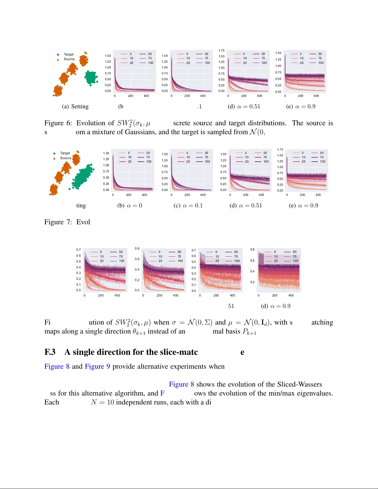
Con v er gence Rates for Distrib ution Matching with Sliced Optimal T ransport Gauthier Thurin * 1 , Claire Boyer 2 , and Kimia Nadjahi 1 1 CNRS, ENS P aris, F rance 2 LMO, Universit ´ e P aris-Saclay , Orsay , F rance ; Institut univer sitair e de F rance Abstract W e study the slice-matching scheme, an efﬁcient iterative method for distrib ution match- ing based on sliced optimal transport. W e in vestigate con vergence to the tar get distrib ution and deri ve quantitati ve non-asymptotic rates. T o this end, we establish Łojasiewicz-type inequal- ities for the Sliced-W asserstein objective. A key challenge is to control along the trajectory the constants in these inequalities. W e sho w that this becomes tractable for Gaussian distri- butions. Speciﬁcally , eigen values are controlled when matching along random orthonormal bases at each iteration. W e complement our theory with numerical experiments and illus- trate the predicted dependence on dimension and step-size, as well as the stabilizing ef fect of orthonormal-basis sampling. K eywords: distribution matching, Sliced-W asserstein distance, computational optimal trans- port, non-con ve x optimization, stochastic gradient descent. 1 Intr oduction Many problems in modern machine learning require comparing and matching probability distribu- tions, as in generati ve modeling ( Marzouk et al. , 2016 ; Grenioux et al. , 2023 ), density estimation ( W ang and Marzouk , 2022 ; Irons et al. , 2022 ) or domain adaptation ( Courty et al. , 2016 ). The goal is typically to transform a source distrib ution in order to match a more complex target distribution. Distribution matching and optimal transport. Distribution matching can be naturally formal- ized through optimal transport (O T), which provides both a geometrically meaningful distance between probability measures and, when it exists, a transport map pushing a source distribution σ to a target distribution µ ( V illani , 2008 ; Ambrosio and Sav ar ´ e , 2007 ). O T -based methods hav e led to major theoretical and algorithmic adv ances across machine learning, image processing and scientiﬁc computing ( Pe yr ´ e et al. , 2019 ; Santambrogio , 2015 ). Howe ver , computing O T maps is in general expensi ve both computationally and statistically ( H ¨ utter and Rigollet , 2021 ; Chewi et al. , 2024 ). * Corresponding author: gthurin@mail.di.ens.fr . Python codes are av ailable at https://github. com/gauthierthurin/SlicedMaps . 1 Iterative approaches and measur e interpolations. The high cost of O T has motiv ated alter- nati ve approaches that decompose the transport problem into simpler subproblems. A ke y idea is to build an interpolation between σ and µ through a sequence of elementary transformations, rather than estimating a single global transport map. This idea underlies many iterati ve correction schemes: although each step may only partially reduce the discrepanc y between σ and µ , their composition is expected to gradually align them. Among all possible interpolations, the McCann interpolation ( McCann , 1997 ) plays a distinguished theoretical role, as it corresponds to geodesics in W asserstein space, but it is rarely tractable. A generic iterati ve sequence of measures that mimics McCann’ s interpolation can be constructed through b σ k +1 =  (1 − γ k ) Id + γ k b T k  ♯ b σ k , (1) where b T k is an approximate transport map from b σ k to µ , ( γ k ) k a sequence of step sizes. Here, T ♯ σ denotes the pushforward of σ by the function T : if X ∼ σ , then T ( X ) ∼ T ♯ σ . Dif ferent choices for b T k hav e been proposed, such as entropy-regularized O T ( Kassraie et al. , 2024 ) and neural-network parameterizations in diffusion or ﬂow-based models ( Song et al. , 2021 ; Albergo et al. , 2025 ). In this work, we focus on sliced optimal transport, a computationally ef ﬁcient alternati ve that le verages one-dimensional projections ( Piti ´ e et al. , 2007 ; Rabin et al. , 2011 , 2012 ). Sliced optimal transport and slice-matching maps. The Sliced-W asserstein distance (SW) compares two distrib utions by projecting them onto one-dimensional subspaces and averaging the resulting W asserstein distances ( Rabin et al. , 2011 , 2012 ). Thanks to its scalability and simple im- plementation, SW has attracted growing interest in large-scale applications, including generati ve modeling ( Deshpande et al. , 2019 ; W u et al. , 2019 ; Liutkus et al. , 2019 ; Kolouri et al. , 2018 ; Dai and Seljak , 2021 ; Coeurdoux et al. , 2022 ; Du et al. , 2023 ). This empirical success has in turn moti- v ated theoretical w ork on the geometry induced by sliced O T , sample comple xity , and con ver gence properties of associated algorithms ( Nadjahi et al. , 2019 , 2020 ; Manole et al. , 2022 ; T anguy , 2023 ; T anguy et al. , 2025 ; Li and Moosmueller , 2023 ; V authier et al. , 2025 ). Although sliced O T does not directly provide transport maps or geodesics ( Kitagaw a and T akatsu , 2024 ; Park and Slep ˇ ce v , 2025 ), sev eral constructions hav e been proposed in this spirit ( Liu et al. , 2025 ; Mahey et al. , 2023 ). In particular , slice-matching maps ( Piti ´ e et al. , 2007 ; Li and Moosm ¨ uller , 2024 ) correspond to W asserstein gradients of the SW functional ( Li and Moos- mueller , 2023 ). For a direction θ ∈ S d − 1 , let σ θ and µ θ denote the push-forwards of σ and µ by the projection x 7→ ⟨ x, θ ⟩ . Denoting by T µ θ σ θ : R → R the univ ariate optimal transport map from σ θ to µ θ , the associated slice-matching map is deﬁned by T σ,θ ( x ) = x +  T µ θ σ θ ( θ T x ) − θ ⊤ x  θ . (2) Since the probability mass is transported along a single direction, T σ,θ does not transport σ to µ . The Iterative Distribution T ransfer (IDT) algorithm ( Piti ´ e et al. , 2007 ) therefore constructs an iterati ve composition of slice-matching maps, corresponding to ( 1 ) with constant step sizes γ k = 1 . Using random directions θ at each iteration, this procedure is expected to gradually push σ to µ and has been successfully applied in practice. 2 Related works. The IDT algorithm ( Piti ´ e et al. , 2007 ) was introduced before the Sliced-W asserstein distance ( Rabin et al. , 2011 , 2012 ) and was later interpreted as an iterati ve sliced O T procedure. Early works established con vergence of the IDT iterates when the target is the standard Gaus- sian distribution and studied its continuous-time limit, often referred to as the Sliced-W asserstein ﬂow ( Piti ´ e et al. , 2007 ; Bonnotte , 2013 ). More recently , Cozzi and Santambrogio ( 2025 ) prov ed con ver gence of SW ﬂo ws to the isotropic Gaussian. Relativ ely few results are a vailable on the con ver gence of sliced O T procedures beyond the Gaussian setting. A more general analysis is conducted in Li and Moosmueller ( 2023 ), which reinterprets IDT as a stochastic gradient descent method (SGD) on SW and accounts for time discretization and randomness in the sampled direc- tions. They prov e asymptotic con vergence of the discrete-time dynamics under strong assumptions, notably that the iterates remain in a compact set containing no other critical points than the target measure. In parallel, se veral works hav e studied SW as a loss between discrete measures and highlight the existence of nontri vial critical points, which moti vate noisy or regularized variants of SGD ( T anguy et al. , 2024 , 2025 ; V authier et al. , 2025 ). Contributions. The main goal of this paper is to establish con vergence rates for the slice-matching scheme ( Li and Moosmueller , 2023 ). Our approach is based on identifying Polyak–Łojasiewicz (PL) inequalities for the Sliced-W asserstein objectiv e, which bound the loss by the squared norm of its W asserstein gradient. These inequalities imply quantitativ e con ver gence rates to the target distribution. The main technical challenge is that the associated constants depend on lo wer and upper bounds on the density of the iterates, which are dif ﬁcult to control along the trajectory . W e address this difﬁculty within the class of elliptic distrib utions, for which slice-matching maps are linear . In this regime, controlling the density of the iterates amounts to controlling the eigen values of their cov ariance matrices. When the target distribution is isotropic, we sho w that these eigen values can be controlled in e xpectation, which in turn yields e xplicit con vergence rates. Crucially , such spectral control holds from the very ﬁrst iteration when the updates use random orthonormal bases of directions. This stands in contrast with the single-direction setting, where the lack of orthogonality leads to larger ﬂuctuations in the co variance structure before stabilization. Structure. Section 2 introduces the mathematical framework. Preliminary con ver gence results to critical points are discussed in Section 3 . Section 4 presents our main results on Łojasiewicz- and PL-type inequalities and on the control of the associated constants. Numerical experiments are reported in Section 5 , follo wed by a conclusion. T echnical proofs are deferred to the appendices. Notation. For any probability measure ν on R d , let M 2 ( ν ) = R R d ∥ x ∥ 2 d ν ( x ) be its second mo- ment. P 2 ( R d ) refers to the set of measures with a ﬁnite second moment and P 2 ,ac ( R d ) ⊂ P 2 ( R d ) is the set of absolutely continuous measures with respect to the Lebesgue measure. W e denote the Euclidean norm and inner product on R d by ∥ · ∥ and ⟨· , ·⟩ . For ν ∈ P 2 ( R d ) , we deﬁne L 2 ( ν ) = { f : R d → R d : R R d ∥ f ( x ) ∥ 2 d ν ( x ) ≤ + ∞} , and for f , g ∈ L 2 ( ν ) , ⟨ f , g ⟩ ν = R R d ⟨ f ( x ) , g ( x ) ⟩ d ν ( x ) , ∥ f ∥ ν = p ⟨ f , f ⟩ ν . Let S d − 1 = { θ ∈ R d : ∥ θ ∥ = 1 } be the unit sphere in R d . For any θ ∈ S d − 1 , π θ : R d → R is the projection π θ ( x ) = ⟨ x, θ ⟩ . Finally , λ i ( A ) refers to the i -th smallest eigen value of a matrix A , with λ min ( A ) the smallest and λ max ( A ) the lar gest. 3 2 Backgr ound on the Slice-Matching Scheme W e begin by re vie wing the deﬁnition of optimal transport and its properties for one-dimensional measures, which moti v ates slicing. Let T µ σ denote the O T map from σ to µ , deﬁned as a minimizer in the W asserstein distance: W 2 2 ( σ, µ ) = inf T : T ♯ σ = µ E X ∼ σ   X − T ( X )   2 . In dimension one, the optimal transport map admits a closed-form expression, T µ σ = F − 1 µ ◦ F σ , where F ρ is the cumu- lati ve distribution function of ρ ∈ P 2 ( R ) . This moti v ates the deﬁnition of the Sliced-W asserstein distance, which av erages one-dimensional W asserstein distances ov er random projections: S W 2 2 ( σ, µ ) = Z S d − 1 W 2 2 ( σ θ , µ θ ) d U ( θ ) , where σ θ = ( π θ ) ♯ σ and µ θ = ( π θ ) ♯ µ , and U is the uniform distribution on S d − 1 . Slice-matching maps and scheme. W e now introduce the slice-matching construction that un- derlies the iterati ve scheme studied in this paper . Let µ ∈ P 2 ,ac ( R d ) be a target probability measure, and let P = [ θ 1 , . . . , θ d ] ∈ R d × d be an orthonormal basis of R d . For any direction θ ∈ S d − 1 , denote by t θ = T µ θ σ θ the one-dimensional optimal transport map pushing the projected measure σ θ onto µ θ . Rather than transporting mass along a single direction, we simultaneously match d orthogonal one-dimensional projections. This leads to the deﬁnition of the (matrix-)slice-matching map ∀ x ∈ R d , T σ,P ( x ) = x + P      t θ 1 ( θ ⊤ 1 x ) − θ ⊤ 1 x t θ 2 ( θ ⊤ 2 x ) − θ ⊤ 2 x . . . t θ d ( θ ⊤ d x ) − θ ⊤ d x      = d X i =1 t θ i ( θ ⊤ i x ) θ i , (3) where the last equality follo ws from the fact that P is an orthonormal basis. Using se veral or - thogonal directions at each iteration has been observed to signiﬁcantly improv e both stability and empirical performance ( Piti ´ e et al. , 2007 ; Bonneel et al. , 2015 ; Li and Moosmueller , 2023 ). From a theoretical standpoint, matrix-slice-matching maps enjoy a moment-matching property ( Li and Moosm ¨ uller , 2024 , Proposition 3.6), which will play a central role in our analysis: E Y ∼ ( T σ,P ) ♯ σ [ Y ] = E Y ∼ µ [ Y ] , M 2  ( T σ,P ) ♯ σ  = M 2 ( µ ) . The slice-matc hing scheme , main focus of this paper , is deﬁned as follo ws: Starting from an initial distribution σ 0 = σ ∈ P 2 ,ac ( R d ) , the iterates are gi ven by ∀ k ≥ 0 , σ k +1 =  (1 − γ k ) Id + γ k T σ k ,P k +1  ♯ σ k , (4) where ( P k ) k ≥ 1 is an i.i.d. sequence of random orthonormal bases drawn according to the Haar measure on R d , and ( γ k ) k ≥ 0 consist of positi ve step sizes satisfying the Robbins–Monro conditions X k ≥ 0 γ k = + ∞ , X k ≥ 0 γ 2 k < + ∞ . (5) 4 Stochastic gradient descent perspecti ve. The slice-matching scheme admits a natural interpre- tation as a stochastic gradient descent procedure in the 2 -W asserstein space for a Sliced-W asserstein loss ( Li and Moosmueller , 2023 ). Speciﬁcally , consider the v ariational problem min σ ∈P 2 ( R d ) F ( σ ) , with F ( σ ) = d 2 S W 2 2 ( σ, µ ) . (6) For P = [ θ 1 , . . . , θ d ] an orthonormal basis of R d , deﬁning F ( σ, P ) = 1 2 P d ℓ =1 W 2 2 ( σ θ ℓ , µ θ ℓ ) , one has the decomposition F ( σ ) = E P  F ( σ , P )  , where the expectation is taken with respect to P 1 . Both F and F ( · , P ) depend on the target measure µ , a dependence that we omit in the notation for simplicity . The W asserstein gradient of the random functional F ( · , P ) is gi ven by ∇ W 2 F ( σ , P ) = Id − T σ,P , and provides an unbiased estimator of the full W asserstein gradient: E P  ∇ W 2 F ( σ , P )  = ∇ W 2 F ( σ ) , see Rabin et al. ( 2011 ); Bonnotte ( 2013 ); Li and Moosmueller ( 2023 ); Cozzi and Santambrogio ( 2025 ) and Proposition B.1 (Appendix B ). As a consequence, the slice-matching iteration ( 4 ) can be re written as a stochastic gradient descent update in W asserstein space. For any k ≥ 0 , σ k +1 =  Id − γ k ( Id − T σ k ,P k +1 )  ♯ σ k =  Id − γ k ∇ W 2 F ( σ k , P k +1 )  ♯ σ k . (7) For completeness, Appendix A recalls basic notions of dif ferentiation in W asserstein space. Bounded gradients. Cozzi and Santambrogio ( 2025 ) show that second-order moments are bounded along the Sliced-W asserstein ﬂow . In our discrete time setting that incorporates stochastic choices of directions P k +1 , we can sho w that the same holds as a result of the aforementioned moment- matching property of slice-matching maps (see Proposition B.8 , Appendix B ). Combining this with ∥∇ W 2 F ( σ ) ∥ 2 σ ≤ 2 F ( σ ) (by Jensen’ s inequality; see Proposition B.1 , Appendix B ), one has ∀ k ≥ 0 , ∥∇ W 2 F ( σ k ) ∥ 2 σ k ≤ 2 F ( σ k ) ≤ 4M 2 ( µ ) . Smoothness and non-conv exity . A ke y property for SGD is the smoothness of the objectiv e function. It is shown in V authier et al. ( 2025 ) (and recalled in Appendix B.2 ) that F is 1-smooth in P 2 ( R d ) endo wed with W 2 : for any σ 1 , σ 2 ∈ P 2 ( R d ) such that the O T map T σ 2 σ 1 exists, F ( σ 2 ) ≤ F ( σ 1 ) + ⟨∇ F ( σ 1 ) , T σ 2 σ 1 − Id ⟩ σ 1 + 1 2 W 2 2 ( σ 1 , σ 2 ) . (8) Smoothness alone, ho we ver , is not sufﬁcient to guarantee almost-sure conv ergence towards µ . In W asserstein spaces, con vergence rates typically rely on geodesic con vexity ( Ambrosio and Sa var ´ e , 2007 ), which F does not satisfy in general ( V authier et al. , 2025 ). Nev ertheless, con ver gence is observed in practice ( Piti ´ e et al. , 2007 ; Rabin et al. , 2011 ), which suggests that the optimization landscape remains highly structured, as studied in the next section. 1 This equality follows from the inv ariance of the Haar measure, which ensures that the marginal distrib ution of each direction θ ℓ is uniform on S d − 1 , ev en though the directions are not independent. 5 3 Pr eliminary Analysis: Con ver gence to Critical Points W e recall con ver gence results from Li and Moosmueller ( 2023 ) and deriv e new results about a ver - ages of gradient norms with standard proofs that use the smoothness property . Descent lemma. The follo wing lemma is a key recursion inequality that serves as a standard descent condition in stochastic optimization. The proof follo ws by the smoothness property ( 8 ) and direct computations, in the same fashion as for optimization o ver Euclidean spaces. Lemma 3.1 ( Li and Moosmueller ( 2023 ), Lemma A.1) . Let ( σ k ) k ≥ 1 be the iterates generated by the slice-matching sc heme ( 4 ) . Then, for any k ≥ 0 , E [ F ( σ k +1 ) |A k ] ≤ (1 + γ 2 k ) F ( σ k ) − γ k ∥∇ W 2 F ( σ k ) ∥ 2 σ k , (9) wher e A k is the σ -ﬁeld generated by ( P 1 , . . . , P k ) . Gi ven recursion ( 9 ) and step-sizes assumptions ( 5 ), a direct application of Robbins-Siegmund theorem ( Robbins and Siegmund , 1971 ) implies that ( F ( σ k )) k ≥ 0 con ver ges almost surely to a ﬁnite random v ariable, and that X k ≥ 1 γ k   ∇ W 2 F ( σ k )   2 σ k < + ∞ a.s. (10) An immediate byproduct is that a subsequence of ( ∥∇ W 2 F ( σ k ) ∥ σ k ) k ≥ 1 con ver ges almost surely to 0 , or equiv alently lim inf k → + ∞ ∥∇ W 2 F ( σ k ) ∥ σ k = 0 . Besides, ( ∥∇ W 2 F ( σ k ) ∥ σ k ) k ≥ 1 con ver ges almost surely to 0 if the sequence ( σ k ) k ≥ 1 remains in a compact subset of ( P 2 ,ac ( R d ) , W 2 ) ( Li and Moosmueller , 2023 , Theorem 2). This holds true for instance if σ 0 and µ are continuous and compactly supported, or under ﬁnite third-order moments ( Li and Moosmueller , 2023 , Remark 9). Under the additional assumption that ∇ F ( σ ) = 0 ⇐ ⇒ σ = µ, the limit of σ k must be µ almost surely . T o the best of our knowledge, the only known sufﬁcient condition for this equiv alence is that densities are strictly positi ve on their compact support ( Bonnotte , 2013 , Lemma 5.7.2). Con vergence Guarantees to Critical Points. The next proposition establishes con vergence to- ward a critical point using standard ar guments, up to a random reshuf ﬂing of the indices ( Ghadimi and Lan , 2013 ). This result is weaker than the almost sure con vergence σ k a.s. → µ from Li and Moosmueller ( 2023 , Theorem 2), but it has the beneﬁt of requiring no additional assumptions than the ones of Lemma 3.1 . Here, this means absolute continuity for σ and µ , although smoothness ( 8 ) holds in fact in the more difﬁcult setting of V authier et al. ( 2025 ) where ( σ k ) are discrete. In this case, the next tw o propositions could be extended. Proposition 3.2. F or any K ∈ N , let i ( K ) be a random index such that ∀ k ∈ { 1 , . . . , K } , P ( i ( K ) = k ) = 1 /K . Then, ( ∥∇ F ( σ i ( K ) ) ∥ 2 σ i ( K ) ) K ≥ 0 con ver ges in pr obability towar ds 0 , i.e. , ∀ ϵ > 0 , lim K → + ∞ P  ∥∇ F ( σ i ( K ) ) ∥ 2 σ i ( K ) > ϵ  = 0 . T urning to con vergence rates, assuming smoothness and boundedness of the iterates only yields the follo wing result, which concerns a weighted av erage of the gradients. 6 Proposition 3.3. F or a number K of iterations, deﬁne the weigths ω j = γ j / P K k =1 γ k , for any 0 ≤ j ≤ K , wher e ( γ j ) j ar e the chosen learning rates. Then, K X k =0 ω k E [ ∥∇ W 2 F ( σ k ) ∥ 2 σ k ] ≤ F ( σ 0 ) + 4M 2 ( µ ) P K k =0 γ 2 k P K k =0 γ k . (11) When choosing γ k = 1 / ( k + 1) α for 1 / 2 < α < 1 , considering that the numerator is bounded by a constant, Proposition 3.3 yields a rate of order K α − 1 , since P K k =0 γ k ≥ 1 1 − α ( K 1 − α − 1) . W e also emphasize that the bound ( 11 ) would tend to zero for a constant step-size γ k = 1 / √ K + 1 gi ven a ﬁnite time horizon K (as in Ghadimi and Lan , 2013 ; Khaled and Richt ´ arik , 2023 ). These propositions complement the related work by V authier et al. ( 2025 ) that also study con- ver gence tow ards critical points. Their setting is dif ferent in that the y consider a discrete source σ , a continuous target µ , a constant learning rate and their gradients are theoretically computed from all directions θ ∈ S d − 1 , as opposed to our stochastic gradients along ﬁnitely many directions. The con ver gence results obtained so far are standard for stochastic optimization of smooth losses with bounded gradients ( Bottou et al. , 2018 ; Dossal et al. , 2024 ). For completeness, proofs are pro vided in Appendix B.4 . In the remainder of this paper , we will assume appropriate continu- ity conditions, allo wing us to strengthen and extend the preceding results. 4 Con vergence Analysis under Łojasiewicz Inequalities This section is dev oted to the deriv ation of quantitativ e con ver gence rates for the slice-matching scheme. Our main result concerns Gaussian source and target measures. 4.1 Main r esult: con ver gence analysis f or Gaussian measur es Theorem 4.1. Assume σ = N (0 , Σ) and µ = N (0 , I d ) , where Σ ∈ R d × d is symmetric positive deﬁnite. Let γ k = 1 / ( k + 1) α with 1 / 2 < α < 1 . Then, ther e exists C > 0 suc h that for k ≥ 1 , E [ F ( σ k )] ≤ C k 2 α − 1 . The complete proof is deferred to Appendix E . The remainder of this section presents the main ingredients and is or ganized as follows. W e ﬁrst introduce a general framework sho wing ho w con- ver gence rates follow from a r andom P olyak–Łojasiewicz (PL) inequality along the trajectory . W e then discuss ho w such inequalities can be established in a static fashion under density bounds, and why propagating these bounds is difﬁcult in general. Finally , we sho w that the Gaussian struc- ture allo ws one to control the corresponding PL constants through spectral estimates on cov ariance matrices, which leads to Theorem 4.1 . 4.2 Step 1: Fr om (random) PL inequalities to rates Our starting point is a gradient–variance decomposition (see Appendix B.1 , Proposition B.1 ) which isolates Łojasie wicz-type inequalities as the ke y ingredient. Denoting T σ = E P [ T σ,P ] , one has 2 F ( σ ) = ∥∇ W 2 F ( σ ) ∥ 2 σ + E P  ∥ T σ − T σ,P ∥ 2 σ  . (12) 7 If the v ariance term is controlled by the squared W asserstein gradient norm, i.e. , if there exists s > 0 such that E P  ∥ T σ − T σ,P ∥ 2 σ  ≤ s 2 ∥∇ W 2 F ( σ ) ∥ 2 σ , then ( 12 ) yields a Polyak–Łojasie wicz inequality F ( σ ) ≤ B ∥∇ W 2 F ( σ ) ∥ 2 σ , B = 1+ s 2 2 , a standard condition to prov e con ver gence rates in noncon ve x optimization ( e.g . Garrigos and Go wer , 2023 ). This moti v ates the search for PL inequalities that hold along the iterates ( σ k ) k ≥ 0 with constants that can be controlled. W e formalize this requirement through the following random Łojasie wicz condition ( Kurdyka et al. , 2000 ; Attouch et al. , 2010 ). Assumption A. F or some τ ∈ { 1 , 2 } and any k ≥ 1 , F ( σ k ) τ ≤ B k ∥∇ W 2 F ( σ k ) ∥ 2 σ k with ( B k ) k ≥ 1 a sequence of positive random variables s.t. sup k ≥ 1 E [ B p k ] ≤ c p with c p ∈ (0 , + ∞ ) for all p ∈ N ∗ . By combining such inequalities along the trajectory with the descent recursion for F ( σ k ) (Lemma 3.1 ), we obtain the follo wing rates. Theorem 4.2. Consider Assumption A with τ = 1 . Choose the step sequence as γ k = 1 / ( k + 1) α with 1 / 2 < α < 1 . Then, for any k ≥ 1 , E [ F ( σ k )] ≲ 1 k 2 α − 1 . Alternatively , consider Assumption A with τ = 2 . F or p ≥ 2 α / (2 − 3 α ) , let γ = (2M 2 ( µ ) √ c p ) 3 / 2 . Let γ k = 1 / ( k + γ ) α with 1 / 2 < α < 2 / 3 . Then, for any k ≥ 1 , E [ F ( σ k )] ≲ 1 / ( k + γ ) 2 α − 1 . Only ﬁnitely many moments of B k are required for the analysis. More precisely , the proof requires sup k ≥ 1 E [ B p k ] < ∞ for some p > 4 α / (1 − α ) when τ = 1 , and for some p ≥ 2 α/ (2 − 3 α ) when τ = 2 . For simplicity of e xposition, Assumption A is stated with uniform bounds for all p ∈ N ∗ . Beyond the slice-matching setting, the proof strategy applies more generally to optimization schemes with smooth objecti ves, whose gradients are bounded and that satisfy Assumption A . The argument follows a standard template: one ﬁrst deriv es a descent recursion, and then applies an appropriate variant of Chung’ s lemma ( Chung , 1954 ; Jiang et al. , 2024 ). The main additional dif ﬁculty here is that the PL constant B k is random. W e address this by working on ev ents of the form { B k ≤ g − 1 k } where g k → 0 is chosen so that these e vents ev entually occur almost surely . Similar ar guments appear in Godichon-Baggioni ( 2019 , Theorem 4.2) and Bercu and Bigot ( 2021 , Theorem 3.6) to lev erage local strong con ve xity . The main remaining difﬁculty is therefore to verify Assumption A for the slice-matching iterates. 4.3 Step 2: Static PL inequalities and bounded densities In this section, we show that Łojasie wicz-type inequalities can be established in a static manner , i.e. , for ﬁx ed measures with uniformly bounded densities. 8 Gradient domination f or bounded densities. For notational simplicity , we identify any σ ∈ P 2 ,ac ( R d ) with its density . Giv en a reference measure ν ∈ P 2 ,ac ( R d ) , we consider the con venient setting of measures with uniformly bounded densities P ν,m,M ( R d ) = { σ ∈ P ( R d ) : mν ≤ σ ≤ M ν } , (13) for which the follo wing gradient-domination inequality can be obtained. Proposition 4.3. Assume that ν ∈ P 2 ,ac ( R d ) satisﬁes a P oincar ´ e inequality with constant C ν > 0 , i.e., for any f : R d → R such that ∥∇ f ∥ 2 ν < + ∞ , V ar ν ( f ) ≜ ∥ f − E ν [ f ] ∥ 2 ν ≤ C ν ∥∇ f ∥ 2 ν . Then, if µ ∈ P ν,m,M ( R d ) , for any σ ∈ P ν,m,M ( R d ) , F ( σ ) ≤ 2 C ν M m   ∇ W 2 F ( σ )   σ . The proof follo ws arguments similar to Chizat et al. ( 2025 , Lemma 3.3). Note that, combined with ∥∇ W 2 F ( σ ) ∥ 2 σ ≤ 2 F ( σ ) , we obtain the two-sided estimate ∥∇ W 2 F ( σ ) ∥ 2 σ / 2 ≤ F ( σ ) ≤ 2 C ν M m   ∇ W 2 F ( σ )   σ . In particular , ∇ W 2 F ( σ ) = 0 if and only if F ( σ ) = 0 , i.e. , σ = µ . W e therefore retrie ve a characterization of critical points by Bonnotte ( 2013 , Lemma 5.7.2), where compactness of the support is no longer required. PL inequality f or Gaussians. W e no w turn to the Gaussian setting, in which PL inequalities can be established. W e consider the class G m,M = { ρ Σ : Σ ∈ S d ++ , m I d ⪯ Σ ⪯ M I d } , (14) where ρ Σ = N (0 , Σ) , and S d ++ is the set of positiv e deﬁnite d × d matrices. The notation ⪯ refers to the Loewner partial order: for two symmetric matrices ( A, B ) , A ⪯ B if and only if B − A is positiv e semi-deﬁnite. Therefore, G m,M corresponds to Gaussian measures with uniformly bounded cov ariance eigen values. Proposition 4.4 (PL inequality on G m,M ) . Let σ = ρ Σ and µ = ρ Λ such that Σ , Λ ar e simultane- ously diagonalizable by an orthogonal matrix (i.e., co-diagonalizable). Assume ρ Σ , ρ Λ ∈ G m,M . Let C d = d ( d + 2) M /m . Then, F ( σ ) ≤ C d 2  1 + M m    ∇ W 2 F ( σ )   2 σ . (15) Proposition 4.4 is proved by adapting Chewi et al. ( 2020 , Theorem 19), which yields an inter- mediate inequality relating F ( σ ) and ∥∇ W 2 F ( σ ) ∥ for σ , µ ∈ G m,M (see Appendix C.2 ). W e then reﬁne it into a PL inequality by proving that, for co-diagonalizable co variances, W 2 2 ( ρ Σ , ρ Λ ) ≤ C d S W 2 2 ( ρ Σ , ρ Λ ) . (16) T o our knowledge, this is the ﬁrst comparison between W 2 and S W 2 with polynomial dimension dependence, instead of exponential dependence obtained in general settings, e .g. , Bonnotte ( 2013 , Theorem 5.1.5) and Carlier et al. ( 2025 ). This result may be of independent interest for other research problems in volving Gaussian distrib utions and the Bures-W asserstein metric. 9 From static inequalities to iterate stability . T o use Proposition 4.3 (or Proposition 4.4 ) in a con ver gence analysis, one must ensure that the iterates ( σ k ) k ≥ 0 remain in P ν,m,M ( R d ) (or G m,M ) with constants m, M uniform in k . Howe ver , if σ k satisﬁes such bounds, propagating them to σ k +1 is challenging. Indeed, since σ k +1 = S k # σ k , the change-of-v ariables formula yields σ k +1 ( S k ( x )) = σ k ( x ) det Jac [ S k ]( x ) . (17) Thus, propagating density bounds reduces to controlling det Jac [ S k ] , which typically requires strong regularity estimates on S k ; see e.g. , Caff arelli ( 1992 , 2000 ); Bobko v and Ledoux ( 2019 ); Park and Slep ˇ ce v ( 2025 ). One possible way to circumvent this difﬁculty in general settings is to introduce diffusion through entropic regularization ( Chizat et al. , 2025 ), but this leads to a differ - ent class of distribution-matching algorithms ( Liutkus et al. , 2019 ) and falls outside the scope of the present work. This observation moti v ates restricting attention to settings, such as the Gaussian case, where the relev ant constants can instead be controlled through an alternativ e, more tractable mechanism. 4.4 Step 3: Propagating PL constants along the trajectory in the Gaussian case T o apply Theorem 4.2 , it remains to verify Assumption A along the slice-matching trajectory , in the Gaussian setting. Slice-matching on the Bures-W asserstein manifold. W e begin by making the slice-matching updates explicit when matching two Gaussians. Let µ = ρ Λ and for a ﬁxed k ∈ N , σ k = ρ Σ k . Then, for any θ ∈ S d − 1 , the one-dimensional projections satisfy σ θ k = N (0 , θ ⊤ Σ θ ) , µ θ = N (0 , θ ⊤ Λ θ ) , and the corresponding optimal transport map between these marginals is linear and gi ven by T µ θ σ θ k ( s ) = τ θ s, with τ θ = p θ ⊤ Λ θ /θ ⊤ Σ θ . For P k +1 = [ θ 1 , · · · , θ d ] , deﬁne the diagonal matrix D k = diag ( τ θ 1 , . . . , τ θ d ) . The resulting slice- matching map T σ k ,P k +1 is also linear: ∀ x ∈ R d , T σ k ,P k +1 ( x ) = P k +1 D k P ⊤ k +1 x . As a consequence, the iterates remain Gaussian ( Altschuler et al. , 2021 ), i.e. , σ k = ρ Σ k , with cov ariance matrices e volving according to the follo wing recursion Σ k +1 = A k Σ k A ⊤ k , A k = (1 − γ k ) I d + γ k P k +1 D k P ⊤ k +1 . (18) Remark 4.5 (Centered Gaussians) . If γ 1 = 1 , the ﬁrst iteration enfor ces equality of the means of σ 1 and µ due to the moment matc hing pr operty of slice-matc hing maps ( Li and Moosm ¨ uller , 2024 , Pr oposition 3.6). Ther efor e, we may assume without loss of gener ality that σ and µ ar e center ed. Remark 4.6 (Elliptically contoured distrib utions) . All r esults of this section extend be yond the Gaussian case to elliptically contoured distrib utions. The ke y structural pr operty used thr oughout is the linearity of O T maps, which also holds in this br oader class ( Gelbrich , 1990 , Theor em 2.1). 10 Control of PL constants along the trajectory . The con vergence analysis relies on PL inequal- ities whose constants depend in versely on the smallest eigen v alue of the cov ariance matrices Σ k . Therefore, obtaining quantitativ e con ver gence rates requires uniform (in k ) control of 1 /λ min (Σ k ) , in expectation and with ﬁnite moments. W e thus proceed in three steps: (a) “Static” Łojasiewicz inequalities with random constants. Under the trace bound T r (Σ k ) ≤ Tr (Λ) ( Proposition B.8 ), one has λ min (Σ k ) ≤ λ max (Λ) . Consequently , Propositions 4.4 and C.1 yield, for τ ∈ { 1 , 2 } , F ( σ k ) τ ≤ B k   ∇ W 2 F ( σ k )   2 σ k , B k ≲ 1 λ min (Σ k ) . (19) Thus, the PL constant along the trajectory is random and may deteriorate if λ min (Σ k ) becomes small, which moti v ates a quantitati ve control of this quantity . (b) Recursion on λ min (Σ k +1 ) . W e e xploit the explicit cov ariance update ( 18 ). W e show that for any k ≥ 0 , there exists a direction θ i among the columns of P k +1 such that ( Proposition D.1 ) p λ min (Σ k +1 ) ≥ p λ min (Σ k )  1 − γ k + γ k τ θ i  , τ θ i = s θ ⊤ i Λ θ i θ ⊤ i Σ k θ i . (20) Since Σ 0 ≻ 0 and Λ ≻ 0 , it holds by induction that λ min (Σ k ) > 0 for all ﬁnite k . Hence, the PL inequality in Proposition 4.4 is well-deﬁned along the trajectory . (c) Moment control of 1 /λ min (Σ k ) . W e now le verage the recursion ( 20 ) to bound 1 /λ min (Σ k ) in expectation. A sufﬁcient condition is pro vided by Proposition D.4 : for some p ≥ 1 , E " X k ≥ 0 γ k E θ  θ ⊤ Σ k θ θ ⊤ Λ θ  p − 1  # < ∞ . (21) W e are able to verify ( 21 ) in the isotropic tar get case Λ = I d , although our numerical experi- ments suggest that ( 21 ) is v eriﬁed for more general target cov ariances. More precisely , for any p ∈ N ∗ , sup k ≥ 1 E [ λ min (Σ k ) − p ] < ∞ when Λ = I d ( Proposition D.2 ). Combining the PL inequality ( 19 ) with the abo ve moment bounds sho ws that Assumption A holds along the Gaussian slice-matching trajectory . Applying Theorem 4.2 then yields the con ver gence rate stated in Theorem 4.1 . 5 Numerical Experiments 5.1 Matching Gaussians W e implement the slice-matching scheme with source σ = N (0 , Σ) and target µ = N (0 , I d ) to illustrate our theoretical insights from Section 4 . The updates are computed exactly following the explicit cov ariance recursion ( 18 ). W e run the algorithm for different dimensions d ∈ [5 , 100] and step-size schedules γ k = ( k + 1) − α with α ∈ [0 , 1) . For each ( d, α ) , we perform N = 10 independent runs (independent initializations of Σ ), and we track the loss S W 2 2 ( σ k , µ ) (to verify con ver gence) and the extreme eigen values λ min (Σ k ) , λ max (Σ k ) . 11 (a) Setting 0 200 400 0.0 0.2 0.4 0.6 0.8 5 10 20 50 75 100 (b) α = 0 0 200 400 0.0 0.1 0.2 0.3 0.4 0.5 0.6 5 10 20 50 75 100 (c) α = 0 . 1 0 200 400 0.0 0.2 0.4 0.6 5 10 20 50 75 100 (d) α = 0 . 51 0 200 400 0.0 0.2 0.4 0.6 0.8 5 10 20 50 75 100 (e) α = 0 . 9 Figure 1: Ev olution of S W 2 2 ( σ k , µ ) when σ = N (0 , Σ) and µ = N (0 , I d ) 0 100 200 300 400 500 0.5 1.0 1.5 2.0 5 10 20 50 75 100 (a) α = 0 0 100 200 300 400 500 0.5 1.0 1.5 2.0 5 10 20 50 75 100 (b) α = 0 . 1 0 100 200 300 400 500 0.5 1.0 1.5 2.0 5 10 20 50 75 100 (c) α = 0 . 51 0 100 200 300 400 500 0.5 1.0 1.5 2.0 5 10 20 50 75 100 (d) α = 0 . 9 Figure 2: Minimum and maximum eigen values of Σ k when σ = N (0 , Σ) and µ = N (0 , I d ) Con vergence and impact of ( d, α ) . Figure 1 reports S W 2 2 ( σ k , µ ) as a function of the iteration k . For all tested dimensions d , the loss decreases, indicating con ver gence of the iterates toward the target measure. As d increases, the decay becomes slower , in agreement with our theoreti- cal results, since the constants in our bounds scale polynomially with d . Similarly , the extreme eigen values con ver ge to 1, which conﬁrms that Σ k becomes I d . Figure 1 also shows that smaller v alues of α ( i.e . , more aggressiv e step sizes) yield f aster empirical con ver gence, with α ∈ { 0 , 0 . 1 } typically performing best. This beha vior is not captured by our non-asymptotic analysis, deriv ed for α > 0 . 5 . Extending the theory to values of α close to 0 remains an open problem. Eigen value contr ol. A key ingredient in our proof is to control λ min (Σ k ) along the trajectory in order to verify Assumption A . In the isotropic target case µ = N (0 , I d ) , the theory predicts that once the second-moment bound M 2 ( σ k ) ≤ M 2 ( µ ) holds, which happens from the ﬁrst itera- tion ( Proposition B.8 ), the eigen values remain uniformly bounded ov er k ( Proposition D.2 ). This behavior can be observed in Figure 3 : the extreme eigenv alues settle in a ﬁxed range from the ﬁrst iteration. W e emphasize that this behavior is due the moment-matching property inherent to the choice of an orthonormal basis P k +1 at each iteration. Another v ariant samples a single θ k +1 ∈ S d − 1 per iteration and updates only along that direction. The resulting extreme eigen val- ues are shown in Figure 3 , and exhibit larger ﬂuctuations before stabilizing, which correlates with slo wer loss decay . The beneﬁt of random orthonormal bases is consistent with recent work on sampling strategies in sliced O T ( Sisouk et al. , 2025 ). 12 0 20 40 60 80 100 0.25 0.50 0.75 1.00 1.25 1.50 1.75 P (a) α = 0 0 20 40 60 80 100 0.5 1.0 1.5 2.0 P (b) α = 0 . 1 0 20 40 60 80 100 0.4 0.6 0.8 1.0 1.2 1.4 P (c) α = 0 . 51 0 20 40 60 80 100 0.25 0.50 0.75 1.00 1.25 1.50 1.75 P (d) α = 0 . 9 Figure 3: Comparison of sampling strategies: single direction θ k +1 or orthonormal basis P k +1 . W e report λ min (Σ k ) and λ max (Σ k ) with σ = N (0 , Σ) , µ = N (0 , I d ) , d = 5 . T arget Source (a) Setting 0 200 400 0.0 2.5 5.0 7.5 10.0 12.5 15.0 5 10 20 50 75 100 (b) α = 0 0 200 400 0 2 4 6 8 10 12 5 10 20 50 75 100 (c) α = 0 . 1 0 200 400 0 2 4 6 8 10 12 14 5 10 20 50 75 100 (d) α = 0 . 51 0 200 400 0 2 4 6 8 10 12 14 5 10 20 50 75 100 (e) α = 0 . 9 Figure 4: Evolution of S W 2 2 ( σ k , µ ) for discrete source and target distributions. The source and target samples are distrib uted from Gaussian mixtures. 5.2 Bey ond the Gaussian-to-Gaussian Setting Figure 4 considers discrete empirical distrib utions of n = 500 samples. In each run, the source and tar get are sampled from a Gaussian mixture with randomly-generated mixture components. W e plot S W 2 2 ( σ k , µ ) ov er iterations for N = 10 independent runs, across the same dimensions and step-size schedules as in the Gaussian setting. W e observe the same trends: the loss decreases for all d , con ver gence slows down as d increases, and smaller values of α typically yield faster con ver gence. It is worth noting that α = 0 . 1 outperforms α = 0 in our experiments, which illustrates the interest of slice-matching algorithm (where ( γ k ) is decaying) o ver IDT (where γ k = 1 ). W e provide additional experiments on empirical measures in Appendix F . While these discrete settings are not co vered by our theory , the empirical con vergence suggests that regularity may hold more broadly , despite identiﬁed technical issues ( T anguy et al. , 2025 ; V authier et al. , 2025 ). 6 Conclusion and P erspectives W e established con vergence rates for the slice-matching algorithm through Łojasiewicz-type in- equalities for the Sliced-W asserstein objectiv e. W e sho w that controlling the associated constants is tractable in the Gaussian (or elliptic) setting when sampling random orthonormal bases. A main limitation is that our e xplicit rate requires an isotropic Gaussian target, similarly to Cozzi and San- tambrogio ( 2025 ). Extending the theory to general Gaussian targets and non-elliptic distrib utions remains open. A promising direction is to introduce regularization ( e.g. , diffusi ve terms) to help maintain re gularity along the dynamics ( Liutkus et al. , 2019 ; T anguy et al. , 2025 ; Chizat et al. , 13 2025 ). Finally , our e xperiments show faster con ver gence with orthonormal bases of directions and step-size schedules γ k = 1 / ( k + 1) α with small α . The latter regime is not covered by our theo- rems and may require tools beyond decreasing-step stochastic approximation, for example Markov chains ( Dieule veut et al. , 2020 ). Acknowledgments This work beneﬁted from state aid managed by the National Research Agency ANR-23-IA CL- 0008 under France 2030, for the project PR[AI]RIE-PSAI. Refer ences Y oussef Marzouk, T arek Moselhy , Matthe w Parno, and Alessio Spantini. Sampling via Measure T ransport: An Introduction, pages 1–41. Springer International Publishing, Cham, 2016. ISBN 978-3-319-11259-6. doi: 10.1007/978- 3- 319- 11259- 6 23- 1. URL https://doi.org/10. 1007/978- 3- 319- 11259- 6_23- 1 . Louis Grenioux, Alain Oli viero Durmus, Eric Moulines, and Marylou Gabri ´ e. On sampling with approximate transport maps. In Andreas Krause, Emma Brunskill, K yunghyun Cho, Barbara Engelhardt, Siv an Sabato, and Jonathan Scarlett, editors, Proceedings of the 40th International Conference on Machine Learning, volume 202 of Proceedings of Machine Learning Research, pages 11698–11733. PMLR, 23–29 Jul 2023. URL https://proceedings.mlr. press/v202/grenioux23a.html . Sven W ang and Y oussef Marzouk. On minimax density estimation via measure transport. arXiv preprint arXi v:2207.10231, 2022. Nicholas J Irons, Meyer Scetbon, Soumik Pal, and Zaid Harchaoui. Triangular ﬂo ws for generati ve modeling: Statistical consistency , smoothness classes, and fast rates. In International Conference on Artiﬁcial Intelligence and Statistics, pages 10161–10195. PMLR, 2022. Nicolas Courty , R ´ emi Flamary , Devis T uia, and Alain Rakotomamonjy . Optimal transport for domain adaptation. IEEE transactions on pattern analysis and machine intelligence, 39(9):1853– 1865, 2016. C ´ edric V illani. Optimal transport: old and new, v olume 338. Springer , 2008. Luigi Ambrosio and Giuseppe Sav ar ´ e. Gradient ﬂows of probability measures. In Handbook of dif ferential equations: e volutionary equations, v olume 3, pages 1–136. Elsevier , 2007. Gabriel Peyr ´ e, Marco Cuturi, et al. Computational optimal transport: W ith applications to data science. Foundations and T rends® in Machine Learning, 11(5-6):355–607, 2019. Filippo Santambrogio. Optimal transport for applied mathematicians, volume 87. Springer , 2015. Jan-Christian H ¨ utter and Philippe Rigollet. Minimax estimation of smooth optimal transport maps. The Annals of Statistics, 49(2):1166–1194, 2021. 14 Sinho Che wi, Jonathan Niles-W eed, and Philippe Rigollet. Statistical optimal transport. arXi v preprint arXi v:2407.18163, 3, 2024. Robert J McCann. A con vexity principle for interacting gases. Adv ances in mathematics, 128(1): 153–179, 1997. Parnian Kassraie, Aram-Alexandre Pooladian, Michal Klein, James Thornton, Jonathan Niles- W eed, and Marco Cuturi. Progressi ve entropic optimal transport solvers. Advances in Neural Information Processing Systems, 37:19561–19590, 2024. Y ang Song, Jascha Sohl-Dickstein, Diederik P Kingma, Abhishek Kumar , Stefano Ermon, and Ben Poole. Score-based generativ e modeling through stochastic differential equations. In International Conference on Learning Representations, 2021. URL https://openreview. net/forum?id=PxTIG12RRHS . Michael Albergo, Nicholas M. Bofﬁ, and Eric V anden-Eijnden. Stochastic interpolants: A unifying frame work for ﬂows and dif fusions. Journal of Machine Learning Research, 26(209):1–80, 2025. URL http://jmlr.org/papers/v26/23- 1605.html . Franc ¸ ois Piti ´ e, Anil C Kokaram, and Rozenn Dahyot. Automated colour grading using colour distribution transfer . Computer V ision and Image Understanding, 107(1-2):123–137, 2007. Julien Rabin, Gabriel Peyr ´ e, Julie Delon, and Marc Bernot. W asserstein barycenter and its appli- cation to texture mixing. In International conference on scale space and variational methods in computer vision, pages 435–446. Springer , 2011. Julien Rabin, Gabriel Peyr ´ e, Julie Delon, and Marc Bernot. W asserstein barycenter and its ap- plication to texture mixing. In Alfred M. Bruckstein, Bart M. ter Haar Romeny , Alexander M. Bronstein, and Michael M. Bronstein, editors, Scale Space and V ariational Methods in Computer V ision, pages 435–446, Berlin, Heidelberg, 2012. Springer Berlin Heidelberg. ISBN 978-3-642- 24785-9. I. Deshpande, Y .-T . Hu, R. Sun, A. Pyrros, N. Siddiqui, S. K oyejo, Z. Zhao, D. Forsyth, and A. Schwing. Max-sliced wasserstein distance and its use for gans. In IEEE/CVF CVPR, 2019. Jiqing W u, Zhiwu Huang, Dinesh Acharya, W en Li, Janine Thoma, Danda Pani Paudel, and Luc V an Gool. Sliced wasserstein generati ve models. In Proceedings of the IEEE/CVF Conference on Computer V ision and Pattern Recognition, pages 3713–3722, 2019. Antoine Liutkus, Umut Simsekli, Szymon Majewski, Alain Durmus, and Fabian-Robert St ¨ oter . Sliced-wasserstein ﬂows: Nonparametric generativ e modeling via optimal transport and diffu- sions. In International Conference on machine learning, pages 4104–4113. PMLR, 2019. Soheil K olouri, Phillip E Pope, Charles E Martin, and Gustavo K Rohde. Sliced wasserstein auto- encoders. In International Conference on Learning Representations, 2018. Biwei Dai and Uros Seljak. Sliced iterativ e normalizing ﬂows. In Marina Meila and T ong Zhang, editors, Proceedings of the 38th International Conference on Machine Learning, volume 139 of Proceedings of Machine Learning Research, pages 2352–2364. PMLR, 18–24 Jul 2021. URL https://proceedings.mlr.press/v139/dai21a.html . 15 F . Coeurdoux, N. Dobigeon, and P . Chainais. Sliced-wasserstein normalizing ﬂows: be yond maximum likelihood training. In Proc. European Symposium on Artiﬁcial Neural Networks, Computational Intelligence and Machine Learning (ESANN), Bruges, Belgium, Oct. 2022. Chao Du, T ianbo Li, T ianyu Pang, Shuicheng Y an, and Min Lin. Nonparametric generativ e modeling with conditional sliced-Wasserstein ﬂows. In Andreas Krause, Emma Brunskill, K yunghyun Cho, Barbara Engelhardt, Si v an Sabato, and Jonathan Scarlett, editors, Proceedings of the 40th International Conference on Machine Learning, volume 202 of Proceedings of Machine Learning Research, pages 8565–8584. PMLR, 23–29 Jul 2023. URL https: //proceedings.mlr.press/v202/du23c.html . Kimia Nadjahi, Alain Durmus, Umut Simsekli, and Roland Badeau. Asymptotic guarantees for learning generativ e models with the sliced-wasserstein distance. Adv ances in Neural Information Processing Systems, 32, 2019. Kimia Nadjahi, Alain Durmus, L ´ ena ¨ ıc Chizat, Soheil K olouri, Shahin Shahrampour , and Umut Simsekli. Statistical and topological properties of sliced probability di ver gences. Advances in Neural Information Processing Systems, 33:20802–20812, 2020. T udor Manole, Si v araman Balakrishnan, and Larry W asserman. Minimax conﬁdence interv als for the Sliced W asserstein distance. Electronic Journal of Statistics, 16(1):2252 – 2345, 2022. doi: 10.1214/22- EJS2001. URL https://doi.org/10.1214/22- EJS2001 . Eloi T anguy . Con vergence of SGD for training neural networks with sliced wasserstein losses. T ransactions on Machine Learning Research, 2023. ISSN 2835-8856. URL https:// openreview.net/forum?id=aqqfB3p9ZA . Eloi T anguy , R ´ emi Flamary , and Julie Delon. Properties of discrete sliced wasserstein losses. Mathematics of Computation, 94(353):1411–1465, 2025. Shiying Li and Caroline Moosmueller . Measure transfer via stochastic slicing and matching. arXiv preprint arXi v:2307.05705, 2023. Christophe V authier , Quentin M ´ erigot, and Anna K orba. Properties of wasserstein gradient ﬂows for the sliced-wasserstein distance. arXi v preprint arXi v:2502.06525, 2025. Jun Kitagawa and Asuka T akatsu. Sliced optimal transport: is it a suitable replacement?, 2024. URL . Sangmin Park and Dejan Slep ˇ ce v . Geometry and analytic properties of the sliced wasserstein space. Journal of Functional Analysis, 289(7):110975, 2025. Xinran Liu, Rocio Diaz Martin, Y ikun Bai, Ashkan Shahbazi, Matthew Thorpe, Akram Aldroubi, and Soheil K olouri. Expected sliced transport plans. In The Thirteenth International Conference on Learning Representations, 2025. URL https://openreview.net/forum?id= P7O1Vt1BdU . 16 Guillaume Mahey , Laetitia Chapel, Gilles Gasso, Cl ´ ement Bonet, and Nicolas Courty . Fast opti- mal transport through sliced generalized wasserstein geodesics. In Thirty-sev enth Conference on Neural Information Processing Systems, 2023. URL https://openreview.net/ forum?id=n3XuYdvhNW . Shiying Li and Caroline Moosm ¨ uller . Approximation properties of slice-matching operators. Sampling Theory , Signal Processing, and Data Analysis, 22(1):15, 2024. Nicolas Bonnotte. Unidimensional and ev olution methods for optimal transportation. PhD thesis, Uni versit ´ e Paris Sud-P aris XI; Scuola normale superiore (Pise, Italie), 2013. Giacomo Cozzi and Filippo Santambrogio. Long-time asymptotics of the sliced-wasserstein ﬂow . SIAM Journal on Imaging Sciences, 18(1):1–19, 2025. doi: 10.1137/24M1656414. URL https://doi.org/10.1137/24M1656414 . Eloi T anguy , R ´ emi Flamary , and Julie Delon. Reconstructing discrete measures from projections. consequences on the empirical sliced wasserstein distance. Comptes Rendus. Math ´ ematique, 362(G10):1121–1129, 2024. Nicolas Bonneel, Julien Rabin, Gabriel Peyr ´ e, and Hanspeter Pﬁster . Sliced and radon wasserstein barycenters of measures. Journal of Mathematical Imaging and V ision, 51(1):22–45, 2015. Herbert Robbins and Da vid Siegmund. A con vergence theorem for non negati ve almost super - martingales and some applications. In Optimizing methods in statistics, pages 233–257. Else- vier , 1971. Saeed Ghadimi and Guanghui Lan. Stochastic ﬁrst-and zeroth-order methods for noncon vex stochastic programming. SIAM journal on optimization, 23(4):2341–2368, 2013. Ahmed Khaled and Peter Richt ´ arik. Better theory for SGD in the nonconv ex world. T ransactions on Machine Learning Research, 2023. ISSN 2835-8856. URL https://openreview. net/forum?id=AU4qHN2VkS . Survey Certiﬁcation. L ´ eon Bottou, Frank E Curtis, and Jorge Nocedal. Optimization methods for large-scale machine learning. SIAM revie w, 60(2):223–311, 2018. Charles Dossal, Samuel Hurault, and Nicolas P apadakis. Optimization with ﬁrst order algorithms. arXi v preprint arXi v:2410.19506, 2024. Guillaume Garrigos and Robert M Go wer . Handbook of con vergence theorems for (stochastic) gradient methods. arXiv preprint arXi v:2301.11235, 2023. Krzysztof Kurdyka, T adeusz Mostowski, and Adam Parusi ´ nski. Proof of the gradient conjecture of r . thom. Annals of Mathematics, pages 763–792, 2000. H ´ edy Attouch, J ´ er ˆ ome Bolte, Patrick Redont, and Antoine Soubeyran. Proximal alternating mini- mization and projection methods for noncon ve x problems: An approach based on the kurdyka- łojasie wicz inequality . Mathematics of operations research, 35(2):438–457, 2010. 17 Kai Lai Chung. On a stochastic approximation method. The Annals of Mathematical Statistics, pages 463–483, 1954. Li Jiang, Xiao Li, Andre Milzarek, and Junwen Qiu. A generalized v ersion of chung’ s lemma and its applications, 2024. URL . Antoine Godichon-Baggioni. Lp and almost sure rates of con ver gence of av eraged stochastic gradient algorithms: locally strongly con vex objective. ESAIM: Probability and Statistics, 23: 841–873, 2019. Bernard Bercu and J ´ er ´ emie Bigot. Asymptotic distribution and con ver gence rates of stochastic algorithms for entropic optimal transportation between probability measures. The Annals of Statistics, 49(2):968 – 987, 2021. doi: 10.1214/20- A OS1987. URL https://doi.org/ 10.1214/20- AOS1987 . L ´ ena ¨ ıc Chizat, Maria Colombo, and Xavier Fern ´ andez-Real. Con vergence of drift-diffusion pdes arising as wasserstein gradient ﬂows of con vex functions. arXi v preprint 2025. Sinho Che wi, T yler Maunu, Philippe Rigollet, and Austin J Stromme. Gradient descent algo- rithms for bures-w asserstein barycenters. In Conference on Learning Theory, pages 1276–1304. PMLR, 2020. Guillaume Carlier , Alessio Figalli, Quentin M ´ erigot, and Y i W ang. Sharp comparisons be- tween sliced and standard 1 -wasserstein distances, 2025. URL 2510.16465 . Luis A Caff arelli. The regularity of mappings with a con vex potential. Journal of the American Mathematical Society, 5(1):99–104, 1992. Luis A Caffarelli. Monotonicity properties of optimal transportation and the fkg and related in- equalities. Communications in Mathematical Physics, 214(3):547–563, 2000. Serge y Bobkov and Michel Ledoux. One-dimensional empirical measures, order statistics, and Kantorovich transport distances, v olume 261. American Mathematical Society , 2019. Jason Altschuler , Sinho Chewi, Patrik R Gerber , and Austin Stromme. A veraging on the b ures- wasserstein manifold: dimension-free con ver gence of gradient descent. Adv ances in Neural Information Processing Systems, 34:22132–22145, 2021. Matthias Gelbrich. On a formula for the l2 w asserstein metric between measures on euclidean and hilbert spaces. Mathematische Nachrichten, 147(1):185–203, 1990. K eanu Sisouk, Julie Delon, and Julien T ierny . A User’ s Guide to Sampling Strategies for Sliced Optimal T ransport. Transactions on Machine Learning Research, 2025. ISSN 2835-8856. Sur- ve y Certiﬁcation. A ymeric Dieuleveut, Alain Durmus, and Francis Bach. Bridging the gap between constant step size stochastic gradient descent and marko v chains. The Annals of Statistics, 48(3):1348–1382, 2020. 18 Y ann Brenier . Polar factorization and monotone rearrangement of v ector-v alued functions. Communications on pure and applied mathematics, 44(4):375–417, 1991. Juan Antonio Cuesta and Carlos Matr ´ an. Notes on the wasserstein metric in hilbert spaces. The Annals of Probability, pages 1264–1276, 1989. Martial Agueh and Guillaume Carlier . Barycenters in the wasserstein space. SIAM Journal on Mathematical Analysis, 43(2):904–924, 2011. Jianyu Ma. Absolute continuity of wasserstein barycenters on manifolds with a lower ricci curv a- ture bound. arXiv preprint arXi v:2310.13832, 2023. Beno ˆ ıt Kloeckner . A geometric study of wasserstein spaces: Euclidean spaces. Annali della Scuola Normale Superiore di Pisa-Classe di Scienze, 9(2):297–323, 2010. Beno ˆ ıt Bonnet. A pontryagin maximum principle in wasserstein spaces for constrained optimal control problems. ESAIM: Control, Optimisation and Calculus of V ariations, 25:52, 2019. Cl ´ ement Bonet, Th ´ eo Uscidda, Adam David, Pierre-Cyril Aubin-Franko wski, and Anna K orba. Mirror and preconditioned gradient descent in wasserstein space. In The Thirty-eighth Annual Conference on Neural Information Processing Systems, 2024. Nicolas Lanzetti, Sav erio Bolognani, and Florian D ¨ orﬂer . First-order conditions for optimization in the wasserstein space. SIAM Journal on Mathematics of Data Science, 7(1):274–300, 2025. Xingyu Zhou. On the fenchel duality between strong con vexity and lipschitz continuous gradient. arXi v preprint arXi v:1803.06573, 2018. R. T yrrell Rockafellar . Conv ex analysis. Princeton Univ ersity Press, 1970. Douglas P W iens. On moments of quadratic forms in non-spherically distrib uted v ariables. Statistics, 23(3):265–270, 1992. Alexander M Ostrowski. A quantitati ve formulation of sylvester’ s law of inertia. Proceedings of the National Academy of Sciences, 45(5):740–744, 1959. Eric Moulines and Francis Bach. Non-asymptotic analysis of stochastic approximation algorithms for machine learning. Advances in neural information processing systems, 24, 2011. 19 A Reminders on W asserstein space This appendix gathers existing results useful for optimization over the space of probability distri- butions. For further details, we refer the interesting reader to the classical references Ambrosio and Sav ar ´ e ( 2007 ); Santambrogio ( 2015 ). First, recall that, for ψ c ( y ) = inf x { 1 2 ∥ x − y ∥ 2 − ψ ( x ) } the c -transform of ψ , the dual of Kantorovich O T problem writes W 2 2 ( α, β ) = sup ψ ∈ L 1 ( α ) Z ψ d α + Z ψ c d β . (22) The solution of the latter is called the Kantorovich potential, and it is unique (up to translations) under ﬁniteness of second-order moments, with α giving no mass to d − 1 surfaces ( Santambrogio , 2015 , Theorem 1.22). A.1 Curv es and con vexity in W asserstein space The W asserstein space ( P 2 ( R d ) , W 2 ) is the space of square-integrable probability distrib utions endo wed with the W asserstein distance W 2 . A ﬁrst way to construct an absolutely continuous curve between tw o measures σ 0 and σ 1 is the ﬂat interpolation, gi ven, for t ∈ [0 , 1] , by σ t = (1 − t ) σ 0 + tσ 1 . (23) This con vex combination between densities ignores the geometry induced by the W asserstein dis- tance. In contrast, denoting by T σ 1 σ 0 the O T map from σ 0 to σ 1 , another interpolation is gi ven by σ t =  (1 − t ) Id + tT σ 1 σ 0  ♯ σ 0 . (24) Due to the fact that (1 − t ) Id + tT σ 1 σ 0 is the gradient of a con vex function, it is the solution of Monge O T problem ( Brenier , 1991 ; Cuesta and Matr ´ an , 1989 ). Hence, σ t corresponds to the shortest path between σ 0 and σ 1 , in the sense that ∀ 0 ≤ s ≤ t ≤ 1 , W 2 ( σ s , σ t ) = ( t − s ) W 2 ( σ 0 , σ 1 ) . While ( 23 ) corresponds to a mixture model between σ 0 and σ 1 , the interpolant ( 24 ) is more of a barycenter ( Agueh and Carlier , 2011 ; Rabin et al. , 2011 ) and it is a building block for gradient ﬂo ws in the W asserstein space ( Ambrosio and Sav ar ´ e , 2007 ). Interestingly enough, W 2 2 ( · , σ ) is strictly con vex along ( 23 ) as soon as σ is absolutely continuous ( Santambrogio , 2015 , Proposition 7.19). It is not hard to see that the same property holds for the Sliced-W asserstein distance, with arguments reminiscent to the ones of Ma ( 2023 , Proposition 2.10) for W asserstein barycenters. Such con ve xity along ( 23 ) must be understood with respect to the 2 -norm between densities. The analog along ( 24 ), with respect to the W asserstein distance, writes as follows. Deﬁnition A.1. F is geodesically α -con vex if, for all σ 0 , σ 1 ∈ P 2 ( R d ) and σ t = ((1 − t ) Id + tT σ 1 σ 0 ) ♯ σ 0 , F ( σ t ) ≤ (1 − t ) F ( σ 0 ) + t F ( σ 1 ) − α 2 t (1 − t ) W 2 2 ( σ 0 , σ 1 ) . 20 Unfortunately , the rev erse inequality holds for W 2 2 ( · , σ ) in general dimension ( Ambrosio and Sav ar ´ e , 2007 , Theorem 7.3.2), and a fortiori for the Sliced-W asserstein distance up to integration ov er the projection directions ( V authier et al. , 2025 , Appendix A.5). These facts are discussed in Lemma B.5 . The situation is very different in dimension d = 1 , due to the particular properties of ( P 2 ( R ) , W 2 ) . In this setting, the composition of O T maps preserves their monotonicity (hence the optimality) and W 2 re writes with Q 0 , Q 1 the quantile functions of σ 0 , σ 1 : W 2 2 ( σ 0 , σ 1 ) = Z 1 0 ∥ Q 0 ( t ) − Q 1 ( t ) ∥ 2 dt (25) or , equi v alently , W 2 2 ( σ 0 , σ 1 ) = ∥ T σ 0 ρ − T σ 1 ρ ∥ 2 ρ for any pi vot measure ρ ∈ P 2 ,ac ( R d ) . As a byproduct, the geodesics in ( 24 ) coincide with the generalized geodesics σ t =  (1 − t ) T σ 0 ρ + tT σ 1 ρ  ♯ ρ , and one can ﬁnd in Ambrosio and Sav ar ´ e ( 2007 , Chapter 9) that they verify the generalized parallelogram rule W 2 2 ( σ t , σ ) = (1 − t ) W 2 2 ( σ 0 , σ ) + tW 2 2 ( σ 1 , σ ) − t (1 − t ) W 2 2 ( σ 0 , σ 1 ) . (26) This can be easily veriﬁed by expanding the square in W 2 2 ( σ t , σ ) via ( 25 ) and using the tricks t 2 = t − t (1 − t ) and (1 − t ) 2 = (1 − t ) − t (1 − t ) , as in Kloeckner ( 2010 , Proposition 4.1). Next, we turn to dif ferentiation along geodesics. Unfortunately , ( 26 ) does not imply the same parallelogram identity for the Sliced-W asserstein distance, as it would require to identify a path σ t in R d along the map T : x 7→ R θ T µ θ σ θ ( x ) d U ( θ ) with all projected generalized geodesics σ θ t , which is not true. A.2 Differ entiation along geodesics W e borro w the dif ferential structure of ( P 2 ( R d ) , W 2 ) as described in e.g. , Bonnet ( 2019 ); Bonet et al. ( 2024 ); Lanzetti et al. ( 2025 ). The tangent space of P 2 ( R d ) at σ is deﬁned by T σ = {∇ ψ : ψ ∈ C ∞ c ( R d ) } , where the closure is taken with respect to the set of σ -square integrable functions from R d to R d , and where C ∞ c ( R d ) is the set of inﬁnitely dif ferentiable functions with compact support. Consider F : P 2 ( R d ) → R . At any σ ∈ P 2 ( R d ) such that F ( σ ) < + ∞ , the W asserstein gradient ∇ W 2 F ( σ ) is the unique vector in T σ verifying, for an y µ ∈ P 2 ( R d ) and any optimal coupling γ ∈ Π( σ, µ ) 2 , F ( µ ) = F ( σ ) + Z ⟨∇ W 2 F ( σ )( x ) , y − x ⟩ d γ ( x, y ) + o ( W 2 ( σ, µ )) . (27) One way to compute the W asserstein gradient is by taking ∇ W 2 F ( σ ) = ∇ δ F δ σ ( σ ) . for δ F δ σ ( σ ) the ﬁrst v ariation ( Santambrogio , 2015 , Deﬁnition 7.12) deﬁned as follows. Firstly , a measure ρ ∈ P 2 ,ac ( R d ) is r e gular for F if, for ev ery ρ ∈ P 2 ,ac ( R d ) with L ∞ density and compact support, F ((1 − t ) ρ + tρ ) < + ∞ for ev ery t ∈ [0 , 1] . With this at hand, if ρ is regular for F , the ﬁrst v ariation δ F δ ρ ( ρ ) veriﬁes d d t F ( ρ + tξ ) | t =0 = lim t → 0 F ( ρ + tξ ) − F ( ρ ) t = Z δ F δ ρ ( ρ )d ξ , 2 The set of couplings between σ and µ is Π( σ, µ ) = { π ∈ P 2 ( R d × R d ) : π ( A × R d ) = σ ( A ) , π ( R d × B ) = µ ( B ) } . 21 for all ξ = ρ − ρ with ρ ∈ P 2 ,ac ( R d ) with L ∞ density and compact support. The following useful remark is taken from ( Santambrogio , 2015 , Remark 7.14). Remark A.2. F or σ ∈ P 2 ,ac ( R d ) and F : ρ 7→ W 2 2 ( ρ, σ ) , any ρ ∈ P 2 ,ac ( R d ) is r e gular if and only if F ( ρ ) < + ∞ . Indeed, for every ρ ∈ P 2 ,ac ( R d ) , F ((1 − t ) ρ + tρ ) ≤ (1 − t ) F ( ρ ) + t F ( ρ ) by strict con vexity ( Santambr ogio , 2015 , Pr oposition 7.19). Hence, as soon as ρ is compactly supported, F ( ρ ) < + ∞ and ρ is r e gular if F ( ρ ) < + ∞ . The r ecipr ocal is immediate by taking t = 0 in the deﬁnition of a r e gular measure . When considering the W asserstein distance σ 7→ W 2 2 ( σ, µ ) , the ﬁrst variation is ψ , the Kan- torovich potential that is solution of ( 22 ) (Proposition 7.17, Santambrogio , 2015 ), and a similar statement holds for σ 7→ S W 2 2 ( σ, µ ) ( Cozzi and Santambrogio , 2025 ). W e discuss this in Proposi- tion B.1 . B Pr oofs of Sections 2 and 3 In this section, we detail the properties of the functional to be minimized. W e discuss differentia- bility and critical points, before turning to smoothness and boundedness of the gradient, the latter being a byproduct of boundedness of moments along the iterations. B.1 Differ entiability , critical points The ne xt proposition describes W asserstein gradients of our sliced objecti ve, as pre viously pro- vided in Bonnotte ( 2013 ); Cozzi and Santambrogio ( 2025 ). W e also detail simple properties of the gradient norm, that are important with the purpose of SGD. Proposition B.1. Given that µ ∈ P 2 ,ac ( R d ) is compactly supported, the W asserstein gradients of F ( · , θ ) and F at any σ ∈ P 2 ,ac ( R d ) compactly supported ar e given by ∇ W 2 F ( σ , P ) = Id − T σ,P and ∇ W 2 F ( σ ) = d Z θ ( Id − T µ θ σ θ ) ◦ π θ d U ( θ ) , wher e T µ θ σ θ denotes the one-dimensional O T map pushing σ θ to µ θ . It follows that ∥∇ W 2 F ( σ , P ) ∥ 2 σ = d X ℓ =1 W 2 2 ( σ θ ℓ , µ θ ℓ ) and ∥∇ W 2 F ( σ ) ∥ 2 σ ≤ dS W 2 2 ( σ, µ ) , that is ∥∇ W 2 F ( σ , P ) ∥ 2 σ = 2 F ( σ , P ) and ∥∇ W 2 F ( σ ) ∥ 2 σ ≤ 2 F ( σ ) . In fact, this can be r eﬁned in the following decomposition, for T σ = E P [ T σ,P ] , 3 2 F ( σ ) = ∥∇ W 2 F ( σ ) ∥ 2 σ + E P [ ∥ T σ − T σ,P ∥ 2 σ ] . 3 Equiv alently , dS W 2 2 ( σ, µ ) = ∥ Id − T σ ∥ 2 σ + E P  ∥ T σ − T σ,P ∥ 2 σ  . 22 Pr oof. For a giv en basis P , the W asserstein gradient of σ 7→ F ( σ, P ) is gi ven by the euclidean gradient of its ﬁrst variation, i.e., ∇ W 2 F ( σ , P ) = ∇ δ F δ σ ( σ, P ) , as recalled in Appendix A.2 . From Santambrogio (Proposition 7.17, 2015 ), the ﬁrst variation of σ 7→ W 2 2 ( σ θ , µ θ ) is giv en by φ θ ( ⟨· , θ ⟩ ) , for φ θ the ﬁrst Kantorovich potential φ θ for the O T problem from σ θ to µ θ (assuming compactness of the underlying supports). Thus, the ﬁrst variation of F ( σ , P ) = P d ℓ =1 W 2 2 ( σ θ ℓ , µ θ ℓ ) is P d ℓ =1 φ θ ℓ ( ⟨· , θ ℓ ⟩ ) , and the euclidean gradient is giv en through ∇ φ θ ℓ ( ⟨ x, θ ℓ ⟩ ) = θ ℓ ( x ⊤ θ ℓ − T µ θ ℓ σ θ ℓ ( x ⊤ θ ℓ )) . The ﬁrst result directly follo ws as ∇ W 2 F ( σ , P ) = d X ℓ =1 θ ℓ ( Id − T µ θ ℓ σ θ ℓ ) ◦ π θ ℓ = Id − T σ,P . Regarding the inte grated version ov er the directions, the ﬁrst variation of F ( σ ) = dS W 2 2 ( σ, µ ) is x 7→ d Z φ θ ( x ⊤ θ )d U ( θ ) , (28) as stated in Cozzi and Santambrogio ( 2025 ). The detail of this calculus requires interchanging a limit and an integral, because, by deﬁnition, Z δ F δ σ ( σ )d ξ = lim t → 0 F ( σ + tξ ) − F ( σ ) t = lim t → 0 E P F ( σ + tξ , P ) − F ( σ , P ) t , for all ξ = ρ − ρ with ρ ∈ P 2 ,ac ( R d ) with L ∞ density and compact support. Under compact assumptions, this can be treated as in the last step of the proof of Santambrogio ( 2015 , Proposition 7.17). A direct consequence of ( 28 ) is that ∇ W 2 F ( σ ) = d R θ ( Id − T µ θ σ θ ) ◦ π θ d U ( θ ) . Now , ∥∇ W 2 F ( σ , P ) ∥ 2 σ = d X ℓ =1 ∥⟨· , θ ℓ ⟩ − T µ θ ℓ σ θ ℓ ( ⟨· , θ ℓ ⟩ ) ∥ 2 σ = d X ℓ =1 W 2 2 ( σ θ ℓ , µ θ ℓ ) = 2 F ( σ, P ) , so that E P  ∥∇ W 2 F ( σ , P ) ∥ 2 σ  = E P  2 F ( σ , P )  = 2 F ( σ ) . (29) Also, Jensen’ s inequality implies ∥∇ W 2 F ( σ ) ∥ 2 σ = ∥ E P ∇ W 2 F ( σ , P ) ∥ 2 σ ≤ E P ∥∇ W 2 F ( σ , P ) ∥ 2 σ ≤ 2 F ( σ ) . Finally , recall the decomposition ∇ W 2 F ( σ , P ) = ∇ W 2 F ( σ ) + T σ − T σ,P . T aking the square norm, de veloping the square and using that E P [ T σ − T σ,P ] = 0 , one obtains that E P  ∥∇ W 2 F ( σ , P ) ∥ 2 σ  = ∥∇ W 2 F ( σ ) ∥ 2 σ + E P ∥ T σ − T σ,P ∥ 2 σ . Combining the abov e with ( 29 ), provides the desired decomposition. Remark B.2. W ithout compacity , Pr oposition B.1 does not hold, b ut one can still deﬁne ∇ W 2 F ( σ ) dir ectly thr ough ∇ W 2 F ( σ ) = R θ ( Id − T µ θ σ θ ) ◦ π θ d U ( θ ) . In this case, ∇ W 2 F ( σ ) belongs to the subdiffer ential of F ( σ ) (Pr oposition 4.7(b), V authier et al. , 2025 ). 23 V authier et al. ( 2025 ) describe dif ferent possible notions of critical points, including the follo wing. Deﬁnition B.3 (Deﬁnition 4.2 from V authier et al. ( 2025 )) . A measur e σ is a barycentric La- grangian critical point for S W 2 2 ( · , µ ) if, 1 d x = Z S d − 1 θ T µ θ σ θ ( x ⊤ θ )d U ( θ ) for σ -a.e. x , wher e T µ θ σ θ corr esponds to the O T map fr om σ θ to µ θ , the pushforwar d measur es of σ and µ by x 7→ θ ⊤ x . W ith our notations, a critical point of σ 7→ F ( σ ) veriﬁes ∥∇ W 2 F ( σ ) ∥ σ = 0 , hence Z ∥ x d − Z θ T σ θ ( x ⊤ θ ) d U ( θ ) ∥ 2 d σ ( x ) = 0 , and it is a barycentric Lagrangian critical point for S W 2 2 ( · , µ ) 4 . W e stress that this only implies T µ θ σ θ = Id and σ θ = µ θ on average w .r .t. θ , which is weaker than S W 2 ( σ, µ ) = 0 where T µ θ σ θ = Id for U - a.e. θ ∈ S d − 1 . Although critical points of F may differ from µ ( V authier et al. , 2025 ), the next lemma describes conditions under which it must coincide. Lemma B.4 (Lemma 5.7.2 from Bonnotte ( 2013 )) . Suppose that the targ et measur e µ ∈ P 2 ,ac ( B (0 , r )) has a strictly positive density . Then, σ = µ if and only if ∇ W 2 F ( σ ) = 0 . Lemma B.4 pro vides assumptions under which con vergence towards a critical point implies con ver gence to wards the tar get measure µ . B.2 Smoothness Lemma B.5. F or σ , µ ∈ P 2 ( R d ) , let F ( σ ) = 1 2 S W 2 2 ( σ, µ ) = 1 d F ( σ ) . Let T 0 , T 1 ∈ L 2 ( σ ) such that σ 0 = T 0 ♯σ and σ 1 = T 1 ♯σ . F or t ∈ (0 , 1) and σ t = ((1 − t ) T 0 + tT 1 ) ♯ σ , S W 2 2 ( σ t , µ ) ≥ (1 − t ) S W 2 2 ( σ 0 , µ ) + tS W 2 2 ( σ 1 , µ ) − t (1 − t ) 1 d ∥ T 0 − T 1 ∥ 2 σ , (30) and ⟨∇ W 2 F ( σ 0 ) ◦ T 0 − ∇ W 2 F ( σ 1 ) ◦ T 1 , T 0 − T 1 ⟩ σ ≤ 1 d ∥ T 0 − T 1 ∥ 2 σ . (31) Besides, for any σ, µ ∈ P 2 ( R d ) , for any T ∈ L 2 ( σ ) , S W 2 2 ( T ♯ σ, µ ) ≤ S W 2 2 ( σ, µ ) + 2 ⟨∇ W 2 F ( σ ) , T − Id ⟩ σ + 1 d ∥ T − Id ∥ 2 σ . (32) Lemma B.5 is simply a rewriting of results from V authier et al. ( 2025 , Proposition 4.7), with ( 31 ) being a well-kno wn equi v alent characterization for smoothness ( Zhou , 2018 ). 4 One might note that R θ θ ⊤ x d U ( θ ) = R θ θ ⊤ d U ( θ ) x = x/d . 24 Pr oof. Deﬁne F σ : T 7→ F ( T ♯ σ ) on ( L 2 ( σ ) , ∥ · ∥ σ ) . One has that ∇F σ ( T ) = ∇ W 2 F ( T ♯ σ ) ◦ T ( Bonet et al. , 2024 , Proposition 1), so that smoothness results on F σ are equiv alent to that on F , except that the linear structure of ( L 2 ( σ ) , ∥ · ∥ σ ) is easier to deal with than ( P 2 ( R d ) , W 2 ) . The inequality ( 31 ) is a rewriting of V authier et al. ( 2025 , Proposition 4.7), that itself fol- lo ws from the semi-concavity of W asserstein distances along generalized geodesics ( Ambrosio and Sav ar ´ e , 2007 , Theorem 7.3.2). A change-of-variables ( T − Id = ξ ) in ( V authier et al. , 2025 , Proposition 4.7(a)) gi ves us that G σ : T 7→ 1 2 d ∥ T − Id ∥ 2 σ − F σ ( T ) is con vex on ( L 2 ( σ ) , ∥ · ∥ σ ) . But note that ∇ G σ ( T ) = 1 d ( T − Id ) − ∇F σ ( T ) . Hence, ﬁrst-order conditions for con ve xity ( Bonet et al. , 2024 , Proposition 13) applied to F σ yield ⟨∇ G σ ( T 0 ) − ∇ G σ ( T 1 ) , T 0 − T 1 ⟩ σ ≥ 0 , which directly implies ( 31 ). Besides, one can ﬁnd in V authier et al. ( 2025 , Appendix B.6), namely the equations (140) and (155), that, for any σ , µ ∈ P 2 ( R d ) : (a) for ξ 0 , ξ 1 ∈ L 2 ( σ ) , ξ t = (1 − t )( Id + ξ 0 ) + t ( Id + ξ 1 ) and σ t = ( ξ t ) ♯ σ : S W 2 2 ( σ t , µ ) ≥ (1 − t ) S W 2 2 ( σ 0 , µ ) + tS W 2 2 ( σ 1 , µ ) − t (1 − t ) 1 d ∥ ξ 0 − ξ 1 ∥ 2 σ , (b) for ξ ∈ L 2 ( σ ) : S W 2 2 (( Id + ξ ) ♯ σ, µ ) ≤ S W 2 2 ( σ, µ ) + 2 ⟨∇ W 2 F ( σ ) , ξ ⟩ σ + 1 d ∥ ξ ∥ 2 σ . When replacing T i = Id + ξ i and T = Id + ξ , one recov ers immediately ( 30 ) and ( 32 ). Corollary B.6. F is 1 -smooth with r espect to the W asserstein distance on P 2 ( R d ) , i.e ., for any σ 1 , σ 2 ∈ P 2 ( R d ) , F ( σ 2 ) ≤ F ( σ 1 ) + ⟨∇ F ( σ 1 ) , T σ 2 σ 1 − Id ⟩ σ 1 + 1 2 W 2 2 ( σ 1 , σ 2 ) . Pr oof. For any σ 1 , σ 2 ∈ P 2 ( R d ) , if the O T map T σ 2 σ 1 from σ 1 to σ 2 exists, then ∥ T σ 2 σ 1 − Id ∥ 2 σ 1 = W 2 2 ( σ 1 , σ 2 ) . The ﬁnal result follo ws from ( 32 ). The following lemma is new , although it is not required for our main results. It resembles a well-kno wn smoothness property , but we stress that, e ven in Euclidean settings, it is not equi valent to the pre vious inequalities ( Zhou , 2018 ). Lemma B.7. F ix σ 1 , σ 2 ∈ P 2 ,ac ( R d ) . If the density function of the targ et µ is strictly lar ger than 1 /κ > 0 on its compact domain, then ∥∇ W 2 F ( σ 1 ) − ∇ W 2 F ( σ 2 ) ∥ 2 λ ≤ 2 κ S W 1 ( σ 1 , σ 2 ) , for λ the Lebesgue measur e. 25 Pr oof. By Jensen’ s inequality , ∥∇ W 2 F ( σ 1 ) − ∇ W 2 F ( σ 2 ) ∥ 2 λ ≤ Z Z | T µ θ σ θ 1 ( x ⊤ θ ) − T µ θ σ θ 2 ( x ⊤ θ ) | 2 d λ ( x )d U ( θ ) , ≤ Z Z | C − 1 µ θ ◦ C σ θ 1 ( x ⊤ θ ) − C − 1 µ θ ◦ C σ θ 2 ( x ⊤ θ ) | 2 d λ ( x )d U ( θ ) , for C ρ the univ ariate distribution function of ρ ∈ P 2 ( R d ) . For all θ ∈ S d − 1 , the quantile function C µ θ is κ -lipschitz with 1 /κ the essential inﬁmum of the density of µ on its domain, ( Bobko v and Ledoux , 2019 ). Then, the result follo ws from ∥∇ W 2 F ( σ 1 ) − ∇ W 2 F ( σ 2 ) ∥ 2 λ ≤ 2 κ Z Z | C σ θ 1 ( x ⊤ θ ) − C σ θ 2 ( x ⊤ θ ) | d λ ( x )d U ( θ ) . B.3 Moments ar e bounded An important assumption when dealing with stochastic algorithms is the boundedness of the gra- dient norm. Here, a direct consequence of Proposition B.1 is that, using respecti vely the deﬁnition of the Haar measure and Jensen’ s inequality , E P ∥∇ W 2 F ( σ , P ) ∥ 2 σ = E P d X ℓ =1 W 2 2 ( σ θ ℓ , µ θ ℓ ) = 2 d F ( σ ) and ∥∇ W 2 F ( σ ) ∥ 2 ≤ 2 F ( σ ) . Hence, the gradient norm is bounded as long as the objecti ve F ( σ ) is. W e now show that the second-order moments remain bounded along the IDT iterations, a fact that implies a bound on ( F ( σ k )) k . Bounds on the moments along the Sliced-W asserstein ﬂow were prov ed in Cozzi and Santambrogio ( 2025 ), in a continuous-time setting, whereas we deal with discrete step sizes ( γ k ) . Denote by M 2 ( ρ ) = R ∥ · ∥ 2 dρ the second-order moment of a probability distribution ρ ∈ P 2 ( R d ) . Proposition B.8. Moments ar e bounded by M 2 ( µ ) along the IDT iterations ( 4 ) . In other words, for any k ≥ 1 , we have M 2 ( σ k ) ≤ M 2 ( µ ) . Consequently , for M = 4M 2 ( µ ) , W 2 2 ( σ k , µ ) ≤ M and S W 2 2 ( σ k , µ ) ≤ M d . Pr oof. This result is a consequence of the moment-matching property of sliced maps. Indeed, as sho wn in Li and Moosm ¨ uller ( 2024 , Proposition 3.6), for all k ≥ 0 , Z ∥ T σ k ,P k +1 ( x ) ∥ 2 d σ k ( x ) = Z ∥ d X ℓ =1 θ ℓ t θ ℓ ( θ ⊤ ℓ x ) ∥ 2 d σ k ( x ) = d X ℓ =1 Z ∥ t θ ℓ ( θ ⊤ ℓ x ) ∥ 2 d σ k ( x ) , = d X ℓ =1 M 2 ( µ θ ℓ ) = d X ℓ =1 Z ⟨ y , θ ℓ ⟩ 2 d µ ( y ) = Z ∥ y ∥ 2 d µ ( y ) = M 2 ( µ ) . (33) 26 W ith this at hand, we proceed by induction. At initialization, for k = 1 , we hav e that γ 1 = 1 and M 2 ( σ 1 ) = R ∥ T σ 0 ,P 1 ( x ) ∥ 2 dσ 0 ( x ) = M 2 ( µ ) . For the induction step, assume that there exists an index k ∈ N ∗ such that M 2 ( σ k ) ≤ M 2 ( µ ) . Then, by con ve xity of ∥ · ∥ 2 , M 2 ( σ k +1 ) = Z ∥ x ∥ 2 d σ k +1 ( x ) = Z ∥ (1 − γ k ) x + γ k T σ k ,P k +1 ( x ) ∥ 2 d σ k ( x ) , ≤ (1 − γ k )M 2 ( σ k ) + γ k Z ∥ T σ k ,P k +1 ( x ) ∥ 2 d σ k ( x ) . (34) Plugging ( 33 ) in ( 34 ) and in voking the induction hypothesis that M 2 ( σ k ) ≤ M 2 ( µ ) , the desired result on the moment boundedness follo ws: M 2 ( σ k +1 ) ≤ (1 − γ k )M 2 ( σ k ) + γ k M 2 ( µ ) ≤ (1 − γ k )M 2 ( µ ) + γ k M 2 ( µ ) ≤ M 2 ( µ ) . (35) Next, to obtain the bound on the W asserstein distance W 2 2 ( σ k , µ ) , let us call T ∗ the O T map from σ k to µ . Y oung’ s inequality for products together with the change-of-variable E X ∼ σ k ( ∥ T ∗ ( X ) ∥ 2 ) = E Y ∼ µ ( ∥ Y ∥ 2 ) leads to W 2 2 ( σ k , µ ) = E X ∼ σ k [ ∥ X − T ∗ ( X ) ∥ 2 ] = E [ ∥ X ∥ 2 ] + E [ ∥ T ∗ ( X ) ∥ 2 ] − 2 E [ ⟨ X , T ∗ ( X ) ⟩ ] ≤ 2  E [ ∥ X ∥ 2 ] + E [ ∥ T ∗ ( X ) ∥ 2 ]  ≤ 2(M 2 ( σ k ) + M 2 ( µ )) , that is the desired result. B.4 Standard pr oofs f or non-con vex smooth optimization The next tw o demonstrations are standard ( Bottou et al. , 2018 ; Dossal et al. , 2024 ). Proof of Proposition 3.2 . From ( 10 ), the sequences a k = γ k ∥∇ W 2 F ( σ k ) ∥ 2 σ k and b k = γ − 1 k verify X k ≥ 1 a k < + ∞ and lim k → + ∞ b k = + ∞ . Hence, by Kronecker’ s lemma, lim K → + ∞ γ K K X k =1 ∥∇ W 2 F ( σ k ) ∥ 2 σ k = 0 . (36) Let ϵ > 0 . Marko v’ s inequality yields, P  ∥∇ F ( σ i ( K ) ) ∥ 2 σ i ( K ) > ϵ  ≤ 1 ϵ E  ∥∇ F ( σ i ( K ) ) ∥ 2 σ i ( K )  . The abov e expectation is taken with respect to the stochastic iterates σ k as well as the random choice of i ( K ) . Since these two sources of randomness are independent, E  ∥∇ F ( σ i ( K ) ) ∥ 2 σ i ( K )  = E K E i ( K )  ∥∇ F ( σ i ( K ) ) ∥ 2 σ i ( K )  , 27 where E K denotes the expectation o ver the stochastic iterates σ 1 , · · · , σ K . Therefore, P  ∥∇ F ( σ i ( K ) ) ∥ 2 σ i ( K ) > ϵ  ≤ 1 ϵ E K 1 K K X k =1 ∥∇ F ( σ k ) ∥ 2 σ k ! , which con ver ges tow ards 0 from ( 36 ) with γ K ≥ 1 /K together with the dominated con vergence theorem, the domination assumption coming from the boundedness of gradients in Proposition B.8 . Proof of Pr oposition 3.3 . T aking the expectation in ( 9 ), rearranging and telescoping the sum (with − F ( σ K +1 ) ≤ 0 ) yields K X k =0 γ k E ∥∇ W 2 F ( σ k ) ∥ 2 σ k ≤ F ( σ 0 ) + K X k =0 γ 2 k E F ( σ k ) . By Proposition B.8 , F ( σ k ) ≤ 2M 2 ( µ ) . The ﬁnal result follo ws from dividing both sides of the abov e inequality by P K k =1 γ k . C Pr oofs of Section 4 : Łojasiewicz inequalities C.1 Pr oof of Proposition 4.3 : a PL-like inequality f or smooth densities By (ﬂat) con ve xity ov er densities equipped with the 2 -norm ( 38 ), F ( σ ) ≤ Z F ′ [ σ ]d( σ − µ ) ≤ Z ( F ′ [ σ ] − c )  d σ d ν − d µ d ν  d ν, where the second inequality uses the notation c = R F ′ [ σ ]d ν and the fact that R c ( σ − µ )d ν = 0 since σ , µ are both probability distributions. Using the Cauchy-Schwarz inequality , and then the Poincar ´ e inequality for ν , F ( σ ) ≤    d σ d ν − d µ d ν    ν p V ar ν ( F ′ [ σ ]) ≤ C ν    d σ d ν − d µ d ν    ν   ∇ F ′ [ σ ]   ν . Additionally , by the boundedness assumption ( 13 ), ∥∇ F ′ [ σ ] ∥ ν ≤ 1 m ∥∇ F ′ [ σ ] ∥ σ , and ∥ d σ d ν − d µ d ν ∥ ν ≤ ∥ d σ d ν ∥ ν + ∥ d µ d ν ∥ ν ≤ 2 M , so the result follows by using that ∇ W 2 F ( σ ) = ∇ F ′ [ σ ] . C.2 Pr oof of Proposition C.1 : a PL-like inequality for Gaussian distribu- tions Proposition C.1 (General cov ariances) . Assume that σ = N (0 , Σ) and µ = N (0 , Λ) , with Σ and Λ symmetric positive deﬁnite. Then, F ( σ ) 2 ≤ 1 2 W 2 2 ( σ, µ )  1 + λ max (Λ) λ min (Σ)  ∥∇ W 2 F ( σ ) ∥ 2 σ . (37) 28 As recalled in Appendix A , a Kantorovich potential is solution of the dual formulation of O T . For ψ θ the Kantorovich potential associated with the transport from σ θ to µ θ , let Ψ( x ) = R ψ θ ( x ⊤ θ ) d U ( θ ) , so that S W 2 2 ( σ, µ ) = Z Ψ dσ + Z Z ψ c θ ( y ⊤ θ )d U ( θ )d µ ( y ) . Note that this dual formulation was recently prov en for generalized sliced metrics ( Kitagawa and T akatsu , 2024 , Main Theorem, (6)). Then, Z Ψd σ − Z Ψd µ = Z Ψd σ − Z Z ψ θ ( y ⊤ θ )d U ( θ )d µ ( y ) . By deﬁnition of the c -transform, we hav e for all u, v that ψ c θ ( u ) ≤ 1 2 ∥ u − v ∥ 2 − ψ θ ( v ) , and, for v = u , ψ c θ ( u ) ≤ − ψ θ ( u ) . As a byproduct, one recov ers 1 2 S W 2 2 ( σ, µ ) = Z Ψd σ + Z ψ c θ ( y ⊤ θ )d U ( θ )d µ ( y ) ≤ Z Ψd( σ − µ ) . (38) W e stress that the above is a rewriting of the (ﬂat) con vexity of L with respect to the 2 -norm between densities, because Ψ is the ﬁrst variation of L at σ , ( Cozzi and Santambrogio , 2025 ). Since Ψ is locally Lipschitz ( Rockafellar , 1970 , Theorem 10.4), a direct application of Chewi et al. ( 2020 , Lemma 13) yields     Z Ψd σ − Z Ψd µ     ≤ W 2 ( σ, µ ) Z 1 0 ∥∇ Ψ ∥ ρ t d t, (39) where ρ t = ((1 − t ) Id + tT µ σ ) ♯ σ is the W asserstein geodesic between σ and µ . Combining ( 38 ) and ( 39 ), S W 2 2 ( σ, µ ) ≤ W 2 ( σ, µ ) Z 1 0 ∥∇ Ψ ∥ ρ t d t. T aking the square and applying Jensen’ s inequality , S W 4 2 ( σ, µ ) ≤ W 2 2 ( σ, µ ) Z 1 0 ∥∇ Ψ ∥ 2 ρ t d t. W e stress that ∇ Ψ( x ) = R θ ( x ⊤ θ − T µ θ σ θ ( x ⊤ θ )) d U ( θ ) = (1 /d ) ∇ W 2 F ( σ )( x ) , so 4 F ( σ ) 2 ≤ W 2 2 ( σ, µ ) Z 1 0 ∥∇ W 2 F ( σ ) ∥ 2 ρ t d t. (40) Thus, it only remains to sho w that R 1 0 ∥∇ W 2 F ( σ ) ∥ 2 ρ t d t ≲ ∥∇ W 2 F ( σ ) ∥ 2 σ . Under conditions on eigen values and the linearity of O T maps for Gaussian distributions, we proceed with the same arguments as in the proof of Chewi et al. ( 2020 , Theorem 19). Since σ θ = N (0 , θ ⊤ Σ θ ) and µ θ = N (0 , θ ⊤ Λ θ ) , we ha ve T µ θ σ θ : z 7→ τ θ z for τ θ = p θ ⊤ Λ θ /θ ⊤ Σ θ . As a byproduct, ∇ W 2 F ( σ )( x ) = d Z θ ( x ⊤ θ − T µ θ σ θ ( x ⊤ θ ))d U ( θ ) = d Z (1 − τ θ ) θ θ ⊤ d U ( θ ) x = Ax, 29 for A = d R (1 − τ θ ) θ θ ⊤ d U ( θ ) . Denote by B = Σ − 1 / 2 (Σ 1 / 2 ΛΣ 1 / 2 ) 1 / 2 Σ − 1 / 2 such that the O T map from σ to µ veriﬁes T µ σ ( x ) = B x . Then, the integration o ver ρ t writes, for X ∼ σ , ∥∇ W 2 F ( σ ) ∥ 2 ρ t = E ∥ (1 − t ) AX + tAB X ∥ 2 ≤ (1 − t ) E ∥ AX ∥ 2 + t E ∥ AB X ∥ 2 (41) Because B X ∼ N (0 , Λ) , one has AB X ∼ N (0 , A Λ A ⊤ ) and thus E ∥ AB X ∥ 2 = Tr ( A Λ A ) = T r (Λ A 2 ) . Using the von Neumann’ s trace inequality (singular values coincide with eigen values for normal and positi ve matrices), E ∥ AB X ∥ 2 = T r (ΛΣ − 1 Σ A 2 ) ≤ d X i =1 λ i (ΛΣ − 1 ) λ i (Σ A 2 ) ≤ λ max (Λ) λ min (Σ) T r (Σ A 2 ) = λ max (Λ) λ min (Σ) E ∥ AX ∥ 2 , Plugging this in ( 41 ) induces Z 1 0 ∥∇ W 2 F ( σ ) ∥ 2 ρ t d t ≤ 1 2  1 + λ max (Λ) λ min (Σ)  E ∥ AX ∥ 2 ≤ 1 2  1 + λ max (Λ) λ min (Σ)  ∥∇ W 2 F ( σ ) ∥ 2 σ , and the results follo ws by combining with ( 40 ). C.3 Pr oof of Proposition 4.4 This section reﬁnes the PL-like inequality between Gaussian distributions with co-diagonalizable cov ariance matrices. Proposition 4.4 stems upon the following result. Proposition C.2. Consider two center ed Gaussian measur es µ Σ and µ Λ in R d with diagonal co- variance matrices Σ and Λ . Assume ther e exists ﬁnite constants 0 < m ≤ M such that all diagonal entries of Σ and Λ lie in [ m, M ] . Then, S W 2 2 ( µ Σ , µ Λ ) ≥ m M d ( d + 2) W 2 2 ( µ Σ , µ Λ ) . (42) Pr oof. For i ∈ { 1 , . . . , d } , denote by σ 2 i and λ 2 i the i -th diagonal element of Σ and Λ respecti vely . By the closed-form solution of the W asserstein distance of order 2 between Gaussians, W 2 2 ( µ Σ , µ Λ ) = ∥ Σ 1 / 2 − Λ 1 / 2 ∥ 2 F = d X i =1 ( σ i − λ i ) 2 . On the other hand, the Sliced-W asserstein distance is deﬁned as S W 2 2 ( µ Σ , µ Λ ) = E θ ∼U ( S d − 1 ) [( √ θ ⊤ Σ θ − √ θ ⊤ Λ θ ) 2 ] . (43) For all ( x, y ) ∈ R 2 , ( √ x − √ y )( √ x + √ y ) = x − y . Additionally , if 0 < x, y < M , ( √ x − √ y ) 2 ≥ ( x − y ) 2 4 M . Since for all i ∈ { 1 , . . . , d } , σ 2 i and λ 2 i are bounded between m and M , so are θ ⊤ Σ θ and θ ⊤ Λ θ . W e can thus bound ( 43 ) as, S W 2 2 ( µ Σ , µ Λ ) ≥ 1 4 M E θ ∼U ( S d − 1 ) [( θ ⊤ Γ θ ) 2 ] , (44) 30 where Γ = Σ − Λ . Since θ is uniformly distributed on the sphere, one can sho w ( W iens , 1992 ) E θ ∼U ( S d − 1 ) [( θ ⊤ Γ θ ) 2 ] = 2T r(Γ 2 ) + (T r(Γ)) 2 d ( d + 2) . The ﬁnal result follo ws from T r(Γ) 2 ≥ 0 and T r(Γ 2 ) = d X i =1 ( σ 2 i − λ 2 i ) 2 = d X i =1 ( σ i − λ i ) 2 ( σ i + λ i ) 2 ≥ 4 m d X i =1 ( σ i − λ i ) 2 ≥ 4 mW 2 2 ( µ Σ , µ Λ ) . Remark C.3 (Extension to elliptically contoured distrib utions) . Pr oposition C.2 can be r eadily extended to the class of elliptically contour ed distributions whose positive deﬁnite parameters ar e co-diagonalizable . Pr oof. (Pr oof of Pr oposition 4.4 ) By Proposition C.2 , for co-diagonalizable cov ariance matrices, there exists C m,d > 0 such that W 2 2 ( σ, µ ) ≤ S W 2 2 ( σ, µ ) C m,d . W e conclude by rearranging terms in Proposition C.1 . D Pr oofs of Section 4.4 : Eigen values control along the itera- tions Objective and bottleneck. Recall that the inequality provided in ( 37 ) writes F ( σ ) 2 ≤ 1 2 W 2 2 ( σ, µ )  1 + λ max (Λ) λ min (Σ)  ∥∇ W 2 F ( σ ) ∥ 2 σ . In order to use this inequality for conv ergence rates, one only needs to control eigen values along the iterations, as W 2 ( σ k , µ ) is bounded from Proposition B.8 . This is the purpose of the remain- ing of the section. Firstly , the following recursion for cov ariances of ( σ k ) k is kno wn to hold for W asserstein geodesics between Gaussians, ( Altschuler et al. , 2021 , Appendix A): Σ k +1 = ((1 − γ k ) Id + γ k T P k +1 )Σ k ((1 − γ k ) Id + γ k T P k +1 ) , where T P k +1 = P k +1 D k P k +1 is the matrix form of the sliced map from σ k to µ in the directions P k +1 (it will be detailed in the next Proposition D.1 ). A con venient feature is that eigen values can be controlled along such W asserstein geodesics, by eigen values of σ k and T P k +1 ♯ σ k ( Che wi et al. , 2020 ; Altschuler et al. , 2021 ). Nonetheless, in our particular setting, sliced maps do not necessarily push the source forward onto the target. Hence, the cov ariance matrix of T P k +1 ♯ σ k is not necessarily the one of µ , and control of eigen values is not a direct byproduct of assumptions on µ . 31 Sketch. This section is structured as follows. A recursiv e inequality for eigen values of the co- v ariance matrix of T P k +1 ♯ σ k is giv en in Proposition D.1 . It includes randomness coming from the stochastic gradients and the choice of projection directions. The latter randomness is controlled in Proposition D.2 by bounding expectations with Lemma D.3 , assuming that the target µ is isotropic. If instead µ has a general cov ariance matrix, Proposition D.4 giv es only a suf ﬁcient condition. D .1 Recursiv e inequalities on eigen values Proposition D.1. Assume that σ k = N (0 , Σ k ) and µ = N (0 , Λ) , with Σ k and Λ symmetric pos- itive deﬁnite. Then, ther e exist directions θ i , θ j taken fr om the basis P k +1 such that, for τ θ = p θ ⊤ Λ θ /θ ⊤ Σ θ , p λ min (Σ k )  1 + γ k ( τ θ i − 1)  ≤ p λ min (Σ k +1 ) ≤ p λ max (Σ k +1 ) ≤ p λ max (Σ k )  1 + γ k ( τ θ j − 1)  . (45) In particular , Σ k +1 is symmetric positive deﬁnite. Pr oof. The distribution σ k +1 corresponds to the random vector (1 − γ k ) X + γ k T P k +1 ( X ) , (46) where X ∼ N (0 , Σ k ) . Also, by deﬁnition, T P k +1 ( X ) = d X ℓ =1 θ ℓ t θ ℓ ( X ⊤ θ ℓ ) = d X ℓ =1 τ θ ℓ θ ℓ θ ⊤ ℓ X = P k +1 D k P ⊤ k +1 X , where D k = diag ( τ θ 1 , . . . , τ θ d ) is positi ve deﬁnite. W ith these notations, T P k +1 ( X ) ∼ N (0 , Γ) with Γ = P k +1 D k P ⊤ k +1 Σ k P k +1 D k P ⊤ k +1 and T P k +1 is the gradient of a con ve x function. As a byproduct, the interpolate ( 46 ) belongs to the path t 7→ ((1 − t ) Id + tT P k +1 ) ♯ σ k that is a W asserstein geodesic bridging two Gaussian distributions. The functionals − √ λ min and √ λ max hav e been sho wn to be con vex along barycenters ( Altschuler et al. , 2021 , Theorem 6), a fortiori con ve x along W asserstein geodesics ( Agueh and Carlier , 2011 , Proposition 7.3). In other words, (1 − γ k ) p λ min (Σ k )+ γ k p λ min (Γ) ≤ p λ min (Σ k +1 ) p λ max (Σ k +1 ) ≤ (1 − γ k ) p λ max (Σ k ) + γ k p λ max (Γ) . (47) Hence, it remains to control eigenv alues of Γ . On the one hand, Σ = P ⊤ k +1 Σ k P k +1 and Σ k hav e the same eigen v alues, by orthonormality of P k +1 5 . On the other hand, Γ has the same eigen v alues as D Σ D k from the same argument. Also, D is non singular because Σ k and Λ have positive eigen values, hence τ θ ℓ > 0 for all ℓ = 1 , · · · , d . Then, a direct application of Ostro wski’ s Theorem ( Ostro wski , 1959 ) entails that λ i (Γ) = λ i ( D k Σ D k ) = β i λ i (Σ k ) , (48) with min j θ ⊤ j Λ θ j θ ⊤ j Σ k θ j ≤ β i ≤ max j θ ⊤ j Λ θ j θ ⊤ j Σ k θ j . Thus, the result follo ws by combining ( 47 ) and ( 48 ). 5 Eigen vectors of Σ are of the form P ⊤ k +1 u for u an eigen vector of Σ k . Indeed, ( P ⊤ k +1 u ) ⊤ P ⊤ k +1 Σ k P k +1 ( P ⊤ k +1 u ) = u ⊤ Σ k u which equals an eigen value of Σ k . 32 D .2 A bound in expectation f or isotropic target Proposition D.2 gi ves a deterministic upper bound on eigen values of (Σ k ) , and a lo wer bound in expectation. It requires bounds on p -moments of θ ⊤ Σ k θ − 1 , that are provided just after in Lemma D.3 . Proposition D.2. Assume that σ 0 = N (0 , Σ 0 ) , with Σ 0 ∈ R d × d symmetric, positive-deﬁnite, and µ = N (0 , I d ) . Then, for any k ≥ 1 , the IDT iterates r emain Gaussian, σ k = N (0 , Σ k ) with E [1 /λ min (Σ k )] ≤ E [1 /λ min (Σ 1 )] (49) ∀ p ∈ N ∗ , E [1 /λ min (Σ k ) p ] ≤ E [1 /λ min (Σ 1 ) p ] k Y l =1 (1 + B p γ 2 l ) . (50) wher e B p > 0 . Note that Q ∞ l =1 (1 + B p γ 2 l ) is ﬁnite for any step-sizes sequence ( γ k ) k satisfying ( 5 ) . Pr oof. A direct byproduct of Proposition B.8 is that λ max (Σ k ) ≤ T r(Σ k ) ≤ T r( Id ) = d . W e now focus on sho wing ( 49 ). From ( 45 ), there exists 1 ≤ i ≤ d such that p λ min (Σ k )  1 + γ k ( τ θ i − 1)  ≤ p λ min (Σ k +1 ) . T aking the in verse and using that the harmonic mean is al ways smaller than the arithmetic mean, ( λ min (Σ k +1 )) − 1 / 2 ≤ ( λ min (Σ k )) − 1 / 2  1 − γ k + γ k τ − 1 θ i  . Here, e verything is positi ve due to the positi vity of all ( τ θ i ) i , so that taking the square and applying Jensen’ s inequality yields ( λ min (Σ k +1 )) − 1 ≤ ( λ min (Σ k )) − 1  1 − γ k + γ k θ ⊤ i Σ k θ i  . (51) Recall that θ i belongs to the random basis P k +1 , whose distribution is independent from the σ - ﬁeld A k generated by P 1 , . . . , P k . Also, Σ k is measurable with respect to A k . Hence, taking the conditional expectation in ( 51 ) yields E [( λ min (Σ k +1 )) − 1 |A k ] ≤ ( λ min (Σ k )) − 1  1 + γ k E h θ ⊤ i Σ k θ i − 1 |A k i  . By independence between the distribution of θ j and A k , and by the A k -measurability of Σ k , E  θ ⊤ i Σ k θ i − 1 |A k  = E θ  θ ⊤ Σ k θ  − 1 = 1 d T r(Σ k ) − 1 . Ho we ver , moments are bounded along iterations from Proposition B.8 , so T r(Σ k ) ≤ T r( Id ) = d . Combining this with the two equations abo ve induces E [( λ min (Σ k +1 )) − 1 |A k ] ≤ ( λ min (Σ k )) − 1 , and ( 49 ) follo ws by induction. No w , ﬁx p ≥ 2 . T aking the po wer p and applying Jensen’ s inequality in ( 51 ) induces ( λ min (Σ k +1 )) − p ≤ ( λ min (Σ k )) − p  1 − γ k + γ k θ ⊤ i Σ k θ i  p . (52) 33 By the binomial theorem, for Z k,i = θ ⊤ i Σ k θ i − 1 ,  1 + γ k Z k,i  p = 1 + pγ k Z k,i + p X r =2  p r  γ r k Z r k,i . T aking the expectation with respect to A k , and using upper-bounds from Lemma D.3 , E [  1 + γ k Z k,i  p |A k ] ≤ 1 + γ 2 k p X r =2  p r  γ r − 2 k E ( Z r k,i |A k ) < + ∞ . Plugging this in ( 52 ), and reasoning by induction, it exists B > 0 such that the desired result holds. Lemma D.3. Let A ∈ R d × d be a positive semi-deﬁnite matrix verifying T r( A ) ≤ d . F or θ uni- formly distributed o ver the unit sphere , E θ ( θ ⊤ Aθ − 1) ≤ 0 , and, for all p ≥ 2 , E θ [( θ ⊤ Aθ − 1) p ] ≤ 1 + p X r =1  p r  λ max ( A ) r − 1 ( − 1) r < + ∞ . Pr oof. The ﬁrst point is a byproduct of E θ ( θ ⊤ Aθ − 1) = T r( A ) /d − 1 . From the fact that T r( a ) = a if a ∈ R , and the cyclic property of T r , E θ [( θ ⊤ Aθ ) 2 ] = E θ T r [ θ ⊤ Aθ θ ⊤ Aθ ] ≤ E θ T r [ θ θ ⊤ Aθ θ ⊤ A ] . Because A and θ θ ⊤ are positi ve semi-deﬁnite, the v on Neumann’ s trace inequality implies E θ [( θ ⊤ Aθ ) 2 ] ≤ E θ  λ max ( θ θ ⊤ ) T r [ Aθ θ ⊤ A ]  = E θ  λ max ( θ θ ⊤ ) T r [ A 2 θ θ ⊤ ]  . By linearity of E θ and T r , together with λ max ( θ θ ⊤ ) ≤ 1 and E θ [ θ θ ⊤ ] = Id /d , E θ [( θ ⊤ Aθ ) 2 ] ≤ T r [ A 2 E θ ( θ θ ⊤ )] = T r( A 2 ) d . Using again the v on Neumann’ s trace inequality , T r( A 2 ) ≤ λ max ( A )T r( A ) , and T r( A ) ≤ d , so T r( A 2 ) /d ≤ λ max ( A ) which prov es the ﬁrst point: E θ (( θ ⊤ Aθ − 1) 2 ) = E θ [( θ ⊤ Aθ ) 2 + 1 − 2 θ ⊤ Aθ ] ≤ λ max ( A ) + 1 . W ith the same arguments as abo ve, one can deduce that, for all p ≥ 1 , E θ [( θ ⊤ Aθ ) p ] ≤ T r( A p ) d ≤ λ max ( A ) p − 1 . Thus, the last claims follo ws by the binomial theorem, E θ [(1 − θ ⊤ Aθ ) p ] = E θ p X r =0  p r  ( θ ⊤ Aθ ) r ( − 1) r ≤ 1 + p X r =1  p r  λ max ( A ) r − 1 ( − 1) r . 34 D .3 A sufﬁcient condition under arbitrary cov ariance Let µ = N (0 , Λ) for a general co v ariance matrix Λ . Proposition D .4. F or all p ≥ 1 , a sufﬁcient condition for the existence of a ﬁnite constant C p > 0 such that sup k ∈ N E [( λ min (Σ k )) − p ] ≤ C p is the following, E ∞ X k ≥ 0 γ k E θ h θ ⊤ Σ k θ θ ⊤ Λ θ  p − 1 i ! < + ∞ . Pr oof. As a byproduct of Proposition D.1 , and proceeding as in the beginning of Proposition D.2 , the follo wing counterpart of ( 51 ) holds, ( λ min (Σ k +1 )) − 1 ≤ ( λ min (Σ k )) − 1  1 − γ k + γ k θ ⊤ i Σ k θ i θ ⊤ i Λ θ i  . Fix p ≥ 1 , and apply the po wer p and Jensen’ s inequality to obtain that ( λ min (Σ k +1 )) − p ≤ ( λ min (Σ k )) − p  1 − γ k + γ k  θ ⊤ i Σ k θ i θ ⊤ i Λ θ i  p  . T aking the conditional expectation, E [( λ min (Σ k +1 )) − p |A k ] ≤ ( λ min (Σ k )) − p  1 + γ k E θ h θ ⊤ Σ k θ θ ⊤ Λ θ  p − 1 i ) . T aking the expectation and reasoning by induction, we deduce that E [( λ min (Σ k +1 )) − p ] ≤ E [( λ min (Σ 0 )) − 1 ] + E k X j =0 γ k E θ h θ ⊤ Σ k θ θ ⊤ Λ θ  p − 1 i ! . Thus: ∀ p ≥ 1 , ∃ C p > 0 , sup k ∈ N E [( λ min (Σ k )) − p ] ≤ C p . E Pr oof of our main r esult: Theor em 4.1 E.1 Pr oof of Theorem 4.1 By Proposition 4.4 , the follo wing PL condition holds for any k ≥ 1 , F ( σ k ) ≤ C k,d 2  1 + 1 λ min (Σ k )  ∥∇ W 2 F ( σ k ) ∥ 2 σ k , (53) with C k,d = d ( d + 2) M k /m k , M k = max( λ max (Σ k ) , 1) and m k = min( λ min (Σ k ) , 1) . By Propo- sition D.2 , M k ≤ d , thus C k,d ≤ d 2 ( d + 2) /m k . Additionally , by Proposition B.8 , we have T r(Σ k ) ≤ T r(Λ) where Λ denotes the cov ariance matrix of the tar get Gaussian. A contradiction ar- gument then implies λ min (Σ k ) ≤ λ max (Λ) , and in the special case Λ = I d , this gi ves λ min (Σ k ) ≤ 1 . 35 Therefore, C k,d ≤ d 2 ( d + 2) /λ min (Σ k ) (since m k = λ min (Σ k ) ), and 1 + 1 /λ min (Σ k ) ≤ 2 /λ min (Σ k ) . Therefore, ( 53 ) entails that F ( σ k ) ≤ d 2 ( d + 2) λ min (Σ k ) 2 ∥∇ W 2 F ( σ k ) ∥ 2 σ k . (54) Denote by B k = d 2 ( d + 2) /λ min (Σ k ) 2 . Proposition D.2 gi ves us that all the moments of B k are ﬁnite: sup k E [ B p k ] ≤ c p < + ∞ for all p ∈ N ∗ . In other words, the expected PL inequality in Assumption A for τ = 1 holds along the iterates σ k . Thus, the result is a byproduct of Theorem 4.2 . E.2 Pr oof of Theorem 4.2 Random events. Since B k in Assumption A are random variables, we condition the analysis on the event G k = { B k ≤ 1 /g k } to apply the PL inequality . This is done by introducing a sequence of positi ve numbers ( g k ) k ≥ 1 with lim k → + ∞ g k = 0 so that 1 G k con ver ges to 1 almost-surely . Denote by G c k the complementary e vent, i.e . , G c k = { B k > 1 /g k } . By the smoothness property ( 9 ), E [ F ( σ k +1 ) |A k ] ≤ F ( σ k ) − γ k ∥∇ W 2 F ( σ k ) ∥ 2 σ k + γ 2 k F ( σ k ) , ≤ F ( σ k ) − γ k ∥∇ W 2 F ( σ k ) ∥ 2 σ k 1 G k + 2M 2 ( µ ) γ 2 k , since − γ k ∥∇ W 2 F ( σ k ) ∥ 2 σ k 1 G c k ≤ 0 and Proposition B.8 gi ves us that F ( σ k ) ≤ 2M 2 ( µ ) . Expected PL inequality . W e ﬁrst focus on the result from the PL inequality . Plugging Assump- tion A in the abov e yields E [ F ( σ k +1 ) |A k ] ≤ F ( σ k ) − γ k B − 1 k F ( σ k ) 1 G k + 2M 2 ( µ ) γ 2 k , ≤ F ( σ k ) − γ k g k F ( σ k ) 1 G k + 2M 2 ( µ ) γ 2 k , ≤ (1 − γ k g k ) F ( σ k ) 1 G k + F ( σ k ) 1 G c k + 2M 2 ( µ ) γ 2 k . (55) T o deal with the term F ( σ k ) 1 G c k , one can apply the Cauchy-Schwarz and Marko v inequalities so that, for any inte ger p ≥ 1 , E [ F ( σ k ) 1 G c k ] ≤ E [ F ( σ k ) 2 ] 1 / 2 P  B k > 1 /g k  1 / 2 , ≤ 2M 2 ( µ )  g p k E [ B p k ]  1 / 2 , ≤ 2M 2 ( µ ) √ c p g p/ 2 k . (56) with a constant √ c p ensured to be ﬁnite by Assumption A . T aking the expectation in ( 55 ) and combining with ( 56 ), we obtain that E [ F ( σ k +1 )] ≤ E [ F ( σ k )](1 − γ k g k ) + 2M 2 ( µ ) √ c p g p/ 2 k + 2M 2 ( µ ) γ 2 k , (57) using that E [ Z 1 G k ] ≤ E [ Z ] for any non-negati ve random variable Z . Finally , by choosing γ k = 1 / ( k + 1) α and g k = 1 / ( k + 1) 1 − α , we hav e γ k g k = 1 / ( k + 1) and g p/ 2 k = 1 / ( k + 1) (1 − α ) p/ 2 . 36 Hence, g p/ 2 k ≤ 1 / ( k + 1) 2 α as soon as one chooses p ≥ 4 α/ (1 − α ) . In this case, ( 57 ) becomes, for some C = 2M 2 ( µ )( √ c p + 1) , E [ F ( σ k +1 )] ≤ E [ F ( σ k )]  1 − 1 k + 1  + C ( k + 1) 2 α . The desired rate follows directly from Chung’ s Lemma ( Chung , 1954 ), but we also refer to variants in Moulines and Bach ( 2011 , Theorem 1) or Bercu and Bigot ( 2021 , Lemma A.3). Expected PL-like inequality . W e no w turn to show the second result. In the same way than in ( 55 ), Assumption A with τ = 2 would imply instead E [ F ( σ k +1 ) |A k ] ≤ F ( σ k ) 1 G k − γ k g k F ( σ k ) 2 1 G k + F ( σ k ) 1 G c k + F ( σ k ) γ 2 k , (58) where, in the last term, we also do not bound F ( σ k ) by 2M 2 ( µ ) . After taking the e xpectation, ( 56 ) is still v alid under Assumption A with τ = 2 , and substituting it in ( 58 ) leads to E [ F ( σ k +1 )] ≤ E [  F ( σ k ) − γ k g k F ( σ k ) 2  1 G k ] + 2M 2 ( µ ) √ c p g p/ 2 k + E [ F ( σ k )] γ 2 k . (59) T o remove 1 G k abov e, note that γ k g k F ( σ k ) 2 ≤ (2M 2 ( µ )) − 1 F ( σ k ) 2 ≤ F ( σ k ) , as soon as γ k g k ≤ (2M 2 ( µ )) − 1 . Because g k is a ﬂexible choice, this just means that k needs to be large enough. For such k , we deduce E [  F ( σ k ) − γ k g k F ( σ k ) 2  1 G c k ] ≥ 0 . Adding this to ( 59 ) giv es E [ F ( σ k +1 )] ≤ E [ F ( σ k )](1 + γ 2 k ) − γ k g k E [ F ( σ k )] 2 + 2M 2 ( µ ) √ c p g p/ 2 k , (60) where we also use that E [ F ( σ k )] 2 ≤ E [ F ( σ k ) 2 ] by Jensen’ s inequality . Now , all that remains is to play around with the constants to obtain the recursion necessary for an extended Chung’ s lemma. Denote by C = 2M 2 ( µ ) √ c p and ﬁx γ = C 3 / 2 . Let γ k = 1 / ( k + γ ) α with 1 / 2 < α < 2 / 3 . Let g k = 1 / ( k + γ ) 2 − 3 α hence γ k g k = 1 ( k + γ ) 2 − 2 α and g p/ 2 k = 1 ( k + γ ) p (1 − 3 α/ 2) . This leads to g p/ 2 k ≤ 1 / ( k + γ ) 2 α if p ≥ 2 α/ (2 − 3 α ) , hence ( 60 ) rewrites E [ F ( σ k +1 )] ≤ E [ F ( σ k )]  1 + 1 ( k + γ ) 2 α  − 1 ( k + γ ) 2 − 2 α E [ F ( σ k )] 2 + C ( k + γ ) 2 α . (61) Recall that this holds as soon as γ k g k ≤ (2M 2 ( µ )) − 1 , which is equi v alent to ( k + γ ) 2 − 2 α ≥ 2M 2 ( µ ) . But since α < 2 / 3 , ( k + γ ) 2 − 2 α ≥ ( k + γ ) 2 / 3 ≥ γ 2 / 3 ≥ C ≥ 2M 2 ( µ ) . So the recursion ( 61 ) holds for all k ≥ 0 . W e stress that this relates to an e xtension of Chung’ s Lemma in the case of a PL-type inequality with τ = 2 . Moulines and Bach ( 2011 , Theorem 4) deals with a similar recursion, and Jiang et al. ( 2024 , Lemma 19) generalizes this in sev eral ways. Thus, it only remains to verify that ( 61 ) fulﬁlls the correct requirements. T o stick to the notations of Jiang et al. ( 2024 , Lemma 19), we introduce y k = E [ F ( σ k )] , a k = 1 / ( k + γ ) 2 − 2 α , ℓ 1 = ℓ 2 = 1 , ℓ 3 = C , τ = 2 α/ (2 − 2 α ) , so that ( 61 ) re writes, for all k ≥ 0 , y k +1 ≤ (1 + ℓ 1 a τ k ) y k − ℓ 2 a k y 2 k + ℓ 3 a τ k . 37 This is e xactly the recursion in Jiang et al. ( 2024 , Lemma 19), and our parameters lead to their statement ( b ) . Again, with their notations, ζ = C 1 / 2 , u 2 = 2 α − 1 , p = ρ , which fulﬁlls the requirements 1 ≥  2 u 2 ζ  ρ and γ ≥ max { ( 1 ζ ) 1 /u 2 , ζ } = ζ , thus leading to y k +1 ≤ 4 C 1 / 2 ( k + 1 + γ ) − u 2 + y 0  γ − 1 ( k + 1 + γ )  − ζ . This is the desired result, as it re writes E [ F ( σ k )] ≤ 4 C 1 / 2 ( k + γ ) 2 α − 1 + E [ F ( σ 0 )]  γ − 1 ( k + γ )  √ C , and the second term in the abov e is faster than the ﬁrst one. F Additional Numerical Experiments F .1 Continuous setting with explicit updates In Figure 5 , we extend the experiment of Figure 1 by considering a non-isotropic target distribution µ = N (0 , Λ) , where Λ is a diagonal matrix with entries drawn from a Gaussian distrib ution of mean 10 and v ariance 1 (negati ve values are discarded). Conclusions are similar in this general- cov ariance setting, where our analysis provide con ver gence rates only up to the condition ( 21 ). (a) Setting 0 200 400 0.0 0.5 1.0 1.5 2.0 5 10 20 50 75 100 (b) α = 0 0 200 400 0.0 0.5 1.0 1.5 2.0 5 10 20 50 75 100 (c) α = 0 . 1 0 200 400 0.0 0.5 1.0 1.5 5 10 20 50 75 100 (d) α = 0 . 51 0 200 400 0.00 0.25 0.50 0.75 1.00 1.25 1.50 1.75 5 10 20 50 75 100 (e) α = 0 . 9 Figure 5: Ev olution of S W 2 2 ( σ k , µ ) when σ = N (0 , Σ) and µ = N (0 , Λ) F .2 Discr ete source and target W e also complement Figure 4 with Figure 6 and Figure 7 on empirical distributions sampled with n = 500 observ ations. The source is drawn from a mixture of Gaussians. The target is a Gaus- sian distrib ution, either with isotropic or non-isotropic cov ariance. The e volution of the Sliced- W asserstein distance between iterates and the tar get reﬂects again that con vergence is faster for learning rates close to 1 , especially for the case α = 0 . 1 . The corresponding slowly decreasing learning rate leads to faster con ver gence than the ﬁxed learning rate γ k ≡ 1 ( α = 0 ) in all our experiments on discrete samples. 38 T arget Source (a) Setting 0 200 400 0.00 0.25 0.50 0.75 1.00 1.25 1.50 5 10 20 50 75 100 (b) α = 0 0 200 400 0.00 0.25 0.50 0.75 1.00 1.25 1.50 5 10 20 50 75 100 (c) α = 0 . 1 0 200 400 0.00 0.25 0.50 0.75 1.00 1.25 1.50 1.75 5 10 20 50 75 100 (d) α = 0 . 51 0 200 400 0.00 0.25 0.50 0.75 1.00 1.25 1.50 5 10 20 50 75 100 (e) α = 0 . 9 Figure 6: Evolution of S W 2 2 ( σ k , µ ) for discrete source and target distributions. The source is sampled from a mixture of Gaussians, and the target is sampled from N (0 , I d ) T arget Source (a) Setting 0 200 400 0.00 0.25 0.50 0.75 1.00 1.25 1.50 5 10 20 50 75 100 (b) α = 0 0 200 400 0.00 0.25 0.50 0.75 1.00 1.25 1.50 5 10 20 50 75 100 (c) α = 0 . 1 0 200 400 0.00 0.25 0.50 0.75 1.00 1.25 1.50 5 10 20 50 75 100 (d) α = 0 . 51 0 200 400 0.00 0.25 0.50 0.75 1.00 1.25 1.50 1.75 5 10 20 50 75 100 (e) α = 0 . 9 Figure 7: Evolution of S W 2 2 ( σ k , µ ) for discrete source and target distributions. The source is sampled from a mixture of Gaussians, and the target is sampled from N (0 , Λ) 0 200 400 0.0 0.1 0.2 0.3 0.4 0.5 0.6 0.7 5 10 20 50 75 100 (a) α = 0 0 200 400 0.0 0.2 0.4 0.6 0.8 5 10 20 50 75 100 (b) α = 0 . 1 0 200 400 0.0 0.1 0.2 0.3 0.4 0.5 0.6 0.7 5 10 20 50 75 100 (c) α = 0 . 51 0 200 400 0.2 0.4 0.6 0.8 5 10 20 50 75 100 (d) α = 0 . 9 Figure 8: Evolution of S W 2 2 ( σ k , µ ) when σ = N (0 , Σ) and µ = N (0 , I d ) , with slice-matching maps along a single direction θ k +1 instead of an orthonormal basis P k +1 F .3 A single dir ection for the slice-matching scheme Figure 8 and Figure 9 provide alternativ e experiments when one replaces the orthonormal set of directions P k +1 by a single direction θ k +1 . W e consider continuous Gaussian source and tar get distributions, so that iterates are explicit. Figure 8 sho ws the ev olution of the Sliced-W asserstein loss for this alternati ve algorithm, and Figure 9 shows the ev olution of the min/max eigen v alues. Each considers N = 10 independent runs, each with a dif ferent source cov ariance. This illustrates ho w the conv ergence is worsened for all learning rates and all dimensions d , as compared to our experiments with multiple directions P k +1 . 39 0 100 200 300 400 500 0.5 1.0 1.5 2.0 5 10 20 50 75 100 (a) α = 0 0 100 200 300 400 500 0.5 1.0 1.5 2.0 5 10 20 50 75 100 (b) α = 0 . 1 0 100 200 300 400 500 0.5 1.0 1.5 2.0 5 10 20 50 75 100 (c) α = 0 . 51 0 100 200 300 400 500 0.5 1.0 1.5 2.0 5 10 20 50 75 100 (d) α = 0 . 9 Figure 9: Minimum and maximum eigen values of the estimated cov ariances Σ k when σ = N (0 , Σ) and µ = N (0 , I d ) , with slice-matching maps along a single direction θ k +1 instead of an orthonor - mal basis P k +1 40

Convergence Rates for Distribution Matching with Sliced Optimal Transport

Original Paper

Comments & Academic Discussion

Leave a Comment

Original Paper

Related Papers

Comments & Academic Discussion

Leave a Comment