An Approach for the Qualitative Graphical Representation of the Describing Function in Nonlinear Systems Stability Analysis

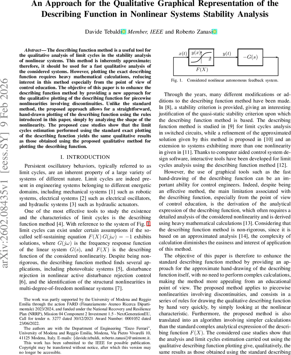
The describing function method is a useful tool for the qualitative analysis of limit cycles in the stability analysis of nonlinear systems. This method is inherently approximate; therefore, it should be used for a fast qualitative analysis of the considered systems. However, plotting the exact describing function requires heavy mathematical calculations, reducing interest in this method especially from the point of view of control education. The objective of this paper is to enhance the describing function method by providing a new approach for the qualitative plotting of the describing function for piecewise nonlinearities involving discontinuities. Unlike the standard method, the proposed approach allows for a straightforward, hand-drawn plotting of the describing function using the rules introduced in this paper, simply by analyzing the shape of the nonlinearity. The proposed case studies show that the limit cycles estimation performed using the standard exact plotting of the describing function yields the same qualitative results as those obtained using the proposed qualitative method for plotting the describing function.

💡 Research Summary

The paper addresses a long‑standing practical obstacle in the use of the Describing Function (DF) method for nonlinear system stability analysis: the difficulty of obtaining the exact DF for piecewise‑linear nonlinearities that contain discontinuities. While the DF method is a powerful tool for quickly estimating the existence and approximate characteristics of limit cycles, its conventional implementation requires evaluating integrals (Eqs. 3‑4) that become cumbersome for multi‑segment nonlinearities. This computational burden limits the method’s appeal, especially in control education where a fast, intuitive approach is preferred.

To overcome this, the authors first revisit two elementary nonlinear blocks that have closed‑form DFs: the dead‑zone (Eq. 5‑6) and the relay with a threshold (Eq. 7‑8). They demonstrate that any piecewise‑linear nonlinearity can be expressed as a linear combination of these two basic blocks (Property 1). By decomposing a given characteristic into segments with slopes (m_i) and possible jumps (Y_j), the overall DF becomes a sum of scaled dead‑zone and relay DFs.

Algorithm 1 implements this decomposition numerically. It takes as input the vectors of break‑points ((x_i, y_i)) and a vector of sinusoid amplitudes (X). For each segment it computes the appropriate (\Phi) (dead‑zone contribution) and (\Psi) (relay contribution) functions and accumulates them to produce a sampled DF (F(X)). The MATLAB code is made publicly available, ensuring reproducibility.

Recognizing that the numerical DF still requires a computer, the authors propose a purely qualitative, hand‑drawn representation. Property 2 and Algorithm 2 define a set of graphical rules that approximate the DF shape using two prototype curves: an exponential‑like rise (\tilde\Phi) (mirroring the dead‑zone DF) and an impulsive‑like pulse (\tilde\Psi) (mirroring the relay DF). The rules are:

1. The qualitative DF (\tilde F(X)) is continuous for (X>0).
2. If the nonlinearity is discontinuous at the origin, (\tilde F(0)=\infty).
3. For amplitudes below the first breakpoint (X_1), (\tilde F) equals the slope of the first linear segment (m_0).
4. As (X\to\infty), (\tilde F) tends to the slope of the last segment (m_r).
5. Within each interval (