$\partial$CBDs: Differentiable Causal Block Diagrams

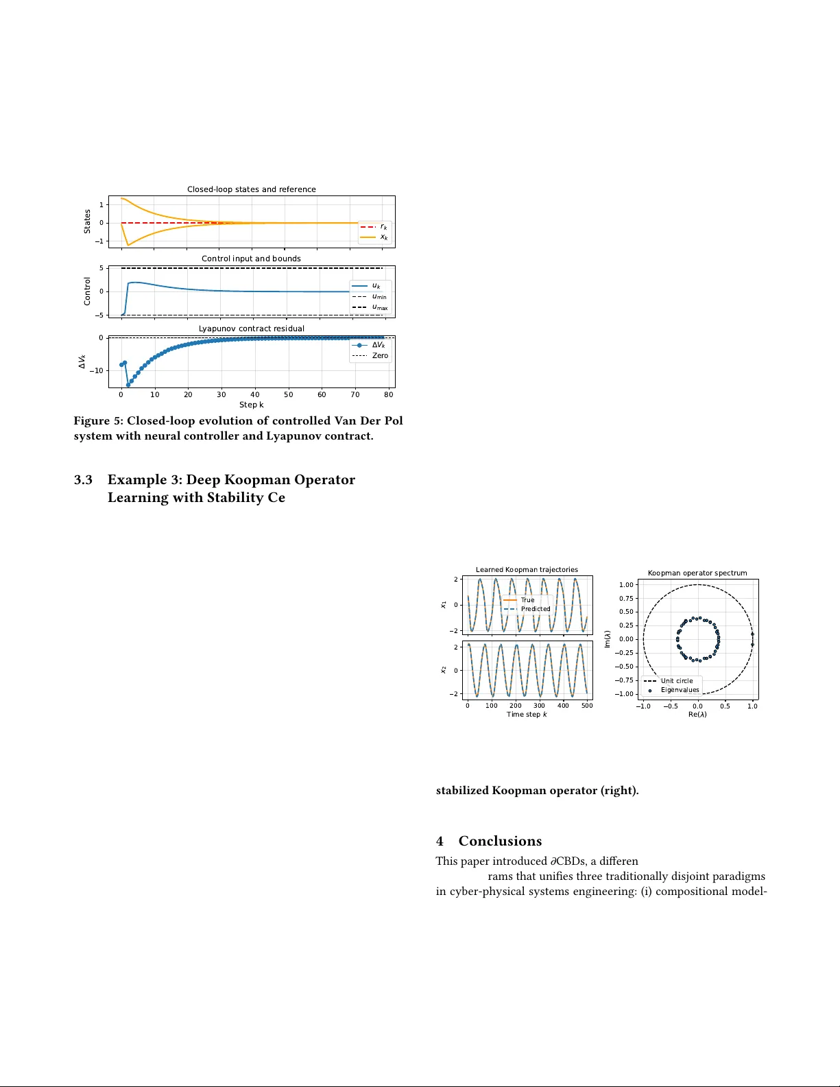
𝜕 CBDs: Dierentiable Causal Block Diagrams Thomas Beckers ∗ V anderbilt University Nashville, USA thomas.beckers@vanderbilt.edu Ján Drgoňa ∗ Johns Hopkins University Maryland, USA jdrgona1@jh.edu Truong X. Nghiem ∗ University of Central Florida Orlando, USA truong.nghiem@ucf.edu Abstract Modern cyber-physical systems (CPS) integrate physics, compu- tation, and learning, demanding modeling frameworks that are simultaneously composable, learnable, and veriable. Y et existing approaches treat these goals in isolation: causal block diagrams (CBDs) support modular system interconnections but lack dieren- tiability for learning; dierentiable programming (DP) enables end- to-end gradient-based optimization but provides limited correctness guarantees; while contract-based verication frameworks remain largely disconnected from data-driven model renement. T o address these limitations, we introduce dierentiable causal block diagrams ( 𝜕 CBDs), a unifying formalism that integrates these three perspec- tives. Our approach (i) retains the compositional structure and execution semantics of CBDs, (ii) incorporates assume–guarantee (A –G) contracts for modular correctness reasoning, and (iii) intro- duces residual-based contracts as dier entiable, trajector y-lev el cer- ticates compatible with automatic dierentiation ( AD), enabling gradient-based optimization and learning. T ogether , these elements enable a scalable, veriable , and trainable modeling pipeline that preserves causality and modularity while supporting data-, physics-, and constraint-informed optimization for CPS. Ke ywords causal block diagrams, assume-guarantee, dierentiable program- ming, physics-informed machine learning A CM Reference Format: Thomas Beckers, Ján Drgoňa, and Truong X. Nghiem. 2018. 𝜕 CBDs: Dier- entiable Causal Block Diagrams. In Proceedings of ACM/IEEE International Conference on Cyber-P hysical Systems (ICCPS) (ICCPS 2026) . A CM, New Y ork, NY, USA, 12 pages. https://doi.org/XXXXXXX.XXXXXXX 1 Introduction Cyber-physical systems increasingly blend model-based design with data-driven components to achieve performance across di- verse operating conditions [42, 27, 4, 10]. As these systems scale in complexity and autonomy , engineers face a three-way tension: com- positionality to manage structural complexity , learnability to adapt models and controllers from data, and veriability to ensure safety ∗ Authors ar e listed in alphabetical order; all authors contributed equally to this work. Permission to make digital or hard copies of all or part of this work for personal or classroom use is granted without fee provided that copies are not made or distributed for prot or commercial advantage and that copies bear this notice and the full citation on the rst page. Copyrights for components of this work owned by others than the author(s) must be honor ed. Abstracting with cr edit is permitted. T o copy otherwise, or republish, to post on servers or to r edistribute to lists, requires prior specic permission and /or a fee. Request permissions from permissions@acm.org. ICCPS 2026, Saint Malo, France © 2018 Copyright held by the owner/author(s). Publication rights licensed to A CM. ACM ISBN 978-1-4503-XXXX -X/2018/06 https://doi.org/XXXXXXX.XXXXXXX and correctness [48]. T oday’s methodologies typically address one or two of these requir ements, but rarely unify all three in a sin- gle, tractable workow . Causal block diagrams (CBDs) remain the lingua franca of CPS design, see [28], due to their clear e xecution semantics and support for modular composition, yet they ar e not natively dierentiable and thus only weakly connected to modern optimization and learning pipelines. Dierentiable pr ogramming (DP) framew orks pro vide end-to-end gradients and sensitivity anal- ysis, but operate over computational graphs whose semantics ar e geared toward numerical execution rather than correctness and compositional reasoning [31]. Modern DP systems typically rely on automatic dierentiation (AD) as their computational backbone, en- abling ecient gradient propagation but oering limited structure for specifying or verifying formal contracts. Contract-based veri- cation, especially via assume-guarantee spe cications, provides scalable certication [12], but is typically decoupled from learning, making it hard to enforce safety and performance constraints dur- ing data-driven optimization. This disconnect forces practitioners to choose between structured, certiable models that are dicult to optimize and learning tools that lack robust assurances. This pap er introduces dierentiable Causal Block Diagrams ( 𝜕 CBDs), a modeling and optimization framework that integrates CBD compositionality , assume-guarantee contract semantics, and dierentiable programming into a single pipeline. In 𝜕 CBDs, each block is equipped with explicit interfaces and time semantics, an execution map that may be continuous, discrete, or hybrid, and a set of dierentiable contract residuals that formalize assump- tions and guarante es. These residuals can quantify property sat- isfaction—such as passivity , gain bounds, and Lyapunov certi- cates—and can be composed across interconnections while pre- serving execution semantics. Crucially , 𝜕 CBD compositions yield automatic-dierentiation-executable graphs over nite horizons by rate lifting and loop unrolling, enabling gradients to propagate through physics-based models (e.g., ODE/D AE solvers, xed-p oint and optimization layers) and data-driven components (e.g., neural networks) in a principled manner . Contracts thus become dier- entiable certicates that can be enforced or regularized during training, which allo ws learning to be guided by physics, safety , and performance constraints rather than solely by empirical loss. Related works. A utomatic dierentiation (AD) has become the computational backbone of modern machine learning and scientic computing, enabling ecient, machine-precision gradients through arbitrarily complex programs. In machine learning, rev erse-mode AD underpins deep learning frameworks such as T ensorFlow , Py- T orch, and JAX, supporting large-scale optimization of neural archi- tectures [1, 37, 16]. In scientic computing and optimal contr ol, AD extends to dierential e quations, providing sensitivities through numerical solvers [6, 29, 30, 18]. These advances hav e established AD as the key enabler of dierentiable programming , a paradigm ICCPS 2026, May 11-14, 2026, Saint Malo, France Thomas Beckers, Ján Drgoňa, and Truong X. Nghiem that unies simulation, learning, and optimization within a single computational graph [31, 9, 47, 15]. Building on this foundation, the proposed 𝜕 CBD framework embeds AD semantics directly into the compositional structure of CBDs, enabling scalable, v eriable, and physically grounded learning in cyber-physical systems. Contributions. First, we propose a dierentiable extension of causal block diagrams that preserves compositional structure and execution semantics while enabling end-to-end gradient-based op- timization. Second, we embed assume-guarantee contracts as dier- entiable residuals within the modeling pipeline, turning modular specications into optimization-aware certicates that guide and constrain learning. Third, we de velop a reduction from 𝜕 CBDs to AD-executable graphs with well-dened sensitivity propagation across heterogeneous components, providing a foundation for scal- able training and verication of CPS. Collectively , these elements establish a practical and principled basis for designing systems that are simultaneously composable, learnable, and veriable . 2 Methodology W e introduce dierentiable Causal Blo ck Diagrams ( 𝜕 CBDs), a for- malism that unies (i) the compositional modeling of CBDs, (ii) assume-guarantee ( A –G) contracts for modular correctness, and (iii) dierentiable programming (DP) for end-to-end learning. By combining the structural clarity of CBDs, the compositional veri- cation power of A –G contracts, and the scalability of automatic dierentiation (AD) frameworks, our approach enables scalable, veriable, and composable modeling, learning, and optimization of complex cyber-physical systems. In the proposed 𝜕 CBD framework, each block is endowed with a dierentiable contract encoding its physical, safety , or operational properties. CBD compositions (serial, parallel, or feedback) preserve these properties through contract composition and are translated to AD-executable directe d acyclic graphs (D AGs). The resulting system behaves both as a causal diagram (for simulation and mo d- ular reasoning) and as a dier entiable program (for learning and optimization). A –G contracts are embe dded as smooth penalty or certicate functions within the computational graph, enabling for- mal correctness reasoning to coexist with gradient-based training. Formally , the 𝜕 CBD framework consists of ve layers of abstraction: (1) Structural layer: denes the block with contract as a fun- damental unit in the causal block diagrams (Sec. 2.1); (2) Semantic layer: denes the composition rules and causal execution semantics for blocks (Sec. 2.2); (3) Contract layer: assigns assume-guarante e specications to blocks, ensuring compositional correctness (Sec. 2.3); (4) Dierentiable layer: exposes derivatives of the causal blo ck diagrams via automatic dierentiation (Sec. 2.4). (5) Optimization layer: enables veriable gradient-based learn- ing and optimization for causal block diagrams (Sec. 2.5). T ogether , these layers yield a unied modeling and learning pipeline that preserves causality and compositional structure , ex- poses local gradients through AD-compatible primitives, and sup- ports system-level verication via dier entiable contracts at scale. This integration forms the methodological core of 𝜕 CBDs. 2.1 Causal Block Diagrams with Contracts The causal block diagram (CBD) is a widely adopted modeling for- malism for practical model-based design of CPS [28]. Perhaps the most prominent CBD implementation is Simulink [20], with recent extensions for contract-based semantics and renement [43, 52]. Similarly , Ptolemy II adopts the CBD as its core modeling para- digm, pr oviding a exible framework for composing heterogeneous models of computation within a unied block-based architecture [38]. Our framework adopts the core CBD formalism commonly used in these implementations and the literature, described below . The assume-guarantee (A –G) contract extension to CBD will be presented in Section 2.3. Notations. An indexed lowercase letter , like 𝑣 𝑖 , denotes a variable, an uppercase letter , like 𝑉 , is a set of variables 𝑣 𝑖 , a bold upp ercase letter , like 𝑽 , is the vector concatenation of variables in 𝑉 , and a calligraphic letter , like V , is the value space of 𝑽 . Signals. W e rst dene signals , which are functions from time to values, that represent time-varying variables in a system. The time domain is represented by non-negative r eal numbers, denoted by R + . A signal can either be continuous-time or discrete-time . Denition 2.1 (Signal). A continuous-time signal 𝑠 is a function from R + to 𝑆 , where 𝑆 is the non-empty set of values of the signal. A discrete-time signal 𝑠 is a piece-wise constant continuous-time signal whose value only changes at discr ete time instants 𝑘 𝜏 , where the natural numb er 𝑘 ∈ N is the time step and the p ositive real constant 𝜏 is the p eriod, i.e., ∀ 𝑡 ∈ [ 𝑘 𝜏 , ( 𝑘 + 1 ) 𝜏 ) , 𝑠 ( 𝑡 ) = 𝑠 ( 𝑘𝜏 ) . In the above denition, the value set 𝑆 can be any non-empty set, including nite sets of discrete values such as the Boolean set. In practice, howev er , 𝑆 is often the real number set R . In this work, for simplicity , we assume that 𝑆 ≡ R . Blocks. In a CBD, a block represents a component that typically transforms some input signals to some output signals with well- dened behaviors. In our framework, each block can b e associated with an assume-guarantee contract , which species the behaviors of the block under given conditions. Contracts ar e a key element in our framework for verication and for learning, specifying sys- tem properties such as safety requirements and physical priors that can b e integrated into learning. A block can be continuous- time, discrete-time, or hybrid ( where b oth continuous-time and discrete-time behaviors exist), and can have multiple associated sampling periods. W e adopt the following formalization of a block with contract , illustrated in Fig. 1a. Denition 2.2 (Blo ck with Contract). A block is a tuple B = ( 𝑈 , 𝑋 , 𝑌 , 𝑇 , 𝐹 , 𝑔, Init , C ) , • 𝑈 = { 𝑢 1 , . . . , 𝑢 𝑛 } is the set of input variables , each denot- ing a signal that is consumed by the blo ck. 𝑼 is the vector concatenation of all input variables and U is its value space. • 𝑋 = { 𝑥 1 , . . . , 𝑥 𝑝 } is the set of internal state variables , each denoting a signal that is internal to t he block. 𝑿 is the vector concatenation of all state variables and X is its value space. • 𝑌 = { 𝑦 1 , . . . , 𝑦 𝑚 } is the set of output variables , each denot- ing a signal that is generated by the blo ck. 𝒀 is the vector concatenation of all output variables and Y is its value space. 𝜕 CBDs: Dierentiable Causal Block Diagrams ICCPS 2026, May 11-14, 2026, Saint Malo, France • 𝑇 is the time semantics of the block, which is a set of unique sampling periods 𝑇 = { 𝜏 1 , . . . , 𝜏 𝑞 } , 𝜏 𝑖 ∈ R + , with the conven- tion that a zero sampling period means continuous-time. 𝑇 must contain at least one element. • 𝐹 = { 𝑓 ( 𝜏 ) } 𝜏 ∈ 𝑇 is the set of state transition functions 𝑓 ( 𝜏 ) corresponding to the sampling p eriods 𝜏 in 𝑇 . Each 𝑓 ( 𝜏 ) only updates a non-empty subset 𝑋 ( 𝜏 ) ⊆ 𝑋 of the state variables, and the set of 𝑋 ( 𝜏 ) is a partition of 𝑋 , i.e., ∪ 𝜏 ∈ 𝑇 𝑋 ( 𝜏 ) = 𝑋 and for any 𝜏 , 𝜏 ′ ∈ 𝑇 , 𝑋 ( 𝜏 ) ∩ 𝑋 ( 𝜏 ′ ) = ∅ . The semantic of 𝑓 ( 𝜏 ) depends on its time semantic: – If 𝜏 = 0 : all state signals in 𝑋 ( 0 ) are continuous-time and have continuous values, and 𝑓 ( 0 ) denes a dierential equation: ¤ 𝑿 ( 0 ) ( 𝑡 ) = 𝑓 ( 0 ) ( 𝑿 ( 𝑡 ) , 𝑼 ( 𝑡 ) ) , that is well-dened with unique solution 𝑿 ( 0 ) ( 𝑡 ) for any initial condition. – If 𝜏 > 0 : all state signals in 𝑋 ( 𝜏 ) are discrete-time and can be either continuous or discrete. Their values are updated at each discrete time instant 𝑘 𝜏 by the dierence equation: 𝑿 ( 𝜏 ) ( ( 𝑘 + 1 ) 𝜏 ) = 𝑓 ( 𝜏 ) ( 𝑿 ( 𝑘𝜏 ) , 𝑼 ( 𝑘 𝜏 ) ) . • 𝑔 is the output function that calculates the outputs 𝑌 from the current states and inputs: 𝒀 ( 𝑡 ) = 𝑔 ( 𝑿 ( 𝑡 ) , 𝑼 ( 𝑡 ) ) . It can represent an explicit equation from 𝑿 and 𝑼 to 𝒀 or an implicit equation of the form 𝒀 ( 𝑡 ) = ℎ ( 𝒀 ( 𝑡 ) , 𝑿 ( 𝑡 ) , 𝑼 ( 𝑡 ) ) , solved by a xed-point solver . • Init is the initial condition of the states 𝑋 , i.e., 𝑿 ( 0 ) = Init . • C is a set of contracts satised by the block (see Sec. 2.3). Assumption 1 (Block). A blo ck must satisfy the following: • It has at least one input or output, i.e., the sets 𝑈 , 𝑋 , and 𝑌 can be empty but 𝑈 and 𝑌 cannot be both empty . • Its dynamics, specie d by the state transition functions 𝑓 ( 𝜏 ) and the output functions 𝑔 𝜏 , are causal. • Its dynamics are driv en by time, not by ev ents. Remark 1. W e make the following remarks. • If 𝑈 is empty then the block is a source block that generates signals. If 𝑌 is empty then it is a sink block that only consumes signals. If 𝑋 is empty then the block is stateless or static ; otherwise, the block is stateful or dynamic . • A block may be hybrid, having both a continuous-time se- mantic ( 𝜏 = 0 ) and discrete-time semantics ( 𝜏 > 0 ). • For the r emainder of this paper , w e will focus on continuous- valued states 𝑋 . Event-driven dynamics with discr ete state variables will be investigated in future research. 2.2 Execution and Composition of CBDs Given a block B and its input signals 𝑼 ( 𝑡 ) = { 𝑢 1 ( 𝑡 ) , . . . , 𝑢 𝑛 ( 𝑡 ) } , the block can be executed to generate state signals 𝑿 ( 𝑡 ) = { 𝑥 1 ( 𝑡 ) , . . . , 𝑥 𝑝 ( 𝑡 ) } and output signals 𝒀 ( 𝑡 ) = { 𝑦 1 ( 𝑡 ) , . . . , 𝑦 𝑚 ( 𝑡 ) } , for 0 ≤ 𝑡 ≤ 𝑡 𝑓 where 𝑡 𝑓 is the nal time, by solving the causal dierential and dierence equations resulting from 𝐹 . A brief description of the block execution algorithm is given below . (1) Based on the discrete sampling periods in 𝑇 , a sequence of time instants 0 = 𝑡 0 , 𝑡 1 , . . . , 𝑡 𝑁 = 𝑡 𝑓 is determined, where for each 𝑡 𝑖 with 0 < 𝑖 < 𝑁 , there exists 𝜏 ∈ 𝑇 such that 𝑡 𝑖 = 𝑘 𝜏 for some 𝑘 ∈ N . (2) Initial states and outputs are set: 𝑿 ( 0 ) = Init and 𝒀 ( 0 ) = 𝑔 ( 𝑿 ( 0 ) , 𝑼 ( 0 ) ) . U Y State X state transitions F = { f ( τ ) } τ ∈ T X (0) = Init g Block B Contracts C (a) The components and semantics of a block . U 1 B 1 U 2 B 2 Y 1 Y 2 B (b) Parallel composi- tion. U 1 B 1 U − 2 B 2 Y σ 1 Y 1 Y 2 B (c) Serial composition. B U − Y σ Y B (d) Fee dback composition. Figure 1: Illustrations of blocks and their compositions. (3) For each interval ( 𝑡 𝑖 , 𝑡 𝑖 + 1 ] , the corresponding dierential equation and dierence equations ar e solved from the initial condition 𝑿 ( 𝑡 𝑖 ) to obtain the state values in the interval. Then, the output signals 𝑌 are calculated by 𝑔 . If the signals 𝑿 ( 𝑡 ) and 𝒀 ( 𝑡 ) are generated by the execution se- mantics of B from the input signals 𝑼 ( 𝑡 ) , we write ( 𝑿 ( 𝑡 ) , 𝒀 ( 𝑡 ) ) ∈ Exec ( B , 𝑼 ( 𝑡 ) ) . As a consequence, each block denes an input– output map from the input signals 𝑼 ( 𝑡 ) to the output signals 𝒀 ( 𝑡 ) , denoted by 𝒀 = B ( 𝑼 ) using the same block notation. Compositions of blo cks. A CBD consists of blocks that are in- terconnected. A CBD can be “attened” to an equivalent block by composing its blo cks and their connections in a directe d acyclic graph (DA G). The remainder of this section formalizes a unilateral connection between two blocks and the fundamental composition rules of blocks. Denition 2.3 (Unilateral Connection). Given two blocks B 𝑖 = ( 𝑈 𝑖 , 𝑋 𝑖 , 𝑌 𝑖 , 𝑇 𝑖 , 𝐹 𝑖 , 𝑔 𝑖 , Init 𝑖 , C 𝑖 ) , 𝑖 = 1 , 2 , a unilateral connection 𝜎 1 , 2 from B 1 to B 2 is a relation 𝜎 1 , 2 = { ( 𝑦 1 , 𝑖 , 𝑢 2 , 𝑗 ) | 𝑦 1 , 𝑖 ∈ 𝑌 1 , 𝑢 2 , 𝑗 ∈ 𝑈 2 } satisfying: (1) The output and input in each pair ( 𝑦 1 , 𝑖 , 𝑢 2 , 𝑗 ) are compatible in terms of types and dimensions; (2) Only one output can be connected to an input; (3) 𝑢 2 , 𝑗 ( 𝑡 ) = 𝑦 1 , 𝑖 ( 𝑡 ) for all 𝑡 ∈ R + . The set of outputs and the set of inputs in the connection 𝜎 1 , 2 are denoted by 𝜎 out 1 , 2 ⊆ 𝑌 1 and 𝜎 in 1 , 2 ⊆ 𝑈 2 , respectively . A CBD is thus a composition of blocks and their connections. Denition 2.4 (Causal Block Diagram (CBD)). A CBD is a tuple D = ( B , Σ ) of blocks B = { B 𝑖 } 𝑖 and a set of unilateral connections between these blocks Σ = { 𝜎 𝑖 , 𝑗 | B 𝑖 ∈ B , B 𝑗 ∈ B } . The connections must satisfy that no more than one output can be connecte d to an input, but an output can be connected to more than one input. W e now dene the semantics of three elementary composition operators that can be use d to compose a more complex CBDs. The following notation will be required: if 𝑓 : 𝑋 ↦→ 𝑌 is a function with a vector of output variables 𝑌 and 𝑌 ′ ⊆ 𝑌 , then 𝑓 | 𝑌 ′ denotes the ICCPS 2026, May 11-14, 2026, Saint Malo, France Thomas Beckers, Ján Drgoňa, and Truong X. Nghiem function 𝑓 restricted to the subset 𝑌 ′ of outputs, i.e., 𝑓 | 𝑌 ′ : = 𝜋 𝑌 ′ ◦ 𝑓 where 𝜋 𝑌 ′ is the projection operator from 𝑌 to 𝑌 ′ . A parallel composition of two blo cks, illustrated in Fig. 1b, simply combines the two blocks into a single block. Denition 2.5 (Parallel Composition). Given tw o blocks B 𝑖 = ( 𝑈 𝑖 , 𝑋 𝑖 , 𝑌 𝑖 , 𝑇 𝑖 , 𝐹 𝑖 , 𝑔 𝑖 , Init 𝑖 , C 𝑖 ) , 𝑖 = 1 , 2 . A parallel comp osition B 1 ∥ B 2 is a blo ck B = ( 𝑈 , 𝑋 , 𝑌 , 𝑇 , 𝐹 , 𝑔, Init , C ) with 𝑈 = 𝑈 1 ∪ 𝑈 2 , 𝑋 = 𝑋 1 ∪ 𝑋 2 , 𝑌 = 𝑌 1 ∪ 𝑌 2 , 𝑇 = 𝑇 1 ∪ 𝑇 2 , 𝐹 = 𝐹 1 ∪ 𝐹 2 , 𝑔 ( 𝑿 , 𝑼 ) = ( 𝑔 1 ( 𝑿 1 , 𝑼 1 ) , 𝑔 2 ( 𝑿 2 , 𝑼 2 ) ) , Init = ( Init 1 , Init 2 ) , and the composed con- tract C to be presented in Section 2.3. A serial composition of two blocks connects some outputs of one block to some inputs of the other block, as illustrated in Fig. 1c. Denition 2.6 (Serial Composition). Given two blocks B 𝑖 = ( 𝑈 𝑖 , 𝑋 𝑖 , 𝑌 𝑖 , 𝑇 𝑖 , 𝐹 𝑖 , 𝑔 𝑖 , Init 𝑖 , C 𝑖 ) , 𝑖 = 1 , 2 , and a conne ction 𝜎 1 , 2 from B 1 to B 2 . Let 𝑈 − 2 = 𝑈 2 \ 𝜎 in 1 , 2 denote the inputs of B 2 not conne cted by the conne ction 𝜎 1 , 2 , and let 𝑌 𝜎 1 = 𝜎 out 1 , 2 denote the outputs of B 1 connected to B 2 . A serial composition B 1 ; B 2 is a block B = ( 𝑈 , 𝑋 , 𝑌 , 𝑇 , 𝐹 , 𝑔, Init , C ) with • 𝑈 = 𝑈 1 ∪ 𝑈 − 2 , 𝑋 = 𝑋 1 ∪ 𝑋 2 , 𝑌 = 𝑌 1 ∪ 𝑌 2 , 𝑇 = 𝑇 1 ∪ 𝑇 2 , • 𝐹 = 𝐹 1 ∪ 𝐹 𝜎 2 , where 𝐹 𝜎 2 consists of the same state transi- tion functions in 𝐹 2 restricted to the connected inputs deter- mined by 𝜎 1 , 2 . Specically , each 𝑓 ( 𝜏 ) 2 ( 𝑿 2 , 𝑼 2 ) in 𝐹 2 becomes 𝑓 ( 𝜏 ) 2 ( 𝑿 2 , ( 𝑼 − 2 , 𝑔 1 | 𝑌 𝜎 1 ( 𝑿 1 , 𝑼 1 ) ) ) = 𝑓 ( 𝜏 ) 2 ( 𝑿 , 𝑼 ) in 𝐹 𝜎 2 . • 𝑔 ( 𝑿 , 𝑼 ) = ( 𝑔 1 ( 𝑿 1 , 𝑼 1 ) , 𝑔 2 ( 𝑿 2 , ( 𝑼 − 2 , 𝑔 1 | 𝑌 𝜎 1 ( 𝑿 1 , 𝑼 1 ) ) ) ) reects the connection from B 1 to B 2 . It can also be represented as two steps: 𝒀 1 = 𝑔 1 ( 𝑿 1 , 𝑼 1 ) and 𝒀 2 = 𝑔 2 ( 𝑿 2 , ( 𝑼 − 2 , 𝜋 𝑌 𝜎 1 ( 𝒀 1 ) ) ) . • Init = ( Init 1 , Init 2 ) • C is the compose d contract, to be presented in Section 2.3. An important and commonly used composition in CBDs is the feedback composition , which fee ds some outputs of a block B back into some of its own inputs by a directed cycle, as illustrated in Fig. 1d. A challenge of the fee dback composition is the algebraic loop feedback . W e rst describe the concept of a direct feedthrough . If the output function 𝑔 of a block B is such that an input 𝑢 𝑖 is directly fe d through 𝑔 to an output 𝑦 𝑗 , i.e., the value of 𝑢 𝑖 ( 𝑡 ) directly aect the value of 𝑦 𝑗 ( 𝑡 ) , then B has a direct feedthrough from 𝑢 𝑖 to 𝑦 𝑗 . An algebraic loop occurs when the conne ctions b etween the outputs and inputs in a feedback composition form a closed cycle of direct feedthroughs, i.e., 𝑢 𝑖 is directly fed thr ough to 𝑦 𝑗 and 𝑦 𝑗 is connecte d to 𝑢 𝑖 . In other words, an output of the blo ck is driven by itself in the same time step. Although an algebraic loop can be expressed as an algebraic equation, solved in the CBD execution, there are inherent diculties in handling it in this way . An alternative technique for handling an algebraic lo op is to break it by articially inserting a stateful blo ck, such as a unit-time delay or an integrator , into the loop. While this might slightly alter the semantics of the original CBD , it is straightfor ward and is ther efore often employed in practice, e.g., in Simulink. For simplicity , we will assume that all feedback compositions are algebraic loop-free. Assumption 2. There are no algebraic loops in the CBD. Removing this assumption by e xplicitly handling algebraic loops will be investigated in future research. B C r y Controller Plant u B P + − B Σ r  ( B Σ ; B C ; B P ) ( B Σ ; B C ; B P ) y u r y u Figure 2: A standard fe edback control loop (top) can be at- tened into an e quivalent blo ck (bottom right) using the serial composition and feedback composition rules. Denition 2.7 (Fe edback Composition). Given a block B = ( 𝑈 , 𝑋 , 𝑌 , 𝑇 , 𝐹 , 𝑔, Init , C ) and a connection 𝜎  from B to itself. The com- position is assumed to be algebraic loop-free. Let 𝑈 − = 𝑈 \ 𝜎 in  denote the inputs of B not connected by the conne ction 𝜎  and let 𝑌 𝜎 = 𝜎 out  denote the outputs of B connected by 𝜎  . The algebraic loop-free fee dback composition ⟳ B is a blo ck B  = ( 𝑈  , 𝑋  , 𝑌  , 𝑇  , 𝐹  , 𝑔  , Init  , C  ) with • 𝑈  = 𝑈 − , 𝑋  = 𝑋 , 𝑌  = 𝑌 , and 𝑇  = 𝑇 , • 𝐹  = 𝐹 𝜎 consists of the same state transition functions in 𝐹 restricted to the connected inputs determine d by 𝜎 𝑖 , 𝑗 . These functions are well-dened if no algebraic loops exist. • 𝑔  ( 𝑿  , 𝑼  ) = 𝑔 ( 𝑿  , ( 𝑼  , 𝑔 | 𝑌 𝜎 ( 𝑿  , 𝑼  ) ) ) is well-dened without algebraic loops. With algebraic loops, 𝑔  becomes an implicit equation, which is allowed in Denition 2.2 and can be solved by a xed-p oint solver under mild conditions. • Init  = Init • C is the compose d contract, to be presented in Section 2.3. The above compositions have several useful pr operties. Lemma 2.8. Given blocks B 1 , B 2 , and B 3 , and admissible conne c- tions between them, the following properties hold. (1) ( B 1 ; B 2 ) ; B 3 = B 1 ; ( B 2 ; B 3 ) (2) B 1 ∥ B 2 = B 2 ∥ B 1 (3) ( B 1 ∥ B 2 ) ∥ B 3 = B 1 ∥ ( B 2 ∥ B 3 ) . These properties follow directly from the associativity and com- mutativity of signal concatenation and substitution in the CBD exe- cution semantics and are standard in CBD formalisms [28, 52].Using these fundamental compositions and their pr operties, any algebraic loop-free CBD D = ( B , Σ ) can be converted, or attened , into an equivalent blo ck B with the same execution semantics as the original CBD. Fig. 2 demonstrates how a standard feedback control CBD is attened into an e quivalent block using the fundamental composition rules. W e rst apply the serial composition rule on the feedfor ward path, which consists of the sum blo ck B Σ , the con- troller block B 𝐶 , and the plant block B 𝑃 , to obtain the composed block ( B Σ ; B 𝐶 ; B 𝑃 ) . W e then apply the feedback comp osition rule on this composed block to atten the original CBD into the block ⟳ ( B Σ ; B 𝐶 ; B 𝑃 ) , which has the reference signal 𝑟 as input, and the control signal 𝑢 and plant output signal 𝑦 as outputs. 𝜕 CBDs: Dierentiable Causal Block Diagrams ICCPS 2026, May 11-14, 2026, Saint Malo, France Furthermore, any subset of blocks of a CBD and their associated connections, which ar e also a CBD , can be replaced equivalently by their attened block, called a subsystem . A subsystem can contain other subsystems. Consequently , this allows any CBD to b e broken into nested subsystems. This also allows a subsystem, represented by its attened block, to be replaced by an appr oximate block, such as a machine learning based model. 2.3 Contracts for CBDs CBDs support modular system construction, but reasoning about the correctness of interconnected blo cks requires explicit specica- tion of contractual guarantees. In this section, we introduce two complementary notions of contracts for CBDs. Assume–guarantee (A –G) contracts provide normative, system-wide specications for compositional correctness reasoning, while residual-based con- tracts provide dierentiable, quantitative certicates for realized executions and are used primarily for optimization and learning. Assume-Guarantee (A –G) Contracts for CBDs. A –G contracts provide a formal framework for reasoning about system correctness through compositional specication and verication [12], and have been successfully integrate d into frameworks such as interface au- tomata [19] and dynamical systems [41]. Building on these ideas, we extend the CBD formalism with A –G contract semantics, allowing for contract-based reasoning within block-structured models. Denition 2.9 (Assume–Guarantee Contract for a Block). An assume– guarantee (A –G) contract for a block B is a pair C AG = ( A , G ) , where A ⊆ U denotes the set of admissible input b ehaviors (as- sumptions), and G ⊆ U × Y denotes the set of guaranteed input– output behaviors. The block B is said to satisfy its contract if ∀ 𝑈 ∈ A : ( 𝑈 , B ( 𝑈 ) ) ∈ G . The composition of A –G contracts mirrors the structural com- position of blocks and is formally dened by projecting and e xis- tentially quantifying internal signals while enforcing compatibility conditions between assumptions and guarantees. For a set S ⊆ U × Y , let 𝜋 𝑈 ( S ) and 𝜋 𝑌 ( S ) denote its projections onto inputs and outputs, respectively . For serial connections 𝜎 1 , 2 , let 𝑈 − 2 = 𝑈 2 \ 𝜎 in 1 , 2 and 𝑌 𝜎 1 = 𝜎 out 1 , 2 as in Denition 2.6, and let 𝜎 1 , 2 ( 𝑌 𝜎 1 ) denote the mapping from signals 𝑌 𝜎 1 to connected signals 𝜎 in 1 , 2 . Denition 2.10 (A –G compatibility for a serial connection). Let C AG 1 = ( A 1 , G 1 ) and C AG 2 = ( A 2 , G 2 ) be A–G contracts for B 1 and B 2 . The serial connection 𝜎 1 , 2 is compatible if every upstream be- havior consistent with C AG 1 supplies a connected signal admissible to B 2 , i.e., 𝜎 1 , 2  𝜋 𝑌 𝜎 1 ( { ( 𝑈 1 , 𝑌 1 ) ∈ G 1 | 𝑈 1 ∈ A 1 } )  ⊆ 𝜋 𝜎 in 1 , 2 ( A 2 ) . Denition 2.11 (A –G contract composition). Let C AG 𝑖 = ( A 𝑖 , G 𝑖 ) be A–G contracts for blocks B 𝑖 . Parallel: The parallel composition B 1 ∥ B 2 has contract C AG ∥ = ( A 1 × A 2 , G 1 × G 2 ) , where ( A 1 × A 2 ) ⊆ ( U 1 × U 2 ) and ( G 1 × G 2 ) ⊆ ( U 1 × U 2 ) × (Y 1 × Y 2 ) . Serial: A ssume 𝜎 1 , 2 is compatible in the sense of Denition 2.10. The serial composition B 1 ; B 2 has contract C AG ; = ( A ; , G ; ) , where A ; ⊆ U 1 × U − 2 consists of external inputs for which the inter- connection is admissible, and G ; ⊆ ( U 1 ×U − 2 ) × ( Y 1 ×Y 2 ) is the set of external input/output behaviors obtained by existentially quantify- ing internal connection signals. Concretely , ( 𝑈 1 , 𝑈 − 2 , 𝑌 1 , 𝑌 2 ) ∈ G ; if there exists a connecte d signal 𝑣 ∈ 𝜋 𝜎 in 1 , 2 ( A 2 ) such that ( 𝑈 1 , 𝑌 1 ) ∈ G 1 and ( ( 𝑈 − 2 , 𝑣 ) , 𝑌 2 ) ∈ G 2 , with 𝑣 identied with 𝜋 𝑌 𝜎 1 ( 𝑌 1 ) . Feedback: Assume the feedback interconnection 𝜎  is well-posed and compatible (analogous to serial compatibility). Then, feedback contracts are handled by unrolling feedback compositions into equivalent serial compositions, following the feedback execution semantics of CBDs, so that contract composition reduces to repeated application of the serial composition rule. This construction is equivalent to existentially quantifying internal feedback signals and projecting onto the remaining external variables. Denition 2.12 (System-level A –G satisfaction). A CBD D = ( B , Σ ) satises its A –G contracts if each block B 𝑖 satises C AG 𝑖 = ( A 𝑖 , G 𝑖 ) under universal semantics and all interconnections in Σ are compatible (i.e., guarantees imply downstream assumptions under the appropriate projections). Residual-based Contracts for CBDs. T o enable veriable opti- mization and learning, we introduce residual-based contracts as quantitative certicates evaluated along realized executions. Denition 2.13 (Residual-Based Contract for a Block). A residual- based contract for a block B is dened by a mapping C res : X × U × Y × R 𝑛 𝜃 → R 𝑚 , where 𝜃 ∈ R 𝑛 𝜃 parameterizes the contract. A realized execution ( 𝑋 , 𝑈 , 𝑌 ) is said to satisfy the residual-based contract if C res ( 𝑋 , 𝑈 , 𝑌 ; 𝜃 ) ≤ 0 holds element-wise. Residual satisfaction constitutes a sucient certicate that the realized input–output behavior ( 𝑈 , 𝑌 ) satises the corresponding guarantee for the given execution. Residual-based contracts are composed at the structural level according to the CBD execution semantics, by aggregating lo cal residuals and substituting connected outputs into inputs. Denition 2.14 (Residual contract composition). Consider residual- based contracts C res 𝑖 ( 𝑋 𝑖 , 𝑈 𝑖 , 𝑌 𝑖 ; 𝜃 𝑖 ) ≤ 0 for blocks B 𝑖 . Parallel: The parallel composition B 1 ∥ B 2 has residual contract given by concatenation C res ∥ ( 𝑋 , 𝑈 , 𝑌 ; 𝜃 ) =  C res 1 ( 𝑋 1 , 𝑈 1 , 𝑌 1 ; 𝜃 1 ) C res 2 ( 𝑋 2 , 𝑈 2 , 𝑌 2 ; 𝜃 2 )  ≤ 0 , with 𝑋 = ( 𝑋 1 , 𝑋 2 ) , 𝑈 = ( 𝑈 1 , 𝑈 2 ) , 𝑌 = ( 𝑌 1 , 𝑌 2 ) , and 𝜃 = ( 𝜃 1 , 𝜃 2 ) . Serial: For a serial interconnection 𝜎 1 , 2 , dene 𝑈 − 2 = 𝑈 2 \ 𝜎 in 1 , 2 and 𝑌 𝜎 1 = 𝜎 out 1 , 2 . The serial composition B 1 ; B 2 has residual contract C res ; ( 𝑋 , 𝑈 , 𝑌 ; 𝜃 ) =  C res 1 ( 𝑋 1 , 𝑈 1 , 𝑌 1 ; 𝜃 1 ) C res 2  𝑋 2 , ( 𝑈 − 2 , 𝑌 𝜎 1 ) , 𝑌 2 ; 𝜃 2   ≤ 0 . ICCPS 2026, May 11-14, 2026, Saint Malo, France Thomas Beckers, Ján Drgoňa, and Truong X. Nghiem Feedback: For a fe edback interconnection 𝜎  , let 𝑈 − = 𝑈 \ 𝜎 in  and 𝑌 𝜎 = 𝜎 out  . The feedback composition ⟳ B has residual contract C res ⟳ ( 𝑋 , 𝑈 − , 𝑌 ; 𝜃 ) = C res  𝑋 , ( 𝑈 − , 𝑌 𝜎 ) , 𝑌 ; 𝜃  ≤ 0 , where 𝑌 𝜎 denotes the feedback outputs substituted into the corre- sponding feedback inputs. Denition 2.15 (System-level residual satisfaction). A CBD D = ( B , Σ ) satises its residual-based contracts for a realized execu- tion if, for each block B 𝑖 , one has C res 𝑖 ( 𝑋 𝑖 , 𝑈 𝑖 , 𝑌 𝑖 ; 𝜃 𝑖 ) ≤ 0 , and all interconnections respect admissible input domains. Remark 2 (Residual contracts as exact A –G contracts). In special cases, a residual-based contract admits an exact interpretation as an A –G contract when it encodes a ne cessary and sucient condi- tion for the guarantee set G and is enforced by construction for all admissible executions. In this setting, the residual dep ends only on parameters (or structural properties) of CBD and not on specic trajectories, yielding a univ ersally quantied guarantee. Otherwise, residual-based contracts are trajectory-dependent and provide suf- cient certicates only for the realized execution. W e demonstrate representative structural property cases in Examples 1 and 3 in Sec- tion 3. Characterizing and e xploiting this equivalence more broadly is a direction for future work. 2.4 Dierentiable Causal Blo ck Diagrams A utomatic dierentiation ( AD) relies on Jacobian–vector products ( JVPs) and vector–Jacobian products (VJPs). For a dierentiable map 𝐹 : R 𝑛 → R 𝑚 with Jacobian 𝐽 𝐹 = 𝜕𝐹 𝜕𝑥 , these are dened as JVP ( 𝑣 ) = 𝐽 𝐹 𝑣 , VJP ( ¯ 𝑣 ) = 𝐽 ⊤ 𝐹 ¯ 𝑣 . (1) Here, 𝑣 denotes a tangent (perturbation) direction in the input space, and ¯ 𝑣 an adjoint (co-vector) in the output space. The JVP computes directional derivatives in the forward mode (sensitivity propaga- tion), while the VJP computes adjoint sensitivities in the reverse mode (gradient backpropagation). W e assume throughout that all maps are dened on op en sets of appropriate Euclidean spaces; statements “a.e. ” refer to almost-everywhere dierentiability . Dierentiable Blocks. W e now dene the conditions required for a block with contract (Denition 2.2) to be dierentiable. Denition 2.16 (Dierentiable Block). Consider a block B = ( 𝑈 , 𝑋 , 𝑌 , 𝑇 , 𝐹 , 𝑔, Init , C ) , where C is a (possibly empty) set of contract annotations. W e say that B is (piecewise) dierentiable on U × X if Denition 2.2 holds and: • Continuous-valued state variables. 𝑋 are continuous-valued. • State transition functions 𝐹 . Each 𝑓 ( 𝜏 ) : X × U → X ( 𝜏 ) is locally Lipschitz and hence, by Rademacher’s theorem, dif- ferentiable a.e., with bounded Jacobian on compact subsets. • Output map 𝑔 . The map 𝑔 : X × U → Y is locally Lips- chitz and hence dierentiable a.e., with a declared policy at isolated non-smooth p oints (e.g., subgradient or smoothing). • Contracts C . A–G contracts impose semantic constraints and do not participate in dier entiation. Residual-based con- tracts are given by locally Lipschitz residuals C res 𝑗 ( 𝑋 , 𝑈 , 𝑌 ; 𝜃 ) that are dierentiable a.e. and provide generalized gradients at non-dierentiable points via an explicit AD p olicy (e.g., subgradients or smoothing). Under these conditions, each dierentiable block denes an AD- compatible primitive that supports b oth for ward- and rev erse-mode sensitivity propagation. Many engineering and machine learning blocks are piecewise 𝐶 1 . Depending on the types of state transition functions and output maps, several dierentiable components can be considered. W e enumerate the most imp ortant modalities below . i) Discrete-time dynamics. For a dierence equation 𝑓 ( 𝜏 ) with 𝜏 > 0 , the Jacobian actions are computed via unrolling the discrete transition over the nite horizon. Her e, the VJP is equivalent to the backpropagation through time (BPT T) algorithm [49, 39]. ii) Continuous-time dynamics. For a dierential equation 𝑓 ( 𝜏 ) with 𝜏 = 0 , the Jacobian actions are compute d via the chosen sensitivity method, either by unrolling the numerical integration and applying BPT T or via the continuous-time adjoint sensitivity method [22, 17]. In case 𝑓 ( 𝜏 ) is a neural network, this is e quivalent to the neural ordinary dierential equations (NODEs) metho d [18]. iii) Machine learning models. For static data-driven components, the block output 𝑌 = 𝑔 Θ ( 𝑋 , 𝑈 ) depends on learnable parameters Θ . When the model is compose d of dierentiable primitives (e.g., linear , activation, and normalization layers), the mapping 𝑔 Θ is dieren- tiable a.e. in ( 𝑋 , 𝑈 , Θ ) , and JVP/VJP operations are provided natively by automatic dierentiation frameworks [9, 15, 47]. iv) Fixed-point solvers. If the output blo ck internally solves an implicit equation of the form 𝑌 ★ = Φ ( 𝑌 ★ , 𝑈 ) , assume ( 𝐼 − 𝜕 𝑌 Φ ) is nonsingular ( e.g., contraction holds). By the implicit function theorem, the lo cal sensitivity of the equilibrium map 𝑌 ★ ( 𝑈 ) satises ( 𝐼 − 𝜕 𝑌 Φ ) 𝛿 𝑌 ★ = 𝜕 𝑈 Φ 𝛿 𝑈 , whose solution denes the directional derivative 𝛿 𝑌 ★ = 𝐽 𝑌 ★ , 𝑈 𝛿𝑈 , with 𝐽 𝑌 ★ , 𝑈 = ( 𝐼 − 𝜕 𝑌 Φ ) − 1 𝜕 𝑈 Φ . This expression corresponds directly to the JVP of the equilibrium map, evaluated via the same linear solve used at runtime. This allows a wide range of xed-point or e quilibrium solvers to be incorporated as dierentiable blocks within the 𝜕 CBD formalism [40, 32, 8]. v) Optimization layers. When the block output 𝑌 ★ ( 𝑈 ) is dened implicitly as the solution of a parametric optimization problem 𝑌 ★ ( 𝑈 ) = arg min 𝑌 ℓ ( 𝑌 , 𝑈 ) s.t. ℎ ( 𝑌 , 𝑈 ) = 0 , the solution is characterized by the KKT conditions 𝐾 ( 𝑌 ★ , 𝜆 ★ , 𝑈 ) = 0 , where 𝐾 = [ ∇ 𝑌 𝐿 ( 𝑌 ★ , 𝜆 ★ , 𝑈 ) ; ℎ ( 𝑌 ★ , 𝑈 ) ] and 𝐿 denotes the La- grangian. Under LICQ and strong regularity , the implicit function theorem yields the sensitivity r elation 𝜕 ( 𝑌 ,𝜆 ) 𝐾  𝛿 𝑌 ★ 𝛿 𝜆 ★  + 𝜕 𝑈 𝐾 𝛿𝑈 = 0 , which denes the Jacobian actions via the same linear solv e used at runtime, enabling dier entiable optimization layers within the 𝜕 CBD formalism [5, 3, 45, 34, 14, 13, 2]. vi) Integer and logic p orts. For discrete or logical signals, a dier- entiability policy must b e declared, such as a stop-gradient, straight- through estimator (STE), or smooth relaxation scheme, ensuring well-dened a.e. JVP/VJP behavior [11, 7, 46]. Dierentiable Causal Block Diagrams ( 𝜕 CBD). Now we have all the necessary comp onents to dene dierentiable CBD . Denition 2.17 (Dierentiable Causal Block Diagram). The CBD D = ( B , Σ ) , cf. Denition 2.4, is dierentiable on 𝑈 if: (1) Each blo ck B 𝑖 ∈ B is dierentiable on its domain as per Denition 2.16. (2) The interconnection Σ is type-consistent and fee dback ad- missible. 𝜕 CBDs: Dierentiable Causal Block Diagrams ICCPS 2026, May 11-14, 2026, Saint Malo, France (3) The CBD input–output map D : U → Y , obtained by exe- cuting the CBD composition (Denition 2.4), is dierentiable a.e. and supports AD via local JVP/VJP composition. Reduction to a dierentiable directed acy clic graph (DA G): AD engines operate on DA Gs. Any dierentiable CBD can be reduced to such a D A G for a given execution horizon by: (1) Rate lifting: lift all time bases 𝑇 𝑖 to a common hyperperiod so evaluations are synchronous. (2) Parallel composition ( branch expansion): split B 1 ∥ B 2 into independent subgraphs and concatenate ports. (3) Feedback composition: unroll each fee dback loop for a nite number of steps. (4) Event attening (hybrid): encode mode switches with de- clared dierentiability policy (e .g., relaxed gates). (5) T opological sort: sort the resulting acyclic graph to obtain an execution schedule S (evaluation trace) compatible with forward and reverse AD . This produces a rate-lifted, branch-expanded, fe edback-unrolled D A G whose CBD composite map D is dierentiable and AD-ready . Let 𝐽 D = 𝜕 𝐹 / 𝜕 𝑈 denote the total Jacobian of D . AD never computes the full Jacobian 𝐽 D ; instead, it applies local Jacobian actions along S . A practical pipeline is: (1) Build the dierentiable CBD and perform rate lifting, branch expansion, loop unrolling, and event attening; (2) Execute the sorted D A G to record the evaluation trace S ; (3) Run AD sweeps ( JVP for sensitivity analysis, VJP for learn- ing) along S . This formalism, thereby , allows the integration of physics-based blocks (such as ODE integrators, optimization layers) and data- driven blocks (such as neural networks) in a unied, dierentiable , and certiable computational graph that is suitable for implementa- tion on modern AD frameworks. 2.5 V eriable Optimization and Learning with Dierentiable CBDs Building on the composability , dierentiability , and veriability properties of the proposed 𝜕 CBD framework, we now formulate a general optimization problem that unies learning, modeling, opti- mization, and control within CPS. This formulation lev erages the dierentiable execution semantics of 𝜕 CBDs to enable gradient- based learning and optimization, while incorporating residual- based contracts as dierentiable constraints that enfor ce correct- ness, safety , and performance requirements. General 𝜕 CBD Optimization Problem. W e consider parameter- ized diagrams D ( 𝜃 ) = ( B ( 𝜃 ) , Σ ) over a nite horizon T = [ 0 , 𝑡 𝑓 ] (continuous time) or T = { 0 , . . . , 𝑁 } (discrete time). Let ( 𝑋 , 𝑈 , 𝑌 ) denote the traje ctories generated by executing D ( 𝜃 ) per Se ction 2.1. The CBD constrained optimization problem is cast as: min 𝜃 J ( 𝒀 ( 𝑡 ) , 𝑼 ( 𝑡 ) , 𝑿 ( 𝑡 ) ; 𝜃 ) + 𝑤 reg R ( 𝜃 ) (2a) s.t. ( 𝑿 ( 𝑡 ) , 𝒀 ( 𝑡 ) ) ∈ Exec ( D ( 𝜃 ) , 𝑼 ( 𝑡 ) ) , where (2b) (dynamics) ( ¤ 𝑋 ( 0 ) ( 𝑡 ) = 𝑓 ( 0 ) ( 𝑿 ( 𝑡 ) , 𝑼 ( 𝑡 ) ; 𝜃 ) , 𝑡 ∈ T , 𝑋 ( 𝜏 ) 𝑘 + 1 = 𝑓 ( 𝜏 ) ( 𝑋 𝑘 , 𝑈 𝑘 ; 𝜃 ) , 𝜏 > 0 , 𝑘 ∈ T , (2c) (algebraic outputs) 𝒀 ( 𝑡 ) = 𝑔 ( 𝑿 ( 𝑡 ) , 𝑼 ( 𝑡 ) ; 𝜃 ) , (2d) (contracts) C res ( 𝑿 ( 𝑡 ) , 𝑼 ( 𝑡 ) , 𝒀 ( 𝑡 ) ; 𝜃 ) ≤ 0 , ∀ 𝑡 ∈ T . (2e) Here, J encodes task performance (e.g., tracking, cost, energy , robustness), R is a regularizer , and Exec ( ·) denotes the forward execution semantics of the CBD under the serial/parallel/fe edback compositions. Residual contracts from Section 2.3 instantiate dif- ferentiable constraints C res ( 𝜃 ) ≤ 0 whose gradients integrate into training or certication objectives. Thus, performance and safety (e.g., passivity , Lyapunov stability , gain bounds) can be optimized jointly within the same AD pip eline. When composing blocks, con- tract residuals sum ( or take maxima) across the D AG, preserving modular verication with gradient access. Scope and generality . The optimization problem (2) denes a general and comp osable framework that encompasses a broad range of modeling, learning, optimization, and control tasks. Depending on the choice of blocks, contracts, and objective J , it can repr esent: • Constrained optimization , encompassing a broad family of optimization problems, such as convex, nonlinear , determin- istic, stochastic, or bilevel formulations, e xpressed as com- positions of CBD blocks. • Constrained system identication , where 𝜃 parameterizes un- known dynamics or surrogate models, and contracts encode physical priors or stability constraints; • Optimal control and policy optimization , where 𝜃 parameter- izes a feedback policy or optimal sequence of control actions. • Control co-design , in which system model and control policy parameters are optimized jointly within the same CBD . • Constrained machine learning and scientic ML , where the CBD encodes general or physics-informed machine learning models subject to safety or feasibility guarantees. Hence, this formulation admits joint optimization of heterogeneous subsystems, providing a unied foundation for end-to-end, v eri- able design of complex cyber-physical systems. Dierentiability of the CBD-constrained optimization problem. Un- der the dierentiability conditions of Denition 2.17, all constraints in (2) expose lo cal JVP/VJP operations, enabling gradient-based opti- mization. Each blo ck and contract contributes local Jacobian actions, making the entire diagram AD-ready and supporting joint, end-to- end optimization across heterogeneous subsystems. Gradients of the objective and contract residuals are obtained by rev erse-mode AD on the rate-lifted and lo op-unrolled DA G representation of the CBD (Section 2.4). Local JVP/VJP operations compose seamlessly through serial, parallel, and fee dback conne ctions, enabling scalable, memory-ecient backpropagation and verication across multiple domains, time scales, and decision layers. ICCPS 2026, May 11-14, 2026, Saint Malo, France Thomas Beckers, Ján Drgoňa, and Truong X. Nghiem Gradient-based Optimization and Learning of 𝜕 CBDs. T o solve the veriable optimization problem (2) , we adopt a reformu- lation that enables end-to-end training and verication within the AD pipeline. Contract and inequality constraints are relaxed into smooth penalties or barriers, yielding the unconstrained obje ctive min 𝜃 L ( 𝜃 ) = J ( 𝑌 , 𝑈 , 𝑋 ; 𝜃 ) + 𝑤 reg R ( 𝜃 ) + 𝑤 C Φ 𝛽  𝐶 ( 𝑋 , 𝑈 , 𝑌 ; 𝜃 )  , (3) where, Φ 𝛽 denotes a penalty or barrier function, and 𝑤 C > 0 bal- ances task performance and contract satisfaction. Gradients of (3) are obtained by rev erse-mode AD on the computational graph of 𝜕 CBD , enabling scalable optimization via gradient-based solvers. Remark 3 (Strict feasibility). Feasibility restoration layers, such as dierentiable optimization layers and xed-point solvers [2, 3, 21, 46] can enfor ce contract satisfaction with strict guarantees. Thanks to the compositional structure of 𝜕 CBD , these mechanisms can be applied locally per blo ck or globally at the system level. Remark 4 (Alternativ e optimization backends). While we use a penalty–barrier formulation (3) for AD-compatible training, the 𝜕 CBD framew ork is agnostic to the optimization backend. A ug- mented Lagrangian, op erator-splitting, or classical NLP solvers (e.g., IPOPT) can be integrate d and exploit gradients supplied by AD , as in CasADi [6] or JAX [14]. Remark 5 (Scalability). Scalability in 𝜕 CBDs depends on three largely orthogonal factors: execution and dierentiation of the CBD computational graph, A–G verication under the chosen formal methods, and numerical optimization of (3) . All three benet from the compositional structure of CBDs, enabling modular decom- position and backend-specic scalability . A systematic study of scalability , spanning theoretical complexity bounds and empirical behavior across dierent verication and optimization backends, is an important direction for future work. 3 Examples W e present three case studies illustrating how 𝜕 CBDs compile compositional CBD models with contracts into AD-ready graphs for gradient-based design 1 . The examples cover (i) stability-by- construction gain tuning, (ii) trajector y-level Lyapunov certicate learning for a nonlinear system, and (iii) stable-by-construction Deep Koopman identication. All examples follow the same struc- ture: (i) specify a CBD by composing blocks, (ii) specify either an A –G or a residual contract, (iii) solve a contract-constrained opti- mization problem via AD through the compiled 𝜕 CBD graph, and (iv) report task performance and contract satisfaction. W e imple- ment all examples using PyTorch [37] and Neuromancer [24]. 3.1 Example 1: T uning of a Scalar Fe e dback Gain with Input to State Stability Certicate The purpose of this introductor y example is to demonstrate the utilization of our 𝜕 CBD framework in stability-certied tuning of a scalar feedback gain. W e consider here a simple closed-loop system using three blocks as illustrated in Figure 2. 1 The anonymized code is available at https://zenodo.org/records/18226276. 𝜕 CBD representation. W e assume the plant model with a bounded additive disturbance | 𝑤 𝑘 | ≤ 𝑤 max represented as a stateful blo ck B 𝑃 with input 𝑈 𝑃 = { 𝑢 , 𝑤 } , state 𝑋 𝑃 = { 𝑥 } and output 𝑌 𝑃 = { 𝑦 } , sampling period 𝑇 𝑃 = { 𝜏 } , and state transition and output maps 𝑥 𝑘 + 1 = 𝑓 ( 𝜏 ) 𝑃 ( 𝑥 𝑘 , 𝑢 𝑘 , 𝑤 𝑘 ; 𝑎 , 𝑏 ) = 𝑎 𝑥 𝑘 + 𝑏 𝑢 𝑘 + 𝑤 𝑘 , (4a) 𝑦 𝑘 = 𝑔 𝑃 ( 𝑥 𝑘 , 𝑢 𝑘 , 𝑤 𝑘 ) = 𝑥 𝑘 , (4b) parametrized by 𝑎 ∈ R , 𝑏 > 0 . The static proportional controller is represented as a stateless controller block B 𝐶 with input 𝑈 𝐶 = { 𝑒 } , output 𝑌 𝐶 = { 𝑢 } , and algebraic output map 𝑢 𝑘 = 𝑔 𝐶 ( 𝑒 𝑘 ; 𝜅 ) = 𝜅 𝑒 𝑘 , parameterized by the tunable gain 𝜅 ∈ R . The tracking error is represented as a stateless sum block B Σ with inputs 𝑈 Σ = { 𝑟 , 𝑦 } , output 𝑌 Σ = { 𝑒 } , and output map 𝑒 𝑘 = 𝑔 Σ ( 𝑟 𝑘 , 𝑦 𝑘 ) = 𝑟 𝑘 − 𝑦 𝑘 . Applying serial composition to B Σ , B 𝐶 , and B 𝑃 , and then closing the loop by feeding 𝑦 back into B Σ , yields the closed-loop block B cl = ⟳  B Σ ; B 𝐶 ; B 𝑃  , which is governed (for regulation 𝑟 𝑘 ≡ 0 ) by 𝑦 𝑘 + 1 = ( 𝑎 − 𝑏 𝜅 ) 𝑦 𝑘 + 𝑤 𝑘 . Stability contract. In the scalar case, exponential stability of a linear system is equivalent to | 𝑎 − 𝑏𝜅 | < 1 . A residual contract C res stab ( 𝜅 , 𝑎, 𝑏 ) =   𝑎 − 𝑏 𝜅   − ( 1 − 𝜖 ) , 𝜖 ∈ ( 0 , 1 ) , attached to B cl encodes this property . The stability contract with parameters ( 𝜅 , 𝑎, 𝑏 ) is satised if and only if C res stab ( 𝜅 , 𝑎, 𝑏 ) ≤ 0 , i.e., | 𝑎 − 𝑏𝜅 | ≤ 1 − 𝜖 , which enforces a strict stability margin for the closed-loop CBD. Under b ounded disturbances | 𝑤 𝑘 | ≤ 𝑤 max , this guarantees input-to-state stability (ISS) and convergence toward a disturbance-dependent neighborhoo d of the origin. Contract-guided gain tuning. Let T = { 0 , . . . , 𝑁 } be a nite hori- zon. Executing the closed-lo op block B cl with parameter 𝜅 over T yields trajectories ( 𝑋 , 𝑈 , 𝑌 ) = Exec ( B cl ( 𝜅 ) , 𝑊 ) for a disturbance re- alization 𝑊 = { 𝑤 𝑘 } 𝑘 ∈ T , where 𝑌 = { 𝑦 𝑘 } 𝑘 ∈ T and 𝑈 = { 𝑢 𝑘 } 𝑘 ∈ T . W e tune the scalar gain 𝜅 by solving the CBD-constrained optimization min 𝜅 ∈ R J ( 𝜅 ) : = 𝑁  𝑘 = 0  ∥ 𝑦 𝑘 ∥ 2 + 𝜆 𝑢 ∥ 𝑢 𝑘 ∥ 2  , (5a) s.t. ( 𝑈 , 𝑌 ) ∈ Exec  B cl ( 𝜅 ) , 𝑊  , (5b) C res stab ( 𝜅 , 𝑎, 𝑏 ) ≤ 0 . (5c) This is a scalar instance of the general 𝜕 CBD veriable optimization problem (2) with parameter 𝜃 = 𝜅 and a single stability contract. In this example, instead of a penalty–barrier method (2) , we enforce the stability contract using a projected gradient step , which clamps 𝜅 to the admissible interval { | 𝑎 − 𝑏 𝜅 | ≤ 1 − 𝜖 } after each update. Hence, this example demonstrates the special case described in Remark 2, where the residual C res stab ( 𝜅 , 𝑎, 𝑏 ) ≤ 0 encodes a necessar y and sucient condition for exponential stability of the close d-loop scalar system, and is enforced by design thr ough projection onto the admissible parameter set. Consequently , residual satisfaction is equivalent to satisfaction of the corresponding A –G stability contract under universal quantication. Simulation results. T o illustrate the behavior of the contract- guided tuning, we simulate the system (4) with an initially unstable plant parameters 𝑎 = 1 . 02 , 𝑏 = 1 . 0 , and a bounded disturbance sequence | 𝑤 𝑘 | ≤ 0 . 1 over a nite horizon. Figure 3 shows output trajectories, with an untuned gain 𝜅 0 , the output 𝑦 𝑘 exhibits large 𝜕 CBDs: Dierentiable Causal Block Diagrams ICCPS 2026, May 11-14, 2026, Saint Malo, France excursions, while with a tuned gain 𝜅 ★ , it yields trajectories that remain within the analytical ISS bound ± 𝑤 max implied by the sta- bility contract. Figure 4 shows the ev olution of the gain 𝜅 and the corresponding contract residual 𝐶 stab : the gain is iteratively up- dated by gradient steps and then projected onto the admissible interval { | 𝑎 − 𝑏 𝜅 | ≤ 1 − 𝜖 } , with residual remaining strictly within nonpositive values, certifying that all iterates satisfy the stability contract during training. 0 10 20 30 40 50 t i m e s t e p k 0.0 0.2 0.4 0.6 y k Closed-loop r esponse with bounded disturbance untuned output tuned output d i s t u r b a n c e w k ± w m a x Figure 3: Close d-lo op evolution of tuned vs untuned system. 0.75 1.00 Gain evolution during tuning 0 20 40 60 80 100 iteration 0.5 0.0 C s t a b Stability r esidual during tuning Figure 4: Training evolution of gain and contract residual. 3.2 Example 2: Joint Learning of a Neural Policy and Lyapunov Certicate The second example illustrates how the 𝜕 CBD framework can be used to jointly learn a neural feedback p olicy and a neural Lyapunov function that provides a trajectory-level stability certicate for a nonlinear closed-loop system. In this example, we demonstrate the universality of the proposed 𝜕 CBD framework by repr oducing the dierentiable predictive control (DPC) methodology [25, 23, 36]. 𝜕 CBD representation. W e adopt a standard controlled V an der Pol oscillator as the plant dynamics ¤ 𝑥 1 ( 𝑡 ) = 𝑥 2 ( 𝑡 ) , ¤ 𝑥 2 ( 𝑡 ) = 𝜇  1 − 𝑥 1 ( 𝑡 ) 2  𝑥 2 ( 𝑡 ) − 𝑥 1 ( 𝑡 ) + 𝑼 ( 𝑡 ) , (6) with state 𝑥 = [ 𝑥 1 , 𝑥 2 ] ⊤ ∈ R 2 , input 𝑢 ∈ R , and parameter 𝜇 > 0 . In the 𝜕 CBD formalism, the plant is repr esented as a stateful block B 𝑃 with input 𝑈 𝑃 = { 𝑢 } , state 𝑋 𝑃 = { 𝑥 } , output 𝑌 𝑃 = { 𝑦 } , sampling period 𝑇 𝑃 = { 𝜏 } , and discrete-time transition and output maps 𝑥 𝑘 + 1 = 𝑓 ( 𝜏 ) 𝑃 ( 𝑥 𝑘 , 𝑢 𝑘 ; 𝜇 ) , (7a) 𝑦 𝑘 = 𝑔 𝑃 ( 𝑥 𝑘 , 𝑢 𝑘 ) = 𝑥 𝑘 , (7b) where 𝑓 ( 𝜏 ) 𝑃 is the numerical integration of (6) over one sampling period (here implemented using RK4 integrator). The feedback policy is represented as a stateless controller block B 𝜋 with inputs 𝑈 𝜋 = { 𝑥 , 𝑟 } , output 𝑌 𝜋 = { 𝑢 } , and algebraic map 𝑢 𝑘 = 𝑔 𝜋 ( 𝑥 𝑘 , 𝑟 𝑘 ; Θ ) = 𝜋 Θ ( 𝑥 𝑘 , 𝑟 𝑘 ) , (8) where 𝜋 Θ is a neural network with parameters Θ , taking the current state 𝑥 𝑘 and reference 𝑟 𝑘 as inputs and producing a bounded contr ol signal 𝑢 𝑘 ∈ [ 𝑢 min , 𝑢 max ] via a nal projection layer . T o certify stability , we introduce a Lyapunov block B 𝑉 with input 𝑈 𝑉 = { 𝑥 } and output 𝑌 𝑉 = { 𝑉 } , implementing a scalar Lyapunov candidate 𝑉 𝜙 : R 2 → R + dening the algebraic output 𝑔 𝑉 ( 𝑥 𝑘 ; 𝜙 ) = 𝑉 𝜙 ( 𝑥 𝑘 ) . Our implementation follows [33], where 𝑉 𝜙 is realized as an input-convex neural netw ork (ICNN) wrapped by a positive denite layer , ensuring 𝑉 𝜙 ( 0 ) = 0 and 𝑉 𝜙 ( 𝑥 ) > 0 for 𝑥 ≠ 0 . Serial composition of B 𝜋 , B 𝑃 , and B 𝑉 , followed by feedback of the measured state into the policy , yields the closed-loop CBD B vdp cl = ⟳  B 𝜋 ; B 𝑃 ; B 𝑉  , (9) which, for a regulation task 𝑟 𝑘 ≡ 0 , generates traje ctories with state 𝑋 = { 𝑥 𝑘 } , control 𝑈 = { 𝑢 𝑘 } , and Lyapunov values 𝑉 = { 𝑉 𝜙 ( 𝑥 𝑘 ) } . Lyapunov stability contract. For the disturbance-fr ee closed-loop system, asymptotic stability of the origin can b e certied by a Lya- punov function 𝑉 𝜙 satisfying a discrete-time Lyapunov inequality; here we enforce this condition as a r esidual certicate 𝑉 𝜙 ( 𝑥 𝑘 + 1 ) − 𝑉 𝜙 ( 𝑥 𝑘 ) ≤ − 𝜀, 𝜀 > 0 , (10) along nite horizon traje ctories of (7) . W e encode this as a contract attached to the block B 𝑉 , dening the Lyapunov contract residual C res lyap ( 𝑋 ; 𝜙 ) = max 𝑘 ∈ T  𝑉 𝜙 ( 𝑥 𝑘 + 1 ) − 𝑉 𝜙 ( 𝑥 𝑘 ) + 𝜀  , (11) for a nite horizon T = { 0 , . . . , 𝑁 } . The contract is satise d if and only if C res lyap ( 𝑋 ; 𝜙 ) ≤ 0 , which ensures that (10) holds at every step. This r esidual contract provides a sucient traje ctory-level certicate rather than a univ ersally quantied Lyapunov guarantee. Contract-guided joint policy and certicate learning. Let 𝜃 = ( Θ , 𝜙 ) collect both policy and Lyapunov parameters. Executing the close d-loop block B vdp cl ( 𝜃 ) from an initial condition 𝑋 0 over horizon T yields trajectories ( 𝑋 , 𝑈 , 𝑉 ) = Exec ( B vdp cl ( 𝜃 ) , 𝑋 0 ) . W e train the p olicy and Lyapunov networks jointly by solving the 𝜕 CBD-constrained optimization min 𝜃 J ( 𝜃 ) : =  𝑘 ∈ T ∥ 𝑥 𝑘 ∥ 2 , (12a) s.t. ( 𝑋 , 𝑈 , 𝑉 ) ∈ Exec  B vdp cl ( 𝜃 ) , 𝑋 0  , (12b) 𝐶 lyap ( 𝑋 ; 𝜙 ) ≤ 0 , (12c) 𝑢 min ≤ 𝑢 𝑘 ≤ 𝑢 max , ∀ 𝑘 ∈ T , (12d) where ( 𝑢 min , 𝑢 max ) denote input bounds. W e solve the problem (12) by using the penalty formulation for the Lyapunov contract, while using projection for the input constraints. The resulting loss func- tion is minimized by gradient-based up dates on 𝜃 using automatic dierentiation through the entire CBD, including the numerical integrator , controller , and Lyapunov blocks. Simulation results. Following the DPC methodology [25, 36], we train the joint p olicy–Lyapunov pair using batches of random initial conditions 𝑥 0 drawn from a compact set around the origin and a xed horizon 𝑁 . After training, we evaluate the learned closed- loop CBD on unseen initial conditions. Figure 5 shows the resulting closed-loop trajectories, where both states 𝑥 𝑘 converge to the origin under the learned neural controller , the control input 𝑢 𝑘 remains ICCPS 2026, May 11-14, 2026, Saint Malo, France Thomas Beckers, Ján Drgoňa, and Truong X. Nghiem within the imposed bounds, and the Lyapunov contract residual Δ 𝑉 𝑘 : = 𝑉 𝜙 ( 𝑥 𝑘 + 1 ) − 𝑉 𝜙 ( 𝑥 𝑘 ) stays strictly negative, indicating contract satisfaction along the trajectory . 1 0 1 States Closed-loop states and r efer ence r k x k 5 0 5 Contr ol Contr ol input and bounds u k u m i n u m a x 0 10 20 30 40 50 60 70 80 Step k 10 0 V k L yapunov contract r esidual V k Zer o Figure 5: Closed-loop evolution of controlled V an Der Pol system with neural controller and Lyapunov contract. 3.3 Example 3: Deep Koopman Operator Learning with Stability Certicate This example shows how the 𝜕 CBD formalism enables contract- guided learning of a Deep K o opman Operator (DeepKO ) [35, 26, 50, 44] with explicit guarantees on the stability of the latent dynamics. 𝜕 CBD representation. W e consider a dataset of 𝑚 measured trajec- tories { ˆ 𝑦 𝑖 𝑘 } 𝑁 𝑘 = 0 , 𝑖 = 1 , . . . , 𝑚 , where ˆ 𝑦 𝑖 𝑘 ∈ R 𝑛 𝑦 denotes the observable at time index 𝑘 . The DeepK O is represented by three blocks B enc : ˆ 𝑦 𝑘 ↦→ 𝑥 𝑘 , B 𝐾 : 𝑥 𝑘 ↦→ 𝑥 𝑘 + 1 , B dec : 𝑥 𝑘 + 1 ↦→ 𝑦 𝑘 + 1 , mapping observables ˆ 𝑦 𝑘 into latent coordinates 𝑥 𝑘 ∈ R 𝑛 𝑥 , evolving them linearly via 𝐾 , and decoding predictions 𝑦 𝑘 + 1 . The full 𝜕 CBD is the serial comp osition B koop ( 𝜃 ) = ( B enc ( 𝜃 1 ) ; B 𝐾 ( 𝜃 2 ) ; B dec ( 𝜃 3 ) ) , 𝜃 = ( 𝜃 1 , 𝜃 2 , 𝜃 3 ) . Executing the diagram from the initial data ˆ 𝑦 𝑖 0 generates latent and output trajectories ( 𝑋 𝑖 , 𝑌 𝑖 ) = Exec  B koop ( 𝜃 ) , ˆ 𝑌 𝑖 0  , 𝑘 ∈ T = { 0 , . . . , 𝑁 } . The Koopman block satises a discrete-time stability contract 𝐶 stab ( 𝐾 ) = 𝜌 ( 𝐾 ) < 1 , (13) where 𝜌 ( 𝐾 ) denotes the spectral radius. Contract-guided identication. Following the general formula- tion (2), the DeepKO learning problem is min 𝜃 J ( 𝜃 ) : = 𝑚  𝑖 = 1  ℓ 𝑖 𝑦 + ℓ 𝑖 lin + ℓ 𝑖 recon  , (14a) s.t. ( 𝑋 𝑖 , 𝑌 𝑖 ) ∈ Exe c  B koop ( 𝜃 ) , ˆ 𝑌 𝑖 0  , 𝑖 = 1 , . . . , 𝑚, (14b) 𝐶 stab ( 𝐾 ( 𝜃 2 ) ) ≤ 0 . (14c) The identication losses are ℓ 𝑖 𝑦 = 𝑁 − 1  𝑘 = 0 𝑄 𝑦 ∥ 𝑦 𝑖 𝑘 + 1 − ˆ 𝑦 𝑖 𝑘 + 1 ∥ 2 2 , (15a) ℓ 𝑖 lin = 𝑁 − 1  𝑘 = 0 𝑄 𝑥   B enc ( ˆ 𝑦 𝑖 𝑘 + 1 ) − B 𝑘 𝐾 ( B enc ( ˆ 𝑦 𝑖 𝑘 ) )   2 2 , (15b) ℓ 𝑖 recon = 𝑄 recon   𝑦 𝑖 0 − B dec ( B enc ( 𝑦 𝑖 0 ) )   2 2 . (15c) Stability contract. T o ensure 𝜌 ( 𝐾 ) < 1 , we parameterize 𝐾 = 𝑈 Σ 𝑉 ⊤ via Singular V alue Decomposition (SVD), constrain the sin- gular values in Σ through a sigmoid-based scaling, and enforce the orthogonality of 𝑈 , 𝑉 using the Householder reectors [51]. This satises the stability contract by construction. In contrast to Example 2, this constraint is enforced at the parameter level and constitutes an exact A–G stability contract for the latent linear dynamics, rather than a trajectory-level certicate. Simulation results. W e train the Deep K oopman CBD with stabil- ity contract (13) by solving the problem (14) with training trajecto- ries of the uncontrolled V an der Pol oscillator (6) . After training, we evaluate the model on an unseen initial condition over a 500 -step rollout. Figure 6 (left) compares the true state trajectories with the Koopman predictions, showing close agreement over the entire horizon. Figure 6 (right) displays the eigenvalues of the learned Koopman operator in the complex plane together with the unit circle; all eigenvalues remain inside the unit disk, certifying that the learned linear representation is contractive and consistent with the imposed stability contract. 2 0 2 x 1 L ear ned K oopman trajectories T rue P r edicted 0 100 200 300 400 500 T i m e s t e p k 2 0 2 x 2 (a) True vs. predicted trajectories. 1.0 0.5 0.0 0.5 1.0 R e ( ) 1.00 0.75 0.50 0.25 0.00 0.25 0.50 0.75 1.00 I m ( ) K oopman operator spectrum Unit cir cle Eigenvalues (b) Koopman spectrum. Figure 6: Learned Deep Koopman model for the V an der Pol oscillator: time–domain rollouts (left) and sp ectrum of the stabilized Koopman operator (right). 4 Conclusions This paper introduced 𝜕 CBDs, a dierentiable extension of causal block diagrams that unies three traditionally disjoint paradigms in cyber-physical systems engine ering: (i) compositional model- ing via CBDs, (ii) formal correctness via assume–guarantee and residual contracts, and (iii) learning and optimization via dier en- tiable programming. By equipping blocks with explicit interfaces, time semantics, and contract annotations that admit both univer- sal A –G semantics and dierentiable residual certicates, 𝜕 CBDs 𝜕 CBDs: Dierentiable Causal Block Diagrams ICCPS 2026, May 11-14, 2026, Saint Malo, France transform CBDs from a simulation-oriented formalism into a train- able, veriable, and compositional modeling framework. The result- ing diagrams are simultaneously causal, certiable, and gradient- compatible, enabling end-to-end learning of feedback systems with embedded safety and p erformance guarantees. Looking ahead, 𝜕 CBDs provide a foundation for veriable agen- tic AI, enabling perception–planning–control loops with dieren- tiable contract layers that support data-driven adaptation while preserving correctness. Their compositional contracts naturally support scalable certication of large, multi-rate, and multi-agent systems. The framework also enables hybrid intelligence ar chitec- tures that combine symbolic reasoning, optimization layers, and neural components under explicit contracts for interpr etable and safe operation. More broadly , 𝜕 CBDs bridge modern automatic dif- ferentiation libraries with safety-critical verication toolchains, supporting real-time learning with formal runtime assurance. Acknowledgments This work was partially supported by the National Science Foun- dation under A ward No. 2514584. Ján Drgoňa was supporte d by the Ralph O’Connor Sustainable Energy Institute at Johns Hopkins University . References [1] Martín Abadi et al. 2016. T ensorow: a system for large-scale machine learning. In Proceedings of the 12th USENIX Conference on Operating Systems Design and Implementation (OSDI’16). USENIX Association, Savannah, GA, USA, 265–283. [2] A. Agrawal, B. Amos, S. Barratt, S. Boyd, S. Diamond, and Z. Kolter. 2019. Dierentiable convex optimization layers. In A dvances in Neural Information Processing Systems . [3] A. Agrawal, S. Barratt, S. Boyd, E. Busseti, and W . Moursi. 2019. Dierentiating through a cone program. Journal of Applied and Numerical Optimization , 1, 2, 107–115. [4] Rania Salih Ahmed, Elmustafa Sayed Ali Ahme d, and Rashid A Saeed. 2021. Machine learning in cyber-physical systems in industr y 4.0. In A rticial in- telligence paradigms for smart cyber-physical systems . IGI Global Scientic Publishing, 20–41. [5] Brandon Amos and J. Zico Kolter. 2017. Optnet: dierentiable optimization as a layer in neural networks. In Proceedings of the 34th International Conference on Machine Learning - V olume 70 (ICML’17). JMLR, Sydney, 136–145. [6] Joel A E Andersson, Joris Gillis, Greg Horn, James B Rawlings, and Moritz Diehl. 2019. CasADi – A software framework for nonlinear optimization and optimal control. Mathematical Programming Computation , 11, 1, 1–36. doi:10.1 007/s12532- 018- 0139- 4. [7] Gaurav Arya, Moritz Schauer, Frank Schäfer, and Christopher Rackauckas. 2022. Automatic dierentiation of programs with discrete randomness. In Advances in Neural Information Processing Systems . V ol. 35. Curran Associates, Inc., 10435–10447. [8] Shaojie Bai, J. Zico Kolter, and Vladlen Koltun. 2019. Deep equilibrium models. In Advances in Neural Information Processing Systems . V ol. 32. Curran Associates, Inc. [9] Atilim Gunes Baydin, Barak A Pearlmutter, Alexey Andreye vich Radul, and Jerey Mark Siskind. 2018. Automatic dier entiation in machine learning: a survey. Journal of machine learning research , 18, 153, 1–43. [10] Thomas Beckers, Leonardo J Colombo, Sandra Hirche, and George J Pappas. 2021. Online learning-based trajector y tracking for underactuated vehicles with uncertain dynamics. IEEE Control Systems Letters , 6, 2090–2095. [11] Y oshua Bengio, Nicholas Léonard, and Aaron Courville. 2013. Estimating or propagating gradients through stochastic neurons for conditional computation. arXiv preprint arXiv:1308.3432 . [12] Albert Benveniste et al. 2018. Contracts for system design. Foundations and Trends ® in Ele ctronic Design Automation , 12, 2-3, 124–400. [13] Mathieu Besancon, Joaquim Dias Garcia, Benoit Legat, and Akshay Sharma. 2023. Flexible dierentiable optimization via model transformations. INFORMS Journal on Computing , 36, 2, 456–478. doi:10.1287/ijoc.2022.0283. [14] Mathieu Blondel, Quentin Berthet, Marco Cuturi, Roy Frostig, Stephan Hoyer, Felipe Llinares-López, Fabian Pedregosa, and Jean-Philippe V ert. 2021. Ecient and modular implicit dierentiation. arXiv preprint . [15] Jérôme Bolte and Edouard Pauwels. 2020. A mathematical model for automatic dierentiation in machine learning. Advances in Neural Information Processing Systems (NeurIPS) , 33, 14036–14047. [16] [ SW] James Bradbury et al., JAX: composable transformations of Python+NumPy programs version 0.3.13, 2018. url : http://github.com/jax- ml/jax. [17] Y ang Cao, Shengtai Li, Linda Petzold, and Radu Serban. 2003. Adjoint sensitivity analysis for dierential-algebraic e quations: the adjoint dae system and its numerical solution. SIAM Journal on Scientic Computing , 24, 3, 1076–1089. doi:10.1137/S1064827501380630. [18] Ricky T. Q. Chen, Yulia Rubanova, Jesse Bettencourt, and David Duvenaud. 2018. Neural ordinary dierential equations. Advances in Neural Information Processing Systems . [19] Luca De Alfaro and Thomas A Henzinger. 2001. Interface automata. ACM SIGSOFT Software Engineering Notes , 26, 5, 109–120. [20] Ben Denckla and Pieter J Mosterman. 2005. Formalizing causal block diagrams for modeling a class of hybrid dynamic systems. In Pr oceedings of the 44th IEEE Conference on Decision and Control . IEEE, 4193–4198. [21] Priya Donti, David Rolnick, and J Zico Kolter. 2021. Dc3: a learning metho d for optimization with hard constraints. In International Conference on Learning Representations . [22] Stuart E. Dreyfus. 1962. The numerical solution of variational problems. Journal of Mathematical Analysis and Applications , 5, 1, 30–45. [23] Ján Drgoňa, Karol Kiš, Aar on T uor, Draguna V rabie, and Martin Klaučo. 2022. Dierentiable predictive control: deep learning alternative to explicit model predictive control for unknown nonlinear systems. Journal of Process Control , 116, 80–92. doi:https://doi.org/10.1016/j.jprocont.2022.06.001. [24] Jan Drgona, Aaron T uor, James Koch, Madelyn Shapiro, Bruno Jacob, and Dra- guna V rabie. 2023. NeuroMANCER: Neural Modules with Adaptive Nonlinear Constraints and Ecient Regularizations. https://github.com/pnnl/neuromanc er. [25] Ján Drgoňa, Aaron Tuor, and Draguna Vrabie. 2024. Learning constraine d parametric dierentiable predictive control policies with guarantees. IEEE Transactions on Systems, Man, and Cybernetics: Systems , 54, 6, 3596–3607. doi:1 0.1109/TSMC.2024.3368026. [26] Carl Folkestad, Daniel Pastor, Igor Mezic, Ryan Mohr, Maria Fonoberova, and Joel Burdick. 2020. Extended dynamic mode decomposition with learned koopman eigenfunctions for prediction and control. In 2020 American Control Conference (A CC) , 3906–3913. doi:10.23919/ACC45564.2020.9147729. [27] Jonas Friederich and Sanja Lazarova-Molnar. 2021. T owards data-driven re- liability modeling for cyber-physical production systems. Procedia computer science , 184, 589–596. [28] Cláudio Gomes, Joachim Denil, and Hans Vangheluw e. 2020. Causal-block diagrams: A family of languages for causal modelling of cyber-physical sys- tems. In Foundations of Multi-Paradigm Modelling for Cyber-Physical Systems . Springer International Publishing, 97–125. doi:10.1007/978- 3- 030- 43946- 0. [29] Alan C. Hindmarsh, Peter N. Brown, Keith E. Grant, Steven L. Lee, Radu Serban, Dan E. Shumaker, and Carol S. W o odward. 2005. Sundials: suite of nonlinear and dierential/algebraic equation solvers. ACM Trans. Math. Softw. , 31, 3, (Sept. 2005), 363–396. doi:10.1145/1089014.1089020. [30] Y uanming Hu, Luke Anderson, Tzu-Mao Li, Qi Sun, Nathan Carr, Jonathan Ragan-Kelley, and Frédo Durand. 2020. Ditaichi: dierentiable programming for physical simulation. ICLR . [31] Mike Innes, Alan Edelman, K eno Fischer, Chris Rackauckas, Elliot Saba, Viral B Shah, and Will T ebbutt. 2019. A dierentiable programming system to bridge machine learning and scientic computing. arXiv preprint . [32] Ethan King, James Kotary, Ferdinando Fioretto, and Ján Drgoňa. 2024. Metric learning to accelerate convergence of operator splitting methods. In 2024 IEEE 63rd Conference on Decision and Control (CDC) , 1553–1560. doi:10.1109/CDC56 724.2024.10886873. [33] J. Zico Kolter and Gaurav Manek. 2019. Learning stable deep dynamics models. In Advances in Neural Information Processing Systems . V ol. 32. Curran Associates, Inc. [34] James Kotary, Ferdinando Fioretto, Pascal V an Hentenr yck, and Bryan Wilder. [n. d.] End-to-end constrained optimization learning: a survey. International Joint Conference on Articial Intelligence . doi:10.24963/ijcai.2021/610. [35] Bethany Lusch, J. Nathan Kutz, and Stev en L. Brunton. 2018. Deep learning for universal linear embeddings of nonlinear dynamics. Nature Communications , 9, 1, (Nov . 2018), 4950. [36] Sayak Mukherjee, Ján Drgoňa, Aaron Tuor, Mahantesh Halappanavar, and Draguna Vrabie. 2022. Neural lyapunov dierentiable predictive control. In 2022 IEEE 61st Conference on Decision and Control (CDC) , 2097–2104. doi:10.110 9/CDC51059.2022.9992386. [37] Adam Paszke et al. 2019. Pytorch: an imperative style, high-performance deep learning library . In Proc. of the 33rd International Conference on Neural Infor- mation Processing Systems Article 721. Curran Associates Inc. [38] Claudius Ptolemaeus, (Ed.) 2014. System Design, Mo deling, and Simulation Using Ptolemy II . Ptolemy .org, Berkeley , CA. https://ptolemy.org/books/Systems/. ICCPS 2026, May 11-14, 2026, Saint Malo, France Thomas Beckers, Ján Drgoňa, and Truong X. Nghiem [39] GV Puskorius and LA Feldkamp. 1994. Truncated backpropagation through time and Kalman lter training for neurocontrol. In Proceedings of 1994 IEEE International Conference on Neural Networks (ICNN’94) . V ol. 4. IEEE, 2488–2493. [40] Rajiv Sambharya, Georgina Hall, Brandon Amos, and Bartolomeo Stellato. 2024. Learning to warm-start xed-point optimization algorithms. Journal of Machine Learning Research , 25, 166, 1–46. [41] Adnane Saoud, Antoine Girard, and Laurent Fribourg. 2021. Assume-guarantee contracts for continuous-time systems. Automatica , 134, 109910. [42] Mischa Schmidt and Christer Åhlund. 2018. Smart buildings as cyb er-physical systems: data-driven predictive control strategies for energy eciency . Renew- able and Sustainable Energy Reviews , 90, 742–756. [43] Quan Sun, W ei Zhang, Chao W ang, and Zhiming Liu. 2023. A contract-based semantics and renement for hybrid Simulink block diagrams. Journal of Systems A rchitecture , 143, 102963. doi:10.1016/j.sysarc.2023.102963. [44] Naoya Takeishi, Y oshinobu Kawahara, and T akehisa Yairi. 2017. Learning Koopman invariant subspaces for dynamic mode decomposition. In Advances in Neural Information Processing Systems . V ol. 30. Curran Associates, Inc. [45] Bo T ang and Elias B Khalil. 2024. Pyepo: a pytorch-based end-to-end predict- then-optimize library for linear and integer programming. Mathematical Pro- gramming Computation , (July 2024). doi:10.1007/s12532- 024- 00255- x. [46] Bo T ang, Elias B. Khalil, and Ján Drgoňa. 2025. Learning to optimize for mixed- integer non-linear programming with feasibility guarantees. (2025). arXiv: 2410.11061 [cs.LG] . [47] Bart van Merriënboer , Dan Moldovan, and Alexander Wiltschko. 2018. A uto- matic dierentiation in machine learning: where we are and where we should be going. Advances in Neural Information Processing Systems (NeurIPS) , 31. [48] Kush R V arshney and Homa Alemzadeh. 2017. On the safety of machine learn- ing: cyber-physical systems, decision sciences, and data products. Big data , 5, 3, 246–255. [49] Paul J. W erbos. 1990. Backpropagation through time: what it does and how to do it. Proceedings of the IEEE , 78, 10, 1550–1560. [50] Enoch Y eung, Soumya Kundu, and Nathan Hodas. 2019. Learning deep neu- ral network representations for Koopman operators of nonlinear dynamical systems. In 2019 A merican Control Conference (A CC) , 4832–4839. doi:10.23919 /ACC.2019.8815339. [51] Jiong Zhang, Qi Lei, and Inderjit S. Dhillon. 2018. Stabilizing gradients for deep neural networks via ecient svd parameterization. In International Conference on Machine Learning . [52] W ei Zhang, Quan Sun, Chao W ang, and Zhiming Liu. 2022. Proving Simulink block diagrams correct via renement. Wireless Communications and Mobile Computing , 2022, 1, 8015896. doi:10.1155/2022/8015896.