Efficient Policy Optimization in Robust Constrained MDPs with Iteration Complexity Guarantees

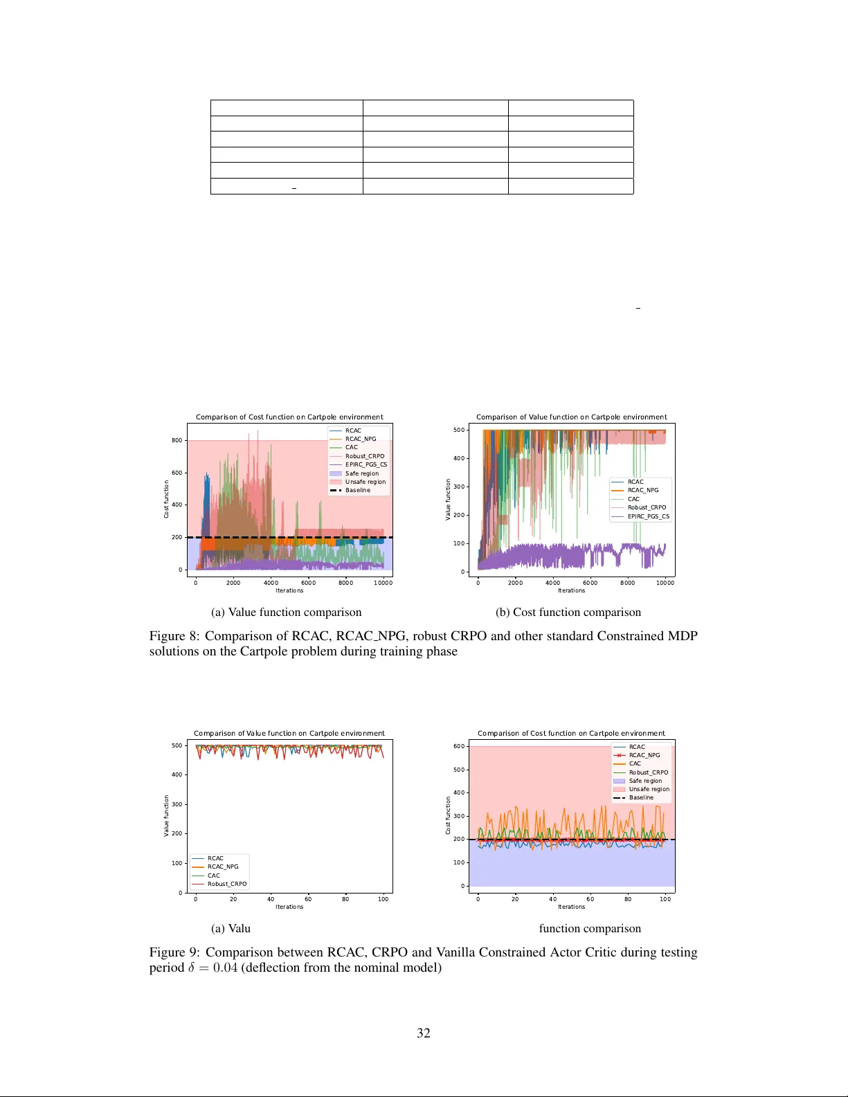
Efﬁcient P olicy Optimization in Rob ust Constrained MDPs with Iteration Complexity Guarantees Sourav Ganguly Department of ECE New Jerse y Institute of T echnology New Jerse y , USA sg2786@njit.edu Kishan Panaganti Department of CMS California Institute of T echnology (now at T encent AI Lab, Seattle, W A) kpb.research@gmail.com Arnob Ghosh Department of ECE New Jerse y Institute of T echnology New Jerse y , USA arnob.ghosh@njit.edu Adam Wierman Department of CMS California Institute of T echnology California, USA adamw@caltech.edu Abstract Constrained decision-making is essential for designing safe policies in real-w orld control systems, yet simulated environments often f ail to capture real-world ad- versities. W e consider the problem of learning a polic y that will maximize the cumulativ e rew ard while satisfying a constraint, ev en when there is a mismatch between the real model and an accessible simulator/nominal model. In particular, we consider the rob ust constrained Marko v decision problem (RCMDP) where an agent needs to maximize the rew ard and satisfy the constraint against the worst possible stochastic model under the uncertainty set centered around an unknown nominal model. Primal-dual methods, effecti v e for standard constrained MDP (CMDP), are not applicable here because of the lack of the strong duality prop- erty . Further , one cannot apply the standard rob ust v alue-iteration based approach on the composite value function either as the worst case models may be different for the reward value function and the constraint value function. W e propose a nov el technique that ef fecti vely minimizes the constraint value function–to satisfy the constraints; on the other hand, when all the constraints are satisﬁed, it can simply maximize the robust rew ard value function. W e prove that such an algo- rithm ﬁnds a policy with at most ϵ sub-optimality and feasible polic y after O ( ϵ − 2 ) iterations. In contrast to the state-of-the-art methods, we do not need to employ a binary search, thus, we reduce the computation time for larger value of discount factor ( γ ), and achiev e a better performance for large state space. 1 Introduction Ensuring safety or satisfying constraints is important for implementation of the RL algorithms in the real system. A poorly chosen action can lead to catastrophic consequences, making it crucial to incorporate safety constraints into the design. F or instance, in self-driving cars [1], a slight safety violation can result in serious harm to the system. Constrained Marko v Decision Process (CMDP) can address such safety concerns where the agent aims to maximize the expected re ward while k eep- ing the expected constraint cost within a predeﬁned safety boundary [2] (cf.(5)). CMDPs effecti vely restricted agents from violating safety limits [3, 4]. Ho we ver , in many practical problems, an al- gorithm is trained using a simulator which might be different from the real world. Thus, policies obtained for CMDP in simulated en vironment can still violate the constraint in the real en vironment. T o resolv e the abo ve issues, recently , researchers considered robust CMDP (RCMDP) problem where the constraint needs to be satisﬁed even when there is a model-mismatch due to the sim- Preprint. Under re view . W all-clock time comparisons (in secs) En vironment Name RNPG (our) EPIRC-PGS ( γ vals.) 0.9 0.99 0.995 CRS 48.574 190.53 228.65 290.15 Garnet 78.406 290.21 316.23 453.14 Modiﬁed Frozenlak e 160.31 453.7 561.47 620.12 Garbage collector 177.13 344.87 400.13 489.54 T able 1: Comparison of execution times av eraged over multiple runs between RNPG, and EPIRC-PGS (inner loop T = 100 and outer -loop K=10) (Some more e xperimental results to demonstrate f aster performance of our algorithms can be found in appendix G) to-real gap. In particular , we seek to solve the problem RCMDP objective: min π max P ∈ P J π ,P c 0 s.t. max P ∈ P J π ,P c i ≤ b, i ∈ { 1 , . . . , K } . (1) where J c n is the expected cumulativ e cost for the associated RCMDP cost function c n (see Sec- tion 2). Here P is the uncertainty set centered around a nominal (simulator) model described in (6). Note that learning the optimal policy for RCMDP are more challenging compared to the CMDP . In particular , the main challenge lies in the fact that the standard primal-dual based approaches, which achiev e pro v able sample comple xity results for the CMDP problems [5, 6], cannot achie ve the same for the robust CMDP problem as the problem may not admit strong duality e ven when the strict fea- sibility holds [7]. This is because the state occupanc y measure is no longer con vex as the worst-case transition probability model depends on the policy . Due to the same reason, ev en applying robust value iteration is not possible for the Lagrangian unlik e the non-robust CMDP problem. Recently , [8] proposed an epigraph approach to solve the problem in (1). In particular , they consid- ered min π ,b 0 b 0 s.t. J π c n − b n ≤ 0; n ∈ { 0 , . . . , K } . (2) Hence, the objective is passed on to the constraint with an objectiv e of how tight the constraint can be. [8] ﬁnds the optimal policy for each b 0 , and then optimized b 0 using a binary search. They showed that for each b 0 , the iteration complexity is O ( ϵ − 4 ) to ﬁnd the optimal policy . Note that one needs to ev aluate robust value function at every iteration for each b 0 which is costly operation especially when γ is large as it is evident by T able 1. Further , the binary search method only works when the estimation is perfect [9], thus, if the robust policy ev aluator is noisy which is more likely for the large state-space, the binary search method may not work as it is evident in our function approximation setup (Appendix G). Moreover , the complexity of iteration is only O (log( ϵ − 1 ) ϵ − 4 ) , which is worse than that of the CMDP [10]. W e seek to answer the following: Can we develop a computationally mor e efﬁcient (without binary searc h) ap- pr oac h for r obust CMDP pr oblem with a faster iteration comple xity bound? Our Contributions • W e propose a no vel approach to address the optimization problem. Speciﬁcally , we reformulate it as follows: min π max  J π c 0 λ , max n  J π c n − b n   . (3) This formulation balances the trade-off between optimizing the objective and satisfying the con- straints. When max n  J π c n − b n  > 0 , the focus is on reducing constraint violations. Otherwise, the objecti ve J π c 0 is minimized, scaled by the f actor λ . Notably , this framework eliminates the need for binary search over λ ; solving the abov e problem directly yields a policy that respects the con- straints for an appropriately chosen λ . W e sho w the almost equiv alence of optimal solution of (3) and (1). Howe ver , because of the point-wise maximum over the multiple objectives, it introduces additional challenges in achieving the iteration complexity , as the index of the value function of the objectiv e no w depends on the policy . • W e propose an algorithm (RNPG) that gives a policy which is at most ϵ -sub optimal and feasible after O ( ξ − 2 ϵ − 2 ) iterations if the strict feasibility parameter ξ is known. This is the ﬁrst result to show that strict safety feasibility can be achiev ed. This improv es the e xisting iteration comple xity 2 O (log  1 (1 − γ ) ϵ  ϵ − 4 ) achie ved by EPIRC-PGS by [8]. Our algorithm does not rely on binary search and uses KL regularization instead of projected gradient descent. W e also show that if we do not know ξ , we can achieve a policy that violates the constraint by at most ϵ amount while being at most ϵ -suboptimal with O (1 /ϵ 4 ) iteration complexity . Moreover , our dependence on the state-space ( S ) , and the effecti ve horizon (i.e., 1 1 − γ ) are much better compared to EPIRC-PGS. • W e extend our framework to the function approximation setup by proposing a robust constrained actor-critic with inte gral probability metric as the uncertainty metric. For the ﬁnite-state, our empirical results show that our proposed approaches achiev e a feasible policy with good reward (comparable or better than the one achiev ed by EPIRC-PGS, see T able 11) at a faster wall-clock time (see T able 1) 1 compared to the EPIRC-PGS. From T able 1, it is evident that our algorithm speeds up the computation process by at-least 2 times as compared to EPIRC-PGS algorithm when γ = 0 . 9 and at-least 3 times to EPIRC-PGS when γ = 0 . 995 . For the function approximation setup, our proposed approach is the only one that achieves feasibility and ev en a better rew ard to the robust v ersion of CRPO [11] during the test time for Cartpole e xperiment (T able 12). Further, we outperform EPIRC-PGS signiﬁcant manner for the function approximation setup both in terms of performance and the training time showing its ef ﬁcac y . 1.1 Related W orks CMDP: The con ve x nature of the state-action occupancy measure ensures the existence of a zero duality gap between the primal and dual problem for CMDP , making them well-suited for solution via primal-dual methods [2, 12–19]. The conv ergence bounds and rates of conv ergence for these methods hav e been extensiv ely studied in [20–24, 6, 25, 26]. Be yond primal-dual methods, LP- based and model-based approaches hav e been explored to solve the primal problem directly [27, 18, 28, 29, 11, 30]. Howe ver , the above approaches cannot be extended to the RCMDP case. Robust MDP: F or rob ust (unconstrained) MDPs (introduced in [31]), recent studies obtain the sample complexity guarantee using robust dynamic programming approach [32 – 36]. Model-free approaches are also studied [34, 37 – 43]. Howe ver , extending these methods to Rob ust Constrained MDPs (RCMDPs) presents additional challenges. The introduction of constraint functions com- plicates the optimization process as one needs to consider the worst value function both for the objectiv e and the constraint. RCMDP: Unlike non-robust CMDPs, there is limited research av ailable on robust en vironments. In [7], it was shown that the optimization function for RCMDPs is not conv ex, making it difﬁcult to solve the Lagrangian formulation, unlike in standard CMDPs. Some studies have attempted to address this challenge using a primal-dual approach [44, 7] without any iteration comple xity guarantee. [45] proposed a primal-dual approach to solve RCMDP under the strong duality by restricting to the categorical randomized policy class. Howe ver , they did not provide any iteration complexity guarantee. As we discussed, [8] reformulates the Lagrangian problem into an epigraph representation, addressing the limitations of previous methods while providing valuable theoretical insights. Ho wev er , this method requires a binary search, signiﬁcantly increasing computational complexity . Moreover , the binary search approach fails when the estimated robust policy value function is noisy [9]. 2 Problem F ormulation CMDP: W e denote a MDP as M = ⟨S , A , P , C , { c j } K j =1 , γ ⟩ where S , A , P : S × A × S → R denote state space, action space, and probability transition function respectively . γ ∈ [0 , 1) denotes the discount factor and c i : S × A → R , for i = { 0 , 1 , . . . , K } , denotes the constraint function. Let R + = max (0 , R ) for any real number R and π : S → A denote a policy . Let β : S → ∆( S ) denote the initial state distrib ution where ∆( S ) denotes the probability distrib ution tak en o ver space S . Let V P,π c i ( s ) : S → R , s.t. i ∈ { 0 , . . . , K } (where c 0 ∈ C denote the cost for the objectiv e) denote the value function obtained by follo wing polic y π and the transition model P where V π ,P c i ( s ) := E P,π  ∞ Σ t =1 γ t − 1 π ( a | s ) c t i ( s, a )  , (4) 1 The system speciﬁcations are, Processor: Intel(R)Core(TM)i7-14700-2.10 GHz, Installed RAM 32.0 GB (31.7 GB usable),64-bit operating system, x64-based processor No GPU. 3 where c t i ( s, a ) denotes the single step ‘ i ’th-cost/re ward for being at a state ‘ s ’ and taking action ‘ a ’ at the ‘ t ’-th instant. W ithout loss of generality , we assume 0 ≤ c i ( s, a ) ≤ 1 s.t. i ∈ { 0 , . . . , K } . This is in consistent with the e xisting literature [8]. W e also denote J P,π c i = ⟨ ρ, V P,π c i ⟩ for i ∈ { 0 , . . . , K } where ρ is the initial state-distribution. F or notational simplicity , we denote H = 1 / (1 − γ ) as the maximum cost value. The MDP M forms a constrained MDP when constraint cost functions are bounded by a threshold, leading to the following optimization problem, CMDP objective: min J π ,P c 0 s.t. J π ,P c i ≤ b i ∀ i ∈ { 1 , . . . , K } . (5) Note that even though we consider a cost-based en vironment to be consistent with the RCMDP literature [8] where the objective is to minimize the expected cumulative cost, our analysis can easily go through for reward-based environment where the objective is to maximize the expected cumulativ e re ward. Further , we can also consider the constraints of the form J π ,P c i ≥ b i . RCMDP: W e consider that we hav e access to the nominal model P 0 , ho we ver , the true model might be different compared to the nominal model P 0 . Such a scenario is relev ant when we train using simulator , howe ver , the real en vironment might be dif ferent compared to the simulator . The state- of-the art choice for the uncertainty set is to collect all the probability distribution which are in close proximity to a nominal model P 0 ∈ ∆( S × A ) . Thus P = N ( s,a ) ∈S ×A P ( s,a ) such that P ( s,a ) = { P ∈ ∆( S ) : D ( P, P 0 ( s, a )) ≤ ρ } , (6) where D ( ., . ) is the distance measure between two probability distribution and ρ denotes the max- imum perturbation possible from the nominal model. Some poplar choices for D ( ., . ) are TV dis- tance, χ 2 distance and KL-div ergence [32]. Equation (6) satisﬁes the ( s, a ) -rectangularity assumption. It is important to note that our analy- sis and algorithm remain applicable as long as a robust policy e valuator , that is, max P ∈P J π ,P c i is av ailable. Therefore, we can also extend our approach to consider s -rectangular uncertainty sets. In addition, it is possible to e xtend this to the integral probability metric (IPM). Howe ver , without such an assumption, ev aluating a rob ust v alue function becomes an NP-hard problem. The objectiv e in constrained robust MDPs is to minimize (or maximize in a reward based setting) the worst case value function while keeping the worst case expected cost function within a thresh- old (user deﬁned) as deﬁned in (1). W e denote max P J P,π c i = J π c i as the worst possible expected cumulative cost corr esponding to cost c i following the policy π . Learning Metric : Since we do not know the model, we are in the data-driv en learning setting. Here, we are interested in ﬁnding the number of iterations ( T ) required to obtain a policy ˆ π with sub-optimality gap of at most ϵ , and a feasible policy incurring no violations. That is, after T iterations, ˆ π satisﬁes Gap( ˆ π ) = J ˆ π c 0 − J π ∗ c 0 ≤ ϵ and Violation( ˆ π ) = max n J ˆ π c n − b n ≤ 0 , (7) where π ∗ is the optimal policy of (1). Note that we do not assume an y restriction on the polic y class Π unlik e in [8]. In [45], the policy class increases as T increases as it is an ensemble of the learned policies up to time T . Here, Π denotes an y Markovian polic y . Thus, the iteration complexity measures how many iterations required to obtain a feasible policy with sub-optimality gap of at most ϵ . Iteration complexity is a standard measure for unconstrained robust MDP [38]. In addition to sub-optimality gap, we also seek to achieve a feasible policy ˆ π for RCMDP . Note that unlik e in [8], where they allowed a violation of ϵ , here, we want to ﬁnd a feasible policy , a stricter requirement. Difﬁculty with the vanilla primal-dual method The most celebrated method to solv e a constrained optimization problem is by introducing Lagrangian multiplers. Let us consider λ = ( λ 1 . . . λ K ) ∈ R N + be the set of langrangian multipliers introduced to conv ert the primal problem eqn. (1) into the dual space which is shown in eqn. (8) J ∗ = min π ∈ Π max λ ∈ R N + max P ∈ P J π ,P c 0 + N Σ i =1 λ i . max P ∈ P ( J π ,P c i − b i ) . (8) In the CMDP problem, [46] shows that the strong duality holds when there exists a strictly feasible policy (aka Slater’ s condition). Howe ver , a concurrent work [47] highlighted that strong duality 4 does not hold for the RCMDP problem as the occupancy measure is no longer conv ex as the worst transition model dif fers for different policies. In addition to that, in [8] a strong ambiguity reg arding the tractability in solving lagrangian problem is discussed. Further , ev en if one ﬁxes λ , one cannot apply robust value iteration approach to ﬁnd the optimal polic y for the Lagrangian unlike the CMDP . Hence, it is evident to look for alternati v e measures to ﬁnd a solution to the optimality problem. 3 Policy Gradient A pproach f or RCMDPs In this section, we discuss our approach to solve the RCMDP problem (eqn.(1)). In what follows, we describe our policy optimization algorithm RNPG in detail. 3.1 Our Proposed A ppr oach In order to address the challenges of the primal-dual problem, W e consider the following problem min π max { J π c 0 /λ, max n [ J π c n − b n ] } . (9) Intuition : Note that when J π c i ≤ b i for all i = 1 , . . . , K , the second term in the objectiv e becomes negati v e, and since J π c 0 ≥ 0 , the optimization will focus on minimizing J π c 0 , as the policy is likely to be feasible with respect to all constraints. Con versely , if there exists any i such that J π c i > b i , then for a suf ﬁciently lar ge λ , the term J π c 0 /λ becomes smaller than J π c i − b i , causing the optimization to prioritize reducing the most violated constraint J π c i . Even though we can not claim that (9) and (1) are the same, we can claim that the optimal solution of (9) can only violate the constraint by at most ϵ -amount by a suitable choice of λ . Hence, minimizing (9) amounts to searching for policies that can violate at most ϵ amount. Thus, the optimal policy of (1) can be an optimal of (9). In particular , optimal policy of (9) indeed has a smaller cost compared to that of (1). W e formalize this as the following result. Proposition 1. Suppose that ˆ π ∗ is the optimal policy of (9) then J ˆ π ∗ c 0 ≤ J π ∗ c 0 , and can only violate the constraint by at most ϵ with λ = 2 H /ϵ . The key distinction from the epigraph-based approach proposed in [8] is that we avoid tuning the hyperparameter b 0 via binary search. This signiﬁcantly reduces computational ov erhead, as also demonstrated in our empirical ev aluations. Furthermore, tuning b 0 typically requires accurate esti- mation, ev en an unbiased estimation would not work, which is prohibitiv e as the state-space grows when a high-probability estimate becomes challenging. Since our goal is to obtain a feasible policy , we assume that the optimal policy is strictly feasible. Assumption 1. W e assume that max n J π ∗ c n − b n ≤ − ξ , for some ξ > 0 . The above assumption is required because we want to have a feasible policy rather bounding the violation gap to ϵ . Note that we only need to know (or, estimate) the value of ξ . Of course, we do not need to know the optimal policy π ∗ . Using ξ , we can show that we achieve a feasible policy with at most ϵ -gap in Theorem 4.1. Intuitiv ely , if ξ > ϵ , it means that by choosing λ = 2 H /ξ , we can actually guarantee feasibility according to Proposition 1. W e relax this ξ -dependency in Theorem 6.1 where we show that we can achie v e a policy with at most ϵ -gap and ϵ -violation. W e consider the problem min π max { J π c 0 /λ, max n J π c n − b n + ξ } . (10) Note that ev en though for theoretical analysis to achie ve a feasible polic y we assume the kno wledge of ξ ; for our empirical e valuations, we did not assume that and yet we achiev ed feasible policy with good rew ard exceeding the state-of-the-art performance. Hence, we modify the policy space to be ξ -dependent. 3.2 Policy Optimization Algorithm W e now describe our proposed robust natural policy gradient (RNPG) approach inspired from the unconstrained natural polic y gradient [48]. For notational simplicity , we deﬁne J i ( π ) = J π c i − b i + ξ for i = 1 , . . . , K , and J 0 ( π ) = J π c 0 /λ . The policy update is then giv en by– π t +1 ∈ arg min π ∈ Π ⟨∇ π t J i ( π t ) , π − π t ⟩ + 1 α t KL( π || π t ) where i = arg max { J π c 0 λ , { J π c n − b n + ξ } K n =1 } 5 where KL is the usual K ullback-Leibler di ver gence. Note that this is a conv ex optimization problem, and can be optimized ef ﬁciently . If we use, ℓ 2 regularization, i.e., || π − π t || 2 2 , then it becomes a rob ust projected polic y gradient (RPPG) adapted from the unconstrained version (see Appendix D) [49, 38], a v ariant of which is used in [8] to ﬁnd optimal policy for each b 0 . Of course, our approach also works for ℓ 2 norm which we deﬁne in Algorithm 4. Empirically , we observe that KL-di v ergence has a better performance, and provide iteration comple xity for RNPG. The complete procedure is described in Algorithm 1. First, we ev aluate J π t c i and ∇ π t J π t c i using the robust polic y e valuator which we describe in the follo wing. Robust Policy Evaluator: Our algorithm assumes access to a robust policy e valuation oracle that returns the worst-case performance of a given policy , i.e., J π c i = max P ∈ P J π ,P c i . This assumption is standard and is also adopted in both constrained [8] and unconstrained [38] robust MDP framew orks. As we discussed, se v eral ef ﬁcient techniques exist for ev aluating rob ust policies under v arious uncer - tainty models especially with ( s, a ) rectangular assumption (6). In this work, we focus on the widely studied and expressi ve KL-divergence-based uncertainty set , which not only captures an inﬁnite family of plausible transition models b ut also admits a closed-form robust e v aluation method. The robust v alue function under the KL-uncertainty set is formalized in Lemma D.1 (see Ap- pendix D). The advantage is that we obtain a closed form expression for the robust value function, and we can ev aluate it by drawing samples from the nominal model only . For further background on KL and other uncertainty sets, we refer the reader to [50, 34, 33]. Our framew ork is not limited to KL-diver gence. Ef ﬁcient robust value function ev aluation tech- niques exist for other popular uncertainty models such as T otal V ariation (TV), W asserstein, and χ 2 -div ergence sets [32, 51, 52, 33]. These approaches typically lev erage dual formulations to efﬁ- ciently solv e the inner maximization problem required for rob ust ev aluation. W e need our robust pol- icy ev aluator to be only ϵ -accurate. For many uncertainty sets including popular ( s, a ) -rectangular perturbation (e.g., KL-div ergence, TV -distance, χ 2 uncertainty sets) this requires O (1 /ϵ 2 ) samples [32, 34]. Hence, we need T ϵ − 2 samples in those cases. Policy Update : In order to ev aluate ∇ π t J π i , we use the following result directly adapted to our setting from [48] Lemma 3.1. F or any π ∈ Π , transition kernel P : S × A → ∆( S ) , for i = 1 , . . . , K ( ∇ J i,P ( π ))( s, a ) = 1 1 − γ d π P ( s ) Q π i,P ( s, a ) , wher e Q π i,P ( s, a ) = Q π c i ,P , and Q 0 ,P = Q π c 0 ,P /λ . Consider i t = arg max { J π t c 0 /λ, { J π t c i − b i + ξ } K i =1 } , and p t = arg max J π t ,p t c i t , we can ev aluate ∇ π t J π t ,p t c i t using the robust e v aluator for Q π t ,p t c i t ( · , · ) as mentioned. Hence, the natural policy update at iteration t can be decomposed as multiple independent Mirror Descent updates across the states– π t +1 ,s = arg min ∆ A {⟨ Q π t ,p t i t , π s ⟩ + 1 α t K L ( π s || π t,s ) } , ∀ s. (11) Again, this is ef ﬁcient since it is con ve x. W e use direct parameterization and soft-max parameteriza- tion for the policy update (Appendix F) by solving the optimization problem (11). The Algorithm 1 outputs π ∗ t corresponding to the minimum objectiv e over T iterations. W e characterize T , the itera- tion complexity in the ne xt section. Although Algorithm 1 includes ξ for theoretical analysis, we do not assume knowledge of ξ in our empirical e valuations. In Section 6, we discuss how we ac hieve a slightly weaker iter ation comple x- ity r esult without assuming the knowledge of ξ . 4 Theoretical Results In this section, we will discuss the results obtained for our RNPG algorithm (Algorithm 1). Before describing, the main results, we state the Assumptions. Assumption 2. There e xists β ∈ (0 , 1) such that γ p ( s ′ | s, a ) ≤ β p 0 ( s ′ | s, a ) ∀ s ′ , s, a, and p ∈ P . This w as a common assumption for unconstrained RMDP as well [53, 54]. Assumption 2 states that if the perturbed distribution assigns positive probability to an ev ent, the nominal model should also 6 Algorithm 1 Robust-Natural Polic y Gradient for constrained MDP (RNPG) Input: α , λ , T , ρ , V ( . ) (Rob ust Policy Ev aluator , see Algorithm 2)) Initialize: π 0 = 1 / | A | . for t = 0 . . . T − 1 do J π t c i , ∇ J π t c i = V ( c i , ρ ) where i = { 0 , 1 , . . . , K } . Update π t +1 according to (11). end for Output policy arg m in π t s.t.t ∈{ 0 ,...,T − 1 } max { J π t c 0 /λ, max i ( J π t c i − b i + ξ ) } . assign positiv e probability to that ev ent. Otherwise, a mismatch in supports could lead to unsampled regions and render ﬁnite-iteration bounds intractable. More importantly , Algorithm 1 does not need to know β . W e also did not enforce in our empirical studies. The algorithm still performed well, suggesting that the practical impact may be less restrictive than the theory implies. Also, EPIRC- PGS [8] assumed that the ratio between the state-action occupancy measures on the states covered by all policies and the initial state distribution is bounded. W e also consider a slightly stronger optimal policy for the surrogate problem. Assumption 3. W e consider ˆ π ∗ ,a uniform minimizer acr oss all states of the surro gate pr oblem in (9), i.e., ˆ π ∗ is a solution of min π max { V π ,P c 0 ( s ) /λ, max n max P V π ,P c i − b n } for all s . A similar assumption is also considered for the unconstrained problem [54, 31]. Theorem 4.1. Under Assumptions 1, 2, and 3 with λ = 2 H / min { ξ , 1 } , α t = α 0 = 1 − γ √ T S after T = O ( ϵ − 2 ξ − 2 (1 − γ ) − 2 (1 − β ) − 2 S log( | A | )) iterations, Algorithm 1 r eturns a policy ˆ π such that J ˆ π r − J π ∗ r ≤ ϵ , and max n J ˆ π c n − b n ≤ 0 . Thus, Algorithm 1 has an iteration complexity of O ( ϵ − 2 ) . Also, the policy is feasible and only at most ϵ -sub optimal. Our result improv es upon the result O ( ϵ − 4 ) achiev ed in [8]. Further, they did not guarantee feasibility of the policy (rather, only ϵ -violation). More importantly , we do not need to employ a binary search algorithm. Thus, our algorithm is computationally more efﬁcient. Our dependence on S , A , and (1 − γ ) − 1 ar e signiﬁcantly better compared to [8] as well. Note that for the unconstrained case the iteration complexity is O ( ϵ − 1 ) [48]; whether we can achie ve such a result for robust CMDP has been left for the future. As we mentioned, we do not use this ξ for our empirical ev aluations. Y et our results indicate that we can achiev e feasible policy with better performance compared to EPIRC-PGS in signiﬁcantly smaller time. In Section 6, we also obtain the result when we relax Assumption 1 with slightly worse iteration complexity by simply putting ξ = 0 , and λ = 2 H /ϵ . 4.1 Proof Outline The proof will be di vided in two parts. First, we bound the iteration complexity for ϵ -sub optimal solution of (10). Subsequently , we show that the sub-optimality gap and violation gap using the abov e result. Bounding the Iteration complexity for (10) : The follo wing result is the ke y to achiev e the iteration complexity result of Algorithm 1 for the Problem (10) Lemma 4.2. The policy ˆ π r eturned by Algorithm 1 satisﬁes the following pr operty: max { J ˆ π c 0 /λ, max n J ˆ π c n − b n } − max { J π c 0 /λ, max n J π c n − b n } ≤ ϵ/λ (12) for any policy π after O ( λ 2 ϵ − 2 (1 − γ ) − 4 (1 − β ) − 2 ) iter ations under Assumptions 2, and 3. Hence, the above result entails that Algorithm 4 returns a policy which is at most ϵ -suboptimal for the problem (10) after O ( ϵ − 2 ξ − 2 ) . W e show that using this result we bound the sub-optimality and the violation gap. T echnical Challenge : The main challenge compared to the policy optimization-based approaches for unconstrained RMDP is that here the objectiv e (cf.(9)) is point-wise maximum of multiple value 7 functions for a particular policy . Hence, one might be optimizing different objecti ves at dif ferent it- erations at π t is varying across the iterations. Hence, unlike the unconstrained case, we cannot apply the robust robust performance difference Lemma as the value-function index might be different for π t , and π t +1 . Instead, we bound it using Assumption 2, Holder’ s, and Pinsker’ s inequality . Bounding the Sub-optimality Gap : By Assumption 1, J π ∗ c n ≤ b n − ξ . Hence, max n J π ∗ c n − b n + ξ ≤ J π ∗ c 0 /λ as J π ∗ c 0 ≥ 0 . Thus, ( J ˆ π c 0 − J π ∗ c 0 ) /λ ≤ max { J ˆ π c 0 /λ, max n J ˆ π c n − b n + ξ } − max { J π ∗ c 0 /λ, max n J π ∗ c n − b n + ξ } ≤ ϵ/λ (13) where the last inequality follows from Lemma 4.2. By multiplying both the sides by λ , we have the result. Bounding the V iolation : W e now bound the violations. max n ( J ˆ π c n − b n + ξ ) ≤ max n ( J ˆ π c n − b n + ξ ) − J π ∗ c 0 /λ + H /λ ≤ max { J ˆ π c 0 /λ, max n J ˆ π c n − b n } − max { J π ∗ c 0 /λ, max n J π ∗ c n − b n + ξ } + H /λ ≤ ξ / 2 + ϵ/λ ≤ ξ , (14) where for the ﬁrst inequality , we use the fact that J π ∗ c 0 /λ ≤ H /λ . For the secnond inequality , we use the fact that J π ∗ c n ≤ b n − ξ . Hence, max n J π ∗ c n − b n + ξ ≤ J π ∗ c 0 /λ . Since λ ≥ 2 H /ξ , thus, H /λ ≤ ξ / 2 . Note that ϵ/λ = ϵ min { ξ , 1 } / (2 H ) ≤ ϵξ / (2 H ) ≤ ξ / 2 . Hence, the above shows that max n ( J ˆ π c n − b n ) ≤ 0 . 5 Experimental Results W e ev aluate our algorithms 2 on two en vironments: (i) Garnet , and (ii) Constr ained Riverswim (CRS) . Additional experimental results are pro vided in Appendix E. W e have ﬁxed λ = 50 across the en vironments. This demonstrates that with the inclusion of a KL regularization term over policy updates, RNPG eliminates the need for manual tuning of λ . A sufﬁciently large ﬁxed value ( λ = 50 ) yields consistently strong performance. For a detailed description of the hyperparameters used, please refer to Appendix E. Garnet: The Garnet en vironment is a well-known RL benchmark that consists of nS states and nA actions, as described in [55]. For our experiments, we consider G (15 , 20) with 15 states and 20 ac- tions. The nominal pr obability function , r ewar d function , and utility function are each sampled from separate normal distributions: N ( µ a , σ a ) , N ( µ b , σ b ) , and N ( µ c , σ c ) , where the means µ a , µ b , and µ c are drawn from a uniform distribution U nif (0 , 100) . T o ensure valid probability distributions, the nominal probabilities are exponentiated and then normalized. In this en vironment, we seek to maximize the rew ard while ensuring that the constraint is abov e a threshold. 0 200 400 600 800 1000 Iteration 0 50 100 150 200 Cumulative Objective r ewar d Objective function RNPG RPPG EPIR C 0 200 400 600 800 1000 Iteration 0 20 40 60 80 100 120 Cumulative constraint cost Constraint function RNPG RPPG EPIR C baseline Safe r egion Unsafe R egion Figure 1: Comparison of RNPG, RPPG and EPIRC-PGS on Garnet(15,20) environment. Here, we want to maximize the objectiv e (vf), and want the constraint (cf) to be abov e the baseline. Constrained River -swim (CRS): The Riv er-Swim en vironment consists of six states, each repre- senting an island in a water body . The swimmer begins at any island and aims to reach either end 2 The complete implementation is av ailable at https://github.com/Sourav1429/RCAC_NPG.git 8 of the riv er to earn a reward. At each state, the swimmer has two possible actions: swim left ( a 0 ) or swim right ( a 1 ). Rew ards are only provided at the boundary states, while intermediate states do not offer any rewards. The leftmost state, s 0 , and the rightmost state, s 5 , correspond to the riv erbanks. As the swimmer moves from s 0 to s 5 , the water depth increases, and dangerous whirlpools become more prev alent. This progression is captured by a safety constraint cost , which varies across states. The safety cost is lowest at s 0 and reaches its maximum at s 5 , reﬂecting the increasing risk as the swimmer ventures further downstream. Here the goal is to maximize the cumulati ve reward while ensuring the cumulativ e cost is belo w a threshold. 0 200 400 600 800 1000 Iteration 0 20 40 60 80 100 120 Cumulative Objective r ewar d Objective function RNPG RPPG EPIR C 0 200 400 600 800 1000 Iteration 20 25 30 35 40 45 50 Cumulative constraint cost Constraint function RNPG RPPG EPIR C baseline Unsafe r egion Safe R egion Figure 2: Comparison of RPPG and EPIRC-PGS on CRS environment. Here we want to maximize the objectiv e (vf) while constraint (cf) being below the threshold line. 5.1 Analysis of results • Does RNPG perform better than EPIRC-PGS? Perf ormance : Our experimental results demonstrate that RNPG consistently outperforms EPIRC- PGS, in both en vironments. In fact, for the CRS en vir onment (F igure 2) RNPG is the only one that pr oduces a feasible policy . EPIRC-PGS is unable to produce a feasible policy there. In the Garnet en vironment (Figure 1), RNPG ﬁnds a feasible policy while achieving a better reward compared to the EPIRC-PGS. Also, RNPG shows a better con ver gence property and is more stable because of the KL regularization. Computational Time : RNPG exhibits signiﬁcant improv ements in computational efﬁcienc y , achieving conv ergence at least 4x f aster than EPIRC-PGS for γ = 0 . 9 , and 6x faster for γ = 0 . 995 in the CRS setting (T able 1). In the Garnet en vironment, RNPG achiev es a 3x speedup ov er EPIRC-PGS for γ = 0 . 9 , and at least 5x speedup for γ = 0 . 995 (T able 1). The difference in runtime can be attributed to the fact that RNPG eliminates the need for binary search for each b 0 value in (2) as described abo ve, and it uses a KL re gularization. T o summarize, RNPG performs better compared to EPIRC-PGS in terms of achieving a better rew ard while maintaining feasibility across the en vironments. Moreover , the con vergence is stable across the en vironments, and reduces the computational time signiﬁcantly compared to EPIRC- PGS as theoretical result suggested. • KL re gularization compared to ℓ 2 r e gularization. W e also compare RNPG with RPPG (see Appendix D), a projected robust gradient descent v ariant that uses an ℓ 2 regularizer instead of KL for polic y update in (11). In the CRS en vironment, RPPG performs slightly better than EPIRC-PGS by maintaining smaller constraint violations, though it still occasionally breaches the safety threshold. In the Garnet en vironment, RPPG achieves a better performance compared to EPIRC-PGS while maintaining feasibility , howe ver , it achiev es a smaller re ward compared to RNPG. RNPG is also much stable, sho wing that KL regularization is more ef fectiv e compared to ℓ 2 regularization. W e observe that RPPG (and, similar to RNPG) also has a smaller computational time compared to EPIRC-PGS, which demonstrates that removing the binary search is the key , as EPIRC-PGS also uses ℓ 2 regularization for polic y update. • Does λ r equir e extensive tuning for RNPG? A particularly notable observation from our experiments is that RNPG performs robustly across different en vironments using a ﬁx ed v alue of λ = 50 . This highlights that RNPG does not need to set different λ values for different en vironments as theoretical result suggested. Rather , one high λ -value is enough to achie v es feasibility while achieving good re ward. 9 6 Discussions and Limitation Relaxing Assumption 1 : W e achieve our results in Theorem 4.1 where we assume that the optimal policy is strictly feasible and the feasibility parameter ξ is kno wn. W e will relax both the features of the assumption that ξ is known, and the optimal policy is strictly feasible in the follo wing with a slightly worse iteration complexity while ensuring that the policy has violation of at most ϵ , the same metric achiev ed by EPIRC-PGS [8]. Theorem 6.1. Algorithm 1 gives a policy ˆ π such that J ˆ π c 0 − J π ∗ c 0 ≤ ϵ and max n J ˆ π c n − b n ≤ ϵ after O ( ϵ − 4 (1 − γ ) − 4 (1 − β ) − 2 log( | A | )) number of iter ations when we plug λ = 2 H /ϵ and ξ = 0 . Note that since we are not assuming strict feasibility of the optimal policy , we can only bound the violation up to ϵ . The ke y here is to use λ = 2 H/ϵ as we do not know ξ , and then obtain an ϵ 2 -close result using Lemma 4.2. This makes the iteration complexity of O ( ϵ − 4 ) . Note that our dependence on S , A , and 1 / (1 − γ ) are signiﬁcantly better compared to EPIRC-PGS[8]. Further, we do not employ binary search. The proof is in Appendix C. 6.1 Extending to Function Appr oximation: Robust Constrained Actor -Critic (RCA C) W e extend our framework to the function approximation setting moti vated by the work of [54] for unconstrained Rob ust MDP problem. In particular , we consider the integral probability metric (IPM) as an uncertainty set, d F ( p, q ) = sup f ∈F { p T f − q T f } where F ⊆ R | S | . Many metrics such as Kantorovich metric, total v ariation, etc., are special cases of IPM under dif ferent function classes [56]. W e then consider the IPM-based uncertainty set, P s,a = { q | d F ( q , p 0 s,a ) ≤ ρ } around the nominal model. Consider the linear function approximation setting where V π c i ,w = Ψ w π c i where Ψ ∈ ℜ | S |× d is a feature matrix of ψ T ( s ) ∀ s as each row . W e now consider the following function class F = { s → ψ ( s ) T ζ , ζ ∈ ℜ d , || ζ || 2 ≤ 1 } . Now , we can apply the Proposition 1 in [57] to achieve the worst case value function. In particular , we hav e sup q ∈ d F ( q ,p 0 s,a ) q T V π c i ,w = ( p 0 s,a ) T V π c i ,w + ρ || w π c i , 2: d || 2 where we normalize to let the ﬁrst coordinate of ψ ( s ) = 1 . Hence, we can use the following equation to compute the robust Bellman operator L P V π c i ,w = c i ( s, a ) + γ V π c i ,w + ρ || w c i , 2: d || 2 , (15) with the next state s ′ is drawn from the nominal model. Guided by the last regularization term of the empirical robust Bellman operator in (15), when considering value function approximation by neural networks we add a similar regularization term for all the neural network parameters except for the bias parameter in the last layer . W e use the expression in (15) for the robust value function for the gradient, and J c i in Algorithm 1. W e need to estimate the robust Q function. In order to estimate the Q -function we ﬁrst use (15) by plugging the V -approximation, and then we use the linear regression to ﬁt the critic for the rob ust Q -function. The details can be found in Appendix G. From the empirical results in Figure 9 and T able 12, it is evident that our proposed approach outper - forms the state-of-the-art approaches. More importantly , compared to the EPIRC-PGS (adapted to the function approximation setting), our approach achiev es a signiﬁcantly better performance with small w all-clock time. Also, our proposed approach outperforms the rob ust version of the CRPO al- gorithm [11, 47] and achie ves feasibility unlike robust CRPO. In Appendix H we sho wed that robust CRPO may not achiev e a ﬁnite time iteration complexity guarantee e v en for ﬁnite-state space. 7 Conclusions and Future W orks In this work, we present a novel algorithm that lev erages the projected policy gradient and natural policy gradient techniques to ﬁnd an ϵ -suboptimal and a feasible policy after O ( ϵ − 2 ) iterations for RCMDP problem. W e demonstrate the practical applicability of our algorithm by testing it on sev- eral standard reinforcement learning benchmarks. The empirical results highlight the effecti v eness of RNPG, particularly in terms of reduced computation time and achieving feasibility and a better rew ard compared to other state-of-the-art algorithms for RCMDP . Relaxing Assumption 2, and 3 constitute an important future research direction. Achieving a lower bound or improving the iteration complexity is also an important future research direction. Charac- terizing the results for other uncertainty sets also constitutes an important future research direction. Iteration complexity guarantee for the function approximation setting has been left for the future. 10 Acknowledgments A G and SG acknowledge NJIT Startup Fund index ed 172884. SG acknowledges Neurips 2025 for awarding him with the NeurIPS 2025 Scholar A ward. A W and KP acknowledge NSF grants CCF- 2326609, CNS-2146814, CPS-2136197, CNS-2106403, and NGSDI-2105648 and support from the Resnick Sustainability Institute. KP also ackno wledges support from the ‘PIMCO Postdoctoral Fel- low in Data Science’ fello wship at the California Institute of T echnology and the Resnick Institute. References [1] Ran Emuna, A vinoam Borowsk y , and Armin Biess. Deep reinforcement learning for human-like driving policies in collision avoidance tasks of self-driving cars. arXiv preprint arXiv:2006.04218 , 2020. [2] Eitan Altman. Constrained markov decision processes with total cost criteria: Lagrangian approach and dual linear program. Mathematical methods of operations resear c h , 48:387– 417, 1998. [3] Shuang Qiu, Xiaohan W ei, Zhuoran Y ang, Jieping Y e, and Zhaoran W ang. Upper conﬁdence primal-dual optimization: Stochastically constrained markov decision processes with adver- sarial losses and unknown transitions. arXiv preprint , 2020. [4] Sindhu Padakandla, KJ Prabuchandran, Sourav Ganguly , and Shalabh Bhatnagar . Data efﬁcient safe reinforcement learning. In 2022 IEEE International Conference on Systems, Man, and Cybernetics (SMC) , pages 1167–1172. IEEE, 2022. [5] Sharan V aswani, Lin F Y ang, and Csaba Szepesv ´ ari. Near-optimal sample complexity bounds for constrained mdps. arXiv pr eprint arXiv:2206.06270 , 2022. [6] Arnob Ghosh, Xingyu Zhou, and Ness Shroff. Prov ably efﬁcient model-free constrained rl with linear function approximation. Advances in Neural Information Pr ocessing Systems , 35: 13303–13315, 2022. [7] Y ue W ang, Fei Miao, and Shaofeng Zou. Robust constrained reinforcement learning. arXiv pr eprint arXiv:2209.06866 , 2022. [8] T oshinori Kitamura, T adashi K ozuno, W ataru K umagai, K enta Hoshino, Y ohei Hosoe, Kazumi Kasaura, Masashi Hamaya, Paav o Parmas, and Y utaka Matsuo. Near-optimal policy identiﬁ- cation in rob ust constrained marko v decision processes via epigraph form. arXiv pr eprint arXiv:2408.16286 , 2024. [9] Michael Horstein. Sequential transmission using noiseless feedback. IEEE T ransactions on Information Theory , 9(3):136–143, 1963. [10] Jiashuo Jiang and Y inyu Y e. Achieving o (1 /ϵ ) sample complexity for constrained markov decision process. arXiv pr eprint arXiv:2402.16324 , 2024. [11] T engyu Xu, Y ingbin Liang, and Guanghui Lan. Crpo: A new approach for safe reinforcement learning with conv ergence guarantee. In International Confer ence on Mac hine Learning , pages 11480–11491. PMLR, 2021. [12] Santiago Paternain, Miguel Calvo-Fullana, Luiz FO Chamon, and Alejandro Ribeiro. Safe policies for reinforcement learning via primal-dual methods. IEEE T ransactions on A utomatic Contr ol , 68(3):1321–1336, 2022. [13] Adam Stooke, Joshua Achiam, and Pieter Abbeel. Responsiv e safety in reinforcement learning by pid lagrangian methods. In International Conference on Machine Learning , pages 9133– 9143. PMLR, 2020. [14] Qingkai Liang, Fanyu Que, and Eytan Modiano. Accelerated primal-dual policy optimization for safe reinforcement learning. arXiv pr eprint arXiv:1802.06480 , 2018. [15] Chen T essler , Daniel J Manko witz, and Shie Mannor . Re ward constrained polic y optimization. arXiv pr eprint arXiv:1805.11074 , 2018. 11 [16] Ming Y u, Zhuoran Y ang, Mladen K olar , and Zhaoran W ang. Conv ergent policy optimization for safe reinforcement learning. Advances in Neur al Information Pr ocessing Systems , 32, 2019. [17] Liyuan Zheng and Lillian Ratliff. Constrained upper conﬁdence reinforcement learning. In Learning for Dynamics and Contr ol , pages 620–629. PMLR, 2020. [18] Y onathan Efroni, Shie Mannor, and Matteo Pirotta. Exploration-exploitation in constrained mdps. arXiv pr eprint arXiv:2003.02189 , 2020. [19] Peter Auer , Thomas Jaksch, and Ronald Ortner . Near-optimal re gret bounds for reinforcement learning. Advances in neural information pr ocessing systems , 21, 2008. [20] Dongsheng Ding, Kaiqing Zhang, T amer Basar, and Mihailo R Jo vano vic. Natural policy gradient primal-dual method for constrained markov decision processes. In NeurIPS , 2020. [21] Tianjiao Li, Ziwei Guan, Shaofeng Zou, T engyu Xu, Y ingbin Liang, and Guanghui Lan. Faster algorithm and sharper analysis for constrained markov decision process. Operations Resear ch Letters , 54:107107, 2024. [22] T ao Liu, Ruida Zhou, Dileep Kalathil, PR Kumar , and Chao Tian. Policy optimization for constrained mdps with prov able fast global conv ergence. arXiv preprint , 2021. [23] Donghao Y ing, Y uhao Ding, and Jav ad Lavaei. A dual approach to constrained markov de- cision processes with entropy regularization. In International Conference on Artiﬁcial Intelli- gence and Statistics , pages 1887–1909. PMLR, 2022. [24] Honghao W ei, Xin Liu, and Lei Y ing. T riple-q: A model-free algorithm for constrained rein- forcement learning with sublinear regret and zero constraint violation. In International Con- fer ence on Artiﬁcial Intelligence and Statistics , pages 3274–3307. PMLR, 2022. [25] Arnob Ghosh, Xingyu Zhou, and Ness Shroff. Achieving sub-linear regret in inﬁnite horizon av erage re ward constrained mdp with linear function approximation. In The Eleventh Interna- tional Confer ence on Learning Repr esentations , 2022. [26] Arnob Ghosh, Xingyu Zhou, and Ness Shroff. T owards achieving sub-linear regret and hard constraint violation in model-free rl. In International Confer ence on Artiﬁcial Intellig ence and Statistics , pages 1054–1062. PMLR, 2024. [27] Joshua Achiam, Da vid Held, A viv T amar, and Pieter Abbeel. Constrained polic y optimization. In International confer ence on machine learning , pages 22–31. PMLR, 2017. [28] Y inlam Chow , Oﬁr Nachum, Edgar Duenez-Guzman, and Mohammad Ghav amzadeh. A lyapunov-based approach to safe reinforcement learning. Advances in neur al information pr o- cessing systems , 31, 2018. [29] Gal Dalal, Krishnamurthy Dvijotham, Matej V ecerik, T odd Hester , Cosmin Paduraru, and Y u- val T assa. Safe exploration in continuous action spaces. arXiv preprint , 2018. [30] Tsung-Y en Y ang, Justinian Rosca, Karthik Narasimhan, and Peter J Ramadge. Projection- based constrained policy optimization. arXiv preprint , 2020. [31] Garud N Iyengar . Robust dynamic programming. Mathematics of Operations Resear ch , 30(2): 257–280, 2005. [32] Kishan Panaganti and Dileep Kalathil. Sample complexity of robust reinforcement learning with a generativ e model. In International Confer ence on Artiﬁcial Intelligence and Statistics , pages 9582–9602. PMLR, 2022. [33] W enhao Y ang, Liangyu Zhang, and Zhihua Zhang. T ow ard theoretical understandings of robust markov decision processes: Sample complexity and asymptotics. The Annals of Statistics , 50 (6):3223–3248, 2022. 12 [34] Laixi Shi, Gen Li, Y uting W ei, Y uxin Chen, Matthieu Geist, and Y uejie Chi. The curious price of distributional robustness in reinforcement learning with a generative model. Advances in Neural Information Pr ocessing Systems , 36:79903–79917, 2023. [35] Pierre Clavier , Erwan Le Pennec, and Matthieu Geist. T ow ards minimax optimality of model- based robust reinforcement learning. arXiv preprint , 2023. [36] Zhengqing Zhou, Zhengyuan Zhou, Qinxun Bai, Linhai Qiu, Jose Blanchet, and Peter Glynn. Finite-sample regret bound for distributionally robust ofﬂine tabular reinforcement learning. In International Confer ence on Artiﬁcial Intelligence and Statistics , pages 3331–3339. PMLR, 2021. [37] Shengbo W ang, Nian Si, Jose Blanchet, and Zhengyuan Zhou. A ﬁnite sample complexity bound for distributionally robust q-learning. In International Conference on Artiﬁcial Intelli- gence and Statistics , pages 3370–3398. PMLR, 2023. [38] Qiuhao W ang, Chin Pang Ho, and Marek Petrik. Policy gradient in robust mdps with global con ver gence guarantee. In International Confer ence on Machine Learning , pages 35763– 35797. PMLR, 2023. [39] Y ue W ang and Shaofeng Zou. Online robust reinforcement learning with model uncertainty . Advances in Neural Information Pr ocessing Systems , 34:7193–7206, 2021. [40] Y ue W ang, Alvaro V elasquez, George K Atia, Ashle y Prater-Bennette, and Shaofeng Zou. Model-free rob ust average-re ward reinforcement learning. In International Confer ence on Machine Learning , pages 36431–36469. PMLR, 2023. [41] Y ue W ang, Jinjun Xiong, and Shaofeng Zou. Achieving minimax optimal sample complexity of ofﬂine reinforcement learning: A dro-based approach. 2023. [42] Zhipeng Liang, Xiaoteng Ma, Jose Blanchet, Jiheng Zhang, and Zhengyuan Zhou. Single- trajectory distributionally robust reinforcement learning. arXiv preprint , 2023. [43] Zijian Liu, Qinxun Bai, Jose Blanchet, Perry Dong, W ei Xu, Zhengqing Zhou, and Zhengyuan Zhou. Distributionally robust q -learning. In International Confer ence on Machine Learning , pages 13623–13643. PMLR, 2022. [44] Daniel J Manko witz, Dan A Calian, Rae Jeong, Cosmin Paduraru, Nicolas Heess, Sumanth Dathathri, Martin Riedmiller, and Timothy Mann. Robust constrained reinforcement learning for continuous control with model misspeciﬁcation. arXiv pr eprint arXiv:2010.10644 , 2020. [45] Zhengfei Zhang, Kishan Panaganti, Laixi Shi, Y anan Sui, Adam Wierman, and Y isong Y ue. Distributionally robust constrained reinforcement learning under strong duality . In Reinfor ce- ment Learning Confer ence . [46] Santiago Paternain, Luiz Chamon, Miguel Calv o-Fullana, and Alejandro Ribeiro. Constrained reinforcement learning has zero duality gap. Advances in Neural Information Pr ocessing Sys- tems , 32, 2019. [47] Shaocong Ma, Ziyi Chen, Y i Zhou, and Heng Huang. Rectiﬁed robust policy optimization for model-uncertain constrained reinforcement learning without strong duality . arXiv pr eprint arXiv:2508.17448 , 2025. [48] Qiuhao W ang, Shaohang Xu, Chin Pang Ho, and Marek Petrik. Policy gradient for robust markov decision processes. arXiv preprint , 2024. [49] Lior Shani, Y onathan Efroni, and Shie Mannor . Adaptive trust region policy optimization: Global con v ergence and faster rates for regularized mdps. In Pr oceedings of the AAAI Confer - ence on Artiﬁcial Intelligence , v olume 34, pages 5668–5675, 2020. [50] Kishan Panaganti, Zaiyan Xu, Dileep Kalathil, and Mohammad Ghav amzadeh. Robust rein- forcement learning using of ﬂine data. Advances in neural information pr ocessing systems , 35: 32211–32224, 2022. 13 [51] Kishan Panaganti Badrinath and Dileep Kalathil. Robust reinforcement learning using least squares policy iteration with provable performance guarantees. In International Conference on Machine Learning , pages 511–520. PMLR, 2021. [52] Zaiyan Xu, Kishan Panaganti, and Dileep Kalathil. Improv ed sample complexity bounds for distributionally rob ust reinforcement learning. In International Conference on Artiﬁcial Intel- ligence and Statistics , pages 9728–9754. PMLR, 2023. [53] A viv T amar , Shie Mannor , and Huan Xu. Scaling up robust mdps using function approxima- tion. In International confer ence on machine learning , pages 181–189. PMLR, 2014. [54] Ruida Zhou, T ao Liu, Min Cheng, Dileep Kalathil, PR Kumar , and Chao Tian. Natural actor- critic for robust reinforcement learning with function approximation. Advances in neural in- formation pr ocessing systems , 36:97–133, 2023. [55] Y udan W ang. Model-free rob ust reinforcement learning with sample complexity analysis. Master’ s thesis, State University of Ne w Y ork at Buffalo, 2024. [56] Alfred M ¨ uller . Integral probability metrics and their generating classes of functions. Advances in applied pr obability , 29(2):429–443, 1997. [57] Ruida Zhou, T ao Liu, Min Cheng, Dileep Kalathil, PR Kumar , and Chao Tian. Natural actor- critic for robust reinforcement learning with function approximation. Advances in neural in- formation pr ocessing systems , 36, 2024. [58] W enhao Y ang, Han W ang, T adashi K ozuno, Scott M. Jordan, and Zhihua Zhang. Rob ust markov decision processes without model estimation, 2023. URL 2302.01248 . [59] Mark T owers, Ariel Kwiatkowski, Jordan T erry , John U. Balis, Gianluca De Cola, Tristan Deleu, Manuel Goul ˜ ao, Andreas Kallinteris, Markus Krimmel, Arjun KG, Rodrigo Perez- V icente, Andrea Pierr ´ e, Sander Schulhoff, Jun Jet T ai, Hannah T an, and Omar G. Y ounis. Gymnasium: A standard interface for reinforcement learning environments, 2024. URL https://arxiv.org/abs/2407.17032 . [60] Y anli Liu, Kaiqing Zhang, T amer Basar, and W otao Y in. An improv ed analysis of (variance-reduced) policy gradient and natural polic y gradient methods. In H. Larochelle, M. Ranzato, R. Hadsell, M.F . Balcan, and H. Lin, editors, Advances in Neural In- formation Pr ocessing Systems , volume 33, pages 7624–7636. Curran Associates, Inc., 2020. URL https://proceedings.neurips.cc/paper_files/paper/2020/file/ 56577889b3c1cd083b6d7b32d32f99d5- Paper.pdf . 14 Contents 1 Introduction 1 1.1 Related W orks . . . . . . . . . . . . . . . . . . . . . . . . . . . . . . . . . . . . . 3 2 Problem F ormulation 3 3 Policy Gradient A ppr oach for RCMDPs 5 3.1 Our Proposed Approach . . . . . . . . . . . . . . . . . . . . . . . . . . . . . . . 5 3.2 Policy Optimization Algorithm . . . . . . . . . . . . . . . . . . . . . . . . . . . . 5 4 Theoretical Results 6 4.1 Proof Outline . . . . . . . . . . . . . . . . . . . . . . . . . . . . . . . . . . . . . 7 5 Experimental Results 8 5.1 Analysis of results . . . . . . . . . . . . . . . . . . . . . . . . . . . . . . . . . . . 9 6 Discussions and Limitation 10 6.1 Extending to Function Approximation: Robust Constrained Actor-Critic (RCA C) . 10 7 Conclusions and Future W orks 10 A Pr oof of Proposition 1 17 B Pr oof of Lemma 4.2 17 B.1 Proof of Lemma B.3 . . . . . . . . . . . . . . . . . . . . . . . . . . . . . . . . . 19 C Pr oof of Theorem 6.1 19 D Rob ust policy ev aluator based on KL divergence 19 E Experiments 21 E.1 Constrained Riv er-swim . . . . . . . . . . . . . . . . . . . . . . . . . . . . . . . 22 E.1.1 En vironment Description . . . . . . . . . . . . . . . . . . . . . . . . . . . 22 E.1.2 Discussions of the result . . . . . . . . . . . . . . . . . . . . . . . . . . . 23 E.2 Garnet problem . . . . . . . . . . . . . . . . . . . . . . . . . . . . . . . . . . . . 24 E.2.1 En vironment Description . . . . . . . . . . . . . . . . . . . . . . . . . . . 24 E.2.2 Implementation details . . . . . . . . . . . . . . . . . . . . . . . . . . . . 24 E.2.3 Discussion of Results . . . . . . . . . . . . . . . . . . . . . . . . . . . . . 25 E.3 Modiﬁed Frozen-lake . . . . . . . . . . . . . . . . . . . . . . . . . . . . . . . . . 26 E.3.1 En vironment description . . . . . . . . . . . . . . . . . . . . . . . . . . . 26 E.3.2 Discussion of results . . . . . . . . . . . . . . . . . . . . . . . . . . . . . 26 E.4 Garbage collection problem . . . . . . . . . . . . . . . . . . . . . . . . . . . . . . 27 E.4.1 En vironment description . . . . . . . . . . . . . . . . . . . . . . . . . . . 27 15 E.4.2 Discussion of results . . . . . . . . . . . . . . . . . . . . . . . . . . . . . 28 F Implementation Details of RNPG and RPPG 29 F .1 RNPG . . . . . . . . . . . . . . . . . . . . . . . . . . . . . . . . . . . . . . . . . 29 F .2 Robust Projected Polic y Gradient (RPPG) . . . . . . . . . . . . . . . . . . . . . . 30 G Extension to Continuous state space (Robust Constrained Actor Critic) 30 G.1 Results and discussion . . . . . . . . . . . . . . . . . . . . . . . . . . . . . . . . 31 H Connection with the CRPO 33 16 A Proof of Pr oposition 1 Pr oof. Recall that ˆ π ∗ is the solution of (9). For the ﬁrst result, we hav e: J ˆ π ∗ c 0 /λ − J π ∗ c 0 /λ ≤ max { J ˆ π ∗ c 0 /λ, max n [ J ˆ π ∗ c n − b n ] } − max { J π ∗ c 0 /λ, max n [ J π ∗ c n − b n ] } ≤ 0 (16) where we use the f act that π ∗ is feasible in the ﬁrst inequality . For the second inequality , we use the optimality of ˆ π ∗ for (9). W e prove the second result using contradiction. Assume that the optimal solution ˆ π ∗ of (9) violates the constraint by ϵ . W e then show by contradiction that it cannot be an optimal solution of (9). Since at least one of the constraints violates by ϵ , thus max n [ J ˆ π ∗ c n − b n ] ≥ ϵ . Note that since λ = 2 H /ϵ , therefore J ˆ π ∗ c 0 ≤ ϵ/ 2 as the maximum v alue of J ˆ π ∗ c 0 is H . Thus, we have max { J ˆ π ∗ c 0 /λ, max n [ J ˆ π ∗ c n − b n ] } ≥ ϵ. (17) Now , consider the optimal solution π ∗ of (1). It is feasible thus max n [ J π ∗ c n − b n ] ≤ 0 . Further, J π ∗ c 0 /λ ≤ ϵ/ 2 . Hence, max { J π ∗ c 0 /λ, max n [ J π ∗ c n − b n ] } ≤ ϵ/ 2 < ϵ ≤ max { J ˆ π ∗ c 0 /λ, max n [ J ˆ π ∗ c n − b n ] } , (18) which contradicts the fact that ˆ π is optimal for (9). This proves the second result. B Proof of Lemma 4.2 W e use the following results prov ed in [48] in order to prov e Lemma 4.2. Lemma B.1 ([48, Lemma 4.1]) . Let us assume that i t = arg max { J π t c i − b i } , then, α t ⟨ Q π t ,p t s,i t , π t +1 ,s − y ⟩ + B ( π t +1 ,s , π t,s ) ≤ B ( y , π t,s ) − B ( y , π t +1 ,s ) , (19) wher e B is the Br e gman’ s diver gence . The above result follo ws from Bregmen diver gence and the policy update. In our case, B is the KL div ergence. Lemma B.2 ([48, Lemma A.3]) . F or any π , π ′ , p , c i , and ρ , we have J c i ,ρ ( π ′ , p ) − J c i ,ρ ( π , p ) = 1 1 − γ X s d π ,p ρ ( s ) X a ( π ′ s,a − π s,a ) Q π ′ ,p s,a,c i . (20) The follo wing result is a direct consequence of Assumption 2, and has been pro ved in Appendix B.1. Lemma B.3. F or any π ∈ Π Φ( π ) − Φ( ˆ π ∗ ) ≤ 1 1 − β E s ∼ d π ∗ ,p 0 ρ [ ⟨ Q π ,p c i , π s − ˆ π ∗ ⟩ ] , (21) wher e i = arg max { J π c i − b i } , and p = arg max J π ,P c i . Now , we are ready to prove Lemma 4.2. Pr oof. From Lemma B.3 Φ( π t ) − Φ( ˆ π ∗ ) ≤ 1 1 − β X s d ˆ π ∗ ,p 0 ρ ( s ) X a ( π t,s,a − ˆ π ∗ s,a ) ˆ Q π t ,p t s,a,c i t . where ˆ Q is the estimated value. Consider that the worst-case ev aluator is only ϵ 0 is close that is || Q π t ,p t c i t − ˆ Q π t ,p t c i t || ∞ ≤ ϵ 0 . 17 Hence, we hav e Φ( π t ) − Φ( ˆ π ∗ ) ≤ 1 1 − β X s d ˆ π ∗ ,p 0 ρ ( s ) X a ( π t,s,a − ˆ π ∗ s,a ) Q π t ,p t s,a,c i t + ϵ 0 (22) Applying Lemma B.1 (subtracting and adding ⟨ Q π t ,p t s,i t , π t,s ⟩ , we then ha ve from (22) Φ( π t ) − Φ( ˆ π ∗ ) ≤ [ 1 1 − β E s ∼ d ˆ π ∗ ,p 0 ρ [ ⟨ Q π t ,p t s,i t , π t,s − π t +1 ,s ⟩ + 1 α B ( ˆ π ∗ , π t ) − 1 α B ( ˆ π ∗ , π t +1 ) − 1 α B ( π t +1 , π t )]] + ϵ 0 . (23) Now , ⟨ Q π t ,p t s,i t , π t,s − π t +1 ,s ⟩ − 1 α B ( π t +1 , π t ) ≤ || q π t ,p t s,i t || ∞ || π t,s − π t +1 ,s || 1 − 1 2 α || π t,s − π t +1 ,s || 2 1 = − 1 2 α ( α t || Q π t ,p t s,i t || ∞ − || π t,s − π t +1 ,s || 1 ) 2 + α 2 || Q π t ,p t s,i t || 2 ∞ ≤ α 2 || Q π t ,p t s,i t || 2 ∞ . (24) where we use the Holder’ s inequality for the ﬁrst inequality . For the second inequality , we use the Pinsker’ s inequality as B is the KL diver gence. Hence, by summing ov er t , and using (24) we hav e from (23), X t (Φ( π t ) − Φ( ˆ π ∗ )) ≤ 1 1 − β T − 1 X t =0 E s ∼ d ˆ π ∗ ,p 0 ρ α || Q π t ,p t s,i || 2 ∞ + 1 α (1 − β ) E s ∼ d ˆ π ∗ ,p 0 ρ [ B ( ˆ π ∗ , π t ) − B ( ˆ π ∗ , π t +1 )] + T ϵ 0 ≤ 1 (1 − β ) T − 1 X t =0 αS 1 (1 − γ ) 2 + 1 α (1 − β ) E s ∼ d ˆ π ∗ ,p 0 ρ B ( ˆ π ∗ , π 0 ) + T ϵ 0 . (25) Here, we use the fact that || Q π t ,p t s,a,c i || ∞ ≤ 1 1 − γ . This is easy to discern for i = { 1 , . . . , K } . For i = 0 , we hav e || Q π t ,p t s,a,c 0 || ∞ ≤ 1 (1 − γ ) λ ≤ min { ξ / 2 , 1 / 2 } < 1 1 − γ as ξ ≤ 1 1 − γ . Hence, from (25), X t (Φ( π t ) − Φ( ˆ π ∗ )) ≤ 1 (1 − β ) T αS 1 (1 − γ ) 2 + 1 α (1 − β ) E s ∼ d ˆ π ∗ ,p 0 ρ B ( ˆ π ∗ , π 0 ) + T ϵ 0 . (26) Now , replacing π 0 = 1 | A | , and α = (1 − γ ) √ T S , we hav e X t (Φ( π t ) − Φ( ˆ π ∗ )) ≤ 1 1 − β √ S T log( | A | ) 1 p (1 − γ ) 2 + T ϵ 0 . (27) Thus, Φ( ˆ π ) − Φ( ˆ π ∗ ) ≤ 1 T X t (Φ( π t ) − Φ( ˆ π ∗ )) ≤ √ S log( | A | ) (1 − β ) p T (1 − γ ) 2 + ϵ 0 , (28) where we use the fact that ˆ π = arg min t =0 ,...,T − 1 max { J π t c 0 , max n { J π t c n − b n }} . Hence, when T = O ( 4 (1 − γ ) 2 (1 − β ) 2 S log( | A | )(1 /ϵ 2 )) iteration, the abov e is bounded by ϵ , if ϵ 0 = ϵ/ 2 . The result now follo ws. 18 B.1 Proof of Lemma B.3 Pr oof. Let i = arg max { J π c i − b i } , and p = arg max J π ,P c i . Now , Φ( π ) − Φ( ˆ π ∗ ) ≤ J π ,p c i − max P J ˆ π ∗ ,P c i . (29) W e now bound the right-hand side, and assume that p ∗ = arg max J ˆ π ∗ ,P c i V π c i ( ρ ) − V ˆ π ∗ c i ( ρ ) = V π c i ( ρ ) − E s ∼ ρ E ˆ π ∗ [ c i ( s, a ) + γ X s ′ p ∗ ( s ′ | s, a ) V π ∗ c i ( s ′ )] = E s ∼ ρ E a ∼ ˆ π ∗ [ V π c i ( ρ ) − c i ( s, a ) + γ X s ′ p ( s ′ | s, a ) V π c i ( s ′ )] − E s ∼ ρ E ˆ π ∗ γ [ X s ′ p ∗ ( s ′ | s, a ) V ˆ π ∗ c i ( s ′ ) − X s ′ p ( s ′ | s, a ) V π c i ( s ′ )] ≤ X s ∼ ρ ⟨ Q π c i , π − ˆ π ∗ ⟩ − γ E s ∼ ρ E ˆ π ∗ [ X s ′ p ( s ′ | s, a )( V ˆ π ∗ c i ( s ′ ) − V π c i ( s ′ ))] where the inequality follows from the f act that p ∗ = arg max P s ′ p ∗ ( s ′ | s, a ) V ˆ π ∗ c i ( s ′ ) . Hence, V π c i ( ρ ) − V ˆ π ∗ c i ( ρ ) ≤ X s ∼ ρ ⟨ Q π c i , π − ˆ π ∗ ⟩ + β E s ∼ ρ E ˆ π ∗ [ X s ′ p 0 ( s ′ | s, a )( V π c i ( s ′ ) − V ˆ π ∗ c i ( s ′ ))] . (30) where we use the fact that V π c i ( s ′ ) ≥ V ˆ π ∗ c i ( s ′ ) by Assumption 3, and Assumption 2. By recursively , expanding we get the result. C Proof of Theor em 6.1 Pr oof. Here, we just consider the following objecti ve min π max { J π c 0 /λ, max n J π c n − b n } , (31) since we do not know ξ , here, we only use max n J π c n − b n instead of max n J π c n − b n + ξ . W e consider λ = 2 H /ϵ . Sub-optimality gap : Since π ∗ is feasible, thus, J π ∗ c 0 /λ ≥ max n J π ∗ c n − b n . Thus, ( J ˆ π c 0 − J π ∗ c 0 ) /λ ≤ max { J ˆ π c 0 /λ, max n J ˆ π c n − b n } − max { J π ∗ c 0 /λ, max n J π ∗ c n − b n } ≤ ϵ 2 / (2 H ) , (32) where the inequality follows from Lemma 4.2 with λ = O (1 /ϵ ) . Now , using λ = 2 H /ϵ and multiplying both the sides we get the results. V iolation Gap : W e now bound the violation. max n J ˆ π c n − b n ≤ max { J ˆ π c 0 /λ, max n J ˆ π c n − b n } − max { J π ∗ c 0 /λ, max n J π ∗ c n − b n } + H /λ ≤ ϵ 2 / (2 H ) + ϵ/ 2 ≤ ϵ, (33) where we use the fact that J π ∗ c 0 /λ ≤ H/λ ≤ ϵ/ 2 . Hence, the result follows. D Robust policy e valuator based on KL di vergence Robust Policy evaluator: Our algorithm assumes the existence of a robust policy ev aluator oracle that ev aluates max P ∈ P J π ,P c i for a gi ven π . There are many ev aluation techniques that are used to 19 efﬁciently ev aluate a robust policy perturbed by popular uncertainty measures. In this work, we ev aluate our policies using a variant EPIRC-PGS algorithm [8] for KL uncertainty set (as shown in Algorithm 2). The general robust DP equation is gi v en by Equation (34) (R OBUST DP): Q ( t +1) c n ( s, a ) = c n ( s, a ) + γ max p ∈ P X s ′ ∈S p ( s ′ ) V t c n ( s ′ ) , where V t c n ( s ′ ) := X a ′ ∈A π ( s ′ , a ′ ) Q t c n ( s ′ , a ′ ) . (34) P = ⊗ s,a P ( s,a ) where P ( s,a ) = { P ∈ ∆( S ) | KL [ P | P 0 ( . | s, a )] ≤ C K L } , where P satisﬁes ( s, a ) -rectangularity assumption and KL[ p | q ] = P s ∈S p ( s ) ln p ( s ) q ( s ) for two prob- ability distribution p, q ∈ ∆( S ) . The KL uncertainty ev aluator (see Algorithm 2) is justiﬁed by Lemma 4 and 5 in [8]. Algorithm 2 KL Uncertainty Evaluator 1: Input: policy π , nominal probability transition function p 0 , perturbation parameter C K L , c i = [ c 0 , c 1 , . . . c K ] ,discount factor γ , ρ , |S | , |A| 2: Q, V = Robust Q-table( c i , π , p 0 , C K L ) (see Algorithm 3) 3: P ∗ [ s, a, . ] = p 0 [ s,a,. ] exp  V [ . ] C K L  P s ′ ∈S p 0 [ s,a,s ′ ] exp  V [ s ′ ] C K L  ∀ ( s, a ) ∈ S × A 4: T [ s, s ′ ] = Σ a ∈A π ( a | s ) P ∗ ( s, a, s ′ ) , ∀ ( s, s ′ ) ∈ S × S 5: Q π c i ,P ∗ = ( I − γ T ) − 1 c i 6: ˆ J = ρ T  Σ a ∈A ( π ( a | s ) Q π c i ,P ∗ ( s, a ))  7: d π P ∗ = (1 − γ )( I − γ T ) − 1 ρ 8: ∇ ˆ J = H d π P ∗ ( s ) Q π c i ,P ∗ ( s, a ) ∀ ( s, a ) ∈ S × A 9: Return: ˆ J , ∇ ˆ J The KL uncertainty e valuator follows from Lemma D.1. In Algorithm 2, we need the Robust Q- table. The compact algorithm for that is given in Algorithm 3. Lemma D.1. ( Lemma 4 in [31]) Let v ∈ R |S | and 0 < q < ∆( S ) . The value of optimization pr oblem min p ∈ ∆( S ) ⟨ p, v ⟩ s uch that K L [ p || q ] < C K L (35) is equal to min θ ≥ 0 θ C K L + θ ln ( ⟨ q , exp ( − v θ ) ⟩ ) . (36) Let θ ∗ be the solution of equation (36), then the solution of (35) becomes, p ∝ q exp ( − v θ ∗ ) . (37) Using lemma D.1, Equation (34) can be implemented as Q ( t +1) c n ( s, a ) = c n ( s, a ) + γ X s ∈S P ∗ ( s,a ) ( s ′ ) V ( t ) c n ( s ′ ) , where P ∗ ( s,a ) ∝ p 0 ( . | s, a ) exp V t c n ( . ) θ ∗ ( s,a ) ! , and θ ∗ ( s,a ) := arg min θ ≥ 0 θ C K L + θ ln  ⟨ p 0 ( . | s, a ) , exp  V t c n ( . ) θ  ⟩  . (38) 20 Algorithm 3 Robust Q-table 1: Input: c i , π , p 0 , C K L , ρ 2: Initialize: Q ( s, a ) = 0 ∀ ( s, a ) ∈ S × A , V ( s ) = 0 ∀ s ∈ S , Q prev ( s, a ) = 0 ∀ ( s, a ) ∈ S × A 3: s = ρ ( . ) , τ = 1000 , i = 1 4: while i < τ do 5: Q prev ( s, a ) = Q ( s, a ) ∀ ( s, a ) ∈ S × A 6: a = π ( . | s ) 7: s ′ = p 0 ( . | s, a ) 8: P ∗ = p 0 [ s,a,. ] exp  V [ . ] C K L  P s ′ ∈S p 0 [ s,a,s ′ ] exp  V [ s ′ ] C K L  ∀ ( s, a ) 9: Q [ s, a ] = c i [ s, a ] + γ ⟨ P ∗ , V ⟩ 10: V [ s ] = ⟨ π [ . | s ] , Q ( s, . ) ⟩ ∀ s ∈ S 11: s = s ′ 12: if Q ( s, a ) = Q prev ( s, a ) ∀ ( s, a ) ∈ S × A then 13: Break out of loop 14: end if 15: i = i + 1 16: end while 17: Return: Q, V While Equation (36) is con vex in nature, solving it for all p ( . | s, a ) ∀ ( s, a ) ∈ ( S , A ) in Equation (38) is computationally extensiv e in practice. Rather than the exact constrained problem, [58] proposed a regularized r obust DP update . Q ( t +1) c n ( s, a ) = c n ( s, a ) + γ max p ∈ ∆ S X s ′ ∈S p ( s ′ ) V t c n ( s ′ ) − C ′ K L K L [ p || p 0 ( . | s, a )] ! , (39) where C ′ K L > 0 is a constant. This regularized form can be ef ﬁciently written as Equation (40) Q ( t +1) c n = c n ( s, a ) + γ  Σ s ′ ∈S P ∗ ( s,a ) ( s ′ ) V t c n ( s ′ )  , where P ∗ ( s,a ) ∝ p 0 ( . | s, a ) exp  V t c n ( . ) C ′ K L  . (40) The equiv alence can be concluded from the duality since it is con ve x optimization problem. The following lemma also sho ws that the con vergence is fast. Lemma D.2. (Adaptation fr om Proposition 3.1 and Theorem 3.1 [58]) F or any C ′ K L > 0 , ther e exists C K L > 0 suc h that Equation (39) con ver ges linearly to the ﬁxed point of Equation (38) . E Experiments The environments where we test our algorithms are as given below (Some results are shown in the main paper under Experiments section (Section 5)). Before moving on to the individual environ- ment, we ﬁrst state the hyper-parameters that are ﬁx ed throughout the en vironments. Common hyperparameters The initial state distribution, denoted by ρ , is generated by sampling from a standard normal dis- tribution followed by applying a softmax transformation to conv ert the resulting values into a valid probability distribution o ver states. In particular, for each state, a random number is generated from N (0 , 1) . Then it is normalized using softmax in order to a void ne gativ e v alues. The discount factor γ is set to 0 . 99 across all algorithms and environments to ensure consistency . Howe v er , in order to ev aluate computational efﬁcienc y (wall-clock time), we run EPIRC PGS with multiple discount factors: γ = 0 . 9 , 0 . 99 , and 0 . 995 . 21 EPIRC PGS follows a double-loop structure, as described in [8], where the outer loop uses the iter- ation index K and the inner loop uses index T . In our experiments, we set K = 10 and T = 100 , yielding a total of K × T = 1000 iterations. This ensures that all algorithms are compared over the same number of update steps. Both RPPG and RNPG require an initial policy speciﬁcation. For RPPG , we initialize the policy uni- formly: π 0 ( a | s ) = 1 / |A| for all s ∈ S . In contrast, RNPG parameterizes the policy directly using a vector θ , where θ 0 ∼ N (0 , 1) and | θ 0 | = |S | × |A| . Both algorithms also depend on the hyperparameter λ . For RNPG , λ is ﬁxed at 50 across all experi- ments. For RPPG , λ is treated as a variable h yperparameter , with v alues speciﬁed individually in the corresponding experimental sections. The learning rate α is set to 10 − 3 for all algorithms across all environments. Another important hyperparameter is the loop control variable τ , used in Algorithm 3. The operations inside the loop of Algorithm 3 represent a robust Bellman update. It has been shown in [31] that the soft Bellman operator is a contraction mapping. Therefore, setting τ to a large v alue ensures con ver gence to a ﬁxed point Q ( s, a ) , and subsequently to the corresponding v alue function V ( s ) . In our experiments, we ﬁx τ = 1000 . For theoretical justiﬁcation, refer to Lemmas D.1 and D.2 E.1 Constrained River -swim The Riv er-swim en vironment is a widely studied benchmark in optimization theory and stochastic control. The detailed explanation of the algorithm is as giv en belo w . E.1.1 En vironment Description The en vironment consists of six distinct states, conceptualized as islands dispersed across a large body of water . At the start of each episode, a swimmer is placed on one of these landmasses. The swimmer’ s objectiv e is to navigate tow ard one of the two terminal islands—representing the riv er’ s endpoints—to recei v e a rew ard. At each state, the swimmer can choose between two actions: swimming to the left or to the right. Rewards are only provided upon reaching the terminal states, whereas all intermediate states yield zero rew ard (refer to T able 2). During the transition between states, the swimmer encounters adversarial elements, such as strong water currents and hostile tribal inhabitants residing on certain islands. These hazards are modeled as a cost incurred for occupying a gi v en state. The transition probabilities between states are compactly represented in T able 2, while the immediate state-wise re wards and constraint costs are summarized in T able 3. Note that the reward is high at the extreme right-hand side as this is the best state, howe v er , it also corresponds to high current or high cost. All the parameters including the value of C K L of the MDP are represented in T able 4. State Action Probability for next state s 0 a 0 s 0 :0.9, s 1 :0.1 s i , i ∈ { 1 , 2 , . . . 5 } a 0 s i :0.6, s i − 1 : 0 . 3 , s i +1 : 0 . 1 s i , i ∈ { 0 , 1 , . . . 4 } a 1 s i :0.6, s i − 1 : 0 . 1 , s i +1 : 0 . 3 s 5 a 1 s 5 :0.9, s 4 :0.1 T able 2: T ransition probability of Riv er-swim en vironment State Reward Constraint cost s 0 0.001 0.2 s 1 0 0.035 s 2 0 0 s 3 0 0.01 s 4 0.1 0.08 s 5 1 0.9 T able 3: The rew ard and constraint cost receiv ed at each state 22 Hyperparameters V alue En vironment Parameters |S | 6 |A| 2 p 0 T able 2 c 0 , c 1 T able 3 b 42 KL Uncertainity Evaluator (Algorithm 2) γ 0.99 α kle 10 − 4 Robust Q table C K L 0.1 α 10 − 4 RPPG λ 10 T able 4: Hyperparameter used for all subroutines for CRS en vironment 0 200 400 600 800 1000 Iteration 0 20 40 60 80 100 120 Cumulative Objective r ewar d Objective function RNPG RPPG EPIR C (a) Expected objectiv e function comparison 0 200 400 600 800 1000 Iteration 20 25 30 35 40 45 50 Cumulative constraint cost Constraint function RNPG RPPG EPIR C baseline Unsafe r egion Safe R egion (b) Expected cost function comparison Figure 3: Comparison of RPPG and EPIRC-PGS on CRS environment E.1.2 Discussions of the result The iteration-wise expected reward (value function) and expected constraint cost are illustrated in Figure 3. From Figure 3a, we observe that EPIRC PGS (denoted as EPIRC) achiev es the highest objectiv e rew ard. However , as shown in F igur e 3b, it signiﬁcantly violates the constraint threshold, failing to remai n within the designated safe re gion . Since the agent’ s goal is not only to maximize long-term rew ard but also to ensure safety by satisfying the constraint, EPIRC PGS falls short in this regard. RPPG achiev es a higher value function than RNPG, as seen in Figure 3a. Howe ver , a closer look at Figure 3b reveals that RPPG also marginally violates the constraint boundaries. RNPG effecti vely captures the trade-off between rew ard maximization and the constraint satisfaction, navigating as close as possible to the constraint boundary . It stops at the point where further increase in reward would result in constraint violations, thereby maintaining a feasible and safe policy . Our algorithm relies on a key hyperparameter , λ . This parameter plays a crucial role in balancing the objectiv e and constraint terms during policy updates. Speciﬁcally , λ should be chosen to be sufﬁciently large such that when the constraint violation J π t c i − b i is marginal (i.e., J π t c i − b i > ξ for some small ξ > 0 and for any i ∈ 1 , 2 , . . . , K ), the scaled objective term J π t c 0 /λ does not dominate the update direction. If λ is set too small, the inﬂuence of the objecti ve term becomes large. As a result, the algorithm may prioritize minimizing the objectiv e cost (or maximizing the reward, depending on the en vi- ronment setting) at the expense of constraint satisfaction. This contradicts our goal of maximizing the expected objectiv e return such that the expected constraint values are below a certain threshold. T o illustrate the impact of λ on the performance and feasibility of RNPG, we conduct experiments using different values of λ , with results presented in Figure 4. Note that higher value of λ indeed reduces the value function, but also decreases the cumulative cost. W e set λ = 50 throughout the 23 0 200 400 600 800 1000 Iteration 20 40 60 80 100 120 Expected values of vf Effect of lambda(RNPG) lambda=10 lambda=30 lambda=15 lambda=50 0 200 400 600 800 1000 Iteration 20 25 30 35 40 45 50 Expected values of cf Effect of lambda(RNPG) lambda=10 lambda=30 lambda=15 lambda=50 baseline Unsafe r egion Safe r egion Figure 4: Effect of λ on RNPG for the CRS en vironment experiment for RNPG as it corresponds to feasible solution for each en vironment. Hence, it shows that for RNPG, we do not need to costly hyper-parameter tuning for λ as a relativ ely high value of λ ensures feasibility as the Theory suggested. Furthermore, T able 11 presents a comparison of wall-clock time across the algorithms. RNPG completes in the shortest time, running approximately 1 . 6 × faster than RPPG and at least 4 × faster than EPIRC PGS (at γ = 0 . 9 ). These results demonstrate that RNPG not only achiev es competiti ve performance b ut also does so with signiﬁcantly improved computational efﬁcienc y compared to both RPPG and EPIRC PGS. The r esults highlight RNPG’ s ability to consistently learn r obust and safe policies while outperform- ing RPPG and EPIRC-PGS in terms of both reliability and computational efﬁciency , even under adverse en vir onmental dynamics. E.2 Garnet pr oblem E.2.1 En vironment Description The Garnet en vir onment is a standard Mark ov Decision Process (MDP) frame work commonly used to evaluate reinforcement learning (RL) algorithms in a controlled setting. It is characterized by a predeﬁned number of states nS and actions nA , where the transition probabilities, rewards, and utility functions are randomly sampled from speciﬁed distributions. The transition dynamics in Garnet are typically sparse, meaning that each state does not transition to all other states, but instead has a limited number of possible successor states for each action. Mathematically , the en vironment is deﬁned by a transition probability matrix P ( s ′ | s, a ) , a rew ard function R ( s, a ) , and, in the case of constrained RL, a utility function U ( s, a ) . These elements are often drawn from normal distributions, i.e., P ( s ′ | s, a ) ∼ N ( µ a , σ a ) , R ( s, a ) ∼ N ( µ b , σ b ) , U ( s, a ) ∼ N ( µ c , σ c ) . where the means µ a , µ b , µ c are sampled from a uniform distribution Unif (0 , 100) . Since the transi- tion probability matrix must be v alid (i.e., each ro w should sum to 1), the probabilities are e xponen- tiated and normalized using a softmax transformation: p 0 ( s ′ | s, a ) = exp( P ( s ′ | s, a )) P s ′′ exp( P ( s ′′ | s, a )) . E.2.2 Implementation details In this environment, both the reward and cost values are stochastic, sampled randomly rather than being deterministically assigned. The cost (or reward) v alues are generated as follo ws: 24 R = c 0 ∼ N ( µ b , σ b ) . (41) where µ b ∼ U [0 , 10] and σ b = 1 . Similarly we generate the cost function. Here, we use c 0 and R interchangeably because the Garnet en vironment is formulated as a rew ard-based MDP with a utility-based constraint function. Unlike the Constrained Ri ver -swim en vironment, the objectiv e here is to maximize the long-term expected reward while ensuring that the expected utility remains abov e a speciﬁed threshold. The hyperparameters used for this en vironment are listed in T able 5 Hyperparameters V alue En vironment Parameters |S | 15 |A| 20 b 90 KL Uncertainity Evaluator (Algorithm 2) γ 0.99 α kle 10 − 3 Robust Q table C K L 0.05 α 10 − 3 RPPG λ 15 T able 5: Hyperparameter used for all subroutines for Garnet en vironment 0 200 400 600 800 1000 Iteration 0 50 100 150 200 Cumulative Objective r ewar d Objective function RNPG RPPG EPIR C (a) Expected objectiv e function comparison 0 200 400 600 800 1000 Iteration 0 20 40 60 80 100 120 Cumulative constraint cost Constraint function RNPG RPPG EPIR C baseline Safe r egion Unsafe R egion (b) Expected cost function comparison Figure 5: Comparison of RPPG and EPIRC-PGS on Garnet(15,20) environment λ = 30 E.2.3 Discussion of Results The results are shown in Figure 5. As previously discussed, the Garnet environment incorporates a utility function in the constraint rather than a traditional cost function. Therefore, a feasible optimal policy is expected to yield an expected utility (constraint) value that remains above a predeﬁned threshold. For consistenc y in terminology and to av oid confusion, we refer to the utility function as the “constraint function” in Figure 5b. From Figure 5b, it is evident that all three algorithms—RNPG, RPPG, and EPIRC PGS—satisfy the constraint throughout training, thus producing feasible policies at each iteration. Howe ver , Fig- ure 5a sho ws that RNPG achiev es a noticeably higher expected objective return compared to both EPIRC PGS and RPPG. Figure 5 provides further insight into RNPG’ s beha vior . Initially , RNPG operates well within the safe region and progressiv ely improves its objectiv e return. As it approaches the constraint bound- ary , the algorithm detects the potential violation and adjusts its trajectory accordingly—prioritizing safety ov er additional reward. This contrasts with the behavior of RPPG and EPIRC PGS, which also maintain feasibility but yield comparatively lower objective returns. These results highlight the advantage of incorporating a natural policy gradient approach, which allows RNPG to balance safety and performance more effecti v ely . 25 In addition to performance, we compare the computational ef ﬁciency of the algorithms. T able 11 shows that RNPG requires a computation time comparable to RPPG, but signiﬁcantly outperforms EPIRC PGS in terms of speed. Speciﬁcally , RNPG is at least 5 × faster than EPIRC PGS when γ = 0 . 9 , and nearly 8 × faster when γ = 0 . 995 . The increased runtime for EPIRC PGS at higher discount factors is attributed to the longer binary search required for constraint satisf action as γ approaches 1. The ke y takeaway from this experiment is that RNPG demonstrates greater sensitivity to constraint boundaries and exhibits str ong potential for scalability to larg er state and action spaces. Notably , the Garnet en vir onment used in this study contains 15 states and 20 actions. These results suggest that, with efﬁcient implementation, RNPG can be ef fectively extended to high-dimensional settings. E.3 Modiﬁed Frozen-lak e The general Frozen-lake is as special type of grid world problem. The vanilla Frozen-lake problem can be found in gymnasium library [59]. Howe ver , in this work, we create a small modiﬁcation to make the problem more challenging and interesting. E.3.1 En vironment description The Frozen Lake en vironment is modeled as a d × d grid world, where the agent begins its journe y at the top-left corner , s 0 = (0 , 0) , and aims to reach the bottom-right goal state s d 2 − 1 = ( d − 1 , d − 1) . At each time step, the agent may choose one of four primitiv e actions: move left , right , up , or down , constrained by the grid boundaries. The en vironment contains multiple types of states: • Goal state: Reaching the terminal state yields a high r ewar d . • Hole states: If the agent steps into a hole, it falls in and receiv es a very low r ewar d . • Normal states: All other transitions yield a moderate r ewar d . In addition to re ward dynamics, the en vironment contains hazar dous blocks , which are selected ran- domly at each iteration. These represent dynamic threats (e.g., thin ice, traps, or roaming predators) and impose a high constraint cost when visited. The stochastic nature of these threats introduces uncertainty in the agent’ s experience, making the problem both risky and dif ﬁcult to optimize. The agent’ s objectiv e is to learn a policy that maximizes the expected cumulative reward while incurring only marginal harm. In other words, it must learn to reach the goal while minimizing the cumulative constraint cost associated with hazardous states. W e formulate this problem as a Constrained Markov Decision Pr ocess (CMDP) under model un- certainty . For all experiments, we set the grid size to d = 4 . T o map a 2D coordinate ( x, y ) to its corresponding 1D state index, we deﬁne a wrapping function: wrap (( x, y )) = x × d + y . The probability distribution function is sho wn in T able 6. The rew ards and cost functions are given in T able 7. In particular , if it reaches the goal state the rew ard is +1 . If the agent hits the obstacle, the cost is 1 , and and the frozen grid it is 0 . 3 . Note that the a grid is obstacle or not is decided randomly at the beginning of an episode. W e detail all the other parameters in T able 8. E.3.2 Discussion of results The results obtained of the given en vironment is depicted in Figure 6. As seen in Figure 6b, all the three algorithms successfully learns the feasible policies. Howe ver , on observing Figure 6a, we can clearly notice the dominance of RNPG by learning policies with better rewards. From T able 11, we see that for the frozen lake en vironment, the computation time of RPPG and RNPG is almost comparable. Howe ver , RNPG is atleast 3 x as faster as EPIRC-PGS for γ = 0 . 9 and almost 4 x faster than EPIRC-PGS for γ = 0 . 995 . The ke y takeaway fr om this en viornment is to show that even with added obstacles randomly , the agent can ﬁnd a feasible high objective r eturn policy as compared to RPPG and EPIRC-PGS 26 Present state action T ransition probabilities ( x = 0 , y = 0) up ( x = 0 , y = 0) : 2 / 3 , ( x + 1 , y ) = 1 / 6 and ( x, y + 1) = 1 / 6 ( x = 0 , y  = 0) up ( x = 0 , y ) : 1 / 2 , ( x + 1 , y ) = 1 / 6 , ( x, y + 1) = 1 / 6 and ( x, y − 1) = 1 / 6 ( x  = 0 , y  = 0) up ( x − 1 , y ) : 1 / 2 , ( x + 1 , y ) = 1 / 6 , ( x, y + 1) = 1 / 6 and ( x, y − 1) = 1 / 6 ( x = 0 , y = 0) left ( x = 0 , y = 0) : 2 / 3 , ( x + 1 , y ) = 1 / 6 and ( x, y + 1) = 1 / 6 ( x  = 0 , y = 0) left ( x, y = 0) : 1 / 2 , ( x + 1 , y ) = 1 / 6 , ( x − 1 , y ) = 1 / 6 and ( x, y + 1) = 1 / 6 ( x  = 0 , y  = 0) left ( x, y − 1) : 1 / 2 , ( x + 1 , y ) = 1 / 6 , ( x, y + 1) = 1 / 6 and ( x − 1 , y ) = 1 / 6 ( x = 3 , y = 3) down ( x = 3 , y = 3) : 2 / 3 , ( x − 1 , y ) = 1 / 6 and ( x, y − 1) = 1 / 6 ( x = 3 , y  = 3) down ( x = 3 , y ) : 1 / 2 , ( x − 1 , y ) = 1 / 6 , ( x, y + 1) = 1 / 6 and ( x, y − 1) = 1 / 6 ( x  = 3 , y  = 3) down ( x + 1 , y ) : 1 / 2 , ( x − 1 , y ) = 1 / 6 , ( x, y + 1) = 1 / 6 and ( x, y − 1) = 1 / 6 ( x = 3 , y = 3) right ( x = 3 , y = 3) : 2 / 3 , ( x − 1 , y ) = 1 / 6 and ( x, y − 1) = 1 / 6 ( x  = 3 , y = 3) right ( x, y = 3) : 1 / 2 , ( x + 1 , y ) = 1 / 6 , ( x − 1 , y ) = 1 / 6 and ( x, y − 1) = 1 / 6 ( x  = 3 , y  = 3) right ( x, y − 1) : 1 / 2 , ( x + 1 , y ) = 1 / 6 , ( x, y + 1) = 1 / 6 and ( x − 1 , y ) = 1 / 6 T able 6: T ransition probabilities for Frozen lake en vironement State Reward constraint cost (x=3,y=3) +1 0 (x,y) if frozen lake 0 0.3 (x,y) if obstacle 0.01 1 all other (x,y) 0.05 0 T able 7: State wise rew ards and constraint cost for the Frozen lake en vironment 0 200 400 600 800 1000 Iteration 0 20 40 60 80 100 Cumulative Objective r ewar d Objective function (Modified F r ozenlak e) RNPG RPPG EPIR C_PGS (a) Expected objectiv e function comparison 0 200 400 600 800 1000 Iteration 0 50 100 150 200 250 300 Cumulative constraint cost Constraint function (Modified F r ozenlak e) RNPG RPPG EPIR C_PGS baseline Safe r egion Unsafe R egion (b) Expected cost function comparison Figure 6: Comparison of RNPG, RPPG and EPIRC-PGS on Modiﬁed Frozen-lake en vironment E.4 Garbage collection problem E.4.1 En vironment description W e model a city as a 4 × 4 grid, where each cell represents a city block. A garbage collection robot is deployed to navigate this grid and collect waste while minimizing operational risk and resource expenditure. Certain blocks offer higher rew ards due to signiﬁcant waste accumulation (e.g., near hospitals or markets). Howe ver , urban conditions are inherently dynamic. These high-rew ard blocks are not known in advance and are constantly changing showing the rapid changes of city areas. At each time step, 40% of the blocks are randomly designated as hazar dous , representing unpredictable real-world e vents such as: • Sudden trafﬁc congestion • Unreported toxic waste dumps • T emporary road closures or ci vil disturbances 27 Hyperparameters V alue En vironment Parameters |S | 15 |A| 4 p 0 T able 6 c 0 , c 1 T able 7 b 55 KL Uncertainity Evaluator (Algorithm 2) γ 0.99 α kle 10 − 3 Robust Q table C K L 0.02 α 10 − 3 RPPG λ 50 T able 8: Hyperparameter used for all subroutines for Modiﬁed Frozen-lake en vironment These hazardous blocks incur a higher constraint cost if visited. Importantly , the set of hazardous blocks changes at every iteration , introducing a layer of real-time uncertainty in the en vironment. The robot must learn a policy that balances the dual objecti ves of: 1. Maximizing long-term reward by collecting from high-v alue blocks 2. Minimizing cumulative constraint costs induced by en vironmental hazards The transition probabilities are similar to the Frozenlake environment. Hence the transition proba- bilities for this en vironment can be depicted by T able 6. The reward and cost structure is given in T able 9. While the reward is ﬁxed at the Goal location, the re ward at garbage location is 0 . 01 . Note that whether a certain grid is a garbage location or not is decided randomly . Similarly , the cost is 1 at a blocked grid. Again, the identities of the blocked grids are randomly decided. State Reward Cost incurred (x=3,y=3) 1 0.01 (x,y) if garbage 0.01 - (x,y) if blockage - 1 (x,y) all other state 0.001 0.01 T able 9: Rew ard and cost structure for Garbage collector en vironment The hyperparameters for the v arious sub-routines are as listed in T able 10. Hyperparameters V alue En vironment Parameters |S | 15 |A| 4 p 0 T able 6 c 0 , c 1 T able 9 b 60 KL Uncertainity Evaluator (Algorithm 2) γ 0.99 α kle 10 − 3 Robust Q table C K L 0.02 α 10 − 3 RPPG λ 50 T able 10: Hyperparameter used for all subroutines for Garbage collector en vironment E.4.2 Discussion of results In this subsection, we will present the performance of the RPPG, EPIRC PGS and our algorithm (RNPG)(Figure 7). As sho wn in Figure 7b, due to the randomness of the en vironment, the algorithms hav e some minor ﬂuctuations. Howe ver , in this en vironment, RPPG and RNPG obey the constraints for the complete duration, but, EPIRC PGS violates the constraint. Although none of the algorithms 28 0 200 400 600 800 1000 Iteration 0 25 50 75 100 125 150 175 Cumulative Objective r ewar d Objective function (Garbage_collector) RNPG RPPG EPIR C_PGS (a) Expected objectiv e function comparison 0 200 400 600 800 1000 Iteration 0 50 100 150 200 250 300 Cumulative constraint cost Constraint function (Garbage collector) RNPG RPPG EPIR C_PGS baseline Safe r egion Unsafe R egion (b) Expected cost function comparison Figure 7: Comparison of RNPG, RPPG and EPIRC-PGS (or , EPIRC PGS) on Garbage collector en vironment Best policy’ s objectiv e and constraint return comparison En v Nm RPPG RNPG EPIRC-PGS ( γ vals.) 0.9 0.99 0.995 v f c f v f c f v f c f v f c f v f c f CRS, b 1 = 42 . 5 120.3 43.1 102.1 42.2 127.2 44.8 121.2 48.1 123.4 46.4 Garnet, b 1 = − 90 102.6 -96.5 208.1 -98.7 100.3 -112.4 100.6 -108.3 102.4 -110.2 MFL, b 1 = 52 . 5 61.4 53.1 109.2 39.2 62.3 53.7 60.3 57.7 66.3 51.7 GC, b 1 = 52 . 5 161.2 49.2 172.2 22.1 131.2 52.0 142.5 55.6 138.1 54.1 T able 11: Comparison of the best policy objective ( v f ) and constraint function ( c f ) values. b 1 indicates the threshold value. RNPG not only achieves the best v alue, but also gi v es a feasible policy . stabilize completely yet RPPG and RNPG are in the safe zone. In terms of objective return, it can be seen from Figure 7a, the expected return for RNPG is predominantly higher than RPPG and EPIRC PGS. While comparing the time (T able 11) for completion RPPG is the fastest in this en vironment mar ginally beating RNPG but still the speeds of both algorithms are comparable. When compared with EPIRC PGS, RNPG is winning fairly with a speedup of 2 x compared to EPIRC PGS when γ = 0 . 9 and a speedup of nearly 3 x compared to EPIRC PGS when γ = 0 . 995 . This en vironment demonstrates that, even under random obstacle placement, the agent can success- fully learn a feasible policy that outperforms RPPG and EPIRC PGS in terms of objective r eturn. F Implementation Details of RNPG and RPPG F .1 RNPG Note that in (11) one can use direct parameterization for policy update in RNPG. T o facilitate opti- mization, we also adopt a soft-max representation of the policy space. Let the policy be parameter- ized by θ , such that: π θ t ( a | s ) = exp ( θ t [ s ]) P s ∈S exp ( θ [ s ]) . (42) Using this parameterization, we reformulate the policy update as the solution to the following con- strained optimization problem: θ t +1 ∈ arg max θ t +1  ∇ J π θ t c ch , θ t +1 − θ t  − α t KL( π θ t +1 ∥ π θ t ) , (43) where the objectiv e index ch is selected as: ch = arg max  J π θ t c 0 λ , max i =1 ,...,K  J π θ t c i − b i   . 29 This formulation enables us to apply the Natural Policy Gradient method by incorporating the ge- ometry of the policy space through the Fisher Information Matrix F [60]. The resulting closed-form update rule is: θ t +1 = θ t − α lr · 1 2 α t F − 1 ∇ J π θ t c ch . F .2 Rob ust Projected P olicy Gradient (RPPG) W e also compare the Robust Projected Polic y Gradient (RPPG) which uses ℓ 2 regularization instead of the KL regularization. Here, we use direct parameterization. The policy update is giv en in the following. π t +1 ∈ arg min π ∈ Π ⟨∇ π t J i ( π t ) , π − π t ⟩ + 1 2 α t ∥ π − π t ∥ 2 , (44) where i = arg max n J π c 0 λ , max n  J π c n − b n + ξ  o . Upon careful observation, we see that Equation (44) is con ve x. T o ﬁnd the optimal solution of π t +1 , we use projected gradient descent. Equation (44) can be updated as π t +1 = arg min π ∈ Π ∥ π − ( π t − α t ∇ π t J π t i ) ∥ 2 . (45) This is the Euclidean projection of the gradient step onto the simplex: π t +1 = Π ∆ ( π t − α t ∇ π t J i ( π t )) (46) From Lemma 3.1, we get the v alue of ∇ π t J i ( π t ) using the rob ust Q value ev aluator in Algorithm 3. W e ﬁnally project the resulting value into the policy space simplex, Π . T o perform projection, we ﬁnd ∥ π − ( π t − α t ∇ π t J i ( π t )) ∥ 2 ∀ π ∈ Π . Howe v er , this process is cumbersome, hence we can lev erage the cvxpy package from Python to optimally solv e the update equation. Algorithm 4 Robust-Projected Polic y Gradient for CMDP with uncertainties (R-PPG) 1: Input: Robust Polic y ev aluator (Algorithm 2), b i s.t. i ∈ { 1 , K } , ξ , λ 2: Initialization : ˆ π ( ·| s ) 0 = 1 / | A | for all s , T . 3: for t = 0 , . . . , T − 1 do 4: Evaluate J π t j = max P J π t j,P for j = { c 0 . . . c K } using the robust policy e v aluator oracle. 5: ch = arg max( J π t c 0 /λ, J π t c i − b i + ξ ) s.t. i ∈ { 1 , K } 6: if ch  = 0 then 7: π t +1 = Pro j Π { π t − α t ∇ J π t c ch } . 8: else 9: π t +1 = Pro j Π { π t − α t ∇ J π t c 0 /λ } 10: end if 11: end for 12: Output ˆ π = arg min t ∈ 0 ,...,T − 1 max { J π t c 0 /λ, max i { J π t c i − b + ξ }} As shown in Algorithm 4, RPPG leverages Projected Policy Gradient method to reach the optimal policy . In general ℓ 2 regularizer does not ensure small changes in the policies and might de viate a lot from the previous policy . Thus, KL-regularizer has a better performance ov er ℓ 2 regularizer which we further demonstrate by our results in Section E. G Extension to Continuous state space (Robust Constrained Actor Critic) W e present our robust constrained actor–critic framew ork designed for the function approximation setting as discussed in Section 6.1. The model comprises two critic networks—one estimating the re- ward v alue function J c 0 and the other corresponding to the Constraint v alue function J c 1 . Although we focus on a single constraint for clarity , the framew ork readily generalizes to handle multiple con- straints. In addition to the critic networks, an actor netw ork is employed to generate actions based on the current state. T o model distributional rob ustness, we consider IPM as described in Section 6.1. 30 Let us consider the critic network be parameterized by w where each layer contains d paramters including the bias (i.e, w l 1: d where w l 1 is assumed to be the bias term in the l -th layer with l ∈ { 1 , 2 , . . . , L } ). Overall approach is depicted in Algorithm 5. Algorithm 5 Robust Constrained Actor Critic (RCA C) 1: Input: T , ρ, b 2: Initialization : w r (for objective estimation), w c (for constraint estimation) and θ 0 for actor network parameterization 3: for t = 0 , . . . , T − 1 do 4: Get estimate for J r = ⟨ ρ, V w r ( s ) ⟩ and J c = ⟨ ρ, V w c ( s ) ⟩ 5: ch = arg max( J r /λ, ( J c − b )) 6: Update w ch using w ch = w ch + α k . ∇ w ch MSE( ⟨ ρ, V t ( s ) ⟩ , J ch ) (Note V t ( s ) is target V alue function obtained by Robust TD update (using equation (15))) 7: Update θ using θ t = θ t − 1 + α. E [ ∇ θ log( π θ ( a | s )) . ( Q ch ( s, a ) − V ch ( s ))] (W e change this step to Natural P olicy Gradient update for RCA C NPG) . 8: end for At each step, we get the V alue function estimate V r and V c from the respectiv e Critic networks. After obtaining both, we make a choice as to whether to update the constraint critic parameters or the objecti ve critic parameters. For the selected critic, we ﬁnd the target value function using the robust bellman operator along with a guided regularization term on the last layer only [54]. W e compute the robust v alue according to (15). For our experiments, we chose the famous Cartpole en vironment, where the intial state is ﬁxed and deterministic so ρ ( i ) is a unit vector .(Howe ver , it can be extended to different distrib ution.) ρ ( s ) =  1 if s = s 0 0 otherwise (47) In our study , we introduced uncertainty in the next-state transition after each action. While alter- nativ e sources of uncertainty could be incorporated—such as perturbing the e xecuted actions or simulating external disturbances (e.g., wind forces acting on the cart)—we focused on state tran- sition perturbations because they hav e a more direct and analyzable impact on value estimation. Perturbing the action space was deemed less meaningful in this en vironment, as the action set is dis- crete with only two possible values, making the resulting learning challenge comparativ ely trivial. The detailed results and observations are presented in the follo wing subsection. G.1 Results and discussion In this sub-section, we list the results obtained when we tried our algorithm against the standard cartpole-v1 en vironment available in gymnasium library . The cartpole-v1 algorithm comprises of a continuous state space ha ving 4 components and two discrete actions. W e introduce uncertainity by adding noise to the next state obtained after taking an action. The noise is adding a uniform value between 0 and 0.1 to the original next state value ( s ′ = s ′ + U nif ([0 , 0 . 1]) ) and then clipped it between the predeﬁned bounds of cartpole en vironment. W e divided the e xperiments results into two phases. The ﬁrst is the training phase (depicted by Fig- ures 8) and the second is during the testing phase (depicted by Figures 9). During the training phase, we only train the robust variants RCAC, RCA C with NPG, Robust CRPO, EPIRC-PGS by consid- ering δ = 0 . 04 . Ho wev er , for constrained actor-critic (CA C), we do not train the robust version. During the training phase (Figure 8), apart from EPIRC-PGS, all the algorithms perform similarly in terms of reward and the cost value function (W e highlight our two algorithms RCA C with NPG, and RC ˚ A C, separately in ﬁgure 10). EPIRC-PGS did not con ver ge and could not complete the en- tire episode highlighting that binary search approach is not possible to scale for large state-space. Howe v er , when these algorithms were tested (Figure 9) on the en vironment having a perturbation uniformly between 0 and 0.04, the performance of CA C is unstable and did not provide any feasi- ble policy . Only , our proposed approaches achie ve feasibility while being close to the optimality . Robust CRPO also violates the constraint (slightly) while achieving less reward compared to our approaches. The performances of the algorithms is compactly represented in table 12. 31 Algorithm A verage r eward value A verage cost value Constrained Actor Critic 495.23 294.6248 RCA C 494.81 177.8432 RCA C with NPG 495.0 197.9937 Robust CRPO 488.06930 213.473 EPIRC PGS 114.8 53.79 T able 12: T abular comparisons of the av erage value function and cost function during the testing phase. CA C although returns policies with high objective function b ut the actions are unsafe as can be inferred from the high constraint function (safety baseline is 200) It is also important to note down the wall clock time for the various algorithms. EPIRC PGS takes the highest wall clock time approximately 24029.013 seconds which is nearly 4 × of the time taken for the other algorithms namely RCAC with NPG (7175.31 seconds) , CAC (6815.89 seconds) , RCA C (5975.65 seconds) and Robust CRPO (4275.67 seconds) in decreasing order of the wall clock time requirements. 9. 0 2000 4000 6000 8000 10000 Iterations 0 200 400 600 800 Cost function Comparison of Cost function on Cartpole envir onment R CA C R CA C_NPG CA C R obust_CRPO EPIR C_PGS_CS Safe r egion Unsafe r egion Baseline (a) V alue function comparison 0 2000 4000 6000 8000 10000 Iterations 0 100 200 300 400 500 V alue function Comparison of V alue function on Cartpole envir onment R CA C R CA C_NPG CA C R obust_CRPO EPIR C_PGS_CS (b) Cost function comparison Figure 8: Comparison of RCA C, RCAC NPG, robust CRPO and other standard Constrained MDP solutions on the Cartpole problem during training phase 0 20 40 60 80 100 Iterations 0 100 200 300 400 500 V alue function Comparison of V alue function on Cartpole envir onment R CA C R CA C_NPG CA C R obust_CRPO (a) V alue function comparison 0 20 40 60 80 100 Iterations 0 100 200 300 400 500 600 Cost function Comparison of Cost function on Cartpole envir onment R CA C R CA C_NPG CA C R obust_CRPO Safe r egion Unsafe r egion Baseline (b) Cost function comparison Figure 9: Comparison between RCAC, CRPO and V anilla Constrained Actor Critic during testing period δ = 0 . 04 (deﬂection from the nominal model) 32 0 2000 4000 6000 8000 10000 Iterations 0 100 200 300 400 500 V alue function Comparison of V alue function on Cartpole envir onment R CA C R CA C_NPG (a) V alue function comparison 0 2000 4000 6000 8000 10000 Iterations 0 100 200 300 400 500 600 700 800 Cost function Comparison of Cost function on Cartpole envir onment R CA C R CA C_NPG Safe r egion Unsafe r egion Baseline (b) Cost function comparison Figure 10: The comparison plots between our two main v ariants of Robust Constrained Actor Critic variants (RCA C and RCA C NPG) H Connection with the CRPO CRPO is one of the popular approach for non-rob ust CMDP which has been proposed in [11]. In the CRPO algorithm, one minimizes the objective when all the constraints are satisﬁed, and minimizes the constraint value if the policy violates the constraint for at least one constraint. In particular, the objectiv e function can be represented as min π J π c 0 1 (max n J c n − b n ≤ 0) + max n ( J c n − b n ) 1 (max n J c n − b n > 0) . (48) Thus, one might think that there are some connections with our approach and the robust CRPO. First, we pro vide the challenges in e xtending the results to the RCMDP case. In [11], they bound the difference in the value function corresponding to the policies between two steps using the standard value dif ference lemma. Howe ver , the standard value dif ference lemma does not hold in the robust case as the worst case transition probabilities dif fer according to the probabilities. In what follows, we point out the dif ference of our approach and potentially rob ust CRPO ap- proach. In order to obtain iteration complexity , we seek to use the smoothness property of the objectiv e by in voking Moreu’ s en velope as done in [8]. In particular , we use a smooth function max { J π r /λ, max n J π c n − b n } as an objectiv e instead of the one in (48). It turns out the this modiﬁ- cation is essential for obtaining the iteration complexity . Note the difference–we are not switching to minimize the constraint cost value functions when the constraints are not satisﬁed, rather we are only minimizing those when max n J π c n − b n becomes lar ger than J π c 0 /λ . Thus, as λ becomes larger it becomes similar to CRPO. Also, note that in the asymptotic sense as λ → ∞ , we can not guaran- tee the sub-optimality gap anymore showing that perhaps, robust CRPO algorithm may not achieve the iteration complexity bound. 33

Efficient Policy Optimization in Robust Constrained MDPs with Iteration Complexity Guarantees

Original Paper

Comments & Academic Discussion

Leave a Comment

Original Paper

Related Papers

Comments & Academic Discussion

Leave a Comment