Poster: Camera Tampering Detection for Outdoor IoT Systems

Recently, the use of smart cameras in outdoor settings has grown to improve surveillance and security. Nonetheless, these systems are susceptible to tampering, whether from deliberate vandalism or harsh environmental conditions, which can undermine their monitoring effectiveness. In this context, detecting camera tampering is more challenging when a camera is capturing still images rather than video as there is no sequence of continuous frames over time. In this study, we propose two approaches for detecting tampered images: a rule-based method and a deep-learning-based method. The aim is to evaluate how each method performs in terms of accuracy, computational demands, and the data required for training when applied to real-world scenarios. Our results show that the deep-learning model provides higher accuracy, while the rule-based method is more appropriate for scenarios where resources are limited and a prolonged calibration phase is impractical. We also offer publicly available datasets with normal, blurred, and rotated images to support the development and evaluation of camera tampering detection methods, addressing the need for such resources.

💡 Research Summary

This paper addresses the problem of detecting camera tampering in outdoor Internet‑of‑Things (IoT) deployments where cameras transmit only still images rather than continuous video streams. In such scenarios, temporal cues that are commonly exploited in video‑based tampering detection are unavailable, making the task more difficult, especially on resource‑constrained edge devices such as ESP32 microcontrollers or Raspberry Pi 2 boards. The authors propose and experimentally compare two fundamentally different approaches: a lightweight rule‑based method that requires no training data, and a convolutional neural network (CNN) model that is trained on a modestly sized labeled dataset.

Hardware and Dataset
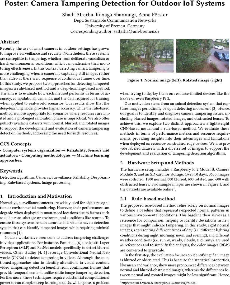
The experimental platform consists of a Raspberry Pi 2 Model B equipped with a Camera Module 3 and an SD card for storage. Over a ten‑day period, 3 600 images were collected in a real‑world outdoor setting: 1 800 normal images captured under varying lighting (night, morning, noon, evening) and weather (sunny, windy, cloudy, rainy) conditions, 600 blurred images, 600 rotated images, and 600 images with obstructed lenses. The authors make the full dataset publicly available via a university repository, providing a valuable resource for the community.

Rule‑Based Method
The rule‑based approach relies on eight carefully selected normal reference images that span the aforementioned illumination and weather variations. All images are converted to grayscale to simplify processing. The method proceeds in several stages:

1. Keypoint Matching – ORB (Oriented FAST and Rotated BRIEF) keypoints are extracted from both the test image and each reference image. A brute‑force matcher (BFMatcher) counts the number of “good” matches. If the count falls below a calibration‑derived threshold, the image is flagged as abnormal.

2. Blur Detection – For images already identified as potentially abnormal, a Laplacian operator computes the variance of the intensity values. A variance below a preset value indicates insufficient sharpness, and the image is classified as blurred.

3. Obstruction Detection – If the image is not blurred, the standard deviation of pixel intensities is evaluated. Very low deviation suggests a uniform or empty frame, which the authors interpret as a lens‑obstructed case.

4. Rotation Detection – When the match count exceeds the threshold, a homography matrix is estimated to recover the rotation angle. Angles greater than 50° trigger a “rotated” label; otherwise the image is considered normal.

Because this pipeline does not involve any learning phase, the model size is only 8.77 KB, and the average inference time per image is 0.07 seconds on the Raspberry Pi 2. The method achieves an overall accuracy of 90.5%, precision of 90.36%, recall of 90.66%, and an F1‑score of 90.51% on a balanced test set (50 % abnormal).

CNN‑Based Method
The deep‑learning solution is a relatively shallow CNN built with TensorFlow/Keras. Its architecture consists of three convolutional blocks (32, 64, and 128 filters respectively), each followed by ReLU activation and max‑pooling, a fully connected layer with 128 units, and a final sigmoid neuron for binary classification (normal vs. abnormal). The network is trained on 2 400 images (1 200 normal, 1 200 abnormal) using a standard training regime (Adam optimizer, batch size 32, ~50 epochs).

On the same balanced test set, the CNN attains 99.75% accuracy, 99.83% precision, 99.66% recall, and an F1‑score of 99.74%. The average processing time per image drops to 0.02 seconds, reflecting the efficiency of modern GPU‑accelerated inference. However, the trained model occupies 37.8 MB of storage, which exceeds the memory capacity of many low‑end edge devices and may require additional optimization (e.g., quantization, pruning) for deployment. Moreover, the method’s performance hinges on the availability of a representative training corpus; relocating the camera or encountering new environmental conditions would necessitate collecting and labeling a fresh dataset, incurring significant time and bandwidth costs.

Comparative Evaluation
Table 1 in the paper juxtaposes the two approaches across several dimensions: accuracy, precision, recall, F1‑score, number of training/reference samples, model size, and average inference time. The CNN clearly outperforms the rule‑based method in all classification metrics, but its larger footprint and dependence on a sizable labeled dataset limit its suitability for ultra‑low‑resource scenarios. Conversely, the rule‑based pipeline, despite lower classification performance, excels in environments where memory, storage, and power are at a premium, and where acquiring abnormal examples for training is impractical. The authors note that increasing the number of reference images could improve the rule‑based method’s robustness, suggesting a trade‑off between calibration effort and detection quality.

Conclusions and Future Work
The study demonstrates that both approaches have merit, with the choice dictated by deployment constraints. For battery‑operated, bandwidth‑limited camera traps that capture images only intermittently (e.g., wildlife monitoring), the rule‑based solution offers a viable, near‑zero‑training path. In contrast, installations that can afford periodic model updates and possess modest computational resources may benefit from the higher accuracy and adaptability of a CNN. The authors propose future research directions including:

• Development of a hybrid system that first applies lightweight rule‑based checks (e.g., blur detection) and then invokes a compact CNN only when necessary, thereby balancing accuracy and resource consumption.
• Exploration of model compression techniques (quantization, pruning, knowledge distillation) to shrink the CNN’s footprint for true microcontroller deployment.
• Expansion of the dataset to multiple geographic locations and camera models, enabling evaluation of cross‑domain generalization.

By releasing the labeled dataset and providing a clear performance benchmark, the paper contributes valuable resources to the emerging field of static‑image tampering detection for outdoor IoT camera networks.