Taking the GP Out of the Loop

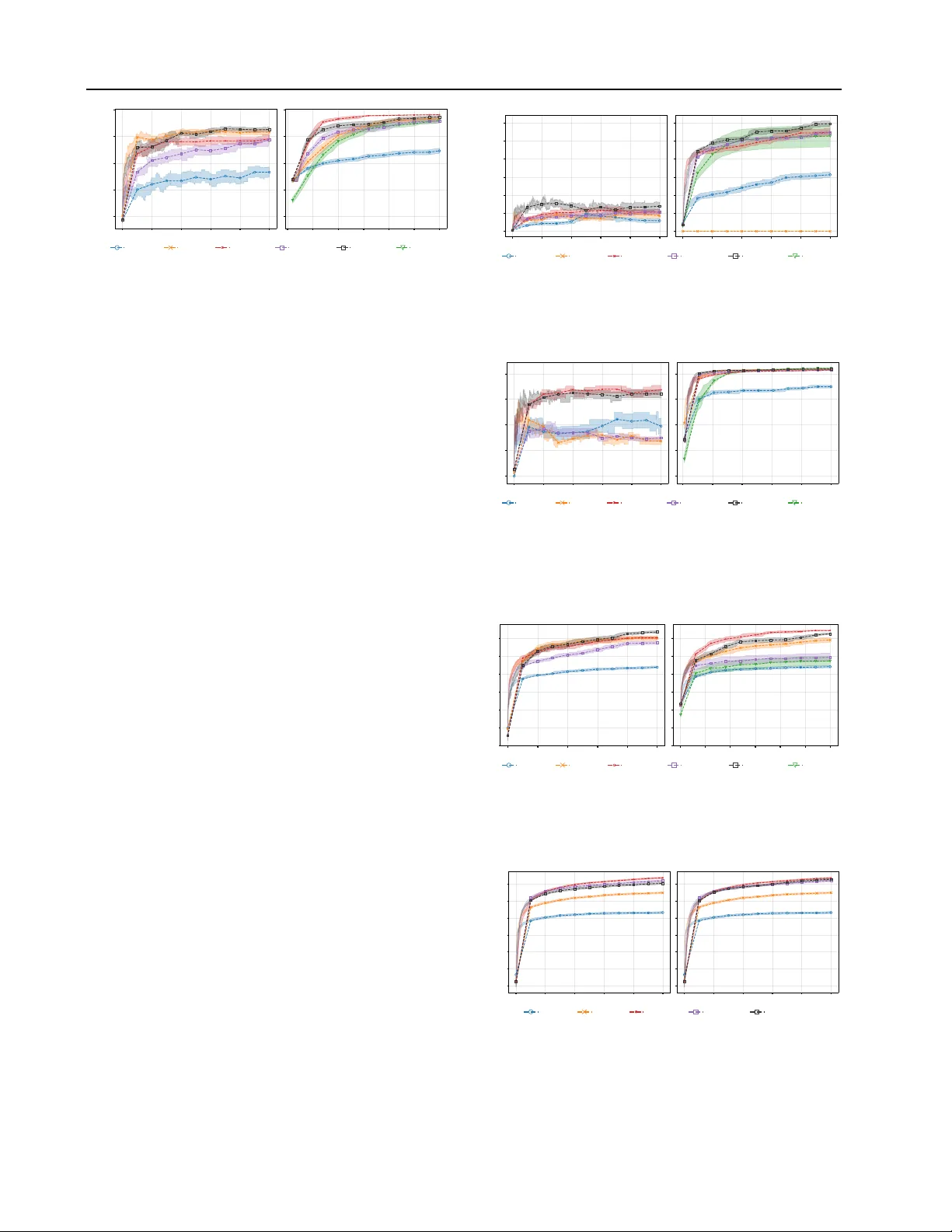
T aking the GP Out of the Loop Mehul Bafna 1 Siddhant Anand Jadha v 1 David Sweet 1 Abstract Bayesian optimization (BO) has traditionally solved black-box problems where function e valu- ation is e xpensiv e and, therefore, observations are few . Recently , howe ver , there has been growing interest in applying BO to problems where func- tion ev aluation is cheaper and observations are more plentiful. In this regime, scaling to many observations N is impeded by Gaussian-process (GP) surrogates: GP hyperparameter fitting scales as O ( N 3 ) (reduced to roughly O ( N 2 ) in modern implementations), and it is repeated at e very BO iteration. Man y methods impro ve scaling at acqui- sition time, but hyperparameter fitting still scales poorly , making it the bottleneck. W e propose Epis- temic Nearest Neighbors (ENN), a lightweight alternativ e to GPs that estimates function v alues and uncertainty (epistemic and aleatoric) from K -nearest-neighbor observations. ENN scales as O ( N ) for both fitting and acquisition. Our BO method, T uRBO-ENN, replaces the GP surrogate in T uRBO with ENN and its Thompson-sampling acquisition with UCB = µ ( x ) + σ ( x ) . For the special case of noise-free problems, we can omit fitting altogether by replacing UCB with a non- dominated sort ov er µ ( x ) and σ ( x ) . W e show empirically that TuRBO-ENN reduces proposal time (i.e., fitting time + acquisition time) by one to two orders of magnitude compared to T uRBO at up to 50,000 observations. 1. Introduction Bayesian optimization (BO) is commonly used in settings where e valuations are e xpensiv e, such as A/B testing (days to weeks) ( Quin et al. , 2023 ; Sweet , 2023 ), materials exper- iments (roughly 1 day) ( K otthoff et al. , 2021 ). It has also been applied to simulation optimization problems in engi- neering, logistics, medicine, and other domains ( Amaran 1 Department of Graduate Computer Science and Engineering, Y eshi va Uni versity , Ne w Y ork, NY 10033, USA. Correspondence to: David Sweet . Pr eprint. F ebruary 5, 2026. et al. , 2017 ). More recently , BO has been used in settings where ev aluations are fast and can be run in parallel—for example, lar ge-scale simulations in engineering design. In such cases, thousands of ev aluations may be generated dur- ing a single optimization run ( Daulton et al. , 2021 ). The proposal time for BO methods typically scales poorly with the number of observations, N , because proposals are generated by fitting and querying a Gaussian process (GP) surrogate. Modern, optimized implementations require O ( N 2 ) time per query . W e refer to problems with large N as Bayesian optimization with many observations (BOMO) , and present a method that reduces the proposal-time scaling to O ( N ) . It is important to distinguish between BOMO and BO with many design parameters – high-dimensional Bayesian op- timization (HDBO). Generally , we expect to need more observations to optimize more parameters since there are simply more possible designs to ev aluate. This e xpectation is codified, for example, in Ax’ s ( Meta , 2023 ) prescrip- tion to collect 2 × D observations before fitting a surrogate (where D is the number of design parameters, or dimen- sions ). Ho we ver , the number of observ ations necessary to locate a good design depends on aspects of a problem be- yond just D . For example, ( W ang et al. , 2016 ) optimizes a one-billion-parameter analytical function with only 500 observations, while ( Daulton et al. , 2021 ) tak es 1500 obser- vations to optimize a challenging simulation problem with only 12 parameters. This work focuses on BOMO. Specifically , we ask: Can we mak e a state-of-the-art BO algorithm significantly faster on BOMO pr oblems while pr oducing comparable- quality solutions? W e are concerned mainly with scaling (with N ) but we also report on w all time. Our approach is to strate gically simplify T uRBO ( Eriksson et al. , 2019b ), then compare solution quality , scaling, and running time. W e propose a nov el K -nearest neighbors surrogate, Epis- temic Nearest Neighbors (ENN), which estimates function values and uncertainty (both epistemic and aleatoric). W e integrate this approach into T uRBO ( Eriksson et al. , 2019b ) by replacing its GP surrogate and Thompson sampling ac- quisition method with ENN and UCB ( Srini v as et al. , 2010 ). Figure 1 shows that GP-based BO methods e xhibit approxi- 1 T aking the GP Out of the Loop mately O ( N 2 ) running time, whereas alternativ e-surrogate methods, such as T uRBO-ENN, scale as O ( N ) . In addi- tion to linear scaling, T uRBO-ENN achiev es much lower absolute proposal times than the other methods. Contributions This paper makes the follo wing contrib u- tions: • W e introduce Epistemic Nearest Neighbors (ENN) , a lightweight K -nearest-neighbor surrogate that es- timates both function value and uncertainty (epistemic and aleatoric) with O ( N ) fitting and querying time. • W e develop T uRBO-ENN , which replaces T uRBO’ s GP surrogate and Thompson sampling with ENN and UCB; for noise-free problems, we also describe a fitting-free v ariant based on non-dominated sorting ov er ( µ ( x ) , σ ( x )) . Proposal (fitting + acquisition) time is O ( N ) . • W e empirically e v aluate scaling and solution quality up to tens of thousands of observations in realistic simulation problems, showing one to two orders-of- magnitude reductions in proposal time while remaining competitiv e in optimization performance. • W e sho w that T uRBO-ENN is a Pseudo-Bayesian Opti- mization (PBO) method by verifying that its surrogate, uncertainty quantifier , and acquisition satisfy PBO con- ditions (Appendix A ), which guarantee con ver gence. 2. Background 2.1. Bayesian Optimization A Bayesian optimizer proposes a design, x ∈ [0 , 1] D , giv en some observ ations, D = { ( x i , y i ) } N i =1 , y i = f ( x i ) . A typical BO method consists of two components: a surrogate and an acquisition method. A surrogate is a model of f ( x ) mapping a design, x , to both an estimate of f ( x ) , µ ( x ) , and a measure of uncertainty in that esti- mate, σ ( x ) . An acquisition method determines the proposal, x p = arg max x α ( µ ( x ) , σ ( x )) , where the arg max is found by numerical optimization (e.g., via BFGS ( Meta , 2024a )) or by e valuating α ( · , · ) ov er a set of x samples, for example, uniform in [0 , 1] D or following any number of sampling schemes ( Kandasamy et al. , 2017 ; Eriksson et al. , 2019b ; Rashidi et al. , 2024 ). 2 . 1 . 1 . S U R R O G A T E The usual BO surrogate is a Gaussian process ( Rasmussen & W illiams , 2006 ). Gi ven observ ations D = { ( x i , y i ) } N i =1 , the GP posterior at a new point x has mean and variance 0 25 50 75 N 0 25 50 75 100 proposal time (s) (a) D = 100 0 100 200 N 0 5 10 15 (b) D = 300 0 250 500 750 N 0 10 20 30 proposal time (s) (c) D = 1000 0 250 500 750 N 0 . 2 0 . 3 0 . 4 0 . 5 (d) D = 1000, Zoom ucb:sparse ucb turbo-one vecchia optuna turbo-enn F igur e 1. Mean proposal time (in seconds) versus number of ob- servations ( N ) for sev eral Bayesian optimization methods. W e set N = D in these runs. Subfigures show results for (a) D = 100 , (b) D = 300 , (c) D = 1000 , and (d) a zoomed-in view of (c), av eraged over man y optimization runs (see Section 5 ). GP-based methods ( ucb and turbo-1 ) scale approximately as O ( N 2 ) , while optuna , which uses a P arzen estimator , vecchia , a nearest-neighbor GP method, and our method ( turbo-enn ) scale linearly in N . Scaling behavior for ucb:sparse , which uses a sparse GP , is not simple. Results are a veraged ov er 12 functions × 10 BO runs/function = 120 runs for each optimiza- tion method. The functions, { ackley , rastrigin , sphere , trid , booth , mccormick , dixonprice , rosenbrock , dejong5 , easom , branin , stybtang }, consist of two func- tions each from the six categories of optimizer test function in ( Surjanovic & Bingham , 2013 ). The various methods are dis- cussed in more detail in Section 3 . A ≡ K ( X, X ) + σ 2 0 I , (1) µ ( x ) = K ( X, x ) ⊤ A − 1 y , (2) σ 2 ( x ) = K ( x, x ) − K ( X, x ) ⊤ A − 1 K ( X, x ) . (3) where σ 0 is an inferred aleatoric uncertainty . The N × N kernel matrix, K ( X, X ) , has elements K ( X, X ) ij = k ( x i , x j ) , where k ( · , · ) is a kernel function, e.g., a squared exponential k ( x i , x j ) = exp  −∥ x i − x j ∥ 2 / (2 λ )  , although others are common, too ( Rasmussen & W illiams , 2006 ). Similarly , the kernel vec- tor K ( X, x ) ∈ R N has entries K ( X, x ) i = k ( x i , x ) . The kernel matrix is the pairwise co variance between all obser - vations, and the k ernel vector is the cov ariance between the query point x and the observations. Constructing the N × N kernel matrix K ( X, X ) takes N ( N − 1) / 2 ev aluations of k ( · , · ) , which is O ( N 2 ) . Exact GP training then requires solving linear systems in v olving K ( X, X ) (typically via a Cholesky factorization), which is 2 T aking the GP Out of the Loop O ( N 3 ) in general; modern iterati ve solvers can reduce k ey GP computations to roughly O ( N 2 ) ( Gardner et al. , 2018 ). Hyperparameter fitting The hyperparameters, λ and σ 0 , the kernel length-scale and noise lev el, are typically chosen to maximize the mar ginal log-lik elihood of the observ ations, D , by a numerical optimizer such as SGD ( Eriksson et al. , 2019b ) or BFGS ( Meta , 2024a ). When optimizing, one needs to reconstruct K for each hyperparameter proposed by the optimizer . 2 . 1 . 2 . A C Q U I S I T I O N M E T H O D There are many acquisition methods in the literature. Three common ones are: Upper Confidence Bound (UCB) x p = arg max x  µ ( x ) + β σ ( x )  , where β is a constant. The first term encourages exploitation of D , i.e. biasing x p tow ards a design that is expected to work well, while the second term encourages exploration of the design space so as to collect new observa- tions that will improv e future surrogates. Expected Impro vement (EI) x p = arg max x E [max { 0 , y ( x ) − y ∗ } ] , where y ∗ = max y m , and the expectation is taken o ver y ( x ) ∼ N ( µ ( x ) , σ 2 ( x )) . Thompson Sampling (TS) x p = arg max x y ( x ) , where y ( x ) is a joint sample from the GP at a set of x values ( Kandasamy et al. , 2017 ). (A joint sample modifies equa- tions equation 3 to account for the cov ariance between each x that is being sampled.) 3. Related W ork Approaches to scaling BO to many observations include acceleration of exact GP computations, trust regions, and various alternati ve surrog ates. Our method combines a trust region with a no vel alternati ve surrogate, ENN. W e briefly revie w v arious approaches below . Blackbox Matrix-Matrix Multiplication A conjugate- gradient algorithm replaces the in version of K ( X, X ) in equation equation 3 with a sequence of matrix multiplies, re- ducing the hyperparameter-fitting time comple xity of a GP from O ( N 3 ) to O ( N 2 ) ( Gardner et al. , 2018 ). A Lanczos algorithm can speed up GP posterior sampling (e.g., used in Thompson sampling) to constant-in- N ( Pleiss et al. , 2018 ). T rust Region BO The T uRBO algorithm ( Eriksson et al. , 2019b ) reduces wall-clock time in two ways: (i) It occasion- ally restarts, discarding all pre vious observations, resetting N to 0. (ii) It restricts Thompson samples to within a trust region, a small subset of the overall design space where good designs are most likely , thus a voiding needless ev alua- tions else where. Our method replaces the GP surrogate in T uRBO with ENN. Sparsity Sparse GP methods ( T itsias , 2009 ) replace obser - vations in the co variance matrix with M summary (induc- ing) points, reducing the training comple xity of GP fitting to O ( N M 2 ) and inference to O ( N M ) . Optimally , M in- creases only slowly with N ( Burt et al. , 2020 ), although the recommended setting for a popular BO library ( Meta , 2024a ) is M = 0 . 25 N , which results in O ( N 2 ) inference. Fitting requires choosing inducing points (various approaches exist ( Moss et al. , 2023 )) and can be computationally intensiv e, since the variational loss is more complex than the e xact GP likelihood. Figure 1 shows a sparse GP-based method displaying a complex proposal time beha vior with N . Modeling p ∗ ( x ) An open-source optimizer , Optuna ( Akiba et al. , 2019 ; Optuna , 2025 ), does not model f ( x ) . Instead, it models p ∗ ( x ) = P { x = arg max x f ( x ) } . The model is a Parzen estimator , a linear combination of functions of the observations, which has O ( N ) query time. Optuna uses a modified EI-based acquisition method ( W atanabe , 2023 ). Parametric surr ogates Other methods of scaling to lar ge N replace the GP with a neural network ( Snoek et al. , 2015 ) or a random forest ( Hutter et al. , 2011 ). While fitting a neural network or random forest scales as O ( N ) , the fitting processes are complex and introduce man y tunable hyper- parameters. Query time depends on the model architecture and is independent of N . Due to the fitting comple xity , we do not compare to these methods in this paper . Nearest-neighbors V ecchia GP methods ( Jimenez & Katz- fuss , 2022 ; Jimenez , 2025 ) and others ( Gramac y & Apley , 2015 ; W u et al. , 2024 ) condition GP inference only on M nearest neighbors. Fitting and inference scale as O ( N M ) . One V ecchia GP-based optimization method explored in ( Jimenez & Katzfuss , 2022 ) combines nearest-neighbor lookups with T uRBO’ s trust region sampling. Our approach is similar in that it uses nearest-neighbor lookups and a trust region, b ut our ENN estimates are constructed from simpler linear combinations of observations (see 4 ), resulting in a significant speedup, see Figure 1 . Note that none of the alternativ e (non-GP) surrogates dis- cussed abov e, except for ENN, support principled uncer- tainty quantification. Chen & Lam ( 2025 ) recently introduced Pseudo-Bayesian Optimization (PBO) , which establishes con vergence guar - antees for any method whose surrogate, uncertainty quanti- fier , and acquisition satisfy certain conditions. Appendix A shows that T uRBO-ENN satisfies these conditions and, therefore, qualifies as a PBO method, inheriting the associ- ated con ver gence guarantees. 3 T aking the GP Out of the Loop 4. Epistemic Nearest Neighbors 4.1. ENN Surrogate A surrogate maps designs or parameters, x , to measure- ments, y = f ( x ) + sε , where s is the aleatoric uncertainty in y . A triple, ( x, y , s ) is called an observ ation. A data set, D is a collection of observations, ( x m , y m , s m ) ∈ D . W e define our ENN surrog ate by four properties. For a query point, x , giv en D , • Independence : Each observ ation, ( x m , y m , s m ) ∈ D is an independent estimate of f ( x ) . • Conditional mean : µ ( x | x m , y m , s m ) = y m . • Conditional aleatoric variance : σ 2 a ( x | x m , y m , s m ) = s 2 0 + s 2 m • Conditional epistemic variance : σ 2 e ( x | x m , y m , s m ) = c e d 2 ( x, x m ) where d ( x, x m ) denotes the (Euclidean) distance from x to x m , and s 0 and c e are hyperparameters. Precisely speaking, we treat the estimates as independent for tractability . Equating epistemic variance to squared distance from the measurement, x m , captures the intuition that similar designs will hav e similar ev aluations, f ( x ) . Combining estimates For a query point, x , we com- bine the mean estimates from each of its K nearest neigh- bors using the linear combination with minimum v ariance, the precision-weighted av erage ( Cochran , 1954 ). Defining σ 2 ( x | x i , y i , s i ) = σ 2 a ( x | x i , y i , s i ) + σ 2 e ( x | x i , y i , s i ) , we write µ ( x ) = P K i σ − 2 ( x | x i , y i , s i ) µ ( x | x i , y i , s i ) P K i σ − 2 ( x | x i , y i , s i ) and similarly for the aleatoric variance σ 2 a ( x ) = P K i σ − 2 ( x | x i , y i , s i ) σ 2 a ( x | x i , y i , s i ) P K i σ − 2 ( x | x i , y i , s i ) Finally , we estimate epistemic variance of µ ( x ) : σ 2 e ( x ) = V ar[ µ ( x )] = 1 P K i σ − 2 ( x | x i , y i , s i ) Computational cost Finding the K nearest neighbors requires e valuating d ( x, x i ) for all N observat ions, at a cost of O ( N ln K ) time per query (using a max heap ( Cormen et al. , 2009 )). T reating the observ ations as independent relie ves us from calculating the O ( N 2 ) pairwise covariances between observ ations as in the calculation of K ( x m , x ) in equations 3 . Our implementation uses the Python module Faiss ( Meta , 2024b ) to find the K nearest neighbors. Hyperparameters The hyperparameters s 0 and c e are fit by T ype-II MLE optimization of an LOOCV [leave-one-out cross v alidation ( Hastie et al. , 2009 )] average pseudolik eli- hood ( Rasmussen & W illiams , 2006 ). log L ( θ ) = 1 N N X n =1 ℓ − n ( θ ) where θ = { s 0 , c e } ,and ℓ − n ( θ ) = − 1 2  log(2 π σ − n ( x n ; θ ) 2 ) + ( y n − µ − n ( x n ; θ )) 2 σ − n ( x n ; θ ) 2  . where ( µ − n ( x n ; θ ) , σ − n ( x n ; θ )) are LOO ENN estimates. Each LOO estimate takes O ( N ln K ) time. F orming N of them would, thus, tak e O ( N 2 ln K ) . T o a void introducing an ∼ N 2 computation, we approximate the average pseudo- likelihood with a fixed-size, P , subsample ( S P ) of the N observations. [ log L ( θ ) = 1 P X n ∈ S P ℓ − n ( θ ) . T o calculate [ log L ( θ ) we need to produce LOO ENN esti- mates for P points, taking only O ( P N ln K ) calculations. W e justify a constant P by noting that we only require our likelihood estimate to be precise enough to support a decision about which hyperparameters to use. If the variance V ar[ ℓ n ( θ )] = σ 2 ℓ ( θ ) , then V ar h [ log L ( θ ) i = 1 P σ 2 ℓ ( θ ) . Hence, fixing P fixes the precision (in verse v ariance) of the likelihood estimate (independently of N ). T o further limit the amount of computation dev oted to hy- perparameter tuning, we fix K to a single v alue for the entirety of all BO runs. W e find that K = 10 giv es good performance and leav e it fixed there throughout this paper . Figure 2 depicts the ENN surrogate for f ( x ) = sin(2 π x ) with various noise le vels. Note that, in general, the ENN estimate (dashed line) may or may not pass through an observation. In particular, the three right-most observ ations all ha ve the same x value but dif ferent y v alues due to noise, yet ENN provides a single mean estimate at that x value; ENN is an estimator , not an interpolator . 4.2. Acquisition W e follow a modified version of the acquisition method of T uRBO ( Eriksson et al. , 2019b ). Candidate generation is the same in both cases: we center a trust re gion T ⊆ [0 , 1] D 4 T aking the GP Out of the Loop 0 . 00 0 . 25 0 . 50 0 . 75 1 . 00 x − 4 − 2 0 2 4 y N = 10, σ ε = 0.0 0 . 00 0 . 25 0 . 50 0 . 75 1 . 00 x N = 10, σ ε = 0.3 F igur e 2. Epistemic nearest neighbors (ENN) surrogate for two noise lev els, σ ε . The dashed line shows µ ( x ) and the shaded region is ± 2 σ ( x ) . The solid red line is the function being estimated, f ( x ) = sin(2 π x ) . at an incumbent point x 0 , then generate many candidates { x c } ⊂ T via RAASP sampling ( Rashidi et al. , 2024 ). The dif ference is how we (i) choose the incumbent and (ii) choose the next arm from the candidates. Noise-free acquisition • Incumbent : set x 0 ∈ arg max x ∈{ x 1 ,...,x N } y ( x ) . • Arm selection : Compute ( µ ( x c ) , σ ( x c )) for candi- dates and run a non-dominated sort (NDS) ( Buzdalo v & Shalyto , 2014 ; De Ath et al. , 2021 ) ov er the two objectiv es µ ( x c ) and σ ( x c ) . NDS produces a Pareto front of candidates, from which we randomly sample the proposed arm, x arm . This dif fers from the original T uRBO, which selects x arm via Thompson sampling: x arm = arg max x c { y ( x c ) } where { y ( x c ) } is a joint GP sample ov er the candidates. For noise-free problems (common in simulation ( Santner et al. , 2019 )), we omit hyperparameter fitting altogether , as ENN hyperparameter fitting only serves to calibrate un- certainty to match µ ( x ) (i.e., to determine c e ) and to infer the noise lev el (which is known, a priori , for noise-free problems, to be s 0 = 0 ). But NDS ne ver directly compares σ ( x ) to µ ( x ) . All comparisons in the sort are among σ ( x ) values or among µ ( x ) values separately ( Buzdalov & Sha- lyto , 2014 ). Thus, fitting the hyperparameters for noise-free problems at best wastes compute time, and, at worst risks introducing hyperparameter estimation error (i.e., setting s 0  = 0 ). Noisy acquisition • Fit : Fit ENN hyperparameters ( s 0 , c e ) by maximiz- ing the subsampled LOO pseudolikelihood [ log L ( θ ) (Section 4 ). • Incumbent : Eriksson et al. ( 2019b ) recommends se- lecting the maximizer of the denoised observations, x 0 = x arg max i µ ( x i ) . W e avoid computing µ ( x i ) for Algorithm 1 T uRBO-ENN with two acquisition variants: noise-free (ENN+NDS, no fitting) and noisy (fit ENN + UCB) 1: Input: objectiv e f : [0 , 1] D → R ; rounds R ; K ; P ; noise_free (bool); trust region lengthscale, ℓ 2: Initialize: LHD sample { x i } N init i =1 , e valuate y i = f ( x i ) , set D ← { ( x i , y i ) } ; initialize trust region T 3: f or t = 1 to R do 4: if noise_free then 5: s 0 ← 0 , c e ← 1 6: else 7: ( s 0 , c e ) ← arg max s 0 ,c e LOOCV P ( s 0 , c e ) 8: end if 9: if noise_free then 10: x 0 ← x arg max i y i 11: else 12: I top ← topK( { y i } ; K ) 13: x 0 ← x arg max i ∈ I top µ ( x i ) 14: end if 15: T ← T ( x 0 , ℓ ) 16: { x c } ← RAASP( T ) 17: ( µ c , σ c ) ← ENN( { x c } ; D , s 0 , c e ) 18: if noise_free then 19: x arm ∼ F ront 1 (NDS( { x c } ; µ c , σ c )) 20: else 21: x arm ← arg max x c  µ c + σ c  22: end if 23: Evaluate y arm ← f ( x arm ) and append ( x arm , y arm ) to D 24: ℓ ← up date( ℓ ) 25: end f or 26: Output: x best ∈ arg max ( x i ,y i ) ∈D y i all N observations since that would tak e O ( N 2 ln K ) time. Instead, we first subset to the top- K observed y i , then set x 0 = x arg max i ∈ I top µ ( x i ) where I top are the indices of those top- K observ ations. • Arm selection : Compute ( µ ( x c ) , σ ( x c )) for candi- dates and select x arm = arg max x c U C B ( x c ) where U C B ( x ) = µ ( x ) + σ ( x ) (we take β = 1 ). Algorithm 1 summarizes both variants. An implementation of T uRBO-ENN, along with the original T uRBO, is a vail- able in the pip -installable Python library , with source and examples on GitHub at . For the exact, original specifications of T ← T ( x 0 , ℓ ) , RAASP( T ) and ℓ ← up date( ℓ ) , please see ( Eriksson et al. , 2019b ; a ). 5 T aking the GP Out of the Loop 5. Numerical Experiments W e benchmark T uRBO - ENN by optimizing fi ve noisy simu- lations both with natural and fr ozen noise, which we define subsequently (section 5.1 ). LunarLander -v3 A 2D physics simulation ( Farama , 2024 ) where the goal is to safely land a spacecraft at a designated stop using continuous engine thrusters while managing fuel consumption and orientation. The controller is the 12D heuristic, non-differentiable controller presented in ( Eriksson et al. , 2019b ). The simulators for this task and the next two are implemented in the Gymnasium (fmr . OpenAI gym) Python package ( Brockman et al. , 2016 ). Hopper -v5 A 2D physics simulation ( Farama , 2024 ) where the goal is to safely hop a one-legged robot forw ard. The controller is a 34D linear mapping from states to actions with hard clamping of action v alues, similar to ( Mania et al. , 2018 ). BipedalW alker-v3 A 2D physics simulation ( F arama , 2024 ) where the goal is to navigate across randomly gener - ated rough terrain using a two-le gged robot. The controller is a 16D heuristic, non-differentiable controller designed interactiv ely with Cursor ( Cursor ), GPT -5.2 ( OpenAI ), and Claude Opus 4.5 ( Anthropic ). Code for this controller is av ailable at . Push-v5 A 2D physics simulation where the goal is to push two objects using two robot hands. The controller is the 14D heuristic, non-differentiable controller studied in ( W ang et al. , 2018 ) and ( Eriksson et al. , 2019b ). LASSO-DNA A 180D hyperparameter optimization (HPO) problem from LASSOBench ( Šehi ´ c et al. , 2022 ). The objective is to minimize a validation error ov er 180 LASSO weights. This HPO problem is similar to a sim- ulation optimization problems in that the ev aluation time is short and many observations may be needed to find an acceptable solution. In ( Šehi ´ c et al. , 2022 ), T uRBO ga ve the best performance of the optimizers tested on this problem. (NB: W e treat this as a maximization problem by flipping the sign of the objectiv e.) Across all tasks, T uRBO - ENN attains objectiv e values com- parable to T uRBO while reducing proposal time by one to two orders of magnitude, with greater reductions for lar ger N . W e also compare to Optuna ( Akiba et al. , 2019 ), another O ( N ) optimizer , and CMA-ES ( Hansen , 2023 ), an O (1) ev olution strategy optimizer . Note that CMA-ES requires num_arms > 1 and, thus, is omitted from sequential runs (i.e., where num_arms=1 ). Optuna exhausted our com- pute budget (5 hours) on Hopper-v5 with frozen noise, so we did not include it in that experiment. 5.1. Noise Handling The simulators are driven, in part, by a seeded random number generator such that multiple runs with the same controller and different seed v alues will produce different episode returns (i.e., the objecti ve v alues). W e take two ap- proaches to handling noise, natural and frozen, and produce comparisons for each. 5 . 1 . 1 . N AT U R A L N O I S E Natural noise models a setting where one cannot control the noise source with a seed. Some simulation en vironments might be unav oidably non-deterministic ( Isaac Lab Project Dev elopers ), and, of course, any physical system would produce uncontrolled noise. For this style, we use a different seed for every episode of the simulator throughout the entire optimization run. W e reproduce the same seed sequence for each optimization method to make their runs more comparable. Thus, to a sin- gle optimizer , the simulator looks noisy , yet each optimizer sees the same noise. T o ev aluate an optimizer , at each round we ask it for its pick of a "best" parameter setting. W ith that setting, we simulate sev eral (e.g., 10) times with a fix ed set of ev aluation seeds (distinct from the seeds used during optimization) and record the mean episode return, r passive . The intention of r passive is to estimate the expected episode return we would achieve were we to stop the optimizer and accept its best parameter setting for future, prolonged use of the controller . Note that the optimizer’ s pick of "best setting" is sensitiv e to noise and may not yield the best expected future episode return. Thus, the natural-noise plots are not generally monotonically increasing. Note that the optimizer ne ver sees r passive . In our figures, the number of passiv e ev aluation seeds used to compute r passive is num_denoise_passive . T o pick the best parameter setting, ( Eriksson et al. , 2019b ) recommends selecting the observ ation, ( x i , y i ) , with the largest µ ( x i ) value, as gi ven by the surrogate. W e follow this approach for T uRBO, but modify it for T uRBO-ENN. In the latter case, we first subset to the top K observations by y i , then find arg max i µ ( x i ) of this K -sized set. Preprocessing by subsetting reduces the time scaling of picking the max from O ( N 2 ln K ) to O ( N K ln K ) . 5 . 1 . 2 . F R O Z E N N O I S E Frozen noise ( Kim et al. , 2003 ) con v erts a noisy simulator into a noise-free objective function. T o implement frozen noise, we produce a fix ed set, S , of seeds at the outset of the optimization run. T o e valuate a design, we run the simulator onces for each seed in S and return to the optimizer the mean episode return ov er all seeds. Noise-free problems tend to be easier to solve, as we’ll see in the figures below , and is 6 T aking the GP Out of the Loop 0 2000 4000 6000 8000 10000 N − 100 0 100 200 300 y best 0 250 500 750 1000 1250 1500 N random optuna turbo-one turbo-zero turbo-enn cma F igur e 3. LunarLander-v3, D = 12 , using the controller presented in ( Eriksson et al. , 2019b ). Left: Natural noise. num_arms = 1, num_denoise_passive = 30. Right: Frozen noise. num_arms = 50, num_denoise_obs = 50. an approach commonly employed in BO and RL literature ( Kim et al. , 2003 ; Eriksson et al. , 2019b ; Salimans et al. , 2017 ; Schulman et al. , 2017 ). In our figures, the number of seeds in the seed set is named num_denoise_obs . 5.2. Results W e label our method turbo-enn ; it uses the noisy ENN+UCB variant for natural-noise experiments and the noise-free ENN+NDS variant for frozen-noise experiments. W e label the original T uRBO turbo-one (one trust re- gion). W e include an ablation, turbo-zero , which pro- poses arms by uniformly sampling from T uRBO’ s RAASP candidate set without a surrogate. W e also compare to Op- tuna ( optuna ), CMA-ES ( cma ), and a random baseline that samples arms uniformly in [0 , 1] D . W e repeat each optimization run 30 times with dif ferent seed sets and plot the mean ± two standard errors. In each case, we see turbo-enn producing designs of similar quality to those produced by turbo-1 but with one to two orders of magnitude smaller proposal times. T otal proposal times are listed in T able 1 . The notation y best indicates either the mean objecti ve v alue on the e valuation seed set (for natural noise, left subplots) or the best objective val ue observed so far (for frozen noise). N is the number of observations collected so f ar . Our experiments include runs as large as N = 50 , 000 observ ations. Natural noise is generally more difficult for all algorithms than frozen noise. Speedup, the ratio of the proposal time of turbo-one to the proposal time of turbo-enn , ranges from 12.1 to 150.7. Speedup is problem-dependent, but it is generally lar ger for larger N and for frozen noise. Note that the frozen noise algorithm omits hyperparameter fitting, reducing computation time. The surrogate-free algorithm turbo-zero performs well on frozen-noise problems but is rarely the best, and it suffers on natural-noise problems. 0 2000 4000 6000 8000 10000 N 0 250 500 750 1000 1250 1500 y best 0 10000 20000 30000 40000 50000 N random optuna turbo-one turb o-zero turb o-enn cma F igur e 4. Hopper-v5, D = 34 , using a linear controller, sim- ilar to ( Mania et al. , 2018 ). Left: Natural noise. num_arms = 1, num_denoise_passive = 10. Right: Frozen noise. num_arms = 50, num_denoise_obs = 10. 0 2000 4000 6000 8000 10000 N − 100 0 100 200 300 y best 0 1000 2000 3000 4000 5000 N random optuna turbo-one turbo-zero turbo-enn cma F igur e 5. BipedalW alk er-v3, D = 16 , using a heuristic con- troller designed interactiv ely with Cursor ( Cursor ), GPT -5.2 ( Ope- nAI ), and Claude Opus 4.5 ( Anthropic ). Left: Natural noise. num_arms = 1, num_denoise_passive = 10. Right: Frozen noise. num_arms = 50, num_denoise_obs = 10. 0 2000 4000 6000 8000 10000 N − 2 0 2 4 6 8 10 y best 0 2500 5000 7500 10000 12500 15000 N random optuna turbo-one turbo-zero turb o-enn cma F igur e 6. Push-v5, D = 14 , using a heuristic controller presented in ( W ang et al. , 2018 ) and ( Eriksson et al. , 2019b ). Left: Natural noise. num_arms = 1, num_denoise_passive = 30. Right: Frozen noise. num_arms = 50, num_denoise_obs = 50. 0 200 400 600 800 1000 N − 0 . 42 − 0 . 40 − 0 . 38 − 0 . 36 − 0 . 34 − 0 . 32 − 0 . 30 y best 0 200 400 600 800 1000 N random optuna turbo-one turbo-zero turbo-enn F igur e 7. LASSO-DN A, D = 180 , a weighted-LASSO hy- perparameter optimization problem from LASSOBench ( Še- hi ´ c et al. , 2022 ). Left: Natural noise. num_arms = 1, num_denoise_passive = 10. Right: Frozen noise. num_arms = 1, num_denoise_obs = 10. 7 T aking the GP Out of the Loop T able 1. T otal proposal time (seconds) for each optimization method, summed over the full optimization run, for natural-noise (left subplots) and frozen-noise (right subplots) e xperiments. Dashes indicate that the method was not run for that setting. Speedup is computed as the ratio of the proposal time of turbo-one to the proposal time of turbo-enn . T ask D N Noise random cma turbo-zero optuna turbo-one turbo-enn speedup LunarLander-v3 12 300 natural <0.1 – 0.4 12.0 83.6 6.9 12 1500 frozen <0.1 0.1 0.1 115.6 52.2 0.6 89 Hopper-v5 34 10000 natural 0.7 – 52.6 8995.0 17582.5 822.8 21 50000 frozen 1.3 7.0 7.8 – 5532.4 41.2 134 BipedalW alker -v3 16 10000 natural 1.9 – 25.9 4373.0 3048.0 311.1 10 5000 frozen 0.3 0.8 0.7 1142.4 173.1 2.2 80 Push-v5 14 10000 natural 0.2 – 14.9 3485.9 3050.0 309.9 10 15000 frozen 0.1 1.3 7.9 11117.4 873.8 5.8 150 LASSO-DNA 180 1000 natural 0.1 – 41.2 910.0 6508.1 108.1 60 1000 frozen 0.1 – 40.0 915.3 6596.4 88.4 75 6. Limitations and Future W ork Improving scaling from O ( N 2 ) to O ( N ) enables BO to han- dle many more observations. W e wonder whether scaling could be improved ev en further in a BO, surrogate-based optimization algorithm. Perhaps ENN could be adapted to an approximate nearest neighbor algorithm ( Malkov & Y ashunin , 2020 ) that scales as O (ln N ) . W e note that the surrogate-free, sampling-only algorithm CMA-ES is con- stant in N , i.e. O (1) , and performs very well. The same holds true for our surrogate-free ablation, turbo-0 , and we think more attention to the sampling phase of BO may be beneficial. In this paper we use a constant v alue of K . Future w ork might explore w ays to choose a v alue of K appropriate to a particular problem or e ven to a particular observ ation set. Perhaps K could be tuned along with s 0 and c e . The original T uRBO uses Thompson sampling, an acquisi- tion method that enjoys near-optimal regret for multi-armed bandits ( Agrawal & Goyal , 2012 ) and works very well in Bayesian optimization ( Kandasamy et al. , 2018 ; Sweet , 2024 ). T o create a Thompson sample, the surrog ate needs to support joint sampling, b ut ENN does not yet support this. This could be an interesting av enue for future research. In GP surrogates, one lengthscale h yperparameter may be assigned to each dimension, a technique called automatic relev ance determination (ARD) ( W illiams & Rasmussen , 1995 ). Analogous techniques exist for nearest-neighbor models ( Li et al. , 2015 ). It may be fruitful to seek a fast, scalable method of weighting dimensions in ENN’ s distance metric. As D increases, Euclidean distance (to a query point) will discriminate less between observations, yet RAASP and the trust region may serve to ameliorate this problem. This is an interesting research question. Scientific and engineering simulations may contain parame- ter constraints, outcome (metric) constraints, mix ed v ariable types (e.g, continuous, ordinal, categorical), and multiple metrics. These are all aspects of optimization to which ENN should be adapted. While there is a con vergence guarantee, we provide no regret bounds. 7. Conclusion Bayesian optimization with many observations (BOMO) is an increasingly important setting, driv en by fast simula- tions and parallel ev aluation, where proposal time becomes significant relati ve to e valuation time. W e proposed T uRBO- ENN, a trust-region Bayesian optimization method that re- places the Gaussian-process surrogate in T uRBO with Epis- temic Nearest Neighbors (ENN), a lightweight K -nearest- neighbor surrogate that provides both a mean predictor and an uncertainty estimate with linear scaling in N under our implementation. For noisy objectiv es, T uRBO-ENN fits ENN hyperparameters and selects candidates using UCB. For deterministic objectives, it admits a fitting-free vari- ant that selects candidates via non-dominated sorting ov er ( µ, σ ) , further decreasing proposal time. Across the bench- marks we study , including runs with up to N = 50 , 000 observations, T uRBO-ENN achie ves solution quality com- parable to T uRBO while reducing proposal time by one to two orders of magnitude, with impro vements that gro w with N . Finally , we show in Appendix A that T uRBO-ENN sat- isfies the Pseudo-Bayesian Optimization axioms, providing a con ver gence guarantee. References Agrawal, S. and Goyal, N. Further optimal regret bounds for thompson sampling, 2012. URL https://arxiv. org/abs/1209.3353 . Akiba, T ., Sano, S., Y anase, T ., Ohta, T ., and K oyama, M. Optuna: A next-generation hy- perparameter optimization framew ork. Pr oceed- ings of the 25th ACM SIGKDD International Con- fer ence on Knowledge Discovery & Data Mining , 8 T aking the GP Out of the Loop 2019. URL https://api.semanticscholar. org/CorpusID:196194314 . Amaran, S., Sahinidis, N. V ., Sharda, B., and Bury , S. J. Simulation optimization: A re view of algorithms and applications. CoRR , abs/1706.08591, 2017. URL http: //arxiv.org/abs/1706.08591 . Anthropic. Claude opus 4.5. https://www. anthropic.com/ . Accessed 2026-01-23. Brockman, G., Cheung, V ., Pettersson, L., Schneider , J., Schulman, J., T ang, J., and Zaremba, W . Openai gym. CoRR , abs/1606.01540, 2016. URL http://arxiv. org/abs/1606.01540 . Burt, D. R., Rasmussen, C. E., and v an der W ilk, M. Con- ver gence of sparse variational inference in gaussian pro- cesses regression. Journal of Machine Learning Re- sear ch , 21(131):1–63, 2020. URL http://jmlr. org/papers/v21/19- 1015.html . Buzdalov , M. and Shalyto, A. A prov ably asymptotically fast v ersion of the generalized jensen algorithm for non- dominated sorting. In Bartz-Beielstein, T ., Branke, J., Filipi ˇ c, B., and Smith, J. (eds.), P arallel Pr oblem Solving fr om Natur e – PPSN XIII , pp. 528–537, Cham, 2014. Springer International Publishing. ISBN 978-3-319- 10762-2. Chen, H. and Lam, H. Pseudo-bayesian optimization, 2025. URL . Cochran, W . G. The combination of estimates from dif ferent experiments. Biometrics , 10(1):101–129, 1954. ISSN 0006341X, 15410420. URL http://www.jstor. org/stable/3001666 . Cormen, T . H., Leiserson, C. E., Rivest, R. L., and Stein, C. Intr oduction to Algorithms . MIT Press, Cambridge, MA, 3 edition, 2009. Cursor. Cursor . https://www.cursor.com/ . Ac- cessed 2026-01-23. Daulton, S., Eriksson, D., Balandat, M., and Bakshy , E. Multi-objectiv e bayesian optimization o ver high- dimensional search spaces. CoRR , abs/2109.10964, 2021. URL . De Ath, G., Everson, R. M., Rahat, A. A. M., and Fieldsend, J. E. Greed is good: Exploration and e xploitation trade- offs in bayesian optimisation. A CM T rans. Evol. Learn. Optim. , 1(1), April 2021. doi: 10.1145/3425501. URL https://doi.org/10.1145/3425501 . Eriksson, D., Pearce, M., Gardner, J., T urner , R. D., and Poloczek, M. T urbo: T rust region bayesian op- timization, 2019a. URL https://github.com/ uber- research/TuRBO . GitHub repository . Eriksson, D., Pearce, M., Gardner , J. R., T urner , R., and Poloczek, M. Scalable global optimization via local bayesian optimization. CoRR , abs/1910.01739, 2019b. URL . Farama. Gymnasium, 2024. URL https:// gymnasium.farama.org/index.html . Gardner , J. R., Pleiss, G., Bindel, D., W einberger , K. Q., and W ilson, A. G. Gpytorch: blackbox matrix-matrix gaussian process inference with gpu acceleration. In Pr oceedings of the 32nd International Confer ence on Neural Information Pr ocessing Systems , NIPS’18, pp. 7587–7597, Red Hook, NY , USA, 2018. Curran Asso- ciates Inc. Gramacy , R. B. and Apley , D. W . Local gaus- sian process approximation for large computer experi- ments. J ournal of Computational and Graphical Statis- tics , 24(2):561–578, 2015. doi: 10.1080/10618600. 2014.914442. URL https://doi.org/10.1080/ 10618600.2014.914442 . Hansen, N. The cma ev olution strategy: A tutorial, 2023. URL . Hastie, T ., Tibshirani, R., and Friedman, J. The Elements of Statistical Learning: Data Mining, Infer ence, and Pr e- diction . Springer Science & Business Media, New Y ork, NY , 2nd edition, 2009. ISBN 978-0387848570. Hutter , F ., Hoos, H. H., and Leyton-Bro wn, K. Sequential model-based optimization for general algorithm configu- ration. In Coello, C. A. C. (ed.), Learning and Intelligent Optimization , pp. 507–523, Berlin, Heidelber g, 2011. Springer Berlin Heidelberg. ISBN 978-3-642-25566-3. Isaac Lab Project Dev elopers. Reproducibility and determinism. https://isaac- sim.github. io/IsaacLab/main/source/features/ reproducibility.html . Last updated Jan 22, 2026. Accessed 2026-01-23. Jimenez, F . V ecchiabo, 2025. URL https://github. com/feji3769/VecchiaBO . Jimenez, F . and Katzfuss, M. Scalable bayesian opti- mization using vecchia approximations of gaussian pro- cesses, 2022. URL 2203.01459 . Kandasamy , K., Krishnamurthy , A., Schneider , J., and Poczos, B. Asynchronous parallel bayesian optimi- sation via thompson sampling, 2017. URL https: //arxiv.org/abs/1705.09236 . Kandasamy , K., Krishnamurthy , A., Schneider , J., and Poczos, B. Parallelised bayesian optimisation via 9 T aking the GP Out of the Loop thompson sampling. In Storkey , A. and Perez-Cruz, F . (eds.), Pr oceedings of the T wenty-F irst Interna- tional Confer ence on Artificial Intelligence and Statis- tics , volume 84 of Proceedings of Machine Learn- ing Resear ch , pp. 133–142. PMLR, 09–11 Apr 2018. URL https://proceedings.mlr.press/v84/ kandasamy18a.html . Kim, H., Jordan, M., Sastry , S., and Ng, A. Autonomous helicopter flight via reinforcement learning. In Thrun, S., Saul, L., and Schölkopf, B. (eds.), Advances in Neural Information Pr ocessing Systems , volume 16. MIT Press, 2003. URL https://proceedings.neurips. cc/paper_files/paper/2003/file/ b427426b8acd2c2e53827970f2c2f526- Paper. pdf . K otthoff, L., W ahab, H., and Johnson, P . Bayesian optimization in materials science: A surve y . ArXiv , abs/2108.00002, 2021. URL https: //api.semanticscholar.org/CorpusID: 236772166 . Li, Z., Chengjin, Z., Qingyang, X., and Chunfa, L. W eigted- knn and its application on uci. In 2015 IEEE International Confer ence on Information and Automation , pp. 1748– 1750, 2015. doi: 10.1109/ICInfA.2015.7279570. Malkov , Y . A. and Y ashunin, D. A. Efficient and rob ust approximate nearest neighbor search using hierarchical navigable small w orld graphs. IEEE T rans. P attern Anal. Mach. Intell. , 42(4):824–836, April 2020. ISSN 0162- 8828. doi: 10.1109/TP AMI.2018.2889473. URL https: //doi.org/10.1109/TPAMI.2018.2889473 . Mania, H., Guy , A., and Recht, B. Simple random search of static linear policies is competitiv e for reinforcement learning. In Bengio, S., W allach, H., Larochelle, H., Grauman, K., Cesa-Bianchi, N., and Garnett, R. (eds.), Advances in Neural Information Pr ocessing Systems , v olume 31. Curran Associates, Inc., 2018. URL https://proceedings.neurips. cc/paper_files/paper/2018/file/ 7634ea65a4e6d9041cfd3f7de18e334a- Paper. pdf . Meta. Ax, 2023. URL https://ax.dev . Meta. Botorch, 2024a. URL https://botorch.org . Meta. Faiss, 2024b. URL https://ai.meta.com/ tools/faiss/ . Moss, H. B., Ober , S. W ., and Picheny , V . Inducing point al- location for sparse gaussian processes in high-throughput bayesian optimisation. In Ruiz, F ., Dy , J., and v an de Meent, J.-W . (eds.), Pr oceedings of The 26th Interna- tional Confer ence on Artificial Intelligence and Statis- tics , volume 206 of Pr oceedings of Machine Learning Resear ch , pp. 5213–5230. PMLR, 25–27 Apr 2023. OpenAI. Gpt-5.2. https://openai.com/ . Accessed 2026-01-23. Optuna. Optuna, 2025. URL https://optuna.org . Pleiss, G., Gardner , J. R., W einber ger , K. Q., and Wilson, A. G. Constant-time predictiv e distributions for gaussian processes. CoRR , abs/1803.06058, 2018. URL http: //arxiv.org/abs/1803.06058 . Quin, F ., W eyns, D., Galster , M., and Silva, C. C. A/b testing: A systematic literature revie w . ArXiv , abs/2308.04929, 2023. URL https: //api.semanticscholar.org/CorpusID: 260735919 . Rashidi, B., Johnstonbaugh, K., and Gao, C. Cylindri- cal Thompson sampling for high-dimensional Bayesian optimization. In Dasgupta, S., Mandt, S., and Li, Y . (eds.), Pr oceedings of The 27th Interna- tional Confer ence on Artificial Intelligence and Statis- tics , volume 238 of Pr oceedings of Machine Learn- ing Researc h , pp. 3502–3510. PMLR, 02–04 May 2024. URL https://proceedings.mlr.press/ v238/rashidi24a.html . Rasmussen, C. E. and W illiams, C. K. I. Gaussian Pr ocesses for Machine Learning . The MIT Press, 2006. Salimans, T ., Ho, J., Chen, X., Sidor , S., and Sutskev er , I. Evolution strate gies as a scalable alternative to reinforce- ment learning, 2017. URL abs/1703.03864 . Santner , T . J., W illiams, B. J., and Notz, W . I. The Design and Analysis of Computer Experiments . Springer New Y ork, NY , 2019. ISBN 9781493988471. doi: https://doi.org/10.1007/978- 1- 4939- 8847- 1. URL https://link.springer.com/book/10. 1007/978- 1- 4939- 8847- 1 . Schulman, J., W olski, F ., Dhariwal, P ., Radford, A., and Klimo v , O. Proximal policy optimization algo- rithms, 2017. URL 1707.06347 . Snoek, J., Rippel, O., Swersky , K., Kiros, R., Satish, N., Sundaram, N., Patwary , M. M. A., Prabhat, P ., and Adams, R. P . Scalable bayesian optimization using deep neural networks. In Pr oceedings of the 32nd International Con- fer ence on International Confer ence on Machine Learn- ing - V olume 37 , ICML ’15, pp. 2171–2180. JMLR.org, 2015. 10 T aking the GP Out of the Loop Sriniv as, N., Krause, A., Kakade, S., and See ger , M. Gaus- sian process optimization in the bandit setting: No regret and experimental design. In Pr oceedings of the 27th In- ternational Conference on Machine Learning (ICML) , 2010. Surjanovic, S. and Bingham, D. V irtual library of simulation experiments: Optimization test prob- lems. http://www.sfu.ca/~ssurjano/ optimization.html , 2013. Accessed: 2023-10-25. Sweet, D. Experimentation for Engineers . Man- ning, 2023. ISBN 9781617298158. URL https://www.manning.com/books/ experimentation- for- engineers . Sweet, D. Fast, precise thompson sampling for bayesian optimization. NeurIPS 2024 W orkshop Poster (virtual), 2024. URL https://neurips.cc/virtual/ 2024/98918 . T itsias, M. V ariational learning of inducing v ariables in sparse gaussian processes. In van Dyk, D. and W elling, M. (eds.), Pr oceedings of the T welfth In- ternational Confer ence on Artificial Intelligence and Statistics , v olume 5 of Pr oceedings of Mac hine Learn- ing Resear ch , pp. 567–574, Hilton Clearwater Beach Resort, Clearwater Beach, Florida USA, 16–18 Apr 2009. PMLR. URL https://proceedings.mlr. press/v5/titsias09a.html . W ang, Z., Hutter , F ., Zoghi, M., Matheson, D., and de Fre- itas, N. Bayesian optimization in a billion dimensions via random embeddings, 2016. URL https://arxiv. org/abs/1301.1942 . W ang, Z., Li, C., Jegelka, S., and K ohli, P . Batched high- dimensional bayesian optimization via structural kernel learning, 2018. URL 1703.01973 . W atanabe, S. Tree-structured parzen estimator: Understand- ing its algorithm components and their roles for better empirical performance, 2023. URL https://arxiv. org/abs/2304.11127 . W illiams, C. K. I. and Rasmussen, C. E. Gaussian processes for regression. In Pr oceedings of the 9th International Confer ence on Neural Information Pr ocessing Systems , NIPS’95, pp. 514–520, Cambridge, MA, USA, 1995. MIT Press. W u, L., Pleiss, G., and Cunningham, J. V ariational near- est neighbor gaussian process, 2024. URL https: //arxiv.org/abs/2202.01694 . Šehi ´ c, K., Gramfort, A., Salmon, J., and Nardi, L. Las- sobench: A high-dimensional h yperparameter optimiza- tion benchmark suite for lasso, 2022. URL https: //arxiv.org/abs/2111.02790 . 11 T aking the GP Out of the Loop A. T uRBO-ENN as Pseudo-Bayesian Optimization This appendix formalizes the claim that T uRBO-ENN fits the Pseudo-Bayesian Optimization (PseudoBO) framework of Chen & Lam ( 2025 ). W e verify: (i) local consistenc y (LC) of the surrogate predictor , (ii) a sequential no-empty- ball property (SNEB) for the uncertainty quantifier, and (iii) an improv ement property (IP) for a Pareto-compatible acquisition rule aligned with T uRBO-ENN’ s non-dominated sorting (NDS) procedure. W e then in v oke the PseudoBO implication theorem to conclude algorithmic consistency . A.1. Setup and notation Let X ⊂ R D be compact and let f : X → R be continuous. W e observe noiseless e valuations y i = f ( x i ) , x i ∈ X , i = 1 , 2 , . . . , and write D n := { ( x i , y i ) } n i =1 and X n := { x 1 , . . . , x n } . Fix an integer K ≥ 1 . For a query point x ∈ X , let x (1) ( x ) , . . . , x ( K ) ( x ) denote the K nearest neighbors of x in X n under Euclidean distance (ties brok en arbitrarily), and define r n,i ( x ) :=   x − x ( i ) ( x )   2 , i = 1 , . . . , K . For a set S ⊂ X and point x ∈ X , define the distance d ( x, S ) := min s ∈ S ∥ x − s ∥ 2 . For x ∈ X and r > 0 , let B ( x, r ) := { x ′ ∈ X : ∥ x − x ′ ∥ 2 < r } denote the open ball of radius r centered at x . At iteration n , T uRBO gener- ates a finite candidate set C n ⊂ X inside the trust region; we assume C n ∩ X n = ∅ . For the scalarized acquisition function, we use a parameter λ ∈ (0 , 1) sampled uniformly: λ ∼ Unif (0 , 1) . A.2. ENN surrogate pr edictor and uncertainty quantifier T uRBO-ENN uses the Epistemic Nearest Neighbors (ENN) surrogate as defined in Section 4 . In the noiseless setting, ENN defines weights, a mean predictor, and an epistemic uncertainty as (Sweet Eq. (2), up to notation): w n,i ( x ) := r n,i ( x ) − 2 P K j =1 r n,j ( x ) − 2 , i = 1 , . . . , K , (4) µ n ( x ) := K X i =1 w n,i ( x ) y ( i ) ( x ) , (5) σ 2 n ( x ) := K X i =1 r n,i ( x ) − 2 ! − 1 . (6) W e adopt the natural con vention that if x ∈ X n then µ n ( x ) = f ( x ) and σ n ( x ) = 0 . A.3. PseudoBO properties (Chen–Lam) Chen–Lam impose axioms on the surrogate predictor (SP), uncertainty quantifier (UQ), and acquisition function (AF), and prov e that these axioms imply algorithmic consistency (global con ver gence) for the resulting PseudoBO procedure (see Assumptions 3.3–3.5 and the main implication theorem in Chen & Lam ( 2025 )). W e state the operational forms needed here. Definition 1 (Local consistenc y (LC) of the surrogate predic- tor) . The SP sequence ( µ n ) is locally consistent if for every x 0 ∈ X and every sequence of sampled points z m ∈ X n m with z m → x 0 for some incr easing n m , we have µ n m ( x 0 ) → f ( x 0 ) . Definition 2 (Sequential no-empty-ball (SNEB) prop- erty of uncertainty quantifier) . Let d ( x, X n ) := min x i ∈ X n ∥ x − x i ∥ 2 . The UQ sequence ( σ n ) satisfies SNEB if: (i) ( No-empty-ball lo wer bound ) F or any x ∈ X and r > 0 , if B ( x, r ) ∩ X n = ∅ , then σ n ( x ) ≥ c ( r ) > 0 for some function c ( r ) depending only on r (and fixed hyperparameters suc h as K ). (ii) ( V anishing near data ) If ther e exists a sequence z m ∈ X n m with z m → x 0 , then σ n m ( x 0 ) → 0 . Definition 3 (Improvement property (IP) of acquisition rule) . An AF satisfies an improv ement property if it maintains nontrivial evaluation worthiness whene ver nontrivial un- certainty is available (e xploration cannot vanish while un- certainty persists), and it can de gener ate (vanish) only in r e gimes wher e uncertainty vanishes (so further impr o vement cannot be certified by e xploration). This matc hes the oper- ational content of Chen–Lam’s Assumption 3.5. ( Chen & Lam , 2025 ) A.4. LC for ENN (with pr oof) Lemma 1 (Local consistency of ENN mean) . Assume f is continuous. Let µ n be defined by equation 5 . Then ( µ n ) satisfies LC (Definition 1 ). Pr oof. Fix x 0 ∈ X and let z m ∈ X n m be any sequence with z m → x 0 . Since z m ∈ X n m , the nearest-neighbor distance from x 0 to X n m satisfies r n m , 1 ( x 0 ) ≤ ∥ x 0 − z m ∥ 2 − − − − → m →∞ 0 . For each m , the ENN predictor is a con v ex combination of the K nearest observed v alues around x 0 : 12 T aking the GP Out of the Loop µ n m ( x 0 ) = K X i =1 w n m ,i ( x 0 ) f  x ( i ) ( x 0 )  , w n m ,i ( x 0 ) ≥ 0 , K X i =1 w n m ,i ( x 0 ) = 1 . (7) W e claim that the full K -NN radius shrinks: max 1 ≤ i ≤ K r n m ,i ( x 0 ) − − − − → m →∞ 0 . Indeed, if not, there would exist ε > 0 and a subsequence (still inde xed by m ) such that r n m ,K ( x 0 ) ≥ ε for all m . But z m → x 0 implies that for all large m , the ball B ( x 0 , ε/ 2) contains at least one sampled point (namely z m ), hence r n m , 1 ( x 0 ) ≤ ε/ 2 . Since the designs grow with n and the K -NN radius is nonincreasing as more points are added, the existence of a point within ε/ 2 for all sufficiently lar ge m forces r n m ,K ( x 0 ) < ε for all sufficiently large m , contra- dicting r n m ,K ( x 0 ) ≥ ε along the subsequence. Thus the claim holds. Now fix η > 0 . By continuity of f at x 0 , there exists δ > 0 such that ∥ x − x 0 ∥ 2 < δ implies | f ( x ) − f ( x 0 ) | < η . For all suf ficiently lar ge m we ha ve r n m ,i ( x 0 ) < δ for e very i ≤ K , hence | f ( x ( i ) ( x 0 )) − f ( x 0 ) | < η for all i ≤ K . Therefore ∆ f i = f ( x ( i ) ( x 0 )) − f ( x 0 ) | µ n m ( x 0 ) − f ( x 0 ) | =      K X i =1 w n m ,i ( x 0 )∆ f i      ≤ K X i =1 w n m ,i ( x 0 ) η = η , (8) Since η is arbitrary , µ n m ( x 0 ) → f ( x 0 ) as claimed. Remark 1 . Lemma 1 is the weighted- K NN analogue of the nearest-neighbor LC result prov ed by Chen & Lam ( 2025 ) (cf. their Proposition 4.2), specialized to ENN’ s in verse- square precision weights. A.5. SNEB for ENN uncertainty (with pr oof) Lemma 2 (SNEB for ENN uncertainty) . Let σ n be defined by equation 6 . Then ( σ n ) satisfies SNEB (Definition 2 ) with c ( r ) = r / √ K . Pr oof. (i) Suppose B ( x, r ) ∩ X n = ∅ . Then e very sampled point is at distance at least r from x , hence r n,i ( x ) ≥ r for all i ≤ K , which implies σ 2 n ( x ) = K X i =1 r n,i ( x ) − 2 ! − 1 ≥ r 2 K . T aking reciprocals yields σ 2 n ( x ) ≥ r 2 /K , and thus σ n ( x ) ≥ r / √ K . (ii) Suppose there exists z m ∈ X n m with z m → x 0 . Then d ( x 0 , X n m ) ≤ ∥ x 0 − z m ∥ 2 − − − − → m →∞ 0 . Therefore r n m , 1 ( x 0 ) = d ( x 0 , X n m ) → 0 and K X i =1 r n m ,i ( x 0 ) − 2 ≥ r n m , 1 ( x 0 ) − 2 → ∞ , which implies σ 2 n m ( x 0 ) → 0 and hence σ n m ( x 0 ) → 0 . A.6. Acquisition and IP (Par eto-compatible, prov able) T uRBO-ENN replaces T uRBO’ s Thompson sampling with a Pareto-based acquisition that ranks candidates by non- dominated sorting on ( µ n ( x ) , σ n ( x )) and samples from the first Pareto front (Section 4.2 ). T o connect this procedure to Chen–Lam’ s IP axiom while keeping the proof clean, we formalize a P areto-compatible scalarization that selects Pareto-optimal candidates and admits an IP proof. Candidate set. At iteration n , T uRBO generates a finite candidate set C n ⊂ X inside the current trust region (Sec- tion 4.2 ). W e assume C n ∩ X n = ∅ (no exact duplicates), which holds almost surely when candidates are sampled from a continuous distribution. Lemma 3 (Scalarization selects Pareto-optimal candidates) . F ix a finite set C ⊂ X and let λ ∈ (0 , 1) . Define the scalarized acquisition α λ n ( x ) := λ µ n ( x ) + (1 − λ ) σ n ( x ) , x ∈ C. Then every maximizer of α λ n over C is nondominated (lies on the P ar eto fr ont of ( µ n , σ n ) over C ). Pr oof. If x is dominated by x ′ on C , i.e. µ n ( x ′ ) ≥ µ n ( x ) and σ n ( x ′ ) ≥ σ n ( x ) with at least one strict, then for any λ ∈ (0 , 1) we hav e α λ n ( x ′ ) > α λ n ( x ) . Hence a maximizer cannot be dominated. Pro vable AF aligned with NDS. Define the AF as fol- lows: sample λ ∼ Unif (0 , 1) and select x n +1 ∈ arg max x ∈ C n α λ n ( x ) . By Lemma 3 , this AF alw ays selects a Pareto-optimal can- didate with respect to ( µ n , σ n ) , matching the Pareto intent of T uRBO-ENN’ s NDS-based acquisition. Lemma 4 (IP for Pareto-compatible scalarization) . Assume C n ∩ X n = ∅ . Then the scalarized AF above satisfies IP (Definition 3 ): if ther e exists x ∈ C n with σ n ( x ) > 0 then the AF selects a point with σ n ( x ) > 0 with pr obability 1 ; and the acquisition can de generate (vanish) only in the r e gime wher e σ n ( x ) = 0 for all x ∈ C n . 13 T aking the GP Out of the Loop Pr oof. If C n ∩ X n = ∅ , then for e very x ∈ C n we have r n, 1 ( x ) > 0 , hence σ n ( x ) > 0 by equation 6 . Thus the selected maximizer always has σ n ( x n +1 ) > 0 . Con versely , if σ n ( x ) = 0 for all x ∈ C n (a degener - ate “fully-explored” regime on the candidate set), then α λ n ( x ) = λ µ n ( x ) and the uncertainty-dri ven part is identi- cally zero; exploration can be re garded as vanished, match- ing IP’ s v anishing condition. Remark 2 . T uRBO-ENN implements a closely related Pareto preference by uniform sampling from the first Pareto front produced by non-dominated sorting. The scalarized AF above is introduced solely to provide a concise, fully rigorous IP proof; it is Pareto-compatible and selects Pareto- optimal candidates, and can be implemented using the same Pareto-front machinery . A.7. Conclusion: T uRBO-ENN satisfies PseudoBO hypotheses Theorem 1 (T uRBO-ENN fits PseudoBO hypotheses (LC+SNEB+IP)) . Assume f is continuous and X is com- pact. Let µ n , σ n be defined by equation 5 –equation 6 and consider the P areto-compatible scalarized acquisition on candidates C n described above. Then ENN satisfies LC (Lemma 1 ) and SNEB (Lemma 2 ), and the acquisition satis- fies IP (Lemma 4 ). Ther efore T uRBO-ENN falls under the PseudoBO frame work of Chen & Lam ( 2025 ) and inher- its their algorithmic consistency / conver gence guarantee (under their standing r e gularity conditions). Pr oof. Immediate from Lemmas 1 , 2 , and 4 , and the main implication theorem of Chen & Lam ( 2025 ). 14