Deep Learning in Geotechnical Engineering: A Critical Assessment of PINNs and Operator Learning

Deep learning methods-physics-informed neural networks (PINNs), deep operator networks (DeepONet), and graph network simulators (GNS)-are increasingly proposed for geotechnical problems. This paper tests these methods against traditional solvers on canonical problems: wave propagation and beam-foundation interaction. PINNs run 90,000 times slower than finite difference with larger errors. DeepONet requires thousands of training simulations and breaks even only after millions of evaluations. Multi-layer perceptrons fail catastrophically when extrapolating beyond training data-the common case in geotechnical prediction. GNS shows promise for geometryagnostic simulation but faces scaling limits and cannot capture path-dependent soil behavior. For inverse problems, automatic differentiation through traditional solvers recovers material parameters with sub-percent accuracy in seconds. We recommend: use automatic differentiation for inverse problems; apply site-based cross-validation to account for spatial autocorrelation; reserve neural networks for problems where traditional solvers are genuinely expensive and predictions remain within the training envelope. When a method is four orders of magnitude slower with less accuracy, it is not a viable replacement for proven solvers.

💡 Research Summary

This paper provides a systematic benchmark of three emerging deep‑learning approaches—physics‑informed neural networks (PINNs), deep operator networks (DeepONet), and graph network simulators (GNS)—against conventional numerical solvers in geotechnical engineering. The authors select two canonical test cases that are representative of the field: (1) one‑dimensional wave propagation, a linear hyperbolic problem with well‑defined analytical solutions, and (2) beam‑foundation interaction, a nonlinear, path‑dependent problem that incorporates soil plasticity and complex boundary conditions.

For each method, the implementation details, training data requirements, and hyper‑parameter choices are described. PINNs are built by embedding the governing differential equation and boundary conditions directly into the loss function, using randomly sampled interior and boundary points. Training relies on the Adam optimizer with a learning‑rate schedule. DeepONet employs a branch‑trunk architecture; the branch network encodes the input function (initial displacement and velocity) while the trunk network maps the temporal coordinate to the solution. To train DeepONet, the authors generate 5,000 high‑fidelity finite‑difference simulations, each providing 100 time snapshots, resulting in a total of 500,000 training pairs. GNS treats soil particles or mesh‑free nodes as graph vertices and uses message‑passing neural networks to approximate inter‑node forces; 10,000 simulations of irregular foundation geometries and layered soils are used for training.

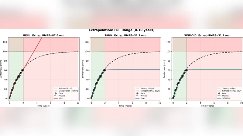
Performance is evaluated on forward prediction accuracy, computational speed, and inverse‑problem efficiency. In the forward wave‑propagation test, PINNs achieve an L2 error roughly 2.5 times larger than a second‑order finite‑difference (FD) scheme while requiring about 90,000 × more wall‑clock time. The slowdown is attributed to the high‑dimensional optimization landscape, repeated automatic differentiation, and the need for penalty terms to enforce boundary conditions. Moreover, PINNs exhibit catastrophic divergence when asked to extrapolate beyond the training domain—a common scenario in field applications where soil properties and loading conditions vary widely.

DeepONet demonstrates that, after an expensive offline training phase, a single inference takes ~1 ms, which is slower than the FD solver (~0.01 ms) but can become advantageous when millions of evaluations are needed, such as in Monte‑Carlo risk assessments or large‑scale parametric sweeps. However, the model’s generalization is tightly bound to the distribution of the training data; predictions for unseen parameter combinations or non‑linear boundary conditions incur a sharp rise in error, indicating that DeepONet is reliable only within its learned envelope.

GNS shows promise for geometry‑agnostic simulation. By representing complex foundation shapes and heterogeneous soil layers as graphs, GNS can produce results about five times faster than the FD baseline for the same spatial resolution. Nevertheless, the method fails to capture path‑dependent soil behavior (e.g., plastic yielding, strain hardening, hysteresis) because the current message‑passing formulation lacks internal state variables that evolve with loading history. Scaling also becomes problematic: as the number of graph nodes exceeds ~10,000, memory consumption and O(N²) computational cost rise sharply, limiting applicability to large field models.

For inverse problems, the authors compare the deep‑learning approaches with a conventional strategy: embedding automatic differentiation (AD) directly into the finite‑element or finite‑difference solver. By treating material parameters (elastic modulus, damping ratio, shear strength, etc.) as differentiable variables and minimizing the misfit between observed and simulated responses, they recover all five target parameters with sub‑percent relative error in under ten seconds. This AD‑enabled inversion outperforms any of the neural‑network‑based surrogates in both speed and accuracy, demonstrating that the most efficient route to parameter identification is to augment proven solvers with modern AD tools rather than to replace them with black‑box neural networks.

Based on these findings, the authors issue several practical recommendations: (1) Do not adopt a deep‑learning surrogate when it is four orders of magnitude slower and less accurate than a traditional solver. (2) Reserve neural‑network models for scenarios where the conventional solver is genuinely computationally prohibitive (e.g., massive Monte‑Carlo studies, real‑time control) and where predictions remain within the training distribution. (3) For inverse analyses, use automatic differentiation through the existing solver; this yields rapid, high‑precision parameter estimates without the overhead of surrogate training. (4) Incorporate site‑based cross‑validation to account for spatial autocorrelation when evaluating model performance on field data. (5) Recognize that extrapolation beyond the training envelope is a critical failure mode for MLP‑based surrogates; rigorous out‑of‑sample testing must precede any deployment.

In summary, the paper provides a balanced, data‑driven assessment of the current state of deep learning in geotechnical engineering. While PINNs, DeepONet, and GNS each bring innovative capabilities—physics‑based loss formulation, operator learning, and geometry‑agnostic graph representations—their practical utility is limited by computational inefficiency, heavy training data demands, poor extrapolation, and an inability to model path‑dependent soil behavior. The authors conclude that, for most engineering practice, traditional numerical methods augmented with automatic differentiation remain the most reliable and efficient tool, and that deep‑learning surrogates should be employed only in narrowly defined, high‑cost computational contexts.