Performance Improvement of Time-Balance Radar Schedulers Through Decision Policies (Extended Version)
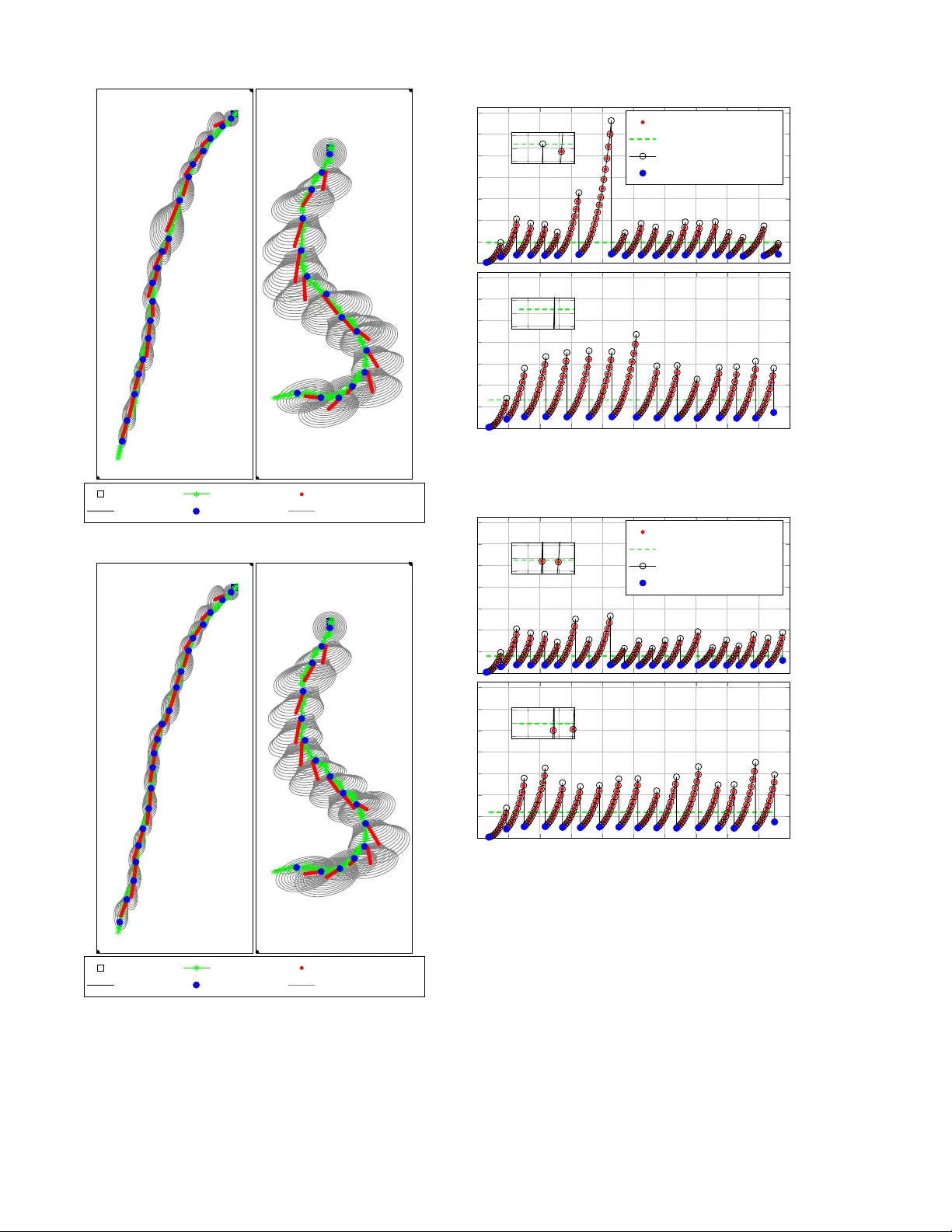
The resource management of a phase array system capable of multiple target tracking and surveillance is critical for the realization of its full potential. Present work aims to improve the performance of an existing method, time-balance scheduling, b…
Authors: "Omer c{C}ay{i}r, c{C}au{g}atay C, an
1 Performance Impro v ement of T ime-Balance Radar Schedulers Through Decision Policies (Extended V ersion) ¨ Omer C ¸ ayır , C ¸ a ˘ gatay Candan Department of Electrical and Electronics Engineering, METU, Ankara, T urke y { ocayir , ccandan } @metu.edu.tr Abstract —The resour ce management of a phase array system capable of multiple target tracking and surveil- lance is critical for the realization of its full potential. Present work aims to impro ve the perf ormance of an existing method, time-balance scheduling, by establishing an analogy with a well-known stochastic contr ol pr oblem, the machine replacement problem. With the suggested policy , the scheduler can adapt to the operational scenario without a significant sacrifice from the practicality of the time-balance schedulers. More specifically , the numerical experiments indicate that the schedulers dir ected with the suggested policy can successfully trade the unnecessary track updates, say of non-maneuvering targets, with the updates of targets with deteriorating tracks, say of rapidly maneuvering targets, yielding an ov erall improvement in the tracking performance. Index T erms —Multi-Function Radar , Radar Resour ce Management, Radar T ask Scheduling, Time-Balance Sched- ulers, Machine Replacement Problem. I . I N T RO D U C T I O N A modern radar system is required to handle a v ariety of tasks, such as surveillance, multi-target tracking, cali- bration, guidance etc. The capabilities of such a system, say a multi-function radar system, come at a significant initial deployment cost mainly due to the installment of possibly thousands of transmit/recei ve modules. T aking the full advantage of the mentioned capabilities requires an effecti ve radar resource management (RRM). T ypi- cally , the multitude of tasks in ex ecution compete for the radar resources, namely time, energy and computation [1], [2], [3]. In this work, we focus on the time allocation problem for such systems. The allocation of time, among other resources, is generally called scheduling in the RRM applications. Scheduling methods can be classified into two classes, adaptiv e and non-adaptiv e methods [1]. Non-adapti ve scheduling methods, namely heuristic schedulers, are based on a rule-based design. The behavior of sched- ulers and prioritization (priority assignment) of tasks are pre-defined by the fixed rules. In contrast, the adaptiv e scheduling methods dynamically determine the task prioritization and scheduling to optimize o verall performance. According to the importance of tasks being scheduled, an ef ficient task prioritization process is re- quired to rank tasks for the performance improvement of both adapti ve and non-adaptiv e schedulers. Kno wledge- based systems using some a-priori information is sug- gested to this aim. Kno wledge-based systems consist of two sub-systems, a kno wledge database containing information related to the system environment and an in- ference engine making final decisions taking into account both a-priori information and e xisting conditions [4]. In [5], a fuzzy logic based approach is suggested to rank targets and surveillance sectors for dynamically changing system en vironments. For tracking tasks, the priorities are assigned according to fi ve dif ferent fuzzy variables such as quality of tracking, hostility , degree of threat. For surveillance tasks, there are four fuzzy variables including the original priority and number of threatening targets. In [6], [7], a neural network based approach is utilized for tar get ranking with respect to range, radial velocity , membership (friend or foe), acceleration and object rank (important or not important). Both neural network and fuzzy logic based approaches provide an adaptiv e priority assignment, in general. Especially , the learning capability of neural network based schedulers enable the operator to update the system behavior after the detection of ne w targets. Ho wev er , the learning pro- cess is far from trivial [2]. The process includes training of several data sets in random order from the same initial starting point [6]. In this work, we aim to achieve the benefits of adap- tiv e scheduling without a major sacrifice from the lo w computational load of non-adaptiv e scheduling methods. More explicitly , the adaptiv e scheduling schemes in the literature are based on the stochastic control and they are, in general, dif ficult to implement due to high computational requirements, [8], [9], [10]. T o reap the benefits of adapti ve scheduling while maintaining a low computational load, we suggest an improv ement over a well-kno wn non-adapti ve scheduling scheme, namely the time-balance scheduler, based on a classical stochas- tic control problem, namely the machine-replacement problem. The suggested improv ement, in effect, yields to an automated task prioritization and shown to hav e good adaptation capabilities to target tracking scenario 2 unfolding to the operator . The time-balance (TB) method is based on the idea of meeting the “deadlines” of each task with the minimum possible delay . The TB method is robust and achieves the desired task occupancies in the long horizon. In Section II, the general features of TB schedulers are further described. A similar adaptation ef fort on the TB method is the adaptiv e task prioritization, as described in [11], with the aim of completing the surveillance task properly even when radar is overloaded with the task of tracking a large number of tar gets and without adjusting the task update times. W ith this method, the task prioritization adapts to a predictable task queue and is independent of radar performance measurements, the track scores. In this work, we aim to dev elop a target selection procedure for the TB method in order to reduce the tracking error , when the radar system is ov erloaded with tracking tasks having identical priorities. The proposed method is based on a well-known stochastic control problem known as the machine replacement problem, as giv en in [12]. Here, our goal is to construct an analogy between the well-known control problem and the tar get tracking problem and enable the utilization of the results for this problem in the performance improv ement of the TB schedulers. The suggested method and its variants are highly practical and can be immediately applied in the existing systems utilizing the con ventional TB schedulers. I I . B A C K G RO U N D : T I M E - B A L A N C E M E T H O D A N D M AC H I N E R E P L AC E M E N T P R O B L E M A. T ime-Balance Method The time-balance metric gi ves the degree of urgency of each task during the radar operation. A revisit time is assigned to each task and the TB metric is continually updated to reflect the approaching visitation deadline of each task, [13], [14]. More specifically , each task is associated with a TB value, t TB . A positiv e t TB value indicates an overdue task. A negati ve t TB value indicates a task whose immediate execution would be ahead of the assigned deadline. A zero t TB value indicates a just- on-time task. At any time, a new task can be inserted to the list by assigning a negati ve t TB value. If a task is scheduled, its t TB is decreased by its task update time (revisit time). Upon execution of any task, the t TB of other tasks which are not scheduled is increased by a fixed amount determined by the designer . Under light load conditions, the TB method is highly ef ficient enabling timely task updates. As the load increases, the TB method suffers a performance loss since this method does not ha ve an y capacity to discriminate tasks as urgent and not-so-urgent. A scheduler algorithm that utilizes the TB method is employed in the Multifunction Electronically Scanned Adaptiv e Radar (MESAR), [13], [15]. This method al- lows to divide tasks into subtasks (looks) that can be interleav ed to manage radar time efficiently and decrease the delays for the highly prioritized tasks by starting from the highest priority lev el at each scheduling instant. In [16], the TB scheduler chooses the task which has higher t TB than other tasks as the next task. The scheduler is designed to schedule mainly the tracking tasks, and the surveillance task is fragmented by the task fragment time. That is, the surveillance task is not periodically started, but one of its fragments is scheduled whenev er all tracking tasks have negati ve t TB value, i.e. when there is some idle time between the tracking tasks. The adaptive time-balance (A TB) scheduler is pro- posed in [11]. Here, the surv eillance task is associated with a t TB value so that it is scheduled with respect to task update time to detect ne w tar gets. The task update times can be adaptively changed as a possible solution for the overload conditions or to increase the revisit improvement factor . The A TB scheduler supports user defined priority le vels for each task, and tasks are scheduled according to these priority lev els and t TB ’ s. In this work, we present a further improvement on the TB method. Our goal is to schedule the tar get tracking tasks according to the track quality . Hence, we would like to ha ve adjust the scheduling parameters of the TB method dynamically according to the unfolding tracking scenario. The tar get selection problem emerges when there are more than one target requesting the track update. The con ventional TB scheduler follows the steps below: 1) Select the targets with the highest priority level, 2) Look for the tar gets which ha ve the highest t TB . T ypically , if there are multiple o verdue tracking tasks at the same priority level, the executed task is selected according to the first-come, first-serve (FCFS) principle, [17, Chapter 6]. This method aims to minimize the ov erall lateness in the task ex ecution. Clearly , this is an efficient mechanism for the maneuvering targets requir - ing a rapid execution depending on the type of maneuver . Our goal is to include the information about track quality in the task selection. T o this aim, we construct an analogy between the well-known machine replacement problem and RRM problem. B. Machine Replacement Problem W e describe the machine replacement problem with a concrete example. Assume a baker having the main asset of an ov en (machine) which can be either in “good” or “bad” state related to its cooking performance. The state of the machine deteriorates due to aging, and the products of the machine can be delicious (conforming) or tasteless (defectiv e) depending on the state v ariable. The true state of the oven is not known, but can be observed by the quality of the products. It is possible to hav e a bad product in spite of the good state of the machine with a non-zero probability and vice versa. In this problem, it is assumed that the cost of a ne w machine (replacement cost), price for the good and bad products are fixed 3 quantities. The main question is to determine the time to replace the machine yielding the profit maximization. This type of optimization problems is categorized as par- tially observable Markov decision processes (POMDPs). Here, the Markov process is related with unknown state of the machine that can be only observed in the presence of noise [18]. W e establish an analogy between the resource man- agement problem and machine replacement problem as follows: For the target selection problem, a target can be in one of two states, namely up-to-date and stale. The up-to-date state denotes that the target track is predictable with a high accuracy by the tracker and may not require an immediate track update. Hence, the up-to- date state can be considered the “good” state. The stale state denotes that the target track is not predictable with a good accurac y and this track may require the urgent attention of the scheduler due to its higher probability of target drop. Hence, it is the “bad” state. As in the POMDP problems, we have noisy information on the target states. As discussed in the latter parts of this paper , we assign a state to each target and utilize the track quality information as the noisy measurement on the state. The proposed analogy is especially v aluable for an o verloaded scheduler; but, e ven for the underloaded case, it can yield some performance improvements. It should be noted that an unnecessary e xecution of a target update in the up- to-date state could decrease the tracking performance of other targets. Hence, the state dependent track update selection can also be beneficial in the improv ement of ov erall track quality . I I I . P RO P O S E D M AC H I N E R E P L AC E M E N T P R O B L E M B A S E D P O L I C Y W e utilize sev eral results, with some corrections, from the work of T . Ben-Zvi, and A. Grosfeld-Nir , [12]. Here, the binomial observation model for the machine replacement problem refers to the classification of the quality of products as conforming units or defective units according to observ ations (measurements) while the production process is in either “good” or “bad” state. The true state of the process is not observable and can only be estimated with some error . Thus, the production process is modeled as a POMDP with some control limits. The POMDPs are kno wn to be usually hard to solve due to prohibitiv ely large size of the state space [19]. In [12], it is proven that the infinite-horizon control limit defined as a function of the probability of obtaining a conforming unit can be calculated by solving a finite set of linear equations. In the target selection problem, there are many tar- gets and each target is, conceptually , associated with a machine. At each instant of decision-making, a target is selected among a set of overdue targets according to the observed track quality depreciations. T o use the machine replacement problem, the cost of the machine renew al, T ABLE I T A R G ET S E L E C TI O N V S . M AC H I N E R EP L AC E M EN T Problem T arget Selection Machine Replacement # of machines > 1 1 States Up-to-date, Good, Stale Bad Observations good track, conforming unit, bad track defectiv e unit Actions update, not-update replace, continue Cost target dependent fixed i.e. the track update, should also be specified. Since there can be only one task scheduled at a time, the cost of ex ecuting a task should include the cost of not-executing the other tasks. The state probabilities are obtained with the interacting multiple model (IMM), as described in [20, Chapter 11]. The mode-probabilities of IMM are associated with the state probabilities of the machine replacement problem. W e assume that there are two motion models, both of which are constant velocity models ha ving dif ferent process noise cov ariance matrices. The cov ariance matrix of two models are gi ven as Q 2 = 100 2 Q 1 , where Q k denotes the cov ariance matrix for the k th model. The case of higher process noise cov ariance matrix refers to the case of a target in the stale state. The other case refers to the up-to-date state. W e can say that the probability of target being in the up-to-date state is taken as the mode-probability of the model- 1 . In addition, the track is considered good; when the trace of IMM mixed cov ariance matrix is within the allowed values. Otherwise, it is considered a bad track. Actions are UPD (update), similar to r eplace the mac hine action comes with a cost K that will be explained later, and NUPD (not-update). In T able I, the analogy between the target selection and machine replacement problem is summarized. In the ne xt section, we provide further details on the analogy gi ven in T able I. A. Pr oblem Model It is supposed that there are N k targets at time k . The target selection problem emerges when there are more than one tar get concurrently requesting the track update among N k targets. Then, the scheduler should decide which one of these tar gets is in need of track update more than others by using the information on the target states. There are N k distinct Marko v chains corresponding to each target, and the state transition probabilities of each target are assumed to be independent. 1) Markov Chain Descriptions: The target- n obeys a 2 -state Markov chain with the follo wing description: • State is x n k ∈ { us, ss } , where us denotes the up-to- date state and ss denotes the stale state, with initial probability P ( x n 0 = i ) = 0 . 5 for i ∈ { us, ss } . • Observation is y n k ∈ { g t, bt } , where g t denotes a good track and bt denotes a bad track. 4 us ss r 1 1 − r (a) Chain for the NUPD action. us ss q 1 − q 1 − q q (b) Chain for the UPD action. Fig. 1. Marko v chains for (a) NUPD (not-update) and (b) UPD (update) actions. • Action is u n k ∈ { NUPD , UPD } , where NUPD de- notes the not-update action and UPD denotes the update action, at time k for n = 1 , 2 , . . . , N k . The state of a target is probabilistically evolving, such that if the target is in up-to-date state at time k , it will remain in that state with probability r or it will change its state to the stale state with probability 1 − r at time k + 1 . Once the target enters the stale state, it is assumed to remain in that state until the UPD action is taken, as shown in Fig. 1(a). Howe ver , the UPD action may fail. A stale target mov es to the up-to-date state with probability q after taking the UPD action, as shown in Fig. 1(b). If the NUPD action is tak en, the transition of target states becomes a time-homogeneous Markov chain with the up-to-date state, a transient state, and the stale state, an absorbing state. The conditional observation probabilities can be ex- pressed as follows: P ( y n k = g t | x n k = us ) = θ 0 , (1) P ( y n k = g t | x n k = ss ) = θ 1 , (2) P ( y n k = bt | x n k = us ) = 1 − θ 0 , (3) P ( y n k = bt | x n k = ss ) = 1 − θ 1 . (4) The expressions given abov e present the probability of having an observation matching the actual state of the target. More specifically , θ 0 denotes the probability of the measurement matching the state of the tar get, i.e. a measurement indicating a good track quality gi v en that the target is in the up-to-date state. 2) Cost Function: Different from the classical ma- chine replacement problem, the cost of updating a spe- cific track (machine renewal) affects the cost of other tracks since there can be only one track that can be updated at an instant, and selecting a specific track for the update action leads to the track quality depreciation of other tracks. W e propose to use the following cost function K n k taking into account the coupling of track quality scores for indi vidual targets: K n k , max n m (0 ,` ) k x ` requesting ,k o N k ` =1 , ` 6 = n m (1 ,n ) k · x n requesting ,k , (5) m (0 ,n ) k m (1 ,n ) k k 0 k − 1 k k + 1 tr P n k 0 tr P n k − 1 tr P n k tr P n k +1 T ime T race of the IMM Mixed Cov ariance IMM Tracking IMM Prediction Fig. 2. Description of the parameters used to find the cost function value. where x n requesting ,k ∈ { 0 , 1 } indicates whether the target- n requests a track update or not. The value of m (1 ,n ) k denotes the estimated improv ement on the IMM mixed cov ariance of the target- n by taking the UPD action u n k = UPD . W e assume that once a target is updated, the diagonal elements of the IMM mix ed cov ariance matrix would be reduced due to the measurement update process. The value of max m (0 ,` ) k N k ` =1 , ` 6 = n denotes the maximum of estimated deterioration on the IMM mixed cov ariance of all targets that are not updated. This set cov ers all targets except the target- n . From (5), it can be noted that the cost of updating target- n is related with the cost of not-updating other targets. The improvement or deterioration metric, m (1 ,n ) k , m (0 ,n ) k , can be taken as the trace of the IMM mixed cov ariance matrix. If the trace decreases at time k + 1 , an improvement on the track quality occurs; otherwise, the track quality deteriorates. Fig. 2 is gi ven to visualize the definitions for m (0 ,n ) k and m (1 ,n ) k are m (0 ,n ) k = tr P n k +1 − tr P n k 0 , (6) m (1 ,n ) k = tr P n k − tr P n k 0 . (7) Here, P n k 0 is the IMM mixed cov ariance matrix of the target- n at time k 0 when the target- n has the latest measured track. W e assume that if track is updated at next time k + 1 , the trace of the IMM mixed cov ariance matrix would be close to the trace of P n k 0 . Hence, m (1 ,n ) k and m (0 ,n ) k depend on P n k 0 . In the next section, we deriv e the expressions required for the solution of target selection problem with the definition presented in this section. B. Derivation of Requir ed Expr essions The probability of being in the up-to-date state is µ n k = P ( x n k = us ) (8) 5 for the target- n at time k . Then, the probability of observing a good track is P g t ( µ n k ) , P ( y n k = g t ) = X i ∈{ us,ss } P ( y n k = g t | x n k = i ) P ( x n k = i ) = ( θ 0 − θ 1 ) µ n k + θ 1 . (9) Similarly , the probability of observing a bad track is P bt ( µ n k ) , P ( y n k = bt ) = X i ∈{ us,ss } P ( y n k = bt | x n k = i ) P ( x n k = i ) = 1 − ( θ 0 − θ 1 ) µ n k − θ 1 . (10) By applying the Bayes’ theorem, the posterior probabil- ities for the up-to-date state are given as P ( x n k = us | y n k = g t ) = P ( y n k = g t | x n k = us ) P ( x n k = us ) P ( y n k = g t ) = θ 0 µ n k P g t ( µ n k ) , (11) P ( x n k = us | y n k = bt ) = P ( y n k = bt | x n k = us ) P ( x n k = us ) P ( y n k = bt ) = (1 − θ 0 ) µ n k P bt ( µ n k ) . (12) W ith the Markov property , it is assumed that x n k +1 is conditionally independent of y n k [21], and hence, the conditional probability of the next state is j giv en that g t is observed and the NUPD action is taken in the current state is i can be written as P ( x n k +1 = j | x n k = i, y n k = g t, u n k = NUPD ) = P ( x n k +1 = j | x n k = i, u n k = NUPD ) = P ij ( u n k ) , (13) where i, j ∈ { us, ss } . By using these expressions and the law of total probability , the conditional probabilities of the next state are obtained. The probability of being in the up-to-date state at next time given that a good track is observed and the NUPD action is taken at current time is expressed as P ( x n k +1 = us | y n k = g t, u n k = NUPD ) = X i ∈{ us,ss } P ( x n k +1 = us, x n k = i | y n k = g t, u n k = NUPD ) = X i ∈{ us,ss } P ( x n k +1 = us | x n k = i, y n k = g t, u n k = NUPD ) P ( x n k = i | y n k = g t, u n k = NUPD ) = X i ∈{ us,ss } ,j = us P ij ( u n k ) P ( x n k = i | y n k = g t ) = r · P ( x n k = us | y n k = g t ) +0 · P ( x n k = ss | y n k = g t ) = r θ 0 µ n k P g t ( µ n k ) , (14) and the probability of being in the up-to-date state at next time given that a bad track is observ ed and the NUPD action is taken at current time is P ( x n k +1 = us | y n k = bt, u n k = NUPD ) = X i ∈{ us,ss } P ( x n k +1 = us, x n k = i | y n k = bt, u n k = NUPD ) = X i ∈{ us,ss } P ( x n k +1 = us | x n k = i, y n k = bt, u n k = NUPD ) P ( x n k = i | y n k = bt, u n k = NUPD ) = X i ∈{ us,ss } ,j = us P ij ( u n k ) P ( x n k = i | y n k = bt ) = r · P ( x n k = us | y n k = bt ) +0 · P ( x n k = ss | y n k = bt ) = r (1 − θ 0 ) µ n k P bt ( µ n k ) . (15) Note that the conditional probabilities gi ven in (14) and (15) can be considered the function of µ n k , since θ 0 and θ 1 are the global constants for the problem. W e use the following notations for the conditional probabilities H g t ( µ n k ) , P ( x n k +1 = us | y n k = g t, u n k = NUPD ) = r θ 0 µ n k ( θ 0 − θ 1 ) µ n k + θ 1 , (16) H bt ( µ n k ) , P ( x n k +1 = us | y n k = bt, u n k = NUPD ) = r (1 − θ 0 ) µ n k 1 − ( θ 0 − θ 1 ) µ n k − θ 1 . (17) According to [19, Lemma 1], both H g t ( µ n k ) and H bt ( µ n k ) are continuous and strictly increasing functions for 0 < µ n k < 1 , while H g t ( µ n k ) is strictly conca ve and H bt ( µ n k ) is strictly conv ex. Moreov er , the in verse func- tions H − 1 g t ( µ n k ) of H g t ( µ n k ) and H − 1 bt ( µ n k ) of H bt ( µ n k ) exist, and they are strictly increasing for 0 < µ n k < r , proofs can be found in [22, Appendix A]. The in verse function H − 1 bt ( µ n k ) is H − 1 bt ( µ n k ) = (1 − θ 1 ) µ n k ( θ 0 − θ 1 ) µ n k + (1 − θ 0 ) r (18) for 0 < µ n k < r . The existence of in verse leads to the use of function composition, i.e. H bt H − 1 bt ( µ n k ) = µ n k . The functions H g t ( µ n k ) and H bt ( µ n k ) depend on the fixed parameters, r , θ 0 and θ 1 as well. The critical point for choosing the fixed parameters is to ensure the criteria, r θ 0 > θ 1 , so that H g t ( µ ∗ ) = µ ∗ > 0 does exist. The value of µ ∗ is computed as µ ∗ = r θ 0 − θ 1 θ 0 − θ 1 . (19) The point, µ ∗ , divides the domain of µ n k into 2 sub- domains, µ ∗ < H g t ( µ n k ) < µ n k for µ n k > µ ∗ and H g t ( µ n k ) > µ n k for 0 < µ n k < µ ∗ . If r θ 0 6 θ 1 , then 0 < H g t ( µ n k ) < µ n k for 0 < µ n k 6 1 , and hence, H g t ( µ ∗ ) = µ ∗ does not exist, as shown in Fig. 3. In Fig. 3(a), parameters satisfy r θ 0 > θ 1 and H g t ( µ ∗ ) = µ ∗ 6 µ ∗ 1 H gt ( µ ∗ ) r 1 µ n k f ( µ n k ) H gt ( µ n k ) H bt ( µ n k ) rµ n k µ n k (a) 1 r 1 µ n k f ( µ n k ) H gt ( µ n k ) H bt ( µ n k ) rµ n k µ n k (b) Fig. 3. The functions H gt ( µ n k ) and H bt ( µ n k ) for (a) r θ 0 > θ 1 , where r = 0 . 8 , θ 0 = 0 . 9 , θ 1 = 0 . 4 , and (b) r θ 0 < θ 1 , where r = 0 . 6 , θ 0 = 0 . 6 , θ 1 = 0 . 4 . exists. If the observation on the state is g t , one knows that the probability of being in the up-to-date state will increase at the next time step, i.e. µ n k +1 > µ n k , for 0 < µ n k < µ ∗ , whereas it will decrease for µ ∗ < µ n k 6 1 , as shown in Fig. 3(a). If µ ∗ does not exist, as shown in Fig. 3(b), then the same probability always decreases, i.e. µ n k +1 < µ n k , irrespective of the observation. Thus, the provided observations can be considered to be informa- tiv e, if µ ∗ exists, i.e. for r θ 0 > θ 1 . The existence of µ ∗ is not critical for the implementation of the scheme, but important for its conceptual understanding. Next, we discuss the value function and associated optimal policy for the infinite-horizon problem where the probability calculations given in this section is required in the computations. 1) Infinite-Horizon V alue Functions: The solution to the stochastic control problem described is studied only for the infinite-horizon case. There is no fixed period which the problem restarts with a giv en set of initial parameters for the target tracking problem. For this problem, each target has a different motion character- istic, and hence, the target-based generalization of initial parameters is not practical. Furthermore, the infinite- horizon case solution has the advantage of requiring less computation. It only requires the computation of a fixed threshold for the asymptotic probability of being in the up-to-date state. Therefore, with a simple threshold policy , whenever the up-to-date state probability is less than the threshold, the optimal action becomes an update action. The optimal action is determined via the optimal value function , V n ( · ) , according to the probability of being in the up-to-date state, µ n k , V n ( µ n k ) = max V n nupd ( µ n k ) , V n upd , (20) where V n nupd ( µ n k ) and V n upd are the infinite-horizon value functions for NUPD and UPD actions, respectively as follows: V n nupd ( µ n k ) = µ n k + α X i ∈{ g t,bt } P i ( µ n k ) V n H i ( µ n k ) = µ n k + α h P g t ( µ n k ) V n H g t ( µ n k ) + P bt ( µ n k ) V n H bt ( µ n k ) i , (21) V n upd = −K n k + V n nupd ( q ) , (22) where α is a discount factor satisfying 0 < α < 1 . The value functions (21) and (22) depend explicitly on each other via V n ( µ n k ) giv en in (20). Furthermore, V n nupd ( µ n k ) , gi ven in (21), is related to the optimal value function, V n ( · ) through the functions H g t ( µ n k ) and H bt ( µ n k ) , while V n ( · ) , given in (20), is already related to V n nupd ( · ) . It is not possible to express V n nupd ( µ n k ) without any assumptions on H g t ( µ n k ) and H bt ( µ n k ) . Choosing θ 1 = 0 , as stated in [12], is a practical choice which assumes that the probability of observing a good track gi ven that corresponding target is in the stale state is 0 and it also av oids always-decreasing probability of the up-to-date state by ensuring rθ 0 > θ 1 , i.e. the existence of µ ∗ . Then, it is only possible that a good track is observed from a target in the up-to-date state. W ith this assumption, (21) can be simplified as V n nupd ( µ n k ) = µ n k + α θ 0 µ n k V n ( r ) +(1 − θ 0 µ n k ) V n H bt ( µ n k ) . (23) Another simplification on the parameter q , the proba- bility of transition to the up-to-date state upon the update action, as shown in Fig. 1(b), is required. T o make the model more realistic, perhaps pessimistic, we take q = r , ( r 6 = 1 ), meaning that update action may f ail (due to radar sensing en vironment). Then, (22) becomes V n upd = −K n k + V n nupd ( r ) . (24) In order to e v aluate the value of V n nupd ( r ) from (23), we need V n ( r ) = max V n nupd ( r ) , V n upd = max K n k + V n upd , V n upd . (25) Since K n k giv en in (5) cannot be negati v e valued, the equation (25) becomes V n ( r ) = K n k + V n upd . (26) 7 K n k µ n th B 1 B 2 r α 3 V n upd α 2 V n upd αV n upd V n upd V n nupd ( r ) V n nupd ( µ n k ) H 3 bt ( r ) H 2 bt ( r ) H bt ( r ) Fig. 4. The value function of NUPD action for M = 3 . By using (26), the simplified value function of NUPD action, (23) becomes V n nupd ( µ n k ) = µ n k + α θ 0 µ n k K n k + V n upd +(1 − θ 0 µ n k ) V n H bt ( µ n k ) . (27) 2) The Thr eshold V alue for Decision-Making: The threshold value for the target- n , which is denoted as µ n th , is the solution of V n nupd ( µ n k ) = V n upd , where LHS and RHS are gi ven in (27) and (24) respectiv ely . Then, the decision-making process is gi ven as u n k = ( NUPD , µ n k > µ n th UPD , otherwise (28) such that the action is no-update on the track if the threshold is exceeded. It is not straightforward to obtain (24) and (27) o wing to the presence of V n nupd ( r ) in (24). Fig. 4 is gi ven to visualize the value function of NUPD action obtained from the basic parameters, α , θ 0 , r , K n k . The function V n nupd ( µ n k ) is the pointwise maximum of linear functions cutting µ n k = 0 axis at α 3 V n upd , α 2 V n upd and αV n upd for 0 6 µ n k 6 1 . Thus, it is a piecewise linear con ve x function, see [12, Theorem 2]. The intersection points of these linear functions are the breakpoints of V n nupd ( µ n k ) such that B 1 = H − 1 bt ( µ n th ) and B 2 = H − 1 bt ( B 1 ) . The number of linear functions, namely linear segments of V n nupd ( µ n k ) , M , is determined with µ n th satisfying r > H bt ( r ) > H 2 bt ( r ) > · · · > H M − 2 bt ( r ) > H M − 1 bt ( r ) > µ n th > H M bt ( r ) , see [12, Corollary 1]. T o obtain M , the constraint H M bt ( r ) < µ n th is utilized, where H M bt ( r ) is found by e valuating (17) recursi vely . For each M value starting from M = 1 , µ n th is computed and compared with H M bt ( r ) until the constraint holds. The expression of µ n th depending on M and the basic parameters will be provided later . The relation between µ n th and V n upd can be found from (27) at µ n k = µ n th by replacing V n nupd ( µ n th ) and V n H bt ( µ n th ) with V n upd , where the latter is the result of H bt ( µ n th ) < µ n th , as shown in Fig. 3(a). Then, µ n th can be computed as µ n th = 1 − α 1 + αθ 0 K n k V n upd , (29) if V n upd is known, see [12, Proposition 4]. Thus, the value of V n upd is the most critical point of the calculations. The expression of V n upd depending on M and the basic parameters is found by solving M + 1 distinct equations, V n ( r ) , V n H bt ( r ) , . . . , V n H M − 1 bt ( r ) from (23) ow- ing to V n ( µ n k ) = V n nupd ( µ n k ) for µ n k > µ n th , and V n H M bt ( r ) = V n upd . Then, V n upd can be computed by V n upd , A M ( r )(1 + αθ 0 K n k ) − K n k 1 − αθ 0 A M ( r ) − B M ( r ) , (30) where A M ( r ) is defined as A M ( r ) , r , M = 1 r + M − 1 X i =1 α i H i bt ( r ) i − 1 Q j =0 1 − θ 0 H j bt ( r ) , M > 2 (31) and B M ( r ) is defined as B M ( r ) , M − 1 Y i =0 α 1 − θ 0 H i bt ( r ) , (32) for M > 1 by supposing that V n nupd ( µ n k ) consists of M segments, see [12, Theorem 3 and 4]. Deriv ations of A M ( r ) and B M ( r ) can be found in [22, Chapter 4]. A careful examination of (30) rev eals that V n upd can be negati ve v alued depending on the K n k value. If K n k is high enough, then V n upd is negati v e valued, and hence, µ n th also becomes also negati v e according to (29). Therefore, the NUPD action immediately becomes the optimal action for the ne gativ e threshold v alues since µ n k is alw ays positiv e. This observation simplifies the computations for the decision-making process, since it is possibly to infer whether µ n th is negati ve or not, from K n k . When K n k > r / (1 − αr ) , a degenerate policy emerges and the optimal action is always NUPD [23, Proposition 2], see the proof of Proposition 3 [22, Chapter 4]. Then, the threshold v alue is determined by µ n th = 0 , K n k > r 1 − αr 1 − α 1 + αθ 0 K n k V n upd , otherwise. (33) The computation of threshold µ n th is explicitly de- scribed in T able II. Here, line 2 checks whether the parameters cause a degenerate policy or not. Lines 5 to 18 start with M = 1 and increase M until H M bt ( r ) < µ n th is satisfied, meanwhile, µ n th is computed by ev aluating (17), (31), (32), (30) and (33) respectively . W e present the outputs of the algorithm in T able II for some special cases in T able III. This table can also 8 T ABLE II A L GO R I T HM F O R C O MP U T I NG T H E T H RE S H O LD V A LU E 1: function T H R ES H O L D α, θ 0 , r , K n k 2: if K n k > r / (1 − αr ) then 3: µ n th = 0 4: else 5: M = 1 6: compute H M bt ( r ) from (17) 7: compute A M ( r ) from (31) 8: compute B M ( r ) from (32) 9: compute V n upd from (30) 10: compute µ n th from (33) 11: while H M bt ( r ) > µ n th do 12: M + + 13: compute H M bt ( r ) from (17) 14: compute A M ( r ) from (31) 15: compute B M ( r ) from (32) 16: compute V n upd from (30) 17: compute µ n th from (33) 18: end while 19: end if 20: retur n µ n th 21: end T ABLE III C O MPA R IS O N O F T H E T H R E SH O L D V AL U E A N D N U M B ER O F S E GM E N T S F OR D I FF ER E N T K n k V AL U E S W I TH α = 0 . 99 r = 0 . 90 r = 0 . 95 K n k θ 0 0 . 75 0 . 80 0 . 90 0 . 75 0 . 80 0 . 90 0 . 1 µ n th 0 . 8069 0 . 8073 0 . 8082 0 . 8569 0 . 8573 0 . 8582 M 1 1 1 1 1 1 1 . 0 µ n th 0 . 3984 0 . 3933 0 . 3799 0 . 4667 0 . 4611 0 . 4464 M 2 2 2 2 2 2 2 . 5 µ n th 0 . 1809 0 . 1755 0 . 1730 0 . 2503 0 . 2429 0 . 2315 M 3 3 2 3 3 2 be used for debugging purposes. Here, we assume that α = 0 . 99 and other basic parameters, θ 0 , r and K n k are changed to obtain distinct infinite-horizon value func- tions. The algorithm outputs, namely the threshold values and the numbers of segments, are giv en in T able III. Some comments on the data of T able III can be giv en as follows: • The higher r makes µ n th higher since A M ( r ) in- creases with r , and V n nupd also increases. This statement can be deduced from (30). • The higher K n k makes µ n th smaller . That is K n k < r / (1 − αr ) ∧K n k → r / (1 − αr ) = ⇒ µ n th → 0 . • M depends on both θ 0 and K n k , as illustrated more clearly for K n k = 2 . 5 in T able III. Up to now , we hav e discussed how to decide whether a single tar get requires an update action or not based on its estimated track accuracy and calculated threshold giv en by the suggested algorithm. For the multiple target tracking scenarios, there can be a situation that se veral targets requiring an update at the same time, i.e. the up- to-date state probability falls below the corresponding threshold lev el. For such cases, we need to dev elop a policy for the selection of the most suitable tar get. C. Pr oblem Solution: T ar get Selection P olicies W e present three policies for the selection of the track to be updated. The first policy is based on the machine replacement problem and uses the threshold policy for the selection of track. The other policies use IMM outputs, but not the threshold value; hence, they are simpler to implement. 1) Decision P olicy (DecP): This policy selects the track to be updated among the tracks satisfying the condition µ n k < µ n th for n = { 1 , 2 , . . . , N k } . It should be remembered that this condition is analogous to the decision of machine replacement. The decision policy (DecP) selects the target- i accord- ing to i = argmin n ∈{ 1 , 2 ,...,N k } { µ n k − µ n th } . (34) sub ject to x n requesting ,k = 1 µ n k < µ n th Ideally , the condition µ n k < µ n th should be satisfied only if the track is sufficiently degraded. If none of the tracks is not sufficiently degraded, there is no track update. Hence, under the ideal conditions, the radar resources are not wasted by updating the tracks solely by the lateness value. It should be remembered that this method has multiple criterion to be satisfied to grant a track update. First, by the requirement of the TB method, t TB value should be non-negati ve; hence, the lateness parameter should be either zero or a positiv e number . Second, the track should be sufficiently degraded, which is a condition checked by µ n k < µ n th . Third, among all tracks satisfying first two conditions, the track with the highest gap to threshold is selected. 2) T rac king Error Minimization P olicy (MinTE): This is a greedy policy implementing the update of the track based on the IMM mixed cov ariance matrices of the targets. The aim is to select the target among the set of targets with non-negati ve t TB value and the worst case tracking error . T o select the tar get- i , this method tak es into account the mixed cov ariance matrix, but not the mode-probabilities of IMM: i = argmax n ∈{ 1 , 2 ,...,N k } n tr P n k o . (35) sub ject to x n requesting ,k = 1 It should be noted that the target with the highest trace of IMM mixed covariance matrix may not necessarily correspond to a rapidly maneuvering target. This policy does not ex ert any ef fort in detecting the maneuv ering action of the tar get. 9 3) Pursuing the Most Maneuvering T arget P olicy (PurMM): It should be remembered that the probability of up-to-date state is giv en as µ n k . Then, the updated target can be chosen according to the product of the trace of IMM mixed cov ariance matrix and the stale state probability , 1 − µ n k : i = argmax n ∈{ 1 , 2 ,...,N k } n (1 − µ n k ) tr P n k o . (36) sub ject to x n requesting ,k = 1 This method aims to giv e higher priority to the tar gets with having a high probability of maneuvering, namely probability of the mode with high process noise. Hence, this method is called as the method of pursuing the most maneuvering target (PurMM). I V . N U M E R I C A L C O M PA R I S O N S The assumed instrumented range for the simulator is 200 km. W ithin this detection range, the assigned priority changes from 1 to 5 according to the detected tar get range with a range step of 40 km. For example, the target at the range of 60 km is assigned to the priority lev el 4 , which is the second highest priority lev el. The measurement noise is N (0 , σ 2 r ) and N (0 , σ 2 a ) for range and azimuth, respectiv ely , where σ r = 80 m and σ a = 3 mrad. Further details on radar simulator can be found in [22]. Due to the nature of conv entional TB scheduler , the target selection policies are applied on the targets with the same priority . Hence, the tracking error of targets at only similar ranges are compared by these policies. A. Case 1: Single T arg et T rac king Case T o illustrate the improvement brought by the DecP , we compare the performance of TB method utilizing the DecP with the con ventional TB method. The conv en- tional TB method does not utilize the track information provided by IMM. Hence, its performance is expected to be inferior to the one utilizing the DecP . Our goal is to contrast the difference between the two. The Fig. 5(a) sho ws the performance of con v entional method on non-maneuvering (left panel of Fig. 5(a)) and maneuvering (right panel) tar gets. The tracking perfor- mance of the TB method with DecP is given in Fig. 5(b). In this figure, the confidence ellipses are drawn to illustrate the tracking performance. A visual comparison of top and bottom panels of Fig. 5 immediately re veals that the DecP yields a better performance by refraining from, or postponing, unnecessary track updates. More specifically , for the non-maneuvering target, the average tracking error , namely the a verage of the trace of IMM mixed covariance matrices, decreases from 1 . 93 × 10 5 m 2 , given in the top part of Fig. 6(a), to 1 . 59 × 10 5 m 2 , gi ven in the top part of Fig. 6(b). For the maneuvering target, the av erage tracking error decreases from 2 . 63 × 10 5 m 2 to 2 . 39 × 10 5 m 2 . Furthermore, the maximum value of the tracking error is also smaller with the DecP , which is a criterion that can be especially important for rapidly maneuv ering targets. Howe v er , it is important to remind that the DecP does not guarantee a better operation at every run, but can present significant improvements in the scenarios where the beginning of target maneuv ering can be effecti vely sensed with the IMM mode-probabilities. B. Case 2: Multiple T arg et T rac king Case The proposed methods are e v aluated for the scenario of multiple targets in addition to the surveillance tasks. The target tracks are randomly generated for each scenario of 200 seconds. Each target has randomly chosen transition probability matrix out of fi ve matrices, while the IMM tracker makes use of fixed transition probabilities for all tracks. There are 100 distinct scenarios for each comparison case. The comparisons are made on the av erage of the scheduler performance that is measured with the following criteria: • The number of pr obable dr ops is the number of updates that are too late for target tracking. The probable drop occurs when the update interval ex- ceeds the sum of task update time and allowable lateness. • Cost is the sum of weighted lateness values squares after each scheduling epochs. The priority v alues are assigned as the weights. • A ver age of err ors is the av erage of the trace of IMM mixed cov ariance matrices of all tar gets. • Occupancy is the ratio of utilized radar time to the total av ailable time interv al. In T able IV and V, the suggested methods are com- pared for the scenarios of 15 and 25 in-track-targets, respectiv ely . Our main goal is to compare the perfor- mance statistics resulting from the application of the con ventional TB method and TB method augmented with the suggested policies. In order to illustrate the effect of the loading condition more explicitly , we assume that the radar system can uti- lize multiple-frequenc y bands concurrently . An increase in the number of frequency bands reduces the load seen from the resource management side [22]. The number of frequency bands is selected as 2 in T able IV(a) and V(a), and the number of bands is selected as 7 in T able IV(b) and V(b). When the proposed methods, (DecP , MinTE and PurMM) are compared with the con ventional TB method, it can be seen that the DecP is the method which has the smallest number of probable drops and the smallest av erage of errors for all cases. Y et, the alternativ es to the DecP (MinTE and PurMM) are almost equally good for this case. T ables also illustrate the performance comparison of the methods in a competitive sense. From the bottom part of the tables, it can be noted the con ventional method has most frequently provided the poorest tracking error per- formance for the duration of complete scenarios, while the DecP has the smallest number of bad performances. 10 Initial Track Measurements IMM Tracking T rue Tracks Detections Confidence Ellipses S 1 S 2 S 3 ( − 145 . 8 km , − 7 km ) ( − 128 . 2 km , 37 km ) S 1 S 2 S 3 ( − 46 km , 141 . 5 km ) ( − 36 km , 166 . 5 km ) (a) The conventional TB method. Initial Track Measurements IMM Tracking T rue Tracks Detections Confidence Ellipses S 1 S 2 S 3 ( − 145 . 8 km , − 7 km ) ( − 128 . 2 km , 37 km ) S 1 S 2 S 3 ( − 46 km , 141 . 5 km ) ( − 36 km , 166 . 5 km ) (b) The TB method with DecP . Fig. 5. T racking of non-maneuvering (left) and maneuvering (right) targets by using (a) conv entional TB method and (b) TB method with DecP . In T able VI, the distributions of standings given in T able IV and V are combined for a clearer comparison. T able VI indicates that the DecP is the most frequently 0 2 4 6 8 10 12 14 10 20 1 . 8 1 . 9 2 × 10 5 T race of the IMM Mixed Covariance ( × 10 5 m 2 ) IMM Tracking A vg. of IMM Tracking IMM Prediction Detections 0 20 40 60 80 100 120 140 160 180 200 0 2 4 6 8 10 12 14 10 20 2 . 5 2 . 6 2 . 7 × 10 5 T ime (s) (a) The conventional TB method. 0 2 4 6 8 10 12 14 10 20 1 . 5 1 . 6 1 . 7 × 10 5 T race of the IMM Mixed Covariance ( × 10 5 m 2 ) IMM Tracking A vg. of IMM Tracking IMM Prediction Detections 0 20 40 60 80 100 120 140 160 180 200 0 2 4 6 8 10 12 14 10 20 2 . 3 2 . 4 2 . 5 × 10 5 T ime (s) (b) The TB method with DecP . Fig. 6. Trace of IMM mixed covariance matrices for non-maneuvering (top) and maneuvering (bottom) targets by using (a) conv entional TB and (b) TB method with DecP . successful policy among the four . It can be said that the DecP successfully traded the unnecessary track updates of targets having accurately predictable tracks, e.g. non- maneuvering targets, with the track quality depreciating targets, e.g. maneuvering targets. This conclusion can be further justified by examining the a verage of errors criteria in the tables where the DecP is the best policy in all cases. Hence, as in the single target case, the DecP , in essence, manages to “detect” the beginning of 11 T ABLE IV C O MPA R IS O N O F T H E D E C I SI O N P O L I CI E S F O R 15 T A R GE T S (a) The number of frequency bands is 2 . A verage of statistics after 100 simulations Con v . DecP MinTE PurMM # of tracking tasks 288 . 91 292 . 11 289 . 73 289 . 20 # of surveillances 17 . 52 17 . 43 17 . 37 17 . 52 # of prob. drops 23 . 76 23 . 04 23 . 12 23 . 08 Occupancy ( % ) 48 . 43 48 . 69 48 . 37 48 . 47 Cost (s 2 ) 9 . 13 × 10 4 1 . 01 × 10 5 9 . 49 × 10 4 1 . 11 × 10 5 A vg. of errors (m 2 ) 4 . 70 × 10 5 3 . 69 × 10 5 3 . 97 × 10 5 4 . 64 × 10 5 Distributions of standings in avg. of errors Best 20 38 19 23 Runner-up 24 24 33 19 Honorable Mention 25 21 30 24 Last 31 17 18 34 (b) The number of frequency bands is 7 . A verage of statistics after 100 simulations Con v . DecP MinTE PurMM # of tracking tasks 502 . 54 504 . 67 504 . 22 503 . 18 # of surveillances 19 . 13 19 . 10 18 . 98 19 . 09 # of prob. drops 8 . 38 8 . 22 8 . 39 8 . 30 Occupancy ( % ) 74 . 17 74 . 32 74 . 18 74 . 15 Cost (s 2 ) 9 . 49 × 10 2 8 . 13 × 10 2 7 . 28 × 10 2 9 . 58 × 10 2 A vg. of errors (m 2 ) 8 . 95 × 10 4 8 . 77 × 10 4 8 . 82 × 10 4 8 . 89 × 10 4 Distributions of standings in avg. of errors Best 20 26 32 22 Runner-up 24 30 17 29 Honorable Mention 16 35 26 23 Last 40 9 25 26 a maneuver successfully and does not grant unnecessary updates to a track in spite of its potentially large lateness value. Interested readers may examine [22] for more comparisons. C. Comparisons with T ask Prioritization Methods W e compare the con v entional TB and DecP with two other task prioritization methods based on neural netw ork [6], [7] and fuzzy logic [5]. The detailed descriptions on these methods such as the choice of training set for the neural network based scheme and the membership functions for the fuzzy logic based scheme can be found in Appendix. Similar to the decision policies, these methods incorporate the tracking error into decision- making. In addition, they use some other inputs such as the radial v elocity and the allo wable lateness for the task prioritization. Unlike the decision policies, which are applied only when the con ventional TB requires selecting one of targets having the same priority lev el, the task prioritization methods are continually applied. In T able VII and VIII, the DecP is compared with the task prioritization methods for 15 and 25 targets, respectiv ely . From the viewpoint of minimum average T ABLE V C O MPA R IS O N O F T H E D E C I SI O N P O L I CI E S F O R 25 T A R GE T S (a) The number of frequency bands is 2 . A verage of statistics after 100 simulations Con v . DecP MinTE PurMM # of tracking tasks 294 . 93 296 . 39 296 . 66 298 . 07 # of surveillances 24 . 55 24 . 55 24 . 40 24 . 63 # of prob. drops 38 . 40 37 . 37 37 . 98 37 . 94 Occupancy ( % ) 55 . 70 55 . 84 55 . 72 56 . 11 Cost (s 2 ) 5 . 21 × 10 5 5 . 22 × 10 5 4 . 79 × 10 5 5 . 28 × 10 5 A vg. of errors (m 2 ) 8 . 73 × 10 5 7 . 44 × 10 5 8 . 60 × 10 5 8 . 14 × 10 5 Distributions of standings in avg. of errors Best 20 28 18 34 Runner-up 26 31 21 22 Honorable Mention 25 24 32 19 Last 29 17 29 25 (b) The number of frequency bands is 7 . A verage of statistics after 100 simulations Con v . DecP MinTE PurMM # of tracking tasks 538 . 33 538 . 74 537 . 18 537 . 53 # of surveillances 25 . 86 25 . 94 26 . 02 26 . 10 # of prob. drops 39 . 48 39 . 33 40 . 48 40 . 10 Occupancy ( % ) 83 . 76 83 . 88 83 . 79 83 . 92 Cost (s 2 ) 1 . 68 × 10 5 1 . 89 × 10 5 1 . 80 × 10 5 1 . 89 × 10 5 A vg. of errors (m 2 ) 3 . 35 × 10 5 3 . 28 × 10 5 3 . 49 × 10 5 3 . 58 × 10 5 Distributions of standings in avg. of errors Best 22 35 21 22 Runner-up 35 25 21 19 Honorable Mention 21 28 16 35 Last 22 12 42 24 T ABLE VI O V E RA L L D I S T RI B U TI O N S O F S TAN D I N GS I N A V E RA GE O F E R RO R S A F TE R 400 S I MU L A T I O NS Con v . DecP MinTE PurMM Best 82 127 90 101 Runner-up 109 110 92 89 Honorable Mention 87 108 104 101 Last 122 55 114 109 tracking error , the DecP policy remains as the best choice. On the other hand, the task prioritization methods provides the minimum number of probable drops due to the inclusion of the allo wable lateness parameter in the scheduler design. V . C O N C L U S I O N S In this work, we adapt the solution methods for the well-known machine replacement problem to the RRM problem. W e propose practical performance improvement policies for the TB method. The con ventional TB method does not hav e the capacity to adapt to the unfolding target tracking scenario. T o provide some adaptation 12 T ABLE VII C O MPA R IS O N W I T H T AS K P R I O RI T I Z A TI O N M E T H OD S F O R 15 T A R G ET S (a) The number of frequency bands is 2 . A verage of statistics after 100 simulations Con v . DecP Neural N. Fuzzy L. # of tracking tasks 288 . 91 292 . 11 287 . 21 283 . 26 # of surveillances 17 . 52 17 . 43 16 . 70 16 . 61 # of prob. drops 23 . 76 23 . 04 21 . 75 21 . 34 Occupancy ( % ) 48 . 43 48 . 69 47 . 46 47 . 16 Cost (s 2 ) 9 . 13 × 10 4 1 . 01 × 10 5 1 . 29 × 10 5 1 . 56 × 10 5 A vg. of errors (m 2 ) 4 . 70 × 10 5 3 . 69 × 10 5 5 . 13 × 10 5 6 . 94 × 10 5 Distributions of standings in avg. of errors Best 21 49 24 6 Runner-up 37 25 22 16 Honorable Mention 22 19 35 24 Last 20 7 19 54 (b) The number of frequency bands is 7 . A verage of statistics after 100 simulations Con v . DecP Neural N. Fuzzy L. # of tracking tasks 502 . 54 504 . 67 509 . 66 509 . 08 # of surveillances 19 . 13 19 . 10 18 . 56 18 . 48 # of prob. drops 8 . 38 8 . 22 7 . 45 7 . 58 Occupancy ( % ) 74 . 17 74 . 32 74 . 38 74 . 22 Cost (s 2 ) 9 . 49 × 10 2 8 . 13 × 10 2 7 . 90 × 10 2 4 . 95 × 10 3 A vg. of errors (m 2 ) 8 . 95 × 10 4 8 . 77 × 10 4 8 . 88 × 10 4 9 . 49 × 10 4 Distributions of standings in avg. of errors Best 15 36 32 17 Runner-up 31 28 23 18 Honorable Mention 32 27 21 20 Last 22 9 24 45 capability , we present a decision policy , DecP , and two other alternativ es. The results show that DecP based TB method yields better tracking performance, by trading the unnecessary updates of targets having accurately predictable tracks with the tar gets suffering from track quality de gradations, say maneuvering targets. This is achiev ed, in ef fect, with the early detection of the track quality degradations via the utilization of information provided by IMM filter in the decision-making. In the numerical comparisons, it has been noted that the suggested DecP based TB method is the method with the fewest worst case tracking performance. Furthermore, the suggested policy does not only improve the average tracking performance, but can also reduce the tar get drops. The suggested polic y is also compared with the knowledge-based task prioritization methods based on neural networks and fuzzy logic. The neural network based scheme shows a competitiv e performance due to the efficient training process, while the fuzzy logic shows a rather poor performance and requires more computational time due to large number of rules. Thus, T ABLE VIII C O MPA R IS O N W I T H T AS K P R I O RI T I Z A TI O N M E T H OD S F O R 25 T A R G ET S (a) The number of frequency bands is 2 . A verage of statistics after 100 simulations Con v . DecP Neural N. Fuzzy L. # of tracking tasks 294 . 93 296 . 39 290 . 72 276 . 92 # of surveillances 24 . 55 24 . 55 23 . 84 23 . 62 # of prob. drops 38 . 40 37 . 37 35 . 03 35 . 99 Occupancy ( % ) 55 . 70 55 . 84 54 . 58 53 . 16 Cost (s 2 ) 5 . 21 × 10 5 5 . 22 × 10 5 5 . 76 × 10 5 7 . 10 × 10 5 A vg. of errors (m 2 ) 8 . 73 × 10 5 7 . 44 × 10 5 9 . 23 × 10 5 1 . 36 × 10 6 Distributions of standings in avg. of errors Best 24 38 30 8 Runner-up 39 36 16 9 Honorable Mention 25 14 35 26 Last 12 12 19 57 (b) The number of frequency bands is 7 . A verage of statistics after 100 simulations Con v . DecP Neural N. Fuzzy L. # of tracking tasks 538 . 33 538 . 74 538 . 31 519 . 42 # of surveillances 25 . 86 25 . 94 25 . 27 25 . 31 # of prob. drops 39 . 48 39 . 33 35 . 29 36 . 96 Occupancy ( % ) 83 . 76 83 . 88 83 . 24 81 . 53 Cost (s 2 ) 1 . 68 × 10 5 1 . 89 × 10 5 2 . 45 × 10 5 3 . 70 × 10 5 A vg. of errors (m 2 ) 3 . 35 × 10 5 3 . 28 × 10 5 4 . 55 × 10 5 6 . 15 × 10 5 Distributions of standings in avg. of errors Best 35 48 16 1 Runner-up 46 36 15 3 Honorable Mention 13 10 53 24 Last 6 6 16 72 the capabilities of knowledge-based methods are limited by training process or inference rules. The suggested decision policy is rather simple and does present a good track quality improv ement according to se veral performance metrics. A C K N O W L E D G M E N T Authors would like to thank Prof. Umut Or guner for his kind support, suggestions and insightful comments. A P P E N D I X D E S C R I P T I O N S O F T H E T A S K P R I O R I T I Z A T I O N M E T H O D S E V A L UA T E D F O R C O M PA R I S O N S T ask prioritization methods based on neural network [6], [7] and fuzzy logic [5] could not be implemented directly as described in references, due to distinctions between problem models. W e define common input v ari- ables to adapt these methods to our radar system and to fairly compare them. Input v ariables are as follo ws: • P osition v ariable denotes the normalized position of a tar get relati ve to the innermost point of a priority ring within the same azimuth angle, e.g. 13 T ABLE IX T R AI N I N G S ET F O R N E U RA L N E TW O R K # Position Radial V elocity (m/s) T rack In validity Allow able Lateness (s) Original Priority T racking T ask Priority 1 0 . 9939 22 . 69 0 . 0093 0 . 60 2 0 . 0897 2 0 . 7425 71 . 45 0 . 1832 1 . 60 4 0 . 7205 3 0 . 5375 14 . 11 0 . 0994 2 . 20 4 0 . 6457 4 0 . 6775 50 . 11 0 . 2483 2 . 60 4 0 . 6538 5 0 . 2919 62 . 64 0 . 0091 2 . 40 3 0 . 3327 6 0 . 5132 263 . 77 0 . 1026 0 . 60 1 0 . 0862 7 0 . 2254 59 . 40 0 . 1009 3 . 00 4 0 . 6791 8 0 . 7661 203 . 99 0 . 1018 1 . 40 4 0 . 7838 9 0 . 7286 10 . 87 0 . 9692 3 . 00 2 0 . 1834 10 0 . 0413 68 . 90 0 . 4899 2 . 60 1 0 . 0653 11 0 . 5298 184 . 62 0 . 9997 1 . 20 2 0 . 5207 12 0 . 4498 103 . 32 0 . 2454 2 . 80 2 0 . 1186 13 0 . 5654 63 . 38 0 . 0556 1 . 20 5 0 . 9282 14 0 . 5030 108 . 20 0 . 1226 1 . 40 2 0 . 1599 15 0 . 0576 54 . 26 0 . 0093 2 . 20 3 0 . 4062 16 0 . 5449 220 . 20 0 . 0095 1 . 40 1 0 . 0463 17 0 . 4213 15 . 02 0 . 0587 2 . 20 4 0 . 6600 18 0 . 4893 43 . 44 0 . 0919 2 . 20 5 0 . 9018 19 0 . 5617 117 . 48 0 . 0895 1 . 20 4 0 . 7867 20 0 . 5354 10 . 40 0 . 0887 3 . 20 1 0 . 0133 21 0 . 1073 173 . 59 0 . 0514 2 . 00 5 0 . 9554 22 0 . 4214 14 . 72 0 . 4778 2 . 80 1 0 . 0337 23 0 . 4880 10 . 45 0 . 1452 2 . 00 2 0 . 1028 24 0 . 0354 212 . 71 0 . 5316 0 . 60 1 0 . 2161 25 0 . 1571 48 . 07 0 . 0093 2 . 00 2 0 . 1291 26 0 . 0586 197 . 90 0 . 8060 1 . 40 1 0 . 2234 27 0 . 1100 61 . 46 0 . 0090 2 . 40 3 0 . 3776 28 0 . 9812 51 . 07 0 . 1311 2 . 80 3 0 . 1887 29 0 . 4913 138 . 69 1 . 0000 2 . 60 1 0 . 1095 30 0 . 4234 63 . 91 0 . 1501 2 . 00 4 0 . 7409 31 0 . 8144 142 . 09 0 . 1902 1 . 60 3 0 . 4053 32 0 . 1320 11 . 84 0 . 2947 3 . 20 2 0 . 1159 33 0 . 6585 154 . 45 0 . 2427 1 . 60 1 0 . 0449 34 0 . 0717 54 . 23 0 . 1179 3 . 00 3 0 . 3649 35 0 . 8461 137 . 78 0 . 9992 0 . 60 3 0 . 7902 # Position Radial V elocity (m/s) T rack In validity Allow able Lateness (s) Original Priority T racking T ask Priority 36 0 . 6705 159 . 16 0 . 0369 0 . 80 5 0 . 9471 37 0 . 9792 150 . 03 0 . 0669 1 . 60 5 0 . 9026 38 0 . 8751 61 . 95 0 . 0686 2 . 20 5 0 . 8597 39 0 . 6780 63 . 46 0 . 0499 2 . 60 4 0 . 5866 40 0 . 6825 51 . 20 0 . 0095 1 . 80 1 0 . 0203 41 0 . 6074 108 . 30 0 . 2895 2 . 00 5 0 . 9372 42 0 . 8189 33 . 63 0 . 0427 2 . 40 5 0 . 8401 43 0 . 9859 83 . 21 0 . 6677 3 . 00 3 0 . 3632 44 0 . 8068 10 . 13 0 . 2872 2 . 80 3 0 . 2428 45 0 . 3788 41 . 13 0 . 7067 2 . 20 2 0 . 2482 46 0 . 8867 62 . 63 0 . 0093 2 . 40 2 0 . 0555 47 0 . 9127 30 . 27 0 . 0930 2 . 60 4 0 . 5146 48 0 . 6896 82 . 32 0 . 0587 2 . 60 5 0 . 8694 49 0 . 7627 61 . 15 0 . 5034 2 . 80 3 0 . 3608 50 0 . 2818 66 . 24 0 . 0094 2 . 60 1 0 . 0235 51 0 . 7048 60 . 13 0 . 3315 3 . 00 3 0 . 2932 52 0 . 5438 34 . 47 0 . 1127 3 . 20 4 0 . 5637 53 0 . 0727 74 . 72 0 . 0879 1 . 40 2 0 . 2061 54 0 . 9995 35 . 23 0 . 1029 3 . 20 3 0 . 1488 55 0 . 1679 102 . 10 0 . 0669 1 . 40 5 0 . 9549 56 0 . 3996 229 . 30 1 . 0000 0 . 60 3 0 . 8915 57 0 . 4460 190 . 43 0 . 1017 1 . 60 3 0 . 5068 58 0 . 1662 116 . 84 0 . 0529 0 . 60 4 0 . 8734 59 0 . 7138 46 . 85 0 . 3064 2 . 60 5 0 . 8972 60 0 . 4875 20 . 41 0 . 4455 2 . 60 1 0 . 0330 61 0 . 7214 62 . 43 0 . 0644 2 . 20 5 0 . 8784 62 0 . 3649 76 . 44 0 . 5753 2 . 60 1 0 . 0545 63 0 . 9461 42 . 89 0 . 0906 2 . 40 5 0 . 8357 64 0 . 2150 103 . 39 0 . 1191 1 . 80 1 0 . 0466 65 0 . 6542 171 . 75 0 . 9799 1 . 60 4 0 . 9355 66 0 . 2706 36 . 96 0 . 0381 2 . 00 5 0 . 9194 67 0 . 2538 105 . 43 0 . 0093 2 . 40 2 0 . 1188 68 0 . 3348 119 . 44 0 . 1797 2 . 00 4 0 . 7975 69 0 . 8881 313 . 40 0 . 0730 0 . 60 2 0 . 2348 70 0 . 1553 99 . 41 0 . 9987 1 . 60 2 0 . 5140 the position of a target at the range of 50 km is mo d(50 , 40) / 40 = 0 . 25 . It varies between 0 and 1 . • Radial velocity v ariable denotes the radial velocity of a target. For ev aluations, it varies between 0 and 350 m/s. Hence, the radial velocity higher than 350 m/s is truncated to 350 m/s. • T r acking in validity v ariable denotes the se verity of av erage tracking error . W e utilize the hyperbolic tangent sigmoid transfer function tansig( · ) , which is mathematically equi valent to the hyperbolic tangent function tanh( · ) , such that the tracking inv alidity of a target is TI( x ) = 2 1 + e − 2 x/ 10 6 − 1 , (37) where x is the av erage tracking error of target. Since x is a non-ne gati ve number , TI( x ) varies between 0 and 1 . The smaller error makes the tracking in v alidity smaller . • Allowable lateness is a tolerable time dif ference between actual update time at which the task can be scheduled and due time by which it must be sched- uled to successfully accomplish for late update. It varies between 0 . 6 and 3 . 2 s. The allow able lateness longer than 3 . 2 s is truncated to 3 . 2 s. • Original priority is the priority assigned by the operator . W ithin the range of 200 km, it is decreased from 5 to 1 by 1 through each ring having 40 km thickness. T r acking task priority is the output variable changing between 0 and 1 . 14 0 0 . 1 0 . 2 0 . 3 0 . 4 0 . 5 0 . 6 0 . 7 0 . 8 0 . 9 1 0 0 . 2 0 . 4 0 . 6 0 . 8 1 close medium far Position Degree of membership (a) 0 50 100 150 200 250 300 350 0 0 . 2 0 . 4 0 . 6 0 . 8 1 slow moderate fast Radial velocity (m/s) Degree of membership (b) 0 0 . 1 0 . 2 0 . 3 0 . 4 0 . 5 0 . 6 0 . 7 0 . 8 0 . 9 1 0 0 . 2 0 . 4 0 . 6 0 . 8 1 low medium high T rack inv alidity Degree of membership (c) 0 . 6 0 . 8 1 1 . 2 1 . 4 1 . 6 1 . 8 2 2 . 2 2 . 4 2 . 6 2 . 8 3 3 . 2 0 0 . 2 0 . 4 0 . 6 0 . 8 1 early middle late Allow able lateness (s) Degree of membership (d) 1 2 3 4 5 0 0 . 2 0 . 4 0 . 6 0 . 8 1 very low low medium high very high Original priority Degree of membership (e) 0 0 . 1 0 . 2 0 . 3 0 . 4 0 . 5 0 . 6 0 . 7 0 . 8 0 . 9 1 0 0 . 2 0 . 4 0 . 6 0 . 8 1 very low low medium low medium medium high high very high T racking task priority Degree of membership (f) Fig. 7. Membership functions of fuzzy input variables, (a) position, (b) radial velocity , (c) track inv alidity , (d) allowable lateness and (e) original priority; fuzzy output variable, (f) tracking task priority . 0 0 . 2 0 . 4 0 . 6 0 . 8 1 1 2 3 4 5 0 0 . 2 0 . 4 0 . 6 0 . 8 1 T rack inv alidity Original priority T racking task priority Fig. 8. Surface representation of the fuzzy logic task prioritization system for fixed input variables, position, radial velocity and allow able lateness. A. Neural Network W e have trained the network with training set giv en in T able IX. These data are taken from varying simulations with underloaded and overloaded conditions. There is one hidden layer with 5 neurons. Transfer function of the hidden layer is tansig and the output layer is logsig . B. Fuzzy Logic The membership functions of fuzzy v alues correspond- ing to fuzzy v ariables are shown in Fig. 7. W e ha ve defined 333 fuzzy rules based on these fuzzy values. In Fig. 8, the surface representation of tracking task priority is sho wn when the input variables, position, radial velocity and allo wable lateness are fixed as 0 . 5 , 175 m/s and 1 . 2 s, respectiv ely . R E F E R E N C E S [1] Z. Ding, “ A surve y of radar resource management algorithms, ” in Canadian Conference on Electrical and Computer Engineering, 2008. CCECE 2008 , May 2008, pp. 1559–1564. [2] P . Moo and Z. Ding, Adaptive Radar Resour ce Management . Academic Press, 2015. 15 [3] G. van K euk and S. S. Blackman, “On phased-array radar tracking and parameter control, ” IEEE T ransactions on Aerospace and Electr onic Systems , vol. 29, no. 1, pp. 186–194, Jan. 1993. [4] F . Gini and M. Rangaswamy , Knowledge-Based Radar Detection, T rac king, and Classification . John Wile y & Sons, Inc., 2008. [5] S. L. C. Miranda, C. J. Baker , K. W oodbridge, and H. D. Griffiths, “Fuzzy logic approach for prioritisation of radar tasks and sectors of surveillance in multifunction radar, ” Radar , Sonar Navigation, IET , vol. 1, no. 2, pp. 131–141, Apr . 2007. [6] W . Komorniczak and J. Pietrasi ˜ nski, “Selected problems of MFR resources management, ” in Proceedings of the 3rd International Confer ence on Information Fusion, 2000. FUSION 2000 , vol. 2, July 2000, pp. 3–8. [7] W . Komorniczak, T . Kuczerski, and J. F . Pietrasinski, “The prior- ity assignment for detected targets in multifunction radar, ” Jour - nal of T elecommunications and Information T echnology , no. 4, pp. 30–32, 2001. [8] J. W intenby and V . Krishnamurthy , “Hierarchical resource man- agement in adaptiv e airborne surveillance radars, ” IEEE T rans- actions on Aerospace and Electronic Systems , vol. 42, no. 2, pp. 401–420, Apr . 2006. [9] V . Krishnamurthy and R. J. Evans, “Hidden Markov model multiarm bandits: a methodology for beam scheduling in multi- target tracking, ” IEEE Tr ansactions on Signal Processing , v ol. 49, no. 12, pp. 2893–2908, Dec. 2001. [10] ——, “Correction to ’Hidden Markov model multiarm bandits: a methodology for beam scheduling in multitarget tracking’, ” IEEE T ransactions on Signal Pr ocessing , vol. 51, no. 6, pp. 1662–1663, Jun. 2003. [11] R. Reinoso-Rondinel, T .-Y . Y u, and S. T orres, “T ask prioritization on phased-array radar scheduler for adaptiv e weather sensing, ” The 26th International Confer ence on Interactive Information and Processing Systems (IIPS) for Meteor ology , Oceanography , and Hydr ology . American Meteor ological Society , Paper 14B.6, Atlanta, GA, USA, 2010. [12] T . Ben-Zvi and A. Grosfeld-Nir , “Partially observed Mark ov deci- sion processes with binomial observations, ” Operations Research Letters , vol. 41, no. 2, pp. 201–206, 2013. [13] W . K. Stafford, “Real time control of a Multifunction Electron- ically Scanned Adaptive Radar, (MESAR), ” IEE Colloquium on Real-T ime Management of Adaptive Radar Systems , pp. 7/1–7/5, Jun. 1990. [14] M. Wray , “Software architecture for real time control of the radar beam within MESAR, ” in International Confer ence Radar 92 , Oct. 1992, pp. 38–41. [15] J. M. Butler, “Tracking and control in multi-function radar , ” Ph.D. dissertation, Univ ersity College London, 1998. [16] R. Reinoso-Rondinel, T .-Y . Y u, and S. T orres, “Multifunction phased-array radar: Time balance scheduler for adaptive weather sensing, ” Journal of Atmospheric and Oceanic T echnology , vol. 27, pp. 1854–1867, 2010. [17] A. Silberschatz, P . B. Galvin, and G. Greg, Operating System Concepts . John W iley & Sons, Inc., 2013. [18] V . Krishnamurthy , P artially Observed Markov Decision Pr o- cesses . Cambridge Univ ersity Press, 2016. [19] S. Anily and A. Grosfeld-Nir , “ An optimal lot-sizing and offline inspection polic y in the case of nonrigid demand, ” Operations Resear ch , vol. 54, no. 2, pp. 311–323, 2006. [20] Y . Bar-Shalom, X.-R. Li, and T . Kirubarajan, Estimation with Applications to T racking and Navigation . John Wile y & Sons, Inc., 2001. [21] P . R. Kumar and P . V araiya, Stochastic Systems: Estimation, Identification, and Adaptive Control . Prentice-Hall, Inc., 1986. [22] ¨ O. C ¸ ayır, “Radar resource management techniques for multi- function phased array radars, ” MSc thesis, Middle East T echnical Univ ersity , Ankara, Turke y , Sep. 2014. [23] M. Givon and A. Grosfeld-Nir , “Using partially observed markov processes to select optimal termination time of TV shows, ” Ome ga , vol. 36, no. 3, pp. 477–485, 2008. ¨ Omer C ¸ ayır is a research assistant pursuing Ph.D. degree at the Department of Electrical & Electronics Engineering of Middle East T echnical University , Ankara, Turk ey . All in electrical and electronics engineering, he re- ceiv ed the B.S. degree (with rank 1) from Hacettepe University , Ankara, Turk ey in 2011 and M.S. degree from Middle East T echnical Univ ersity , Ankara, Turke y in 2014. His research interests include statistical sig- nal processing and its applications in w ave- form optimization, stochastic control, radar resource management and software defined radio. C ¸ a ˘ gatay Candan is a professor at the Depart- ment of Electrical & Electronics Engineering of Middle East T echnical Univ ersity , Ankara, T urkey . He received his B.S., M.S., and Ph.D. degrees, all in electrical engineering, from Middle East T echnical Univ ersity , Ankara, T urkey (1996), Bilkent University , Ankara, T urkey (1998) and Georgia Institute of T ech- nology , Atlanta, USA (2004), respectively . His research interests include statistical sig- nal processing and its applications in array signal processing, radar signal processing and communications.
Original Paper
Loading high-quality paper...
Comments & Academic Discussion
Loading comments...
Leave a Comment