On Optimal Battery Sizing for Households Participating in Demand-Side Management Schemes

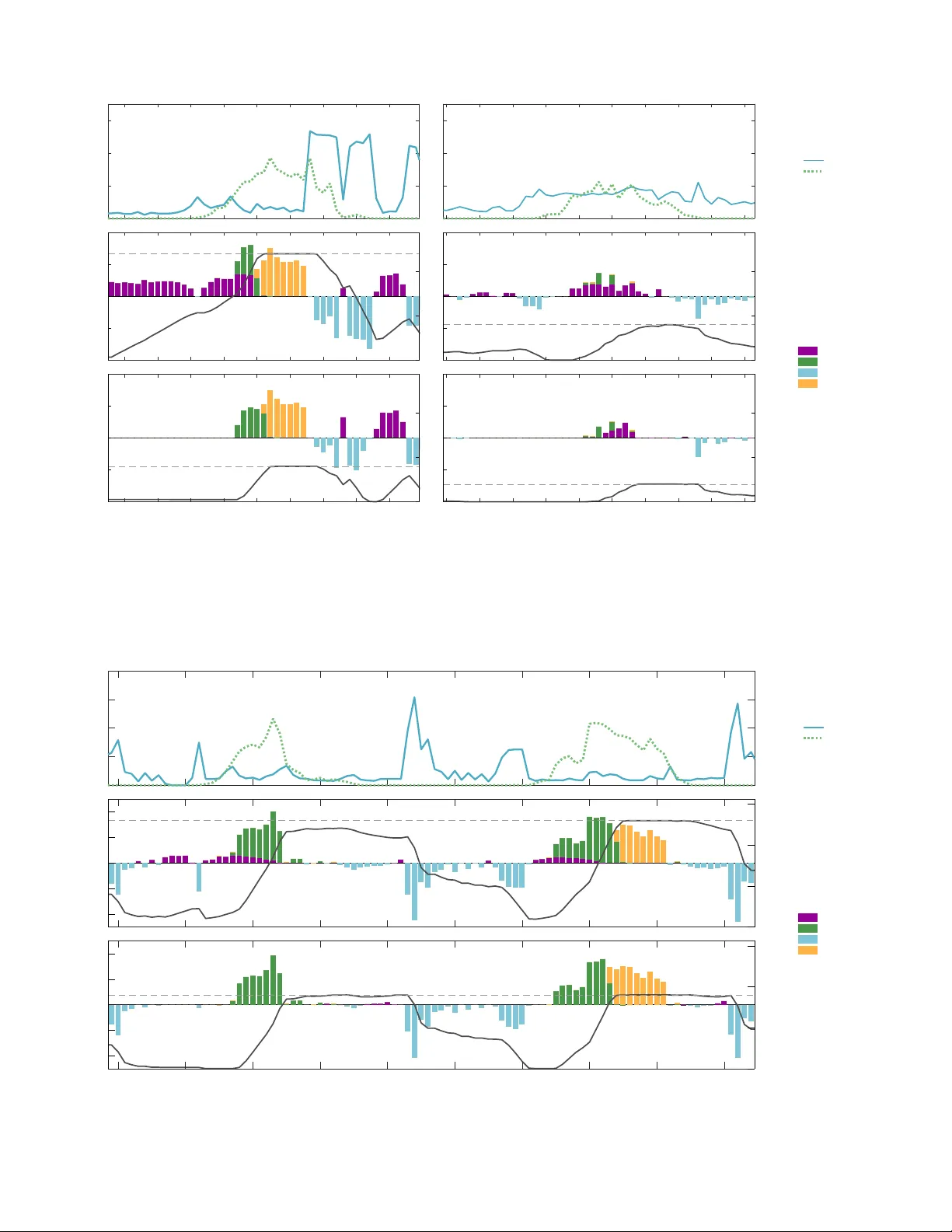
1 On Optimal Battery Sizing for Households P articipating in Demand-Side Management Schemes Matthias Pilz, Omar Ellabban, and Luluwah Al-F agih Abstract —The smart grid with its two-way communication and bi-directional power layers is a cornerstone in the combat against global warming. It allows for the large scale adoption of distrib uted (individually-owned) renewable ener gy resour ces such as solar photovoltaic systems. Their intermittency poses a threat to the stability of the grid which can be addr essed by the introduction of energy storage systems. Determining the optimal capacity of a battery has been an active area of resear ch in recent years. In this resear ch an in-depth analysis of the relation between optimal capacity , and demand and generation patterns is performed for households taking part in a community-wide demand-side management scheme. The scheme is based on a non-cooperative dynamic game approach in which participants compete f or the lo west electricity bill by scheduling their energy storage systems. The r esults are ev aluated based on self-consumption, the peak-to-av erage ratio of the aggregated load, and potential cost reductions. Furthermore, the difference between individually-owned batteries to a centralised community energy storage system serving the whole community is in vestigated. Index T erms —Smart Grid, Battery Scheduling, Game Theory , Optimal Sizing, Real Data, Self-Consumption I . I N T R O D U C T IO N Global average temperatures are rising dramatically (2016 being the warmest year e ver recorded [1]), causing a noticeable increase in natural disasters and en vironmental issues [2]. Thus it is imperativ e to in vestigate approaches that reduce greenhouse gas emissions and slow down climate change. Instead of burning fossil fuels to satisfy our energy needs, humans should make use of renew able energy resources such as solar and wind, which hav e a smaller carbon footprint. In order to guarantee a stable power grid, demand and generation hav e to be balanced at all times. This makes the inte gration of renewable resources a challenging task due to their inter - mittent nature. The advent of the smart grid, a technologically advanced power grid, is a possible solution to this problem. It combines the legacy power grid with a communication layer, effecti vely connecting all the grid participants. Through this additional infrastructure energy consumption can be managed. More specifically , in this research, the functionality to exchange data between individual households is being used to schedule ener gy storage installations such that the grid stability The authors want to thank Hamad Bin Khalifa University and the Doctoral T raining Alliance (DT A) Energy for their support. M. Pilz is with the School of Computer Science & Mathematics at Kingston Univ ersity London in Kingston upon Thames, UK. O. Ellabban is with Iberdrola Innov ation Middle East, Qatar Science & T echnology Park, Doha, Qatar . L. Al-Fagih is with the Division of Engineering Management and Decision Sciences in the College of Science and Engineering at Hamad Bin Khalifa Univ ersity , Qatar. is guaranteed ev en though a considerable amount of demand is served from solar power generation facilities. A key element to achiev e a high self-consumption rate of solar energy , i.e. the ratio between the consumed solar energy to the actual demand, is the utilisation of energy storage. V arious research studies are concerned with energy storage management [3]–[8]. Luthander et al. [6] present a case study of 21 Swedish households with a focus on comparing indi vidually-owned batteries to a centralised storage solution. In order to reach a certain le vel of self-consumption the centralised storage capacity is considerably smaller than the aggregated capacity of individually-o wned batteries. The study in [7] is concerned with optimising the usage of a giv en photov oltaic-battery system. It in vestigates a number of different optimisation objectiv es and shows how these af fect the e ventual charging patterns of a household for two exemplary days. In contrast to their approach, Reference [8] makes use of a game-theoretic approach in which households schedule their indi vidually- owned batteries with the goal to minimise their respective electricity bills. They perform simulations over the period of an entire year to allow for statistical analysis of the results. One interesting question is: What is the optimal capac- ity of a battery? [9]–[11]. Reference [11] focuses on the influence of different tariff schemes on the optimal battery size, whereas [10] de velops a decision-making tool which supports users that are in vesting in photo voltaic and battery systems. Recently , Huang et al. [9] dev eloped an algorithm to determine the optimal size of a battery with respect to the achiev able self-consumption. This research builds on their approach and dev elops a deeper understanding of the relation between demand and generation patterns, and the optimal battery capacity . The main contributions of this research are as follows: (1) Based on seasonal and yearly simulations of households with real consumption and generation data, this research provides an in-depth insight on ho w optimal sizing of batteries depends not only on aggre gated statistics b ut also on the specific temporal patterns that characterise individual households. (2) T wo dif ferent battery scheduling algorithms are compared in terms of three metrics: (i) Self-consumption of solar energy , (ii) Peak-to-average ratio of the aggregated load as an indicator for grid stability , and (iii) Potential cost reductions due to the introduction of electricity storage systems. (3) This research compares the optimal sizing for a cen- tralised storage facility with individually-o wned batteries 2 and analyses their effect on the same metrics as men- tioned above. This paper is organised as follo ws. In Section II, the neigh- bourhood model is presented. This includes a brief summary of the models for the storage and generation systems, general definitions of demand and load, as well as the role of the utility company . Furthermore, the underlying battery schedul- ing game is explained. Section III introduces the dataset and simulation parameters before summarising, analysing, and discussing the results. The paper is concluded in Section IV. I I . S Y S T E M M O D E L A N D S C H E D U L I N G O B J E C T I V E S In this section, the model for the community and its partic- ipants is briefly summarised. For a more detailed description of the setup the reader is kindly referred to [8]. A. Neighbourhood Consider a neighbourhood of M households that is modeled as a set M . Each of the households m ∈ M is equipped with a smart meter , an individually-o wned battery , and a photov oltaic (PV) system that con verts solar energy into electricity . The smart meters hav e the capability to measure consumption and generation data over equidistant time intervals t ∈ T . A day is split into T intervals. Furthermore, the smart meters are able to exchange data through wireless communications. B. Households A detailed battery model is employed. It includes the charging and discharging efficienc y ( η + , η − ) of the storage device, self-dischar ging at a rate of ¯ ρ in case the battery is idle, and also limits on how much can be char ged or discharged ( ρ + , ρ − ) during a particular interval t ∈ T . Furthermore, the con version efficiency η in v of the DC/A C power electronics con verter is considered. The main equations characterising the battery model are as follows, more details are presented in [8]: S O C t +1 = S O C t + η in v η + a t + charging (1a) S O C t +1 = S O C t + a t − / η inv η − discharging (1b) 0 ≤ a t + < ρ + charging rate (1c) ρ − < a t − ≤ 0 discharging rate (1d) SOC min ≤ SOC t ≤ SOC max limited SOC , (1e) where SOC is the state-of-charge of the battery , a t + and a t − are the char ging and discharging amount in interval t , respectiv ely , and SOC min and SOC max giv e the lo wer and upper bound of the SOC. Each household is equipped with a solar PV system for local consumption. The PV systems v ary in size according to the dataset described in Section III-A. The solar energy generated locally w t m is always taken into account before making a scheduling decision for a specific interval t . This means that if av ailable, the ener gy from the PV system is used to fulfil the demand ¯ d t m of a household. Furthermore, if the solar PV generation exceeds the demand it is stored in the local battery (if possible). Note that charging the battery from the solar PV system does not require DC/A C conv ersion, whereas it needs to be con verted to AC before it is being used to fulfil demand. Therefore, the net-demand of a household m ∈ M at time interval t ∈ T can be written as d t m = ¯ d t m − w t m . (2) Then the load l t on the electricity grid, i.e. the amount of electricity that is provided by the utility company , can be written as l t m = d t m + a t m . (3) C. Utility Company All the community households are supplied by one network distribution company , which incentivises each household in- dividually to reduce their energy consumption during peak hours. A billing strategy which calculates a unit energy price per interval t based on the aggregated load of all customers is giv en by p t = c 2 · y t + c 1 · y t + c 0 , (4) where y t is the aggregated load of all users at interval t and c 2 > 0 , c 1 , c 0 ≥ 0 are constants. As a consequence the energy bill for a particular day of an individual household can be calculated as: b m = X t l t m · p t . (5) D. Game Scheduling and Self-Consumption Constraint The batteries of the households are scheduled based on a dynamic game which is played between the individual households. The objectiv e of the players/households is to minimise their individual electricity bill (5). They act ratio- nally and in a selfish manner . In the follo wing section, two approaches are differentiated. The first approach is identical to the one proposed by [8] and will be called “Game-Theoretic Scheduling” (GTS). The game is played for an upcoming day based on forecasts for demand and generation. The second approach indroduces an additional constraint to the GTS. Whenever the rene wable PV generated energy is expected to be higher than the demand for an upcoming interval, charging the battery from the grid is prohibited. The idea behind this is to maximise the self-consumption rate of the PV system. This approach will be referred to as “Game- Theoretic Scheduling with Constraint” (GTSWC). I I I . S I M U L A T I O N S W I T H T H E A U S G R I D D AT A S E T In this section, the Ausgrid dataset and further simulation details are presented. Then the ev aluation metrics are defined. Eventually , the simulation results are analysed and discussed. A. Data, Simulation Details, and Metrics For all the following simulations the real-world “ Ausgrid” dataset [12] is being used. This dataset has been collected half hourly , i.e. T = 48 interv als, from 300 indi vidual homes in the Ausgrid’ s electricity network (Ne w South W ales, Australia) ov er three years (2010-2013). All of the homes are equipped with solar PV systems between 1.05 kWp and 9.99 kWp. The 3 T ABLE I Season Definitions . season period winter 01 / 07 / 2010 − 28 / 09 / 2010 spring 01 / 10 / 2010 − 29 / 12 / 2010 summer 01 / 01 / 2011 − 31 / 03 / 2011 autumn 01 / 04 / 2011 − 29 / 06 / 2011 period between July 2010 and June 2011 has been split into four seasons as shown in T ab . I. This is done such that each individual season spans exactly 90 days. A clean version of the Ausgrid dataset, which contains M = 54 households is considered in this research. Please refer to [13, Chapter 2] and [14] for a thorough analysis of the complete dataset. The consumption and generation data are used as an input to the day-ahead scheduling mechanism described in Section II-D. This means they are treated as forecasted data and throughout this study no forecasting errors are considered. The optimal battery size for each household is determined following a process reported by Huang et al. [9]. As there are two scheduling approaches (GTS and GTSWC), this is done twice for each season and also independently for an entire year resulting in lists of optimal battery capacities for each household. After that one run for each approach and season in which the households are equipped with their individually determined optimal battery size has been performed. For comparison of the outcomes, the following three metrics are being used: (i) The percentage increase in self-consumption by the introduction of the battery , (ii) The cost reduction due to the introduction of the battery according to the billing function shown in Section II-C, and (iii) The peak-to-average ratio (P AR) of the aggregated load of all the households, i.e. P AR = T · max m P t l t m P n P τ l τ n . (6) B. Optimal Battery Sizing Results and Discussion In order to determine the optimal battery size, the process described in [9] has been followed. T o do so, simulations are performed with different battery sizes for each household (per season and yearly) using both scheduling approaches. Battery capacities are in the range between 1.0 kWh and 27.0 kWh. The upper limit would equal an installation of two T esla Po werwall2 batteries [15]. F or each set of parameters, the ‘effecti veness’ of the electricity storage is computed. The effecti veness is defined by the notion of how much the self- consumption of a household is increased per kWh of installed capacity: effecti veness = sc n − sc 1 n , (7) where sc n is the self-consumption achiev ed by utilising stor- age of size n kWh. The maximum of this effecti veness is the sought after optimal battery size. An example for these steps is shown in Fig. 1 for a randomly selected house and season. The optimal battery size for each player ov er the course of an entire year for the two approaches (game-theoretic schedul- ing with and without self-consumption constraint, cf. Sec- tion II-D) is shown in Fig. 2. Furthermore, Fig. 2 also reports 30 35 40 45 50 55 self-consumption (%) GTS GTSWC 0 5 10 15 20 25 battery capacity (kWh) 0 0.5 1 1.5 effectiveness Fig. 1. Optimal sizing considerations . The self-consumption and the resulting effecti veness of an exemplary household are plotted over the battery size. The two vertical lines indicate the maximum of the effecti veness for the GTS and GTSWC approach and therefore the optimal size of the energy storage installation, respectiv ely . T ABLE II Self-consumption impr ovements . T H E M E D IA N I M PR OV EM E N T ( OV E R A L L H O US E H O LD S ) O F T H E S E LF - C O NS U M PT I O N D U E T O T H E I N T RO D UC T I ON O F O P T IM A L L Y S I Z ED B A T T E RI E S I S S H OW N . T H E S I M UL ATI O N S F O R E AC H C O LU M N W E R E P E R FO R M E D I N DE P E ND E N T L Y . winter spring summer autumn yearly GTS 11 . 4% 17 . 8% 10 . 0% 11 . 3% 11 . 6% GTSWC 12 . 1% 17 . 0% 10 . 7% 12 . 2% 12 . 5% the av erage results per season ov er all the 54 in vestigated households. Overall, the optimal size for the GTSWC scenario does not e xceed the GTS optimal battery size for any player and season. Houshold 4 sho ws the smallest dif ference between the two scenarios. All the capacities are the same except for summer where they differ by 1 kWh. The lar gest dif ference between the optimal battery size as determined for the two approaches of a particular season is found in household 14 (summer). Here the difference is 8 kWh (cf. Fig. 1). The largest difference between the optimal battery size for two seasons and the same approach is seen in household 52 (winter: 11 kWh, summer: 3 kWh). In Section III-C, these households are inv estigated in particular to understand ho w their battery usage patterns lead to the respectiv e results. 1) Self-Consumption: The solar PV self-consumption rate of a household is defined as the ratio between the solar energy being used and its demand. This includes a direct part which is consumed immediately and an indirect part used to charge the battery when the PV system generation exceeds the local demand. In the follo wing, the increase in self-consumption due to the introduction of an optimally sized battery for both the GTS and GTSWC scenario is analysed. The seasonal results for the self-consumption can be found in Fig. 3. Explicit improvements are reported in T ab . II. It becomes clear that ev en with different optimal battery sizes for the GTS and GTSWC approach the median 4 0 5 10 15 winter spring summer autumn 0 5 10 15 yearly 0 5 10 15 optimal battery size (kWh) GTS 5 10 15 20 25 30 35 40 45 50 household ID 0 5 10 15 optimal battery size (kWh) GTSWC Fig. 2. Optimal battery sizes . The results are obtained through a process as described in [9].Battery capacities between 1 and 27 kWh were analysed. The optimal battery sizes for the individual households from simulation runs over the period of an entire year are reported. Furthermore, statistical results for these simulations as well as independent seasonal simulations are shown. winter spring summer autumn yearly 0 10 20 30 40 50 60 70 80 90 100 self-consumption (%) GTSWC GTS reference Fig. 3. Self-consumption analysis . Statistical results for the self-consumption rates are shown for all seasons and an entire year . For each period, the refer- ence case in which no storage is av ailable is compared with a configuration that includes the optimally sized batteries for each individual household for both the GTS and the GTSWC approach. improv ement in self-consumption is similar . The result was to be e xpected as the additional constraint in GTSWC is particularly designed to place further emphasis on the increase of self-consumption. The spread around the median self-consumption approximately doubles when comparing the results with the reference case in which no batteries are present. This is due to the fact that some households benefit more than others from the introduction of a battery . There are many factors that play a role for this such as the aggregated solar production, the aggregated demand, and also the temporal patterns of production and demand. For example: Household 14 improves its self-consumption by 12 . 2% during the summer, while household 26 (with similar aggregated consumption and PV peak production) improv es its self-consumption by 1 . 5% . Household 13, which has less aggregated demand than the two houses mentioned before and higher aggregated solar production, improves its self-consumption by 37 . 9% . A more detailed analysis of these households and how these differences are related to their demand patterns will be analysed in Section III-C. In general 1 , households that gain considerably at GTS also do so at GTSWC and vice versa. The av erage absolute dif ference of the self-consumption improvements between GTS and GTSWC for each household individually is < 1 . 4% . 2) P AR values: The peak-to-average ratio (P AR) of the aggregated load (6) is an indicator for the stability of the grid [16]. A value close to 1.0, i.e. a flat load profile, is preferred by a utility company as this allo ws them to sav e in vestment costs for fast-ramping energy production installations. P AR v alues are calculated for a period of one day . A statistical analysis for the 90 days that comprise each season is shown in Fig. 4. Overall, considerable improvements of the P AR value are achiev ed. The GTS approach leads to better P AR reductions than the GTSWC approach in both the median values and also the smaller spread around these. 3) Cost Reduction: As seen in Section II-C, the cost function (4) depends on the aggregated load. Thus the price per unit of electricity changes for each half hour interval. When calculating the overall bill for each household with and without battery , it can be observed that it is decreasing in both approaches. The relati ve cost reduction of the electricity bill due to the introduction of an optimally sized battery is shown in Fig. 5. Overall, the introduction of energy storage leads to a considerable amount of savings from the electricity 1 Explicit results for this statement are not shown due to lack of space. 5 winter spring summer autumn yearly 1 1.2 1.4 1.6 1.8 2 2.2 2.4 2.6 2.8 3 peak-to-average ratio of aggregated load () GTSWC GTS reference Fig. 4. P eak-to-average ratio (P AR) of the aggre gated load. A statistical analysis of the achie ved daily P AR v alues over the respecti ve seasons is shown. For each period, the reference case in which no storage is available is compared with a configuration that includes the optimally sized batteries for each individual household for both the GTS and the GTSWC approach. winter spring summer autumn yearly 0 10 20 30 40 50 60 70 80 90 100 cost reduction (%) GTSWC GTS Fig. 5. Cost reductions . Statistical analysis of the amount of savings from the electricity bill over various billing periods is presented for the GTS and the GTSWC approach. The calculation of the unit energy price depends on the aggregated load as introduced in (4). bill in both cases (GTS and GTSWC). The increase of self- consumption can directly be translated in a decrease of energy requested from the grid which in turn decreases the bill. As seen in the previous section (cf. Section III-B1), the achiev ed improv ements in self-consumption are similar for the two approaches. This means this fact alone cannot explain the higher savings from GTS compared to GTSWC. The second factor that plays a role is the more ef fectiv e P AR reduction observed for the GTS approach (cf. Section III-B2). Due to the quadratic relation between the aggreg ated load and the price per unit of electricity , consumption during peak times is billed highly . The spread around the median v alues for both approaches is similar . C. Analysis of Battery Usage P atterns While the aggregated demand of a household and the size of their installed solar panel can give a rough estimate for the optimal battery size, it remains important to look at the actual demand and generation patterns. In Section III-B1 it was visible that tw o households with similar aggregated demand and peak PV output benefited dif ferently from their storage installation. In order to understand this difference, Fig. 6 sho ws the demand and generation profile for a randomly chosen day together with the detailed battery usage for these two households. The demand of household 14 is lo w during the time when solar is av ailable and peaks shortly afterwards, whereas the demand of household 26 is rather e venly dis- tributed throughout the day . Household 26 is a prime example of a user that has a high percentage of non-curtailed solar energy even without a battery installation and cannot gain much through the utilisation of storage. Consequently , the optimal battery sizing algorithm determines a belo w-average optimal storage capacity for this household. In contrast to this, the battery of household 14 is optimally sized at an abov e- av erage capacity . W ithout storage a lot of the solar ener gy is curtailed due to the lack of demand at the particular time of generation. Since there is a peak in demand in the later hours, the self-consumption can be increased due to the storage capability . The left-hand plots in Fig. 6 also give insight into the differences between the GTS and GTSWC approach. During the fist half of the day , the GTS algorithm charges the battery from the grid, whereas the GTSWC anticipates the solar generation and thus restricts charging from the grid. The first two peaks in demand (cf. between interval 2144 and 2152) can then be met by previously saved electricity . In anticipation of another peak in demand at the end of the day , both algorithms charge the battery and are able to flatten the load curve considerably . It becomes clear that because no more solar production is to be e xpected during this time there are no constraints on char ging the battery from the grid and both algorithms behave similarly . Fig. 7 shows the demand and generation pattern together with the battery usage for two consecutive days of household 13. This household was chosen as it has the highest benefit during this particular season from installing an optimal battery size. A similar profile for the demand and generation as seen for household 14 in Fig. 6 can be observed. The ev en higher improv ement in self-consumption for this case stem from the more pronounced asynchronisation between solar generation and actual demand. Also, this household is equipped with a bigger solar panel. This section is concluded by analysing the demand and generation profile (Fig. 8) for the household that showed the biggest dif ference in optimal battery size between two seasons, i.e. household 52. For winter 2010 the optimal capacity is determined to be 11 kWh while in summer 2011 it is 3 kWh. 6 0 1 2 3 electricity (kWh) household 14 GTS -1 0 1 electricity (kWh) - bars 0 5 10 GTSWC 2115 2120 2125 2130 2135 2140 2145 2150 2155 #interval -1 0 1 electricity (kWh) - bars 0 5 10 0 1 2 3 household 26 demand generation GTS -1 0 1 0 5 10 SOC (kWh) - line grid charge solar charge discharge solar curtailed GTSWC 2785 2790 2795 2800 2805 2810 2815 2820 2825 2830 #interval -1 0 1 0 5 10 SOC (kWh) - line Fig. 6. Demand, generation, battery usage . The demand and generation profiles of household 14 (left) and household 26 (right) for representative days are shown. Furthermore, the specific battery usage based on the GTS and GTSWC approach are presented. For these four plots, the left hand axes represent the electricity values for the bars, while the right hand axes indicate the state of charge (SOC) of the respectiv e battery . The dotted line indicates the optimal battery size for the repsecti ve household. For this particular day household 14 improves their self-consumption by 6 . 0% / 10 . 4% through the GTS / GTSWC approach, respectiv ely . Household 26 improves their self-consumption by 2 . 7% for both approaches. 0 1 2 3 4 electricity (kWh) household 13 demand generation GTS -2 -1 0 1 2 electricity (kWh) - bars 0 5 10 15 SOC (kWh) - line grid charge solar charge discharge solar curtailed GTSWC 2210 2220 2230 2240 2250 2260 2270 2280 2290 2300 #interval -2 -1 0 1 2 electricity (kWh) - bars 0 5 10 15 SOC (kWh) - line Fig. 7. Demand, generation, battery usage . The demand and generation profiles of household 13 for two representative days are shown. Furthermore, the specific battery usage based on the GTS and GTSWC approach are presented. For the lower two plots, the left hand axes represent the electricity values for the bars, while the right hand axes indicate the state of charge (SOC) of the respectiv e battery . 7 0 1 2 3 electricity (kWh) household 52 winter 2600 2610 2620 2630 2640 2650 2660 2670 2680 #interval 0 1 2 3 electricity (kWh) summer demand generation Fig. 8. Demand and generation for two seasons . The demand and PV generation of household 52 for two consecutive representativ e days of winter 2010 and summer 2010 are shown. D. Centr alised vs. Decentralised Storage Systems In all the previous simulations, each household was in possession of an indi vidual battery of different size. W ithin this section, a scenario that has a single battery to serve the community is in vestigated. For a reasonable comparison, the efficienc y of the battery and the DC/A C power electronics con- verter equal the values used before. Furthermore, the maximal charging and discharging rates were scaled up by the number of households. Firstly , full-year simulations with battery sizes varying between 10 kWh and 370 kWh were performed. Follo wing the optimal sizing procedure by [9], the optimal battery capacity for both the GTS and GTSWC approach were calculated to be 270 kWh and 90 kWh, respectiv ely . For these optimal sizes, the self-consumption, the peak-to-average ratio (P AR) of the aggregated load of all households, and the cost reduction according to the pricing function (5) are analysed. The results are shown together with the respectiv e results from yearly simulations of individually-o wned batteries in Fig. 9. The centralised optimal battery sizes are approximately 10% and 50% smaller than the aggregated capacities of the decentralised batteries for the GTS and GTSWC approach, re- spectiv ely . This is in agreement with a previous study reported by Luthander et al . [6]. In Section III-C, it was shown that in case of asynchronous demand and generation profiles, a large battery is most beneficial, while in the opposite case a small battery is sufficient. When looking at the centralised battery , note that it is scheduled according to the aggregated demand and generation of all the households. An av eraging effect for the demand profiles occurs, which makes the asynchronous case less likely and e ventually leads to a smaller optimal storage capacity . The PV self-consumption reaches a com- parable le vel to the decentralised simulations. Compared to the median self-consumption of all the households, a scenario with a centralised battery improv es the self-consumption by approximately 5% for both the GTS and GTSWC approach. When analysing the daily P AR v alues, it becomes clear that the community batteries perform worse both in terms of the achiev ed median values and also the spread around it. From the utility companies’ perspectiv e this is a unfav ourable result. Their most desirable objectiv e is to reduce the P AR value as it guarantees grid stability and financial benefits in the long run. The right-most panel in Fig. 9 shows the results for the cost reduction for both approaches comparing the centralised and decentralised neighbourhoods. For the GTS approach the centralised community achieves an approximately 5% higher cost reduction, while for the GTSWC approach the cost reduction is reduced by approximately 5% compared to the median cost reduction of all the households with individually- owned batteries. Both results for the centralised battery are within the interquartile range of the respective analysis for the decentralised system. I V . C O N C LU S I O N S In this paper , a community of households that take part in a demand-side management scheme is analysed. The focus was to gain deeper understanding of optimal battery sizing. Both the characteristics that lead to the optimal battery size determi- nation as well as the effect this optimal size has on solar pho- tov oltaic (PV) self-consumption ratio, grid stability/security , and cost reductions for the users has been in vestigated. A key insight is that the temporal patterns of consumption and generation impact the battery sizing critically . This means battery sizing which is soley based on aggregated data might lead to unfa vourable results. Households which benefit most from installing a energy storage system are those where the peak-production and peak-consumption is asynchronous, i.e. during different intervals of the day . Furthermore, two different approaches for the demand-side management scheme were compared. Game-theoretic schedul- ing (GTS) is based on the ideas presented in [8]. Here the main objectiv e of the individual households is to minimise their electricity bills. The second approach introduced an addi- tional constraint to the GTS which puts PV self-consumption before the minimisation of the costs. As a result it lead to considerably smaller optimal battery sizes. The drawback of the more constrained approach are the larger peak-to-average ratio of the aggreg ated load, i.e. higher costs for the utility company to guarantee stability of the grid. In terms of costs a trade-off is achieved: On the one hand, the initial inv estments are smaller for GTSWC due to the smaller battery sizes. On the other hand, the cost reduction of f the electricity bill are less beneficial. The final part of the paper compared individually-o wned batteries with a scenario that incl udes a utility sized centralised storage system. The optimal battery size determined for the centralised system is smaller due to less pronounced asyn- chrony of the aggregated demand to the solar PV production. V . A C K N OW L E D G E M E N T S The authors would like to thank Jean-Christophe Nebel for useful comments and valuable discussions. 8 GTS GTSWC 0 50 100 150 200 250 300 aggregated battery size (kWh) GTS GTSWC 0 20 40 60 80 100 self-consumption (%) GTS GTSWC 1 1.5 2 2.5 3 PAR values () GTS GTSWC 0 20 40 60 80 100 cost reduction (%) individual community individual community Fig. 9. Comparison between centralised and decentralised approac h . The aggregated optimal battery sizes for the GTS and GTSWC approach in case of a single centralised battery and individually-o wned decentralised batteries are shown. Furthermore the three metrics: self-consumption, peak-to-average ratio (P AR) of the aggregated load, and cost reduction are investigated for simulations based on these optimally sized storage installations. All simulations are performed over the period of an entire year, i.e. winter 2010 to autumn 2011. R E F E R E N C E S [1] N ASA, “Global Climate Change Facts - V ital Signs, ” 2019. [Online]. A vailable: https://climate.nasa.gov/vital- signs/global- temperature/ [2] ——, “Global Climate Change Facts - Effects, ” 2019. [Online]. A vail- able: https://climate.nasa.gov/ef fects/ [3] H. M. Soliman and A. Leon-Garcia, “Game-Theoretic Demand-Side Management With Storage Devices for the Future Smart Grid, ” IEEE T ransactions on Smart Grid , vol. 5, no. 3, pp. 1475–1485, 2014. [4] H. K. Nguyen, J. B. Song, and Z. Han, “Distributed Demand Side Management with Energy Storage in Smart Grid, ” IEEE T ransactions on P arallel and Distributed Systems , vol. 26, no. 12, pp. 3346–3357, 2015. [5] T . Y . Li and M. Dong, “Real-Time Residential-Side Joint Energy Stor- age Management and Load Scheduling With Renewable Integration, ” IEEE T ransactions on Smart Grid , vol. 9, no. 1, pp. 283–298, 2018. [6] R. Luthander , D. Lingfors, J. Munkhammar , and J. Wid ´ en, “Self- Consumption Enhancement of Residential Photov oltaics W ith Battery Storage and Electric V ehicles in Communities, ” Pr oc. of eceee summer study on energy efficiency , pp. 991–1002, 2015. [7] J. Li and M. A. Danzer, “Optimal Charge Control Strategies for Stationary Photov oltaic Battery Systems, ” Journal of P ower Sources , vol. 258, pp. 365–373, 2014. [8] M. Pilz and L. Al-Fagih, “A Dynamic Game Approach for Demand- Side Management: Scheduling Energy Storage With Forecasting Er- rors, ” Dynamic Games and Applications: Dynamic Games for Smart Ener gy Systems , 2019. [9] J. Huang, J. Boland, W . Liu, C. Xu, and H. Zang, “A Decision-Making T ool for Determination of Storage Capacity in Grid-Connected PV Systems, ” Renewable Energy , vol. 128, pp. 299–304, 2018. [10] R. Khalilpour and A. V assallo, “Planning and Operation Scheduling of PV -Battery Systems: A Novel Methodology , ” Renewable and Sustain- able Energy Reviews , vol. 53, pp. 194–208, 2016. [11] O. T alent and H. Du, “Optimal Sizing and Energy Scheduling of Photov oltaic-Battery Systems Under Different T ariff Structures, ” Re- newable Energy , vol. 129, pp. 513–526, 2018. [12] Ausgrid, “Solar Home Electricity Data 2010-2013, ” 2019. [Online]. A vailable: https://www .ausgrid.com.au/Industry/ Innov ation- and- research/Data- to- share/Solar- home- electricity- data [13] E. L. Ratnam, “Balancing Distributor and Customer Benefits of Battery Storage Co-Located With Solar PV, ” Ph.D. dissertation, 2016. [14] O. Ellabban and A. Alassi, “Integrated Economic Adoption Model for Residential Grid-Connected Photovoltaic Systems: An Australian Case Study, ” Energy Reports , vol. 5, pp. 310–326, 2019. [15] T esla, “T esla Powerwall 2, ” 2017. [Online]. A vailable: https://www . tesla.com/en GB/powerwall [16] I. S. Bayram, M. Z. Shakir , M. Abdallah, and K. Qaraqe, “A Surve y on Energy Trading in Smart Grid, ” 2014 IEEE Global Confer ence on Signal and Information Processing , pp. 258–262, 2014.