Design of Pulse Shapes Based on Sampling with Gaussian Prefilter

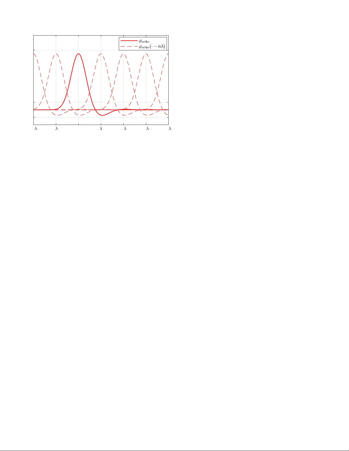
Design of Pulse Shapes Based on Sampling with Gaussian Prefilter Edwin Hammerich Ministry of Defence, 95030 Hof, Germany E-mail: edwin.ham merich@ieee.org Abstract —T wo new pulse shapes for co mmunications are presented. The first p u lse shape generates a set of p ulses without intersymbol interfer ence (ISI) or ISI-free fo r short. In the neighborhood of t h e origin it is similar in shape to the classical cardinal sine function but is of exponential decay at infin ity . This pu lse sh ape is identical to the in terpolating function of a generalized sampling th eorem with Gaussian p refilter . The second pul se shape is obtain ed from the first pulse shape by spectral factorization. Besid es being also of exponenti al decay at infinity , it has a causal app earance since it is of superexponential decay for negativ e times. It is closely related to the orthonormal generating fun cti on considered earlier by Unser in the context of sh ift-inv ariant spaces. Th is pu lse shape is not IS I-free but it generates a set of orthonormal pulses. The second pulse shape may also b e u sed to defi ne a recei ve matched filter so that at the filter outp ut the IS I-free pulses of the fi rst kind are recov ered. I . I N T RO D U C T I O N Unser [ 1 ] extend ed the standard samplin g parad ig m to the representatio n or e ven approximation of function s by elemen ts of shift-inv ariant fun c tion spaces. These function spaces are defined by a generatin g function ϕ , which has to satisfy certain condition s. By on e of them, the partition of unity co ndition, Gaussian fun ctions are actually pr ecluded fro m b eing used as generato r s. I n [ 2] it was su b stantiated that Gaussian fu nctions still cou ld b e useful ge n erators. Co n sequently , following [1, T ab . 1], the interpolatin g generatin g fun c tion and th e du al generating functio n have been compu ted for a Gaussian g ener- ator in [2]. Th e compu tation of the cor respond in g orthon o rmal generating functio n, ϕ ortho , is accom plished in Section III of the present pap er . Rather than extracting the squ are ro ot as suggested in [1], ou r ap proach is based on spectral factoriza - tion and leads, intere sting ly enoug h, to expressions in terms of q -analo gs [3]. As an applicatio n, two new pu lse shap es are propo sed an d d iscussed in Section IV. The following notations and co n ventions are ad opted: L 2 ( R ) is the space of square- integrable functio ns (o r fin ite- energy signals) f : R → C ∪ {∞} with inner product h f 1 , f 2 i = R ∞ −∞ f 1 ( x ) f 2 ( x ) d x an d no rm k f k = h f , f i 1 / 2 . For the F ourier transform we use the definition ˆ f ( ω ) = (2 π ) − 1 / 2 R ∞ −∞ e − i ω x f ( x ) d x , wher e x denotes time and ω angular frequ ency . ℓ 2 ( Z ) is the space of square- summable, complex-valued sequences indexed by th e in tegers. Fina lly , δ n = 0 , n ∈ Z \ { 0 } , an d δ 0 = 1 . I I . S A M P L I N G I N S H I F T - I N V A R I A N T S PAC E S A N D L O C A L I Z A T I O N S PAC E S R E V I S I T E D The purpo se of the p resent section is to motivate the pu lse shapes presented in Section IV. T o this end, we gi ve a br ief overview of samp lin g in shift-inv ariant spaces and localization spaces with an emphasis on those spaces defined by a Gaussian generato r o r a Gau ssian prefilter respectively . Suppose that ϕ ∈ L 2 ( R ) is a con tin uous fun ction satisfying ϕ ( x ) = O ( | x | − 1 − ǫ ) as x → ± ∞ for som e ǫ > 0 an d for any λ > 0 the sy stem of functions { ϕ ( · − nλ ); n ∈ Z } forms a Riesz b asis in L 2 ( R ) . Furthermo re, suppose th a t for any λ > 0 ∞ X n = −∞ ϕ ( nλ )e − i nλω 6 = 0 , ω ∈ R . (1) The shift-inv ariant space V λ ( ϕ ) is the sub space o f L 2 ( R ) defined as V λ ( ϕ ) = ( f ; f ( x ) = X n ∈ Z c n ϕ ( x − nλ ) , c ∈ ℓ 2 ( Z ) ) . (2) Then, th e following sampling theorem applies. Theor em 1: For any λ > 0 an d f ∈ V λ ( ϕ ) it holds that f ( x ) = X n ∈ Z f ( nλ ) ϕ int ( x − nλ ) , x ∈ R , (3) where the interpolating functio n ϕ int ∈ V λ ( ϕ ) is giv en by ˆ ϕ int ( ω ) = ˆ ϕ ( ω ) P n ∈ Z ϕ ( nλ )e − i nλω = ˆ ϕ ( ω ) Λ √ 2 π P k ∈ Z ˆ ϕ ( ω + k Λ ) , Λ = 2 π λ . (4) This theorem is due to W alter [4], who origin a lly proved it fo r orthon ormal bases { ϕ ( · − n ); n ∈ Z } . The theorem was later extended to Riesz bases by Un ser [1], who also considered alternative g enerating function s for V λ ( ϕ ) like ϕ int as above and ϕ ortho (see below). In an attem pt to retain the flav or of th e original Whittaker –K otelnikov–Shannon (WKS) sampling th eorem [ 5], in [6] prior to sampling a prefilter ( P ϕ f ) ( x ) = Z ∞ −∞ f ( y ) ϕ ( y − x ) d y (5) with prefilter function ϕ ∈ L 2 ( R ) has been applied to an arbitrary finite-en ergy signal f ∈ L 2 ( R ) . The so-called localization sp ace P ϕ = { g = P ϕ f ; f ∈ L 2 ( R ) } then corre sponds to the space of bandlim ited, finite-energy signals in the classical WKS samplin g theorem. Th e goal is to recover the filter output signal g = P ϕ f from sample values g ( nλ ) , n ∈ Z , either perfectly or at least with an ac c eptable error . T o this en d, th e au tocorrelatio n f unction Φ of ϕ , Φ = P ϕ ϕ ∈ P ϕ F ourie r ← → ˆ Φ( ω ) = √ 2 π | ˆ ϕ ( ω ) | 2 , (6) is n eeded. Th e (second) inter polating fun ction Φ int ∈ P ϕ is defined by its Fourier transfo rm ˆ Φ int ( ω ) = ˆ Φ( ω ) Λ √ 2 π P k ∈ Z ˆ Φ( ω + k Λ) , (7) where Λ is as in (4). Note th at because o f th e Riesz basis condition still imposed o n ϕ (see [6] f or the f u ll set of assumptions), which is equiv alent to the existence o f p ositi ve constants A and B (p ossibly dep e n ding on λ ) so that [7] 0 < A ≤ Λ ∞ X k = −∞ | ˆ ϕ ( ω + k Λ ) | 2 ≤ B < ∞ , ω ∈ R , (8) the den o minator in (7) never will vanish. W e remark that in general Φ int 6 = P ϕ ϕ int . I n the special ca se of a Gaussian prefilter function , ϕ ( x ) = 1 √ 2 π (1 /β ) e − x 2 2(1 /β ) 2 F ourie r ← → ˆ ϕ ( ω ) = 1 √ 2 π e − ω 2 2 β 2 , (9) where the par a meter β > 0 controls effective band width, the following gen eralized sampling theorem has been o b tained [2], [6]. Theor em 2: For any λ > 0 let the interpo lating function Φ int be d efined b y (7 ). T hen fo r any function g ∈ P ϕ , wh e re g = P ϕ f , f ∈ L 2 ( R ) , the functio n ˜ g gi ven by ˜ g ( x ) = X n ∈ Z g ( nλ )Φ int ( x − nλ ) , x ∈ R , (10) is aga in in P ϕ , it perfectly recon structs g at the sampling instants x n = nλ, n ∈ Z , and fo r all other x ∈ R th e squared relativ e erro r ( | g ( x ) − ˜ g ( x ) | / k f k ) 2 becomes sm a ll as soo n as λ ≤ 1 /β , th en decaying superexpo nentially to zero as λ → 0 . For the Gaussian p refilter function ϕ as given in ( 9 ) (which will be assumed for the rest of the pape r ) one has ˆ Φ int ( ω ) = λ √ 2 π e − i π τ ( ω / Λ) 2 √ − i τ ϑ 3 ( ω / Λ , τ ) , (11) where ϑ 3 ( z , τ ) = 1 √ − i τ ∞ X n = −∞ e − i π τ ( z + n ) 2 (12) is a Jacobi th eta fu nction [ 8] with par ameter τ g iv en by τ = i( λβ ) 2 / (4 π ) . (13) By in version of the Fourier transform we ob tain after u se o f Jacobi’ s τ → − 1 / τ tran sformation th at [2], [ 9] Φ int ( x ) = i π τ ϑ ′ 1 (0 , − 1 /τ ) ϑ 1 ( x/λ, − 1 /τ ) sinh(i π τ x/λ ) , (14) where ϑ 1 ( z , τ ) = 2 P ∞ n =0 q ( n + 1 2 ) 2 ( − 1) n sin[(2 n + 1) π z ] , q = e i π τ , ℑ ( τ ) > 0 , is ano ther the ta fu nction [8]. When λ ≤ 1 /β , it holds with high accuracy that Φ int ( x ) ≈ S 0 ( x ) , where [9] S 0 ( x ) , i τ sin( π x/λ ) sinh(i π τ x/λ ) , x ∈ R . (15) Note tha t in our co ntext i τ is alw ays a negative real number and that Φ int ( x ) decays exponentially to zero as x → ±∞ . Fig. 1 shows the interp olating f unction Φ int for β = 100 and λ = 1 / β ; actually , the appro ximation (15) fo r Φ int ( x ) has been used. I I I . S P E C T R A L F AC T O R I Z A T I O N O F T H E I N T E R P O L A T I N G F U N C T I O N W e start by comp iling a few pr e requisites [3]. Definition 1: For any a ∈ R and q ∈ C with | q | < 1 th e q -Pochh ammer symbo l ( a ; q ) n is d efined by ( a ; q ) n = (1 − a )(1 − aq ) · · · (1 − aq n − 1 ) , n = 1 , 2 , . . . , ( a ; q ) ∞ = lim n →∞ ( a ; q ) n , ( a ; q ) 0 = 1 . The following identities of Euler ho ld true fo r q ∈ C , | q | < 1 : 1 + ∞ X n =1 q 1 2 n ( n − 1) ( q ; q ) n z n = ∞ Y n =0 (1 + z q n ) , z ∈ C , (16) 1 + ∞ X n =1 z n ( q ; q ) n = ∞ Y n =0 (1 − z q n ) − 1 , z ∈ C , | z | < 1 . (17) Only Eq. (16) will be n eeded in th e pro of of th e next theor e m, where Jacobi’ s tr iple prod u ct id entity ∞ X n = −∞ q n 2 z n = ∞ Y n =1 (1 − q 2 n )(1 + q 2 n − 1 z − 1 )(1 + q 2 n − 1 z ) (18) will play a central role. In our case always q = e i π τ , (19) where param e ter τ is as in (13). The special q - Pochhamm er symbols ( q 2 ; q 2 ) n = n Y k =1 (1 − q 2 k ) , Q 0 , ( q 2 ; q 2 ) ∞ will occur f r equently . Theor em 3: For the functio n ϕ ortho ( x ) = 1 p ( q 2 ; q 2 ) ∞ ∞ X n =0 ( − 1) n q n ( q 2 ; q 2 ) n φ ( x − nλ ) , (20) where x ∈ R and φ ( x ) = β 1 / 2 π 1 / 4 e − x 2 2(1 /β ) 2 (21) is the Gaussian fun ction ϕ in (9 ) normalized to unit energy , i.e., R R | φ ( x ) | 2 d x = 1 , it holds that ˆ Φ int ( ω ) = √ 2 π | ˆ ϕ ortho ( ω ) | 2 , ω ∈ R . (22) Pr o of: Th e definition (11 ) of th e interpolatin g fun ction Φ int may be w r itten in the Fourier do main as ˆ Φ int ( ω ) = √ 2 π λ | ˆ ϕ ( ω ) | 2 √ − i τ ϑ 3 ( ω / Λ , τ ) . Then, E q. (22) become s | ˆ ϕ ortho ( ω ) | 2 = λ | ˆ ϕ ( ω ) | 2 √ − i τ ϑ 3 ( ω / Λ , τ ) . Since the theta function (12) has the second representa tio n [ 8 ] ϑ 3 ( x, τ ) = 1 + 2 ∞ X n =0 q n 2 cos(2 π nx ) = ∞ X n = −∞ q n 2 e 2 π i nx , we obtain by means of Eq. (18) , putting P ( z ) = ∞ Y n =1 (1 + q 2 n − 1 z − 1 ) and subsequen tly z = e 2 π i x , for ϑ 3 ( x, τ ) the factorization ϑ 3 ( x, τ ) = Q 1 / 2 0 P (e 2 π i x ) · Q 1 / 2 0 P (e 2 π i x ) , x ∈ R . Since th e fu nction x 7→ ϑ 3 ( x, τ ) is real-valued an d p ositiv ely lower boun ded on R so is the f unction x 7→ | P (e 2 π i x ) | . As a co n sequence, th e defin itio n o f ϕ ortho in the Fourier d o main by ˆ ϕ ortho ( ω ) = λ 1 2 ˆ ϕ ( ω ) ( − i τ ) 1 / 4 Q 1 / 2 0 P (e 2 π iω / Λ ) will result in a function ϕ ortho ∈ L 2 ( R ) satisfy ing Eq. (22). Now , we need to in vert the Fourier transfo rm. Sin ce x 7→ 1 /P (e 2 π i x ) is a b ound e d 1- periodic fun ction, it is in L 2 ([0 , 1)) and thus ha s a Fourier series expa n sion 1 /P (e 2 π i x ) = P ∞ n = −∞ a n e − 2 π i nx , a ∈ ℓ 2 ( Z ) , with the coefficients a n = Z 1 0 e 2 π i nx 1 P (e 2 π i x ) d x, n ∈ Z . (23) By inverse Fourie r tr ansform we now obtain (puttin g c = λ 1 / 2 ( − i τ ) − 1 / 4 Q − 1 / 2 0 ) that ϕ ortho ( x ) = c √ 2 π Z ∞ −∞ e i xω ˆ ϕ ( ω ) P (e 2 π i ω / Λ ) d ω = c ∞ X n = −∞ a n √ 2 π Z ∞ −∞ e i( x − nλ ) ω ˆ ϕ ( ω ) d ω = c ∞ X n = −∞ a n ϕ ( x − nλ ) = 1 Q 1 / 2 0 ∞ X n = −∞ a n φ ( x − nλ ) . The comp u tation of the coefficients ( 23) is carried out in the complex dom ain. Case n = − 1 , − 2 , . . . : After substitution in (2 3) of x by 1 − x we obtain a n = Z 1 0 e − 2 π i nx 1 P (e − 2 π i x ) d x = 1 2 π i I | z | =1 z − n − 1 P ( z − 1 ) d z , where integration in the contour integral is performe d coun- terclockwise aroun d th e unit circle. Since the integrand f unc- tion is analytic with in a neighbo rhood o f the closed unit disc, we obtain by means o f Cau c hy’ s integral theorem that a n = 0 , n = − 1 , − 2 , . . . Case n = 0 , 1 , . . . : Eq. (23) now direc tly y ields by transition to a contour integral that a n = 1 2 π i I | z | =1 z n − 1 P ( z ) d z = lim M →∞ 1 2 π i I | z | =1 z n − 1 P M ( z ) d z | {z } I M ( n ) , where P M ( z ) = M − 1 Y k =0 (1 + q 2 k +1 z − 1 ) , M = 1 , 2 , . . . , and the path of integration is same as bef ore. The integrand function in th e integral definin g I M ( n ) has simple p oles at z m = − q 2 m +1 , m = 0 , 1 , . . . , M − 1 , lying inside of th e unit circle. By means of th e theor e m of residues we obtain I M ( n ) = M − 1 X m =0 Res z m z n − 1 P M ( z ) , whence a n = lim M →∞ I M ( n ) = ∞ X m =0 Res z m z n − 1 P ( z ) . W e com p ute that Res z m z n − 1 P ( z ) = Res z m z n z P ( z ) = Res z m z n ( z − z m ) Q ∞ k =0 ,k 6 = m (1 + q 2 k +1 z − 1 ) = z n m Q ∞ k =0 ,k 6 = m (1 + q 2 k +1 z − 1 m ) = ( − q ) n q 2 mn ( q 2 ; q 2 ) ∞ Q m k =1 (1 − q − 2 k ) = ( − q ) n ( q 2 ; q 2 ) ∞ ( − 1) m q m ( m +1) ( q 2 n ) m Q m k =1 (1 − q 2 k ) , treating in the case of m = 0 the empty produ ct a s on e . After replacemen t of q in Eq. (16) w ith q 2 we get 1 + ∞ X m =1 q m ( m − 1) ( q 2 ; q 2 ) m z m = ∞ Y m =0 (1 + z q 2 m ) . Hence it holds that a n = ( − q ) n ( q 2 ; q 2 ) ∞ ∞ X m =0 q m ( m − 1) ( q 2 ; q 2 ) m ( − q 2( n +1) ) m = ( − q ) n ( q 2 ; q 2 ) ∞ ∞ Y m =0 (1 − q 2( n +1) q 2 m ) = ( − q ) n ( q 2 ; q 2 ) n , which conclud es the proo f o f Theor em 3. In Fig. 2, the fun ction ϕ ortho along with some of its translates is depicted fo r band width parameter β = 100 and λ = 3 /β . Pr o position 1: The function φ in (21) has for x ∈ R the representatio n φ ( x ) = Q 1 / 2 0 ∞ X n =0 q n 2 ( q 2 ; q 2 ) n ϕ ortho ( x − nλ ) , (24) where q is as in Theor em 3 Pr o of: The fun ction ϕ ortho as gi ven in Eq. (20) has the Fourier transfo rm ˆ ϕ ortho ( ω ) = 1 √ 2 π Z ∞ −∞ e − i ω x ϕ ortho ( x ) d x = 1 Q 1 / 2 0 ∞ X n =0 ( − q ) n ( q 2 ; q 2 ) n e − i nλω ˆ φ ( ω ) = 1 Q 1 / 2 0 ∞ X n =0 ( − q e − i λω ) n ( q 2 ; q 2 ) n ˆ φ ( ω ) . Because of Eq. (17) it hold s that ∞ X n =0 ( − q e − i λω ) n ( q 2 ; q 2 ) n = ∞ Y n =0 (1 + q e − i λω · q 2 n ) − 1 . W e thus o btain ˆ ϕ ortho = 1 Q 1 / 2 0 ∞ Y n =0 [1 + q e − i λω ( q 2 ) n ] − 1 ˆ φ ( ω ) , which is equiv alent to ˆ φ ( ω ) = Q 1 / 2 0 ∞ Y n =0 [1 + q e − i λω ( q 2 ) n ] ˆ ϕ ortho ( ω ) . (25) Because of Eq. (16) it furth ermore holds that ∞ Y n =0 [1 + q e − i λω ( q 2 ) n ] = ∞ X n =0 q n ( n − 1) ( q 2 ; q 2 ) n ( q e − i λω ) n = ∞ X n =0 q n 2 ( q 2 ; q 2 ) n e − i nλω . Inserting the last expression into Eq. (25 ) a n d inverting the Fourier transfo rm yield s φ ( x ) = Q 1 / 2 0 ∞ X n =0 q n 2 ( q 2 ; q 2 ) n 1 √ 2 π Z ∞ −∞ e i ω ( x − nλ ) ˆ ϕ ortho ( ω ) d ω = Q 1 / 2 0 ∞ X n =0 q n 2 ( q 2 ; q 2 ) n ϕ ortho ( x − nλ ) , -20 -10 0 10 20 -0.2 0 1 Pulse Shape No. 1 Fig. 1. Φ int for β = 100 and λ = 1 /β ; sinc is the cardina l sine functio n defined by s i nc( x ) = sin( π x ) / ( πx ) . which conclud es the p roof of Proposition 1. Cor o llary 1: Let the Gau ssian g e nerator ϕ be as given in (9) and let the function ϕ ortho be as giv en in Eq. ( 20). Then for any λ > 0 it holds that V λ ( ϕ ortho ) = V λ ( ϕ ) . (26) Pr o of: For a ny gener a tin g fu nction ϕ ∈ L 2 ( R ) and any λ > 0 , the shift-in variant spa c e V λ ( ϕ ) as given in (2 ) ma y also be de fined as the closed linear span of the system of fu nctions { ϕ ( · − nλ ); n ∈ Z } in L 2 ( R ) ; in p articular, V λ ( ϕ ) is a closed linear su b space o f L 2 ( R ) . I n the case of the above Ga u ssian generato r ϕ , d ue to Th eorem 3, ϕ ortho ∈ V λ ( φ ) = V λ ( ϕ ) so that V λ ( ϕ ortho ) ⊆ V λ ( ϕ ) . (27) On the other hand , by re a son of Pr o position 1, ϕ ∝ φ ∈ V λ ( ϕ ortho ) so that V λ ( ϕ ) ⊆ V λ ( ϕ ortho ) . (28) The set inc lu sion (27) in combin ation with the set inclusion (28) re su lts in th e set equality ( 2 6), which conclude s th e proo f of Corollary 1 . I V . A P P L I C AT I O N S A. ISI -F ree Pulses The function Φ int in (14) may be used as a pulse shape to generate I SI-free pu lses. Ind e e d, from representation (7 ) it is readily seen that fo r all ω ∈ R it h olds X n ∈ Z Φ int ( nλ )e − i nλω = Λ √ 2 π X k ∈ Z ˆ Φ int ( ω + k Λ) = 1 (2 9 ) (the first e quation being Poisson ’ s sum mation formu la ; e.g., [1]), which is equivalent to Φ int ( nλ ) = δ n , n ∈ Z . Therefo re, the set of shifted pulses { Φ int ( x − nλ ); n ∈ Z } is ISI -free at points in time x n = nλ . Th e second equation in (29) is, of course, an instance of th e well- known Nyq uist cr iterion for -2 - 0 2 3 4 -1 0 1 8 Pulse Shape No. 2 Fig. 2. ϕ ortho togethe r with some of its orthogona l translates for β = 100 and λ = 3 /β . ISI-free pu lses [10]. Concerning the use of th e also ISI-free pulses genera ted b y ( 1 5) (fo r a rbitrary po siti ve param e ters β and λ ) refer to [11]. B. Orthon ormal Pulses with IS I -F ree Matched F ilter Output 1) Ortho normal Pulses: F or any functio n ϕ ∈ L 2 ( R ) the system of function s { ϕ ( x − nλ ); n ∈ Z } forms an ortho normal system in L 2 ( R ) if and o nly if in (8) A = B = 1 may be chosen [1]. For the function ϕ ortho of Theorem 3 this is true bec ause of Eq. (22) and the secon d equation in (29). Therefo re, ϕ ortho may be used as a pulse shape to genera te a set { ϕ ortho ( x − nλ ); n ∈ Z } o f o rthono rmal pu lses. 2) Matched F ilter: At the receiv er , the filter P ϕ ortho ob- tained by replacing th e prefilter f unction ϕ in ( 5 ) with ϕ ortho forms a matched filter allowing optim a l detection of the pulses ϕ ortho ( x − nλ ) at po ints in time x n = nλ, n ∈ Z , in the presence o f n oise. Due to or thogon ality , overlap of ad jacent pulses is of no relev ance. Moreover, since it holds that [cf. ( 6 ) and Eq. (22)] P ϕ ortho ϕ ortho = Φ int , the I SI-free p ulses Φ int ( x − nλ ) , n ∈ Z , of Section IV -A are recovered at the m atched filter o utput. In th e light o f the last app lication, the two proposed pu lse shapes Φ int and ϕ ortho are seen to corr e sp ond to the classical pulse shapes p roduced by a raised- cosine filter or a root raised-cosine filter respectively [10]. Recall th at the pro posed pulse shapes decay (super-)expon entially to zer o as x → ±∞ whereas th e classical pulse shapes merely deca y or der of x − 3 . AC K N O W L E D G E M E N T The author wishes to thank A yush Bhandari for interesting discussions a n d h elpful suggestion s concern in g an earlier draft of this paper . R E F E R E N C E S [1] M. Unser , “Sampling—5 0 Y ears After Shannon, ” Pr oc . IEEE , vol. 88, pp. 569–587, 2000. [2] E. H amm erich, “Sampling in Shift-In varia nt Spaces with Gaussian Gen- erator , ” Sampl. Theory Signal Image Proc ess. , vol. 6, pp. 71–86, 2007. [3] G. E. Andrews, The Theory of P artitions , Cambridge Univ . Press, Cam- bridge, UK, 1998. [4] G. G. W alt er , “ A Sampling Theorem for W avele t Subspaces, ” IE EE T rans. Inf. Theory , vol. 38, pp. 881–884, 1992. [5] A. J. Jerri, “The Shannon Samplin g Theorem—Its V arious Extension s and Applica tions: A Tut orial Revie w, ” Proc . IEEE , vol. 65, pp. 1565–1596, 1977. [6] E. Hammerich, “ A Generaliz ed Sampling Theorem for Frequency Local- ized Signal s, ” Sampl. Theory Signal Image Pr ocess. , vol . 8, pp. 127–146, 2009. [7] A. Aldroubi and M. Unser, Sampling Procedures in Function Spaces and Asymptotic Equi v alenc e with Shannon’ s Sampling Theory , Numer . Funct. Anal. Optimizat. , vol. 15, pp. 1–21, 1994. [8] W . Magnus, F . Oberhet tinger , and R. P . Soni, F ormulas and Theor ems for the Special F unctio ns of Mathemati cal Physics , Springer -V erlag, Berlin, 1966. [9] E. Hammerich, “ A Sampli ng Theorem for Time–Frequen cy Localized Signals, ” Sampl. Theory Signal Image P r ocess. , vol. 3, pp. 45–81, 2004. [10] J. Proakis, Digital Communications , McGraw-Hil l, New Y ork, 2001. [11] S. Kraft and U. Z ¨ olzer , “LP-BLIT: Bandli mited Impulse Trai n Synthesis of L owpass-Filte red W avefor ms, ” in Pr oc. Int. Conf . Digital Audio Effects , Edinbur gh, UK, Sep. 2017, pp. 255–259.