$H_\infty$ Performance Analysis for Almost Periodic Piecewise Linear Systems with Application to Roll-to-Roll Manufacturing Control

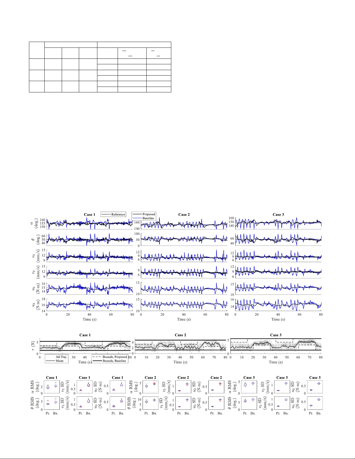
1   Performance Analysis for Almost Periodic Piecewise Linear Systems with Application to Roll- to -Roll Manufacturing Control Christopher Mar tin, Edward K im, Enrique Vela squez, Wei L i, and Dongmei Chen , Member, IEEE Abstract — An almost p eriodic piecewise linear system (APPLS ) is a ty pe of piecewise linear system where the system cyclically switches between different modes, each with an uncertain but bounded dwell-time. Process regulation, especially disturbance rejection, is critical to the per formance of these advanced systems. However, a method to g uarantee disturbance rejection has not been developed. The objective of this stud y is to develop an   performance analysis m ethod for APPLS s, building on whi ch a n algorithm to s ynthesize practical   controllers is proposed. As an application, the d eveloped metho ds a re demonstrated with an advanced manufacturing s ystem − roll- to -roll (R2R) dry tra nsfer of two-dimensional materials and printed flexible electronics. Experimental results show that the p roposed method enables a l ess conservative and much be tter performing   contro ller compared with a baseline   controller that does not acco unt for the uncertain system switching structure. Index Terms — Switching control, o ptimal control, roll- to -roll manufacturing, transfer of advanced materials. I. INTRODUCTION any engineer ing systems can be modeled as a piecewise linear system, where t he system b ehavior is d efined by different linear eq uations in different conditions. When the system behavior repeats periodically over time, these systems are called period ic p iecewise linear systems (PPLSs) [1 ] – [4] . In many cases, th e dwell times, wh ich ar e the amounts of time that the system spend s in each system mo de, of PPLSs ar e uncertain b ut bounded [5], [6]. Such systems are called alm ost perio dic p iecewise linear sy stems (APPLSs), as the dwell-time uncertainty introduces slight aperiodicity [5], [7] . Fig u re 1 illustrates the switching stru ctures of a PPLS an d an APPLS, both with  number of modes. In the PPLS case, th e switching time between system m odes is deter ministic. For APPLSs, switching occurs within bounded time intervals, represented by the segments labeled     for switching from mode  to mode    , where  = 1, 2, 3, …, and  . Note that while there is bounded uncertainty in the switching times and thus th e dwell -time of each system mode, th e switching sequence in an APPLS is known. This work is b ased upon work supported primarily by the National Science Foundation under Coo perative Agreeme nt No. EEC-1160494 and CMMI- 2041470. Any opini ons, findings and conclusi ons or recomme ndations expressed in this mat erial are those of the author(s) and do not necessarily reflect the views of the National Science F oundation. (Corresponding author: Christopher Mar tin) Fig. 1. The PPLS v s. APPLS switch ing structure. There are S system modes. Each mode has a distinct linear dynamic model. An example of an APPLS is the newly developed roll- to -roll (R2R) manu facturing process for dry transfer o f two - dimensional (2D) materials and printed electronics [8] – [10] . Fig ure 2 shows a schematic of the process [10] – [12]. The functional material is first laminated between the donor and t he receiver substrates. The laminate is then unwound, passed through a set of guidin g ro llers, and peeled a part so that the functional material d elaminates from the d onor substrate while adhering to the receiver substrate. During the peeling p rocess, the functional materials to be transferr ed often exhibit a pattern. For example, in [13] an array o f MoS 2 strips were p eeled from silicon, and in [10], [12] a series of graphene samples were peeled from a copper growth substrate. The abrupt transitions between different sections in these patterns can be modeled with different linear dynamics using a switched system structure. Since the p eeling pattern is kn ow n in advance, the system follows a fix ed switching seq uence. However, in R2R systems, position er ror (also kn own as register error) is a common issue [14], m aking the switching times, and equivalently the dwell-tim es, uncertain. For tunately, there will be tolerance limits on reg ister erro rs in in dustrial R2 R applications, i.e., th e dwell -time uncertainty will be bounded [6], [15] . Fig. 2. The R2R dry transfer process Christopher Martin, Edward Kim, Enrique Velasquez, W ei Li, and Dongmei Chen are with The Wa lker De partmen t of M echanical Engineering, Th e University of Texas at Austin, Austin, TX, USA, (cbmar tin129@utexas. edu, edwardkim877 5@utexas.edu, enrique.velasq uez@utexas.edu, weiwli@austin. utexas.edu, dm chen@me. utexas.edu) 2||3 1 1||2 2 S||1 1 S T ime (s) 3 1 2 1 S PPLS: APPLS: Active Mode Unwinding Roller Rewinding Rollers T ension Rollers Receiver Substrate T ransferred Material Laminated Donor and Receiver Substrates Guiding Rollers Donor Substrate Peeling Front M 2 Previous research on APPLSs has been fo cused on stability and stabilization m ethods bas ed on linear matr ix i nequality (LMI) techniques [ 5] – [7], [1 6], [17] . Due to high -precision requirements fo r advanced APPLS systems, distur bance rejection becomes a cr itical con trol ob jective to maintain the system performan ce [ 15], [18]. To desig n such a controller, it is first necessary to analy ze the   performance, wh ich represents the worst-case disturbance rejection capability of the closed-loo p system [19] – [ 21] . Ho wever, no   performance analyses for APPLSs h ave been found in the literature. The n eed for a dedicated   analysis m ethod for APPLSs arises fro m th eir unique switching structu re. Existing   analysis method s for switched p eriodic systems d o not acco unt for dwell-time unce rtainty [16], [22]. The method developed in this study represents the first rigo rous   perfo rmance an alysis framework for cyclically switched linear systems that ac counts for bounded dwell -time uncertainty. In addition to the dwell- time uncertainty , the an alysis is also extend ed to h andle norm - bounded modeling uncertainties [23], [24], making it generalizable to uncertain APPLSs [6] where each system mode is allowed to have additive modeling unce rtainty. Furthermore, a con troller sy nthesis meth od is d eveloped to optimize the   performance of uncertain APPLSs. The d eveloped method is experimen tally validated on a n R2R dry transfer testbed for 2D materials. Notation: Th e Eu clidean n orm for vectors and the corresponding induced norm fo r matr ices are denoted by    . Scalars are r epresented using regu lar (n on- bold) fo nt (e.g.,  ,  ,  ), while v ectors are written in bo ld lowercase fo nt (e.g.,  ,  ), and matrices are expr essed in bold uppercase font (e.g.,  ,  ). The identity matr ix is denoted by  . II. P ROBLEM F OR MULATION A. The unce rtain APPLS modeling structure The uncertain APPLS under c onsideration is an APPLS with additive mo delling uncertainty in each mode. The almost periodic switching structure of such systems is cyclic with bounded dwell- time uncertainties. Explicitly, when                  , an u ncertain APPLS can be represented as  󰇗 󰇛 󰇜  󰇛       󰇛  󰇜   󰇜 󰇛 󰇜    󰇛 󰇜     󰇛 󰇜 󰇛 󰇜     󰇛󰇜    󰇛 󰇜 󰇛  󰇜 where 󰇛 󰇜    ,  󰇛󰇜     , 󰇛  󰇜     , and 󰇛 󰇜     , are the state, control input, disturbance input, and system output, respectively.      and      are the uncertainty weights in mo de  , an d  󰇛  󰇜    is uncertain and time-varying such that   󰇛  󰇜   . Thus,   and   ,  = 1, 2, …, an d  , parameter ize the mode -dependen t a dditive modeling u ncertainty. Additionally,    is the length o f a perio d,        is the switchin g time from mode  to mo de    in the  th period, and        is the switch ing time from mode  to mode 1 i n the  th period. These period -dependen t switching times are unknown but bounded, so that    󰇣     󰇢 . Withou t loss o f generality, let each switching pattern begin with the time segment where mode 1 must be activ e. Then,                                    . Thu s,   and   ,  = 1, 2, …, and  , parameter ize the dwell-time uncertain ty. Define         an d           as the durations of the time segments where m ode  must be ac tive and wher e t he switch fr om m ode  to    occu rs, respec tively. For a cyclically switched system w ithout dwell-time uncertainty (a PPLS),   is the d well-time in m ode  and       . This uncertain APPLS modeling s tructure is illustrated in Fig. 3 , along with the APPLS an d PPLS mod eling structur es for comparison purposes. The shaded re gion is where the uncertain linear dynamics can exist over time, while the solid line is an example trajec tory. B. Switching con trol structure To match the alm ost periodic s witching structure, the control structure considered in t his study is chosen to be switched, full- state feedback [6] as belo w, 󰇛 󰇜   󰇱   󰇛 󰇜   󰇣               󰇢     󰇛󰇜    󰇣              󰇢 󰇛  󰇜 where the fee dback gains,   ,     ,  = 1, 2 , …, and  , are pre- calculated offline. The b lock d iagram of the uncertain APPLS modeling stru cture in Eq. (  ) an d switched controller structure in Eq. (  ) is sum marized in Fig . 4 . The co ntrol objective here is to m itigate the impact o f  on  . To achieve this goal, the next section in troduces a novel   performance a nalysis m ethod for uncertain APPLSs. Th is result is then used to develop a no vel   controller with the s tructure given in Eq. (  ). III. C ONTROL D ESI GN A. Novel   performance a nalysis for uncertain APPLS s Th e o re m 1 es tab li she s t ha t th e un c e rt a i n APP LS de s c ri b e d in Eq . (  ), wh en co n tr olle d usi ng the sw it chi ng str u ct u r e defi ned in Eq . (  ) , a c hi e v es a gu a ra nte e d we i g ht e d   pe r fo r ma n c e, as de f i n ed in De f i ni ti on 1 bel o w , pro v i d ed it s at isf i e s th e s p ec i fi ed set of m at rix i ne qu al iti e s De fini tio n 1: Th e un ce r ta i n AP PL S gi v e n in Eq. (  ) is sa i d to ha v e a w ei g ht ed   p er f o rm a n c e  i f , fo r    ,    , a nd    , i t is ex p on e n ti al ly st abl e w he n    , a nd th e fo ll owi n g ho l ds fo r ze ro i nit ia l c o nd i ti ons a nd a ny n on - z er o  w it h fi n it e e ne r gy :         󰇛  󰇜  󰇛  󰇜          󰇛  󰇜  󰇛  󰇜    󰇛  󰇜 Th e o re m 1 : Let the r e be     ,      ,       ,     ,       ,   ,    ,     , a nd g i ve n co ns t a nt s   ,     ,     , a n d      s uc h tha t , for  = 1 , 2, … , a nd  , 󰇯                           󰇰   󰇛   󰇜 󰇯                                 󰇰   󰇛   󰇜 3 󰇯                                    󰇰   󰇛   󰇜         󰇛   󰇜         󰇛   󰇜           󰇛   󰇜                󰇛  󰇜 ar e sa t is f i e d, wh e re     󰇛          󰇜                      ,                                           ,                                                    ,                ,            , a nd  󰇛  󰇜      . T he n, fo r th e unc e rt a i n AP P LS in Eq . (  ) wi t h ze r o i ni t i al co nd i t i o ns , co n t r ol le d us i n g the s wi t ch i n g s t r uc t u re i n Eq . (  ) , wi th c on t r o l ga i ns         an d             , th e we i gh t e d   pe rf o r ma nce giv en in De fin i ti o n 1 ca n be gua rant eed , whe r e     ,         󰇧 󰇡         󰇢    󰇨 ,     󰇝   ,   ,   , … ,   󰇞 , an d     󰇝   ,   ,   , …,   󰇞 . No t e tha t for Eq. (  ) to ho l d ,     . Pr o o f: S e e Ap p e nd i x. In the pro o f, th e fol low i ng mode - de p e nd e n t L ya pun ov f u nc ti o n ( M DL F ) i s u s ed [ 6] , [ 7] .  󰇛  󰇜   󰇱  󰇛  󰇜     󰇛  󰇜    󰇣               󰇢  󰇛  󰇜       󰇛  󰇜    󰇣               󰇢 󰇛  󰇜 wh e r e         a nd             . In Eqs . (  ) an d (  ) ,       a n d           . Re mar k 1: T h e   pe rfo r ma nce b o un d i n D e fi n it i o n 1 is we igh te d by a de c a yi n g e xp o ne n t ia l t o fac i l it at e th e us e of the di s c on t i nu o us MDL F in Eq . (  ). Thi s prac tic e is c om m on in t he li ter at ure f or sw i tc hed sy s te ms [ 1 6] , [2 5 ], as the se MDL F di s c on t i nu i ti es all ow th e   per f or m a n ce an al y si s met h od to be ap p l ie d t o a b r o ad e r c l as s o f s yst em s . Re mar k 2: T heo r e m 1 c an b e r e ad i l y e xt ende d t o ot her M D LF ma t ri x st r uc t u re s , su c h as con t i n uo us t i me- v a ry i ng [7] , or di s c on t i nu o us t im e - va ryi ng [ 16 ]. Re mar k 3 : Th e LM I s in T h eo re m 1 a li gn wi th the sw i t ch i ng s t ru ct ure of APP LS s . Eq ua t i on (  .A ) bo u nd s the sy st e m out put du r i ng the ti me s e g me n ts whe n mo de  mu s t b e a ct ive , an d Eqs . (  . B ) a nd (  .C ) b ou n d the sys t e m o u t pu t duri ng the unc er t a i n t i me s eg me nts w h e n the swi t c h fr om mod e  t o  + 1 m us t occ ur . Ad d it ion al ly, E q. (  ) bou nd s the gro wt h o f t he s y st em whe n Fig. 3. The PPLS, APPLS, and u ncertain APPLS modelin g structures. Fig. 4 . Block diagram of uncertain APPLS mo deling and contro l structure.                                                                    …     …                 0   …   … T ime                                … System Dynamics     …                 0   …   … Uncertain APPLS: APPLS:                         …     …                    0   …   … PPLS: Increasing Generality                                                                                                   4 s wi t ch i n g betw e e n t h es e t ime s e gm e n ts . B. Weighted   controller synthesis Ut ili z i ng T he orem 1, a pra ct ica l   con t ro l l er sy nt h es is al gor it hm f or th e u n ce rtai n APP L S gi ve n in E q. (  ) w it h the co n t r ol s t ru c t ur e in Eq . (  ) is pre s en t e d be l ow i n Al gori thm 1 . The al gor it hm ha s tw o ph a s es ; th e fir s t ite r a te s un t il a d es i re d st abi li t y ma r g i n is ac hi e v ed , an d t h e se c o nd ite rat es to op ti miz e t h e we igh te d   pe r f or ma nce . In t hi s wa y st a b il i t y c a n be g ua ra nte e d, wh i l e dis tur b a nc e r e je ct ion can b e max i mi z e d. F o r t h e st ab il i t y ph a s e, t he f ol l ow i n g st a b il i zi ng LM I res ult wi ll b e use d [6] . I f t he r e is     ,       ,       ,     ,       ,   ,    , a n d give n c o ns t an t s   ,    ,     , a n d      s uc h th a t ,   󰇛          󰇜                       󰇛   󰇜 󰇯                                            󰇰 󰇛   󰇜 󰇯                                                󰇰 󰇛   󰇜 an d Eq s . (  ) a n d (  ) h ol d, t h e n, as s um i n g    , i t c an be r e ad i ly pr o ve n tha t the unce r t ai n APPL S in Eq . (  ) i s   -e x p on e n ti a ll y s ta b il i z ed by th e con t r ol l a w in Eq . (  ) wi t h         , an d             . Mor e det ail s ca n be fou nd i n [6] . Ad d it ion al ly, t h e fo l l ow i ng p r a ct i c al con st rai n t o n t he no rm o f t he co n t r ol l e r gai n is in t ro d u ce d. If    󰇣        󰇤   󰇛  󰇜 th e n      , wh e r e     [ 26 ] . In Alg or i t hm 1, Eq. (  ) wi ll be a p pl i e d t o t h e pa i rs   ,   a nd    ,     t o e ns u r e t hat th e n or ms of   a n d    a r e bo u n de d. Algorithm 1:   Contr ol Design (HCD ) Step 0: Choose    ,     ,      ,      ,    , and     Phase 1: Guaran tee Conver gence Step 1.1: Set     and    . If Eqs. (  .A) and (  ) hold for some     and   when     :      . Else :       . If Eqs. (  .B), (  .C), and (  ) hold for some      and    when      :       . Else :        . Step 1.2: W it h    ,     ; find    ,     ,    ,     , such that Eqs. (  ), (  ), and (  ), hold. Step 1.3: W it h    ,     ,    ,     ; find         that minimize                      subject to Eqs. (  ) and (  ). Step 1.4: If      or          : go to Phas e 2. Else:   , return to Step 1.2. Phase 2: Optimi ze W ei ghted   Performance Step 2.1:       ,         from end of Phase 1.     . Step 2.2: W it h    ,     ; minim ize   over    ,     ,    ,     , such that Eqs. (  ) , (  ) and (  ) hold. Step 2.3: W it h   ,    ,     ,    ,     ; find    ,     that minimize   subject to Eqs. (  ) and (  ). Step 2.4: If          : ST OP . Else:   , return to Step 2.2 . Stability Check: If     , where   is from the en d of Phase 2, then the feedback gai ns         and            achieve a weighted   performance  for the system d efined by Eqs. (  ) and (  ). Also, for    , the same syst em is   -exponentially s table. Re mar k 4: T he nov el   c on t ro l f r a me w or k pr es ent e d in Th e o re m 1 an d A l g or i t hm 1 i s de s i gn e d fo r u n ce r t ai n AP P LS s , and it c an al s o re adi l y b e ap p li ed t o A P P LS s , si n c e u n ce r ta in A PP L S s ar e a ge ne r al izat ion o f AP PLSs . Re mar k 5 : Al go ri thm 1 ca n b e us e d t o a ch i ev e o pt i ma l pe r f or m a nc e wit h ou t s i gn i fi c an t onl i ne com p u t at i o n sin c e th e un c e rt a i n A PP LS st ruc t ur e ass ume s kn o w n mode - de pend e nt dy n am ics a n d unp re d ic tab l e dis t u rb a nc e i n pu ts , maki ng a d a pti ve   c on t r ol a p pr o ac h es [27 ] , [28 ] u n ne c es s a r y an d me tho ds t hat le arn di st urb a nc e cha rac t er i st ics on l i ne [2 9 ] ina p pl i ca ble . Th us , th e   con t r ol l e r sy n t h es i s ca n a c hi ev e op ti m al pe rfo rm a nc e w hi l e ma i n ta i ni ng a p ra cti ca l st r u ct u re t ha t i s co m pa t i bl e w i t h in d u st ri al ap p l ic a t io ns t ha t ha ve li mi t ed on l i n e c om p u ta ti ona l r e s ou r ce s . IV. C ASE S TUDY : R2R D RY T RANSFER The un certain APPLS analysis and control framework developed in Section I II is applied to the R2R dry transfer of patterned materials, addressing the system switching dynamics and mode -dependent uncertainties. Exp erimental results demonstrate the effec tiveness of the novel   con troller i n improving peeling angle control and overall system performance. A. The R2R dry transfer pa tterned p eeling dynamic model This subsection summ arizes the R2 R dry transfer p atterned peeling dynam ic model [6], [9], [30] . Fig. 5 depicts the peeling front o f the R2 R dry transfer system, and Tab le I lists the physical p arameters. In the figure, differ ent web colors represent different web material sections. Each material section is rep resented as a different dynamic mode in the system model, because certain material parameters will ch ange depending o n which section o f the web is bei ng peeled. These pattern section- dependent v ariables are listed at the en d of the table. The we b ve lo ci ty deri va ti ve s of t he R2 R dr y t ra nsfe r syst em ar e giv en a s f oll ows,  󰇗  󰇛  󰇜          󰇛  󰇜        󰇛  󰇜        󰇛  󰇜      󰇛  󰇜 The w e b te nsi on d yn a mic s c an b e de t er mi ne d as a f unc ti o n of t he uns t ret c he d l e ng th de riva ti ve s a s  󰇗       󰇛  󰇜    󰇗      󰇛  󰇜    󰇗      󰇛  󰇜    󰇗      󰇛  󰇜 whe re Fig. 5. R2R dry transfer of a patterned material. W eb 1 W eb 3 W eb 2                  Section Numbers Roller 3 Roller 2 Roller 1 v p               5 TABLE I R2R PEELING PARAM ETERS Variable Description (U nits)   ,  = 1, 2, 3 Tension in web  (N)   ,  = 1, 2, 3 Velocity of web  (m/s)   ,  = 1, 2, 3 Unstretched le ngth web  (m)   Peeling angles (ra dians)   ,  = 1, 2, 3 Strain in web  (m/m)   ,  = 2, 3 Motor torque i nputs (N- m)   Peeling front velocity (m/s)         Bending curvatur e of web  (1/m)         Elastic modulus of web  (N/m 2 )   ,  = 1, 2, 3 Radius of roller  (m)   ,  = 1, 2, 3 Moment of inerti a roller  (kg-m 2 )   ,  = 1, 2, 3 Friction coeffic ient of roller  (m/s) Pattern Section-D ependent Para meters          Moment of Inert ia of web  section  (m 4 )   Adhesion Ener gy of sectio n  (J/m 2 )   Width of the con tact surface of section  (m)   󰇗 󰇛  󰇜    󰇛  󰇜    󰇛  󰇜     󰇛  󰇜 󰇛    󰇜   󰇗 󰇛  󰇜    󰇛  󰇜   󰇛  󰇜    󰇛  󰇜   󰇛  󰇜      󰇛    󰇜 The un st r et ch ed le n gth s ar e p ro po rt io na l t o t he am ou nt of m as s i n a web and the se nsi ti vi t ie s     can be fou nd n ume ri ca l ly [15 ], [18 ] . Fi nal l y, ass uming con st a nt pe el in g and negl ec ti n g hig he r-o r de r ter ms , t h e e ner g y b al a nce at t he pee l in g f ro nt ca n b e su mma ri z ed as           󰇛  󰇜 whe re                                   󰇛  󰇜 B. Representing R2 R peeling as an uncertain A PPLS Nex t, the pe eli n g ang le s, whic h are ill us tr at ed in Fi g. 5, ca n be fo und as a f un ct i on o f the thr ee web t en si ons.                    󰇛    󰇜                   󰇛    󰇜 The peel in g angl es have b ee n sho w n t o have a di r ect impa ct on the tran s fer qual it y of the R2 R dry tra ns f er proc es s [10] , [12] . In add it io n, cont rolli ng thes e an gl es is cha ll e ngi n g, as ev en smal l cha ng es in web ben di ng ene rg y and adhe si on ca n lea d to si gni fi ca nt e rr or s. Thus , t he pri mar y c ont rol goa l in this s tu dy is to reg ul at e t he peel in g an gl es a t a s et p oi nt [ 8] – [1 0] , [1 3] , [3 1] . Us ing E qs . (  )-(  ), the nonl in e ar s ta te dynam ic s c an be com pa ct ly r e pr es ent ed as fol l o ws ,  󰇗 󰇛󰇜    󰇛 󰇛 󰇜 󰇛󰇜  󰇛 󰇜 󰇜 󰇛  󰇜 whe re   󰇟          󰇠  are t he sys t em s ta t es ,        ar e the dis tu r ban ce inp ut s, and   󰇟      󰇠  are the co nt rol in pu ts . Whe n mo de  is act iv e, the non li ne a r sys te m dyna mi cs in Eq . (  ) can be re la xe d i nto th e fol l ow in g li ne a r dif fe r ent i al incl usi on (LD I) [ 6] , [ 15 ], [ 18 ]:  󰇗 󰇛󰇜   󰇛   󰇜 󰇛 󰇜    󰇛 󰇜      󰇛 󰇜 󰇛  󰇜 whe re                 and       ; an d   ,   , and   are ref er en ce sig nal s . Ad di ti o nal l y,        is con st a nt,         is treat ed as cons ta nt s i nce    does not va ry mu ch with res pe ct to  ,  󰇛  󰇜 i s t he co nv ex hu l l oper at or , a nd   i s th e LDI se t d ef i ned a s foll ows ,                󰇣     󰇤    󰇣     󰇤 󰇛  󰇜 whe re      an d     ar e the low er and uppe r boun ds of   an d  , res p ect i vel y. Note that , sinc e         ,   , and   ar e mo de - dep en de nt , t he bo un ds o n  are al s o m ode - dep e nd en t, w hi le t h e bou nd s on   are not . This LD I ca n be re pr es e nte d as a li n ea r sys t em wi th nor m-bou nd ed unc ertai nty [ 1 5].  󰇛  󰇜 󰇗  󰇛       󰇛  󰇜   󰇜  󰇛  󰇜   󰇛 󰇜     󰇛 󰇜 󰇛  󰇜 Th us, each ma t eri al mo de c an b e nat ur al ly model e d as a li near sys t em wi th ad dit i ve , no rm -b ou nde d un ce rt ai nt y . To dete rm i ne t he s wi tc hi ng sig nal , it i s as s um ed t ha t the pee l in g fol l ows a p re di ct able p at te r n wi th  p ee li ng modes , s uc h th at mod e    is pe el ed im me di at el y a ft er m ode  , as i n F ig. 5. In add it io n, i t is ass um ed t ha t t his pa tt er n is c yc li c, s o t hat mo de 1 i s pee le d im me dia tely afte r mode  . Let   be cons ta nt and defi ne   and   as the close st a nd far th es t dis ta nc e, re la ti ve to the sta rt of the patt e rn , that mode  can s witch t o mod e    , r es pe ct iv el y . Unde r t hes e ass um pti ons, the R2R patt er ned pee li ng sys te m can be re pr es e nte d as a n un ce rt ai n APPL S, w her e          󰇛    󰇜                     󰇛    󰇜 and th e lin ea r mod es wit h mod el i ng unc ert aint y are give n in Eq. (  ). Fig ure 6 s um ma ri ze s t he pr oce s s o f re pr es en t in g R2 R pa tt erne d pee li ng as an un ce rt a in APP LS . Fig ure 6( a) sh ows t he sys t em wi t h two s ecti on s, or mod es . Fig u re 6(b) plot s t he bo un ds on the unc er t ain vari ab le s,  and   , ove r time . Acco r di ng to Eqs . (  ) and (  ) , t hes e bo un ds ca n be used to rep re se nt eac h dyn am ic mod e as a li near s ystem w i th a dd it iv e model l in g un ce rt ai nt y . In Fig. 6. Representing R2R dry transfer of patterned mater ials as an uncertain APPLS.                                                                                 0              System Dynamic s T ime T ime Bounded Uncertain V ariables (b) (a) (c) 6 add it io n, the swi tc hing ti mes on thes e bound s, der iv ed usin g Eq. (  ), als o d efi ne the un ce rt ai n s wi tc hi ng time s of t he sys t em . Fi nal l y, F ig . 6(c ) ill ustra t es the uncer t ain AP P LS mode li ng st ruc t ur e fo r t his pa tt er n ed p eel i ng s ys te m. C. Baseline con troller design and controller tuning The pr op os e d   cont roll er fo r un cer ta i n APPL Ss , de vel oped in Se ct i on II I, is app l ied to re g ula te R2R patt er ne d pee l in g on an exp er i me nta l t es t be d, repr es enti ng t he fi rs t e xp er i me nt al val i dat i on of a swi tc hing c on tr ol met ho d for R2R pe el in g. In thi s st ud y, t he cont rol obj ec ti ve is to reg ul at e the syst e m stat es d efi ned in Eq. (  ) ar ou nd an opti mal set po int , prior i ti zi ng the crit ic a l pee li ng a ng les t o e ns ur e t heir p re ci se co nt r ol. The pe rf or ma nc e of the p ro po se d contr olle r i s com pa re d a ga in st a ba s el in e time- inv ar ia nt , no n-s w it ch in g   -opt i mal ful l- st at e -f eed ba c k con tr ol le r. Th is c ont roll er is t he onl y   con t rol l er t hat has b ee n app li ed to R2R pee l in g in the lit era t ur e [15 ]. Th e bl ock dia gr a m of th is bas el ine c ontro l le r is s hown i n Fi g. 7 . Thi s ba s eli ne con tr ol le r is s ynt h es iz ed a n d im pl em en te d wi t ho ut uti li zi ng th e a-p ri o ri know le d ge of the pe elin g p att ern, inst ead rel yi n g o n a lin ear ti me inv a ria nt (L TI ) mod el of th e s yst e m w it h add it iv e nor m- b oun de d un ce rt ai nt y. Th e nom i nal lin ea r dyna m ic s of t he bas el in e sy st e m ar e de fi ned as t he avera ge of th e sy st e m mat ri ce s acro ss all m od es , 󰇛      󰇜              . Addi t io na ll y, the a dd it iv e mo de ll in g un ce rt ai nt y, par ame t eri zed by  and  , is co ns tr uct e d unde r the ass um pt io n that  ca n vary bet we en it s ma xi mu m a nd min im um bou nds ac ros s al l peeli ng mod es . As a res ul t , t he ba se li ne contr ol le r is ov erl y c on se rv a ti ve , whi le t he pro pos e d cont r oll er prop er l y inco rp or at es t he a-pr i ori kno wl ed ge of t he p eel i ng p at te r n. Fi g. 7. B l ock d ia g ra m f o r t he b as el ine co nt rol ler. To en su re fa i rn es s of co mp a ris on, t he  par ame t er fr om E q. (  ) was adj us te d ind e pe nd ent l y so th at , for bot h co nt rol l er s,      , whe re  is give n in Th eo rem 1. Thus , bot h cont r oll ers gua ra nt ee the s am e   pe rf or ma nc e. A dd it io na ll y, t he   and   mat ri c es , whi c h w ei g h t he cost of s ta te e r ro r and c ont r ol e ff or t, as desc ri b ed in Eq. (  ), a re ide nt ic al for b ot h cont rol l er s. S pec i fic al ly,    󰇣    󰇤 and         whe re   and   are d ia g on al mat rices tun ed usi ng Br yso n’ s rule [32] , s uc h tha t        and        . Addi t io nal wei gh t was put on the cel ls in   t ha t cor re sp o nd to t he pe elin g a n gl e erro rs . Als o,     ,         , and      for both co nt rol l er s. Sinc e t he con t ro l goa l i s t o r ej ec t t he di st ur ba nces ca us ed by  and   ,     so tha t  wil l be a s s mal l a s po ss ib l e wh il e st il l e ns u rin g st a bi li t y. D. Experimental setu p The experimental setup of the R2R testbed is shown in Fig. 8 . The roller velocities and web tension s are measured using encoders on the two rewinding rolls and loadcells on each of the three web sections, as illustrated in Fig. 8(a). The control hardware uses a National Instrument CompactRIO to collect these measuremen ts [15] . The tension m easurements are used to calculate  ,  , and  online according to Eqs. (  )-(  ). The controller produces voltag e outpu ts to actuate the brushless motors that d rive the two rewinding rollers. Fig ure 8(b) shows the peeling p attern. T wo different p eeling modes were created using two types of scotch tape peeled from a po lyethylene terephthalate (PET) web . The two types o f tap e have significantly differ ent adhesion properties. Fig ure 8( b) also dep icts the relatio nship between switching par ameters (   ,   ,   , and     ) and the material mode switch lo cations. For each p eriod of each experimental run, th e switch from mode 1 to mode 2 is randomly cho sen to be between   and   , simulating the dwell-time uncertainty characteristic of advanced R2R processes. An analogo us approach is used to choose the switch locations from mode 2 to mode 1. The physical par ameters of the setup are given in T able II [15]. Experimen ts were conducted u nder three different operating cases. The angle setpoints, unwinding velocities, and peeling patterns of each case are g iven in Table III. Six experiments were run for each case. The condition s of this experimen t are relevant to any R2R pee ling process, as th e key dyn amic factors — such as fluctuating and unpredictable adhesion energy, bending energy, and peeling front velocity — clo sely resemble those in peeling advanced 2D materials. For exampl e, Eqs. (  ) and (  ), wh ich were u sed to design the controllers, were origin ally developed to model th e R2R dry tr ansfer of graphene [9]. Thus, the result can be scaled as necessary for industrial R2R peeling processes. Fig. 8. R2R peeling experim ental testbed. (a) The R2R machine; (b) Th e peeling pattern . TABLE II P ARAMETERS OF T HE EXPERIMENT AL SYSTEM         (GPa)         (m)            (mm 2 )      (kg-m 2 )      (N -m-s-rad -1 ) 2.0 0.0381 15.5, 12.9, 12.9 0.65, 0.75 9.2, 11.4                                                                        Roller 3, Encoder Roller 2, Encoder Roller 1 Load Cell Load Cell Load Cell Peeling Front (a) (b) T ape 1 T ape 2 7 TABLE I II T HE THREE EXP ERIMENTAL CASES Case Setpoint Peeling Pattern Pr operties  (deg.)  (deg.)   (cm/s) Section   ,   (cm)   ,   (s) 1 50 155 1.1 Tape 1 16.5, 22.0 15, 20 Tape 2 38.5, 44.0 35, 40 2 56 152 .73 Tape 1 11.0, 14.7 15, 20 Tape 2 25.7, 29.3 35, 40 3 56 147 .88 Tape 1 13.2, 17.6 15, 20 Tape 2 30.8, 35.2 35, 40 E. Results and discu ssion Fig ure 9 shows one representative example trajector y fo r each of the three experimental cases. Fig ure 10 gives the measured  signals for all the experimental runs. In the figure, the black dashed lines g ive the mod e-d ependent upper and lower bo unds of  th at were used to generate the u ncertain APPLS system model for the p roposed contr oller. The heavy solid black lin es are the uniform upper and lower bound s o f  that were used to generate the conserv ative uncertain system model fo r the baseline controller. Fig ure 11 giv es box plots of the RMS er rors of the two peeling angles and the stand ard deviations of th e velocity and co ntrol signals for each ca se. The example trajectory in Fig. 9 shows that the baselin e controller induces far m ore undesired variations th an th e proposed controller. Furthermo re, Fig. 11 shows that the proposed con troller achieves less mean RMS angle er ror than the baseline co ntroller, and the baseline controller in duces significantly more velocity and control variation. Specifically, over the three cases, the mean RMS  er ror is d ecreased by an average of 17.5% relative to the baseline, while the mean RMS  error is dec reased b y an ave rage of 1 9.6%. This dif ference would have a significant impact o n peeling performance o f advanced mater ials [10], [13]. In addition, over the three cases, the mean   ,   ,   , and   stan dard d eviations are decreased by an av erage o f 69.9 %, 67.5 %, 63 .5%, an d 62.7%, respectively, relative to the b aseline. Over time, excessive variations in web velocity and motor torque would result in significant wear to p rocess components and actu ator s. Thus, the proposed controller ach ieves significantly better perf ormance than the b aseline controller. The baseline co ntroller results in wor se performance because it is highly c onservative. Specifically, b ecause the controller synthesis pro cedure does not accoun t for the peeling pattern, the controller gain must be made too high to guarantee th e same   performance the proposed controller. This unnecessarily high-g ain feedback excites un modeled dynam ics, resulting in severe oscillations. Additionally, as shown in Section IV.B, the dwell-time and mo deling uncertainty included in the un certain APPLS structure is necessary to ac count for the nonlinearities and parameter varian ce inh erent in th e system. The resu lts show that the propo sed un certain APPLS   analysis and control design p rocedure finds the op timal tradeoff by considering the Fig 9. Example experimen tal state and control tr ajectories Fig. 10 . Experimental τ variation Fig. 11 . Angle erro rs, velocity variation, and contr ol variation. “Pr.” stands f or the proposed controller an d “Ba.” stands for the baseline contr oller. 8 correct amount of uncer tainty to ensure that the necessary performance is achieved, without being too conservative such that a high control gain would harm system performance. V. C ONCLUSI ON This study presen ts a novel switched system analysis and control framework f or uncertain APPLSs w ith diver se applications. The APPLS structu re extends the standard PPLS by incorporating d well-time uncertainty, while the uncertain APPLS i s a fu rther generalization that accounts for m odeling uncertainty. To fac ilitate controller synthesis, an   performance resu lt is established for APPLSs an d uncertain APPLSs. The theo retical treatment utilizes the sy stem switching structure an d a discontinu ous, time -varying, MDLF. The novel   performance result is leveraged to develop an   controller synthesis alg orithm for unce rtain APPLSs. The resulting control policy can achieve optimal perform ance without costly online computation. This novel   controller is applied to R2R d ry tran sfer of p atterned 2D materials. Experimen ts wer e conducted and the results demonstrate that the proposed method enables a less conservative and, therefore, better-per forming con troller. The proposed co ntroller reduced the average peeling angle error by 19% and the average cont rol input and motor speed variation by 69% and 63%, respectively. This improv ement in performance will sign ificantly increase the transfer quality and drastically red uce component wea r. Future work could relax th e curr ent modeling assum ptions for each mode, th us extending the almost p eriodic p iecewise switching framework to a broader class of systems. Fo r example, the assump tion of known nominal dynamics could be lifted, enabling the use o f adaptive or mod el-free meth ods th at learn the d ynamics or optimal contr ol policy for each mode online. Additionally, alternative un certainty structures — such as structu red, multiplicative, or time -v arying unce rtainty — could b e introduced to m atch a given application. L ikewise, with advancements in m achine lear ning, data -driven techniques could be integrated to enhance con trol of processes with an APPLS structure, such as R2R dry transfer. Hybridizing such a data-driv en appro ach with a -priori knowledge of system dynamics could furth er imp rove accu racy while maintaining understand ing of the process physics. Th e work presented in this study provides critical foundation for these potential extensions. A PPENDIX Proof of Theorem 1 : First, Eqs. (  )-(  ) guarantee that the uncertain APPLS in Eq. (  ), controlled using the control structure in Eq. (  ), is   -exponentially stable wh en    [6], [7]. T his stability result ca n be pr oven using the MDLF in Eq. (  ) [6], [7] . Next, Eq. (  ) can be rearranged into the following set of LMIs. 󰇯                󰇛     󰇜      󰇰   󰇛    󰇜                                     󰇛    󰇜                                      󰇛    󰇜 where       󰇛        󰇜        󰇛        󰇜  󰇛        󰇜         ,       󰇡            󰇢                                         ,       󰇡              󰇢                                              ,       ,         ,         ,              ,       ,         , and          . Using the  -procedure [33], Eq. (  ) implies that, for   󰇣               󰇢 ,      󰇗                     󰇛  󰇜 and for   󰇣               󰇢                  ,      󰇗                        󰇛  󰇜 Then, Eqs. (  ) and (  ) lead d irectly to the following bound s on the MDLF in Eq. (  ). For   󰇣                 󰇢 ,  󰇗 󰇛  󰇜     󰇛  󰇜  󰇛          󰇜 󰇛  󰇜 and for   󰇣               󰇢 ,  󰇗 󰇛  󰇜       󰇛  󰇜  󰇛          󰇜 󰇛  󰇜 Next, Eq. (  ) can be rearranged to yield the following relationships.         󰇛    󰇜         󰇛    󰇜            󰇛    󰇜 where       and          . Then, using Eqs. (  )- (  ), and the definition of  󰇛  󰇜 in Eq. (  ), the following bound on  󰇛  󰇜 for   󰇣               󰇢 can be established, relative to the initial condition  󰇛  󰇜 , using convo lution.  󰇛  󰇜      󰇛  󰇜    󰇩     󰇛  󰇜  󰇛   󰇜      󰇛   󰇜                 󰇛  󰇜  󰇛   󰇜      󰇛   󰇜              󰇛  󰇜                    󰇛  󰇜                      󰇛  󰇜                    󰇛  󰇜         󰇛  󰇜 where  󰇛  󰇜    󰇛  󰇜  󰇛  󰇜      󰇛  󰇜  󰇛  󰇜 , and th e   ,        ter ms are defin ed below. 9           󰇛    󰇜                                           󰇡       󰇢 󰇛    󰇜           󰇛      󰇜         󰇛    󰇜                󰇛    󰇜                                   󰇛    󰇜                         󰇡       󰇢 󰇛    󰇜           󰇛      󰇜         󰇛    󰇜            󰇡 󰇛    󰇜         󰇢         󰇛    󰇜                         󰇡        󰇢 󰇛    󰇜                  󰇡         󰇢                        󰇡        󰇢 󰇛    󰇜                                          󰇡       󰇢 󰇛    󰇜           󰇡         󰇢      󰇡       󰇢 󰇛    󰇜        󰇛    󰇜 󰇛    󰇜 In th is way , the MDL F in Eq. (  ) is b ounded by a stable linear system that is solved explicitly, creating a homogenous term and a par ticular term that depends on the difference between the weighted input a nd output norms,  󰇛  󰇜 . Next, to get an inequality that bounds the weig hted signal norm of  by the signal n orm of  , n ote that  󰇛  󰇜   , and multiply both sides of Eq. (  ) by   , where    󰇛    󰇜                                           . This gives the following relationship.   󰇩      󰇛  󰇜   󰇛   󰇜      󰇛   󰇜                  󰇛  󰇜   󰇛   󰇜      󰇛   󰇜         󰇩      󰇛  󰇜                       󰇛  󰇜                       󰇛  󰇜                      󰇛  󰇜               󰇛  󰇜 󰇛  󰇜   󰇱  󰇩      󰇛  󰇜   󰇛   󰇜      󰇛   󰇜                   󰇛  󰇜   󰇛   󰇜      󰇛   󰇜         󰇩      󰇛  󰇜                       󰇛  󰇜                      󰇛  󰇜                      󰇛  󰇜           where the   ,        and   ,        terms are defined below.                             󰇡       󰇢 󰇛    󰇜                              󰇛    󰇜           󰇛    󰇜                        󰇡       󰇢 󰇛    󰇜        󰇡 󰇛    󰇜        󰇢         󰇛    󰇜                        󰇡       󰇢 󰇛    󰇜      󰇡         󰇢                      󰇡       󰇢 󰇛    󰇜                                   󰇡       󰇢 󰇛    󰇜      󰇡         󰇢      󰇡       󰇢 󰇛    󰇜       󰇛    󰇜 󰇛    󰇜       󰇛    󰇜                      󰇛    󰇜 10       󰇛    󰇜                  󰇛    󰇜                              󰇛    󰇜                         󰇛    󰇜                             󰇛    󰇜                         󰇛    󰇜 To combine terms in Eq. (  ), starting with the definitions of   ,        and   ,        , the following ch ain of inequalities can b e proven.       󰇛    󰇜                         󰇛    󰇜                                    󰇤            󰇟          󰇠   󰇛            󰇜     󰇛      󰇜       󰇛  󰇜 By similar lo gic, it can be shown that   ,   ,   ,   , and      󰇛      󰇜       . Additionally ,                                           󰇛       󰇜󰇛      󰇜      󰇛      󰇜    󰇛  󰇜        󰇛    󰇜                                                󰇛    󰇜           󰇛    󰇜  󰇛      󰇜  󰇛    󰇜  󰇛    󰇜        󰇛    󰇜  󰇛      󰇜    󰇛  󰇜 By similar logic, it can b e shown that   ,   ,   ,   , and      󰇛    󰇜  󰇛      󰇜    . Finally, these bounds o n the exponential coefficien ts allow Eq. (  ) to be s implified as follows,   󰇛   󰇛     󰇜      󰇜   󰇛  󰇜  󰇛  󰇜      󰇛     󰇛     󰇜    󰇜  󰇛  󰇜      󰇛   󰇛   󰇜  󰇛     󰇜    󰇜   󰇛  󰇜  󰇛  󰇜    󰇛  󰇜 Then, integrating  from  to  an d dividing by       , the following r elationship follows.       󰇛  󰇜  󰇛  󰇜      󰇛  󰇜        󰇛  󰇜  󰇛  󰇜    󰇛  󰇜 where         󰇡 󰇛     󰇜    󰇢 , and  and  are defined in the th eorem statement. Equation (  ) is a weighted   -gain criterion for the system [16], [ 17]. Assumin g zero in itial conditions, Eq. (  ) is eq uivalent to the weighted   performance result in Eq. (  ) . □ R EFERENCES [1] J. Jiao et a l., “Dynamics of a periodic switched predator– prey system with impulsive harvesting a nd hiberna tion of prey p opulation,” J Franklin Inst , vol. 353, no. 15, p p. 3818 – 3834, Oct. 2016. [2] C . W. Wong et al., “Perio dic forced vibration of u nsymmetrica l piecewise- linear systems by incr emental harmo nic balance m ethod,” J Sound Vib , vol. 1 49, no. 1, p p. 91 – 105, Aug. 1991. [3] Ji an Sun et a l., “Average d modeling of PWM converter s operating i n discontinuous co nduction m ode,” IEEE Trans Power Electron , vol. 16, no. 4, pp. 482 – 492, Jul. 2001. [4] S. Teng et al., “A Least -Laxity-Firs t Sched uling Algorithm of Variable Time Slice for P eriodic Tas ks,” International Jour nal of Soft ware Science and Com putational I ntelligence , vol. 2, no. 2, pp. 86 – 10 4, Apr. 2010. [5] B . Wei et al., “Stability A nalysis of C ontinuous -Time Alm ost Periodic Piecewise Linear S ystems wit h Dwell Time Un certainties,” in Proceedings of the 43rd Chin ese Control C onference , 2024, pp. 1153 – 1159. [6] C . Martin et al., “Stabiliza tion of Almost Periodic Piecew ise Linear Systems with Norm- Bounded Un certainty for Roll- to -Roll D ry Transfer Manufacturing Pr ocesses,” i n 2024 America n Control Co nference (ACC) , 2024, pp. 1121 – 1126. [7] C . Fan et al., “Stability and S tabilizati on of Almost P eriodic Piecew ise Linear Systems W ith Dwell T ime Uncertai nty,” IEEE Trans Aut omat Contr , vol. 68, n o. 2, pp. 1130 – 113 7, Feb. 2023. [8] N. Hong et al., “The Line S peed Effect in Roll - to -Roll Dry Transfer of Chemical Vapor Deposition Gra phene,” Inter national Confere nce on Micro- and Nano- devices Enable d by R2R Manufacturi ng , 2021. [9] N. Hong et al., “A method to estimate adhe sion energy of as -grown graphene in a r oll- to - roll dry transfer pro cess,” Carbon N Y , vol. 201, pp. 712 – 718, Jan. 202 3. [10] N. Hong et al., “Roll‐ to‐Roll Dry Tr ansfer of L arge‐Scale Gr aphene,” Advanced Materi als , vol. 34, n o. 3, Jan. 2022. [11] S. R. Na et al., “Selec tive mecha nical transfer of graphene from seed copper foil usi ng rate effects ,” ACS Nano , vol. 9, no. 2, pp. 13 25 – 1335, Feb. 2015. [12] H. Xi n et al., “Roll - to -r oll mec hanical peeling f or dry transfer of chemical vapor deposition gr aphene,” J Micro N anomanuf , vol. 6, n o. 3, Sep. 2018. [13] J. Zhao e t al., “Patter ned Peeling 2D MoS2 off t he Substrate,” ACS Appl Mater Interfaces , v ol. 8, no. 2 6, pp. 16546 – 16550, J ul. 2016. [14] K. H. Choi et al., “W eb register control algorithm for roll - to -roll system based printed ele ctronics,” in 2010 IEEE Inter national Confer ence on Automation Sc ience and En gineering , 2010. [15] C. Mar tin et al., “Op timal Control of a Roll - to -Roll Dry Transfer Pr ocess With Bounded Dy namics Conv exification ,” J Dyn Syst Meas Control , vol. 147, no. 3, p. 031004, M ay 2025. [16] P. Li e t al., “Stabili ty, stabilization and L2 -gain analysis of periodic piecewise linear s ystems,” Autom atica , vol. 61, pp. 218 – 226, N ov. 2015. [17] Panshuo Li et al., “St ability and L2 -g ain analysis of periodic piecew ise linear systems,” in 2015 America n Control Co nference (ACC) , 2015, pp. 3509 – 3514. [18] C. Mar tin et al., “H∞ O ptimal Co ntrol for Main taining the R2R P eeling Front,” IFAC-Pa persOnLine , vol. 55, no. 37, pp. 663 – 668, 2022. [19] X. Xie et al., “Finite - tim e H∞ control of periodic pie cewise linear systems,” Int J Syst Sci , vol. 48, no. 11, pp. 2 333 – 2344, Aug. 2017. [20] P. Li e t al., “H∞ co ntrol of periodi c piecewise vi bration syst ems with actuator saturati on,” JVC/Journ al of Vibrati on and Contro l , vol. 23, no. 20, pp. 3377 – 3391, Dec. 2017 [21] X. Xie et al., “H∞ c ontrol problem of linear peri odic piecewis e time - delay systems, ” Int J Syst Sci , vol. 49, no. 5, pp. 997 – 1011, Apr. 2 018. 11 [22] P. Li e t al., “Stabili ty and L2 Syn thesis of a Class of Periodic Pi ecewise Time- Varying S ystems,” IEEE Tra ns Automat C ontr , vol. 64, no. 8, pp. 3378 – 3384, Aug. 2019. [23] X. Xie et al., “Robust ti me -weighted guaranteed cost control of uncertain periodic piecew ise linear s ystems,” Inf Sci (N Y) , vo l. 460 – 461, pp. 238 – 253, Sep. 2018. [24] C. Fan et al., “Peak - to - peak filter ing for peri odic piecewise linear polytopic systems ,” Int J Syst Sc i , vol. 49, n o. 9, pp. 1997 – 201 1, Jul. 2018. [25] Y. Liu et al., “Stabiliza tion and L2 - g ain performan ce of periodi c piecewise impulsi ve linear sys tems,” IEEE Access , v ol. 8, pp. 200 146 – 200156, 2020. [26] A. I . Zecevic and D. D. S iljak, “St abilization of n onlinear sys tems with moving equilibr ia,” IEEE Trans A utomat C ontr , vol. 48, no. 6, pp. 1036 – 1040, Jun. 2003. [27] Guang- H ong Yang and Da n Ye, “R eliable H∞ C ontrol of Li near Systems With Adaptive Mechanism,” IEE E Trans Aut omat Contr , vol. 55, no. 1, pp. 242 – 247, Jan. 2010. [28] H. Zha ng et al., “O nline Adaptive Po licy Learni ng Algorithm f or H∞ State Feedbac k Control of U nknown A ffine Nonlin ear Discrete-Time Systems,” IEEE Tra ns Cybern , vo l. 44, no. 12, pp. 2706 – 2718, De c. 2014. [29] J. Wan g et al., “Compos ite Antidist urbance Contr ol for Hidde n Markov Jump Systems Wi th Multi- Sensor A gainst Repl ay Attacks ,” IEEE Trans Automat Contr , v ol. 69, no. 3, pp. 1760 – 1766, Mar. 2024. [30] Q. Zha o et al., “A Dy namic Sys tem Model for Ro ll - to -Roll Dry Tra nsfer of Two- Dimensio nal Materials and Printed Ele ctronics,” J Dyn Sys t Meas Control , vol. 144, no. 7, Jul. 2022. [31] H. Xi n et al., “Roll - to - Roll Mecha nical Peeli ng for Dry Tra nsfer of Chemical Vapor Deposition Gra phene,” J Micro Nanomanuf , vol. 6, no. 3, Sep. 2018. [32] A. E. Bry son, Control of spacecraft a nd aircraft , vol. 41. Pri nceton university press Pr inceton, 199 3. [33] S. P. Boy d, Linear matrix inequalities in system and c ontrol theory . Society for I ndustrial and Ap plied Mathema tics, 1994.