A Geometric Method for Passivation and Cooperative Control of Equilibrium-Independent Passivity-Short Systems

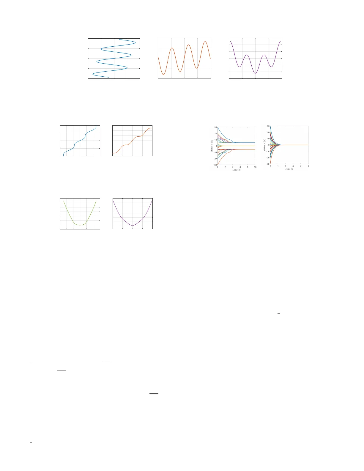
1 A Geometric Method for P assi v ation and Cooperati ve Control of Equilibrium-Independent P assi ve-Short Systems Miel Sharf, Graduate Student Member , IEEE , Anoop Jain, Member , IEEE , and Daniel Zelazo, Senior Member , IEEE Abstract —Equilibrium-independent passive-short (EIPS) sys- tems are a class of systems that satisfy a passivity-like dissipation inequality with respect to any for ced equilibria with non-positive passivity indices. This paper pr esents a geometric approach f or ﬁnding a passivizing transformation for such systems, relying on their steady-state input-output relation and the notion of projecti ve quadratic inequalities (PQIs). W e show that PQIs arise naturally from passi vity-shortage characteristics of an EIPS system, and the set of their solutions can be explicitly expressed. W e lev erage this connection to build an input-output mapping that transforms the steady-state input-output relation to a monotone relation, and show that the same mapping passivizes the EIPS system. W e show that the proposed transformation can be implemented through a combination of feedback, feed- through, post- and pre-multiplication gains. Furthermore, we consider an application of the pr esented passivation scheme for the analysis of networks comprised of EIPS systems. Numer ous examples are provided to illustrate the theoretical ﬁndings. I . I N T R O D U C T I O N Cooperativ e control has been extensiv ely studied in the last few years, as it displays both interesting theoretical questions, as well as a wide range of engineering applications [1–3]. One widespread tool in cooperativ e control is the notion of pas- sivity [3 – 5]. Passi vity theory was ﬁrst applied to multi-agent systems in [6], where it was used to solv e group coordination problems. Since then, different v ariants of passi vity were used for solving various problems in robotics [7], synchronization [8], and distributed optimization [9]. The classical notion of passivity , as appears in [10], is deﬁned with respect to equilibrium at the origin. Some authors also deﬁne shifted passi vity , which is deﬁned with respect to an input-output (I/O) pair of the system, to apply passivity-based methods to systems having forced equilibria [6, 11, 12]. For brevity , we shall not differentiate the two concepts, and refer to both as passivity . The notion of passivity with respect to a single input-output pair may not be sufﬁcient for stability analysis of multi-agent systems, as the interconnection of (shifted)-passiv e systems is stable only if the closed-loop network has an equilibrium, which can be hard to verify for networks comprised of multiple nonlinear agents having different dynamics. M. Sharf is with the Division of Decision and Control Systems, KTH Royal Institute of T echnology , Stockholm, Sweden. sharf@kth.se . A. Jain is with the Department of Electrical Engineering, Indian Institute of T echnology , Jodhpur, India. anoopj@iitj.ac.in . D. Zelazo is with the Faculty of Aerospace Engineering, Israel Institute of T echnology , Haifa, Israel dzelazo@technion.ac.il . This work was supported in part at the T echnion by Lady Davis Fello wship, and the German-Israeli Foundation for Scientiﬁc Research and Development. T o remedy this issue, sev eral variants of passivity were dev eloped, demanding systems to be passi ve with respect to any equilibrium input-output pairs or trajectories. Incremen- tal passivity [13] demands that a passiv ation inequality is held with respect to pairs of trajectories, but is often too restrictiv e. Another variant, equilibrium-independent passi vity (EIP), demands that the system is passiv e with respect to any equilibrium it has, and models the steady-state output as a continuous (monotone) function of the steady-state input [12, 14]. This variant has man y applications, e.g. [15, 16], but does not include some fundamental systems such as the single integrator , characterized by having multiple steady-state outputs for the steady-state input u = 0 (due to different initial conditions). Another variant of passi vity is maximal equilibrium-independent passivity (MEIP), introduced in [17]. Here, passi vity is assumed with respect to all equilibria, and the steady-state output is modeled as a maximally monotone relation of the steady-state input, generalizing EIP . In [17], it was shown that a diffusi vely-coupled network of SISO output- strictly MEIP agents and SISO MEIP controllers con ver ges, and its limit can be found as the minimizers of two dual con ve x network optimization problems associated with the network, usually referred to as the optimal ﬂow problem and optimal potential problem [18]. In this way , the con vex network optimization problems gi ve a computationally viable way of computing the limit of the diffusi vely-coupled netw ork. This connection was used in [19–21] to solve v arious synthesis problems, and in [22] for fault detection and isolation prob- lems. In practice, ho wev er , many systems are not passi ve [23 – 26]. Their lack of passivity is often quantiﬁed using the input- passivity index and the output-passivity index [27], and is often compensated using passiv ation methods (also known as passiﬁcation methods [28]). The goal of this paper is to present a nov el passiv ation method for systems which are not passiv e, but have a shortage of passi vity , characterized by a weaker dissipation inequality . A. Liter atur e Review The most common methods to passivize a system rely on feedback. A well-known approach is output-feedback using a ﬁxed gain [10]. This approach passivizes systems with a negati ve output-passivity index [27], otherwise kno wn as out- put passiv e-short systems. Another method considers output- feedback using a controller with prescribed passivity indices 2 [27], but passiv ation is again achiev ed only for passive- short systems [27, Theorem 7]. One can similarly consider input-feedthrough, passivizing systems with a negati v e input- passivity inde x [27], known as input-passi ve-short systems. Other prominent feedback-based methods used for passi- vation include state-feedback and output-feedback by general static nonlinearities, see [28 – 33] and references therein. These approaches were proven to work for weakly minimum phase systems with relative de gree at most 1 , but can have se veral problems. First, like L yapunov theory , these methods are often non-constructiv e, and heavily rely on structural properties of the system at hand [34, Chapter 1]. Second, the construction of the feedback law requires an e xact model of the system, or at least an approximate one. This can be a problem in cases where the model of the system changes, due to faults, wear- and-tear , unforeseen working conditions, etc. As passi vity indices can be estimated using in-run data [35–37], passiv ation methods relying on passivity indices can mitigate this ef fect by adapting the assumed passivity indices. W e also mention other methods building on state-feedback, such as backstepping and forwarding [34, Chapter 6], which remove either the minimum-phase or the relati ve-de gree requirement, but replace it with a structural assumption on the model of the system, i.e., the system must be in a triangular form. A nov el method for mitigating the problems of feedback- based methods was presented in [38]. The method considers a general I/O transformation, which deﬁnes a new input and a new output for the system as a linear combination of its original input and output. This method generalizes output- feedback and input-feedthrough with constant gains. In [38], this I/O transformation was used to passivize systems with a ﬁnite L 2 -gain. Namely , the entries of the matrix deﬁning the I/O transformation were chosen according to the L 2 -gain of the system at hand by solving a collection of equations and inequalities. In particular , the method is constructive and can successfully cope with a change in the dynamics by measuring the L 2 -gain of the new system and updating the entries of the matrix accordingly . Howe ver , the applicability of this method is limited to systems with a ﬁnite L 2 -gain, which excludes all unstable systems, input- or output-passive short systems, as well as some marginally stable systems such as the single inte grator . Thus there is a need for a more sophisticated passivization approach to deal with a wider class of systems. This motiv ates the goals of this paper . B. Contrib utions In this paper, we build on [38] and propose a nov el method for constructing passivizing I/O transformations. Our approach is based on analytic geometry , which is applicable to a wider class of systems characterized by a passivity-lik e dissipation inequality with arbitrary passivity indices. Unlike in [38], these systems need not hav e a ﬁnite L 2 -gain. W e deﬁne these systems as input-output ( ρ, ν ) -passi ve systems, including, but not restricted to, output passive-short system, input passive- short systems and ﬁnite L 2 -gain systems. W e show how to use the passivity indices of such systems to build a passi vizing I/O transformation that can be realized using an amalgamation of easily implementable components such as input-feedthrough, output-feedback, and gains. W e consider systems that are input-output ( ρ, ν ) -passi ve with respect to all forced equilibria. The collection of all these steady-state input-output pairs is known as the steady-state I/O relation of the system. The steady-state I/O relation for passiv e systems is known to be monotone [14, 17], and we show that this relation is non- monotone for passiv e-short systems. T o tackle such systems, we introduce the notion of projecti ve quadratic inequalities (PQIs), that are inequalities in two scalar variables, as well as methods inspired from analytic geometry to ﬁnd a linear transformation monotonizing 1 the steady-state relation of the system. W e then sho w that the linear transformation gi ves rise to an I/O transformation, which is sho wn to passivize the system with respect to all forced equilibria. W e further discuss an application of this passiv ation scheme for multi- agent systems, in which, the notion of MEIP leads to a network optimization framework for analysis. As we already know that the passivized systems have monotone steady-state relations, the missing key notion for assuring MEIP is maximality . In this direction, we introduce the notion of cursiv e relations to assert maximality of the monotonized relations, proving the agents are MEIP , and allowing us to deriv e a transformed network optimization framework in the spirit of [17]. W e also reproduce the results of [39] as a special case, which prov es a network optimization framework assuming the agents only hav e an output-shortage of passivity . W e exemplify our results by characterizing a class of linear and time-in variant systems as EIPS systems, and gi ve two case studies by comparing our results with the existing literature. W e emphasize that our results are also valid for classical passivity , as PQIs abstract all notions of classical passi vity discussed in the introduction. The rest of the paper is organized as follows. Section II presents some background and provides a few deﬁnitions. Section III motiv ates and formulates the problem. Section IV discusses the steady-state I/O relation of passi ve-short systems, and suggests a geometric method of ﬁnding a monotonizing transformation. Section V shows that the monotonizing trans- formation passi vizes the system, and shows how to implement the said transformation using basic control elements, such as feedback, feed-through, and gains. Section VI discusses the notion of input-output ( ρ, ν ) -passivity and its general- ity . Section VII studies the last obstacle needed for MEIP , namely maximal monotonicity , and formulates the network optimization frame work. Section VIII presents two examples of applying our methods, before we conclude the paper in Section IX. Pr eliminaries: W e use notions from graph theory [40]. A graph is a pair G = ( V , E ) , consisting of a ﬁnite set of vertices V , and a ﬁnite set of edges, E ⊂ V × V . Each edge e ∈ E consists of two vertices i, j ∈ V , and the notation e = ( i, j ) indicates that i is the head of edge e and j is its tail . The incidence matrix E ∈ R | V |×| E | of G is deﬁned such that for any edge e = ( i, j ) , [ E ] ie = +1 , [ E ] j e = − 1 , and [ E ] `e = 0 for ` 6 = i, j . The n × n identity matrix is denoted by Id n , and 0 0 0 n is the all-zero vector . The Legendre transform of a con ve x function Φ : R d → R is a function Φ ? : R d → R 1 W e introduce this word and it has the meaning of “to make monotone. ” In simple w ords, monotonizing means con verting any (non-monotone) relation to a monotone relation. 3 deﬁned by Φ ? ( y ) = sup u ∈ R d { u > y − Φ ( u ) } [41]. Moreover , the subdif ferential of a conv ex function Φ is denoted as ∂ Φ . A relation, i.e., a subset Ω ⊆ A × B of a product set, is identiﬁed with the set-valued map sending a ∈ A to { b ∈ B : ( a, b ) ∈ Ω } . Given a relation Ω ⊆ A × B , Ω − 1 denotes the inv erse relation of Ω , i.e., Ω − 1 := { ( b, a ) ∈ B × A : ( a, b ) ∈ Ω } . W e follow the conv ention that italic letters denote dynamic variables and letters in normal font denote constant signals. I I . B AC K G RO U N D This section re views the concept of MEIP , introduces sys- tems with ﬁnite equilibrium-independent passivity indices, and describes the network model for diffusi vely coupled systems. A. Maximal Equilibrium-Independent P assivity Consider the following SISO dynamical system, Υ : ˙ x = f ( x, u ); y = h ( x, u ) , (1) with state x ∈ R n , control input u ∈ R and output y ∈ R . The functions f and h are assumed to be sufﬁciently smooth. W e assume the systems in the form (1) admit forced steady- state input-output equilibrium pairs. This leads to the following deﬁnition, used extensi vely in the literature [12, 14, 17, 20]. Deﬁnition 1. The steady-state input-output relation of the system (1) is the collection of all steady-state input-output pairs (u , y) . That is, it is equal to the set k = { (u , y) : ∃ x , 0 0 0 n = f (x , u) , y = h (x , u) } . The corr esponding in verse r elation is given by k − 1 = { (y , u) : (u , y) ∈ k } . Note that any steady-state relation can be thought of as a set- valued map. Namely , for any constant input u , we can deﬁne k (u) as the set k (u) = { y : (u , y ) ∈ k } . Note that k (u) = ∅ if no steady-state output corresponding to the input u exists. Similarly , for a steady-state output y , we deﬁne k − 1 (y) as k − 1 (y) = { u : (u , y) ∈ k } , the set of all constant inputs u that can generate y . In this sense, the in verse relation can always be deﬁned, as we do not assume k to be a function. For EIP systems, it is shown in [14] that the steady-state I/O relation k is a continuous and monotonically increasing function. In particular , for any steady-state input u there is exactly one steady-state output y . Ho we ver , EIP excludes some important system classes, e.g. the single integrator [17]. T o capture the behavior of systems where the steady-state I/O relations are not necessarily a function, but rather a r elation , the notion of MEIP was suggested relying on maximal mono- tonicity of the steady-state I/O relation [17]. Deﬁnition 2. A r elation k is said to be maximal monotone if i) it is monotone, i.e., for any (u 1 , y 1 ) , (u 2 , y 2 ) ∈ k , we have that (u 2 − u 1 )(y 2 − y 1 ) ≥ 0 , and ii) it is not contained in a lar ger monotone r elation. The notion of maximal monotonicity is closely related to con ve x functions as described in the follo wing theorem. Theorem 1 ([41]) . A r elation k is maximally monotone if and only if there exists a con vex function Φ such that the subgradient ∂ Φ is equal to k . Mor eo ver , Φ is unique up to an additive constant. The function Φ is called the integral function of k . Maximal monotonicity induces the follo wing system- theoretic property: Deﬁnition 3 ([17]) . A dynamical SISO system Σ : u 7→ y is (output-strictly) maximal equilibrium independent passiv e (MEIP) if i) The system Σ is (output-strictly) passive with r espect to any steady-state I/O pair (u , y ) it possesses. ii) The associated steady-state I/O relation is maximally monotone. Examples of MEIP systems include single integrators, port- Hamiltonian systems, gradient systems, and others; see [17] for further discussion. One important aspect of MEIP systems is their integral functions, as mentioned in Theorem 1 above. Since the steady-state I/O relation k is maximally monotone for an MEIP system, there exists a con ve x function K such that ∂ K = k . Moreov er , the Le gendre transform of K , denoted as K ? , is also a conv ex function, and satisﬁes ∂ K ? = k − 1 . Thus both k , k − 1 hav e integral functions that are necessarily con ve x. Howe ver , this is not true for passi ve-short systems, as will be shown in Section III. B. Equilibrium-Independent Shortag e of P assivity The main adv antage of applying an equilibrium-independent notion of passivity for multi-agent systems is that it allows to prove con v ergence without specifying the steady-state limit (see [12, 14, 17] and Subsection II-C). Howe v er , many systems in practice are not passi ve [23 – 26], and even fewer are passi ve with respect to all equilibria. The lev el of passi vity , or shortage thereof, is usually measured using passivity indices. W e ﬁrst deﬁne the notion of shortage of passivity that we consider, and later adjust it to ﬁt into the equilibrium-independent framew ork. Deﬁnition 4. Let Σ be a SISO system with a constant input- output steady-state pair (u , y ) . The system Σ is said to be: i) output ρ -passi ve with respect to (u , y) if ther e exist a storag e function S ( x ) , and a number ρ ∈ R , such that the following inequality holds for any tr ajectory: ˙ S ≤ − ρ ( y − y) 2 + ( y − y)( u − u); (2) ii) input ν -passi ve with respect to (u , y) if there exist a storag e function S ( x ) , and a number ν ∈ R , such that the following inequality holds for any tr ajectory: ˙ S ≤ − ν ( u − u) 2 + ( y − y)( u − u); (3) iii) input-output ( ρ, ν )-passiv e with r espect to (u , y) if there exist a storag e function S ( x ) , and numbers ρ, ν ∈ R , such that ρν < 1 4 and that the following inequality holds for any trajectory: ˙ S ≤ − ρ ( y − y) 2 − ν ( u − u) 2 + ( y − y)( u − u) . (4) Remark 1. Output ρ -passive systems with ρ < 0 ar e known in the literatur e both as output-passive short or output passivity- short systems [23, 24, 39, 42–44] or as output-passiﬁable systems [45, 46]. Similarly , input ν -passive systems with ν < 0 ar e usually called input-passive short systems or as input- passiﬁable systems. 4 Deﬁnition 5. A SISO system Σ : u 7→ y is said to be: i) Equilibrium-Independent Output ρ -Passi ve (EI-OP( ρ )) if it is output ρ -passive with respect to any equilibrium. ii) Equilibrium-Independent Input ν -Passi ve (EI-IP( ν )) if it is input ν -passive with r espect to any equilibrium. iii) Equilibrium-Independent Input-Output ( ρ, ν ) -Passi ve (EI-IOP( ρ, ν )) if it is input-output ( ρ, ν )-passive with r espect to any equilibrium. Mor eover , for EI-OP( · ) and EI-IP( · ), the lar gest num- bers ρ, ν for which the inequalities (2) and (3) hold are called the equilibrium-independent output-passivity index and equilibrium-independent input-passivity index of the system, r espectively . Furthermor e, Σ is said to be equilibrium- independent passive short (EIPS) if there exist ρ, ν with ρν < 1 4 such that Σ is EI-IOP( ρ, ν ). Remark 2. The numbers ρ, ν in Deﬁnition 5 ar e not unique, as decr easing them makes the inequality easier to satisfy . W e thus deﬁne the equilibrium-independent passivity indices analogously to the output-feedback passivity index (OFP) and the input-feedthr ough passivity index (IFP) in [26]. Mor e- over , the deﬁnition above unites strictly-passive, passive, and passive-short systems. The case ρ, ν > 0 corresponds to strict passivity , ρ, ν = 0 corresponds to passivity , and ρ, ν < 0 corr esponds to shortage of passivity . Thus, it will allow us to consider networks of systems wher e some are passive and some are passive-short, without needing to specify the exact passivity assumption. It also allows us to consider EI- IOP( ρ, ν ) systems for ρ > 0 and ν < 0 (or vice versa) with no additional effort needed. Remark 3. The demand that ρν < 1 4 for deﬁning EI-IOP( ρ, ν ) might seem unnatural. The reason we add it is that otherwise, the right-hand side of (4) will either be always positive or always ne gative. The ﬁrst case implies all static nonlinearities ar e EI-IOP( ρ, ν ), and the second case implies that no system can be EI-IOP( ρ, ν ), both rendering the deﬁnition useless. Remark 4. EI-IOP( ρ, ν ) systems captur e both EI-OP( ρ ) and EI-IP( ν ) systems by setting either ρ = 0 or ν = 0 . W e now gi ve an example of a class of EI-OP( ρ ) systems: Proposition 1. Consider the SISO gradient system ˙ x = −∇ U ( x ) + u ; y = x , wher e the Hessian of the potential U satisﬁes Hess( U ) ≥ ρ Id for some ρ ∈ R . Then Σ is EI-OP( ρ ). Pr oof. T ake a steady-state I/O pair (u , y) and note x = y is the corresponding state at equilibrium. Consider the storage function S ( x ) = 1 2 k x − x k 2 . The deriv ati ve of S along the system trajectories is ˙ S = ( x − x) > ( −∇ U ( x ) + u ) . Deﬁning ϕ ( x ) := ∇ U ( x ) − ρx , we write ˙ S = ( x − x) > ( − ϕ ( x ) − ρx + u ) . Adding and subtracting ϕ (x) and ρ x and using the fact that u = ∇ U (x) , y = x and ϕ (x) = ∇ U (x) − ρ x at equilibrium, we obtain ˙ S = − ( x − x) > (( ϕ ( x ) − ϕ (x)) − ρ ( y − y) > ( y − y) + ( y − y)( u − u)) . It is straightforward to verify that Hess( U ) ≥ ρ Id implies that ∇ ϕ ( x ) ≥ 0 , so ϕ ( · ) is a monotone operator , that is, − ( x − x) > (( ϕ ( x ) − ϕ (x)) ≤ 0 . W e thus conclude that ˙ S ≤ − ρ ( y − y) > ( y − y) + ( y − y) > ( u − u)) , and hence the system is EI-OP( ρ ). E E T ζ ( t ) µ ( t ) u ( t ) y ( t ) Σ 1 Σ 2 Σ | V | . . . Π 1 Π 2 Π | E | . . . Fig. 1. A dif fusiv ely-coupled network. C. Dif fusively-Coupled Network Model W e consider a collection of SISO agents interacting over a network G = ( V , E ) , in which the agents reside at the nodes V , and the edges regulate the relative output between the associated nodes. Namely , the agents { Σ i } i ∈ V and the controllers { Π e } e ∈ E hav e the following models: Σ i : ( ˙ x i = f i ( x i , u i ) y i = h i ( x i , u i ) , Π e : ( ˙ η e = φ e ( η e , ζ e ) µ e = ψ e ( η e , ζ e ) , (5) where x i ∈ R ` i , η e ∈ R ` e are the states, u i , ζ e ∈ R are the inputs and y i , µ e are the outputs. W e deﬁne the stacked vectors u u u = [ u 1 , · · · , u | V | ] > , and similarly for x x x, y y y , ζ ζ ζ , η η η and µ µ µ . The agents and controllers are coupled by ζ ζ ζ = E > y y y and u u u = −E µ µ µ , where E is the incidence matrix of G . The closed-loop system is called the diffusively-coupled system ( Σ Σ Σ , Π Π Π , G ) , and the associated block-diagram can be seen in Figure 1. Dif fusiv ely- coupled networks are of considerable interest in the control literature [6, 17, 47], and include important examples such as neural networks [48], the Kuramoto model for oscillator synchronization [49], and trafﬁc control models [50]. The notion of MEIP allows us to connect between diffusi v ely-coupled networks and network optimization theory . Theorem 2 ([17]) . Consider the diffusively-coupled system ( Σ Σ Σ , Π Π Π , G ) . Suppose the agents are output-strictly MEIP and the contr ollers ar e MEIP , or vice versa. Let K i be the agents’ inte gral functions, and let Γ e be the contr oller s’ inte gral func- tions. W e denote K K K ( u u u) = P i ∈ V K i (u i ) , Γ Γ Γ( µ µ µ ) = P e ∈ E Γ i ( µ i ) , and similarly for the Le gendr e transforms. Then ther e exist constant vector s u u u , y y y , ζ ζ ζ , µ µ µ such the signals u u u ( t ) , y y y ( t ) , ζ ζ ζ ( t ) , µ µ µ ( t ) of ( Σ Σ Σ , Π Π Π , G ) asymptotically con verg e to u u u , y y y , ζ ζ ζ , µ µ µ corr espond- ingly . Moreo ver , the steady-states u u u , y y y , ζ ζ ζ and µ µ µ ar e (dual) so- lutions of the following pair of conve x optimization pr oblems: OFP OPP min u u u , µ µ µ K K K ( u u u) + Γ Γ Γ ? ( µ µ µ ) s.t. u u u = −E µ µ µ . min y y y , ζ ζ ζ K K K ? ( y y y) + Γ Γ Γ( ζ ζ ζ ) s.t. E > y y y = ζ ζ ζ These static optimization problems are known as the Opti- mal Flow Pr oblem (OFP) and the Optimal P otential Pr oblem (OPP) , and are dual to each other . These are classical problems in the mathematical ﬁeld of network optimization, dealing with static optimization problems deﬁned on graphs, and hav e been extensi vely studied by various researchers in ﬁelds as theoretical computer science and operations research [18]. Howe v er , this frame work heavily relies on the passi vity of the agents and controllers, and fails if any of the agents are 5 not MEIP . As we’ll see later, if the agents are not passiv e, the integral functions might be non-conv ex, or may not even exist. I I I . M OT I V A T I O N A N D P RO B L E M F O R M U L A T I O N Our end-goal is to extend the network optimization frame- work of Theorem 2 to agents which are not MEIP , but are rather EIPS. Unlike MEIP systems, EIPS systems need not hav e monotone steady-state relations. In some cases, this lack of monotonicity results in the non-con v exity of the corresponding integral function [39], and in other cases, the steady-state I/O relation is far enough from monotone that an integral function cannot ev en be deﬁned. W e giv e examples of this phenomenon in the following: Example 1 (EI-OP( ρ )) . Consider a SISO system ˙ x = − x + 3 √ x + u ; y = 3 √ x . It is shown in [39] that this system is EI-OP( ρ ) for all ρ ≤ − 1 , and its equilibrium-independent passivity index is ρ = − 1 . Mor eover , the in verse steady- state I/O relation u = k − 1 (y) = y 3 − y is not monotone. Furthermor e, it has an inte gral function K ? (y) = 1 4 y 4 − 1 2 y 2 , which is non-con ve x due to the negative quadr atic term. Example 2 (EI-IP( ν )) . Consider the SISO system ˙ x = − 3 √ x + u ; y = x − u . One can show similarly to Example 1 that this system is EI-IP( ν ) for all ν ≤ − 1 , and ν = − 1 is its equilibrium-independent passivity index. Mor eover , the steady- state I/O relation y = k (u) = u 3 − u is not monotone. Furthermor e, it has an integr al function K (u) = 1 4 u 4 − 1 2 u 2 , which is again non-con ve x due to the ne gative quadratic term. Example 3 (EI-IOP( ρ, ν )) . Consider a SISO dynamical system Σ given by Σ : ˙ x = − 3 √ x + 0 . 5 x + 0 . 5 u ; y = 0 . 5 x − 0 . 5 u, (8) with input u and output y . F or any steady-state input-output pair (u , y) and the corresponding state at equilibrium x = 2y+ u , we can consider the stor age function S ( x ) = 1 6 ( x − x) 2 . A simple calculation shows that: ˙ S ≤ ( u − u)( y − y) + 1 3 ( u − u) 2 + 2 3 ( y − y) 2 , meaning that the system is EI-IOP( ρ, ν ) for ρ = − 2 / 3 and ν = − 1 / 3 . One can also easily verify that given an equilibrium state x , the steady-state input u is given by u = 2 3 √ x − x and that the steady-state output is y = x − 3 √ x . Deﬁning σ = − 3 √ x , we see that the steady-state r elation of the system is given by the planar curve u = 2 σ − σ 3 ; y = σ 3 − σ , par ameterized by a variable σ , as shown in F igur e 2. It is clear fr om F igur e 2 that both steady-state I/O relation and its in verse are non- monotone. In fact, the steady-state input-output relation and its in verse ar e so far fr om monotone, no inte gral function e xists for either of them. However , if we deﬁne a new input ˜ u and a new output ˜ y by ˜ u = u + y, ˜ y = u + 2 y , the r esulting loop tr ansformation gives the following system: ˜ Σ : ˙ x = − 3 √ x + ˜ u ; ˜ y = x, (9) which has the steady-state input-output r elation k ( ˜ u) = u 3 , which is maximally monotone. Mor eover , the system (9) can be veriﬁed to be MEIP with storage function S ( x ) = 1 2 ( x − x) 2 . -2 -1.5 -1 -0.5 0 0.5 1 1.5 2 Input (u) -4 -3 -2 -1 0 1 2 3 4 Output (y) (a) The steady-state relation of (8). -4 -3 -2 -1 0 1 2 3 4 Output (y) -2 -1.5 -1 -0.5 0 0.5 1 1.5 2 Input (u) (b) The in verse relation of (8). Fig. 2. Steady-state relations of the system in Example 3. The abov e example shows that EIPS systems need not hav e integral functions, nor (maximally) monotone steady- state I/O relations. Thus, the netw ork optimization frame work of [17] cannot even be deﬁned for networks of EIPS agents. In [39, 44], the network optimization framework failed due to the lack of con vexity of the integral functions. This was remedied by con vexifying the resulting (non-conv ex) network optimization problems. The interpretation (or implementation) of this conv exiﬁcation was a passi vizing feedback term. W e cannot follow this idea for EIPS systems when ρ, ν < 0 , as the network optimization framew ork is not even deﬁned. More- ov er , diffusely-coupled networks consisting of such systems might not be stable. T o ov ercome these shortcomings for EIPS systems, we inv estigate the existence of a loop transformation which results in monotonizing the steady-state I/O relation of the agents, as illustrated in the last part of Example 3. Thus, our goal in this paper is to ﬁnd a monotonizing procedure for the steady-state I/O relation. W e further sho w that the mono- tonizing procedure induces a passivizing plant transformation. For the rest of this paper, let Σ be a EI-IOP( ρ, ν ) system for known parameters ρ, ν , and let k be the corresponding steady- state relation. I V . M O N OT O N I Z AT I O N O F I / O R E L A T I O N S B Y L I N E A R T R A N S F O R M AT I O N S : A G E O M E T R I C A P P ROA C H Our goal is to ﬁnd a monotonizing transformation T : (u , y) 7→ (˜ u , ˜ y) for k . W e look for a linear transformation T of the form  ˜ u ˜ y  = T [ u y ] . Assuming the system is EI-IOP( ρ, ν ) allows us to deduce information about the steady-state I/O relation: Proposition 2. Let Σ be an EI-IOP( ρ, ν ) system and let k be its steady-state I/O r elation. Then for any two points (u 1 , y 1 ) , (u 2 , y 2 ) in k , the following inequality holds: 0 ≤ − ρ (y 1 − y 2 ) 2 + (u 1 − u 2 )(y 1 − y 2 ) − ν (u 1 − u 2 ) 2 . (10) Pr oof. By deﬁnition of EI-IOP( ρ, ν ), (4) holds for any steady- state (u , y) and any trajectory ( u ( t ) , x ( t ) , y ( t )) . Considering the steady-state (u 1 , y 1 ) , we conclude that there e xists a positiv e-deﬁnite storage function S ( x ) such that the follo wing inequality holds for all trajectories ( u ( t ) , x ( t ) , y ( t )) : dS dt ≤ − ρ ( y − y 1 ) 2 − ν ( u − u 1 ) 2 + ( y − y 1 )( u − u 1 ) . (11) The steady-state input-output pair (u 2 , y 2 ) corresponds to some steady state x 2 , so that (u 2 , x 2 , y 2 ) is an (equilibrium) 6 trajectory of the system. Plugging it into (11), and noting that d dt S (x 2 ) = 0 , we conclude that the inequality (10) holds. Proposition 2 suggests the following deﬁnition: Deﬁnition 6. A projecti ve quadratic inequality (PQI) is an inequality with variables ξ , χ ∈ R of the form 0 ≤ aξ 2 + bξ χ + cχ 2 , (12) for some numbers a, b, c , not all zer o. The inequality is called non-trivial if b 2 − 4 ac > 0 . The associated solution set of the PQI is the set of all points ( ξ , χ ) ∈ R 2 satisfying the inequality . By Deﬁnition 6, it is clear that (10) is a PQI. Indeed, plugging ξ = u 1 − u 2 , χ = y 1 − y 2 and choosing a, b, c correctly veriﬁes this. The demand ρν < 1 4 is equiv alent to the non-triviality of the PQI. For example, monotonicity of the steady-state k can be written as 0 ≤ (u 1 − u 2 )(y 1 − y 2 ) , which can be transformed to a PQI by choosing a = c = 0 and b = 1 in (12). Similarly , strict monotonicity can be modeled by taking b = 1 and a ≤ 0 , c < 0 . As for transformations, the transformation T =  T 11 T 12 T 21 T 22  of the form  ˜ u ˜ y  = T [ u y ] can be written as ˜ u = T 11 u + T 12 y and ˜ y = T 21 u + T 22 y . Plugging it inside (10) gives another PQI. More precisely , if we let F ( ξ , χ ) = aξ 2 + bξ χ + cχ 2 , and T is a linear map, then T maps the PQI F ( ξ , χ ) ≥ 0 to F ( T − 1 ( ˜ ξ , ˜ χ )) ≥ 0 . Our goal is to ﬁnd a map T transforming the inequality in Deﬁnition 6 to the PQI corresponding to monotonicity . Thus, we are compelled to consider the action of the group of linear transformations on the collection of PQIs. Let A be the solution set of the original PQI. The connection between the original and transformed PQI described abo ve shows that the solution set of the ne w PQI is T ( A ) = { T ( ξ , χ ) : ( ξ , χ ) ∈ A} . W e can therefore study the effect of linear transformations on PQIs by studying their actions on the solution sets. The action of the group of linear transformations on the collection of PQIs can be understood algebraically , but we use solution sets to understand it geometrically . W e ﬁrst giv e a geometric characterization of the solution sets. Note 1. In this section, we abuse notation and identify the point (cos θ , sin θ ) on the unit circle S 1 with the angle θ in some se gment of length 2 π . Deﬁnition 7. A symmetric section S on the unit circle S 1 ⊆ R 2 is the union of two closed disjoint sections that ar e opposite to each other , i.e., S = B ∪ ( B + π ) where B is a closed section of angle < π . A symmetric double-cone is deﬁned as A = { λs : λ > 0 , s ∈ R } for a symmetric section S . An example of a symmetric section and the associated symmetric double-cone can be seen in Figure 3. Theorem 3. The solution set of any non-trivial PQI is a symmetric double-cone. Moreo ver , any symmetric double-cone is the solution set of some non-trivial PQI, which is unique up to a positive multiplicative constant. The proof of the theorem is a vailable in the appendix. The theorem presents a geometric interpretation of the steady-state condition (10). The connection between cones and measures of passivity is best kno wn for static systems through the notion -1 -0.5 0 0.5 1 -1 -0.8 -0.6 -0.4 -0.2 0 0.2 0.4 0.6 0.8 1 Fig. 3. A double cone (in blue), and the associated symmetric section S (in solid red). The parts of S 1 outside S are presented by the dashed red line of sector-bounded nonlinearities [10]. It was expanded to more general systems in [51], and later in [52]. W e consider a different branch of this connection, focusing on the steady- state relation rather on trajectories. In turn, it allows us to ha ve intuition when constructing monotonizing maps. In particular , we hav e the following result. Theorem 4. Let ( ξ 1 , χ 1 ) , ( ξ 2 , χ 2 ) be two non-colinear solu- tions of a 1 ξ 2 + ξ χ + c 1 χ 2 = 0 . Moreo ver , let ( ξ 3 , χ 3 ) , ( ξ 4 , χ 4 ) be two non-colinear solutions of a 2 ξ 2 + ξ χ + c 2 χ 2 = 0 . Deﬁne T 1 =  ξ 3 ξ 4 χ 3 χ 4   ξ 1 ξ 2 χ 1 χ 2  − 1 , T 2 =  ξ 3 − ξ 4 χ 3 − χ 4   ξ 1 ξ 2 χ 1 χ 2  − 1 . (13) Then one of T 1 , T 2 transforms the PQI a 1 ξ 2 + ξ χ + c 1 χ 2 ≥ 0 to the PQI τ a 2 ξ 2 + τ ξ χ + τ c 2 χ 2 ≥ 0 for some τ > 0 . The non-colinear solutions correspond to the straight lines forming the boundary of the symmetric double-cone, thus can be found geometrically . Moreo ver , as will be evident from the proof, kno wing which one of T 1 and T 2 works is possible by checking the PQIs on ( ξ 1 + ξ 2 , χ 1 + χ 2 ) and ( ξ 3 + ξ 4 , χ 3 + χ 4 ) . Namely , if exactly one of them satisﬁes the PQIs, then T 2 works, and otherwise T 1 works. W e know present the proof of the theorem. Pr oof. Let A 1 be the solution set of the ﬁrst PQI, and let A 2 be the solution set of the second PQI. W e sho w that either T 1 or T 2 maps A 1 to A 2 . W e note that T 1 ( A 1 ) and T 2 ( A 1 ) are symmetric double-cones, whose boundary is the image of the boundary of A 1 under T 1 and T 2 respectiv ely , i.e., they are the image of span { ( ξ 1 , χ 1 ) } ∪ span { ( ξ 2 , χ 2 ) } under T 1 , T 2 . W e note that T 1 maps ( ξ 1 , χ 1 ) , ( ξ 2 , χ 2 ) to ( ξ 3 , χ 3 ) , ( ξ 4 , χ 4 ) correspondingly , and that T 2 maps ( ξ 1 , χ 1 ) , ( ξ 2 , χ 2 ) to ( ξ 3 , χ 3 ) , ( − ξ 4 , − χ 4 ) correspondingly . Thus, span { ( ξ 1 , χ 1 ) } ∪ span { ( ξ 2 , χ 2 ) } is mapped by T 1 and T 2 to span { ( ξ 3 , χ 3 ) } ∪ span { ( ξ 4 , χ 4 ) } , so that T 1 ( A 1 ) , T 2 ( A 1 ) ha ve the same bound- ary as A 2 . Since T 1 , T 2 are homeomorphisms, they map interior points to interior points. Thus, it’ s enough to show that some point in the interior of A 1 is mapped to a point in A 2 either by T 1 or by T 2 , or equiv alently , that a point in the interior of R 2 \ A 1 is mapped to a point in R 2 \ A 2 either by T 1 or by T 2 . Consider the point ( ξ 1 + ξ 2 , χ 1 + χ 2 ) . By non-colinearity , this point cannot be on the boundary of A 1 , equal to span { ( ξ 1 , χ 1 ) } ∪ span { ( ξ 2 , χ 2 ) } . Hence, it’ s either in the interior of A 1 or in the interior of its complement. W e assume the prior case, as the proof for the other is similar . The point ( ξ 1 + ξ 2 , χ 1 + χ 2 ) is mapped to ( ξ 3 ± ξ 4 , χ 3 ± χ 4 ) by T 1 , T 2 . 7 By non-colinearity , these points do not lie on the boundary of A 2 . Moreov er , the line passing through them is parallel to span { ( ξ 4 , χ 4 ) } which is part of the boundary of A 2 , and their average is ( ξ 3 , χ 3 ) , which is on the boundary . Thus, one point is in the interior of A 2 , and one is in the interior of its complement. This completes the proof. Example 4. Consider the system Σ studied in Example 3, in which the steady-state I/O relation was non-monotone. Ther e, we saw that the system is EI-IOP( ρ, ν ) with parameter s ρ = − 2 / 3 and ν = − 1 / 3 . The corr esponding PQI is 0 ≤ 1 3 ξ 2 + ξ χ + 2 3 χ 2 . W e use Theor em 4 to ﬁnd a monotonizing transformation. That is, we seek a tr ansformation mapping the given PQI to the PQI deﬁning monotonicity , ξ χ ≥ 0 . W e take ( ξ 3 , χ 3 ) = (1 , 0) and ( ξ 4 , χ 4 ) = (0 , 1) , as these ar e non-colinear solutions to ξ χ = 0 . F or the original PQI, 0 = 1 3 ξ 2 + ξ χ + 2 3 χ 2 can be r ewritten as 1 3 ( ξ + χ )( ξ + 2 χ ) = 0 , so we take ( ξ 1 , χ 1 ) = (2 , − 1) and ( ξ 2 , χ 2 ) = ( − 1 , 1) . It’ s easy to check that ( ξ 1 + χ 1 , ξ 2 + χ 2 ) = (1 , 0) satisﬁes the original PQI 0 ≤ 1 3 ξ 2 + ξ χ + 2 3 χ 2 , and that ( ξ 3 + χ 3 , ξ 4 + χ 4 ) satisﬁes ξ η ≥ 0 so the map T 1 deﬁned in the Theor em 4, should monotonize the steady-state relation. Plugging in T 1 , we get  ξ χ  = T − 1 1 h ˜ ξ ˜ χ i for T 1 = [ 1 0 0 1 ]  2 − 1 − 1 1  − 1 = [ 1 1 1 2 ] , so that T − 1 1 =  2 − 1 − 1 1  . Then, 0 ≤ 1 3 ξ 2 + ξ χ + 2 3 χ 2 = 1 3 (2 ˜ ξ − ˜ χ ) 2 + (2 ˜ ξ − ˜ χ )( − ˜ ξ + ˜ χ ) + 2 3 ( − ˜ ξ + ˜ χ ) 2 = 1 3 ˜ ξ ˜ χ, so the transformed PQI is 0 ≤ ˜ ξ ˜ χ , corr esponding to mono- tonicity . T o get the transformed steady-state r elation, we r ecall that the steady-state r elation of Σ is given by the planar curve u = 2 σ − σ 3 ; y = σ 3 − σ , parameterized by a variable σ . The transformed r elation is given by:  ˜ u ˜ y  = T 1  u y  =  1 1 1 2   2 σ − σ 3 σ 3 − σ  =  σ σ 3  , and can be modeled as ˜ y = ˜ u 3 , which is a monotone relation. Theorem 4 prescribes a monotonizing transformation for the relation k . Moreo ver , it prescribes a transformation forcing strict monotonicity , which can be viewed as the PQI − ν ξ 2 + ξ χ ≥ 0 for ν ≥ 0 , which are not both zero. V . F RO M M O N OT O N I Z AT I O N T O P A S S I V A T I O N A N D I M P L E M E N T A T I O N Until now , we found a map T : R 2 → R 2 , monotonizing the steady-state relation k . W e claim T , in fact, transforms the agent Σ into a system which is passi ve with respect to all equilibria, by deﬁning a new input and output as  ˜ u ˜ y  = T [ u y ] . Proposition 3. Let Σ be EI-IOP( ρ, ν ), and let T be a map transforming the PQI − ν ξ 2 + ξ χ − ρχ 2 ≥ 0 to − ν 0 ξ 2 + ξ χ − ρ 0 χ 2 ≥ 0 as in Theor em 4. Consider the transformed system ˜ Σ with input and output  ˜ u ˜ y  = T [ u y ] . Then ˜ Σ is EI-IOP( ρ 0 , ν 0 ). In particular , if T monotonizes the r elation k , it passivizes Σ . Pr oof. The inequality (4) is the PQI − ν ξ 2 + ξ χ − ρχ 2 ≥ 0 , where we put ξ = u ( t ) − u and χ = y ( t ) − y for a trajectory ( u ( t ) , y ( t )) and a steady-state I/O pair (u , y) . The proposition follows by noting that  ξ χ  = T − 1 h ˜ ξ ˜ χ i , satisﬁes the PQI − ν 0 ξ 2 + ξ χ − ρ 0 χ 2 ≥ 0 , ˜ ξ = ˜ u ( t ) − ˜ u and ˜ χ = ˜ y ( t ) − ˜ y . Combining Theorem 4 and the discussion follo wing it with Proposition 3 giv es the following algorithm for passiv ation of EI-IOP( ρ, ν ) systems with respect to all equilibria: Algorithm 1 Passi v ation of an EI-IOP( ρ, ν ) system Input : A system Σ , and ρ, ν ∈ R such that the system is EI-IOP( ρ, ν ). T wo more numbers ρ 0 , ν 0 such that ρ 0 ν 0 < 1 / 4 . Output : A transformation T , transforming the system Σ to an EI-IOP( ρ 0 , ν 0 ) system. 1: Find two pairs ( ξ 1 , χ 1 ) , ( ξ 2 , χ 2 ) , which are non-colinear solutions of − ν ξ 2 + ξ χ − ρχ 2 = 0 . 2: Find two pairs ( ξ 3 , χ 3 ) , ( ξ 4 , χ 4 ) , which are non-colinear solutions of − ν 0 ξ 2 + ξ χ − ρ 0 χ 2 = 0 . 3: Deﬁne T 1 , T 2 as in (13). 4: Deﬁne α 1 = − ν ( ξ 1 + ξ 2 ) 2 + ( ξ 1 + ξ 2 )( χ 1 + χ 2 ) − ρ ( χ 1 + χ 2 ) 2 and α 2 = − ν 0 ( ξ 3 + ξ 4 ) 2 + ( ξ 3 + ξ 4 )( χ 3 + χ 4 ) − ρ 0 ( χ 3 + χ 4 ) 2 . 5: if α 1 , α 2 are both non-positiv e or both non-negati ve, then 6: Return T 1 . 7: else 8: Return T 2 . 9: end if Remark 5. Proposition 3, tog ether with Section IV, prescribes a linear transformation passivizing the agent with r espect to all equilibria. The same pr ocedur e can be applied to “classi- cal” passivity , in which one only looks at passivity with r espect to a single equilibrium, as PQIs can be used to abstr actify all dissipation inequalities. Our appr oach is entirely geometric and does not rely on algebr aic manipulations. Remark 6. Note that if the tr ansformation transforms k to a strictly monotone r elation, the transformed system is strictly passive. For the remainder of this section, we show that the I/O transformation can be easily implemented using standard control tools, namely gains, feedback and feed-through. W e also connect the steady-state I/O relation λ of the transformed system ˜ Σ to k . In this direction, take any linear map T : R 2 → R 2 of the form T =  a b c d  , where we assume that det( T ) 6 = 0 . It deﬁnes the plant transformation of the form  ˜ u ˜ y  = T [ u y ] . F or simplicity of presentation, we assume that a 6 = 0 . 2 W e note T can be written as a product of elementary matrices, and the ef- fect of each elementary matrix on Σ can be easily understood. By applying the elementary transformations sequentially , the effect of their product, T , can be realized. T able I summarizes the elementary transformations and their ef fect on the system Σ . Follo wing T able I, T is written as T =  a b c d  =  δ D 0 0 1  | {z } L D  1 0 δ C 1  | {z } L C  1 0 0 δ B  | {z } L B  1 δ A 0 1  | {z } L A , (14) 2 W e note that by switching the names of ( ξ 3 , χ 3 ) and ( ξ 4 , χ 4 ) in Theorem 4, we switch the two columns of T . Thus we can always assume that a 6 = 0 , as a = b = 0 cannot hold due to the determinant condition. 8 T ext Fig. 4. The transformed system ˜ Σ after the linear transformation T . If T =  a b c d  , then δ A = b/a, δ B = d − b a c, δ C = c and δ D = a . with δ A = b/a, δ B = d − b a c, δ C = c and δ D = a . The product of these matrices can be seen as the sequential transformation from the original system Σ , which can be understood as a loop-transformation, illustrated in Figure 4. Remark 7. Writing T = L D L C L B L A allows us to give a closed form description of the tr ansformed system. Suppose the original system is given by ˙ x = f ( x, u ); y = h ( x ) . Applying L A gives a new input v , and the transformed system ˙ x = f ( x, v − δ A h ( x )); y = h ( x ) . Applying L B on this system gives ˙ x = f ( x, v − δ A h ( x )); y = δ B h ( x ) . Applying L C then gives ˙ x = f ( x, v − δ A h ( x )); y = δ B h ( x ) + δ C v , and applying L D ﬁnally gives ˙ x = f ( x, δ D v − δ A h ( x )); y = δ B h ( x ) + δ C δ D v . Proposition 4. Let k and λ be the steady-state I/O r elations of Σ and ˜ Σ , respectively , wher e ˜ Σ is the r esult of applying the transformation T in (14) on Σ , wher e δ A = b/a, δ B = d − b a c, δ C = c and δ D = a . Assume that κ 1 is the steady- state I/O relation for the system Σ 1 : u 1 7→ y 1 , obtained after the transformation L A =  1 δ A 0 1  on the original system Σ . Then, the r elation between λ and k is given by λ ( ˜ u) =  d − b a c  κ 1  1 a ˜ u  + c a ˜ u , (15) wher e the in verse of κ 1 is ( κ 1 ) − 1 (y 1 ) = k − 1 (y 1 ) + b a y 1 . (16) Pr oof. Denote the steady-state I/O relations after the ﬁrst, sec- ond, and third elementary matrix transformations, sequentially in (14), as κ 1 , κ 2 , κ 3 , corresponding to the steady-state I/O pairs (u 1 , y 1 ) , (u 2 , y 2 ) and (u 3 , y 3 ) . The transformation  u 1 y 1  = L A  u y  =  1 b/a 0 1   u y  , has the steady-state in verse I/O relation κ − 1 1 (y 1 ) = k − 1 (y 1 ) + b a y 1 . The second transformation  u 2 y 2  = L B  u 1 y 1  =  1 0 0 d − bc/a   u 1 y 1  , has the steady-state I/O relation κ 2 (u 2 ) = ( d − b a c ) κ 1 (u 2 ) . The third transformation  u 3 y 3  = L C  u 2 y 2  =  1 0 c 1   u 2 y 2  , has steady-state I/O relation κ 3 (u 3 ) = κ 2 (u 3 ) + c u 3 . Finally ,  ˜ u ˜ y  = L D  u 3 y 3  =  a 0 0 1   u 3 y 3  , has the steady-state I/O relation λ of ˜ Σ , and λ ( ˜ u) = κ 3 ( 1 a ˜ u) . Substituting back for κ 3 and for κ 2 , we get the result. Example 5. Consider the system in Examples 3 and 4. The steady-state I/O r elation λ of ˜ Σ consists of all pairs ( ˜ u , ˜ u 3 ) . W e use Pr oposition 4 to verify this r esult. Accor ding to Pr oposition 4, for the given matrix tr ansformation T = [ 1 1 1 2 ] , λ is given by λ (˜ u) = κ 1 ( ˜ u) + ˜ u . After the ﬁrst tr ansformation L A = [ 1 1 0 1 ] , the steady-state I/O pairs of the system Σ 1 ar e u 1 = u + y , and y 1 = y . Substituting u = 2 σ − σ 3 , and y = σ 3 − σ as obtained in Example 3 yields u 1 = σ and hence κ 1 (u 1 ) = y 1 = u 3 1 − u 1 . This implies that κ 1 ( ˜ u 1 ) = u 3 1 − u 1 , which on substitution yields λ ( ˜ u) = ˜ u 3 , as expected. As discussed above, in some cases, i.e., when ρ, ν ≥ 0 , we know the original system possesses inte gral functions. W e can integrate (15) and (16), obtaining a connection between the original and the transformed inte gral functions. F or exam- ple, integrating the steady-state equation for output-feedback λ − 1 (˜ y ) = k − 1 (˜ y ) + δ ˜ y results in K ? (˜ y ) = Λ ? (˜ y ) + δ 2 ˜ y 2 , where K ? , Λ ? are the integral functions of k − 1 , λ − 1 respectiv ely . Similarly , input-feedthrough corresponds to a quadratic term added to the integral function K of k , and pre- and post-gain correspond to scaling the inte gral function. These connections are summarized in T able I. Example 6. Consider Example 1. The steady-state input- output relation for the system is u = k − 1 (y) = y 3 − y , so the corr esponding inte gral function is K ? (y) = 1 4 y 4 − 1 2 y 2 . Consider the transformation T = [ 1 1 0 1 ] , or equivalently ˜ u = u + y = u + 3 √ x, ˜ y = y , so u = − 3 √ x + ˜ u . The transformed system ˜ Σ has the state-space model ˙ x = − x + ˜ u, ˜ y = 3 √ x , which has a steady-state I/O r elation of ˜ u = λ − 1 (˜ y ) = ˜ y 3 , and corr esponding inte gral function is Λ ? (˜ y ) = 1 4 ˜ y 4 . It is evident that Λ ? (y) = K ? (y) + 1 2 y 2 , as for ecasted by T able I. The passiv ation results achiev ed up to now assumed that the system at hand is EIPS. In the next section, we connect this property to having a ﬁnite L 2 -gain, showing our results extend [38]. V I . F I N I T E L 2 - G A I N A N D I N P U T - O U T P U T P A S S I V I T Y This section establishes a connection between the notion of input-output ( ρ, ν ) -passi vity and the ﬁnite L 2 -gain property , and compares our results with the existing literature. W e further explore these connections for the special case of linear and time-in v ariant systems and draw some important conclusions. A. F inite L 2 -gain and Input-Output ( ρ, ν ) -P assivity W e begin with by recalling the deﬁnition of systems with ﬁnite L 2 -gain. Deﬁnition 8. The system Σ : u 7→ y has ﬁnite- L 2 -gain with r espect to the steady-state I/O pair (u , y ) if ther e e xists some β > 0 and a storage function S such that: ˙ S ≤ − ( y − y) > ( y − y) + β 2 ( u − u) > ( u − u) . (17) The smallest number β satisfying the dissipation inequality is called the L 2 -gain of the system Σ . 9 T ABLE I E L EM EN T A RY M ATR I C E S A N D T H E I R R E AL IZ A T I O NS Elementary T ransformation Relation between I/O of Σ and ˜ Σ Effect on Steady-State Relations Realization Effect on Integral Functions L A =  1 δ A 0 1  ˜ u = u + δ A y ˜ y = y λ − 1 A (˜ y) = k − 1 (˜ y) + δ A ˜ y output- feedback Λ ? (y) = K ? (y) + 1 2 δ A y 2 L B =  1 0 0 δ B  ˜ u = u ˜ y = δ B y λ B (u) = δ B k (u) or λ − 1 B (˜ y) = k − 1 ( 1 δ B ˜ y) post-gain Λ ? (y) = 1 δ B K ? ( 1 δ B y) or Λ(u) = δ B K (u) L C =  1 0 δ C 1  ˜ u = u ˜ y = y + δ C u λ C (˜ u) = k ( ˜ u) + δ C ˜ u input- feedthrough Λ(u) = K (u) + 1 2 δ C u 2 L D =  δ D 0 0 1  ˜ u = δ D u ˜ y = y λ − 1 D (y) = δ D k − 1 (y) or λ D (˜ u) = k ( 1 δ D ˜ u) pre-gain Λ ? (y) = δ D K ? (y) or Λ(u) = 1 δ D K ( 1 δ D u) The notion of systems with a ﬁnite L 2 -gain can also be understood using the operator norm, namely , a system Σ : u 7→ y has a ﬁnite L 2 -gain if and only if its induced operator norm sup u 6 =0 k Σ( u ) k k u k is ﬁnite. In that case, the L 2 -gain is equal to the operator norm [10]. W e now show that any system with a ﬁnite L 2 -gain is actually input passiv e-short, and thus included in the collection of input-output ( ρ, ν ) -passi ve systems. Theorem 5. Let Σ : u 7→ y be any ﬁnite L 2 -gain system with r espect to the steady-state input-output pair (u , y ) with gain β . Then Σ is input ν -passive with r espect to (u , y) , in the sense of Deﬁnition 5, where ν ≤ −  β 2 + 1 4  . Pr oof. Let S ( x ) be the storage function corresponding to the ﬁnite L 2 -gain system Σ . By assumption, we know that for any trajectory ( u ( t ) , x ( t ) , y ( t )) , the follo wing inequality holds: dS dt ( x ) ≤ −k y ( t ) − y k 2 + β 2 k u ( t ) − u k 2 . W e note that k y ( t ) − y + 0 . 5( u ( t ) − u) k 2 ≥ 0 , implying that −k y ( t ) − y k 2 ≤ ( u ( t ) − u) > ( y ( t ) − y) + 0 . 25 k u ( t ) − u k 2 . Thus, we conclude that dS dt ( x ) ≤ −k y ( t ) − y k 2 + β 2 k u ( t ) − u k 2 ≤ ( u ( t ) − u) > ( y ( t ) − y) +  β 2 + 1 4  k u ( t ) − u k 2 , implying that Σ is input ν -passi ve with respect to (u , y ) . This concludes the proof of the claim. Remark 8. One can easily c heck that the above r esult is not true in the opposite dir ection, that is, if the system Σ is EI- IP( ν ) for some ν , it does not necessarily have a ﬁnite L 2 -gain. Thus, the consideration of EIPS system is more general when compar ed to ﬁnite- L 2 -gain systems as in [38]. Subsection VIII-A gives an example of a system whic h is EIPS but neither input passive-short, output passive-short, nor does it have a ﬁnite L 2 -gain. Remark 9. Systems with a ﬁnite L 2 -gain have in important use in appr oximation theory . In many examples, we do not have an exact model for a system Σ , but instead we ar e given a model for an appr oximate model Σ 0 and a bound on the appr oximation err or Σ − Σ 0 , usually in terms of its L 2 - gain. In this case, pr oving that Σ 0 satisﬁes some dissipation inequality might be easy , but trying to directly ﬁnd such an inequality satisﬁed by Σ can be an arduous task. However , [53] describes a method to pr ove a dissipation inequality for Σ using a dissipation inequality for Σ 0 and an estimate on the L 2 -gain of the appr oximation err or Σ − Σ 0 . The achie ved dissipation inequality might be very conservative, b ut we can still apply Algorithm 1, as it does not need the e xact passivity indices, but only some bound on them. In particular , the pr esented appr oach works even when we are only given an appr oximation of the true system. B. Equilibrium-Independent P assive Shortage and Linear and T ime-In variant Systems This subsection dri ves an important result for the linear and time-in v ariant systems (L TI) relating their transfer function and passivity indices. L TI systems are of special interest for equilibrium-independent notions of passivity , as they are equiv alent to the corresponding classical notions of passi vity with respect to the steady-state pair (0 , 0) . For example, the proof of Theorem 6 below shows that an L TI system is EI- IOP( ρ, ν ) if and only if it is input-output ( ρ, ν ) -passiv e with respect to the steady-state (0 , 0) , if and only if the associated transfer function is input-output ( ρ, ν ) -passiv e. This theorem shows that a vast class of L TI systems are EIPS, and calculates a bound on their passivity indices. Theorem 6. Let Σ be a linear time-in variant system, and let G ( s ) = p ( s ) q ( s ) be the corresponding transfer function, wher e we assume that p ( s ) , q ( s ) are coprime and that deg p ≤ deg q . Suppose that there e xists some λ ∈ R such that q ( s ) + λp ( s ) is a stable polynomial, i.e., all of its r oots ar e in the open left-half plane, with de gr ee equal to deg q . Deﬁne µ = sup ω ∈ R     p ( j ω ) q ( j ω ) + λp ( j ω )     2 + 1 4 . (18) Then Σ is EI-IOP( ρ, ν ), wher e ρ = − λ (1+ λµ ) 1+2 λµ and ν = − µ 1+2 λµ . Pr oof. Let (u , y) be a steady-state input-output pair of the sys- tem, so that y = G (0)u . The system Σ is input-output ( ρ, ν ) - passiv e with respect to (u , y) if and only if the corresponding operator Σ shifted : ¯ u 7→ ¯ y is input-output ( ρ, ν ) -passi ve, where ¯ u = u − u and ¯ y = y − y . If we let ( A, B , C, D ) be a state- space representation of G ( s ) , then the operator Σ shifted has 10 the following (shifted) state-space realization: ˙ x = Ax + B ( u − u); y = C x + D ( u − u) + y . Recalling that G (0) = − C A − 1 B + D and y = G (0)u , we conclude Σ shifted is also linear and time-in variant, and its transfer function is equal to G ( s ) . W e now let ˜ Σ shifted be the interconnection of the system Σ shifted with a negati ve output-feedback with gain equal to λ . It is straightforward to show that ˜ Σ shifted is also an L TI system, and its transfer function is ˜ G ( s ) = p ( s ) q ( s )+ λp ( s ) . By assumption, all poles of the denominator are in the open left- half plane, and the degree of the numerator is bounded by the degree of the denominator . Thus, ˜ Σ shifted has a ﬁnite L 2 -gain with respect to the origin, equal to κ = sup ω ∈ R | ˜ G ( j ω ) | [10]. W e denote the input of the ne w system by ˜ ¯ u = ¯ u − λ ¯ y . Let S ( x ) be the storage function corresponding to ˜ Σ shifted . W e take an arbitrary trajectory ( ¯ u ( t ) , x ( t ) , ¯ y ( t )) of Σ and consider the corresponding trajectory ( ˜ ¯ u ( t ) , x ( t ) , ¯ y ( t )) for ˜ Σ shifted , where ¯ u ( t ) = ˜ ¯ u ( t ) − λ ¯ y ( t ) . As ˜ Σ shifted has a ﬁnite L 2 -gain equal to κ , the following inequality holds: ˙ S ( x ) ≤ − ¯ y ( t ) 2 + κ 2 ˜ ¯ u ( t ) 2 . (19) W e note that ( ¯ y ( t ) + 0 . 5 ˜ ¯ u ( t )) 2 ≥ 0 , so − ¯ y ( t ) 2 ≤ ˜ ¯ u ( t ) ¯ y ( t ) + 0 . 25 ˜ ¯ u ( t ) 2 . By plugging it into (19), and recalling that κ 2 + 0 . 25 = µ (by (18)), we conclude that: ˙ S ( x ) ≤ ˜ ¯ u ¯ y + µ ˜ ¯ u 2 = ( ¯ u + λ ¯ y ) ¯ y + µ ( ¯ u + λ ¯ y ) 2 = ¯ u ¯ y + λ ¯ y 2 + µ ¯ u 2 + 2 λµ ¯ u ¯ y + µλ 2 ¯ y = (1 + 2 µλ ) ¯ uy + µ ¯ u 2 + ( λ + µλ 2 ) ¯ y 2 = (1 + 2 µλ )( ¯ u ¯ y − ν ¯ u 2 − ρ ¯ y 2 ) . Choosing the storage function R ( x ) = S ( x ) / (1 + 2 µλ ) , as well as recalling that ¯ u = u − u and ¯ y = y − y , sho ws that Σ is input-output ( ρ, ν )-passiv e with respect to the input-output steady-state pair (u , y) . As the steady-state pair was arbitrary , we conclude Σ is EI-IOP( ρ, ν ) with the passivity indices as deﬁned in the statement of theorem. Recall that in Section V, we presented a method of taking an EIPS system and transforming it to another system which is passiv e with respect to all equilibria. In the follo wing section, we deal with the last ingredient missing for MEIP , namely maximality of the acquired monotone relation. V I I . M A X I M A L I T Y O F I N P U T - O U T P U T R E L A T I O N S A N D T H E N E T W O R K O P T I M I Z AT I O N F R A M E W O R K As we saw , the map T monotonizes the steady-state relation k , i.e., the steady-state input-output relation λ of the trans- formed agent ˜ Σ is monotone. Howe ver , it does not guarantee that λ is maximally monotone , which is essential for applying Theorem 2. In this section, we explore a possible way to assure that λ is maximally monotone, under which we prov e a version of Theorem 2 for EIPS systems. Deﬁnition 9 (Cursive Relations) . A set A ⊂ R 2 is called cursiv e if ther e exists a curve 3 α : R → R 2 such that the following conditions hold: 3 A curv e is a continuous map from a (possibly inﬁnite) interv al in R to R 2 . i) The set A is the image of α . ii) The map α is continuous. iii) lim | t |→∞ k α ( t ) k = ∞ , wher e k · k is the Euclidean norm. iv) { t ∈ R : ∃ s 6 = t, α ( s ) = α ( t ) } has measure zer o. A relation Υ is called cursive if the set { ( p, q ) ∈ R 2 : q ∈ Υ ( p ) } is cursive. Intuitiv ely speaking, a relation is cursiv e if it can be drawn on a piece of paper without lifting the pen. The third requirement demands that the drawing will be inﬁnite (in both time directions), and the fourth allows the pen to cross its own path, b ut forbids it from going o ver the same line twice. This intuition is the reason we call these relations cursi ve relations. Under the assumption that the steady-state I/O relation k of Σ is cursi ve (which is usually the case for dynamical systems of the form (1)), we prove the maximality of λ : Theorem 7. Let k , λ be the steady-state I/O r elations of the original system Σ and the transformed system ˜ Σ under the transformation T , r espectively . Suppose k is a cursive r elation and T is c hosen to monotonize k as in Theor em 4. Then, i) λ is a maximally monotone r elation, and ii) ˜ Σ is MEIP . Mor eover , if λ is a strictly monotone r elation, then ˜ Σ is input- strictly MEIP , and if λ − 1 is a strictly monotone r elation, then ˜ Σ is output-strictly MEIP . Before proving the theorem, we prove the follo wing lemma. Lemma 1. A cursive monotone relation Υ must be maximally monotone. Pr oof. Let A Υ ⊆ R 2 be the set associated with Υ , which is cursiv e by assumption. Let α be the corresponding curve. If Υ is not maximal, there is a point ( p 0 , q 0 ) / ∈ A Υ so that Υ ∪ { ( p 0 , q 0 ) } is a monotone relation. By monotonicity , A Υ ⊆ { ( p, q ) ∈ R , ( p ≥ p 0 and q ≥ q 0 ) or ( p ≤ p 0 and q ≤ q 0 ) , ( p, q ) 6 = ( p 0 , q 0 ) } . The set on the right hand side has two connected components, namely { ( p, q ) : p ≥ p 0 , q ≥ q 0 , ( p, q ) 6 = ( p 0 , q 0 ) } and { ( p, q ) : p ≤ p 0 , q ≤ q 0 , ( p, q ) 6 = ( p 0 , q 0 ) } . Since A Υ is the image of a continuous map α , it is contained in one of these connected components. Suppose, without loss of generality , it is contained in { ( p, q ) : p ≥ p 0 , q ≥ q 0 , ( p, q ) 6 = ( p 0 , q 0 ) } . It is clear that we can choose the curve α ( t ) = ( α 1 ( t ) , α 2 ( t )) so that both functions α 1 , α 2 are non-decreasing, as Υ is monotone. Thus, we must hav e α 1 (0) ≥ lim t →−∞ α 1 ( t ) ≥ p 0 , α 2 (0) ≥ lim t →−∞ α 2 ( t ) ≥ q 0 . Howe ver , these inequali- ties imply that k α ( t ) k = p α 1 ( t ) 2 + α 2 ( t ) 2 remains bounded as t → −∞ . This contradicts the assumption that Υ was cursiv e, hence it must be maximally monotone. W e are now ready to prov e Theorem 7. Pr oof. By deﬁnition of MEIP and Lemma 1, it is enough to sho w that if k is cursiv e, then so is λ . Let A k be the set associated with k , and A λ be the set associated with λ . Note that ( ˜ u , ˜ y) is a steady-state of ˜ Σ if and only if (u , y) is a steady-state of Σ , where the I/O pairs are related by the transformation T . Thus, A λ is the image of A k under 11 the inv ertible linear map T . Since k is cursive, we have an associated curve α : R → R 2 plotting A k . W e deﬁne the curve β ( t ) = T ( α ( t )) . W e claim that the curve β proves that A λ , and hence λ , is cursiv e. Indeed, it is clear that A λ is the image of β . Furthermore, β is continuous as a composition of the continuous maps T and α . The third property in Deﬁnition 9 holds as lim | t |→∞ || β ( t ) || ≥ lim | t |→∞ σ ( T ) || α ( t ) || = ∞ , where we note that T is in vertible, hence σ ( T ) , the minimal singular value of T , is positive. Lastly , the fourth property in Deﬁnition 9 holds as β ( t ) = β ( s ) if and only if α ( t ) = α ( s ) , as T is inv ertible. Thus, the set { t : ∃ s 6 = t, β ( t ) = β ( s ) } is the same as the one for α , having measure zero. Lastly , we need to show that if λ is strictly monotone, then ˜ Σ is strictly MEIP . A strictly monotone relation λ is achieved when taking ν 0 > 0 , ρ 0 ≥ 0 in Proposition 3, so we conclude that ˜ Σ is EI-IOP( 0 , ν 0 ) for some ν 0 > 0 , and thus input-strictly MEIP as its input-output relation, λ , is maximally monotone. The case in which λ − 1 is strictly monotone is dealt similarly . Before mo ving to the netw ork optimization frame work, we wonder how common are cursiv e relations. Obviously , all stable linear systems have cursive steady-state I/O relations, as their steady-state I/O relations form a line inside R 2 . As a more general example, we prove the follo wing proposition for a class of input-afﬁne nonlinear systems: Proposition 5. Consider the system Υ governed by the ODE ˙ x = − f ( x ) + g ( x ) u, y = h ( x ) for some C 1 smooth functions f , g and a continuous function h such that g > 0 . Assume that either f /g or h is strictly monotone ascending, and that either lim s →±∞ | h ( s ) | = ∞ or lim s →±∞ | f ( s ) /g ( s ) | = ∞ . Then the system Υ has a cursive steady-state I/O r elation. Pr oof. In steady-state, we have ˙ x = 0 , thus we hav e f (x) = g (x)u . Moreov er , y = h (x) in steady-state. Thus the steady-state input-output relation can be parameterized as ( f ( σ ) /g ( σ ) , h ( σ )) for the parameter σ ∈ R . Consider the curve α : R → R 2 deﬁned by α ( σ ) = ( f ( σ ) /g ( σ ) , h ( σ )) . Then the steady-state relation is the image of α , which is con- tinuous. The norm of α is equal to p ( f ( σ ) /g ( σ )) 2 + h ( σ ) 2 , so the assumption on the limit shows that lim | t |→∞ || α ( t ) || = ∞ . Lastly , by strict monotonicity , the curve α is one-to-one. Thus the steady-state input-output relation is cursi ve. Remark 10. The strict monotonicity assumption can easily be relaxed − it shows that the curve α ( t ) = ( f ( t ) /g ( t ) , h ( t )) is one-to-one, b ut in practice we may have a non-self-intersecting curve, which can behave very wildly in each coor dinate . Mor eover , non-self-inter secting is a str onger r equir ement then needed, we only need that the “self-intersecting set” is of measur e zer o. As we sho wed that cursi ve relations appear for a wide class of systems, we conclude the network optimization frame work for EIPS) agents by Theorem 2 and Theorem 4. Theorem 8. Consider the diffusively-coupled network ( Σ Σ Σ , Π Π Π , G ) , and suppose the agents Σ i ar e EI-IOP( ρ i , ν i ) with cursive steady-state I/O r elations k i , and that the con- tr ollers ar e MEIP with inte gr al functions Γ e . Let J = diag( T 1 , T 2 , . . . , T |V | ) be a linear transformation, wher e T i M E I P No n -m o n o ton e M a xi m a l l y m o n o to n e No n -e xi s te nt C o n ve x Fig. 5. Monotonization, passivation and conv exiﬁcation by the transformation T . For general output-passi ve short systems, conve xiﬁcation is equiv alent to passiv ation. For EI-IOP( ρ, ν ) systems, inte gral functions do not necessarily exist, so monotonization of the steady-state relation is equi valent to passiv a- tion. is chosen as in Theor em 4 so that k − 1 i is transformed into a strictly monotone r elation by applying T i . Then the transformed network ( ˜ Σ ˜ Σ ˜ Σ , Π Π Π , G ) con verges, and the steady-state limits (˜ u ˜ u ˜ u , ˜ y ˜ y ˜ y , ζ ζ ζ , µ µ µ ) ar e minimizers of the following dual network optimization pr oblems: TOPP TOFP min ˜ y ˜ y ˜ y , ζ ζ ζ Λ Λ Λ ? (˜ y ˜ y ˜ y) + Γ Γ Γ( ζ ζ ζ ) s.t. E > ˜ y ˜ y ˜ y = ζ ζ ζ min ˜ u ˜ u ˜ u , µ µ µ Λ Λ Λ(˜ u ˜ u ˜ u) + Γ Γ Γ ? ( µ µ µ ) s.t. ˜ u ˜ u ˜ u = −E µ µ µ wher e Γ Γ Γ( ζ ζ ζ ) = P e ∈ E Γ e ( ζ e ) , Λ Λ Λ( u u u) = P i ∈ V Λ i (u i ) , and Λ Λ Λ i is the inte gr al function associated with the maximally monotone r elation λ i , obtained by applying T i on k i . For the special cases in which the original EI-IOP( ρ, ν ) agents have integral functions, we can use the discussion suc- ceeding Proposition 4, connecting the original and the trans- formed integral functions, to prescribe (T OPP) and (TOFP) in terms of (OPP) and (OFP). It is worth noting that (TOPP) and (TOFP) can be vie wed as regularized versions of (OPP) and (OFP), where quadratic terms are added both the the agents’ integral functions and their duals. This is a generalization of [39] which prescribed the quadratic correction of (OPP) when the agents are EI-OP ( ρ ) . The main dif ference in our approach from the one in [39] is that there, the network optimization framew ork can always be deﬁned, and conv exifying it leads to the passivizing transformation. In the case presented here, the simultaneous input- and output-shortage of passivity can cause the network optimization framew ork to be undeﬁned, forbidding us from trying to con ve xify it. Instead, we resort to monotonizing the steady-state relation, which in turn induces a passivizing transformation. This approach can be seen picto- rially in Figure 5. In particular, we conclude by re-stating the main result of [39] and providing a proof using the methods introduced here. Corollary 1. Let ( Σ Σ Σ , Π Π Π , G ) be a diffusively-coupled network, and suppose the agents have cursive steady-state I/O r elations k i , and that the controller s ar e MEIP with integr al function Γ e . Let J = diag( T 1 , T 2 , . . . , T |V | ) be as in Theorem 8. i) If the agents Σ i ar e EI-OP( ρ i ), and the relations k − 1 i have inte gral functions K ? i , then we can take T i =  1 β i 0 1  for β i > − ρ i , and the cost function of (T OPP) is K K K ? ( y y y) + Γ Γ Γ( ζ ζ ζ ) + 1 2 y y y > diag( β β β ) y y y , where K K K ? ( y y y) = P i ∈ V K ? i (y i ) . 12 ii) If the ag ents Σ i ar e EI-IP( ν i ), and the r elations k i have inte gral functions K i , then we can take T i =  1 0 β i 1  for any β i > − ν i , and the cost function of (TOFP) is K K K ( u u u) + Γ Γ Γ ? ( µ µ µ ) + 1 2 u u u > diag( β β β ) u u u , wher e K K K ( y y y) = P i ∈ V K i (u i ) . Pr oof. W e only prove the ﬁrst case, as the proof second case is completely analogous. Each agent is EI-OP( ρ i ), so that the as- sociated PQI is 0 ≤ ξ χ − ρ i χ 2 . W e take an y β i > − ρ i and look for T i transforming this PQI into 0 ≤ ξ χ − ( ρ i + β i ) χ 2 , which implies output-strict MEIP . W e build T i according to Theorem 4, taking ( ξ 1 , χ 1 ) = (1 , 0) , ( ξ 2 , χ 2 ) = ( ρ i , 1) , ( ξ 3 , χ 3 ) = (1 , 0) and ( ξ 4 , χ 4 ) = ( ρ i + β i , 1) . W e note that ( ξ 1 + χ 1 , ξ 2 + χ 2 ) = (1 + ρ i , 1) satisﬁes χξ − ρ i χ 2 = 1 + ρ i − ρ i = 1 ≥ 0 , meaning that ( ξ 1 + χ 1 , ξ 2 + χ 2 ) satisﬁes the ﬁrst PQI. Similarly , ( ξ 3 + χ 3 , ξ 4 + χ 4 ) satisﬁes the second PQI. W e thus take: T i =  ξ 3 ξ 4 χ 3 χ 4   ξ 1 ξ 2 χ 1 χ 2  − 1 =  1 ρ i + β i 0 1   1 ρ i 0 1  − 1 =  1 β i 0 1  , which prov es the ﬁrst part. As for the second part, T able I im- plies that the steady-state relation λ i of the transformed system is gi ven by λ − 1 i (y i ) = k − 1 i (y i )+ β i y i . Inte grating this equation with respect to y i giv es that Λ ? i (y i ) = K ? i (y i ) + 1 2 β i y 2 i . Using K K K ? ( y y y) = P i ∈ V K ? i (y i ) and Λ Λ Λ ? ( y y y) = P i ∈ V Λ ? i (y i ) gi ves that Λ Λ Λ ? ( y y y) = K K K ? ( y y y) + 1 2 y y y > diag( β β β ) y y y , completing the proof. V I I I . C A S E S T U D I E S This section presents two examples illustrating the theoret- ical results proposed in this paper . The ﬁrst example deals with a collection of EIPS linear and time-in variant systems, and exempliﬁes the application of Algorithm 1 on a speciﬁc system. The second example describes a network of gradient systems with non-con v ex potential functions, e xemplifying the results of Section VII. A. Linear and T ime In variant Systems Consider a linear time-inv ariant system Σ with a transfer function of the form G ( s ) = ς s 2 + as + b , where a, b, ς ∈ R and ς 6 = 0 . W e consider the case in which a > 0 , where a is equal to minus the sum of the poles of the system. This case occurs when both poles are stable, or only one pole is stable. Examples of such systems include the oscillations of a ship at sea [54], robot elbow actuators [55, p. 487], and suspended mobile remote cameras, as used in sports e v ents [55, p. 881]. The prior of the three has two stable poles, where the latter two only ha ve one stable pole. If both poles are stable, then the system has a ﬁnite L 2 -gain and can be stabilized using the small-gain theorem [10]. Otherwise, the system does not ha ve a ﬁnite L 2 -gain. According to Theorem 6, in this case, p ( s ) = ς and q ( s ) = s 2 + as + b , so that deg p = 0 < deg q = 2 , and the degree of q ( s ) + λp ( s ) is two. If we choose λ = 0 . 25 a 2 − b ς , then q ( s ) + λp ( s ) = s 2 + as + 0 . 25 a 2 = ( s + 0 . 5 a ) 2 , which has a double stable pole at s = − 0 . 5 a . Moreover , computing µ = sup ω ∈ R    ς ( j ω +0 . 5 a ) 2    2 + 1 4 giv es µ = 4 ς a 2 + 1 4 . Thus, the system Σ is EI-IOP( ρ, ν ) for ρ = − λ (1+ λµ ) 1+2 λµ and ν = − µ 1+2 λµ . As a speciﬁc example, consider the linear and time-inv ariant system Σ with the transfer function G ( s ) = 0 . 75 s 2 +2 s − 2 , which has a stable pole at s = − 1 − √ 3 ≈ − 2 . 73 and an unstable pole at s = √ 3 − 1 ≈ 0 . 73 . W e note this system is not ﬁnite L 2 -gain, nor input-passiv e short, as it has an unstable pole, nor output-passi ve short, as it has a relati ve degree of 2 [10]. For this system, we ha ve λ = 4 and µ = 1 , which in turn giv e ρ = − 20 9 and ν = − 1 9 . W e no w passi vize Σ by applying Algorithm 1. W e ﬁrst note that ( ξ 1 , χ 1 ) = (5 , − 1) and ( ξ 2 , χ 2 ) = ( − 4 , 1) are two non- colinear solutions of − ν ξ 2 + ξ χ − ρχ 2 = 1 9 (4 χ + ξ )(5 χ + ξ ) = 0 . Choosing ρ 0 = ν 0 = 0 , and the corresponding non- colinear solutions ( ξ 3 , χ 3 ) = (1 , 0) and ( ξ 4 , χ 4 ) = (0 , 1) to the equation − ρ 0 ξ 2 + ξ χ − ν 0 χ 2 = 0 , we compute: α 1 = − ρ ( ξ 1 + ξ 2 ) 2 + ( ξ 1 + ξ 2 )( χ 1 + χ 2 ) − ν ( χ 1 + χ 2 ) 2 = 1 9 > 0 α 2 = − ρ 0 ( ξ 3 + ξ 4 ) 2 + ( ξ 3 + ξ 4 )( χ 3 + χ 4 ) − ν 0 ( χ 3 + χ 4 ) 2 = 1 > 0 . Thus, the transformation T 1 , as deﬁned in (13), passivizes the system Σ . A simple computation shows that T 1 = [ 1 4 1 5 ] , implying that the transformed input and output are given by ˜ u = u + 4 y , ˜ y = u + 5 y . If we let U ( s ) , Y ( s ) , ˜ U ( s ) , ˜ Y ( s ) be the Laplace transforms of u, y , ˜ u, ˜ y respectiv ely , then the connections ˜ U ( s ) = U ( s ) + 4 Y ( s ) = (1 + 4 G ( s )) U ( s ) and ˜ Y ( s ) = U ( s ) + 5 Y ( s ) = (1 + 5 G ( s )) U ( s ) sho w that the transfer function of the transformed system ˜ Σ is equal to ˜ G ( s ) = ˜ Y ( s ) ˜ U ( s ) = s 2 + 2 s + 3 s 2 + 2 s + 2 . This transfer function, and therefore ˜ Σ , is passiv e, and is in fact input-strictly passiv e with index 0 . 9 and output-strictly passiv e with parameter 2 3 , as can be veriﬁed by the MA TLAB command “getPassiv eIndex. ” The fact that ˜ Σ is strictly passive follows from our choice of λ , which requires all zeros of a certain polynomial to be in the open left-half plane, not allowing an y to be on the imaginary axis. B. A Network of Gr adient Systems with Non-Con vex P otentials W e consider a class of networked nonlinear gradient sys- tems, described by Σ i : ˙ x i = − ∂ U ( x i ) ∂ x i + u i ; y i = x i , i = 1 , . . . , |V | , (22) where the inputs u i are giv en by u i = G X j ∈N i ( x j − x i ) , i = 1 , . . . , |V | , (23) where G > 0 is the controller gain, N i denotes the neigh- bors of agent i , and U is a scalar potential function with U ( σ ) > 0 , σ 6 = 0 , U (0) = 0 . Such classes of systems are important because of their applications in both biological and multi-agent systems, and are inspired from [56]. As discussed in [56], (22) loosely describes the dynamics of a group of bacteria performing chemotaxis (where x i is the 13 -4 -2 0 2 4 Input (u) -10 -5 0 5 10 Output (y) (a) k i -10 -5 0 5 10 Output (y) -4 -2 0 2 4 Input (u) (b) k − 1 i -10 -5 0 5 10 y -4 -2 0 2 4 6 8 K ? (c) K ? i Fig. 6. Steady-state relations and the associated integral function of the EIPS system Σ i . Both k i and k − 1 i are cursive but non-monotone and the dual integral function K ? i is non-conve x. -30 -20 -10 0 10 20 30 Input (~ u) -10 -5 0 5 10 Output (~ y) (a) λ i -10 -5 0 5 10 Output (~ y) -30 -20 -10 0 10 20 30 Input (~ u) (b) λ − 1 i Fig. 7. Steady-state I/O relations of the transformed system ˜ Σ i . Both the relations are maximally monotone. -30 -20 -10 0 10 20 30 ~ u 0 20 40 60 80 100 120 140 $ (a) Λ i -10 -5 0 5 10 ~ y -20 0 20 40 60 80 100 120 140 $ ? (b) Λ ? i Fig. 8. Integral functions associated to steady-state I/O relations of the transformed system ˜ Σ i . Both Λ i and Λ ? i are strictly conv ex and attains their minimum at the steady-states of the network. position of the bacteria) in response to chemical stimulus, such as the concentration of chemicals in their en vironment, to ﬁnd food (for example, glucose) by swimming tow ards the highest concentration of food molecules. Other possible applications include vehicle networks that must efﬁciently climb gradients to search for a source by measuring its signal strength in a spatially distributed environment. Note that this is a diffusi vely-coupled systems, with agents Σ i and static gains G as edge controllers. It’ s easy to verify that the static controllers Π e are MEIP and that their I/O relation γ e is a straight line passing through origin in the ( ζ e , µ e ) plane. Let the potential U be gi ven by U ( x i ) = r 1 (1 − cos x i ) + 1 2 r 2 x 2 i , r 1 > 0 , r 2 > 0 . Thus ∂ U ∂ x i = r 1 sin x i + r 2 x i and the Hessian is ∂ 2 U ∂ x 2 i = r 1 cos x i + r 2 ≥ ( r 2 − r 1 ) . Note that the steady-state I/O relation k i of Σ i is gi ven by the planar curv e u i = r 1 sin σ + r 2 σ ; y i = σ , parameterized by the variable σ . W e choose r 1 = 2 . 5 , r 2 = 0 . 1 and note that ∂ 2 U ∂ x 2 ≥ ρ Id , with ρ = ( r 2 − r 1 ) = − 2 . 4 . Thus, the systems Σ i are EI-OP( ρ ) for ρ = − 2 . 4 , as mentioned in Proposition 1. The steady- state I/O relation k i is cursi ve but non-monotone as shown in Figure 6(a) and the associated integral function K i does not exist. The in v erse relation k − 1 i is also non-monotone as sho wn in Figure 6(b), and the associated inte gral function K ? i (y i ) = 1 2 r 2 y 2 i − r 1 cos y i is non-con ve x as shown in Figure 6(c). (a) Σ (b) ˜ Σ Fig. 9. States of the systems Σ and ˜ Σ in the dif fusiv ely-coupled network interconnection in Figure 1. By exploiting abov e methodology , we passivize network by choosing an I/O transformation J , such that the conditions in Theorem 8 are satisﬁed. One of such transformations is giv en by J = T ⊗ I | V | with T = [ 1 2 . 5 0 1 ] , which can be found using Theorem 4 ( ⊗ represents the Kronecker product). The transformed network ( G , ˜ Σ ˜ Σ ˜ Σ , Π Π Π) , having input ˜ u ˜ u ˜ u = u u u + 2 . 5 y y y and output ˜ y ˜ y ˜ y = y y y , has agents that are equilibrium-independent output-strictly passive with passi vity index ˜ ρ = 0 . 1 > 0 (The- orem 4). The steady-state I/O relation λ i of each transformed agent ˜ Σ i is gi ven by a planar curve ˜ u i = r 1 sin σ + ( r 1 + r 2 ) σ ; ˜ y i = σ , parameterized by the v ariable σ , which is maximally monotone as shown in Figure 7(a), and the associated integral function Λ i is strictly con ve x as in Figure 8(a), which we plot- ted using MA TLAB function “cumtrapz”. The inv erse relation λ − 1 i is also maximally monotone as shown in Figure 7(b), and the associated integral function Λ ? i = 1 2 ( r 1 + r 2 )˜ y 2 i − r 1 cos ˜ y i is strictly con ve x as shown in Figure 8(b). The outputs y y y of the systems are plotted in Figure 9 for the abov e both cases. For the original systems Σ Σ Σ , there exists a clustering phenomenon as shown in Figure 9(a), which does not corresponds to the minima of the integral function K ? i in Figure 6(c). Howe ver , for the transformed systems ˜ Σ ˜ Σ ˜ Σ , one can observe from Figure 8 that the minimum of integral functions Λ i and Λ ? i occurs at the steady-state of the transformed system ˜ Σ ˜ Σ ˜ Σ , that is, ˜ u ˜ u ˜ u = 0 , ˜ y ˜ y ˜ y = 0 , as expected. I X . C O N C L U S I O N S In this paper, we considered networks of equilibrium- independent ( ρ, ν ) -passiv e systems, and constructed a network optimization frame work for their analysis. The ﬁrst step was considering their steady-state I/O relations, which are not necessarily monotone, and monotonizing them using a linear transformation. This was done by a geometric understand- ing of the quadratic inequalities satisﬁed by said steady- 14 state I/O relations. W e later showed that this transformation actually passivizes the agents with respect to an y equilibrium, culminating in Algorithm 1 for passi vation of equilibrium- independent ( ρ, ν ) -passiv e systems. W e also studied the im- plementation of these transformations, connecting the original steady-state I/O relation to the transformed one. The last barrier from proving that the transformed agents are MEIP was maximality of the monotonized steady-state relation, which was tackled using the notion of cursi ve relations. W e compared the suggested methods to similar works, and presented case studies demonstrating the constructed framework. Future re- search might extend this framework to MIMO agents, and will need to extend the geometric understanding of the quadratic inequalities, as well as the notion of cursiv e relations, to systems of higher dimensions. A C K N OW L E D G M E N T S The authors would like to gratefully acknowledge Prof. Panos Antsaklis for his helpful discussions, comments, and suggestions on this work. R E F E R E N C E S [1] R. Olfati-Saber , J. A. Fax, and R. M. Murray , “Consen- sus and cooperation in networked multi-agent systems, ” Pr oceedings of the IEEE , vol. 95, no. 1, pp. 215–233, Jan 2007. [2] K.-K. Oh, M.-C. Park, and H.-S. Ahn, “ A surv ey of multi- agent formation control, ” Automatica , vol. 53, pp. 424 – 440, 2015. [3] T . Hatanaka, N. Chopra, M. Fujita, and M. Spong, P assivity-Based Contr ol and Estimation in Networked Robotics , 1st ed., ser . Communications and Control En- gineering. Springer International Publishing, 2015. [4] C. De Persis and N. Monshizadeh, “Bregman storage functions for microgrid control, ” IEEE T r ansactions on Automatic Contr ol , v ol. 63, no. 1, pp. 53–68, 2018. [5] P . J. Antsaklis, B. Goodwine, V . Gupta, M. J. McCourt, Y . W ang, P . W u, M. Xia, H. Y u, and F . Zhu, “Control of cyberphysical systems using passi vity and dissipativity based methods, ” European Journal of Contr ol , vol. 19, no. 5, pp. 379–388, 2013. [6] M. Arcak, “Passivity as a design tool for group coordina- tion, ” IEEE T r ansactions on A utomatic Contr ol , v ol. 52, no. 8, pp. 1380–1390, 2007. [7] N. Chopra and M. W . Spong, Advances in Robot Con- tr ol: F rom Everyday Physics to Human-Lik e Movements . Springer , 2006, ch. Passivity-Based Control of Multi- Agent Systems, pp. 107–134. [8] G.-B. Stan and R. Sepulchre, “ Analysis of interconnected oscillators by dissipati vity theory , ” IEEE T r ansactions on Automatic Contr ol , vol. 52, no. 2, pp. 256–270, Feb . 2007. [9] Y . T ang, Y . Hong, and P . Y i, “Distributed optimization design based on passivity technique, ” in 2016 12th IEEE International Conference on Contr ol and Automation (ICCA) , June 2016, pp. 732–737. [10] H. Khalil, Nonlinear Systems , ser . Pearson Education. Prentice Hall, 2002. [11] N. Monshizadeh, P . Monshizadeh, R. Orteg a, and A. van der Schaft, “Conditions on shifted passivity of port-hamiltonian systems, ” Systems & Contr ol Letters , vol. 123, pp. 55 – 61, 2019. [12] J. W . Simpson-Porco, “Equilibrium-independent dissipa- tivity with quadratic supply rates, ” IEEE T r ansactions on Automatic Contr ol , vol. 64, no. 4, pp. 1440–1455, April 2019. [13] A. Pa vlov and L. Marconi, “Incremental passivity and output regulation, ” Systems & Contr ol Letters , vol. 57, no. 5, pp. 400 – 409, 2008. [14] G. H. Hines, M. Arcak, and A. K. Packard, “Equilibrium- independent passivity: A new deﬁnition and numerical certiﬁcation, ” Automatica , vol. 47, no. 9, pp. 1949–1956, 2011. [15] C. Meissen, L. Lessard, M. Arcak, and A. K. Packard, “Compositional performance certiﬁcation of intercon- nected systems using admm, ” Automatica , vol. 61, pp. 55–63, 2015. [16] J. W . Simpson-Porco, “Input/output analysis of primal- dual gradient algorithms, ” in Pr oc. of the Annual Allerton Confer ence on Communication, Contr ol, and Computing , Allerton House, UIUC, Illinois, USA, 2016, pp. 219–224. [17] M. B ¨ urger , D. Zelazo, and F . Allg ¨ ower , “Duality and network theory in passi vity-based cooperativ e control, ” Automatica , v ol. 50, no. 8, pp. 2051–2061, 2014. [18] R. T . Rockafellar, Network Flows and Monotr opic Opti- mization . Belmont, MA, USA: Athena Sci., 1998. [19] M. Sharf and D. Zelazo, “ A network optimization ap- proach to cooperati ve control synthesis, ” IEEE Contr ol Systems Letters , vol. 1, no. 1, pp. 86–91, 2017. [20] M. Sharf and D. Zelazo, “ Analysis and synthesis of mimo multi-agent systems using network optimization, ” IEEE T r ansactions on Automatic Contr ol , v ol. 64, no. 11, pp. 4512–4524, 2019. [21] M. Sharf, A. Koch, D. Zelazo, and F . Allg ¨ ower , “Model- free practical cooperative control for dif fusi vely coupled systems, ” arXiv preprint , 2019. [22] M. Sharf and D. Zelazo, “A Data-Driven and Model- Based Approach to Fault Detection and Isolation in Net- worked Systems, ” arXiv e-prints , p. Aug 2019. [23] Z. Qu and M. A. Simaan, “Modularized design for coop- erativ e control and plug-and-play operation of networked heterogeneous systems, ” A utomatica , vol. 50, no. 9, pp. 2405–2414, 2014. [24] R. Harvey and Z. Qu, “Cooperative control and net- worked operation of passi vity-short systems, ” in Con- tr ol of Complex Systems: Theory and Applications , K. V amvoudakis and S. S. Jagannathan, Eds. Else vier , 2016, pp. 499–518. [25] S. T rip and C. De Persis, “Distributed optimal load frequency control with non-passi ve dynamics, ” IEEE T r ansactions on Control of Network Systems , vol. 5, no. 3, pp. 1232–1244, 2018. [26] M. Xia, P . J. Antsaklis, and V . Gupta, “Passi vity indices and passiv ation of systems with application to systems with input/output delay , ” in IEEE Confer ence on Deci- sion and Contr ol , Los Angeles, California, USA, 2014, 15 pp. 783–788. [27] F . Zhu, M. Xia, and P . J. Antsaklis, “Passi vity analysis and passi v ation of feedback systems using passivity indices, ” in Pr oc. of the American Control Confer ence , Portland, Oregon, USA, 2014, pp. 1833–1838. [28] A. Fradko v , “Passiﬁcation of non-square linear systems and feedback Yakubo vich-Kalman-Popov lemma, ” Eu- r opean Journal of Contr ol , vol. 9, no. 6, pp. 577–586, 2003. [29] C. I. Byrnes and A. Isidori, “Ne w results and e xamples in nonlinear feedback stabilization, ” Systems & Contr ol Letters , v ol. 12, no. 5, pp. 437 – 442, 1989. [30] C. I. Byrnes, A. Isidori, and J. C. W illems, “Passi vity , feedback equiv alence, and the global stabilization of minimum phase nonlinear systems, ” IEEE T ransactions on Automatic Contr ol , vol. 36, no. 11, pp. 1228–1240, 1991. [31] A. L. Fradkov , D. Hill, Z.-P . Jiang, and M. Seron, “Feedback passiﬁcation of interconnected systems, ” in IF AC NOLCOS , vol. 2, 1995, pp. 660–665. [32] Z.-P . Jiang, D. J. Hill, and A. L. Fradkov , “ A passiﬁcation approach to adapti v e nonlinear stabilization, ” Systems & Contr ol Letters , v ol. 28, no. 2, pp. 73 – 84, 1996. [33] A. L. Fradko v and D. J. Hill, “Exponential feedback passivity and stabilizability of nonlinear systems, ” Au- tomatica , vol. 34, no. 6, pp. 697–703, 1998. [34] R. Sepulchre, M. Janko vic, and P . V . K okotovic, Con- structive nonlinear contr ol . Springer Science & Busi- ness Media, 2012. [35] A. Romer , J. Berberich, J. K ¨ ohler , and F . Allg ¨ ower , “One- shot veriﬁcation of dissipativity properties from input- output data, ” IEEE Contr ol Systems Letters , vol. 3, pp. 709–714, 2019. [36] J. M. Montenbruck and F . Allg ¨ ower , “Some problems arising in controller design from big data via input-output methods, ” in 2016 IEEE 55th Annual Conference on Decision and Contr ol (CDC) , 2016, pp. 6525–6530. [37] A. Romer , J. M. Montenbruck, and F . Allg ¨ ower , “Deter- mining dissipation inequalities from input-output sam- ples, ” in Pr oc. 20th IF A C W orld Congress , 2017, pp. 7789–7794. [38] M. Xia, A. Rahnama, S. W ang, and P . J. Antsaklis, “Control design using passiv ation for stability and per- formance, ” IEEE T ransactions on Automatic Contr ol , vol. 63, no. 9, pp. 2987–2993, 2018. [39] A. Jain, M. Sharf, and D. Zelazo, “Regularization and feedback passi vation in cooperative control of passivity- short systems: A network optimization perspecti ve, ” IEEE Contr ol Systems Letters , vol. 2, no. 4, pp. 731– 736, 2018. [40] C. Godsil and G. Royle, Algebraic Graph Theory , ser . Graduate T exts in Mathematics. Springer New Y ork, 2001. [41] R. T . Rockafellar , Con ve x Analysis . Princeton Uni versity Press, 1997. [42] Y . Joo, R. Harvey , and Z. Qu, “Cooperativ e control of heterogeneous multi-agent systems in a sampled-data setting, ” in 2016 IEEE 55th Conference on Decision and Contr ol (CDC) . IEEE, 2016, pp. 2683–2688. [43] M. W . S. Atman, T . Hatanaka, Z. Qu, N. Chopra, J. Y amauchi, and M. Fujita, “Motion synchronization for semi-autonomous robotic swarm with a passivity-short human operator, ” International Journal of Intelligent Robotics and Applications , vol. 2, no. 2, pp. 235–251, 2018. [44] M. Sharf and D. Zelazo, “Netw ork feedback passi vation of passi vity-short multi-agent systems, ” IEEE Contr ol Systems Letters , vol. 3, no. 3, pp. 607–612, July 2019. [45] V . A. Bondarko and A. L. Fradkov , “Necessary and sufﬁcient conditions for the passivicability of linear distributed systems, ” Automation and Remote Contr ol , vol. 64, no. 4, pp. 517–530, 2003. [46] A. Seliv anov , A. Fradko v , and D. Liberzon, “ Adapti v e control of passiﬁable linear systems with quantized mea- surements and bounded disturbances, ” Systems & Contr ol Letters , v ol. 88, pp. 62–67, 2016. [47] J. M. Montenbruck, M. B ¨ urger , and F . Allg ¨ ower , “Prac- tical synchronization with diffusi ve couplings, ” Automat- ica , vol. 53, pp. 235 – 243, 2015. [48] A. Franci, L. Scardovi, and A. Chaillet, “ An input-output approach to the robust synchronization of dynamical sys- tems with an application to the hindmarsh-rose neuronal model, ” in 2011 50th IEEE Confer ence on Decision and Contr ol and Eur opean Contr ol Confer ence , Dec 2011, pp. 6504–6509. [49] F . D ¨ orﬂer and F . Bullo, “Synchronization in complex networks of phase oscillators: A survey , ” Automatica , vol. 50, no. 6, pp. 1539 – 1564, 2014. [50] M. Bando, K. Hasebe, A. Nakayama, A. Shibata, and Y . Sugiyama, “Dynamical model of traf ﬁc congestion and numerical simulation, ” Phys. Rev . E , vol. 51, pp. 1035– 1042, Feb 1995. [51] G. Zames, “On the input-output stability of time-varying nonlinear feedback systems part one: Conditions derived using concepts of loop gain, conicity , and positi vity , ” IEEE T ransactions on A utomatic Contr ol , v ol. 11, no. 2, pp. 228–238, April 1966. [52] M. J. McCourt and P . J. Antsaklis, “Connection between the passivity index and conic systems, ” ISIS , vol. 9, p. 009, 2009. [53] M. Xia, P . J. Antsaklis, V . Gupta, and F . Zhu, “Passivity and dissipativity analysis of a system and its approxima- tion, ” IEEE T r ansactions on A utomatic Contr ol , v ol. 62, no. 2, pp. 620–635, 2017. [54] L. Fortuna and G. Muscato, “ A roll stabilization sys- tem for a monohull ship: modeling, identiﬁcation, and adaptiv e control, ” IEEE T ransactions on Control Systems T echnology , vol. 4, no. 1, pp. 18–28, 1996. [55] R. C. Dorf and R. H. Bishop, Modern contr ol systems , 11th ed. Pearson, 2011. [56] L. Scardovi and N. E. Leonard, “Robustness of aggre- gation in networked dynamical systems, ” in Pr oc. of the International Confer ence on Robot Communication and Coor dination , Odense, Denmark, 2009, pp. 1–6. A P P E N D I X The proof of Theorem 3 is gi ven belo w: 16 Pr oof. Consider a PQI aξ 2 + bξ χ + cχ 2 ≥ 0 . If a = c = 0 and b 6 = 0 , the solution set is either the union of the ﬁrst and third quadrants, or the union of the second and fourth quadrants (depending whether b > 0 or b < 0 ). In particular, it is a symmetric double-cone in both these cases. Thus, we can assume that either a 6 = 0 or c 6 = 0 . By switching the roles of ξ and χ , we may assume, without loss of generality , that c 6 = 0 . Note that if ( ξ , χ ) is a solution of the PQI, and λ ∈ R , then ( λξ , λχ ) is also a solution of the PQI. Thus, it’ s enough to show that the intersection of the solution set with the unit circle is a symmetric section. Writing a general point in S 1 as (cos θ , sin θ ) , the inequality becomes: a cos 2 θ + b cos θ sin θ + c sin 2 θ ≥ 0 . (24) W e assume, for a moment, that cos θ 6 = 0 , and di vide by cos 2 θ , so that the inequality becomes: a + b tan θ + c tan 2 θ ≥ 0 . (25) W e denote t ± = − b ± √ b 2 − 4 ac 2 c and consider two possible scenarios: • c < 0 : In that case, (25) holds only when tan θ is between t + and t − . As tan is a monotone ascending function in ( − π / 2 , π / 2) and ( π / 2 , 1 . 5 π ) , and tends to inﬁnite v alues at the limits of said intervals, we conclude that (25) holds only when θ is inside I 1 ∪ I 2 , where I 1 , I 2 are the closed intervals which are the image of [ t − , t + ] under arctan( x ) and arctan( x ) + π , so that I 2 = I 1 + π . Note that as c < 0 , any point at which cos θ = 0 does not satisfy (24). Thus the intersection of the solution set of the PQI aξ 2 + bξ χ + cχ 2 ≥ 0 with S 1 is a symmetric section. • c > 0 : In that case, (25) holds only when tan θ is outside the interv al ( t − , t + ) . Similarly to the pre vious case, tan θ ∈ ( t − , t + ) can be written as B ∪ ( B + π ) where B is an open section of angle < π . Thus its complement, which is the intersection of the solution set of the PQI aξ 2 + bξ χ + cχ 2 ≥ 0 with S 1 , is a symmetric section. Con versely , consider a symmetric double-cone A , and let S = B ∪ ( B + π ) be the associated symmetric section. Let C ∪ ( C + π ) be the complement of S inside S 1 , where C is an open section. W e ﬁrst claim that cos θ 6 = 0 either on B or on C . Indeed, B ∪ C is a half-open half-circle, and the only points at which cos θ = 0 are θ = ± π / 2 . Thus, B ∪ C can only contain one of them. Moreover , B and C are disjoint, so at least one does not include points at which cos θ 6 = 0 . Now , we consider two possible cases. • B (hence S ) contains no points at which cos θ = 0 . Then tan maps B continuously into some interval I = [ t − , t + ] . Thus θ ∈ S if and only if − (tan θ − t − )(tan θ − t + ) ≥ 0 . In verting the process from the ﬁrst part of the proof, the last inequality (which deﬁnes S ) can be written as the intersection of the solution set of some PQI with S 1 . Thus A is the solution set of the said PQI. Non tri viality follo ws from the fact that t ± are two distinct solutions to the associated equation. • C contains no points at which cos θ = 0 . Then tan maps C continuously into some interval I = ( t − , t + ) . Thus, θ ∈ C ∪ ( C + π ) if and only if (tan θ − t − )(tan θ − t + ) < 0 . Equiv alently , θ ∈ S if and only if (tan θ − t − )(tan θ − t + ) ≥ 0 . W e can now repeat the argument for the ﬁrst case to conclude that A is the solution set of a non-trivial PQI. As for uniqueness, suppose the non-trivial PQIs a 1 ξ 2 + b 1 ξ χ + c 1 χ 2 ≥ 0 and a 2 ξ 2 + b 2 ξ χ + c 2 χ 2 ≥ 0 deﬁne the same solution set. Then the equations a 1 ξ 2 + b 1 ξ χ + c 1 χ 2 = 0 and a 2 ξ 2 + b 2 ξ χ + c 2 χ 2 = 0 hav e the same solutions (as the boundaries of the solution sets). Assume ﬁrst that either a 1 6 = 0 or that a 2 6 = 0 . In particular , for ξ = τ χ , both equations χ 2 ( a 1 τ 2 + b 1 τ + c 1 ) = 0 and χ 2 ( a 2 τ 2 + b 2 τ + c 2 ) = 0 ha ve the same solutions. Dividing by χ 2 implies both equations have two solutions, t − 6 = t + , as b 2 1 − 4 a 1 c 1 > 0 and b 2 2 − 4 a 2 c 2 > 0 . Thus, we can write: a 1 τ 2 + b 1 τ + c 1 = a 1 ( τ − t − )( τ − t + ) , a 2 τ 2 + b 2 τ + c 2 = a 2 ( τ − t − )( τ − t + ) . implying the original PQIs are the same up to scalar, which must be positiv e due to the direction of the inequalities. Otherwise, a 1 = a 2 = 0 , so we must have b 1 , b 2 6 = 0 , as otherwise b 2 1 − 4 a 1 c 1 = 0 or b 2 2 − 4 a 2 c 2 = 0 . Plugging χ = 1 , we get that the equations b 1 ξ + c 1 = 0 and b 2 ξ + c 2 = 0 have the same solutions, implying that ( b 1 , c 1 ) and ( b 2 , c 2 ) are equal up to a multiplicativ e scalar . As a 1 = a 2 = 0 , we conclude the same about the original PQIs. Moreover , the scalar has to be positi ve due to the direction of the original PQIs. This completes the proof.

A Geometric Method for Passivation and Cooperative Control of Equilibrium-Independent Passivity-Short Systems

Original Paper

Comments & Academic Discussion

Leave a Comment

Original Paper

Related Papers

Comments & Academic Discussion

Leave a Comment