Estimating Causal Peer Influence in Homophilous Social Networks by Inferring Latent Locations

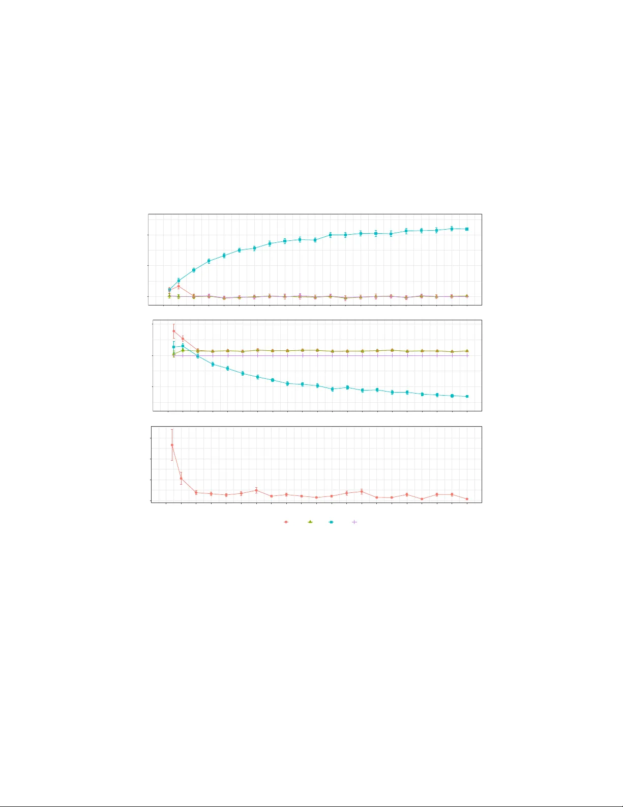
Estimating Causal P eer Inﬂuence in Homophilous So cial Net w orks b y Inferring Laten t Lo cations Edw ard McF o wland I II ∗ Cosma Rohilla Shalizi † Abstract So cial inﬂuence cannot be identiﬁed from purely observ ational data on so cial netw orks, b ecause suc h inﬂuence is generically confounded with laten t homophily , i.e., with a no de’s net work partners being informativ e ab out the no de’s attributes and therefore its b eha vior. If the netw ork gro ws according to either a laten t comm unity (stochastic blo c k) mo del, or a contin uous latent space model, then latent homophilous attributes can b e consistently estimated from the global pattern of so cial ties. W e sho w that, for common versions of those tw o netw ork mo dels, these esti- mates are so informativ e that con trolling for estimated attributes allows for asymptotically un biased and consistent estimation of so cial-inﬂuence eﬀects in linear models. In particular, the bias shrinks at a rate which di- rectly reﬂects ho w muc h information the netw ork provides about the latent attributes. These are the ﬁrst results on the consistent non-experimental estimation of so cial-inﬂuence eﬀects in the presence of latent homophily , and we discuss the prosp ects for generalizing them. 1 In tro duction: Separating Homophily from So- cial Inﬂuence It is an ancien t observ ation that p eople are inﬂuenced by others (nearb y) in their so cial netw ork—that is, the b eha vior of one node in a so cial net work adapts or resp onds to that of neigh b oring nodes. Such social inﬂuence is not just a curios- it y , but of deep theoretical and empirical imp ortance across the so cial sciences. It is also of great imp ortance to v arious kinds of social engineering, e.g., mar- k eting (esp ecially , but not only , “viral” marketing), public health (ov er-coming “p eer pressure” to engage in risky behaviors, or using it to spread healthy ones), education (“peer eﬀects” on learning), p olitics (“p eer eﬀects” on voting), etc. Con versely , it is an equally ancien t observ ation that p eople are not randomly assigned their so cial-net work neigh b ors. Rather, they sele ct them, and tend to select as neighbors those who are already similar to themselv es. (This is not ∗ Department of Information and Decision Sciences, Carlson School of Management, Uni- versit y of Minnesota † Statistics Departmen t, Carnegie Mellon Universit y , and the Santa F e Institute 1 necessarily b ecause they pr efer those who are similar; all more-desirable p oten- tial partners might ha ve already b een claimed or otherwise excluded [Martin, 2009].) This homophily means that netw ork neighbors are informative about laten t qualities a node p ossesses, providing an alternative route by which a no de’s b eha vior can b e predicted from their neighbors. Eﬀorts to separate ho- mophily from inﬂuence hav e a long history in studies of netw orks [Leenders, 1995]. Motiv ated b y the contro v ersy o ver Christakis and F owler [2007], Shalizi and Thomas [2011] show ed that unless al l of the no dal attributes which are relev ant to b oth social-tie formation and the b eha vior of interest are observed, then social-inﬂuence eﬀects are generally uniden tiﬁed. The essence of this result is that a so cial net work is a mac hine for cr e ating selection bias 1 . Shalizi and Thomas [2011, § 4.3] did hint at a p ossible approach for iden ti- ﬁcation of so cial inﬂuence, even in an homophilous netw ork. When a netw ork forms by homophily , a no de is likely to b e similar to its neighbors. F ollow- ing this logic, these neighbors are likely to b e similar to their neighbors and therefore the original node. In the simplest situations, where there are only a limited num b er of no de t yp es, this means that a homophilous net work should tend to exhibit clusters with a high within-cluster tie density and a low density of ties across clusters. Breaking the netw ork into suc h clusters might, then, pro- vide an observ able pro xy for the latent homophilous attributes. The same idea w ould work, mutatis mutandis , when those attributes are contin uous. Shalizi and Thomas [2011] therefore conjectured that, under certain assumptions on the netw ork-gro wth pro cess (which they did not specify), unconfounded causal inferences could be obtained by controlling for estimate d lo cations in a latent space. Subsequen tly , Davin et al. [2014] and W orrall [2014] show ed that, in lim- ited simulations, such controls can indeed reduce the bias in estimates of so cial inﬂuence, at least when the netw ork grows according to certain, particularly w ell-b eha ved, mo dels. In this pap er, w e complement these simulation studies by establishing suf- ﬁcien t conditions under which controlling for estimated latent lo cations leads to asymptotic al ly un biased and consistent estimates of so cial-inﬂuence eﬀects. Additionally , we sho w that for a particular class of netw ork mo dels, the remain- ing ﬁnite-sample bias shrinks exp onen tially in the size of the net work, while this bias shrinks polynomially for a more general class of netw ork models. T o the b est of our knowledge, our results provide the ﬁrst the or etic al guaran tees of consisten t estimation of so cial-inﬂuence eﬀects from non-exp erimen tal data, in the face of latent homophily . Additionally , we pro vide our own sim ulations to supp ort and explore our theoretical results. Section 2 lays out the basics of our setting, starting with assumptions ab out the pro cesses of netw ork formation and so cial inﬂuence (and the links b etw een them), and rehearsing relev ant results from the prior literature on latent com- m unity mo dels ( § 2.2) and contin uous latent space mo dels ( § 2.3). Section 3 presen ts our main results about the asymptotic estimation of social inﬂuence in the presence of latent homophily (proofs are deferred to § 6). Section 4 provides 1 A turn of phrase gratefully b orrow ed from Ben Hansen. 2 a set of sim ulations that conﬁrm our theoretical results and explore settings that div erge from ours. Section 5 discusses the strengths and limits of our results in the context of the related literature. 2 Setting and Assumptions The graphical causal m odel 2 capturing social inﬂuence in our setting is sho wn in Figure 1. More sp eciﬁcally , we are interested in the patterns of a certain b eha vior or outcome o ver time, across a social net work of n no des. The behavior of no de i ∈ { 1 , . . . , n } at time t ∈ { 1 , . . . , T } is observed and represented by random v ariable Y i,t ∈ R , for some given time-horizon T . So cial netw ork ties (or links) are also observed and represented through an n × n adjacency matrix A , with A ij = 1 if i receives a tie from j , and A ij = 0 otherwise. In many con texts these ties are undirected, so A ij = A j i , but generally our results do not require this. (In the latent communit y setting [ § 2.2], the pro cedure considered b y Gao et al. [2017] assumes an undirected netw ork, and therefore the results of ours which rely on that pro cedure also make this assumption.) As this notation suggests, w e assume that the netw ork of so cial ties do es not c hange, at least o ver the time-scale of the observ ations 3 . In addition to the observ ed b eha viors and ties of no de i , w e assume there exist a d -dimensional latent vector C i whic h controls its lo cation in the net- w ork; we deﬁne C as the arra y [ C 1 , C 2 , . . . , C n ]. F urthermore, we assume that Pr ( A ij = 1 | C ) = w ( C i , C j ) for some measurable function w , and that the ran- dom v ariables A ij and A lm are conditionally indep enden t given C , ∀ i, j 6 = l , m . The time-inv ariant vector X i represen ts the set of all other (i.e., netw ork irrel- ev ant) attributes for no de i , which eﬀect Y i,t but not A ij . The linear structural-equation mo del that explains the b eha vior of no de i at time t is thus Y i,t +1 = α 0 + α 1 Y i,t + β P j ( Y j,t A ij ) P j A ij + γ T 1 C i + γ T 2 X i +  i,t +1 , (1) where γ 1 and γ 2 serv e as appropriately-sized vectors of co eﬃcients. Under the assumptions of linearly-indep enden t regressors and strict exogeneit y—i.e., E [  i,t +1 | Y i,t , A ij , C i , X i ] = 0 ∀ i, j, t —our goal is to identify , and estimate, β , the co eﬃcien t for so cial inﬂuence. Given that we neither observe X i nor C i , we cannot estimate the regression co eﬃcien ts in a mo del of the form presen ted in 2 W e do not mean to take sides in the dispute b etw een the partisans of graphical causal models and those of the p oten tial-outcomes formalism. The expressiv e p o wer of the latter is strictly weak er than that of suitably-augmented graphical mo dels [Richardson and Robins, 2013], but we could write everything here in terms of potential outcomes, alb eit at some cost in space and notation. 3 Latent space mo deling of dynamic netw orks is still in its infancy . F or some preliminary eﬀorts, see, e.g., DuBois et al. [2013], Ghasemian et al. [2015] for block models, and Sark ar and Mo ore [2006] for contin uous-space models. 3 C(i) A(i,j) A(i,l) Y(i,t-1) Y(i,t) Y(i,t+1) C(j) A(j,l) Y(j,t-1) Y(j,t) C(l) Y(l,t-1) Y(l,t) X(i) X(j) X(l) Figure 1: The graphical causal mo del for our setting. Boxes indicate observ- ables, and circles latent v ariables; solid lines indicate causal relations betw een observ ables (either autoregressiv e or p eer-inﬂuence), while dotted lines indicate the inﬂuence of latent homophilous v ariables, and dashed lines indicate the in- ﬂuence of other cov ariates. F or simplicity , we omit Y ( j, t + 1) and Y ( l , t + 1), as well as their asso ciated arrows. 4 (1). How ev er, we c an estimate the coeﬃcients of the follo wing mo del: Y i,t +1 = α 0 + α 1 Y i,t + β P j ( Y j,t A ij ) P j A ij + γ T 0 ˆ C i + η i,t +1 , (2) where ˆ C i is an estimated or disco vered location for no de i and the noise term η i,t +1 can b e deﬁned as η i,t +1 =  i,t +1 + γ T 2 X i +  γ T 1 C i − γ T 0 ˆ C i  . Our general setting is therefore deﬁned by an additional assumption: X i | = Y j,t | ˆ C i . (3) The assumptions of indep endence must b e justiﬁed on substan tive grounds, in the sp eciﬁc context of the study where so cial inﬂuence is b eing estimated. 2.1 Discussion on the General Setting W e ﬁnd it b eneﬁcial to pro vide intuition on ho w v arious facets of our setting enable the iden tiﬁcation of so cial-inﬂuence eﬀects. W e b egin b y recognizing that the relativ ely permanent attributes of no de i can b e divided in t wo cross-cutting w ays. On the one hand, some attributes are (in a giv en study) observ able or manifest, and others are latent. On the other hand, a given attribute could be a cause of the b eha vior of interest Y i,t , or a cause of net work ties ( A ij ), or of b oth. (Attributes which are irrelev ant to b oth b eha vior and netw ork ties are ignored here as they hav e no b earing on our ultimate goal). One of the key assumptions embedded in our tie formation pro cess (i.e., Pr ( A ij = 1 | C ) = w ( C i , C j )) is that al l of the netw ork-relev an t attributes of no de i can b e represented b y a single vector-v alued latent v ariable C i , whether or not they are also relev ant to the b eha vior of interest. There may b e attributes that are incorp orated into C i whic h are relev an t only to net work ties, not b ehavior, and indep endent of the other attributes; these are of no concern to us, and can b e regarded as part of the noise in the tie-formation pro cess. Net work mo dels that satisfy this assumption—i.e., that all ties are conditionally indep enden t of each other giv en the laten t v ariables for each node—are sometimes called “graphons” or “ w -random graphs” and are clearly exc hangeable (p erm utation-inv ariant) o ver no des. Conv ersely , the Aldous-Hoov er theorem [Kallen b erg, 2005, ch. 7] sho ws that this condition is, in fact, the generic form of exc hangeable random net works. Our subsequent assumption, sp eaking roughly , is that by observing the whole netw ork A ij (whic h inheren tly includes the information it con tains with resp ect to the laten t array C ), Y i,t pro vides no additional information (in the limit) for no de i ’s laten t lo cation C i . W e also recognize that as a result of the assumptions of linear-dep endence and strict exogeneity in (1), if all the v ariables relev ant to tie-formation and node b eha vior are observed, the ordinary least squares (OLS) estimator provides an 5 un biased estimate ( ˆ β OLS ) of β . How ever, since C i and X i are b oth unobserved, and therefore their eﬀects are contained in the η i,t +1 of (2), ˆ β OLS will generally con tain omitted v ariable bias if either of these latent v ariables are correlated with Y j,t , conditional on the observ ed regressors. Intuitiv ely , the latent nature of X i will not produce bias b ecause (3) implies that given estimated locations, nothing can b e learned ab out a node’s unobserv ed, netw ork-irrelev ant attributes b y observing a neighbor’s b eha vior (or vice-v ersa). Mathematically , this means that the contribution of γ T 2 X i to η i,t +1 is uncorrelated with Y j,t , given the estimated locations, and therefore this term do es not bias the estimates of β ; instead it just increases the v ariance of the noise term. It is also not necessary that E [ η i,t +1 ] = 0; if it has a non-zero v alue, it would then b e incorp orated into the estimate of the intercept ( α 0 ), and therefore not induce bias in β . W e hav e therefore to only consider the other contribution to η i,t +1 , ( γ 1 C i − γ 0 ˆ C i ), and whether it is correlated with Y j,t giv en ˆ C i and Y i,t . k C i − ˆ C i k is the error in estimating the true lo cation, whic h manifests as measuremen t error in OLS estimation of β in (2). Given that Y j,t is a causal descendan t of C j , and C j is p ositiv ely correlated with C i if A ij = 1 (from homophily), this measurement error induces bias in the estimate of β . Intuitiv ely (and formally sho wn in Lemma 1 b elo w) if ˆ C = C (i.e., there is no measuremen t error) the OLS estimate of β in (2) will b e un biased and consistent; although, this estimate will likely ha ve a larger v ariance than would the OLS estimate of β from (1), given that the former estimate do es not con trol for X i . It should further be plausible (and is formally sho wn in § 3 b elow) that if ˆ C is a “goo d enough” estimate of C —i.e., one which is consistent and conv erges suﬃcien tly rapidly—the cov ariance b et ween η i,t +1 and Y j,t shrinks fast enough that the OLS estimate from (2) will still yield asymptotically unbiased and consistent estimates of β . Essentially , the OLS estimator for β in (2) trades-oﬀ the bias (exp erienced by the OLS estimator for β in (1)) from omitting the laten t location v ariable C i , with the bias from measuring (estimating) the lo cation imprecisely with ˆ C i . How ev er, the abilit y to obtain a “go o d enough” estimate of C will mak e this trade-oﬀ w orthwhile; if the measurement error con verges to zero, then the bias it induces should also con verge to zero, while the omitted v ariable bias p ersists. There do es not (yet) exist results providing suc h “go o d enough” estimates of latent no de lo cations ˆ C for arbitrary graphons. F or this reason, our re- sults sp ecialize to t wo settings, where the latent no de lo cations C and the link-probabilit y function w tak e particularly tractable forms: laten t commu- nit y (stochastic blo c k) mo dels and the more general (contin uous) latent space mo dels. Both mo del t yp es ha ve b een extensively explored in the literature. It is by building on results for these mo dels that we can ﬁnd regimes where the so cial-inﬂuence co eﬃcien ts can b e estimated consistently . It is, how ever, w orth noting that for any graphon mo del where “go od enough” estimates of laten t no de lo cations ˆ C exist, an analog to our results for laten t space mo dels (Theorem 2) can b e built. 6 2.2 The Latent Communities Setting In our ﬁrst setting, we presume that no des split into a ﬁnite num b er of discrete t yp es or classes ( k ), which in this context are called blo c ks , mo dules or com- m unities . More precisely , there exists a function σ : { 1 , . . . , n } 7→ { 1 , . . . , k } assigning no des to communities. W e sp eciﬁcally assume that the net work is generated by a sto c hastic block mo del , which is to say that there are k com- m unities 4 , that σ ( i ) iid ∼ ρ , for some ﬁxed (but unkno wn) m ultinomial distribution ρ , and that w is given by a k × k aﬃnity matrix , so that Pr ( A ij = 1 | σ ( i ) = a, σ ( j ) = b ) = w ab . W e ma y translate betw een σ (a sequence of categorical v ariables) and our earlier C (an n × d matrix of no de lo cations) b y the usual device of in tro ducing indicator or “dummy” v ariables for k − 1 of the communities, so that C i is a k − 1 binary v ector (i.e., d = k − 1) which is a function of σ ( i ) and vice v ersa. Each p ossible v alue of C i is either the origin, or a corner of the simplex; this basic observ ation will b e imp ortant b elo w. The ob jectiv e of communit y detection or communit y disco very is to provide an accurate estimate ˆ σ or ˆ C from the observed adjacency matrix A , i.e., to say whic h communit y each no de comes from, sub ject to a p ermutation of the lab el set. (“Accuracy” here is often measured as the prop ortion of mis-classiﬁcation.) Since the problem was p osed by Girv an and Newman [2002] a v ast literature has emerged on the topic, spanning many ﬁelds, including physics, computer science, and statistics; see F ortunato [2010] for a review. How ever, we may summarize the most relev an t ﬁndings as follo ws. 1. F or net works which are generated from latent communit y mo dels, under v ery mild regularity conditions, it is p ossible to recov er the comm unities consisten tly , i.e., as n → ∞ , Pr  ˆ C 6 = C  → 0 [Bick el and Chen, 2009, Zhao et al., 2012]. That is, with probability tending to one, al l of the comm unity assignments are correct, up to a global p erm utation of the lab els b et ween C and ˆ C . 2. Such consistent comm unity discov ery can be achiev ed b y algorithms whose running time is p olynomial in n . 3. The minimax rate of con vergence is in fact exp onen tial in n (and can be ac hieved by the algorithms mentioned b elo w). These p oin ts, particularly the last, will b e imp ortan t in our argument b elo w, and so we now elab orate on them. Recen tly , Zhang and Zhou [2016] prov ed that under v ery mild regularity conditions the minimax rate of con vergence for undirected net works generated 4 Some of the theory we rely on b elow allows the number of communities to grow with the size of the network, though with at a rate p osited to b e known a priori , and not to o fast. W e leav e dealing with this complication to future work. 7 from laten t communit y mo dels is in fact exp onen tial in n . F urthermore, Gao et al. [2017] exploits techniques provided by Zhang and Zhou [2016] to prop ose an algorithm p olynomial in n that ac hieves this minimax rate, under slightly mo diﬁed but equally mild regularit y conditions. More precisely , Gao et al. [2017] considers a general undirected sto c hastic block mo del, parametrized b y n , the num b er of no des; k , the num b er of communities; a and α ≥ 1, where a n = min i w ( i, i ) ≤ max i w ( i, i ) ≤ αa n , ensuring that within-communit y edges are “suﬃciently” dense; b , where bα n ≤ 1 k ( k − 1) P i 6 = j w ( i, j ) ≤ max i 6 = j w ( i, j ) b n , with 0 < b n < a n < 1, ensuring that betw een-communit y edges are “suf- ﬁcien tly” sparse; and β ≥ 1, where the num b er of no des in comm unity k , n k ∈ h n β k , β n k i , ensuring that comm unity sizes are “suﬃciently” comparable. Zhang and Zhou [2016] and Gao et al. [2017] diverge sligh tly as the former only requires max i 6 = j w ( i, j ) ≤ b n and a n ≤ min i w ( i, i ). Additionally , the latter sligh tly restricts the parameter space b y requiring the k th singular v alue of the aﬃnit y matrix w to b e greater than some parameter λ . The general context of the theory describ ed in Zhang and Zhou [2016], Gao et al. [2017] is deﬁned for absolute constant β ≥ 1 and also in Gao et al. [2017] for absolute constant α ≥ 1, while k , a , b , and λ are functions of n and therefore v ary as n grows. Ho wev er, in our context, the netw ork do es not change (ov er the time-scale of in terest); therefore, we only consider latent comm unities where k , a n , b n , and λ are also absolute constants. W e shall refer to this whole set of restrictions on the latent communit y mo del as “the GMZZ conditions”. F or a laten t comm unity mo del satisfying the GMZZ conditions, the minimax rate of conv ergence for the expected pr op ortion of errors is exp  − (1 + o (1)) nI 2  , k = 2 (4) exp  − (1 + o (1)) nI β k  , k ≥ 3 , (5) where I is the R´ en yi [1961] divergence of order 1 2 b et w een tw o Bernoulli distri- butions with success probabilities  a n  and  b n  : D 1 2  Ber  a n  k Ber  b n  . Recall that β in addition to k , a n , b n are, in our context, constant in n ; therefore, (4) and (5) both reduce to exp ( − O ( n )). The algorithm of Gao et al. [2017] ac hieves this rate at a computational cost p olynomial in n . More sp eciﬁcally , the time complexit y of the algorithm is (by our calculations) at most O ( n 3 ), but w e do not know whether this is tight. It would b e v aluable (but b eyond the scop e of this w ork) to kno w whether this rate is also a lo w er b ound on the computational cost of obtaining minimax error rates, and if the complexity could b e reduced in practice for very large graphs via parallelization. W e close this section by introducing a bit of notation (which will simplify some later statements) and making a claim (which will b e supp orted later). W e will write δ ( n ) for the error probabilit y , i.e., the probabilit y that ˆ C i 6 = C i for at least one i ∈ 1 : n . The claim is that even though the results of Zhang and Zhou [2016] and Gao et al. [2017] concern the prop ortion of mis-classiﬁed no des, they 8 actually constrain the probability of making an y mis-classiﬁcations at all, and imply δ ( n ) = e − O ( n ) (Lemma 3). 2.3 The Contin uous Laten t Space Setting The second setting w e consider is that of con tinuous laten t space models. In this setting, the laten t v ariable on eac h no de, C i , is a p oin t in a con tinuous metric space (often but not alwa ys R d with the Euclidean metric), and w ( C i , C j ) is a decreasing function of the distance betw een C i and C j , e.g., a logistic function of the distance. This link-probability function is often taken to b e known a priori . The latent lo cations C i iid ∼ F , where F is a ﬁxed but unknown distribution, or, more rarely , a p oin t pro cess. Diﬀeren t distributions ov er netw orks thus corresp ond to diﬀeren t distributions o ver the contin uous laten t space, and vice v ersa. P arametric versions of this model ha ve b een extensiv ely developed since Hoﬀ et al. [2002], esp ecially in Bay esian contexts. Less attention has b een paid to the consistent estimation of the latent lo cations in such mo dels, than to the estimation of communit y assignments in latent communit y mo dels. Recent results by Asta [2015, c h. 3], how ever, sho w that when w is a smo oth function of the metric whose logit transformation is b ounded, the maxim um likelihoo d estimate ˆ C con verges to C . Moreo ver, the probabilit y of an error of size  or larger is O (exp  − κn 2  ), where the constan t κ dep ends on the purely geometric prop erties of the space (see § 3.2 b elow). This result holds across distributions of the C i , but may not b e the b est p ossible rate. 3 Con trol of Confounding Giv en the (assumed) true structural equation in (1), our ultimate goal is to pro vide b oth an estimator of β , and the corresp onding suﬃcien t conditions under whic h that estimator will hav e desirable statistical prop erties. Recall that these prop erties of the estimator are ev aluated in the presence of estimated or disco vered no de lo cations ˆ C , rather than the true locations C . Going forw ard, therefore, unless otherwise noted, our estimator of interest is OLS for β in (2). Finally , all pro ofs of the results stated b elow are provided in § 6. W e b egin b y establishing this estimator’s prop erties in a baseline case: when the estimates of no de locations are perfect, Pr  C 6 = ˆ C  = 0. Lemma 1. Under the assumptions fr om Se ction 2, if Pr  C 6 = ˆ C  = 0 , then the or dinary le ast squar es estimate of β in (2) is unbiase d and c onsistent. Giv en that we establish that OLS estimator will exhibit unbiasedness and consistency , when no de lo cations can b e p erfectly inferred, let us now consider its properties when the node lo cation are inferred with error. The cov ariance of in terest is that b et ween P j ( Y j,t A ij ) P j A ij and the contribution to the error—i.e., 9 η i,t +1 in (2)—arising from using the estimated rather than the real communities. W e hav e seen ( § 2.1), that in our setting, under assumption (3), this term is just γ T 1 C i − γ T 0 ˆ C i . Moreov er, w e will only need to consider that cov ariance conditional on ˆ C i and ˆ C j , and the other regressor in (2), i.e., Y i,t . Lemma 2. Supp ose that the assumptions fr om Se ct ion 2 hold. Then Co v " P j ( Y j,t A ij ) P j A ij , ( γ T 1 C i − γ T 0 ˆ C i )      A, Y i,t # (6) = P j A ij γ T 1  Co v [ C i , C j | A ] + ξ ij V ar [ C i | A ] + P l 6 = i,j ζ ij l Co v [ C i , C l | A ]  γ 1 P j A ij , wher e by Cov [ C i , C j ] we me an the d × d matrix of c o or dinate-wise c ovarianc es, and similarly for V ar [ C i ] , and the ξ s and ζ s ar e c onstants c alculable in terms of the mo del c o eﬃcients and the adjac ency matrix (and ar e made explicit in the pr o of of the lemma). Lemma (2) establishes an imp ortan t relationship b et ween the bias exp eri- enced b y the OLS estimator and the degree of homophily in the net work. Recall that we observe a net work (represen ted by A ) whose ties are formed under ho- mophily , based on (unobserved) no de lo cations. F urthermore, it is precisely the fact that this netw ork is observ ed (and conditioned on) that opens the confound- ing bac kdo or pathw ay in the causal graph (Figure 1). F or clarit y , the net work is conditioned on b ecause it enables the true structural equation (1) to select if the b eha vior of no de i is regressed on the b ehaviors of no des j . Moreov er, when homophily has a large impact on tie formation, the v alue Cov [ C i , C j ] will b e large, as node i will ha ve more connections from closer no des j (i.e., roughly , C i ≈ C j ). W e then recognize that although observing the netw ork A (and failing to observe the latent locations C ) op ens the homophilous confounding pathw ay , the netw ork also manifests this homophily in the ties that are formed, which can b e used to form estimates of the laten t lo cations ˆ C . F urther, condition- ing on A implies conditioning on ˆ C i and ˆ C j , as they are deterministic (albeit complicated) functions of A . F rom Lemma (2) w e then see that the bias in our estimate ˆ β OLS is prop ortional to the amoun t of cov ariance b et ween the true laten t lo cations of nodes that share a tie, b ey ond that which is accoun ted for b y their lo cation estimates. Therefore, when this conditional cov ariance is zero, ˆ β OLS is unbiased and consistent. There are tw o individually suﬃcien t (but not necessary) conditions for (6) to b e zero: 1. C i | = C j | ˆ C i , ˆ C j , i.e., C i and C j are indep enden t given their estimates, 2. C i = ˆ C i and C j = ˆ C j , i.e., C i and C j are equal to their estimates. The second condition will generally not b e true at an y ﬁnite n . The ﬁrst con- dition is also very strong; it implies that ˆ C is (roughly sp eaking) a suﬃcien t 10 statistic for C . This suﬃciency property implies that ev en in learning C i (the true location of node i ) we obtain no additional information about C j (the lo- cation of any other no de j ) not already captured in ˆ C . W e are not aw are of any estimates of latent node lo cations in netw ork mo dels which hav e such a suﬃ- ciency prop ert y , and w e strongly susp ect this is because they generally are not suﬃcien t. (T o get a sense of what would b e entailed, supp ose that A ij = 1, and w e knew we were dealing with a homophilous latent comm unity mo del. Then ˆ C would hav e to b e so informative that ev en if an Oracle told us C i , our p oste- rior distribution ov er C j w ould b e unchanged.) W e may , how ever, make further progress in the tw o sp eciﬁc settings of latent communities and of contin uous laten t spaces. 3.1 Con trol of Confounding with Laten t Comm unities Let us ﬁrst consider the setting where the net work formation is that of a ho- mophilous laten t communit y pro cess, whic h follows the conditions laid out in § 2.2. In suc h a setting, we can make additional statements with resp ect to the Co v h C i , C j    ˆ C i , ˆ C j i , and subsequently the bias exp erienced by the OLS estima- tor. More sp eciﬁcally , these statements are made assuming a deterministic and minimax algorithm—one that ac hieves the minimax rate of con vergence for the exp ected prop ortion of no de location errors —is utilized to estimate ˆ C as in Gao et al. [2017]. Lemma 3. Supp ose that the assumptions fr om Se ction 2 hold, the network forms ac c or ding to a latent c ommunity mo del, satisfying the GMZZ c onditions, and ˆ C is estimate d using a minimax algorithm. Then Pr n X i 1 { ˆ C i 6 = C i } ≥ 1 ! ≤ e − O ( n ) . W e therefore hav e that the probabilit y of making any error in the estimation of latent no de lo cations con verges (exp onen tially) to zero in n . This result from Lemma 3 will play a critical role in pro ving the next result: Lemma 4. Supp ose that the assumptions fr om Se ction 2 hold, the network forms ac c or ding to a latent c ommunity mo del, and ˆ C is estimate d by a deter- ministic algorithm with err or r ate δ ( n ) . Then Co v [ C i , C j | A ] = O ( δ ( n )) . If, in addition, the latent c ommunity mo del satisﬁes the GMZZ e quations, and ˆ C is estimate d using a minimax algorithm, then Co v [ C i , C j | A ] = O  e − O ( n )  . The ability to not only show the conv ergence of Co v [ C i , C j | A ], but also its rate of decay for ﬁnite- n leads to a n umber of imp ortan t conclusions. 11 Theorem 1. Supp ose that the assumptions fr om Se ction 2 hold, the network forms ac c or ding to a latent c ommunity mo del, and ˆ C is estimate d with err or r ate δ ( n ) . Then the or dinary le ast squar es estimate for β in (2) is asymptotic al ly unbiase d and c onsistent, and the pr e-asymptotic bias is O ( δ ( n )) . If, in addition, the latent c ommunity mo del satisﬁes the GMZZ c onditions and ˆ C is estimate d using a deterministic and minimax algorithm, then the pr e-asymptotic bias is exp onential ly smal l in n . W e susp ect that it is also p ossible to provide a precise expression of a de- terministic ﬁnite- n b ound on the bias—likely as the solution to an optimization problem inv olving (unknown) parameters of the structural equation (1)—but lea ve this as a useful topic for future inv estigation. Note: W e hav e stated Lemma 4 and Theorem 1 (and the subsidiary Lemma 5) in tw o parts to clarify that most of their logic will apply whenever some deterministic algorithm is capable of communit y disco very with a v anishing error rate δ ( n ). The GMZZ conditions are inv oked as regularity conditions under whic h δ ( n ) can be made exp onen tially small at only a polynomial computational cost. If the GMZZ conditions are implausible for a particular application, but some other algorithm can, in that situation, deliver δ ( n ) → 0, then it can be used instead within the scop e of our analysis. 3.2 Con trol of Confounding with Contin uous Laten t Space W e now turn our atten tion to setting where the netw ork follows a homophilous con tinuous latent space mo del. Recall that our treatment of the laten t c ommu- nity setting relies on the fact that Pr  ˆ C 6 = C  → 0, i.e., with probability tend- ing to one the estimated comm unities match the actual comm unities exactly . Imp ortan tly , this is not known to happ en for contin uous latent space models, and seems v ery implausible for estimates of contin uous quantities, how ever we still can make progress. As men tioned in § 2.3, Asta [2015, ch. 3] has sho wn that if the link-probabilit y function is kno wn and has certain natural regularity prop erties (detailed b elo w), then the probability that the sum of the distances b etw een true locations and their maximum likelihoo d estimates exceeds  go es to zero exp onentiall y in n 2 (at least). More sp eciﬁcally , the result requires the link-probability function to b e smo oth in the underlying metric and bounded on the logit scale, and requires the laten t space’s group of isometries 5 to ha ve a b ounded num b er of connected comp onen ts. (This is true for Euclidean spaces of an y ﬁnite dimension, where the num b er of connected comp onen ts is alwa ys 2.) If these ab o ve conditions are met—whic h we shall refer to as “the Asta conditions”—then Pr n X i =1 d ( ˆ C i , C i ) ≥  ! ≤ N ( n,  ) e − κn 2  5 An isometry is a transformation of a metric space whic h preserves distances b etw een points. These transformations naturally form groups, and the prop erties of these groups control, or enco de, the geometry of the metric space [Brannan et al., 1999]. 12 where the N is a kno wn function, polynomial in n and in 1 / , depending only on the isometry group of the metric, and κ is a kno wn constant, calculable from the isometry group and the b ound on the logit. Since the maximum of n distances is at most the sum of those distances, this further implies that Pr  max i ∈ 1: n d ( ˆ C i , C i ) ≥  )  ≤ N ( n,  ) e − κn 2  . (7) With this, we can make the follo wing asymptotic result. Theorem 2. Supp ose that the assumptions fr om Se ction 2 hold, the network forms ac c or ding to a c ontinuous latent sp ac e mo del satisfying the Asta c ondi- tions, that the no de-lo c ation distribution F has c omp act supp ort, and that ˆ C is estimate d by maximum likeliho o d. Then the or dinary le ast squar es estimate for β in (2) is asymptotic al ly unbiase d and c onsistent, and the pr e-asymptotic bias is p olynomial ly smal l in n . The Asta conditions do not require F to hav e compact supp ort, but we use this assumption for mathematical conv enience in our deriv ation of the b ound on the bias. The assumption do es, strictly sp eaking, rule out using a Gaussian distribution for the laten t lo cations. It is, how ever, compatible with using a Gaussian that is truncated to 0 beyond some (large) distance from the origin. W e susp ect the compact-supp ort assumption can b e weak ened to merely as- suming that F is tigh t, or that it has suﬃcien tly light tails, but leav e this to future work. W e susp ect that it is also p ossible to provide a precise expression of a deterministic ﬁnite- n b ound on the bias—though likely not the solution to optimization problem, as we susp ect for latent communit y mo dels—and leav e this to o as a useful topic for future inv estigation. 4 Sim ulations In observ ational studies o ver social net works, consisten t estimation of the social- inﬂuence parameter requires the ability to disen tangle its eﬀe ct from that of homophily . Ab ov e, we gav e conditions under whic h consistent (and asymptot- ic al ly unbiased) estimates of social inﬂuence is p ossible. The sim ulations here aim to pro vide an empirical complement to these theoretical results, verifying that our approach do es in fact provide consisten t estimates of p eer-inﬂuence, and ac hieves relatively small amounts of bias even at manageable sample sizes. Additionally , w e explore ho w estimates of the p eer-inﬂuence parameter b eha v e as w e (smo othly) depart from the conditions of our theory , conﬁrming that the results are robust to at least some violations of the assumptions. Finally , the ev aluation of our approach in these simulations are done in the context of other estimation approaches, for prop er comparisons. 4.1 Sim ulation Setup Giv en that Davin et al. [2014] has already conducted an empirical sim ulation study in the context of latent space models, we will consider the latent com- 13 m unity model setting to in vestigate our theoretical results via sim ulation. W e use the follo wing R [R Core T eam, 2020] pac k ages to build our simulated net- w ork mo dels: her gm [Sch w einberger and Luna, 2018], mler gm [Stewart and Sc hw einberger, 2018], and igr aph [Csardi and Nepusz, 2006]. In our sim ula- tion setting, we ha ve three net work parameters of in terest: n , or the n umber of no des in the net work; p within , or the probability of an edge b et w een no des in the same comm unities; p between , or the probabilit y of an edge b et ween no des in diﬀerent communities. F or our simulations, we sp eciﬁcally consider n ∈ { 20 , 25 , 50 , 100 , . . . , 1000 } and b oth p within , p between ∈ { 0 . 1 , 0 . 15 , 0 . 2 , . . . , 0 . 9 } . Instead of considering all combinations of parameter v alues, we select a v alue of eac h parameter as a reference point ( n = 500, p within = 0 . 75, p between = 0 . 25), measuring ho w estimator prop erties of interest (e.g., bias) c hange for one pa- rameter, while keeping the others ﬁxed. W e tak e the num b er of blo c ks and the probabilit y of communit y membership to b e ﬁxed at k = 4 and 1 k , resp ec- tiv ely . (As suggested by our theory , w e ﬁnd that the results of our approach are consisten t for any ﬁxed num b er of blocks, of comparable sizes.) Therefore, the laten t communit y netw ork (i.e., adjacency matrix A ∈ [0 , 1] n × n and communit y mem b ership σ ∈ [ k ] n ) for eac h sim ulation is dra wn from the mo del space param- eterized as Θ ( n, k , a, b, β ), which satisﬁes the conditions describ ed in Gao et al. [2017] 6 . More sp eciﬁcally , in our sim ulations, a ≈ n · p within , b ≈ n · p between , k = 4, and E [ β ] = 1. Giv en our net work class and parameter set, w e now deﬁne the data gener- ation process of interest that will describ e the b ehavior of no de level v ariables across the netw ork. W e again consider the causal mo del deﬁned in Figure 1, and the subsequent linear structural-equation mo del deﬁned in (1), which we restate for clarity: Y i,t +1 = α 0 + α 1 Y i,t + β P j ( Y j,t A ij ) P j A ij + γ T 1 C i + γ T 2 X i +  i,t +1 . In eac h simulation, using Sofrygin et al. [2017], w e generate structural equa- tions with parameters following a normal distribution N ( µ, σ 2 ): α 0 ∼ N (1 , 1), α 1 ∼ N (10 , 1), β ∼ N (0 . 1 , 1), γ 1 ∼ N (10 , 1) and γ 2 ∼ N (1 , 1). Note that C i ∈ { 1 , . . . , k } starts as an integer (comm unit y identiﬁcation) label, but for the purp ose of the regression is translated into a k − 1 binary vector, and therefore, γ 1 is also appropriately translated into a k − 1 vector. Additionally , we generate the following no de-level v ariables:  i,t +1 ∼ N (0 , 10) and X i ∼ N (0 , 1), the lat- ter whic h w e treat as a single v ariable capturing un-c hanging, netw ork-irrelev ant attributes for eac h node. Finally , our goal is to estimate β , the co eﬃcien t for so cial inﬂuence. When the abov e is the structural-equation mo del generating our data, OLS will provide an unbiased and consistent estimate of β , assuming we can observ e 6 The GMZZ conditions also include a parameter to control the diﬀerences across comm uni- ties of the within- and between-comm unity connection probabilities. W e omit this parameter as the within- and betw een-communit y connection probabilities are both constant across com- munities in our simulations. This restricted parameter space is discussed in Gao et al. [2017] as Θ 0 . 14 eac h of the v ariables relev ant to the netw ork (i.e., A ij and C i ) as w ell as those that are irrelev ant to the netw ork but still relev ant to b eha vior ( Y i,t , Y j,t , and X i ). How ever, in practice, we do not observe either C i or X i , and therefore consider the OLS estimator of β in (1) to b e our “Oracle” estimator. Moreov er, in practice, w e can obtain the OLS estimation of β in (2), whic h again w e restate for clarity: Y i,t +1 = α 0 + α 1 Y i,t + β P j ( Y j,t A ij ) P j A ij + γ T 0 ˆ C i + η i,t +1 , where ˆ C i is an estimated lo cation for no de i and the noise term η i,t +1 is now η i,t +1 =  i,t +1 + γ T 2 X i + ( γ T 1 C i − γ T 0 ˆ C i ) . It is the OLS estimator of β in this equation that our prop osed theory (in conjunction with algorithms for deriving ˆ C i ) pro vides suﬃcien t conditions for consistency and asymptotically unbiasedness; therefore w e consider this to b e our “Algorithm” estimator. Critically , the bias present in this estimator is induced by measurement error, resulting from the use of ˆ C i in place of the (unobserv ed) correct C i ; therefore we also estimate Y i,t +1 = α 0 + α 1 Y i,t + β P j ( Y j,t A ij ) P j A ij + γ T 1 C i + e i,t +1 , and consider this our “Correct” estimator. Note that this estimator is the limit of our consisten t Algorithm estimator; additionally , unlik e the Oracle estimator, it is unable to condition on the (unobserved) X i . Finally , w e also consider the OLS estimator of β in Y i,t +1 = α 0 + α 1 Y i,t + β P j ( Y j,t A ij ) P j A ij + u i,t +1 , whic h will hav e omitted v ariable bias because it incorrectly ignores the impact of homophily all together; therefore, w e consider this our “Incorrect” estimator. Our primary goal in the simulations is to observe changes in the bias exp e- rienced b y each estimator (i.e., Oracle, Algorithm, Correct, and Incorrect) de- scrib ed ab o ve, as conditions change. Additionally , we are also in terested in the relativ e v ariation of the estimators (as this has direct implications for conﬁdence in terv als and co verage probabilities), and again ho w this v ariation changes as conditions c hange. Finally , given that our Algorithm estimator trades bias from omitted v ariables for that from measurement error, fundamentally its eﬃcacy will be related to its degree of (estimation) error in node lo cations; therefore, w e also are interested in observing ho w this estimation error changes as conditions c hange. 4.2 Sim ulation Results In Figure 2, we observ e how v arious outcomes of interest v ary as the sample size (n umber of no des) increases (while the latent comm unit y mo del parameters 15 0 1 2 0 50 100 150 200 250 300 350 400 450 500 550 600 650 700 750 800 850 900 950 1000 Number of Nodes Bias in Coefficient −0.1 0.0 0.1 0 50 100 150 200 250 300 350 400 450 500 550 600 650 700 750 800 850 900 950 1000 Number of Nodes Standard Error Relative to Oracle 0.0 0.2 0.4 0.6 0 50 100 150 200 250 300 350 400 450 500 550 600 650 700 750 800 850 900 950 1000 Number of Nodes Community Missclassification Rate Estimator Algorithm Correct Incorrect Oracle Figure 2: Comparison of the exp ected prop erties of the estimators where ex- p ectations is computed ov er 50 random samples, allowing also for the forma- tion of 95% conﬁdence interv als. The parameter of interest is sample size n , which v aries, while the laten t communit y mo del parameters remain ﬁxed ( k = 4 , p within = 0 . 75 , p between = 0 . 25). 16 remain ﬁxed at their reference v alues). W e note that this simulation complies with our assumed setting and therefore our predictions (based on our theoretical results) of eac h estimator’s b eha vior should b e consisten t with what we observ e. Let us b egin by considering the ﬁrst tw o plots, whic h sho w each estimator’s bias (top)—i.e., E h ˆ β − β i —and exp ected standard error relative to that of the Oracle estimator (middle)— E h ˆ σ ˆ β − ˆ σ ˆ β Or acle i — as a function of sample size. These plots conﬁrm that the Oracle and Correct estimators are unbiased at all sample sizes, but the Correct estimator has larger v ariance, b ecause it do es not observ e X i . Additionally , the plots conﬁrm that ignoring the latent communit y (as in the Incorrect estimator) leads to (omitted v ariable) bias at all sample sizes, whic h in our simulation amounts to a bias exceeding 2 numerical units for β in the limit. (Since the exp ected true v alue of β across simulations, E [ β ] = 0 . 1, a bias of 2 units is a relative error of a remark able 2 , 000%.) Beyond this extreme bias, the estimator, additionally , b ecomes ov erconﬁdent in its (biased) estimation, which will lead to inaccurate conﬁdence interv als and p oor cov erage probabilit y . Finally , the plots conﬁrm that the Algorithm estimator (based on estimated node lo cations) con verges to the Correct estimator, and ac hieves consisten t and (asymptotically) un biased estimation of p eer-inﬂuence. Figure 2 also provides additional insight in the prop erties of the Algorithm estimator, in comparing it to the other estimators. Imp ortan tly , we observ e that even at mo derate sample sizes ( n = 100) the estimator app ears to reach its asymptotic b ehavior (e.g., unbiasedness). Moreov er, prior to reaching this asymptotic behavior, the Algorithm and Incorrect estimators ha ve similar levels of bias, while the Algorithm estimator has larger v ariance. This implies that the biases resulting from omitting the no de lo cations and using estimated lo cations (i.e. measuremen t error) are comparable, while the measuremen t error induces larger v ariance; therefore, at small sample sizes, the Incorrect estimator appears to provide a b etter estimation risk (with resp ect to loss in mean squared error). Ho wev er, as sample size increases, the trade-oﬀ b et ween these t wo sources of bias (and v ariance) b egins to increasingly fa vor the measurement error, and the Algorithm estimator provides b etter estimation risk. W e can see from the b ottom plot in Figure 2 that the risk of the Algorithm estimator is, as expected, a function of the ov erall error in the node lo cations. Additionally , this estimator reac hes its asymptotic behavior relatively quic kly giv en the exp onen tial decay in the measurement error. Assumption Violation Although we are able to conﬁrm our theoretical guar- an tees when our (suﬃcien t) conditions are met, we also aim to explore the be- ha vior of our estimator when these assumptions are violated. In Figure 3 we allo w the probability of forming ties b et ween no des in diﬀeren t comm unities ( p between ) to v ary , and we capture the same three plots as b efore. As exp ected, when the b et ween communit y ties probabilities are low, the Algorithm esti- mator, as b efore, has behavior equiv alent to that of the Correct estimator. Ho wev er, when the probability of betw een communit y exceeds 0 . 5, we notice 17 −8 −6 −4 −2 0 2 0.1 0.2 0.3 0.4 0.5 0.6 0.7 0.8 0.9 Probaility of Edge (Between Communities) Bias in Coefficient −0.1 0.0 0.1 0.2 0.1 0.2 0.3 0.4 0.5 0.6 0.7 0.8 0.9 Probaility of Edge (Between Communities) Standard Error Relative to Oracle 0.00 0.25 0.50 0.75 0.1 0.2 0.3 0.4 0.5 0.6 0.7 0.8 0.9 Probaility of Edge (Between Communities) Community Missclassification Rate Estimator Algorithm Correct Incorrect Oracle Figure 3: Comparison of the exp ected prop erties of the estimators where ex- p ectations is computed ov er 50 random samples, allowing also for the formation of 95% conﬁdence interv als. The parameter of interest is p between , which v aries, while the sample size and other laten t communit y mo del parameters remain ﬁxed ( n = 500 , k = 4 , p within = 0 . 75). 18 that the Algorithm b egins to exhibit diﬀerent b eha vior: b oth increased bias and v ariance. More sp eciﬁcally , we notice it conv erges to the b eha vior of the Incorrect estimator, indicating that the bias resulting from measuremen t error in the laten t lo cations b ecomes as large as that resulting from the omission of the lo cations. The b ottom plot in Figure 3 indicates that the Algorithm esti- mator’s degradation in b eha vior corresp onds to its increase in latent lo cation estimation error. The source of this error, can be explained by revisiting (5) as the b ound it provides on the exp ected prop ortion of errors, includes the term I = D 1 2  Ber  a n  k Ber  b n  , where E  a n  = p between . More sp eciﬁcally , I = ( a − b ) 2 / ( an ) up to a constant factor Zhang and Zhou [2016], therefore I → 0 as p between → p within , increasing the probability of lo cation estimation errors. Figure 3 also sho ws that when p between = p within (at 0 . 75) the biases of the Incorrect and Algorithm estimators are zero. At this p oin t, the netw ork is no longer homophilous (edges within and betw een communities are equally lik ely), implying that there are no longer arrows from C i and C j to A ij in the graphical causal mo del (Figure 1). As a result there is no longer a confounding bac kdo or path wa y and there is no omitted v ariable bias. As p between increases b ey ond p within , we see that the magnitude of the bias begins to increase again, but in the opp osite direction. This is b ecause the netw ork is no w increasingly heterophilous, and therefore C i and C j are increasingly more negativ ely corre- lated. W e observe that b oth the bias and v ariance of the Algorithm estimator increases slightly beyond that of the Incorrect estimator, which is likely because the Algorithm’s assumption of homophily is violated, and therefore it is group- ing precisely the wrong no des together in a communit y . If there existed an approac h that could achiev e consisten t identiﬁcation of laten t comm unities for heterophilous netw orks, consisten t and (asymptotically) unbiased estimation of p eer-inﬂuence can be obtained with similar argumen ts to those in our theoretical results. In Figure 4 we allow the probability of forming ties b et ween no des in the same comm unity ( p within ) to v ary , which leads to conclusions that are v ery similar to those for Figure 3 ab ov e, mutatis mutandis . The additional insight that we obtain from Figure 4, is that the increased bias and v ariance in the Incorrect and Algorithm estimators resulting from heterophily is smaller in magnitude than that in Figure 3. W e susp ect this is b ecause, ov erall, the graph is more sparse in the heterophilous facets of Figure 4 (as compared to those in Figure 3); therefore, there is less p oten tial for p eer-inﬂuence, and the subsequent bias that results from its confoundment with homophily . 5 Discussion W e hav e sho wn that if a social netw ork is generated b y (a large class of ) either laten t communit y mo dels or contin uous latent space models, and the pattern of inﬂuence ov er that netw ork then follows a linear mo del, it is p ossible to obtain consisten t and asymptotic al ly un biased estimates of the so cial-inﬂuence 19 −1 0 1 2 0.1 0.2 0.3 0.4 0.5 0.6 0.7 0.8 0.9 Probability of Edge (Within Communities) Bias in Coefficient −0.15 −0.10 −0.05 0.00 0.05 0.1 0.2 0.3 0.4 0.5 0.6 0.7 0.8 0.9 Probability of Edge (Within Communities) Standard Error Relative to Oracle 0.00 0.25 0.50 0.75 0.1 0.2 0.3 0.4 0.5 0.6 0.7 0.8 0.9 Probability of Edge (Within Communities) Community Missclassification Rate Estimator Algorithm Correct Incorrect Oracle Figure 4: Comparison of the exp ected properties of the estimators where exp ec- tations is computed o ver 50 random samples, allowing also for the formation of 95% conﬁdence in terv als. The parameter of in terest is sample size p within , which v aries, while the sample size and other latent communit y model parameters re- main ﬁxed ( n = 500 , k = 4 , p between = 0 . 25). 20 parameter by controlling for estimates of the laten t lo cation of each no de. These are, to our kno wledge, the ﬁrst theoretical results whic h establish con- ditions under whic h so cial inﬂuence can b e estimated from non-exp erimental data without confounding, even in the presence of latent homophily . Previous suggestions for providing such estimates by means of con trolling for lagged ob- serv ations [V alente, 2005] or matching [Aral et al., 2009] are in fact all inv alid in the presence of latent homophily [Shalizi and Thomas, 2011]. Instrumental v ariables which are also asso ciated with netw ork lo cation hav e been prop osed [T uck er, 2008]; ho wev er, v alid instruments are diﬃcult to obtain and even more diﬃcult to verify , as fundamentally their satisfaction of the exclusion restriction m ust b e justiﬁed based on the sp eciﬁc context and argued from (b eha vioral) theory . An alternative to full identiﬁcation is to provide p artial identiﬁc ation [Manski, 2007], i.e., b ounds on the range of the so cial-inﬂuence coeﬃcient. V an- derW eele [2011] pro vides such b ounds under extremely strong parametric as- sumptions (among other things, C i m ust b e binary and it must not interact with anything); V er Steeg and Galst yan [2010, 2013] pro vide non-parametric b ounds, but must assume that each Y i,t ev olves as a homogeneous Marko v pro- cess, i.e., that there is no aging in the b eha vior of interest. None of these limitations apply to our approach. Without meaning to diminish the v alue of our theoretical results, w e feel it is also imp ortan t to b e clear ab out their limitations. The following assumptions w ere essential to our theoretical arguments: 1. The social netw ork was generated exactly according to either a laten t com- m unity mo del or a contin uous latent space mo del. 2. W e know whether it is a latent comm unity mo del or a con tinuous latent space mo del. 3. W e know either how many blo c ks there are (or how the num b er of blo c ks gro ws with n ), or the latent space, its metric, and its link-probability function. 4. Fixed attributes of the no des relev ant to the b eha vior are either ful ly incorp orated into the latent lo cation, or sto c hastically indep enden t of the lo cation. 5. All of the relev ant conditional exp ectation functions are linear. T o augment our theory with empirical results, w e also conduct a simula- tion study sp eciﬁcally in the setting of netw orks generated according to a latent comm unity model. W e ﬁnd that if lo cations are estimated with a (determin- istic) minimax algorithm, our prop osed estimator behav es as predicted b y the theory , when all assumptions are satisﬁed. How ever, we also ﬁnd that the the- ory is not fragile in the presence of small violations of the assumptions, e.g., the (asymptotic) bias in the estimation increases smo othly as the netw ork for- mation process diverges from precisely a homophilous laten t comm unity . As a 21 result, in practice, even if the assumptions are not (p erfectly) satisﬁed the es- timates should still exhibit bias reduction and (roughly) b e “close” to the true parameter of interest. W e susp ect—though we ha ve no proofs—that similar theoretical and empiri- cal results will hold for a somewhat wider class of w ell-b eha ved graphon netw ork mo dels. (Graphon estimation is an active topic of current research [Choi and W olfe, 2014, W olfe and Olhede, 2013], but it has fo cused on estimating the link- probabilit y function w , rather than the laten t locations C , though see Newman and P eixoto [2015] for a purely-heuristic treatment.) W e also susp ect suc h re- sults will hold for nonlinear but smo oth conditional-exp ectation functions quite generally . (The sim ulations of W orrall [2014] indicate that the approach works with at least some generalized linear mo dels.) Additionally , it’s plausible that impro ved results can be ac hieved with these w ell-b eha ved graphon models, when a subset of the features relev ant to tie formation (i.e., which impact node lo- cation) are observed. W e how ever note that incorp orating these features will require additional (careful) analysis, as any suc h feature may b ecome redundan t to ˆ C and ha ve an undesirable impact on the statistical prop erties of the esti- mator. W e also feel it is imp ortan t to emphasize that there are many net work pro cesses whic h are p erfectly well-behav ed, and are even very natural, whic h fall outside the scop e of our results; if, for instance, b oth ties A ij and b ehaviors Y i,t are inﬂuenced b y a laten t v ariable C i whic h has b oth contin uous and discrete co ordinates, there is no currently kno wn wa y to consistently estimate the whole of C i . Despite these disclaimers, we wish to close by emphasizing the following p oin t. In general, the strength of so cial inﬂuence cannot b e estimated from observ ational so cial netw ork data, b ecause any feasible distribution ov er the observ ables can b e achiev ed in inﬁnitely many wa ys that trade oﬀ inﬂuence against latent homophily . What we hav e shown abov e is that if the netw ork forms according to either of t wo standard mo dels, and the rest of our assump- tions hold, this result can be ev aded, bec ause the net work itself makes all the relev ant parts of the latent homophilous attributes manifest. T o the best of our kno wledge, this is the ﬁrst situation in which the strength of so cial inﬂuence can b e consistently estimated in the face of latent homophily—the ﬁrst, but we hop e not the last. 6 Pro ofs Lemma 1. Under the assumptions fr om Se ction 2, if Pr  C 6 = ˆ C  = 0 , then the or dinary le ast squar es estimate of β in (2) is unbiase d and c onsistent. Pr o of. W e are chieﬂy concerned with ˆ β OLS , the ordinary least squares estimate 22 of β in Y i,t +1 = α 0 + α 1 Y i,t + β P j ( Y j,t A ij ) P j A ij + γ T 0 ˆ C i + η i,t +1 z }| {  i,t +1 + γ T 2 X i +  γ T 1 C i − γ T 0 ˆ C i  = α 0 + α 1 Y i,t + β P j ( Y j,t A ij ) P j A ij + γ T 1 ˆ C i + η i,t +1 z }| {  i,t +1 + γ T 2 X i − γ T 1  ˆ C i − C i  , where ˆ C i is an estimated lo cation for no de i , η i,t +1 is the (unobserv ed) noise term, and the equalit y follows from recognizing that C = ˆ C i −  ˆ C i − C i  . By the assumption that Pr  C 6 = ˆ C  = 0, allo wing for the replacement of ˆ C with C , this b ecomes Y i,t +1 = α 0 + α 1 Y i,t + β P j ( Y j,t A ij ) P j A ij + γ T 1 C i + η i,t +1 z }| {  i,t +1 + γ T 2 X i . Giv en that X i | = A ij , Y j,t | C i , C j , w e ha ve Cov h P j ( Y j,t A ij ) P j A ij , η i,t +1 i = 0 and there- fore the OLS estimator for β is unb iased and consisten t. Lemma 2. Supp ose that the assumptions fr om Se ct ion 2 hold. Then Co v " P j ( Y j,t A ij ) P j A ij , ( γ T 1 C i − γ T 0 ˆ C i )      A, Y i,t # (6) = P j A ij γ T 1  Co v [ C i , C j | A ] + ξ ij V ar [ C i | A ] + P l 6 = i,j ζ ij l Co v [ C i , C l | A ]  γ 1 P j A ij , wher e by Cov [ C i , C j ] we me an the d × d matrix of c o or dinate-wise c ovarianc es, and similarly for V ar [ C i ] , and the ξ s and ζ s ar e c onstants c alculable in terms of the mo del c o eﬃcients and the adjac ency matrix (and ar e made explicit in the pr o of of the lemma). Pr o of. First, recognize that Co v " P j ( Y j,t A ij ) P j A ij , ( γ T 1 C i − γ T 0 ˆ C i )      A, Y i,t # = P j A ij Co v h Y j,t , ( γ T 1 C i − γ T 0 ˆ C i )    A, Y i,t i P j A ij , (8) whic h follows from the linearity of co v ariance and the fact that A is conditioned on (and therefore constant). Therefore, we consider the terms in the sum in the 23 n umerator: Co v h Y j,t , ( γ T 1 C i − γ T 0 ˆ C i ) | A, Y i,t i = Co v  Y j,t , γ T 1 C i | A, Y i,t  (9) = γ T 1 Co v [ Y j,t , C i | A, Y i,t ] (10) where (9) follows b ecause we are conditioning on A ( ˆ C i is a deterministic func- tion of A ) and additive constants do not change cov ariances. Additionally , (10) follo ws by linearit y of cov ariance. W e are thus interested in the conditional cov ariance b etw een Y j,t and C i . W e can at this p oint use the fact that (1) is a line ar structural equation system. This allows us to use the W right rules [W right, 1934] to “read oﬀ ” (conditional) co v ariances from the D AG corresp onding to the structural equations [Moran, 1961]. Brieﬂy stated, to ﬁnd the cov ariance b etw een tw o v ariables F and G conditional on a set of v ariables H , these rules require us to (i) ﬁnd all paths b et w een F and G in the DA G, (ii) discard those paths which are “closed” when conditioning on H , (iii) multiply the linear regression coeﬃcients encountered at each step along a path, (iv) m ultiply by a “source” v ariance for the common ancestor of all the v ariables along a path (conditional on H ), when one exists, or (v) multiply by the conditional cov ariance of tw o “sources” linked by condi- tioning on a collider, and (vi) sum up ov er paths. (F or the notion of a path in a DA G b eing “op en” or “closed” when conditioning on a set of v ariables, see, e.g., Pearl [2009, Deﬁnition 1, p. 106].) Before presenting the relev ant paths, it is conv enien t to in tro duce the abbreviation d j = P i A ij for the “degree” of no de j , i.e., the num b er of so cial ties it has. • Path : Y j,t ← C j → A ij ← C i . Contribution : Cov [ C i , C j | A ] γ 1 . • Path : Y j,t ← Y j,t − 1 ← Y i,t − 2 ← C i . Contribution : α 1 β A ij d j V ar [ C i | A ] γ 1 . • Path : Y j,t ← Y j,t − 1 ← Y j,t − 2 ← Y i,t − 3 ← C i . Contribution : α 2 1 β A ij d j V ar [ C i | A ] γ 1 . • Path : Y j,t ← Y j,t − 1 ← . . . ← Y j,t − h ← Y i,t − h − 1 ← C i . Contribution : α h 1 β A ij d j V ar [ C i | A ] γ 1 . • Path : Y j,t ← Y i,t − 2 ← . . . ← Y i,t − h ← C i . Contribution : β A ij d j α h − 2 1 V ar [ C i | A ] γ 1 . • Path : Y j,t ← Y l,t − 1 ← C l → A li ← C i . Contribution : β A j l d j Co v [ C l , C i | A ] γ 1 . (This must b e summed o ver all possible no des l .) • Path : Y j,t ← Y j,t − 1 ← Y l,t − 2 ← C l → A li ← C i . Contribution : α 1 β A j l d j Co v [ C l , C i | A ] γ 1 . (Similar paths extending bac k in to the past add pow ers of α 2 1 , α 3 1 , etc. This m ust also b e summed ov er all p ossible nodes l .) • Path : Y j,t ← Y l,t − 1 ← Y l,t − 2 ← C l → A li ← C i . Contribution : α 1 β A j l d j Co v [ C l , C i | A ] γ 1 . (Similar paths extending back into the past add pow ers of α 2 1 , α 3 1 , etc.) 24 F rom this enumeration, tw o things are clear: 1) al l the paths lead to terms in volv e a single p o wer of γ 1 , and 2) every term inv olves a factor of either Co v [ C j , C i | A ] or V ar [ C i | A ]. Combining paths with the same source terms, w e therefore hav e Co v [ Y j,t , C i | A, Y i,t ] = Co v [ C i , C j | A ] γ 1 + T − 1 X h =1 α h 1 β A ij d j + T − 1 X h =3 β A ij d j α h − 2 1 ! V ar [ C i | A ] γ 1 + X l 6 = i,j T − 1 X h =0 α h 1 (1 + α 1 ) β A j l d j ! Co v [ C l , C i | A ] γ 1 = Co v [ C i , C j | A ] γ 1 + ξ ij V ar [ C i | A ] γ 1 + X l 6 = i,j ζ ij l Co v [ C l , C i | A ] γ 1 in tro ducing ξ ij and ζ ij l as the abbreviations for the appropriate sums. Substi- tuting back in to (10) amoun ts to m ultiplying every term here by γ T 1 from the left. Substituting in turn into (8) yields the promised lemma. R emark: The form of the cov ariance Cov [ Y j,t , C i | A, Y i,t ] is somewhat com- plicated, because it turns out that man y paths connect Y j,t and C i . Most of these paths would, ho wev er, b e closed if we also conditioned on Y j,t − 1 and Y i,t − 1 . Conditioning on lagged v alues of Y for b oth ego and alters in this wa y is sometimes done by practitioners, and would indeed leav e open only the path Y j,t ← C j → A ij ← C i . This would simplify the conditional cov ariance b etw een Y j,t and C i to just γ T 1 Co v [ C i , C j | A ] γ 1 . How ever, conditioning on these lagged v alues w ould mean altering the regression sp eciﬁcation, and with it the coef- ﬁcien ts and their in terpretation. In particular, if autoregressiv e eﬀects within no des are strong, then Y ( j, t ) and Y ( j, t − 1) will b e strongly correlated, which will introduce its own p oten tial biases into the estimation of β . The net result may b e to reduce the bias, but this would require detailed calculation. Since (as w e sho w below) w e are able to get consisten t estimation of β without introducing these lagged terms, we do not pursue this further here. Lemma 3. Supp ose that the assumptions fr om Se ction 2 hold, the network forms ac c or ding to a latent c ommunity mo del, satisfying the GMZZ c onditions, and ˆ C is estimate d using a minimax algorithm. Then Pr n X i 1 { ˆ C i 6 = C i } ≥ 1 ! ≤ e − O ( n ) . Pr o of. First, w e let M n = P n i 1 { ˆ C i 6 = C i } , then from (4)–(5), we hav e E [ M n /n ] ≤ e − cn 25 for an appropriate constant c > 0 (and large enough n ), which implies E [ M n ] ≤ ne − cn . W e now turn our fo cus to the probabilit y that M ≥ 1: Pr ( M n ≥ 1) ≤ E [ M n ] / 1 (Marko v’s Inequality) ≤ ne − cn = e − cn +log n = e − O ( n ) . Therefore, the probability of making any latent lo cation estimation errors at all go es to zero exp onen tially fast in n , and we note that it do es so almost surely . Indeed, the almost sure con vergence follows since P n ne − cn is ﬁnite 7 , and the Borel-Cantelli lemma [Grimmett and Stirzaker, 1992, Theorem 7.3.10a, p. 288] tells us that with probability 1, M n ≥ 1 only ﬁnitely often, i.e., that M n → 0 almost surely . Therefore, with probabilit y tending to one almost surely , as n → ∞ , ˆ C = C . As a direct consequence, Cov h C i , C j | ˆ C i , ˆ C j i a.s. − − → 0. W e note that although we ha ve almost sure con vergence in Lemma 3, only weak er consistency (conv ergence in probability) is required for the results that build atop this Lemma. Lemma 4. Supp ose that the assumptions fr om Se ction 2 hold, the network forms ac c or ding to a latent c ommunity mo del, and ˆ C is estimate d by a deter- ministic algorithm with err or r ate δ ( n ) . Then Co v [ C i , C j | A ] = O ( δ ( n )) . If, in addition, the latent c ommunity mo del satisﬁes the GMZZ e quations, and ˆ C is estimate d using a minimax algorithm, then Co v [ C i , C j | A ] = O  e − O ( n )  . Pr o of. The second part of the lemma follo ws automatically from the ﬁrst part, and the fact that assuming the GMZZ conditions means that the requirements of Lemma 3 are satisﬁed, implying that δ ( n ) = e − O ( n ) . Accordingly , w e fo cus on establishing the ﬁrst part of the lemma. W e now ev oke the law of total cov ariance and decompose Co v [ C i , C j | A ] = E [Cov [ C i , C j | A, G n ] | A ] + Cov [ E [ C i | A, G n ] , E [ C j | A, G n ] | A ] , (11) where G n = 1 if all the nodes are assigned to their correct blocks (so C i = ˆ C i for all i ) and G n = 0 otherwise. Given this decomp osition, we will need to make a 7 T o see this, diﬀerentiate the geometric series P n e − cn with resp ect to c . 26 series of steps, dealing in turn with the exp ected cov ariance and the cov ariance of the exp ectations. Step 1: Lo oking at the conditional co v ariance, we know E [Cov [ C i , C j | A, G n ] | A ] = Pr ( G n = 1 | A ) Cov [ C i , C j | A, G n = 1] + Pr ( G n = 0 | A ) Cov [ C i , C j | A, G n = 0] . W e also recognize that Co v [ C i , C j | A, G n = 1] = Co v h ˆ C i , ˆ C j | A, G n = 1 i = 0 , where the ﬁrst equality follows from G n = 1 (i.e., ˆ C i = C i ∀ i ) and the second equalit y follows b ecause ˆ C i and ˆ C j are functions A , which we condition on. Next we note that Co v [ C i , C j | A, G n = 0] 6 = 0; ho wev er, b ecause C i and C j are “dumm y” or indicator v ectors, they are points on the corners of the k − 1 dimensional simplex (or the origin). Moreov er, Co v [ C i , C j | A, G n = 0] is a k × k co v ariance matrix, whose entries are bounded ab o v e b y 1 and b elo w b y − 1. Therefore, the magnitude of k Co v [ C i , C j | A, G n = 0] k is b ounded b y a constant (with respect to n ) whose v alue dep ends on the sp e- ciﬁc norm k·k used to measure magnitude. Therefore, combining the results for G n = 1 and G n = 0, we hav e E [Cov [ C i , C j | A, G n ] | A ] = 0 + O ( δ ( n )) . (12) Step 2: T urning to the conditional expectations, w e similarly know that E [ C i | A, G n = 1] = ˆ C i , (13) b ecause when G n = 1, ˆ C i = C i ∀ i . W e can also deﬁne a new v ariable ˜ C i suc h that ˜ C i ≡ E [ C i | A, G n = 0] . (14) This new random v ariable ˜ C i is a function of A , and takes v alues within the in terior of the conv ex hull of the k − 1 dimensional simplex and the origin (rather than at the simplex’s corners and the origin). Because G n is an indicator v ariable, we can com bine (13) and (14) to write E [ C i | A, G n ] = ˆ C i G n + (1 − G n ) ˜ C i (15) and similarly for E [ C j | A, G n ]. Using (15) we can compute the cov ariance be- 27 t ween the conditional expectations of the node lo cations: Co v [ E [ C i | A, G n ] , E [ C j | A, G n ] | A ] = Co v h ˆ C i G n + ˜ C i (1 − G n ) , ˆ C j G n + ˜ C j (1 − G n ) | A i = Co v h ˆ C i G n , ˆ C j G n | A i + Cov h ˜ C i (1 − G n ) , ˜ C j (1 − G n ) | A i +Co v h ˆ C i G n , ˜ C j (1 − G n ) | A i + Cov h ˜ C i (1 − G n ) , ˆ C j G n | A i = ˆ C i V ar [ G n | A ] ˆ C T j + ˜ C i V ar [1 − G n | A ] ˜ C T j (16) + ˆ C i Co v [ G n , 1 − G n | A ] ˜ C T j + ˜ C i Co v [1 − G n , G n | A ] ˆ C T j = O (V ar [ G n | A ]) + O (V ar [1 − G n | A ]) (17) + O (Cov [ G n , 1 − G n | A ]) + O (Cov [1 − G n , G n | A ]) = O ( δ ( n )) . (18) (16) follo ws from the fact that the four v ectors — ˆ C i , ˜ C i , ˆ C j and ˜ C j —are all func- tions of A and therefore conditionally constant. Moreov er, (17) follows from the fact that these v ectors all lie within the con v ex hull of the k − 1 dimensional sim- plex and the origin, and therefore their outer products— ˆ C i ˆ C T j , ˜ C i ˜ C T j , ˆ C i ˜ C T j and ˜ C i ˆ C T j —are also bounded by a constan t (with resp ect to n ). Finally , (18) follows from tw o realizations. First, that 1 − G n is a binary v ariable whose exp ectation is O ( δ ( n )), so V ar [1 − G n | A ] = V ar [ G n | A ] = δ ( n )(1 − δ ( n )) = O ( δ ( n )). Sec- ondly , since G n (1 − G n ) = 0 alw ays, Cov [ G n , 1 − G n | A ] = E [ G n (1 − G ) n | A ] − E [ G n | A ] E [1 − G n | A ] = − (1 − δ ( n )) δ ( n ) = O ( δ ( n )). Th us plugging (12) and (18) into (11), we ha ve Co v [ C i , C j | A ] = O ( δ ( n )) + O ( δ ( n )) = O ( δ ( n )) Lemma 5. Supp ose that the assumptions fr om Se ction 2 hold, the network forms ac c or ding to a latent c ommunity mo del, and ˆ C c an b e estimate d with err or r ate δ ( n ) . Then V ar [ C i | A ] = O ( δ ( n )) . If the latent c ommunity mo del also satisﬁes the GMZZ c onditions and a minimax algorithm is use d to estimate ˆ C , then V ar [ C i | A ] = e − O ( n ) . Pr o of. The pro of runs along the same lines as that of Lemma 4, alb eit with somewhat less algebra, and so only sketc hed. W e can write V ar [ C i | A ] = E [V ar [ C i | A, G n ] | A ] + V ar [ E [ C i | A, G n ] | A ]. V ar [ C i | A, G n = 1] = 0, b ecause, conditional on G n = 1, C i = ˆ C i whic h is a function of A . If G n = 0, how- ev er, the v ariance of C i is b ounded, since every p ossible v alue of C i is a corner on the simplex (or the origin), hence E [V ar [ C i | A, G n ] | A ] = O ( δ ( n )). Simi- larly , E [ C i | A, G n = 1] = ˆ C i , whic h is constant (conditional on A ) and do es not con tribute to the conditional-on- A v ariance, while E [ C i | A, G n = 0], whic h is random with resp ect to A , is still b ounded within the conv ex h ull of the sim- plex and the origin. Th us V ar [ C i | A ] = O ( δ ( n )) ov er-all. F urther assuming the GMZZ conditions tells us δ ( n ) = e − O ( n ) . 28 Theorem 1. Supp ose that the assumptions fr om Se ction 2 hold, the network forms ac c or ding to a latent c ommunity mo del, and ˆ C is estimate d with err or r ate δ ( n ) . Then the or dinary le ast squar es estimate for β in (2) is asymptotic al ly unbiase d and c onsistent, and the pr e-asymptotic bias is O ( δ ( n )) . If, in addition, the latent c ommunity mo del satisﬁes the GMZZ c onditions and ˆ C is estimate d using a deterministic and minimax algorithm, then the pr e-asymptotic bias is exp onential ly smal l in n . Pr o of. As in Lemma 1, we are again c hieﬂy concerned with ˆ β OLS , the ordinary least squares estimate of β in Y i,t +1 = α 0 + α 1 Y i,t + β P j ( Y j,t A ij ) P j A ij + γ T 0 ˆ C i + η i,t +1 z }| {  i,t +1 + γ T 2 X i +  γ T 1 C i − γ T 0 ˆ C i  (19) where ˆ C i is an estimated lo cation for no de i , η i,t +1 is the (unobserv ed) noise term. Moreov er, w e know that E h ˆ β OLS    A i = β + O Co v " P j ( Y j,t A ij ) P j A ij , η i,t +1 #      A ! (20) = β + O Co v " P j ( Y j,t A ij ) P j A ij ,  γ T 1 C i − γ T 0 ˆ C i  #      A ! (21) = β + O  γ T 1 Co v [ C i , C j | A ] γ 1  + O  γ T 1 V ar [ C i | A ] γ 1  + O  γ T 1 Co v [ C i , C l | A ] γ 1  (22) = β + O ( δ ( n )) (23) where (20) follo ws from the deﬁnition of the OLS estimate for β in (19), (21) fol- lo ws from the assumptions of the setting (chieﬂy (3)), (22) follows from Lemma 2, and ﬁnally (23) follows from Lemmas 4 and 5. Moreo ver we hav e that O ( δ ( n )) can b e made exp onen tially small, and in only a polynomial cost in computational time, ( § 2.2 ab o v e). Therefore, the bias in ˆ β OLS is itself exponentially small in n . Hence ˆ β OLS will b e asymptotically unbiased and consistent as n → ∞ . Theorem 2. Supp ose that the assumptions fr om Se ction 2 hold, the network forms ac c or ding to a c ontinuous latent sp ac e mo del satisfying the Asta c ondi- tions, that the no de-lo c ation distribution F has c omp act supp ort, and that ˆ C is estimate d by maximum likeliho o d. Then the or dinary le ast squar es estimate for β in (2) is asymptotic al ly unbiase d and c onsistent, and the pr e-asymptotic bias is p olynomial ly smal l in n . Pr o of. As in the pro of of Theorem 1, it will b e enough to show that both Co v [ C i , C j | A ] → 0 and V ar [ C i | A ] → 0. T o do so, w e sho wed that Cov [ C i , C j | A ] and V ar [ C i | A ] w ere b oth O ( δ ( n )), where δ ( n ) w as the probability of comm unity disco very mis-labeling an y nodes at all. W e cannot expect suc h exact recov ery of the laten t v ariables in a contin uous mo del, so w e will work instead with δ (  n , n ), 29 the probability that all estimated p ositions are within  n of the true p ositions, and let  n → 0 at a suitable rate. T o b e speciﬁc, deﬁne δ ( n,  ) as Pr  max i ∈ 1: n k C i − ˆ C i k ≥   , where ˆ C i is the maxim um likelihoo d estimate of C i . By (7) δ ( n,  ) ≤ N ( n,  ) e − κn 2 where N ( n,  ) is polynomial in both n and in 1 / . Now ﬁx a sequence  n > 0 suc h that  n → 0 as n → ∞ , while  n n 2 → ∞ at least p olynomially fast in n . (F or instance, but not necessarily optimally ,  n = n − 1 .) W e will now show that Co v [ C i , C j | A ] and V ar [ C i | A ] are b oth O (  2 n ) + O ( δ ( n,  n )), which, under these conditions, is p olynomial in 1 /n . W e need to modify one more deﬁnition from the sto c hastic block model case: w e re-deﬁne G n as the indicator for the even t that max i ∈ 1: n k C i − ˆ C i k <  n . (Th us G n = 1 with probability 1 − δ ( n,  n ).) With this in place, we can no w pro ceed muc h as in Lemma 4: b y the law of total cov ariance, Co v [ C i , C j | A ] = E [Cov [ C i , C j | A, G n ] | A ] + Cov [ E [ C i | A, G n ] , E [ C j | A, G n ] | A ] . If G n = 1, then C i = ˆ C i + O (  n ) and C j = ˆ C j + O (  n ), consequently Co v [ C i , C j | A, G n = 1] = O (  2 n ). If, on the other hand, G n = 0, we do not ha ve suc h nice control ov er the co v ariance of the true lo cations, but the fact that they lie in a compact set means that there is an upp er bound, independent of n , on the magnitude of their cov ariance. So we ha ve shown that E [Cov [ C i , C j | A, G n ] | A ] = O (1 − δ ( n,  n )) O (  2 n ) + O ( δ ( n,  n )) O (1) = O (  2 n ) + O ( δ ( n,  n )) . (24) T urning to the conditional exp ectations, E [ C i | A, G n = 1] = ˆ C i + O (  n ) and we may deﬁne ˜ C i ≡ E [ C i | A, G n = 0] whic h is a function of A , and takes v alues in the conv ex hull of the compact set whic h supp orts the distribution of C i . Thus E [ C i | A, G n ] = G n ˆ C i + G n O (  n ) + (1 − G n ) ˜ C i . Con tinuing to imitate the proof of Lemma 4, Co v [ E [ C i | A, G n ] , E [ C j | A, G n ] | A ] = Co v h G n ˆ C i + G n O (  n ) + (1 − G n ) ˜ C i , G n ˆ C j + G n O (  n ) + (1 − G n ) ˜ C j | A i = V ar [ G n | A ] ( ˆ C i ˆ C T j + ˆ C i O (  n ) + O (  n ) ˆ C T j + O (  2 n )) +V ar [1 − G n | A ] ˜ C i ˜ C T j Co v [ G n , 1 − G n | A ] ( ˆ C i ˜ C T j + O (  n ) ˜ C T j + ˜ C i ˆ C T j + ˜ C i O (  n )) . 30 By an argumen t just lik e the one used in Lemma 4, V ar [ G n | A ] = V ar [1 − G n | A ] = O ( δ ( n,  n )), and likewise Cov [ G n , 1 − G n | A ] = O ( δ ( n,  n )). On the other hand, ˆ C i and ˜ C i are b oth O (1). Thus Co v [ E [ C i | A, G n ] , E [ C j | A, G n ] | A ] = O ( δ ( n,  n )) + O (  n δ ( n,  n )) + O (  2 n δ ( n,  n )) = O ( δ ( n,  n )) (25) since  n → 0. Com bining (24) with (25), Co v [ C i , C j | A ] = E [Cov [ C i , C j | A, G n ] | A ] + Cov [ E [ C i | A, G n ] , E [ C j | A, G n ] | A ] = O (  2 n ) + O ( δ ( n,  n )) + O ( δ ( n,  n )) = O (  2 n ) + O ( δ ( n,  n )) . (26) A careful inspection of the preceding steps show that none of them assumed that i 6 = j . W e may therefore conclude that V ar [ C i | A ] = Co v [ C i , C i | A ] = O (  2 n ) + O ( δ ( n,  n )) Since the bias is O (Co v [ C i , C j | A ]) + O (V ar [ C i | A ]), the bias is O (  2 n ) + O ( δ ( n,  n )). At the corresp onding part of the pro of of Theorem 1, we had a bias that w as O ( δ ( n )), and an inv o cation of the GMZZ conditions sho wed that this must be exp onen tially small in n . Here, we need to sho w that  2 n → 0 and that δ ( n,  n ) → 0 as well. Inv oking the Asta conditions lets us sa y that δ ( n,  n ) ≤ N ( n,  n ) exp ( − κ n n 2 ) so it’s enough to ha ve the righ t-hand side of this equation approac hing zero. Since the function N ( n,  ) is p olynomial in n and 1 / , we can say that log δ ( n,  ) = O (log n − log  n +  n n 2 ) F rom this, it’s clear that so long as  n n 2 → ∞ at some p olynomial rate, δ ( n,  n ) will b e exp onen tially small in some p ow er of n , and Co v [ C i , C j | A ] will b e dom- inated by the O (  2 n ) term, which will b e p olynomial in n . In particular, if  n ∝ n − r , for 0 < r < 2, then N ( n,  n ) is still p olynomial in n , but exp ( − κ n n 2 ) = exp ( − κ 0 n 2 − r ), so ov er-all δ ( n,  n ) go es to zero exp o- nen tially fast in some p o wer of n . Thus we can get Co v [ C i , C j | A ] = O ( n − 2 r ) for any r < 2. Ha ving established that b oth Cov [ C i , C j | A ] and V ar [ C i | A ] are, at most, O ( n − 2 r ), reasoning as in the pro of of Theorem 1 sho ws that the bias, to o, is O ( n − 2 r ), for some r < 2. Note: Attempting to optimize the rate at which Co v [ C i , C j | A ] → 0, b y diﬀeren tiating (26) with respect to  n and setting the deriv ative to zero, leads to an un-illuminating transcenden tal equation, whic h w e omit, b ecause the o ver- all conv ergence rate is still polynomial in n . 31 Ac kno wledgments W e thank Andrew C. Thomas, David S. Choi, and V eronica Marotta for man y v aluable discussions on these and related ideas ov er the y ears. W e thank Dena Asta and Hannah W orrall, for sharing Asta [2015] and W orrall [2014], resp ec- tiv ely; Chao Gao, Zongming Ma, Anderson Y. Zhang, and Harrison H. Zhou for sharing code related to Gao et al. [2017]; Oleg Sofrygin for assistance with sim ulations using Sofrygin et al. [2017]; and Max Kaplan for related program- ming assistance. CRS was supp orted during this w ork by grants from the NSF (DMS1207759 and DMS1418124) and the Institute for New Economic Think- ing (INO1400020) and EM was supp orted during this w ork b y a grant from F aceb o ok (Computational So cial Science Metho dology Researc h Awards). References Sinan Aral, Lev Muchnik, and Arun Sundarara jan. Distinguishing inﬂuence based contagion from homophily driv en diﬀusion in dynamic net works. Pr o- c e e dings of t he National A c ademy of Scienc es (USA) , 106:21544–21549, 2009. doi: 10.1073/pnas.0908800106. Dena Marie Asta. Ge ometric Appr o aches to Infer enc e: Non-Euclide an Data and Networks . PhD thesis, Carnegie Mellon Universit y , 2015. P eter J. Bick el and Aiyou Chen. A nonparametric view of netw ork mo dels and Newman-Girv an and other mo dularities. Pr o c e e dings of the National A c ademy of Scienc es (USA) , 106:21068–21073, 2009. doi: 10.1073/pnas.0907096106. Da vid A. Brannan, Matthew F. Esplen, and Jerem y J. Gra y . Ge ometry . Cam- bridge Universit y Press, Cam bridge, England, 1999. Da vid S. Choi and Patric k J. W olfe. Co-clustering separately exchangeable net work data. Annals of Statistics , 42:29–63, 2014. doi: 10.1214/13- A OS1173. URL . Nic holas A. Christakis and James H. F owler. The spread of ob esity in a large so cial netw ork ov er 32 years. The New England Journal of Me dicine , 357: 370–379, 2007. URL http://content.nejm.org/cgi/content/abstract/ 357/4/370 . Gab or Csardi and T amas Nepusz. The igraph softw are pack age for complex net work researc h. InterJournal , Complex Systems:1695, 2006. URL https: //igraph.org . Joseph P . Da vin, Sunil Gupta, and Mikola j Jan Pisk orski. Separating homophily and p eer inﬂuence with laten t space. T echnical Report W orking Paper 14- 053, Harv ard Business School, 2014. URL http://hbswk.hbs.edu/item/ separating- homophily- and- peer- influence- with- latent- space . 32 Christopher DuBois, Carter Butts, and Padhraic Smyth. Stochastic blo c k- mo deling of relational even t dynamics. In Carlos M. Carv alho and Pradeep Ra vikumar, editors, Sixte enth International Confer enc e on Artiﬁcial Intel- ligenc e and Statistics [AIST A TS 2013] , pages 238–246, 2013. URL http: //jmlr.org/proceedings/papers/v31/dubois13a.html . San to F ortunato. Communit y detection in graphs. Physics R ep orts , 486:75–174, 2010. URL . Chao Gao, Zongming Ma, Anderson Y. Zhang, and Harrison H. Zhou. Achiev- ing optimal misclassiﬁcation prop ortion in sto chastic blo c k mo dels. Journal of Machine L e arning R ese ar ch , 18(60):1–45, 2017. URL http://jmlr.org/ papers/v18/16- 245.html . Amir Ghasemian, Pan Zhang, Aaron Clauset, Cristopher Moore, and Leto Peel. Detectabilit y thresholds and optimal algorithms for communit y structure in dynamic netw orks. arxiv:1506.06179, 2015. URL 1506.06179 . Mic helle Girv an and Mark E. J. Newman. Comm unity structure in so cial and biological netw orks. Pr o c e e dings of the National A c ademy of Scienc es (USA) , 99:7821–7826, 2002. URL http://arxiv.org/abs/cond- mat/0112110 . G. R. Grimmett and D. R. Stirzak er. Pr ob ability and R andom Pr o c esses . Oxford Univ ersity Press, Oxford, 2nd edition, 1992. P eter D. Hoﬀ, Adrian E. Raftery , and Mark S. Handco c k. Latent space ap- proac hes to so cial net work analysis. Journal of the Americ an Statistic al Asso ciation , 97:1090–1098, 2002. URL http://www.stat.washington.edu/ research/reports/2001/tr399.pdf . Ola v Kallenberg. Pr ob abilistic Symmetries and Invarianc e Principles . Springer- V erlag, New Y ork, 2005. Roger Th. A. J. Leenders. Structur e and Inﬂuenc e: Statistic al Mo dels for the Dynamics of A ctor A ttributes, Network Structur e and Their Inter dep endenc e . Thesis Publishers, Amsterdam, 1995. Charles F. Manski. Identiﬁc ation for Pr e diction and De cision . Harv ard Univer- sit y Press, Cambridge, Massac husetts, 2007. John Levi Martin. So cial Structur es . Princeton Universit y Press, Princeton, New Jersey , 2009. P . A. P . Moran. Path co eﬃcien ts reconsidered. A ustr alian Journal of Statistics , 3:87–93, 1961. doi: 10.1111/j.1467- 842X.1961.tb00314.x. Mark E. J. Newman and Tiago P . P eixoto. Generalized communities in net- w orks. Physic al R eview L etters , 115:088701, 2015. doi: 10.1103/Ph ysRevLett. 115.088701. URL . 33 Judea Pearl. Causal inference in statistics: An ov erview. Statistics Surveys , 3: 96–146, 2009. URL http://projecteuclid.org/euclid.ssu/1255440554 . R Core T eam. R: A L anguage and Envir onment for Statistic al Computing . R F oundation for Statistical Computing, Vienna, Austria, 2020. URL http: //www.R- project.org . ISBN 3-900051-07-0. Alfr ´ ed R´ enyi. On measures of entrop y and information. In Jerzy Neyman, editor, Pr o c e e dings of the F ourth Berkeley Symp osium on Mathematic al Statistics and Pr ob ability , volume 1, pages 547–561, B erk eley , 1961. Universit y of California Press. URL https://projecteuclid.org/euclid.bsmsp/1200512181 . Thomas S. Richardson and James M. Robins. Single world interv ention graphs (SWIGs): A uniﬁcation of the counterfactual and graphical approaches to causalit y . T ec hnical Rep ort 128, Center for Statistics and the So cial Sciences, Univ ersity of W ashington, 2013. URL http://www.csss.washington.edu/ Papers/wp128.pdf . Purnamrita Sark ar and Andrew W. Mo ore. Dynamic social net work analysis using latent space mo dels. In Y air W eiss, Bernhard Sch¨ olk opf, and John C. Platt, editors, A dvanc es in Neur al Information Pr o c essing Systems 18 (NIPS 2005) , pages 1145–1152, Cambridge, Massach usetts, 2006. MIT Press. URL http://books.nips.cc/papers/files/nips18/NIPS2005_0724.pdf . Mic hael Sc hw einberger and Pamela Luna. hergm: Hierarchical exp onen tial- family random graph mo dels. Journal of Statistic al Softwar e , 85(1):1–39, 2018. doi: 10.18637/jss.v085.i01. Cosma Rohilla Shalizi and Andrew C. Thomas. Homophily and contagion are generically confounded in observ ational so cial netw ork studies. So ciolo gic al Metho ds and R ese ar ch , 40:211–239, 2011. doi: 10.1177/0049124111404820. URL . Oleg Sofrygin, Mark J. v an der Laan, and Romain Neugebauer. simcausal r pac k age: Conducting transparen t and repro ducible sim ulation studies of causal eﬀect estimation with complex longitudinal data. Journal of Statistic al Softwar e , 81(2), 2017. doi: 10.18637/jss.v081.i02. URL https://doi.org/ 10.18637/jss.v081.i02 . Jonathan Stewart and Michael Sch wein b erger. mler gm: Multilevel Exp onential- F amily R andom Gr aph Mo dels , 2018. URL https://CRAN.R- project.org/ package=mlergm . R pack age version 0.1. Catherine T uc ker. Identifying formal and informal inﬂuence in tec hnology adop- tion with netw ork externalities. Management Scienc e , 54:2024–2038, 2008. doi: 10.1287/mnsc.1080.0897. URL http://ssrn.com/abstract=1089134 . Thomas W. V alente. Net work mo dels and metho ds for studying the diﬀusion of innov ations. In P eter J. Carrington, John Scott, and Stanley W asserman, 34 editors, Mo dels and Metho ds in So cial Network Analysis , pages 98–116, Cam- bridge, England, 2005. Cambridge Universit y Press. T yler J. V anderW eele. Sensitivit y analysis for con tagion eﬀects in so cial net- w orks. So ciolo gic al Metho ds and R ese ar ch , 20:240–255, 2011. doi: 10.1177/ 0049124111404821. Greg V er Steeg and Aram Galsty an. Ruling out latent homophily in so- cial net w orks. In NIPS Worksop on So cial Computing , 2010. URL http://mlg.cs.purdue.edu/lib/exe/fetch.php?id=schedule&cache= cache&media=machine_learning_group:projects:paper19.pdf . Greg V er Steeg and Aram Galsty an. Statistical tests for contagion in ob- serv ational so cial netw ork studies. In Carlos M. Carv alho and Pradeep Ra vikumar, editors, Sixte enth International Confer enc e on Artiﬁcial Intel- ligenc e and Statistics [AIST A TS 2013] , pages 563–571, 2013. URL http: //arxiv.org/abs/1211.4889 . P atrick J. W olfe and Soﬁa C. Olhede. Nonparametric graphon estimation. arxiv:1309.5936, 2013. URL . Hannah W orrall. Communit y detection as a metho d to con trol for homophily in so cial net works, 2014. URL http://repository.cmu.edu/hsshonors/221/ . Senior honors thesis. Sew all W right. The metho d of path co eﬃcien ts. Annals of Mathemati- c al Statistics , 5:161–215, 1934. URL http://projecteuclid.org/euclid. aoms/1177732676 . Anderson Y. Zhang and Harrison H. Zhou. Minimax rates of communit y detec- tion in sto c hastic blo ck mo dels. The Annals of Statistics , 44(5):2252–2280, 2016. Y unp eng Zhao, Eliza veta Levina, and Ji Zhu. Consistency of communit y de- tection in netw orks under degree-corrected sto c hastic blo c k mo dels. An- nals of Statistics , 40:2266–2292, 2012. doi: 10.1214/12- A OS1036. URL http://arxiv.org/abs/1110.3854 . 35

Estimating Causal Peer Influence in Homophilous Social Networks by Inferring Latent Locations

Original Paper

Comments & Academic Discussion

Leave a Comment

Original Paper

Related Papers

Comments & Academic Discussion

Leave a Comment