Matching Users Preference Under Target Revenue Constraints in Optimal Data Recommendation Systems

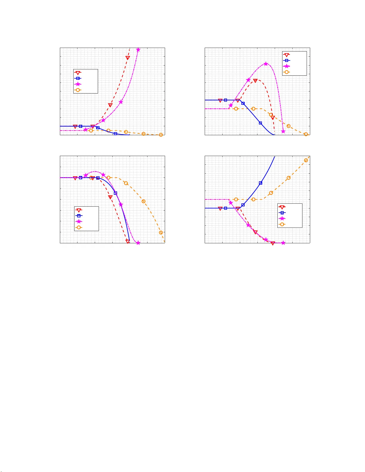
1 Matching Users Preference Under T ar get Re v enue Constraints in Optimal Data Recommendation Sys tems Shanyun Liu, Y unquan Dong, Pingyi Fan, Senior Membe r , IEEE , R ui She, Shuo W a n Abstract This paper foc uses on the problem of ﬁnding a p articular data recomm endation strategy b ased o n the user preferen ces and a sy stem expected revenue. T o this end, we form ulate this prob lem as an optimization by design ing the recommend ation mechanism as close to the user behavior as possible with a certain revenue constraint. In fact, the optim a l recommen dation distribution is the one that is the closest to the u tility distribution in the sense o f relati ve entropy and satisﬁes expec te d revenue. W e show tha t the optimal recom mendation distribution f ollows the same for m a s the message impo rtance measure (MIM) if the target r e ven u e is r easonable, i.e. , neither too small no r too large. Therefo r e, the optimal reco mmendation d istrib ution can be regarded as the normalized MIM, wh ere the parameter, called imp ortance coefﬁcient, presents the concern of th e system and switches the atten tion of the system over data sets with different occurrin g probability . By adjusting the imp ortance coefﬁcient, our MIM b ased framework o f data recommenda tio n can then be ap p lied to system with various system requirem ents and d ata distributions. Therefor e, the ob tained r esults illustrate the p hysical me aning of MIM from th e data recomm endation perspectiv e and validate the ratio n ality of MIM in o ne aspect. Index T erms Data reco mmendation; o p timal recommen d ation distribution; utility distribution; message impo r - tance m e asure; impor tance coefﬁcient. Shanyu n Liu, Rui She, Shuo W an and P ingyi Fan are with Tsinghua National Laboratory for Information Science and T echnology (TNList) and the Department of Electronic E nginee ring, T singhu a University , Beijing, P . R. China, 100084. e-mail: { liushan y16, sher15, wan -s17@mails.tsinghua.edu.cn , fpy@tsinghu a.edu.cn. } Y unquan Dong is with the School of Electronic and Information Eng ineering, Nanjing Unive rsity of Information Science and T echnology , Nanjing, P .R. C hina. email: yunquan dong@nuist.edu .cn This work was suppo rted in part by the National Natural Science Foundation of China (NSFC ) under Grant 61771283, and in part by the China Major State Basic Research Develop ment Program (973 Program) under Grant 2012CB316100(2). 2 I . I N T RO D U C T I O N The data recommendation is one of the m o s t fundamental problems in wireless mob ile Internet, and it becomes more and more crucial in th e era of big data. W ith the explosiv e growth o f data, it is difﬁcult to send all the dat a to the users wit hin tolerable tim e by traditional data processing technology [ 1 ], [ 2 ]. Dat a push or recommendation technology m ay hel p users get their desired information in time. In fact, data can be sent in advance when th e sy s tem is i d le, ev en if there is no ask for it , rather t han wasting ti m e to wait for a clear request from users [ 3 ]. Furthermo re, it is also arduous for users to ﬁnd desired data amo ng a m ass of data a vailable in the Int ernet [ 4 ]. In general, the special data which catches the interests of users can be provided faster and easier with data recommend ation system, since the recommendati o n st rategy is usually well- designed based on the preferences of users explicitly [ 5 ], [ 6 ]. Compared to s earch engines, push is more con venient for less action required, and the quality of data pushed does n ot rely on the skills and knowledge of the users [ 4 ]. For example, many appl ications in mobile phon e prefer to recommend some data based on th e user’ s int erest t o i mprov e the user experience. In additi on, diffe rent from traditional in dustry , the Internet enterprises can make a proﬁt th rou gh m obile network by usi ng push-based advertisement t echno l ogy [ 7 ]. The pre vious works m ainly dis cus sed data push based on the content to solve the problem of data delivery [ 3 ]–[ 10 ]. Data push i s usually regarded as a strategy of data delivery in distributed information systems [ 3 ]. Th e architecture for a m obile push system was proposed i n [ 4 ], [ 8 ]. In addition , [ 9 ] put forward an effecti ve wireless pus h sy stem for h i gh-speed data broadcasting. The push and pull techniques for tim e-v aryin g data network was di s cussed in [ 10 ]. Furthermore, on this basis, the recommendation system was provided as information-ﬁltering system which push data to users based on the knowledge abou t their p references [ 11 ], [ 12 ]. [ 11 ] discussed the joint cont ent recommendation, and the pri vacy-enhancing technology in recommendatio n sys tems was i n vestigated i n [ 12 ]. Besides, [ 13 ] put forward a p ersonalized social image recommendation method. Furthremore, the recommendation technology w as als o u sed to solve the problem in m u ltimedia big data [ 14 ]. Different from t h e preceding works, i n this paper , we do no t discuss the problem of data deliv ery based on content. As an alternative, we shall discuss the distribution of recommendation sequ ence based on the performance of users when the revenue of the recomm endation s y stem is required. Now adays, user customi zation is crucial and it can be so lved by means of recommendation. 3 The personalized concern of user usuall y can be characterized by many properties of the data used b y users, such as data format, keywords [ 4 ], [ 15 ], [ 16 ]. Ho we ver , we choo s e the frequenc y of d at a used to describe the performance of users si n ce it has n othing to do with th e concrete content. In additi o n, we take the rev enu e of t he recommendation sys tem into account. That is, a recommendation process consumes resources while gets beneﬁts. Different recomm endation types may bri n g di fferent resul ts. For example, the cost of omit t ing a data which sho u ld be pushed mistakenly may b e much smaller than that of push i ng in valid d ata to a u ser erroneously . On one hand, the users have conﬁdence in the recommendati on syst em i f th e desired data is pushed to these users correctly . On the other hand, pushing the i n formation that users do not ask, such as advertisement, may seriously i m pact the user experience, but it can st i ll bring re venue from advertisements. T o balance the loss of different types o f push errors, we give diff erent weight to diffe rent types of push errors, which i s similar wi th cost-sensitive l earning [ 17 ]–[ 20 ]. For dif ferent application scenarios, the system focuses on different events according to the need. For example, the small-probabili ty e vents captures our attention in th e minorit y subsets detection [ 21 ], [ 22 ], whil e someone prefers the ev ent wit h high probabil i ty in support vector machine (SVM) [ 23 ]. For applications i n wireless mobil e Internet, i n stage of expanding users, recommending t he desired dat a accurately to attract more users is more im p ortant. Ho we ver , in mature stage, advertising is focused on, since the application s expect to earn more money by advertising though it degrades the user experience. This paper will mainly discuss t hese two cases. There are als o s ome new ﬁndings when the message importance is taken i nto account [ 24 ]– [ 28 ], and message importance can be used to characterize the concern degree of e vents. Message importance measure (MIM) was p rop osed to c haracterize the message importance of e vents which can be described by dis crete random variable where peopl e pa y m ost attenti on to the small-probabili ty ones, and it hig hlights the importance o f minorit y subsets [ 29 ]. In fact, it is an extension of Shannon entropy [ 30 ], [ 31 ] and R ´ enyi entropy [ 32 ] from the perspective of Fadee v’ s postulates [ 32 ], [ 33 ]. That is, t he ﬁrst three p ostulates are satisﬁed for all of them, and MIM weakens the fourth postulate on the foundation of R ´ enyi entropy . Mo reover , t h e logarithmic form and p olynomial form are adopted in Shannon entropy and R ´ enyi entropy , respectively , while MIM uses the exponential form. [ 34 ] showed that MIM focuses on the a speciﬁc event by choosing corresponding importance coef ﬁcient. In fact, MIM has a wide range of applications 4 in big data, such as compressed storage and communication [ 35 ] and mobil e edge computing [ 36 ]. In fact, the superior recommend at i on sequence should like those generated by users, which means that the data recommendation mechanism agrees with user behavior . T o this end, t he probability of observing th e recommendation s equ ence with the utilizati o n frequency of the user data should be as close to one as p ossible i n the statis t ical sense. According to [ 37 ], that means the relative entropy between the dis t rib ution of recommendation sequence and that of user data should be m inimized. W e assume the recommend ation model pursues best user performance with a certain re venue guarantee in this paper . W e ﬁrst ﬁnd a particular recommendation distribution on the best effort i n maximi zing the probability of observing th e recommendation s equ ence with the utilizati o n frequency of the user data when the expected rev enu e is provided. Then, it s main properties, such as monoto n icity and geom etri cal characteristic, are fully discussed. This o p timal recomm end ation syst em can be regarded as an information-ﬁltering system , and the impo rt ance coef ﬁcient determines what e vents the system prefers to recommend. The resul t s also show th at excessiv ely low expectation of re venue can not con strain recommendati on distribution and exorbitant expectation o f revenue makes the recommendation system i mpossible to design. The con straints on the recommendation distribution is true if the minimum av erage revenue is neither too small nor too large, and there is a t radeof f between the recommend at i on accuracy and the expected revenue. It is also noted that the form of this optim al recomm end ation dist ri bution is the s ame as that of M IM when the minimu m avera ge re venue is neither too small nor too large. The optimal recommendation di s trib ution is determined by the proportion of recomm endation value of the correspond i ng ev ent in tot al recommendati on value, where the recommendatio n value is a special weigh t factor . The recom m endation value can be seen as a measure of message importance, si nce it satisﬁes the postulates of the message imp o rtance. Due to th e same form with MIM, the optimal recommendation probability can be give n by t h e norm alized message importance measure when M IM is used to characterize t he concern of system. Furthermore, when importance coefﬁcient is positive, the small-probability ev ents wi l l be taken more attention. That is magnifying the im portance i ndex of small-probabi lity ev ents and lessening that of high- probability ev ents. Therefore, we conﬁrms t he rati onality of MIM from another perspecti ve in this paper for characterizing the physical meaning of MIM by u sing data ecommendatio n system rather than based on information theory . Besides, we expand MIM to the general case wh ate ver 5 the prob ability of sys tems interested events i s. Since the im p ortance coefﬁcient determines what e vents set system s are int erested in, we can switch to different application scenarios by means of it. That is, advertising s y stems are discuss ed if importance coefﬁcient is po s itiv e, while non- commercial systems are adopted if import ance coefﬁcient is negativ e. Compared with previous works about MIM [ 29 ], [ 34 ], [ 35 ], mos t properties of optimal recommendation dist ri bution is the same, but a cl ear deﬁnitio n o f the desi red ev ent set can be giv en in this p aper . The relations h ip between utility distribution and MIM was preli m inarily discussed in [ 38 ]. The main contribution of th is paper can be su mmarized as follows. (1) W e put forward an optimal recomm endation distribution that m ake s th e recommendation mechanism agrees with user behavior with a certain reve nue guarantee, which can improve the desi g n of recommendatio n strategy . (2) W e illuminate that thi s op timal recommendatio n dist ri bution is normalized message importance, when we use M IM to characterize the con cern of system s , w h ich presents a new physical explanation of MIM from data recommendation perspective. (3) W e expand MIM to the general case, and we also discuss the importance coef ﬁcient selection as w el l as its relationship with what e vents systems focus on. The rest o f this paper is organized as follows. The setup of optimal recommendation is introduced in Section II , including the system model and the discussio n of constraints. In Section III , we solve the problem of optimal recommend ati on in our system model, and g ive com plete solutions . Section IV in vestigates the properties of thi s optim al recommendation distribution. The geometric interpretatio n is also discussed in this part. Then, we dis cuss the relationshi p between this opt i mal recommendation di strib ution and MIM in Section V . It is not ed that recommendation distribution can be s een as normalized message im portance in this case. The numerical results is shown and discussed to certiﬁcate our theoretical result s i n Section VI . Section VII concludes the paper . In addit ion, the main notations in this paper are listed in T able. I . I I . S Y S T E M M O D E L W e consider a recommendati on sy stem with N classes of data, as sh o wn in Figure 1 . In fact, data is often s tored based on it s cate gories for the con venience of indexing. For example, the n e ws website usually classiﬁes news into the following categories: politics, entertainm ent, business, scientiﬁc, sports, and so on. At each tim e instant, the information source generates a piece of data, which belongs to a certain class with probabili ty distribution Q and would be similar wi th another probability di s trib ution U . In general, t he generated d at a sequence does not 6 T AB L E I N O T A T I O N S . Notation Description S The set of all the data N The num ber of data classes S i The set of data belong ing to the i -th class S i ∩ S j = ∅ for i 6 = j , and S = S 1 ∪ S 2 ∪ ...S N − 1 ∪ S N Q = { q 1 , q 2 , ..., q N } Raw distribution: the probability distribution of information source P = { r 1 , r 2 , ..., r N } Recommendation distrib ution: t he probability distribution of recommended data U = { u 1 , u 2 , ..., u N } Utility distrib ution: t he probability distribution of user’ s preferred data D ( P k U ) The relati ve entropy or Kullback-Leibler (KL ) distance between P and U C p The cost of a single data push R p The earning when the pushed data is liked by the user C n The cost when the pushed data is not like d by the user R ad The adv ertisi ng reven ue when the pushed data is not l ik ed by the user C m The cost missing to push a piece of user’ s desired data β The target reven ue of a si ngle data push  The importan ce coefﬁcient α α = β + C p − R p R ad − R p − C n − C m γ u γ u = P N i =1 u 2 i g (  , V ) g (  , P ) = P N i =1 v 2 i e  (1 − v i ) P N i =1 v i e  (1 − v i ) f (  , x , U ) f (  , x , U ) = u x e  (1 − u x ) P N i =1 u i e  (1 − u i ) x x = 1 , 2 , · · · , N is the i nde x of classes match the preference of the user . T o optimize the in formation t ransmission process, therefore, a recommendation unit is used to determine whether the generated data shou l d be pushed to the user wit h som e deliberately desi gned probabilit y dis t rib ution U . One the one hand, the recommendation unit can make predictions of the user’ s needs and push some data to the user before he actually starts the retriev al process. In doin g so, the transmi s sion delay can be lar gely reduced, especially when the data amount is large. On the other hand, the recommending u nit enables n on-exper t users to search and to access their desired data much easi er . Furthermore, we can proﬁt more by pu shing some advertisements to t he us er . 7 Push Generate ( ) u t U Recommendation Sequence ( ) p t P Information Sou rces ( ) s t Q 1 S 2 S N S . . . . . . User Message Fig. 1. System model. A. Data Model W e refer to th e emp irical p rob ability mass function of the class ind exes over whole the data set as the raw dist r ib ution and denote i t as Q = { q 1 , q 2 , ..., q N } . W e refer to the probabi lity mass function of users’ preference over the classes as the utility di stribution and denote it as U = { u 1 , u 2 , ..., u N } . That i s, for each pi ece of data, it belo n gs to class i wit h probabili ty q i and would be p referred by the user with probabilit y u i . T o ﬁt the preference of the user under some target revenue constraint, the system will make random recommendat i ons according to a r ecommendation dist rib ution P = { p 1 , p 2 , ..., p N } . W e assum e that each piece of data b elo ngs t o one and only one of the N sets. Th at is, S i ∩ S j = ∅ for ∀ i 6 = j , where S i is the set of data belonging to the i -th class. Thus, the whole data set would be S = S 1 ∪ S 2 ∪ ...S N − 1 ∪ S N . Thus, t h e raw distribution can be expressed as q i = Pr { d ∈ S i } = crad ( S i ) / crad ( S ) . In addition, the utilit y d istribution U can be obtain ed by studying the data-using beha vior of a speciﬁc group of users and th u s is assumed to be known in prior in t his paper . For traditional data pus h , we usually expect to m ak e | u ( t ) − s ( t ) | smaller than a given value [ 10 ]. Diffe rent from t h em, we do not consider this problem based on content. As an alternativ e, our goal is t o ﬁnd the opti mal recommendat i on dist rib ution P so that the recommended data would ﬁt t h e preference of the user as much as po s sible. T o be speciﬁc, each recommended sequence of data sh ould resembl e t h e desi red data sequence of the us er in th e stat i stical sense. For a sequence of user’ s fa vorite data, let u n be the corresponding class i ndex es. As n goes to inﬁnity , it is clear that u n ∈ T ( U ) with probability one, where T ( U ) is t he t y p ical set under distribution U . That i s, Pr { 1 n log Pr( u n ) + H ( U ) = 0 } = 1 , where Pr( u n ) is the occurring probability of u n and H ( U ) is the jo i nt entropy of U [ 37 ]. Since the class-in dex sequence r n of recommended data is actually g enerated wit h distri bution P , the probabilit y that r n falls in 8 the t y pical set T ( U ) of distribution U would be Pr { r n ∈ T ( U ) } . = 2 − nD ( P k U ) , where D ( P k U ) is the relati ve entropy between P and U [ 37 ]. It is clear t h at the optimal P would maximizes probability Pr { r n ∈ T ( U ) } , which is equi valent to m i nimizing the relative entropy D ( P k U ) . (1) In particular , ou r desi red recommendation distribution P is not exactly the same as t he u tility distribution of the user , because we also would like to i ntentionally push some advertisements to the user to i ncrease our proﬁt. B. Revenue Model W e assume that the user di vides the whole data set into two parts, i.e., the desired ones and the unwanted o nes (e.g., adver tisements). At the recommendation unit, the data can also be classiﬁed into two types according to wheth er it is recomm ended to the user . Diff erent push types may strikingly lead t o dif ferent results. For example, the cost of om itting a data which should be pushed m ay be much smaller than that of erroneousl y pushing inv alid data to a user . The user experience wil l be enhanced if th e data needed by users is pushed to them. Pushin g some not need content to users, such as some advertisement, m ay seriously impact the user experience, but it still can bring in advertising re venue for the content delivery enterprise. Us ing a similar re venue model as that in cost-sensitive learnin g [ 17 ]–[ 20 ], we s hall e v aluate the rev enue of th e recommendation system as follows. • The cost of making a recommendation is C p ; • The re venue of a recommendati on when the pushed d ata is liked by the user is R p ; • The cost of a recommendation when the pushed data is no t liked is C n ; • The rev enue of a recomm endation when the pushed data is is not liked (b ut can serve as an advertisement) is R ad ; • The cost of missin g to recommend a pi ece of desired data of the user is C m ; Therefore, the re venue of recommendi ng a piece of data belong i ng to class i can be summarized in the T able II . Moreover , the corresponding matrix of occurring prob ability is given by T able III . 9 T AB L E II T H E R E V E N U E M AT R I X . Preference Action Recommend Not recomen d Desired R p − C p C m Unwanted R ad − C p − C n 0 T AB L E III T H E M A T R I X O F O C C U R R I N G P R O B A B I L I T Y . Preference Action Recommend Not recomen d Desired p i u i (1 − p i ) u i Unwanted p i (1 − u i ) (1 − p i )(1 − u i ) In this paper , we assum e C p , R p , C n , R ad , C m are const raints for a g iven recommendation system for simplicit y . The expected system revenue can then be expressed as R ( P ) = N X i =1 (( R p − C p ) p i u i + ( R ad − C p − C n ) p i (1 − u i ) − C m (1 − p i ) u i ) (2) = − ( R p + C n + C m − R ad )(1 − N X i =1 p i u i ) + R p − C p (3) = − ( R p + C n + C m − R ad ) N X i =1 p i (1 − u i ) + R p − C p . (4) C. Problem F or m u lation In t h is paper , we consider the follo wing three kinds of recommendation systems: 1)the ad- verting system where recomm ending u nwanted advertisements yields higher reve nue; 2) t h e noncommer cial system where recommending user’ s desired data b rings hig her rev enue; 3) the neutral system where the s y s tem rev enu e is independent o f recommend ation probability P . For each giv en tar get re venue constraint R ( P ) ≥ β and each kind of syst em, we shall optim ize the recommendation dist rib ution P by m i nimizing D ( P || U ) . In particular , the following auxiliary var iable is used α = β + C p − R p R ad − R p − C n − C m . (5) 10 1) Advertisi ng Systems: In an advertisi ng s ystem , recommending a piece of user’ s unwanted data (an advertisement ) yields higher reve nue. Since the re venue o f recommending an advertise- ment is the main source of income in this case, which is l ar ger t han ot her revenue and cost, the advertising system would satisfy the fol lo wing condit i on. C 1 : R p + C n + C m − R ad < 0 . (6) By combining ( 4 )–( 6 ), it is clear that the cons t raint R ( P ) ≥ β is equiv alent to N X i =1 p i (1 − u i ) ≥ α. (7) For advertising sys tems, therefore, the feasible set of recommendation d istribution P can be expressed as E 1 = n P : X N i =1 p i (1 − u i ) ≥ α | R ad > R p + C n + C m o . (8) For a given target revenue β , we shall s o lve the optimal recommendati on distribution P of advertising system s from P 1 : arg min P ∈ E 1 D ( P k U ) (9) s.t. N X i =1 p i (1 − u i ) ≥ α (9a) N X i =1 p i = 1 . (9b) 2) Noncommer cia l Systems: A noncommer cial system is deﬁned as a recommendati on system where the rev enue R p − C p of recommending a piece of desi red data is larger than the s u m of re venue R ad − C p − C n of recommendin g an advertisement and the cost of not recommendi ng a piece of desired data C m . That is, C 2 : R p + C n + C m − R ad > 0 . (10) Accordingly , the constraint R ( P ) ≥ β is equiv alent to N X i =1 p i (1 − u i ) ≤ α. (11) Therefore, the feasible s et of recommendation di strib ution P for non commercial systems can be expressed as E 2 = n P : X N i =1 p i (1 − u i ) ≤ α | R ad < R p + C n + C m o . (12) 11 Afterwards, we can solve the optimal recommendation distribution P throu gh the following optimizatio n problem. P 2 : arg min P ∈ E 2 D ( P k U ) (13) s.t. N X i =1 p i (1 − u i ) ≤ α (13a) N X i =1 p i = 1 . (13b) 3) Neutral Systems: For the case R p + C n + C m − R ad = 0 , the correspondi n g expected system re venue degrades to R ( P ) = R p − C p (14) and is independent from the recommendation distri bution P . As lo n g as the t arget rev enue satisﬁes β < R p − C p , the const raint R ( P ) ≥ β can b e m et by any recommendation di stribution. Therefore, the recommendation distribution can be chosen as P = U . 4) Discuss ion of S ystems: Noncommercial systems usual l y appear in stage of expanding users. In t h is stage, in order to seize market share, the main tasks are attracting more users and making u sers have conﬁdence i n this recommendation system s by excellent user experience, and therefore the re venue from new us ers by recommending desired data should be lar ger than the re venue of recommending an advertisement and the cost of not recommending a piece o f desired data. Generally , from a qualitative perspectiv e, th e data desired by users with h i gh-probability is recommended with high er probability to make R ( P ) lar g er in this case, since R ( P ) decreases with increasing of P N i =1 p i (1 − u i ) . In thi s sense, the high-probabi lity e vents are m o re important here. Advertising systems is usually adopted in matu re stage of applications wh ere users are ac- customed to the recommendatio n system and can put up with som e advertisements. Here, the applications expect t o earn more money by advertising. Thus, the revenue of recommendi n g an advertisement is lar ger than other re venue and cost in advertising system s. From a qualitative perspectiv e, in order to get more rev enue, th e data desired by users with sm all-probability (e.g., advertisements ) should be recomm ended with high probability since R ( P ) increases with increasing of P N i =1 p i (1 − u i ) . In this sense, the small-probabili ty eve nts are m ore important here. 12 Remark 1 . Since n P : R ( P ) ≥ β o = E 1 ∪ E 2 ∪ n P : R ( P ) ≥ β | R ad = R p + C n + C m o , t h ese three kinds of recommendation s ystems cover all the cases of this problem. I I I . O P T I M A L R E C O M M E N DA T I O N D I S T R I B U T I O N In this p art, we sh all present the optimal recommendati on distribution for both advertising systems and n o ncommercial systems explicitly . W e deﬁne an auxiliary v ariable and an auxiliary function as follows. γ u = X N i =1 u 2 i , (15) g (  , V ) = P N i =1 v 2 i e  (1 − v i ) P N i =1 v i e  (1 − v i ) , (16) where  ∈ ( −∞ , + ∞ ) is a constant and V = { v 1 , v 2 , · · · , v N } is a general probability mass function. Actually , we have γ u = e − H 2 ( U ) where H 2 ( U ) is the R ´ enyi entropy H α ( · ) when α = 2 [ 40 ]. In parti cul ar , we ha ve the following lemma on g (  , V ) . Lemma 1 . Function g (  , V ) is m o notonically decreasing with  . Pr oof. Refer to Appendix A . Lemma 2 . g (0 , V ) = P N i =1 v 2 i , g ( −∞ , V ) = v max , and g (+ ∞ , V ) = v min , where v max = max { v 1 , v 2 , · · · , v N } and v min = min { v 1 , v 2 , · · · , v N } . Pr oof. Refer to the Appendix B It i s clear that we hav e g (0 , P ) = γ p and g (0 , U ) = γ u . A. Optimal Advertising Syst em Theor em 1 . For an advertising system wi th R p + C n + C m − R ad < 0 , the optim al recommendation distribution is the solution of Problem P 1 and is giv en by p ∗ x =              u x if α ≤ 1 − γ u u x e  ∗ (1 − u x ) P N i =1 u i e  ∗ (1 − u i ) if 1 − γ u < α ≤ 1 NaN if 1 ≤ α (17) for 1 ≤ x ≤ N , where α is deﬁned in ( 5 ), γ u is deﬁned in ( 15 ), NaN means no so l ution exists, and  ∗ > 0 is the solution to g (  , U ) = 1 − α . 13 Pr oof. First , if α > 1 , no solution exists since P N i =1 p i (1 − u i ) is alw ays small er than one and the constraint ( 9a ) can nev er be satisﬁed. Second, if α ≤ 1 − γ u , w e have P N i =1 p i (1 − u i ) ≥ P N i =1 u i (1 − u i ) = 1 − γ u ≥ α . That is, the con s traint ( 9a ) coul d by satisﬁed with any d i stribution P . Th us, the solu t ion to Problem P 1 would be P = U , which m inimizes D ( P || U ) . Third, if 1 − γ u < α ≤ 1 , we s h all solve Problem P 1 based on the following Karush-Kuhn- T ucher (KKT) conditions. ∇ P L ( P , λ, µ ) = ∇ P N X i =1 p i ln p i u i + λ α − N X i =1 p i (1 − u i ) ! + µ N X i =1 p i − 1 !! =0 (18) λ ( α − N X i =1 p i (1 − u i )) =0 (18a) N X i =1 p i − 1 = 0 (18b) α − N X i =1 p i (1 − u i ) ≤ 0 (18c) λ ≥ 0 (18d) Diffe rentiating ∇ P L ( P , λ, µ ) with respect to p ∗ x and set it to zero, we have ln p ∗ x + 1 − ln u x − λ (1 − u x ) + µ = 0 , (19) and thus p ∗ x = u x e λ (1 − u x ) − µ − 1 . T ogether with cons t raint ( 18b ), we furth er have e µ +1 = P N i =1 u i e λ (1 − u i ) and p ∗ x = u x e λ (1 − u x ) P N i =1 u i e λ (1 − u i ) , (20) where λ ≥ 0 is the solution to P N i =1 p ∗ i (1 − u i ) = α , i.e., g ( λ , U ) = 1 − α . By substituting λ with  ∗ , the d esired resul t in ( 17 ) would be ob t ained. The cond i tion 1 − γ u < α ≤ 1 implies g (  ∗ , U ) = 1 − α ≤ γ u = g (0 , U ) . Since g (  , U ) has been shown to be monoto n ically decreasing with  in Lemma 1 , we then hav e  ∗ > 0 . T h is completes the p roo f of Theorem 1 . Remark 2 . W e denote β 0 =(1 − γ u )( R ad − R p − C n − C m ) + R p − C p , (21) β ad = − ( R ad − R p − C n − C m ) u min + R ad − C p − C n − C m , (22) 14 and hav e • α ≤ 1 − γ u is equiv alent to β ≤ β 0 , which means that the target rev enu e is low and can be achie ved by pushing data according to t he preference of the user exactly . • 1 − γ u < α ≤ 1 is equiv alent to β 0 < β ≤ β ad , which means that t h e tar get rev enue can only be achie ved when some advertisements are pushed according to probability p ∗ x . • 1 < α is equiva lent to β > β ad , which means that t h e tar get is too high to achieve, even when advertisements are pushed with probability one. B. Optimal Noncommer cial System Theor em 2 . For a n oncommercial s ystem with R p + C n + C m − R ad > 0 , the optim al recom- mendation distribution is the solution of Problem P 2 and i s g iven by p ∗ x =              NaN if α < 0 u x e  ∗ (1 − u x ) P N i =1 u i e  ∗ (1 − u i ) if 0 ≤ α < 1 − γ u u x if 1 − γ u ≤ α , (23) for 1 ≤ x ≤ N , where α is deﬁned in ( 5 ), γ u is deﬁned in ( 15 ), NaN means no so l ution exists, and  ∗ < 0 is the solution to g (  , U ) = 1 − α . Pr oof. First , if α < 0 , no solution exists s i nce P N i =1 p i (1 − u i ) is p o sitiv e and cannot be smaller a negati ve nu m ber , and thus the constraint ( 13b ) can nev er be satisﬁed. Second, if α ≥ 1 − γ u and we set p ∗ x = u x , we would ha ve P N i =1 p ∗ i (1 − u i ) = 1 − γ u ≤ α , i.e., constraint ( 13a ) i s satisﬁed. Since setting p ∗ x = u x minimizes D ( P | | U ) , P = U shou ld be the solution of Problem 2. 15 Third, if 0 ≤ α < 1 − γ u , we shall solve Problem P 2 using the fol lo wing KKT condi tions. ∇ P L ( P , λ, µ ) = ∇ P N X i =1 p i ln p i u i + λ N X i =1 p i (1 − u i ) − α ! + µ N X i =1 p i − 1 !! =0 (24) λ ( N X i =1 p i (1 − u i ) − α ) =0 (24a) N X i =1 p i − 1 = 0 (24b) N X i =1 p i (1 − u i ) − α ≤ 0 (24c) λ ≥ 0 (24d) Diffe rentiating ∇ P L ( P , λ, µ ) with respect to p ∗ x and s et i t to zero, we have ln p ∗ x + 1 − ln u x + λ (1 − u x ) + µ = 0 , (25) and p ∗ x = u x e − λ (1 − u x ) − µ − 1 . T ogether with constraint ( 24b )), we then ha ve e µ +1 = P N i =1 u i e − λ (1 − u i ) and p ∗ x = u x e − λ (1 − u x ) P N i =1 u i e − λ (1 − u i ) , (26) where λ > 0 is the soluti o n to P N i =1 p ∗ i (1 − u i ) = α . By denot i ng  ∗ = − λ , ( 26 ) turns to be p ∗ x = u x e  ∗ (1 − u x ) P N i =1 u i e  ∗ (1 − u i ) which is the desired result in ( 23 ). Moreover , the condition 0 ≤ α < 1 − γ u implies g (  ∗ , U ) = 1 − α ≥ γ u = g (0 , U ) . Since g (  , U ) is mo n otonically decreasing with  (cf. Lemma 1 ), we see that  ∗ < 0 . Thus , T h eorem 2 is prove d. Remark 3 . W e denote β no = − ( R ad − R p − C n − C m ) u max + R ad − C p − C n − C m , (27) and hav e the following observations. • α < 0 is equiv alent to β ≥ β no , which means that t h e tar get rev enue is hig h and cannot b e achie ved by any recommendati o n distri bution. • 0 ≤ α < 1 − γ u is equiv alent to β 0 < β ≤ β no , which means that the target re venue is n o t too hig h and the information is pushed according to probability p ∗ x . Th e user experience is limited by th e target re venue in this case. 16 • 1 − γ u ≤ α is equiv alent to β ≤ β 0 , w h ich can be achieved by pushin g data according to the p refere nce of the user exactly . C. Sh o rt Summar y W e further denote β ne = R p − C p , (28) the o ptimal recommendation dis t rib utions for various system s and var ious target revenues can then be summarized in T able IV . T AB L E IV T H E O P T I M A L R E C O M M E N DAT I O N D I S T R I B U T I O N . Case β α p ∗ x Advertising system 1  β ≤ β 0 α ≤ 1 − γ u x 2  β 0 < β ≤ β ad 1 − γ < α ≤ 1 u x e  (1 − u x ) P N i =1 u i e  (1 − u i ) 3  β > β ad α > 1 NaN Neutral system 4  β ≤ β ne NaN u x 5  β > β ne NaN NaN Noncommercial system 6  β 0 < β ≤ β no 0 ≤ α < 1 − γ u x e  (1 − u x ) P N i =1 u i e  (1 − u i ) 7  β ≤ β 0 α ≥ 1 − γ u x 8  β > β no α < 0 NaN Cases 3  , 5  , and 8  are extreme cases where the t ar get rev enue is beyond the reach of the system. For cases 1  , 4  , and 7  , the target re venue is low ( β < β no or β < β ad ), and thus is easy to achieve. In p articular , the constraints ( 9a ) and ( 13a ) are actually inactive . T h us, the optimal recommendation distribution would be exactly the same with t he ut ility dist rib ution. Cases 2  and 6  are more practical and m eanin gful due to the appropriate target re venues used. T o further s t udy the prop erty of th e opti mal recommendation distribution of these two cases, the following function i s i ntroduced, f (  , x, U ) = u x e  (1 − u x ) P N i =1 u i e  (1 − u i ) , (29) where  ∈ ( −∞ , + ∞ ) . In doing so, the opt i mal recomm endation dist rib ution o f cases 2  and 6  can be jointl y expressed as p ∗ x = f (  ∗ , x, U ) , (30) 17 where  ∗ is the solution to g (  , U ) = 1 − α . In particular , f (  ∗ , x, U ) presents the optimal solution of case 2  if  ∗ > 0 and presents the solution of case 6  if  ∗ < 0 . Moreover , when  = 0 , we ha ve f (0 , x, U ) = u x , (31) which can be cons idered as th e solutio n to cases 1  , 4  , and 7  . I V . P RO P E RT Y O F O P T I M A L R E C O M M E N DAT I O N D I S T R I B U T I O N S In thi s section, we shall in vestigate how the o ptimal recomm endation distribution diver ges with respect to the utility dist ri bution, in va rious system s and under various target rev enue constraints. T o do so, we ﬁrst study the property of function f (  , x, U ) , where  x and e  x 6 = 0 are, respecti vely , the solution to the following equations u x = g (  , U ) , (32) u x = f (  , x, U ) . (33) A. Monotonicity of f (  , x, U ) Theor em 3 . f (  , x, U ) h as t he following properties. 1) f (  , x, U ) is monotonically i ncreasing w i th  in ( −∞ ,  x ) ; 2) f (  , x, U ) is monotonically d ecreasing wi th  in (  x , + ∞ ) ; 3)  x is decreasing with u x , i.e,  y <  x if u y > u x ; 4)  x < 0 if u x > γ u ;  x = 0 if u x = γ u ;  x > 0 if u x < γ u . Pr oof. 1 ) and 2) The deriv ative of (  , x, U ) with respect to  can be expressed as ∂ ( f (  , x, U )) ∂  = u x e  (1 − u x ) (1 − u x ) P N i =1 u i e  (1 − u i ) − u x e  (1 − u x ) P N i =1 u i e  (1 − u i ) (1 − u i )  P N i =1 u i e  (1 − u i )  2 (34) = u x e  (1 − u x ) P N i =1 u i ( u i − u x ) e  (1 − u i )  P N i =1 u i e  (1 − u i )  2 . (34a) Since we hav e u x e  (1 − u x ) > 0 and  P N i =1 u i e  (1 − u i )  2 > 0 , the sign of t he d eriva tiv e only depends on the t erm P N i =1 u i ( u i − u x ) e  (1 − u i ) . 18 Lemma 1 and Lemma 2 show that g (  , U ) is monot o nically decreasing with  and  x is the unique soluti o n to equation u x = g (  , U ) . For  <  x , therefore, we then have g (  , U ) > g (  x , U ) = u x , which is equiv alent to P N i =1 u i ( u i − u x ) e  (1 − u i ) > 0 . Thus, we h a ve ∂ ( f ( ,x,U )) ∂  > 0 and f (  , x, U ) is i ncreasing wit h  if  <  x . Like wise, it can be readily proved that f (  , x, U ) i s d ecrea sing with  if  >  x . 3) Suppose g (  x , U ) = u x , g (  y , U ) = u y and u x  y , i.e.,  x is decreasing with u x . 4) First, we have g ( 0 , U ) = γ u by the deﬁnit ion of g (  , U ) (cf. ( 16 )). Usi n g the m onotonicity of g (  , U ) with respect to  (cf. Lemma 1 ), we hav e  x < 0 if u x > γ u and  x > 0 if u x < γ u . Thus, the proo f of Theorem 3 is completed. In particul ar , according to Lemma 2 , if u x = u min ,  x will approach positive inﬁnity , while  x will approach negati ve inﬁnity if u x = u max . Remark 4 . 1) f (  , x, U ) is m o notonously decreasing with  if u x = u max ; 2) f (  , x, U ) is monotonous ly increasing wit h  if u x = u min . Remark 5 . W e denote β x = − ( R ad − R p − C n − C m ) u x − C p − C n − C m + R ad , (35) and the relationships bet w een f (  , x, U ) and β in differe nt systems are shown as follows. • For advertising systems, 1) f (  , x, U ) is m o notonically decreasing with β in ( β 0 , β ad ) if u x ≥ γ u ; 2) f (  , x, U ) is mon o t onically i ncreasing wi th β in ( β 0 , β x ) and monotonically decreas- ing in ( β x , β ad ) if u x < γ u . • For noncom mercial system s , 1) f (  , x, U ) is m o notonically decreasing with β in ( β 0 , β no ) if u x ≤ γ u ; 2) f (  , x, U ) is mon o t onically i ncreasing wi th β in ( β 0 , β x ) and monotonically decreas- ing in ( β x , β no ) if u x < γ u . B. Discussion of P arameter Assume that there is unique minim um p min and unique maximum p max in utilit y dist rib ution U . W ithout loss of generality , let u 1 < u 2 ≤ ... ≤ u t ≤ γ u < u t +1 ≤ ... ≤ u N − 1 < u N , and 19 u min = u 1 and u max = u N . P ∗ = ( p ∗ 1 , p ∗ 2 , ..., p ∗ N ) is used t o d eno t e the optimal recommendation distribution. Besides, we only discuss the relatio n ship between the opt imal recommendation distribution and the parameters ( β and  ) in Cases 2  and 6  in this part. In fact, we have the following propositi o n on e  x . Pr oposi tion 1 . e  x has the following properties. 1) e  x exists when u x 6 = γ u , u x 6 = u max and u x 6 = u min ; 2) e  x < 0 if u x > γ u ; e  x > 0 if u x < γ u . 3) e  x is decreasing with u x , i.e, e  y < e  x if u y > u x ; Pr oof. Refer to the Appendix C . For con venience, we denote e  1 ∆ = + ∞ and e  N ∆ = −∞ . For advertising syst em s, th e optimal recommendation distribution is give n by ( 17 ) and  ∗ > 0 (cf. Theorem 1 ). As  ∗ → + ∞ , we ha ve p ∗ 1 = f (+ ∞ , 1 , U ) = lim  ∗ → + ∞ u min e  ∗ (1 − u min ) P N i =1 p i e  ∗ (1 − u i ) (36) = lim  ∗ → + ∞ u min e  ∗ (1 − u min ) u min e  ∗ (1 − u min ) + P u i 6 = u min u i e  ∗ (1 − u i ) (36a) = lim  ∗ → + ∞ 1 1 + P u i 6 = u min u i u min e  ∗ ( u min − u i ) (36b) =1 . (36c) Obviously , p ∗ k = f (+ ∞ , k , U ) = 0 when k ≥ 2 . Therefore, the utility di stribution P ∗ is (1 , 0 , 0 , ..., 0) h ere. Based on Proposit ion 1 , if 0 < e  N 3 +1 <  ∗ < e  N 3 ( 1 ≤ N 3 ≤ N − 1 ), we have p ∗ x > u x for 1 ≤ x ≤ N 3 and p ∗ x < u x for N 3 + 1 ≤ x ≤ N . The number of optimal recommendation probability whi ch is larger than correspondi n g utility probabili ty is N 3 . Let N 4 = N − N 3 . N 3 decreases with increasing of  ∗ (cf. Proposition 1 ). In particular , if  ∗ > e  2 > 0 , only the recommendation p robability of the ev ent with smallest utili t y probability is enlarged and t hat of other eve nts is reduced, compared to the corresponding uti lity probabi lity . As the parameter  ∗ approaches posi t i ve inﬁnity , the recommendation distribution wil l be (1 , 0 , 0 , ..., 0) . In con clu sion, this recommendation system is a special inform ation-ﬁltering system which prefers to push the small-probabili ty events. 20 For noncom mercial syst ems, we can get the optimal recommendation dis trib ution b y ( 23 ) and  ∗ < 0 (cf. Theorem 2 ). As  → −∞ , it is no ted that p ∗ N = f ( −∞ , N , U ) = lim  →−∞ u max e  (1 − u max ) P N i =1 u i e  (1 − u i ) (37) = lim  →−∞ u max e  (1 − u max ) u max e  (1 − u max ) + P u i 6 = u max u i e  (1 − u i ) (37a) = lim  →−∞ 1 1 + P u i 6 = u max u i u max e  ( u max − u i ) (37b) =1 , (37c) and p ∗ k = f ( −∞ , k , U ) = 0 when k ≤ N − 1 . Hence, P ∗ = (0 , 0 , .., 0 , 1 ) in this case. If e  K +1 <  < e  K < 0 ( 1 ≤ K ≤ N − 1 ), p ∗ x u x for K + 1 ≤ x ≤ N . The number of optim al recommend ation probability which i s larger th an corresponding utilit y probabili ty is N − K . Let N 2 = N − K and N 1 = K . It is noted t hat N 2 decreases with decreasing of  (cf. Proposition 1 ). In particular , if  < e  N − 1 < 0 , only the recommendatio n probability of the event with lar gest uti l ity probability is enlar ged and that of other e vents is reduced, compared to t he correspondi ng utility probability . As the parameter  approaches negative inﬁnit y , the push distribution will be (0 , 0 , ..., 0 , 1) . In this case, the high-probabilit y events are prefered to push by this recommendation system. Let the optimal recommendation distribution be equal to the utility distribution, i.e., P ∗ = U , and we ha ve u j = u j e  (1 − u j ) P N i =1 u i e  (1 − u i ) = f (  , j, U ) , 1 ≤ j ≤ N . (38) It is noted that  = 0 is the solutio n of ( 38 ) according to ( 31 ). Since f (  , 1 , U ) is m onotonously increasing with  (cf. Remark 4 ), f (  , 1 , U ) 6 = f (0 , 1 , U ) = u 1 when  6 = 0 . Thus there exists one and o n l y one root for ( 38 ), which is  = 0 , and P ∗ = U i n this case. Here, all the data types are fairly treated. For conv enience, the relationship between parameter , the optim al recomm end at i on distribution and the utility d i stribution is summarized in T able V . In fact, the recommendation system can be regarded as an information-ﬁltering system which push data based on the preferences of users [ 12 ]. The i nput and ou t put of this informatio n- ﬁltering sy s tem can be seen as util ity dist ri b u t ion and optimal recommendation di s trib ution, 21 T AB L E V O P T I M A L R E C O M M E N DAT I O N D I S T R I B U T I O N W I T H PA R A M E T E R S . ↓ I S U S E D T O D E N O T E p ∗ x u x . β  x = 1 2 ≤ x ≤ t t + 1 ≤ x ≤ N − 1 x = N P ∗ β no −∞ 0 p ∗ x u N ( ↓ , ..., ↓ | {z } N 1 , ↑ , ..., ↑ | {z } N 2 ) ( β 0 , ˜ β x ) ( −∞ , e  x ) / / p ∗ x u N ( ˜ β x , β no ) ( e  x , 0) / / p ∗ x > u x p ∗ N > u N β 0 0 p ∗ 1 = u 1 p ∗ x = u x p ∗ x = u x p ∗ N = u N ( u 1 , u 2 , ..., u N ) ( β 0 , ˜ β x ) (0 , e  x ) p ∗ 1 > u 1 p ∗ x > u x / / ( ↑ , ..., ↑ | {z } N 3 , ↓ , ..., ↓ | {z } N 4 ) ( ˜ β x , β ad ) ( e  x , + ∞ ) p ∗ 1 > u 1 p ∗ x u 1 / p ∗ x < u x p ∗ N < u N β ad + ∞ 1 p ∗ x < u x p ∗ x < u x 0 (1,0,...,0,0) respectiv ely . For advertising systems , com pared to the input, on the o u tput port, the recommen- dation probabi lity of data belo n g ing to th e set { S i | 1 ≤ i ≤ K } is ampliﬁed, and that belong i ng to the set { S i | K + 1 ≤ i ≤ N } is miniﬁed, where 1 ≤ K ≤ N − 1 and 0 < e  K +1 <  < e  K . Since u 1 < u 2 ≤ ... ≤ ... ≤ u N − 1 < u N , the advertising sy s tem is a special informati on-ﬁltering system whi ch prefers t o push th e small -prob ability ev ents. Assum e e  K +1 <  < e  K < 0 and 1 ≤ K ≤ N − 1 . F or noncomm ercial sy s tems, the data w i th higher utili ty probabil ity , i.e., { S i | K + 1 ≤ i ≤ N } , is more likely to be pus h ed, and th e data with smaller utili ty probability , i.e., { S i | 1 ≤ i ≤ K } , tends to be ov erlooked. Since u 1 < u 2 ≤ ... ≤ ... ≤ u N − 1 < u N , the high-probabilit y events are prefered to push by the advertising syst em . Remark 6 . The recommendation sys t em can be regarded as an information -ﬁltering system, and parameter  i s li ke a indicator which can reﬂect the system performance. If  > 0 , the system is a advertising system, which prefers to recomm end the s mall-probability ev ent s, while the s ystem is a noncommercial system , which is more likely to recommend the high-probabil i ty ev ents if  < 0 . In particular , t he system pushes data according to the preference of the user exactly if  = 0 . C. Geometr i c Interp retation In this part, we will give a geometric interpretation of opti mal recommend ation di s trib ution by means of probabilit y sim plex. Let P denote all the probabili t y dist rib utions from an alphabet 22 U * P P 3 2 6 1 7 8 4 5 A 1 A B 1 B C 1 C Neutral Systems 0 p n m ad R C C R + + - < 0 p n m ad R C C R + + - > 0 p n m ad R C C R + + - = Fig. 2. Probability simplex and optimal recommen dation. Region i  deno tes Case i  in T able III for 1 ≤ i ≤ 8 . { S 1 , S 2 , ..., S N } , and point U denote the ut i lity d istribution. Besides, P is notati o n t o denote recommendation d istribution and P ∗ denotes the opti mal recommendation distribution. W ith the help of the method of types [ 37 ], we hav e Figure 2 to characterize the generation of o p timal recommendation distribution. In Figure 2 , all cases can be grouped into three major categories, i.e., R p + C n + C m − R ad < 0 , R p + C n + C m − R ad = 0 and R p + C n + C m − R ad > 0 . In fac t, these three cate gories are advertising sys tems, neutral systems and noncommercial systems, which are denoted by triangles ∆ AB U , ∆ B C U and ∆ AC U , respectively . Triangles ∆ A 1 B 1 C 1 denotes the region where the av erage re venue is equal or l arger than a giv en value. In this paper , o ur goal is to ﬁnd the opti m al recommendation dist rib ution so that the recommended data would ﬁt the preference of the user as m uch as possible when the a verage re venue satisﬁes t h e predeﬁned requirement. Sin ce the matching degree between the recommended d ata and the user’ s performance is characterized by 2 − nD ( P k U ) (cf. Section II-A ), P ∗ should be a recommendation di s trib ution o n the border of or in the triangles ∆ A 1 B 1 C 1 , which i s closest to utilit y dist rib ution U in relative ent ropy . Therefore, there is no solution if recommendation di strib ution P falls withi n region 3  , 5  and 8  . For advertising systems, P can be divided int o region 1  2  3  . O bviou s ly , P ∗ = U for region 1  since U falls within region 1  . P ∗ in 2  is the recommend at i on distribution closest to U in relative entropy . It is not ed that 2 − nD ( P ∗ k U ) > 2 − nD ( P k U ) if P 6 = P ∗ and P ∈ 2  . There is 23 no solut i on in region 3  since P / ∈ ∆ A 1 B 1 C 1 . There is a simi lar si tuation for noncommercial systems, which is comp o s ed of region 6  , 7  and 8  . There are only two regions for n eut ral systems.In this case, t here is no solut ion when P ∈ 5  , and P ∗ = U when P ∈ 4  . Furthermore, Triangles ∆ AB U characterizes the s et E 1 and triangles ∆ AC U characterizes t he set E 2 . V . R E L A T I O N S H I P B E T W E E N O P T I M A L R E C O M M E N DAT I O N S T R A T E G Y A N D M I M A. Normalized Recommendat ion V al ue In this section, we shall focus on the relationship between opt imal recomm endation distribution and MIM in Cases 2  and 6  . In f act, the optimal recommendation di s trib ution in other cases is in variable and it makes little sens e to discuss the relationship between them. W ithin a period of ti me, the parameters C p , R p , C n , R ad , C m can be seen as in variants of the recommendation system for a given system, and they do not change with the us ers. The strategy recommendation is determined by th e personalized user concern and the expected rev enue in this paper . T h e former is characterized by the utilit y distirbution, and the latter is denoted by β . Based on the discussion in Section III-C , there is one-to-one mappin g between t h e parameter  and the m inimum ave rage re venue β . Thus, o nce the recommendation en vironment is determined, we only need t o s elect the proper parameter  ∗ to get the opti mal recommendati o n di stribution based on the util i ty dist rib ution, and here  ∗ is chosen to satisfy the expectation of the avera ge re venue. The form of optimal recommendation distribution in ( 29 ) suggests that we allocate recom- mendation proportion by weight factor u i e  ∗ (1 − u i ) where U = { u 1 , u 2 , ..., u N } is the uti lity distribution. In a sense, we take th e weigh t factor u i e  ∗ (1 − u i ) as the recommendation value of data belon g ing to the i -th class, and we generate optimal recommendation distribution based on the recomm endation value. It is noted that the o p timal recommendatio n distri bution is the normalized recommendation value. Furtherm o re, the total recommendation value of thi s user is P N i =1 u i e  (1 − u i ) . In fact, the recommendation values are the subjective vi ew , and they are not objective quantit y in nature. They show the relativ e lev el of recommendation tendency . If all the recommendation values m u ltiply by the same constant , the suggested recommend at i on di s trib ution will not change. 24 B. Optimal Recommendation and MIM Generally speaking , there mus t be a reason of th e fact thar the recommendation strategy prefers speciﬁc data. According to the d i scussion in Remark 6 , advertising systems prefer the sm all-probability ev ents (i. e., advertisement), Th e system push as many small -probability e vents as possible with the increasing of the mi n imum a verage reve nuen since pushing small- probability ev ents is the main source of income for this system. Noncommercial systems prefer the hig h -probability events, and they pu s h as m an y high-probabil i ty e vents as possi ble wit h the in creasing of the minim um a verage rev enue since recommending a piece of d esired data is the main source of income for thi s s ystem. The preference of the recomm end ation sys tem means that the system has its own ev aluat i on of the degree of importance for d if ferent d ata. The system p refers to recommend the important data in order to achie ve t he recommendation tar get in our model. Thus, the recommendatio n di s trib ution is determined by the importance of data. Th at is, the recommendation probabilit y of d ata belongi n g to the i -th class is the proportion of recommendation v alue u i e  ∗ (1 − u i ) in total recommendation v alue. In this sense, the recommendation value gives intu i ti ve description of message importance. Furthermore, their relativ e magni tudes are more signiﬁcant than their absolute m agnitude. F or a given parameter , the recommendation value i s a quanti ty wi th respect to probability distribution. Hence, the recommendation v alu e can be seen as a measure of message im portance from t his viewpoint, which agrees with the main general principles for deﬁnition of impo rt ance in previous lit eratures [ 24 ]–[ 28 ]. Moreover , t h e total recomm endation v alu e characterizes the total message im p ortance. In fact, the form of this importance measure is extremely similar to that of MIM [ 29 ]. MIM is proposed to m easure the message importance i n the case where small -probability events contains most valuable inform at i on and the parameter  in MIM is called im p ortance coefﬁcient . The importance coefﬁ cient i s always larger than zero i n MIM. Furthermore, the MIM highl ights the importance of min ority subs ets and i g nores t h e high -probability e vent by taking them for g rant. As stated in Remark 6 , the small-probabili ty ev ents are highlig h ted when  > 0 . Therefore, MIM is cons istent wi th the conclusion of this paper . Besides, as the parameter i ncreased to sufﬁciently large, the message im portance of the ev ent with m inimum probabi l ity dominates the MIM according to [ 29 ], [ 35 ]. It is the same with recommendation value since lim  → + ∞ u min e  (1 − u min ) P N i =1 p i e  (1 − u i ) = 1 (cf. ( 36 )). Furthermo re, if  is not a very lar ge p o s itiv e num ber , the form of f (  , x, P ) ( 1 < x < N ) is similar with Shannon entropy , 25 which is dis cus sed in [ 39 ]. [ 34 ] di s cussed the selection of importance coefﬁcient, and it pointed out that the eve nt with probability u j becomes the princip al compo nent i n MIM when  = 1 /u j . Due t o the same form, the optimal recommendati on distribution also has thi s conclusion. That is, f (1 /u j , j, U ) is the l arger than f (1 /u j , i, U ) if i 6 = j , which i s sho wn in Fig. 6 . Remark 7 . The optimal recommendati on probabilit y is norm alized message importance by means of M IM. In other word, the normalized message i mportance can also be seen as a distribution that is closest t o ut ility dist rib u tion in relativ e entropy , when the ave rage re venue of this recom- mendation system is equal o r l arger than a predeﬁned value. Although the MIM is proposed b ased on information theory , it can also be giv en from the viewpoint of data recomm endation. In fact, Remark 7 characterizes the physical meaning of MIM from data recom m endation perspective, which conﬁrms the rationality of MIM in one aspect. Remark 8 . W e als o expands MIM to general cases whatev er the probability of users interested e vent is. The i mportance coef ﬁcient  plays a switch role o n the event sets of users attention , that is 1) If  > 0 , th e importance index of sm all-probability ev ent s is m agn i ﬁed while that of high-probabilit y ev ents is lessened. In this case, the system prefers to recommend the small-probabili ty ev ent s; 2) If  < 0 , the importance in d e x of hi g h-probability events i s magni ﬁed wh ile th at of small-probabili ty e vents is lessened. In t h is case, the system prefers to recommend the high-probabilit y e vents; 3) If  = 0 , Th e importance of all ev ents is th e same. Besides, the value of this parameter  can also give a clear deﬁniti on of the set which users are interested in. For example, for a gi ven utility d i stribution U ( u 1 < u 2 ≤ ... ≤ u N − 1 < u N ), i f 0 < e  K +1 <  < e  K ( 1 ≤ K ≤ N − 1 ), the sparse events are focused on, and the set of these e vents is { S i | 1 ≤ i ≤ K } here. In fact, { S i | 1 ≤ i ≤ K } give a unambigu o u s description of the deﬁnition of sm all-probability ev ent s in MIM. On the contrary , { S i | K ≤ i ≤ N } is the set of the e vents with hig h -probability which i s highligh t ed if e  K +1 <  < e  K < 0 ( 1 ≤ K ≤ N − 1 ). In particular , if  > e  2 > 0 , only the ev ents wi th min imum probability will be focused on. 26 -100 -80 -60 -40 -20 0 20 40 60 80 100 P arameter  0 0.1 0.2 0.3 0.4 0.5 0.6 0.7 0.8 0.9 1 The function g ( , P ) P = { 0 . 1 , 0 . 2 , 0 . 3 , 0 . 4 } P = { 0 . 05 , 0 . 15 , 0 . 3 , 0 . 5 } P = { 0 . 13 , 0 . 17 , 0 . 34 , 0 . 36 } P = { 0 . 01 , 0 . 11 , 0 . 12 , 0 . 76 } P = { 0 . 22 , 0 . 25 , 0 . 25 , 0 . 28 } Fig. 3. g (  , P ) vs  . V I . N U M E R I C A L R E S U LT S In this section, some numerical results are presented to to v alidate the theoretical founds in this paper . A. Pr operty of g (  , V ) Fig. 3 depicts the function g (  , V ) versus parameter  . The probability distributions are V 1 = { 0 . 1 , 0 . 2 , 0 . 3 , 0 . 4 } , V 2 = { 0 . 05 , 0 . 15 , 0 . 3 , 0 . 5 } , V 3 = { 0 . 13 , 0 . 17 , 0 . 34 , 0 . 36 } , V 4 = { 0 . 01 , 0 . 11 , 0 . 12 , 0 . 76 } and V 5 = { 0 . 22 , 0 . 25 , 0 . 25 , 0 . 28 } . The scaling factor of  is varying from − 100 to 100 . Some ob serv ati ons are obt ained in Fig. 3 . The functi ons in all th e cases are monoto nically decreasing wit h  . When  is sm all enough, i.e.,  = − 100 , g (  , V ) is close to max( V i ) for 1 ≤ i ≤ 5 , While g (  , V ) approaches min ( V i ) for 1 ≤ i ≤ 5 wh en  = 100 . In fact, we obatin min( V i ) ≤ g (  , V ) ≤ max( V i ) . These resul t s validate Lemma 1 and Lemma 2 . Furthermore, t h e velocity of change of g (  , V ) in re gion − 20 <  < 20 is bi gger than that in regions  < − 20 and  > 20 . T h e KL distance between these probabil ity distributions and uniform d i strib ution are 0 . 153 6 , 0 . 3 5 23 , 0 . 1 230 , 0 . 9153 , 0 . 0052 , respective ly . Thus, the amplit ude of var iation of g (  , V ) decreases with decreasing of KL distance with uniform distribution. B. Optimal Recommendation Distribution Then, we focus on proposed opt i mal recomm endation dist ri bution in this paper . The parameters of recommendati o n system are D1= { C p = 4 . 5 , R p = 2 , C n = 2 , R ad = 11 , C m = 2 } and 27 D2= { C p = 1 , R p = 9 , C n = 2 , R ad = 3 , C m = 2 } . The mi n imum a verage re venue β is varying from 0 to 3 . The util i ty dist rib utions are U1= { 0 . 1 , 0 . 2 , 0 . 3 , 0 . 4 } and U2 = { 0 . 05 , 0 . 15 , 0 . 3 , 0 . 5 } . Let U 0 = { 0 . 25 , 0 . 25 , 0 . 25 , 0 . 25 } . Some results are listed in T able VI . T AB L E VI T H E AU X I L I A RY V A R I A B L E S I N O P T I M A L R E C O M M E N DAT I O N D I S T R I B U T I O N . Case R p + C n + C m − R ad β 0 β no β ad γ u D1,U1 -5 1 / 2 0.3 D2,U1 10 1 2 / 0.3 D1,U2 -5 0.675 / 2.25 0.365 D2,U2 10 1.65 3 / 0.365 Fig. 4 shows the relations hip between optimal recomm end at i on dis t rib ution and the m inimum a verage reve nue. Some observations can be o b tained. In fact, the optim al recomm endation distribution can be divided int o three phases. In phase one, in whi ch the m inimum a verage re venue is small ( β < β 0 ), the optimal recommendation di strib ution is exactly t h e s ame as utility distribution. In phase two, the minim u m average re venue is neither t o o small nor too large ( β 0 < β < β no or β 0 < β < β ad ). In this case, the optimal recommendation distri bution chang es with the increasing of mi nimum a verage rev enue. In the phase three, in which the min i mum a verage re venue is too large ( β > β no or β > β ad ), there is no appropriate recommendation distribution. The opt i mal recommendation prob ability p ∗ 1 versus the a verage re venue i s depicted i n subgraph one of Fig. 4 . If D1is adopted, whi ch m eans advertising systems, we obtain p ∗ 1 increases with the increasing of m i nimum av erage revenue when β 0 < β < β ad . p ∗ 1 is lar ger than u 1 in this case. p ∗ 1 approaches one when the a verage rev enue is close to β ad . If D2 is adopted, p ∗ 1 decreases with th e in creasing of minimum average re venue in the region β 0 < β < β no , and p ∗ 1 is smaller than u 1 . p ∗ 1 approaches zero as the av erage revenue increasing to β no . In addition, p ∗ 1 = u 1 when β < β 0 . Subgraph two of Fig. 4 depicts the opti mal recomm endation probability p ∗ 2 versus the minimum a verage re venue. If β < β 0 , the optimal recommendation probability is equal to the correspon d ing utility probabi lity . If β > β no or β > β ad , p ∗ 2 in the four cases will decrease from u 2 to zero. In this case, p ∗ 2 increases at t h e early stage and then decreases for D1,U1 and D1,U 2 , while p ∗ 2 is monotonou s ly increasing for D2,U1 and D2 , U 2 . Since u 2 < γ u , R p + C n + C m − R ad < 0 for 28 0 0.5 1 1.5 2 2.5 3 Minimum av erage reven ue β 0 0.1 0.2 0.3 0.4 0.5 0.6 0.7 0.8 0.9 1 Optimal recommendation probability p ∗ 1 Subgraph One D 1 , U 1 D 2 , U 1 D 1 , U 2 D 2 , U 2 0 0.5 1 1.5 2 2.5 3 Minimum av erage reven ue β 0 0.05 0.1 0.15 0.2 0.25 0.3 0.35 0.4 0.45 0.5 Optimal recommendation probability p ∗ 2 Subgraph Tw o D 1 , U 1 D 2 , U 1 D 1 , U 2 D 2 , U 2 0 0.5 1 1.5 2 2.5 3 Minimum av erage reven ue β 0 0.05 0.1 0.15 0.2 0.25 0.3 0.35 0.4 Optimal recommendation probability p ∗ 3 Subgraph Three D 1 , U 1 D 2 , U 1 D 1 , U 2 D 2 , U 2 0 0.5 1 1.5 2 2.5 3 Minimum av erage reven ue β 0 0.1 0.2 0.3 0.4 0.5 0.6 0.7 0.8 0.9 1 Optimal recommendation probability p ∗ 4 Subgraph F our D 1 , U 1 D 2 , U 1 D 1 , U 2 D 2 , U 2 Fig. 4. The optimal recommendation distribution vs minimum av erage rev enue. The parameters set { C p , R p , C n , R ad , C m } is de- noted by D1 and D2, where D1 = { 4 . 5 , 2 , 2 , 11 , 2 } and D2 = { 1 , 9 , 2 , 3 , 2 } . The utility distri butions are U1 = { 0 . 1 , 0 . 2 , 0 . 3 , 0 . 4 } and U2 = { 0 . 0 5 , 0 . 15 , 0 . 3 , 0 . 5 } . D1 and R p + C n + C m − R ad > 0 for D2 , these numerical result s agree with the discus s ion in Section IV -A . Subgraph three is simil ar to the Subg raph t wo. Subgraph four is contrary to the Subgraph one, w h i ch shows the op t imal recommendation probability p ∗ 4 versus the m i nimum a verage re venue. If β < β 0 , p ∗ 4 is equal to u 4 . For D1, i.e., advertising s y stems, If the minim u m a verage re venue is larger than β 0 and smaller than β n o , p ∗ 4 is smaller than u 4 and i t decreases to zero as β → β ad . Ho wev er , p ∗ 4 is lar ger t han u 4 and it increases to o ne as β → β no for D2, i .e., no n commercial systems. Fig. 5 i llustrates minimum KL distance between recommendation dist rib ution and utili t y distribution versus the m inimum aver age rev enue when β 0 < β < β no or β 0 < β < β ad . The constraint s on the minimum av erage rev enu e is true. The mini mum K L distance increases 29 0.5 1 1.5 2 2.5 3 Minimum av erage reven ue β 10 -5 10 -4 10 -3 10 -2 10 -1 10 0 10 -1 Minimum KL distance D 1 , U 1 D 2 , U 1 D 1 , U 2 D 2 , U 2 Fig. 5. Minimum KL distance between recommendation distribution and utility distribu tion vs minimum average re ven ue. The parameters set { C p , R p , C n , R ad , C m } is denoted by D1 and D2, where D1 = { 4 . 5 , 2 , 2 , 11 , 2 } and D1 = { 1 , 9 , 2 , 3 , 2 } . The utility distribution is U1 = { 0 . 1 , 0 . 2 , 0 . 3 , 0 . 4 } and U2 = { 0 . 05 , 0 . 15 , 0 . 3 , 0 . 5 } . with the i n creasing of the m inimum av erage revenue. This ﬁgure also shows that t he minim um a verage re venue can be gotten for a gi ven minimum KL d i stance, when the utility distribution and recommendation system parameters are in variant. Since this KL distance represents the accuracy of recommendation strategy , there is a tradeof f between the recomm end at i on accuracy and the minimum a verage revenue. user behavior C. Property of f (  , x, U ) Fig. 6 sh ows that the importance coefﬁcient  versus the fun ction f (  , x, U ) . The ut ility distribution is { 0 . 03 , 0 . 07 , 0 . 12 , 0 . 240 . 2 5 , 0 . 29 } and t he im portance coefﬁcient is varying from − 40 to 40 . It i s easy t o check that u 1 < u 2 < u 3 < P 6 i =1 u 2 i < u 4 < u 5 < u 6 . f (  , 1 , U ) is mono t onically increasing wi th increasing of t h e import ance coef ﬁcient. f (  , 1 , U ) is close to zero when  < − 30 . f (  , i, U ) ( i = 2 , 3 , 4 , 5 ) increases wi t h the increasing of  when  <  i , and t hen it decreases with the increasing o f  when  >  i . Th ey achie ve the maximum v alue when  =  i . It is also noted that  5 <  4 < 0 <  3 <  2 . If  < − 30 , f (  , i, U ) ( i = 2 , 3 ) is very close to zero, and f (  , i, U ) > 0 . 05 ( i = 2 , 3 ) if  > 30 , which means i t changes faster wh en  < 0 . On the contrary , f (  , i, U ) ( i = 4 , 5 ) changes faster with  in (0 , + ∞ ) than that i n ( −∞ , 0) since that it is still big g er than 0 . 5 when  = − 40 30 -40 -30 -20 -10 0 10 20 30 40 P arameter  0 0.1 0.2 0.3 0.4 0.5 0.6 0.7 0.8 The function f (  , x, U ) f (  , 1 , U ) f (  , 2 , U ) f (  , 3 , U ) f (  , 4 , U ) f (  , 5 , U ) f (  , 6 , U ) 0 5 10 15 0 0.1 0.2 ( ˜  5 , u 5 ) Fig. 6. Function f (  , x, U ) vs importance coef ﬁcient  , when the utility distribution is U = { 0 . 03 , 0 . 07 , 0 . 12 , 0 . 24 , 0 . 25 , 0 . 29 } . and i t approaches zero when  > 30 . In addi tion, f (  , 6 , U ) decreases monot o nically with the increasing of the importance coef ﬁcient, and f (  , 6 , U ) is close to zero when  > 30 . Some other observations are also obtained. When  = 0 , we obtain f (  , i, U ) = u i ( i = 1 , 2 , 3 , 4 , 5 , 6 ). W i thout loss of generality , we take f (  , 5 , U ) as an example. There is a non- zero importance coefﬁ cient ˜  5 which makes f (  , 5 , U ) = u 5 . If 0 >  > e  5 , we obtai n f (  , i, U ) > u i for i = 5 , 6 and f (  , i, U ) < u i for i = 1 , 2 , 3 , 4 . Compared with the utility distribution, the result of the element in set { S 5 , S 6 } is enlar ged, and that in set { S 1 , S 2 , S 3 , S 4 } is miniﬁed. The dif ference between these two s ets is that the utility probability of S 5 or S 6 is lar ger t h an that in { S 1 , S 2 , S 3 , S 4 } . Besides. it is also not ed that f (  , i, U ) > u i for i = 6 and f (  , i, U ) < u i for i = 1 , 2 , 3 , 4 , 5 , when  < e  5 . Here, only the function output of the element in high-probability set { S 6 } i s l ar ger than the corresponding utili ty probability . Furthermore, w h en  = 1 /p i ∈ { 33 . 3333 , 14 . 2 8 57 , 8 . 3 333 , 4 . 1667 , 4 , 3 . 4483 } for 1 ≤ i ≤ 6 , f (  , i, U ) > f (  , j, U ) for j 6 = i . V I I . C O N C L U S I O N In t his paper , we discussed the o p timal data recommendation problem when the recommen- dation model pursues best user performance with a certain re venue guarantee. Firstly , we illumi- nated the system model and formulated t h is problem as o p timizations. Then we gave the explicit 31 solution of this problem in different cases, such as advertising systems and non commercial systems, which can im prov e the design of data recomm endation st rate gy . In fact, the o p timal recommendation distribution is the one that is the closest t o t h e utili t y distribution in the relative entropy when it satis ﬁes expected reve nue. There is a tradeoff between the recommendati on accurac y and the expected reve nue. In addition, the properties of this optim al recommendatio n distribution, such as monotoni city and geometric i nterpretation, were also discussed in this paper . Furthermore, the opti m al recommendation system can be regarded as an information -ﬁltering system, and the imp o rtance coefﬁcient determines what e vents the system prefers to recommend. W e also o btained t hat the optim al recommendation probability i s th e proportion of correspond- ing recommendation value in total recommendation value if t he m inimum average revenue is neither too small n or to o l arge. In fact, the recomm end at i on value is a special weight factor in determining the optimal recommendation distribution, and it can be regarded as a measure of importance. Since its form and p rop erties are the s am e as those of MIM, the optimal recom- mendation probability is exactly the normalized MIM, where MIM is us ed t o characterize the concern of system. The parameter in MIM, i .e., importance coefﬁcient, plays a switch role o n the e vent sets of systems attention . That is, the importance index o f hi g h-probability events is enlar ged for negati ve im portance coefﬁ cient (i.e., no ncommercial sys t em), while the importance index of small-probabil i ty e vents is magniﬁed by sys t ems for t he po sitiv e importance coefﬁcient (i.e., adve rtising sys t ems). In particular , only t he maximum-prob abi lity event or t he mini mum- probability event are focused on as the im portance coef ﬁcient approaches to positive inﬁnity or negati ve inﬁnity , respectively . These results giv e an new physical explanation of MIM from data recommendation perspectiv e, which can validate the rationality of MIM i n on e aspect. MIM is extended to the general case what ever the probability of syst em s interested e vents is. One can adjust the imp o rtance coefﬁcient to focus on desired data typ e. Compared with previous MIM, the set of desired e vents can be deﬁned precisely . These results can help us formul at e appropriate data recommendation strategy in differ ent scenarios. In the futu re ,we may consider its applicati o ns i n next generation cellular systems [ 41 ], [ 42 ], wireless sens or networks [ 43 ] and very high speed railway com m unication sy stems [ 44 ] by taking the singal t ransm ission mode into accounts. 32 A P P E N D I X A. Pr oof of Lemma 1 The deriva tion of g (  , V ) is given by ∂ g (  , V ) ∂  = P N i =1 v 2 i (1 − v i ) e  (1 − v i ) P N j =1 v j e  (1 − v j ) − P N i =1 v 2 i e  (1 − v i ) P N j =1 v j (1 − v j ) e  (1 − v j )  P N i =1 v i e  (1 − v i )  2 (39) = P N i =1 P N j =1 v 2 i (1 − v i ) v j e  (2 − v i − v j ) − P N i =1 P N j =1 v 2 i v j (1 − v j ) e  (2 − v i − v j )  P N i =1 v i e  (1 − v i )  2 (39a) = P N i =1 P N j =1 v 2 i v j ( v j − v i ) e  (2 − v i − v j )  P N i =1 v i e  (1 − v i )  2 (39b) = P v i v j v 2 i v j ( v j − v i ) e  (2 − v i − v j )  P N i =1 v i e  (1 − v i )  2 (39c) = P v j v j v 2 i v j ( v j − v i ) e  (2 − v i − v j )  P N i =1 v i e  (1 − v i )  2 (39d) = P v i >v j ( v j − v i ) v i v j ( v i − v j ) e  (2 − v i − v j )  P N i =1 v i e  (1 − v i )  2 (39e) = P v i >v j − ( v j − v i ) 2 v i v j e  (2 − v i − v j )  P N i =1 v i e  (1 − v i )  2 < 0 (39f) ( 39d ) is gotten by exchanging the notation of subscript. ( 39f ) follows from th e fact that v i ≥ 0 for 1 ≤ i ≤ N and not all of v i is zero. B. Pr oof of Lemma 2 When  = 0 , we have g (0 , V ) = P N i =1 v 2 i P N i =1 v i = X N i =1 v 2 i . (40) 33 Let g ( −∞ , V ) ∆ = lim  →−∞ g (  , V ) , and we obt ain g ( −∞ , V ) = lim  →−∞ P n i =1 v 2 i e  (1 − v i ) P n i =1 v i e  (1 − v i ) = lim  →−∞ v 2 max e  (1 − v max ) + P v i 6 = v max v 2 i e  (1 − v i ) v max e  (1 − v max ) + P v i 6 = v max v i e  (1 − v i ) = lim  →−∞ v max + P v i 6 = v max v 2 i v max e  ( v max − v i ) 1 + P v i 6 = v max v i v max e  ( v max − v i ) = v max (41) Let g (+ ∞ , V ) ∆ = lim  → + ∞ g (  , V ) , and it is no ted that g (+ ∞ , V ) = lim  → + ∞ P n i =1 v 2 i e  (1 − v i ) P n i =1 v i e  (1 − v i ) = lim  → + ∞ v 2 min e  (1 − v min ) + P v i 6 = v min v 2 i e  (1 − v i ) v min e  (1 − v min ) + P v i 6 = v min v i e  (1 − v i ) = lim  → + ∞ v min + P v i 6 = v min v 2 i v min e  ( v min − v i ) 1 + P v i 6 = v min v i v min e  ( v min − v i ) = v min (42) Hence, v min < g (  , V ) < v max when  ∈ ( −∞ , + ∞ ) according to Lemma 1 . C. Proof of Pr oposi tion 1 1) First, if u x = u max and u x = u min , the non-zero soluti on of equation ( 33 ) does not e xist since f (  , x, U ) is m onotonously changing (cf. Remark 4 ). Second, if u x = γ u , u x 6 = u max and u x 6 = u min , no solution exists since f (0 , x, U ) > f (  , x, U ) for  6 = 0 according to Theorem 3 . Third, if u x < γ u , u x 6 = u max and u x 6 = u min , according to Theorem 3 , we ha ve  x > 0 and f (  , x, U ) is increasing i n (0 ,  x ) while d ecrea sing in (  x , + ∞ ) , wh ere  x is the s olution to g (  , U ) = 1 − α . It is easy to check th at f (+ ∞ , x, U ) − f (0 , x, U ) = − u x < 0 (cf. ( 36 )) and f (  x , x, U ) − f (0 , x, U ) > 0 . According to zero point theorem, the non-zero solution t o f (  , x, U ) = u x , i.e., e  x (cf. ( 33 )), would be found in (  x , + ∞ ) . Fourth, like wise, the non-zero solution e  x can be found in ( −∞ ,  x ) i f u x > γ u , u x 6 = u max and u x 6 = u min . 2) and 3) Cons i der u y 0 and f (  , x, U ) is increasing in (0 ,  x ) while decreasing in (  x , + ∞ ) , where  x is the solution to g (  , U ) = 1 − α . Since we hav e f (0 , x, U ) = u x , the non -zero solution to f (  , x, U ) = u x , i.e., 34 e  x (cf. ( 33 )), would only be found in (  x , + ∞ ) . Likewise, we obtain that e  y >  y > 0 . Since  y >  x when u y  x > 0 and e  y >  y >  x > 0 . Furthermore, f ( e  y , y , U ) = u y implies e e  y (1 − u y ) P N i =1 u i e e  y (1 − u i ) = 1 . Hence, we ha ve f ( e  y , x, U ) = e e  y (1 − u x ) P N i =1 u i e e  y (1 − u i ) (43) = e e  y ( u y − u x ) e e  y (1 − u y ) P N i =1 u i e e  y (1 − u i ) (43a) u y and e  y > 0 . Since f (  , x, U ) is decreasing with  according to Theorem 3 , we then ha ve e  y > e  x . Second, like wise, we can prove that e  x < e  y < 0 if u x > u y > γ u . Third, if u y < γ u 0 . Obviously , e  y > e  x in this case. Thus, the proo f of Proposit ion 1 is completed. R E F E R E N C E S [1] M. C hen, S. Mao, Y . Z hang, and V . C. Leung, Bi g data: r el ated technolog ies, challenges and futur e pr ospects , Heidelber g: Springer , 2014. [2] S . Bi, R. Zhang, Z. Ding, and S. Cui, “W ireless communication s in the era of big data, ” IEEE Commun. Mag . , vol. 53, no. 10, pp. 190–199, 2015. [3] M. Franklin and S. Zdonik, “Data in your face: push technology in perspective , ” in Proc . ACM SIGMOD international confer ence on Mana gement of data, S eattle, W ashington, USA, Jun. 1998, pp. 516 –519. [4] M. Hauswirth. Internet-Scale P ush Systems for Information Distribution–Architecture, Compon ents, and Commu nication. A v ailable online: http://citeseerx.ist.psu.edu/vie wdoc/do wnload;jsessionid=2C5856 A9798C3085378770287B32D626?doi=10.1.1.7.4907&rep=re p 1 & t y p e = p d f . [5] J. T adrous, A. Eryilmaz and H. E. Gamal, “Proactiv e content downloa d and user demand shaping for data netwo rks, ” IEEE T rans. Netw . , vol. 23, no. 6, pp. 191 7–1930 , 2015. [6] O. Shoukry , M. A. El Moh sen and J. T adrou s, “Proactive scheduling for content pre-fetching i n mobile network s, ”. in Pr oc. IEEE Internation al Confer ence on Communications, Sydney , Australia, Jun. 2014, pp. 2848–2854 . [7] Y . Kim, J. Lee, S. Park and B. Choi, “Mobile advertisement system using data push scheduling based on user preference, ”. in Pr oc. IEEE W ir el ess T elecommunications Sympo sium (WTS), Prague, Czech Republic, Apr . 2009, pp. 1–5. [8] I . Podnar , M. Hauswirth and M. Jazayeri, “Mobile push : Delivering content to mobile users, ” in P r oc. IEEE International Confer ence on Distributed Computing Systems W orkshops, V ienna, Austria, Austria, Jul. 2002, pp. 563 –568. [9] P . Nicopolitidis, G. I. Papadimitriou, and A. S. Pomportsis, “ An adapti ve wireless push system for high-speed data broadcasting, ” in Pr oc. IEEE W orkshop on Local & Metr opolitan A r ea Networks, Crete, Greece, Sep. 2005, pp. 1–5. [10] M. Bhide, P . Deolasee, A. Kat kar, A. Panchbu dhe, K. Ramamritham and P . Shenoy , “ Adapti ve push-pull: Disseminating dynamic web data, ” IEEE T rans. C ompu t. , vol. 51, no. 6, pp. 652-668 , Aug. 2002. [11] Y . Li, L. Chen, H. Shi, X. Hong and J. S hi, “Joint content recommendation and deli very in mobile wireless Networks with Outage Management, ” Entr opy , vol. 20, no. 1, Jan. 2018 , doi:10.3390/e2 001006 4. 35 [12] J. Parra-Arnau, D. R ebollo-M onedero and J. Forn ´ e,“Optimal Forgery and Suppression of Ratings for Priv acy Enhancem ent in Recommenda tion Systems, ” Entr opy , vol. 16, no. 3, pp. 1586–1631 , Mar . 2014 . [13] J. Z hang , Y . Y ang , Q. Tian, L. Zhuo and X. Li u, “Personalized social image recommendation method based on user-imag e- tag model, ” IEEE T rans. Multimedia , vol. 19, no. 11, pp. 2439 -2449, Nov 2017. [14] P . Zhou, Y . Zhou, D. W u and H. Jin, “Dif ferentially pri v ate online learning for cloud-based V ideo recommendation with multimedia big data in social netw orks, ” IEEE Tr ans. Multimedia , v ol. 18, no. 6, pp. 243 9-2449, Jun 201 6. [15] K. V erbert, N. Manouselis and X. Ochoa, “Contex t-aware recommender systems for learning: A survey and future challenges, ” IE EE T rans. Learn. T ec hnol. , vol. 5, no. 4, pp. 318 -335, Apr . 2012. [16] Z. Cheng and J. Shen, “On ef f ecti ve l ocation-a ware music recommendation, ” ACM Tr ans. Inf. Syst. , vo l. 34, no. 2, 13, Apr . 2016. [17] C. Elkan, “The foundations of cost-sensitive learning, ” in Proc. International Jo int Conferen ce on Artiﬁcial Intelli gence, Seattle, USA, A ug. 2001, pp. 973 -978. [18] Z. Zhou and X. Liu, “Training cost-sensitiv e neural networks with methods addressing the class imbalance problem, ” IEEE T rans. Knowl. Data Eng. , v ol. 18, no. 1, pp. 63-77, Jan. 2006. [19] S . Lomax and S. V adera, “ A surve y of cost-sensitiv e decision tree induction algorithms, ” ACM Computing Surve ys (CSUR) , vol. 45, no. 2, pp. 16:1-16:35, Feb . 2013. [20] J. Du, E. A. Ni; C. X. L ing, “ Adap ting cost-sensitive learning for reject option, ” in P r oc. ACM international confer ence on Information and knowledge mana gemen t (CIKM), T oronto, Canada, Oct. 2010, pp. 1865-1868. [21] A. Zieba, “Counterterrorism systems of spain and poland: Comparati ve studies, ” Przeg lad P olitolo giczny , vol. 3, pp. 65–78 , Mar . 2015. [22] S . Ando and E. Suzuki, “ An information theoretic approa ch to detection of minority subsets in database, ” in Pr oc. IEEE ICDM . 2 006, pp. 11–20. [23] V . V apn ik and S . Kotz, Estimation of dependences based on empirical data ; Jordan, M., Kleinber g J., Sch ¨ o lkopf B., Eds.; Springer: Ne w Y ork, NY , USA, 2006. [24] J. Iv anchev , H. A ydt, and A. Knoll, “Information maximizing optimal sensor placement robu st against variations of trafﬁc demand based on importance of node s, ” IEEE T rans. Intell. T ransp. Syst. , vol. 17, no. 3, pp. 714–725, Mar . 2016. [25] T . Kawanaka , S. Rokugaw a, and H. Y amashita, “Information security in communication network of memory channel considering information importance, ” in Pr oc. IEEE IEEM, Singapore, Singapore, Dec. 2017, pp. 1169– 1173. [26] U. M ¨ o nks and V . Lohweg, “Machine conditioning by importance controlled information fusion, ” in P r oc. IEEE ETF A , Cagliari, Italy , S ep. 2013, pp. 1–8. [27] Y . Li, M. Zhang, and X. Geng, “Le veraging implicit relative labeling-importance information for effectiv e multi-label learning, ” in Proc. IEEE ICDM, Atlantic Cit y , NJ, USA, Nov . 2015, pp. 251–260. [28] B. Masnick and J. W olf, “On linear uneq ual error protection codes, ” IEEE T rans. Inf. T heory , vol. 3, no. 4, pp. 600–607, Oct. 1967 . [29] P . Fan, Y . Dong, J. Lu, and S. Liu, “Message importance measure and its application to minority subset detection in big data, ” in Proc. IEEE Globecom W orkshops , W ashing ton, Dec. 201 6, pp. 1–5. [30] C. E. Shannon, “ A mathematical theory of communication, ” Bell Syst. T ech. J. , vol. 27 , 379–423 , 623–656, Jul. 1948. [31] S . V erdu, “Fifty years of shannon theory , ” IEEE T rans. Inf. Theory , vol. 44, no. 6, pp. 2057–2078, Oct. 1998. [32] A. R ´ en yi, “On measures of entrop y and information, ” in Pr oc. 4th Berkele y Symp. Math. Statist. and Proba bility , vo l. 1, Berkele y , CA, Jun. 1961, pp. 547– 561. [33] D. K. Fadee v , “Zum Beg riff der Entropie ciner endlichen W ahrscheinlich keitsschema s, ” A rbeiten zur Informationstheorie I , Berlin: Deutsch er V erlag der Wissenschaften, 1957, pp. 85–9 0. 36 [34] R. She, S. Liu, Y . Dong, and P . Fan, “Focusing on a probability element: Parameter selection of message i mportanc e measure in big data, ” in Pr oc. IEEE I C C, Paris, France, May 2017, pp. 1–6. [35] S . Liu, R. She, P . Fan, and K . B. Letaief, “Non-parametric message importance measure: Storage code design and transmission planning f or big data, ” IE EE T rans. Commun., , vol. 66, no. 11, pp. 5181 - 519 6, Nov . 2018. [36] R. She, S . Liu, and P . Fan, “Recognizing Information F eature V ari ation: Message Importance Transfer Measure and Its Applications in Big Data, ” Entr opy , vol. 20, no. 6, pp. 1–20, May 201 8. [37] T . M. Cov er and J. A. T homas, Elements of information theory , 2 nd ed., Ne w Jersey , the USA: W iley , 2006 . [38] S . Li u, R. S he, S . W an, P . Fan, and Y . Dong, “ A Switch to the Concern of User: Importance Coefﬁcient in Utility Distribution and Message Importance Measure, ” in P r oc. IEEE International W ireless Communications & Mobile Computing Confer ence (IWCMC), Limassol, Cypru s, Jun. 201 8, pp. 1–6. [39] R. S he, S. Liu, and P . Fan, Information Measure Similari t y Theory: Message Importance Measure via Shannon Entropy . arXiv 201 9 , arXiv:190 1.01137. [40] T . V an Erven and P . Harremo ¨ es, “R ´ en yi div ergence and kullback-leibler div ergence, ” IEEE T rans. Inf. Theory , vo l. 60, no. 7, pp. 3797–3820, Jul. 2014. [41] K. Xiong, P . Fan, Y . Lu and K.B. Letaief, “Energy ef ﬁ cienc y with proportional rate fairness in multirelay OFDM networks, ” IEEE J . Select. Are as C ommun. , vol. 34, no. 5, pp. 1431-1447, May 2016. [42] K. Xiong, C. Chen, G. Qu, P . Fan and K.B. L etaief, “Group cooperation with optimal resource all ocation in wireless po wered communication netw orks, ” IEEE Tr ans. W ire less Commun. , vol. 16, no. 6, pp. 3840-3853, Jun. 2017. [43] Q. W ang, D. O. Wu and P . Fan, “Delay-constrained optimal l ink scheduling in wireless sensor networks, ” IEEE Tr ans. V eh. T echnol. , v ol. 59, no. 9, pp. 456 4-4577, Nov . 2010. [44] C. Zhang, P . Fan, K. Xiong and P . Fan, “Optimal power allocation with delay constraint for signal transmission from a moving train to base stations in high-sp eed railway scenarios, ” IEEE T ran s. V eh. T echno l. , vol. 64, no. 12, pp. 577 5-5788, Dec. 201 5.

Matching Users Preference Under Target Revenue Constraints in Optimal Data Recommendation Systems

Original Paper

Comments & Academic Discussion

Leave a Comment

Original Paper

Related Papers

Comments & Academic Discussion

Leave a Comment