Secure Event-Triggered Distributed Kalman Filters for State Estimation over Wireless Sensor Networks

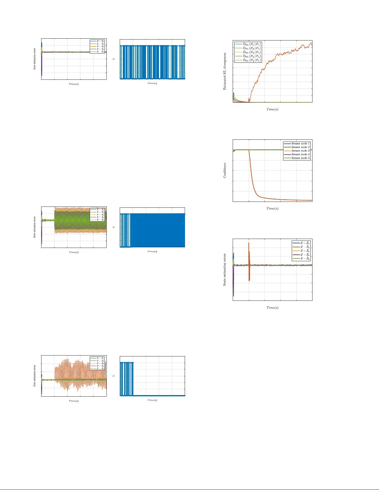
1 This work has been submitted to the IEEE for possible publication. Copyright may be transferred without notice, after which this version may no longer be accessible. Secure Ev ent-T riggered Distrib uted Kalman Filters for State Estimation o v er W ireless Sensor Netw orks Aquib Mustafa, Majid Mazouchi, Hamidreza Modares, Senior Member , IEEE Abstract —In this paper , we analyze the adverse effects of cyber -physical attacks as well as mitigate their impacts on the event-trigger ed distributed Kalman ﬁlter (DKF). W e ﬁrst show that although event-trigger ed mechanisms are highly desirable, the attacker can lev erage the event-trigger ed mechanism to cause non-triggering misbehavior which signiﬁcantly harms the network connectivity and its collective observ ability . W e also show that an attacker can mislead the event-trigger ed mechanism to achieve continuous-triggering misbeha vior which not only drains the communication r esources b ut also harms the network’ s performance. An information-theor etic approach is presented next to detect attacks on both sensors and communication chan- nels. In contrast to the existing results, the r estrictive Gaussian assumption on the attack signal’s probability distribution is not r equired. T o mitigate attacks, a meta-Bayesian approach is presented that incorporates the outcome of the attack detection mechanism to perform second-order inference. The pr oposed second-order inference forms conﬁdence and trust v alues about the truthfulness or legitimacy of sensors’ own estimates and those of their neighbors, respecti vely . Each sensor communicates its conﬁdence to its neighbors. Sensors then incorporate the conﬁdence they receive from their neighbors and the trust they formed about their neighbors into their posterior update laws to successfully discard corrupted inf ormation. Finally , the simulation result v alidates the effectiveness of the presented resilient event-triggered DKF . Index T erms —W ireless sensor network, Event-trigger ed DKF , Attack analysis, Resilient estimation. I . I N T R O D U C T I O N Cyber-physical systems (CPSs) refer to a class of engineer- ing systems that integrate the cyber aspects of computation and communication with physical entities [1]. Integrating communication and computation with sensing and control elements has made CPSs a ke y enabler in designing emerging autonomous and smart systems with the promise of bringing unprecedented beneﬁts to humanity . CPSs have already had a profound impact on v ariety of engineering sectors, includ- ing, process industries [2], robotics [3], smart grids [4], and intelligent transportation [5], health care system [6], to name a fe w . Despite their advantages with vast growth and success, these systems are vulnerable to cyber -physical threats and Aquib Mustafa, Majid Mazouchi and Hamidreza Modares are with the Department of Mechanical Engineering, Michigan State Univ ersity , East Lansing, MI, 48863, USA (e-mails: mustaf15@msu.edu; mazouchi@msu.edu; modaresh@msu.edu). can face fatal consequences if not empo wered with resiliency . The importance of designing resilient and secure CPSs can be witnessed from sev ere damages made by recently reported cyber -physical attacks [7]. A. Related W ork W ireless sensor networks (WSNs) are a class of CPSs for which a set of sensors are spatially distributed to monitor and estimate a variable of interest (e.g., location of a mo ving target, state of a large-scale system, etc.), and hav e various applications such as surveillance and monitoring, target track- ing, and activ e health monitoring [8]. In centralized WSNs, all sensors broadcast their measurements to a center at which the information is fused to estimate the state [9], [10]. These ap- proaches, ho we ver , are communication demanding and prone to single-point-of-failure. T o estimate the state with reduced communication b urden, a distrib uted Kalman ﬁlter (DKF) is presented in [11]-[17], in which sensors exchange their infor- mation only with their neighbors, not with all agents in the network or a central agent. Cost constraints on sensor nodes in a WSN result in corresponding constraints on resources such as energy and communications bandwidth. Sensor nodes in a WSN usually carry limited, irreplaceable energy resources and lifetime adequacy is a signiﬁcant restriction of almost all WSNs. Therefore, it is of vital importance to design ev ent- triggered DKF to reduce the communication burden which consequently improves energy ef ﬁciency . T o this end, se veral energy-ef ﬁcient ev ent-triggered distributed state estimation ap- proaches are presented for which sensor nodes intermittently exchange information [18]-[21]. Moreo ver , the importance of ev ent-triggered state estimation problem is also reported for sev eral practical applications such as smart grids and robotics [22]-[24]. Although event-triggered distributed state estimation is resource-efﬁcient, it provides an opportunity for an attacker to harm the network performance and its connectivity by corrupting the information that is exchanged among sensors, as well as to mislead the ev ent-triggered mechanism. Thus, it is of vital importance to design a resilient e vent-triggered distributed state estimation approach that can perform accurate state estimation despite attacks. In recent years, secure estimation and secure control of CPSs ha ve receiv ed signiﬁcant attention and remarkable results 2 hav e been reported for mitigation of cyber-physical attacks, including denial of service (DoS) attacks [25]-[27], false data injection attacks [28]-[32], and bias injection attacks [33]. For the time-triggered distrib uted scenario, se veral secure state estimation approaches are presented in [34]-[41]. Speciﬁcally , in [34]-[42] authors presented a distributed estimator that allows agents to perform parameter estimation in the pres- ence of attack by discarding information from the adversarial agents. Byzantine-resilient distributed estimator with deter- ministic process dynamics is discussed in [36]. Then, the same authors solved the resilient distributed estimation problem with communication losses and intermittent measurements in [37]. Attack analysis and detection for distributed Kalman ﬁlters are discussed in [38]. Resilient state estimation subject to DoS attacks for power system and robotics applications is pre- sented in [39]-[41]. Although meritable, these aforementioned results for the time-triggered resilient state estimation are not applicable to ev ent-triggered distributed state estimation prob- lems. Recently , authors in [26] addressed the event-triggered distributed state estimation under DoS attacks by employing the co variance intersection fusion approach. Although elegant, the presented approach is not applicable to mitigating the effect of deception attacks. T o our knowledge, resilient state estimation for e vent-triggered DKF under deception attacks is not considered in the literature. For the ﬁrst time, this work not only detects and mitigate the effect of attacks on sensor and communication channel b ut also presents a mathematical analysis for different triggering misbehaviors. B. Contributions and outline This paper contrib utes to analysis, detection, and mitig ation of attacks on event-triggered DKF . T o our knowledge, it is the ﬁrst paper to rigorously analyze how an attacker can lev erage the event- triggering mechanism to harm the state estimation process over WSNs. It also proposes a nov el detection mechanism for detecting attacks on e vent-triggered DKF that does not require the restrictive Gaussian assumption on the probability density function of the attack signal. T o provide mitigation scheme and discard corrupted information, ﬁnally , a novel meta-Bayesian mechanism is developed that performs second-order inference to form conﬁdence and trust about the truthfulness or legitimacy of the outcome of its own ﬁrst-order inference and those of its neighbors, respectiv ely . The details of these contributions are presented as follows: • Attack analysis: It is shown that the attacker can cause emerging non-triggering misbehavior so that the com- promised sensors do not broadcast any information to their neighbors. This can signiﬁcantly harm the network connectivity and its collecti ve observability , which is the necessary condition for solving the distributed state estimation problem. It is also shown that an attacker can achiev e continuous-triggering misbehavior which drains the communication resources. • Attack detections: T o detect adversarial intrusions a Kullback-Leibler (KL) div ergence based detector is pre- sented and estimated via k-nearest neighbors approach to obviate the restrictive Gaussian assumption on the probability density function of the attack signal. • Attack mitigation: T o mitigate attacks on ev ent-triggered DKF and discard corrupted information, a meta-Bayesian approach is employed that performs second-order infer- ence to form conﬁdence and trust about the truthfulness or legitimac y of the outcome of its o wn ﬁrst-order infer- ence (i.e., the posterior belief about the state estimate) and those of its neighbors, respectiv ely . Each sensor communicates its conﬁdence to its neighbors and also incorporates the trust about its neighbors into its posterior update law to put less weight on untrusted data and thus successfully discard corrupted information. Outline: The paper is organized as follows. Section II outlines the preliminary background for the ev ent-triggered DKF . Section III formulates the effect of attacks on the event- triggered DKF and analyzes triggering misbehaviors for it. Attack detection mechanism and conﬁdence-trust based secure ev ent-triggered DKF are presented in Section IV and V , respec- tiv ely . The simulation veriﬁcations are provided in Section VI. Finally , concluding remarks are presented in Section VII. I I . N O T A T I O N S A N D P R E L I M I NA R I E S A. Notations The data communication among sensors in a WSN is captured by an undirected graph G , consists of a pair ( V , E ) , where V = { 1 , 2 , . . . , N } is the set of nodes or sensors and E ⊂ V × V is the set of edges. An edge from node j to node i , represented by ( j , i ) , implies that node j can broadcast information to node i . Moreover , N i = { j : ( j , i ) ∈ E } is the set of neighbors of node i on the graph G . An induced subgraph G w is obtained by remo ving a set of nodes W ⊂ V from the original graph G , which is represented by nodes set V \ W and contains the edges of E with both endpoints in V \ W . Throughout this paper, R and N represent the sets of real numbers and natural numbers, respectively . A T denotes transpose of a matrix A . t r ( A ) and max ( a i ) represent trace of a matrix A and maximum value in the set, respectively . C ( S ) represents the cardinality of a set S. σ max ( A ) , λ max ( A ) , and I n represent maximum singular value, maximum eigen value of matrix A, and an identity matrix of dimension n , respectively . U ( a , b ) with a < b denotes an uniform distribution between the interv al a and b . Consider p X ( x ) as the probability density of the random variable or v ector x with X taking values in the ﬁnite set { 0 , ..., p } . When a random variable X is distributed normally with mean ν and variance σ 2 , we use the notation X ∼ N ( υ , σ 2 ) . E [ X ] and Σ X = E [( X − E [ X ])( X − E [ X ]) T ] denotes, respecti vely , the expectation and the cov ariance of X . Finally , E [ . | . ] represents the conditional expectation. B. Process Dynamics and Sensor Models Consider a process that evolv es according to the following dynamics x ( k + 1 ) = Ax ( k ) + w ( k ) , (1) where A denotes the process dynamic matrix, and x ( k ) ∈ R n and w ( k ) are, respecti vely , the process state and process noise at the time k . The process noise w ( k ) is assumed to be independent and identically distributed (i.i.d.) with Gaussian distribution, and x 0 ∈ N ( ˆ x 0 , P 0 ) represents the initial process state with ˆ x 0 as mean and P 0 as cov ariance, respectively . 3 The goal is to estimate the state x ( k ) for the process (1) in a distributed f ashion using N sensor nodes that communicate through the graph G , and their sensing models are giv en by y i ( k ) = C i x i ( k ) + v i ( k ) ; ∀ i = 1 , · · · , N , (2) where y i ( k ) ∈ R p represents the measurement data with v i ( k ) as the i.i.d. Gaussian measurement noise and C i as the obser- vation matrix of the sensor i , respecti vely . Assumption 1 . The process noise w ( k ) , the measurement noise v i ( k ) , and the initial state x 0 are uncorrelated random vector sequences. Assumption 2 . The sequences w ( k ) and v i ( k ) are zero-mean Gaussian noise with E [ w ( k )( w ( h )) T ] = µ kh Q and E [ v i ( k )( v i ( h )) T ] = µ kh R i , with µ kh = 0 if k 6 = h , and µ kh = 1 otherwise. Moreov er , Q ≥ 0 and R i > 0 denote the noise covariance matrices for process and measurement noise, respecti vely and both are ﬁnite. Deﬁnition 1. (Collecti vely observable) [16]. W e call the plant dynamics (1) and the measurement equation (2) collectiv ely observable, if the pair ( A , C S ) is observable where C s is the stack column vectors of C j , ∀ j ∈ S with S ⊆ V and C ( S ) > N / 2. Assumption 3. The plant dynamics (1) and the measurement equation (2) are collectiv ely observable, but not necessarily locally observable, i.e., ( A , C i ) ∀ i ∈ V is not necessarily observable. Assumptions 1 and 2 are standard assumptions in Kalman ﬁlters. Assumption 3 states that the state of the target in (1) cannot be observed by measurements of any single sensor, i.e., the pairs ( A , C i ) cannot be observable (see for instances [16] and [42]). It also provides the necessary assumption of collectiv ely observ able for the estimation problem to be solv- able. Also note that under Assumption 2, i.e., the process and measurement co variance are ﬁnite, the stochastic observ ability rank condition coincides with the deterministic observ ability [Theorem 1, 43]. Therefore, deterministic observability rank condition holds true irrespecti ve of the process and measure- ment noise. C. Overview of Event-trigg er ed Distributed Kalman F ilter This subsection presents the ov ervie w of the e vent-triggered DKF for estimating the process state x ( k ) in (1) from a collection of noisy measurements y i ( k ) in (2). Let the prior and posterior estimates of the target state x ( k ) for sensor node i at time k be denoted by x i ( k | k − 1 ) and x i ( k | k ) , respectiv ely . In the centralized Kalman ﬁlter, a recursiv e rule based on Bayesian inference is employed to compute the posterior estimate x i ( k | k ) based on its prior estimate x i ( k | k − 1 ) and the new measurement y i ( k ) . When the ne xt measurement comes, the previous posterior estimate is used as a new prior and it proceeds with the same recursi ve estimation rule. In the ev ent-triggered DKF , the recursion rule for computing the posterior incorporates not only its own prior and observ ations, but also its neighbors’ predicti ve state estimate. Sensor i communicates its prior state estimate to its neighbors and if the norm of the error between the actual output and the predictive output becomes greater than a threshold after a ne w observ ation arri ves. That is, it employs the follo wing ev ent-triggered mechanism for e xchange of data with its neighbors k y i ( k ) − C i ˜ x i ( k − 1 ) k < α , (3) where α denotes a predeﬁned threshold for ev ent-triggering. Moreov er , ˜ x i ( k ) denotes the predictive state estimate for sensor i and follows the update la w ˜ x i ( k ) = ζ i ( k ) x i ( k | k − 1 ) + ( 1 − ζ i ( k )) A ˜ x i ( k − 1 ) , ∀ i ∈ V , (4) with ζ i ( k ) ∈ { 0 , 1 } as the transmit function. Note that the predictiv e state estimate update equation in (4) depends on the value of the transmit function ζ i ( k ) which is either zero or one depending on the triggering condition in (3). When ζ i ( k ) = 1, then the prior and predictive state estimates are the same, i.e., ˜ x i ( k ) = x i ( k | k − 1 ) . When ζ i ( k ) = 0 , howe ver , the predictiv e state estimate depends on its own previous state estimate, i.e., ˜ x i ( k ) = A ˜ x i ( k − 1 ) . Incorporating (4), the following recursion rule is used to update the posterior state estimate in the e vent-triggered DKF [18], [20] for sensor i as x i ( k | k ) = x i ( k | k − 1 ) + K i ( k )( y i ( k ) − C i x i ( k | k − 1 )) + γ i ∑ j ∈ N i ( ˜ x j ( k ) − ˜ x i ( k )) , (5) where x i ( k | k − 1 ) = Ax i ( k − 1 | k − 1 ) , (6) is the prior update. Moreover , the second and the third terms in (5) denote, respecti vely , the inno vation part (i.e., the estimation error based on the sensor i t h new observation and its prior prediction) and the consensus part (i.e., deviation of the sensor state estimates from its neighbor’ s state estimates). W e call this recursion rule as the Bayesian ﬁrst-or der inference on the posterior , which provides the belief o ver the value of the state. Moreov er , K i ( k ) and γ i in (5), respectiv ely , denote the Kalman gain and the coupling coefﬁcient. The Kalman gain K i ( k ) in (5) depends on the estimation error covariance ma- trices associated with the prior x i ( k | k − 1 ) and the posterior x i ( k | k ) for the sensor i . Let deﬁne the prior and posterior estimated error covariances as P i ( k | k − 1 ) = E [( x ( k ) − x i ( k | k − 1 ))( x ( k ) − x i ( k | k − 1 )) T ] , P i ( k | k ) = E [( x ( k ) − x i ( k | k ))( x ( k ) − x i ( k | k )) T ] . (7) which are simpliﬁed as [18], [20] P i ( k | k ) = M i ( k ) P i ( k | k − 1 )( M i ( k )) T + K i ( k ) R i ( K i ( k )) T , (8) and P i ( k | k − 1 ) = AP i ( k − 1 | k − 1 ) A T + Q . (9) with M i ( k ) = I n − K i ( k ) C i . Then, the Kalman gain K i ( k ) is designed to minimize the estimation covariance and is gi ven by [18], [20] K i ( k ) = P i ( k | k − 1 )( C i ) T ( R i ( k ) + C i P i ( k | k − 1 )( C i ) T ) − 1 . (10) Let the innov ation sequence r i ( k ) for the node i be deﬁned as r i ( k ) = y i ( k ) − C i x i ( k | k − 1 ) , (11) 4 where r i ( k ) ∼ N ( 0 , Ω i ( k )) with Ω i ( k ) = E [ r i ( k )( r i ( k )) T ] = C i P i ( k | k − 1 ) C i T + R i ( k ) . Note that for the notional simplicity , henceforth we denote the prior and posterior state estimations as x i ( k | k − 1 ) ∆ = ¯ x i ( k ) and x i ( k | k ) ∆ = ˆ x i ( k ) , respectiv ely . Also, the prior cov ariance and the posterior cov ariance are, respectively , denoted by P i ( k | k − 1 ) ∆ = ¯ P i ( k ) and P i ( k | k ) ∆ = ˆ P i ( k ) . Based on equations (6)-(10), the ev ent-triggered DKF algo- rithm becomes T ime updates:  ¯ x i ( k + 1 ) = A ˆ x i ( k ) ( a ) ¯ P i ( k + 1 ) = A ˆ P i ( k ) A T + Q ( k ) ( b ) (12) Measurment updates:            ˆ x i ( k ) = ¯ x i ( k ) + K i ( k )( y i ( k ) − C i ¯ x i ( k )) + γ i ∑ j ∈ N i ( ˜ x j ( k ) − ˜ x i ( k )) , ( a ) ˜ x i ( k ) = ζ i ( k ) ¯ x i ( k ) + ( 1 − ζ i ( k )) A ˜ x i ( k − 1 ) , ( b ) K i ( k ) = ¯ P i ( k ) C T i ( R i ( k ) + C i ¯ P i ( k ) C T i ) − 1 , ( c ) ˆ P i ( k ) = M i ¯ P i ( k ) M i T + K i ( k ) R i ( k )( K i ( k )) T . ( d ) (13) Remark 1. Based on the result presented in [17, Th.1], the ev ent triggered DKF (12)-(13) ensures that the estimation error ˆ x i ( k ) − x ( k ) is e xponentially bounded in the mean square sense ∀ i ∈ V . Remark 2. The consensus gain γ i in (5) is designed such that the stability of the ev ent-triggered DKF in (13)-(14) is guaranteed. Speciﬁcally , as shown in [Theorem 2, 19], if γ i = 2 ( I − K i C i )( Γ i ) − 1 λ max ( L ) λ max (( Γ ) − 1 ) where L denotes the Laplacian matrix associated with the graph G and Γ = d iag { Γ 1 , .., Γ N } with Γ i = ( I − K i C i ) T A T ( ¯ P i ) + A ( I − K i C i ) , ∀ i = { 1 , ..., N } , then the stability of the event-triggered DKF in (13)-(14) is guaranteed. Ho we ver , the design of ev ent-triggered DKF itself is not the concern of this paper and this paper mainly analyzes the adverse effects of cyber-physical attacks on the ev ent-triggered DKF and proposes an information-theoretic approach based attack detection and mitigation mechanism. Note that the presented attack analysis and mitigation can be extended to other ev ent-triggered methods such as [19] and [21] as well. D. Attack Modeling In this subsection, we model the effects of attacks on the ev ent-triggered DKF . An attacker can design a false data injection attack to affect the triggering mechanism presented in (3) and consequently compromise the system beha vior . Deﬁnition 2. (Compromised and intact sensor node). W e call a sensor node that is directly under attack as a compro- mised sensor node. A sensor node is called intact if it is not compromised. Throughout the paper, V c and V \ V c denote, respectiv ely , the set of compromised and intact sensor nodes. Consider the sensing model (2) for sensor node i under the effect of the attack as y a i ( k ) = y i ( k ) + f i ( k ) = C i x i ( k ) + v i ( k ) + f i ( k ) , (14) where y i ( k ) and y a i ( k ) are, respectively , the sensor i ’ s actual and corrupted measurements and f i ( k ) ∈ R p represents the adversarial input on sensor node i . For a compromised sensor node i , let p 0 ⊆ p be the subset of measurements disrupted by the attacker . Let the false data injection attack ¯ f j ( k ) on the communica- tion link be gi ven by ¯ x a j ( k ) = ¯ x j ( k ) + ¯ f j ( k ) , ∀ j ∈ N i . (15) Using (14)-(15), in the presence of an attack on sensor node i and/or its neighbors, its state estimate equations in (13)-(12) becomes        ˆ x a i ( k ) = ¯ x a i ( k ) + K a i ( k )( y i ( k ) − C i ¯ x a i ( k )) + γ i ∑ j ∈ N i ( ˜ x j ( k ) − ˜ x a i ( k )) + f a i ( k ) , ¯ x a i ( k + 1 ) = A ˆ x a i ( k ) , ˜ x a i ( k ) = ζ i ( k ) ¯ x a i ( k ) + ( 1 − ζ i ( k )) A ˜ x a i ( k − 1 ) , (16) where f a i ( k ) = K a i ( k ) f i ( k ) + γ i ∑ j ∈ N i ˜ f j ( k ) , (17) with ˜ f j ( k ) = ζ j ( k ) ¯ f j ( k ) + ( 1 − ζ j ( k )) ˜ f j ( k − 1 ) . The Kalman gain K a i ( k ) in presence of attack is gi ven by K a i ( k ) = ¯ P a i ( k ) C T i ( R i ( k ) + C i ¯ P a i ( k ) C T i ) − 1 . (18) The ﬁrst part in (17) represents the direct attack on sensor node i and the second part denotes the aggregati ve effect of adversarial input on neighboring sensors, i.e., j ∈ N i . Moreov er , ˆ x a i ( k ) , ¯ x a i ( k ) , and ˜ x a i ( k ) denote, respectively , the corrupted posterior , prior , and predicti ve state estimates. The Kalman gain K a i ( k ) depends on the following corrupted prior state estimation error co variance ¯ P a i ( k + 1 ) = A ˆ P a i ( k ) A T + Q . (19) where the corrupted posterior state estimation error cov ariance ˆ P a i ( k ) e v olution is sho wn in the follo wing theorem. Theorem 1. Consider the pr ocess dynamics (1) with compr o- mised sensor model (14) . Let the state estimation equation be given by (16) in the pr esence of attacks modeled by f a i ( k ) in (17) . Then, the corrupted posterior state estimation err or covariance ˆ P a i ( k ) is given by ˆ P a i ( k ) = M a i ( k ) ¯ P a i ( k )( M a i ( k )) T + K a i ( k )[ R i ( k ) + Σ f i ( k )]( K a i ( k )) T + 2 γ i ∑ j ∈ N i ( _ P a i , j ( k ) − _ P a i ( k ))( M a i ( k )) T − 2 K a i ( k ) Ξ f ( k ) + γ i 2 ( ∑ j ∈ N i ( ˜ P a j ( k ) − 2 ˜ P a i , j ( k ) + ˜ P a i ( k )) , (20) wher e Σ f i ( k ) and Ξ f ( k ) denote the attac ker’ s input dependent covariance matrices and M a i = ( I n − K a i ( k ) C i ) with K a i ( k ) as the Kalman gain and ¯ P a i ( k ) as the prior state estimation err or covariance update in (18) and (19) , respectively . Moreo ver , ˜ P a i , j ( k ) and _ P a i , j ( k ) ar e cr oss-corr elated estimation err or co- variances updated according to (73) - (75) . Pr oof. See Appendix A. Note that the corrupted state estimation error cov ariance recursion ˆ P a i ( k ) in (20) depends on the attacker’ s input dis- tribution. Since the state estimation depends on compromised estimation error co variance ˆ P a i ( k ) , therefore, the attacker can design its attack signal to blow up the estimates of the desired process state and damage the system performance. 5 I I I . E FF E C T O F A T T AC K O N T R I G G E R I N G M E C H A N I S M This section presents the effects of cyber -physical attacks on the event-triggered DKF . W e show that although event- triggered approaches are energy efﬁcient, they are prone to triggering misbehaviors, which can harm the network connec- tivity , observability and drain its limited resources. A. Non-triggering Misbehavior In this subsection, we sho w ho w an attacker can manipulate the sensor measurement to mislead the e vent-triggered mecha- nism and damage network connectivity and collecti ve observ- ability by causing non-triggering misbehavior as deﬁned in the following Deﬁnition 3. Deﬁnition 3 ( Non-triggering Misbehavior). The attacker designs an attack strategy such that a compromised sensor node does not transmit any information to its neighbors by misleading the triggering mechanism in (3), ev en if the actual performance deviates from the desired one. The following theorem shows how a false data injection attack, followed by an eavesdropping attack, can manipulate the sensor reading to a void the e vent-triggered mechanism (3) from being violated while the actual performance could be far from the desired one. T o this end, we ﬁrst deﬁne the vertex cut of the graph as follows. Deﬁnition 4 (V ertex cut). A set of nodes C ⊂ V is a v ertex cut of a graph G if removing the nodes in the set C results in disconnected graph clusters. Theorem 2. Consider the process dynamics (1) with N sensor nodes (2) communicating over the graph G . Let sensor i be under a false data injection attack given by y a i ( k ) = y i ( k ) + θ a i ( k ) 1 p , ∀ k ≥ L + 1 , (21) wher e y i ( k ) is the actual sensor measur ement at time instant k and L denotes the last triggering time instant. Mor eover , θ a i ( k ) ∼ U ( a ( k ) , b ( k )) is a scalar uniformly distributed ran- dom variable in the interval ( a ( k ) , b ( k )) with  a ( k ) = ϕ − k C i ˜ x i ( k − 1 ) k + k y i ( k ) k , b ( k ) = ϕ + k C i ˜ x i ( k − 1 ) k − k y i ( k ) k , (22) wher e ˜ x i ( k ) and ϕ < α denote, r espectively , the pr edictive state estimate and an arbitr ary scalar value less than the trigg ering thr eshold α . Then, 1) The triggering condition (3) will not be violated for the sensor node i and it shows non-triggering misbehavior; 2) The original graph G is clustered into several sub- graphs, if all sensors in a vertex cut ar e under attack (21) . Pr oof. T aking norms from both sides of (21), the corrupted sensor measurement y a i ( k ) becomes k y a i ( k ) k =   y i ( k ) + θ a i ( k ) 1 p   . (23) Using the triangular inequality for (23) yields k y i ( k ) k −   θ a i ( k ) 1 p   ≤ k y a i ( k ) k ≤ k y i ( k ) k +   θ a i ( k ) 1 p   . (24) Based on the bounds of θ a i ( k ) , gi ven by (22), (24) becomes k C i ˜ x i ( k − 1 ) k − ϕ ≤ k y a i ( k ) k ≤ k C i ˜ x i ( k − 1 ) k + ϕ , which yields ( k y a i ( k ) k − k C i ˜ x i ( k − 1 ) k − ϕ )( k y a i ( k ) k − k C i ˜ x i ( k − 1 ) k + ϕ ) ≤ 0 . This implies that the condition k y a i ( k ) − C i ˜ x i ( k − 1 ) k ≤ ϕ < α , always holds true. Therefore, under (21)-(22), the corrupted sensor node i sho ws non-triggering misbehavior , which prov es part 1. W e now prove part 2. Let A n ⊆ V c be the set of sensor nodes showing non-triggering misbehavior . Then, based on the presented result in part 1, under the attack signal (21), sensor nodes in the set A n are misled by the attack er and consequently do not transmit an y information to their neighbors which make them to act as sink nodes. Since the set of sensor nodes A n is assumed to be a verte x cut. Then, the non-triggering misbehavior of sensor nodes in A n prev ents information ﬂow from one portion of the graph G to another portion of the graph G and thus clusters the original graph G into subgraphs. This completes the proof. Remark 3. Note that to design the presented strategic false data injection attack signal gi ven in (21) an attacker needs to eav esdrop the actual sensor measurement y i ( k ) and the last transmitted prior state estimate ¯ x i ( L ) through the communica- tion channel. The attacker then determines the predicti ve state estimate ˜ x i ( k ) using the dynamics in (5) at each time instant k ≥ L + 1 to achiev e non-triggering misbehavior for the sensor node i . W e pro vide Example 1 for further illustration of the results of Theorem 2. Figure 1: Effect of non-triggering misbehavior on sensor nodes { 5,6 } cluster the graph G in the two isolated graphs G 1 and G 2 . Example 1. Consider a graph topology for a distributed sensor network gi ven in ﬁg. 1. Let the vertex cut A n = { 5 , 6 } be under the presented false data injection attack in Theorem 2 and show non-triggering misbehavior . Then, the sensor nodes in A n = { 5 , 6 } do not transmit an y information to their neighbors under the designed false data injection attack. Moreover , the sensor nodes in A n = { 5 , 6 } act as sink nodes and prevent information ﬂow from subgraph G 1 to subgraph G 2 which clusters the graph G into two non-interacting subgraphs G 1 and G 2 as sho wn in Fig. 1. This example sho ws that the attacker 6 can compromise the v ertex cut A n of the original graph G such that it sho ws non-triggering misbehavior and harm the network connectivity or cluster the graph into various non-interacting subgraphs. W e now analyze the effect of non-triggering misbehavior on the collecti ve observ ability of the sensor network. T o do so the following deﬁnitions are needed. Deﬁnition 5 (Potential Set). A set of nodes P ⊂ V is said to be a potential set of the graph G if the pair ( A , C V \ P ) is not collectiv ely observable. Deﬁnition 6 (Minimal Potential Set). A set of nodes P m ⊂ V is said to be a minimal potential set if P m is a potential set and no subset of P m is a potential set. Remark 4. Note that if the attacker kno ws the graph structure and the local pair ( A , C i ) , ∀ i ∈ V . Then, the attacker can identify the minimum potential set of sensor nodes P m in the graph G and achie ves non-triggering misbehavior for P m . Thus, the set of sensor nodes P m does not exchange any information with its neighbors and becomes isolated in the graph G . Corollary 1. Let the set of sensors that shows non-triggering misbehavior be the minimal potential set S n . Then, the network is no long er collectively observable and the pr ocess state r econstruction fr om the distributed sensor measur ements is impossible. Pr oof. According to the statement of the corollary , S n repre- sents a minimal potential set of the graph G and sho ws non- triggering misbeha vior . Then, the sensor nodes in the set S n do not transmit any information to their neighbors and they act as sink nodes, i.e., they only absorb information. Therefore, the exchange of information happen just between the remaining sensor nodes in the graph G \ S n . Hence, after e xcluding the minimum potential nodes S n , the pair ( A , C G \ S n ) becomes unobservable based on the Deﬁnitions 5 and 6, and thus makes the state reconstruction impossible. This completes the proof. B. Continuous-triggering Misbehavior In this subsection, we discuss how an attacker can com- promise the actual sensor measurement to mislead the event- triggered mechanism and achie ves continuous-triggering mis- behavior and thus results in a time-driv en DKF that not only drains the communication resources but also continuously propagates the adverse effect of attack in the network. Deﬁnition 7 (Continuous-triggering Misbehavior). Let the attacker design an attack strategy such that it deceiv es the triggering mechanism in (3) at each time instant. This turns the ev ent-dri ven DKF into a time-driven DKF that continuously exchanges corrupted information among sensor nodes. W e call this a continuous-triggering misbeha vior . W e now sho w how a reply attack, followed by an eaves- dropping attack, can manipulate the sensor reading to cause continuous violation of the e vent-triggered mechanism (3). Theorem 3. Consider the process dynamics (1) with N sensor nodes (2) communicating over the graph G . Let the sensor node i in (2) be under a r eplay attack given by y a i ( k ) = C i ¯ x i ( k − 1 ) + υ i ( k ) , ∀ k ≥ l + 1 , (25) wher e ¯ x i ( k − 1 ) repr esents the last transmitted prior state and υ i ( k ) denotes a scalar disruption signal. l denotes the last triggering time instant when intact prior state estimate was transmitted. Then, the sensor node i shows continuous- triggering misbehavior if the attac ker selects k υ i ( k ) k > α . Pr oof. T o mislead a sensor to cause a continuous-triggering misbehavior , the attacker needs to design the attack signal such that the ev ent-triggered condition (3) is constantly being violated, i.e., k y a i ( k ) − C i ˜ x i ( k − 1 ) k ≥ α all the time. The attacker can ea vesdrop the last transmitted prior state estimate ¯ x i ( k − 1 ) and design the strategic attack signal gi ven by (25). Then, one has y a i ( k ) − C i ˜ x i ( k − 1 ) = C i ¯ x i ( k − 1 ) + δ i ( k ) − C i ˜ x i ( k − 1 ) = C i ¯ x i ( k − 1 ) + υ i ( k ) − C i [ ζ i ( k − 1 ) ¯ x i ( k − 1 ) +( 1 − ζ i ( k − 1 )) A ¯ x i ( k − 2 )] = ( 1 − ζ i ( k − 1 )) C i [ ¯ x i ( k − 1 ) − A ¯ x i ( k − 2 )] + υ i ( k ) , (26) T aking the norm from both sides of (26) yields k y a i ( k ) − C i ˜ x i ( k − 1 ) k = k ( 1 − ζ i ( k − 1 )) C i [ ¯ x i ( k − 1 ) − A ¯ x i ( k − 2 )] + υ i ( k ) k , (27) Since for k = l + 1, ζ i ( l ) = 1 k y a i ( l + 1 ) − C i ˜ x i ( l ) k = k υ i ( l + 1 ) k , (28) If the attacker selects υ i ( l + 1 ) in (28) such that k υ i ( l + 1 ) k > α , then the attack signal (25) ensures triggering at time instant k = l + 1 . Then, based on similar ar gument for (27), ∀ k ≥ l + 1 k y a i ( k ) − C i ˜ x i ( k − 1 ) k = k υ i ( k ) k > α , which ensures continuous triggering misbehavior . This com- pletes the proof. T o achieve continuous-triggering misbehavior the attacker needs to eavesdrop prior state estimates ¯ x i ( k − 1 ) at each triggering instant and selects the υ i ( k ) large enough such that k υ i ( k ) k > α always holds true. Note that continuous-triggering misbehavior can completely ruin the adv antage of ev ent-triggered mechanisms and turn it into time-dri ven mechanisms. This signiﬁcantly increases the communication burden. Since nodes in the WSNs are usually powered through batteries with limited ener gy , the attacker can drain sensors limited resources by designing the above- discussed attack signals to achie ve continuous-triggering mis- behavior , and, consequently can make them non-operating in the network along with the deteriorated performance of the network. Note that although we classiﬁed attacks into non-triggering misbehavior and continuous-triggering misbehavior , to analyze how the attacker can le verage the ev ent-triggered mechanism, the following analysis, detection and mitigation appr oaches are not restricted to any class of attacks. I V . A T TAC K D E T E C T I O N In this section, we present an entropy estimation-based attack detection approach for the ev ent-triggered DKF . 7 The KL diver gence is a non-neg ativ e measure of the relativ e entropy between two probability distributions which is deﬁned as follows. Deﬁnition 8 (KL Divergence) [33] . Let X and Z be two random variables with probability density function P X and P Z , respectiv ely . The KL diver gence measure between P X and P Z is deﬁned as D K L ( P X || P Z ) = Z θ ∈ Θ P X ( θ ) log  P X ( θ ) P Z ( θ )  , (29) with the following properties [43] 1) D K L ( P X || P Z ) ≥ 0; 2) D K L ( P X || P Z ) = 0 if and only if, P X = P z ; 3) D K L ( P X || P Z ) 6 = D K L ( P Z || P X ) . In the existing resilient literature, the entrop y-based anomaly detectors need to know the probability density func- tion of sequences, i.e., P X and P Z , in (29) to determine the relativ e entropy . In most of the cases, authors assume that the probability density function of corrupted innov ation sequence remains Gaussian (see [33] and [44] for instance). Since, the attacker’ s input signal is unkno wn, it is restricti ve to assume that the probability density function of the corrupted sequence remains Gaussian. T o relax this restrictive assumption on probability density function of the corrupted sequence, we estimate the relativ e entropy between two random sequences X and Z using k − near est neighbor ( k − N N ) based div ergence estimator [46]. Let { X 1 , . . . , X n 1 } and { Z 1 , . . . , Z n 2 } be i.i.d. samples dra wn independently from P X and P Z , respectiv ely with X j , Z j ∈ R m . Let d X k ( i ) be the Euclidean distance between X i and its k − N N in { X l } l 6 = i . The k − N N of a sample s in { s 1 , . . . , s n } is s i ( k ) where i ( 1 ) , . . . , i ( n ) such that   s − s i ( 1 )   ≤   s − s i ( 2 )   ≤ . . . ≤   s − s i ( n )   . More speciﬁcally , the Euclidean distance d X k ( i ) is given by [45] d X k ( i ) = min j = 1 ,..., n 1 , j 6 = { i , j 1 ,..., j k − 1 }   X i − X j   The k − N N based relativ e entropy estimator is gi ven by [46] ˆ D K L ( P X || P Z ) = m n 1 n 1 ∑ i = 1 log d Z k ( i ) d X k ( i ) + log n 2 n 1 − 1 . (30) The innovation sequences represent the deviation of the actual output of the system from the estimated one. It is known that innovation sequences approach a steady state quickly and thus it is reasonable to design inno vation-based anomaly detectors to capture the system abnormality [33]. Using the in- nov ation sequence of each sensor and the innov ation sequences that it estimates for its neighbors, we present innovation based div ergence estimator and design detectors to capture the effect of the attacks on the ev ent-triggered DKF . Based on innovation expression (11), in the presence of attack, one can write the compromised innov ation r a i ( k ) for sensor node i with disrupted measurement y a i ( k ) in (14) and state estimation ¯ x a i based on (16) as r a i ( k ) = y a i ( k ) − C i ¯ x a i ( k ) . (31) Let { r a i ( l ) , . . . , r a i ( l − 1 + w ) } and { r i ( l ) , . . . , r i ( l − 1 + w ) } be i.i.d. p -dimensional samples of corrupted and nominal innov ation sequences with probability density function P r a i and P r i , respectively . The nominal innovation sequence follows r i ( k ) deﬁned in (11). Using k − N N based relati ve entropy estimator (30), one has [46] ˆ D K L ( P r a i || P r i ) = p w w ∑ j = 1 log d r i k ( j ) d r a i k ( j ) + log w w − 1 , ∀ i ∈ V . (32) Deﬁne the av erage of the estimated KL di ver gence over a time window of T as Φ i ( k ) = 1 T k ∑ l = k − T + 1 ˆ D K L ( P r a i || P r i ) , ∀ i ∈ V . (33) Now , in the following theorem, it is shown that the effect of attacks on the sensors can be captured using (33). Theorem 4. Consider the distributed sensor network (1) - (2) under attack on sensor . Then, 1) in the absence of attack, Φ i ( k ) = log ( w / w − 1 ) , ∀ k ; 2) in the pr esence of attack, Φ i ( k ) > δ , ∀ k > l a , wher e δ and l a denotes, r espectively , a pr edeﬁned thr eshold and the time instant at which the attack happen. Pr oof. In the absence of attack, the samples of innov ation se- quences { r a i ( l ) , . . . , r a i ( l − 1 + w ) } and { r i ( l ) , . . . , r i ( l − 1 + w ) } are similar . Then, the Euclidean distance d r a i k ( j ) = d r i k ( j ) , ∀ j ∈ { 1 , ..., w } and one has ˆ D K L ( P r a i || P r i ) = log w w − 1 , ∀ i ∈ V . (34) Based on (34), one has Φ i ( k ) = 1 T k ∑ l = k − T + 1 log w w − 1 = log w w − 1 < δ , ∀ i ∈ V . (35) where log ( w / w − 1 ) in (42) depends on the sample size of innovation sequence and log ( w / w − 1 ) ≤ 0 . 1 , ∀ w ≥ 10. Therefore, the predeﬁned threshold δ can be selected with some δ > 0 . 1 such that the condition in (42) is always satisﬁed. This complete the proof of part 1. In the presence of attack, the samples of innovation se- quences { r a i ( l ) , . . . , r a i ( l − 1 + w ) } and { r i ( l ) , . . . , r i ( l − 1 + w ) } are different, i.e., d r a i k ( j ) 6 = d r i k ( j ) , ∀ j ∈ { 1 , ..., w } . More specif- ically , d r i k ( j ) > d r a i k ( j ) , ∀ j ∈ { 1 , ..., w } due to change in the corrupted innovation sequence. Therefore, based on (32) the estimated relativ e entropy between sequences becomes ˆ D K L ( P r a i || P r i ) = p w w ∑ j = 1 log ( 1 + ∆ r i k ( j ) d r a i k ( j ) ) + log w w − 1 , ∀ i ∈ V , (36) with ∆ r i k ( j ) as the change in Euclidean distance due to cor- rupted innov ation sequence. Based on (36), one has ˆ D K L ( P r a i || P r i ) = p w w ∑ j = 1 log ( 1 + ∆ r i k ( j ) d r a i k ( j ) ) + log w w − 1  log w w − 1 . (37) Thus, one has Φ i ( k ) = 1 T k ∑ l = k − T + 1 ˆ D K L ( P r a i || P r i ) > δ , ∀ i ∈ V , (38) where T and δ denote the sliding window size and the predeﬁned design threshold. This completes the proof. 8 Based on Theorem 4, one can use the following condition for attack detection.  Φ i ( k ) < δ : H 0 , Φ i ( k ) > δ : H 1 , (39) where δ denotes the designed threshold for detection, the null hypothesis H 0 represents the intact mode of sensor nodes and H 1 denotes the compromised mode of sensor nodes. Remark 5. Note that in the absence of an attack, the in- nov ation sequence has a known zero-mean Gaussian distri- bution due to the measurement noise. Based on the prior system knowledge, one can alw ays consider that the nominal innov ation sequence is zero-mean Gaussian distribution with predeﬁned co variance. The bound on the predeﬁned cov ariance can be determined during normal operation of the ev ent- triggered DKF . This assumption for the knowledge of the nominal innov ation sequence for attack detection is standard in the existing literature (see [44] for instance). The designed threshold δ in (39) is a predeﬁned parameter and chosen appropriately for the detection of the attack signal. Moreover , the selection of detection threshold based on expert knowledge is standard in the existing literature. For example, sev eral results on adversary detection and stealthiness ha ve considered similar thresholds [33]-[34]. Algorithm 1 Detecting attacks on sensors. 1: Initialize with a time window T and detection threshold δ . 2: procedur e ∀ i = 1 , . . . , N 3: Use samples of innov ation sequences { r a i ( l ) , . . . , r a i ( l − 1 + w ) } and { r i ( l ) , . . . , r i ( l − 1 + w ) } based on (31) and (11), ∀ l ∈ k . 4: Estimate the ˆ D K L ( P r a i || P r i ) using (37). 5: Compute Φ i ( k ) as (38) and use condition in (39) to detect attacks on sensors. 6: end procedur e Based on the results presented in Theorem 4 and Algorithm 1, one can capture attacks on both sensors and communi- cation links, but it cannot identify the speciﬁc compromised communication link as modelled in (15). T o detect the source of attacks, we present an estimated entropy-based detector to capture the ef fect of attacks on the speciﬁc communication channel. More speciﬁcally , the relative entropy between the estimated innov ation sequences for the neighbors at particular sensor node and the nominal innov ation sequence of the considered sensor node is estimated using (30). Deﬁne the estimated innovation sequences ζ a i , j ( k ) for a neighbor j under attacks on communication channel from the sensor node i side as ζ a i , j ( k ) = y i ( k ) − C j ˜ x a j ( k ) , (40) where ˜ x a j ( k ) is the corrupted communicated state estimation of neighbor j at sensor node i at the last triggering instant. Let { ζ a i , j ( l ) , . . . , ζ a i , j ( l − 1 + w ) } be i.i.d. p -dimensional sam- ples of neighbor’ s estimated innov ation at the sensor node i with probability density function P ζ a i , j . Using k − N N based relativ e entropy estimator (30), one has ˆ D K L ( P ζ a i , j || P r i ) = p w w ∑ j = 1 log d r i k ( j ) d ζ a i , j k ( j ) + log w w − 1 , ∀ i ∈ V , j ∈ N i . (41) Note that in the presence of attacks on the communica- tion channels, the neighbor’ s actual innovation differs the neighbor’ s estimated innov ation at sensor i . In the absence of the attack, the mean v alue of all the sensor state estimates con ver ge to the mean of the desired process state at steady state, and, therefore, the innovation sequences r i and ζ a i , j hav e the same zero mean Gaussian distributions. In the presence of attack, howe ver , as shown in Theorem 5 and Algorithm 2, their distributions div erge. Deﬁne the average of the KL div ergence over a time window of T as Ψ i , j ( k ) = 1 T k ∑ l = k − T + 1 ˆ D K L ( P ζ a i , j || P r i ) , ∀ i ∈ V , j ∈ N i . (42) Theorem 5. Consider the distributed sensor network (1) - (2) under attack on communication links (15) . Then, in the pr esence of an attack, Ψ i , j ( k ) > δ , ∀ k where δ denotes a pr edeﬁned thr eshold. Pr oof. The result follows a similar ar gument as giv en in the proof of part 2 of Theorem 4. Algorithm 2 Detecting attack on a speciﬁc communication link. 1: Initialize with a time window T and detection threshold δ . 2: procedur e ∀ i = 1 , . . . , N 3: For each sensor node j ∈ N i , use samples of innov ation sequences { ζ a i , j ( l ) , . . . , ζ a i , j ( l − 1 + w ) } and { r i ( l ) , . . . , r i ( l − 1 + w ) } based on (40) and (11), ∀ l ∈ k . 4: Estimate the ˆ D K L ( P ζ a i , j || P r i ) using (41). 5: Compute Ψ i , j ( k ) as (42) and use same argument in (39) to detect attacks on speciﬁc communication link. 6: end procedur e V . S E C U R E D I S T R I B U T E D E S T I M A T I O N M E C H A N I S M This section presents a meta-Bayesian approach for secure ev ent-triggered DKF , which incorporates the outcome of the attack detection mechanism to perform second-order infer- ence and consequently form beliefs over beliefs. That is, the second-order inference forms conﬁdence and trust about the truthfulness or legitimacy of the sensors’ o wn state estimate (i.e., the posterior belief of the ﬁrst-order Bayesian inference) and those of its neighbor’ s state estimates, respecti vely . Each sensor communicates its conﬁdence to its neighbors. Then sensors incorporate the conﬁdence of their neighbors and their own trust about their neighbors into their posterior update laws to successfully discard the corrupted information. 9 A. Conﬁdence of sensor nodes The second-order inference forms a conﬁdence v alue for each sensor node which determines the le vel of trustworthiness of the sensor about its own measurement and state estimate (i.e., the posterior belief of the ﬁrst-order Bayesian inference). If a sensor node is compromised, then the presented attack detector detects the adversary and it then reduces its level of trustworthiness about its own understanding of the en vi- ronment and communicates it with its neighbors to inform them the signiﬁcance of its outgoing information and thus slow down the attack propagation. T o determine the conﬁdence of the sensor node i , based on the diver gence ˆ D K L ( P r a i || P r i ) from Theorem 4, we ﬁrst deﬁne χ i ( k ) = ϒ 1 ϒ 1 + ˆ D K L ( P r a i || P r i ) , (43) with 0 < ϒ 1 < 1 represents a predeﬁned threshold to account for the channel fading and other uncertainties. Then, in the following lemma, we formally present the results for the conﬁdence of sensor node i . Lemma 1. Let β i ( k ) be the conﬁdence of the sensor node i which is updated using β i ( k ) = k − 1 ∑ l = 0 ( κ 1 ) k − l + 1 χ i ( l ) , (44) wher e χ i ( k ) is deﬁned in (43) , and 0 < κ 1 < 1 is a discount factor . Then, β i ( k ) ∈ ( 0 , 1 ] and 1) β i ( k ) → 0 , ∀ i ∈ V c ; 2) β i ( k ) → 1 , ∀ i ∈ V \ V c . Pr oof. Based on the e xpression (43), since ˆ D K L ( P r a i || P r i ) ≥ 0, one has χ i ( k ) ∈ ( 0 , 1 ] . Then, using (44), one can infer that β i ( k ) ∈ ( 0 , 1 ] . Now according to Theorem 4, if the sensor node i is under attack, then ˆ D K L ( P r a i || P r i ) >> ϒ 1 in (43), which makes χ i ( k ) close to zero. Then, based on expression (44) with the discount factor 0 < κ 1 < 1 , the conﬁdence β i ( k ) in (44) approaches zero, and thus the i t h sensor’ s belief about the trustworthiness of its own information would be low . This completes the proof of part 1. On the other hand, based on Theorem 4, in the absence of attacks, ˆ D K L ( P r a i || P r i ) → 0 as w → ∞ , which makes χ i ( k ) close to one and, consequently , β i ( k ) becomes close to one. This indicates that the i t h sensor node is conﬁdent about its own state estimate. This completes the proof of part 2. Note that the expression for the conﬁdence of sensor node i in (44) can be implemented using the following difference equation β i ( k + 1 ) = β i ( k ) + κ 1 χ i ( k ) . Note also that the discount factor in (44) determines ho w much we value the current experience with regards to past experiences. It also guarantees that if the attack is not per- sistent and disappears after a while, or if a short-period adversary rather than attack (such as packet dropout) causes, the belief will be reco vered, as it mainly depends on the current circumstances. B. T rust of sensor nodes about their incoming information Similar to the previous subsection, the second-order in- ference forms trust of sensor nodes to represent their le vel of trust on their neighboring sensor’ s state estimates. Trust decides the usefulness of the neighboring information in the state estimation of sensor node i . The trust of the sensor node i on its neighboring sensor j can be determined based on the di ver gence ˆ D K L ( P ζ a i , j || P r i ) in (40) from Theorem 5, from which we deﬁne θ i , j ( k ) = Λ 1 Λ 1 + ˆ D K L ( P ζ a i , j || P r i ) , (45) where 0 < Λ 1 < 1 represents a predeﬁned threshold to account for the channel fading and other uncertainties. Then, in the following lemma, we formally present the results for the trust of the sensor node i on its neighboring sensor j . Lemma 2. Let σ i , j ( k ) be the trust of the sensor node i on its neighboring sensor j which is updated using σ i , j ( k ) = k − 1 ∑ l = 0 ( κ 2 ) k − l + 1 θ i , j ( l ) , (46) wher e θ i , j ( k ) is deﬁned in (45) , and 0 < κ 2 < 1 is a discount factor . Then, σ i , j ( k ) ∈ ( 0 , 1 ] and 1) σ i , j ( k ) → 0 , ∀ j ∈ V c ∩ N i ; 2) σ i , j ( k ) → 1 , ∀ j ∈ V \ V c ∩ N i . Pr oof. The result follows a similar ar gument as giv en in the proof of Lemma 1. Note that the trust of sensor node i in (46) can be imple- mented using the follo wing difference equation σ i , j ( k + 1 ) = σ i , j ( k ) + κ 2 θ i , j ( k ) . Using the presented idea of trust, one can identify the attacks on the communication channel and discard the contrib ution of compromised information for the state estimation. C. Attack mitigation mechanism using conﬁdence and trust of sensors This subsection incorporates the conﬁdence and trust of sensors to design a resilient ev ent-triggered DKF . T o this end, using the presented conﬁdence β i ( k ) in (44) and trust σ i , j ( k ) in (46), we design the resilient form of the e vent-triggered DKF as ˆ x i ( k ) = ¯ x i ( k ) + K i ( k )( β i ( k ) y i ( k ) + ( 1 − β i ( k )) C i m i ( k ) − C i ¯ x i ( k )) + γ i ∑ j ∈ N i σ i , j ( k ) β j ( k )( ˜ x j ( k ) − ˜ x i ( k )) , (47) where the weighted neighbor’ s state estimate m i ( k ) is deﬁned as m i ( k ) = 1 | N i | ∑ j ∈ N i σ i , j ( k ) β j ( k ) ˜ x j ( k ) ≈ x ( k ) + ε i ( k ) , ∀ k k ε i ( k ) k < τ , (48) where ε i ( k ) denotes the de viation between the weighted neigh- bor’ s state estimate m i ( k ) and the actual process state x ( k ) . Note that in (48) the weighted state estimate depends on the trust v alues σ i , j ( k ) and the conﬁdence values β j ( k ) , ∀ j ∈ N i . Since the weighted state estimate depends only on the infor- mation from intact neighbors, then one has k ε i ( k ) k < τ for some τ > 0 , ∀ k . F or the sak e of mathematical representation, 10 we approximate the weighted state estimate m i ( k ) in terms of the actual process state x ( k ) , i.e., m i ( k ) ≈ x ( k ) + ε i ( k ) . W e call this a meta-Bayesian inference that integrates the ﬁrst- order inference (state estimates) with second-order estimates or belief (trust and conﬁdence on the trustworthiness of state estimate beliefs). Deﬁne the prior and predicti ve state estimation errors as ¯ η i ( k ) = x ( k ) − ¯ x i ( k ) ˜ η i ( k ) = x ( k ) − ˜ x i ( k ) , (49) Using the threshold in triggering mechanism (3), one has k ˜ η i ( k ) k − k x ( k + 1 ) − x ( k ) + v i ( k + 1 ) k ≤ α / k C i k , k ˜ η i ( k ) k ≤ α / k C i k + B , (50) where B denotes the bound on k x ( k + 1 ) − x ( k ) + v i ( k + 1 ) k . Other notations used in the following theorem are given by ¯ η ( k ) = [ ¯ η 1 ( k ) , . . . , ¯ η N ( k )] , M ( k ) = d iag [ M 1 ( k ) , . . . , M N ( k )] ϒ = d iag [ γ 1 , . . . , γ N ] , ϒ m = k max { γ i } k , ∀ i ∈ V , ¯ β = ( I N − d iag ( β i )) , E ( k ) = [ ε 1 ( k ) , . . . , ε N ( k )] , ˜ η ( k ) = [ ˜ η 1 ( k ) , . . . , ˜ η N ( k )] . (51) Assumption 4. At least ( C ( N i ) / 2 ) + 1 neighbors of the sensor node i are intact. Assumption 4 is similar to the assumption found in the secure estimation and control literature [28], [35]. Necessary and sufﬁcient condition for any centralized or distributed estimator to resiliently estimate actual state is that the number of attacked sensors is less than half of all sensors. Remark 6. Note that the proposed notion of trust and conﬁdence for hybrid attacks on sensor networks for ev ent- triggered DKF can also be seen as the weightage in the cov ariance fusion approach. Although co variance intersection- based Kalman consensus ﬁlters hav e been widely used in the literature to deal with unknown correlations in sensor networks (for instants see [11]-[14] and [39]-[41]), most of these results considered the time-triggered distributed state estimation problem with or without any adversaries. Compared with the existing results, howe ver , a nov elty of this work lies in detecting and mitigating the effect of attacks on sensors and communication channels for e vent-triggered DKF and provid- ing a rigorous mathematical analysis for different triggering misbehaviors. Theorem 6. Consider the r esilient event trigger ed DKF (47) with the trig gering mechanism (3). Let the time-varying gr aph be G ( k ) such that at each time instant k , Assumptions 3 and 4 ar e satisﬁed. Then, 1) The following uniform bound holds on state estimation err or in (49) , despite attac ks k ¯ η ( k ) k ≤ ( A o ) k k ¯ η ( 0 ) k + k − 1 ∑ m = 0 ( A o ) k − m − 1 B o , (52) wher e A o = σ max (( I N ⊗ A ) M ( k )) , B o = σ max ( A ) σ max ( L ( k )) ϒ m p N ( α / k C i k + B ) +( σ max ( A ) + σ max ( A o ))   ¯ β   √ N τ , (53) with L ( k ) denotes the conﬁdence and trust dependent time-varying graph Laplacian matrix, and bound τ deﬁned in (48) ; 2) The uniform bound on the state estimation err or (52) becomes lim k → ∞ k ¯ η ( k ) k ≤ A o B o 1 − A o . (54) Mor eover , other notations used in (53) ar e deﬁned in (51) . Pr oof. Using the presented resilient estimator (47), one has ¯ x i ( k + 1 ) = A ˆ x i ( k ) = A ( ¯ x i ( k ) + K i ( k )( β i ( k ) y i ( k ) + ( 1 − β i ( k )) C i m i ( k ) − C i ¯ x i ( k )) + γ i ∑ j ∈ N i σ i , j ( k ) β j ( k )( ˜ x j ( k ) − ˜ x i ( k ))) , (55) Substituting (48) into (55) and using (49), the state estimation error dynamics becomes ¯ η i ( k + 1 ) = AM i ( k ) ¯ η i ( k ) + A γ i ∑ j ∈ N i a i j ( k )( ˜ η j ( k ) − ˜ η i ( k )) − AK i ( k )( 1 − β i ( k )) C i ε i ( k ) , (56) where a i j ( k ) = σ i , j ( k ) β j ( k ) and M i ( k ) = I − K i ( k ) C i . Using (56) and notations deﬁned in (51), the global form of error dynamics becomes ¯ η ( k + 1 ) = ( I N ⊗ A ) M ( k ) ¯ η ( k ) − ( ϒ ⊗ A ) L ( k ) ˜ η ( k ) − ( ¯ β ⊗ A )( I nN − M ( k )) E ( k )) . (57) Note that Assumption 4 implies that the total number of the compromised sensors is less than half of the total number of sensors in the network. That is, if q neighbors of an intact sensor node are attacked and collude to send the same value to mislead it, there still exists q + 1 intact neighbors that communicate values different from the compromised ones. Moreov er , since at least half of the intact sensor’ s neighbors are intact, it can update its beliefs to discard the compro- mised neighbor’ s state estimates. Furthermore, since the time- varying graph G ( k ) resulting from isolating the compromised sensors, based on Assumptions 3 and 4, the entire network is still collecti vely observable. Using the trust and conﬁdence of neighboring sensors, the incoming information from the compromised communication channels is discarded. Now taking norm of equation (57) from both sides and then using the triangular inequality , one has k ¯ η ( k + 1 ) k ≤ k ( I N ⊗ A ) M ( k ) ¯ η ( k ) k + k ( ϒ ⊗ A ) L ( k ) ˜ η ( k ) k +   ( ¯ β ⊗ A )( I nN − M ( k )) E ( k )   . (58) Using (48), (58) can be rewritten as k ¯ η ( k + 1 ) k ≤ A o k ¯ η ( k ) k + σ max ( L ( k )) k ( ϒ ⊗ A ) ˜ η ( k ) k +   ( ¯ β ⊗ A ) − ( ¯ β ⊗ I n )( I N ⊗ A ) M ( k )) E ( k )   . (59) After some manipulations, equation (59) becomes k ¯ η ( k + 1 ) k ≤ A o k ¯ η ( k ) k + σ max ( A ) σ max ( L ( k )) ϒ m k ˜ η ( k ) k +( σ max ( A ) + σ max ( A o ))   ¯ β   √ N τ , (60) with ϒ m deﬁned in (51). Then, using (50), one can write (60) as k ¯ η ( k + 1 ) k ≤ A o k ¯ η ( k ) k + ( σ max ( A ) + σ max ( A o ))   ¯ β   √ N τ + σ max ( A ) σ max ( L ( k )) ϒ m p N ( α / k C i k + B ) , (61) 11 After solving (61), one has k ¯ η ( k ) k ≤ ( A o ) k k ¯ η ( 0 ) k + k − 1 ∑ m = 0 ( A o ) k − m − 1 B o , (62) where A 0 and B 0 are given in (53). This completes the proof of part 1. Based on Assumption 3, the distributed sensor network is always collectively observable. Thus, based on result provided in [47], one can conclude that A 0 in (62) is always Schur and then the upper bound on state estimation error becomes (54). This completes the proof. Remark 7. T o recap, Theorems 1-3 aim to provide us theoretical analysis to sho w the vulnerability of e vent-triggered DKF mechanism to deception attack consist of reply attack and false data injection attack. Moreover , Theorems 4-5 aim to build a mechanism to detect these types of attacks on ev ent-triggered DKF and to mitigate the effects of them. T o this aim, the results of Theorems 4 and 5 are essential to dev elop an entropy estimation-based attack detection approach for the event-triggered DKF , and Theorem 6 and corresponding Algorithm 3 complete the machinery required for mitigation scheme by estimating the actual state based on the attack detection approach presented in Algorithms 1 and 2. Algorithm 3 Secure Distributed Estimation Mechanism (SDEM). 1: Start with initial innovation sequences and design pa- rameters ϒ 1 and Λ 1 . 2: procedur e ∀ i = 1 , . . . , N 3: Use samples of innovation sequences { r a i ( l ) , . . . , r a i ( l − 1 + w ) } and { r i ( l ) , . . . , r i ( l − 1 + w ) } based on (31) and (11), ∀ l ∈ k . 4: Estimate the ˆ D K L ( P r a i || P r i ) using (37). 5: Based on (43)-(44), compute conﬁdence β i ( k ) as β i ( k ) = ϒ 1 k − 1 ∑ l = 0 ( κ 1 ) k − l + 1 ϒ 1 + ˆ D K L ( P r a i || P r i ) . (63) 6: For each sensor node j ∈ N i , use samples of in- nov ation sequences { ζ a i , j ( l ) , . . . , ζ a i , j ( l − 1 + w ) } and { r i ( l ) , . . . , r i ( l − 1 + w ) } based on (40) and (11), ∀ l ∈ k . 7: Estimate the ˆ D K L ( P ζ a i , j || P r i ) using (41). 8: Using (45)-(46), compute trust σ i , j ( k ) as σ i , j ( k ) = Λ 1 k − 1 ∑ l = 0 ( κ 2 ) k − l + 1 Λ 1 + ˆ D K L ( P ζ a i , j || P r i ) θ i , j ( l ) . (64) 9: Using the sensor measurement y i ( k ) with the conﬁdence β i ( k ) in (63), the trust on neighbor’ s σ i , j ( k ) in (64) and neighbor’ s state estimates ˜ x j ( k ) , ∀ j ∈ N i , update the resilient state estimator in (47). 10: end procedur e V I . S I M U L A T I O N R E S U LT S In this section, we discuss simulation results to demonstrate the efﬁcac y of presented attack detection and mitigation mech- anism. Consider the following simple longitudinal-direction cruise dynamics of an autonomous underwater vehicle (A UV)  x ( k + 1 ) v ( k + 1 )  =  0 1 0 − b / m   x ( k ) v ( k )  +  0 u ( k ) / m  + w ( k ) (65) where x is the longitudinal position, v is the velocity in X -direction, m = 1000 K g is mass, b = 50 N Sec  m is an coefﬁcient corresponding to friction and hydrodynamic drag, w is disturbance force (with Gaussian distribution) generated by underwater and tidal currents, and u ( k ) = 1050 v ( k ) is the force applied by engine. Now , consider a scenario in which a sensor network installed undersea with the communication graph topology shown in Fig 2 to estimate the longitudinal position and velocity of an A UV cruising undersea. The closed-loop dynamical system (65) can be seen as an autonomous exogenous system (exosystem [48]) as Z ( k + 1 ) =  0 1 0 1  | {z } A Z ( k ) + w ( k ) (66) where Z ( k ) =  x ( k ) v ( k )  T . Now , let the observ ation ma- trix C i in (2), noise co variances, and initial state, respecti vely , be chosen as C i = [ 0 3; 0 2 ] , Q = I 2 , R i = I 2 , Z 0 = ( 0 , 0 ) (67) As one can see, the pairs ( A , C i ) are not observable which indicates that each one of these sensors cannot estimate the longitudinal position and velocity of an A UV individually . Note that, howe ver , (66) and (2) with C i giv en in (67) are collectiv ely observable. Figure 2: The scenario of distributed estimating of the position and velocity of an A UV . For intact sensor network, based on the dynamics (66) with cov ariances giv en in (67), as depicted in Fig. 3, the state estimation errors con v erge to zero (in the mean square sense) for each sensor node and as the result the state estimations of sensors con ver ge to the true states. Moreover , the e vent generation based on the ev ent-triggering mechanism in (3) with the triggering threshold α = 1 . 35 is shown in Fig. 4. Now , assume that sensor node 2 in the network is compro- mised with the adv ersarial input δ 2 ( k ) = 9 sin ( 100 k ) after the time instance t = 10 Sec . Fig. 6 shows the attacker’ s effect on sensor node 2 and one can see that the compromised 12 0 2 4 6 8 10 -20 -15 -10 -5 0 5 10 Figure 3 0 2 4 6 8 10 0 0.2 0.4 0.6 0.8 1 1.2 Figure 4 Figure 5: Sensor network without any attack. (a) State estimation errors (b) T ransmit function for sensor node 2. sensors and other sensors in the network deviates from desired target state and results in non-zero estimation error based on attacker’ s input. Fig. 7 illustrates the e vent generation based on the event- triggering mechanism in (3) in the presence of attack. Fig. 7 shows that after injection of the attack on sensor node 2, the ev ent-triggered system becomes time-triggered and demon- strates continuous-triggering misbeha vior . This result follows the analysis presented for the continuous-triggering misbehav- ior . The results for non-triggering misbehavior for sensor node 2 is depicted in Figs. 9-10 which follow the presented analysis. 0 10 20 30 40 50 -20 -15 -10 -5 0 5 10 Figure 6 0 10 20 30 40 50 0 0.2 0.4 0.6 0.8 1 1.2 Figure 7 Figure 8: Sensor node 2 under continuous-triggering misbehavior . (a) State estimation errors (b) Transmit function for sensor node 2. Using the presented attack detection mechanism, one can detect the effect of the attack on the sensor nodes. Fig. 12 illustrates the result for estimated KL diver gence-based attack detection mechanism and it sho ws that after the injection of attack signal into sensor node 2 at t = 10 Sec the estimated KL diver gence starts increasing for compromised sensor node 2. The estimated diver gence for the compromised sensor, i.e., sensor node 2 grows after attack injection at t = 10 Sec which follows the result presented in Theorem 4. 0 10 20 30 40 50 -20 -10 0 10 20 30 Figure 9 0 10 20 30 40 50 0 0.2 0.4 0.6 0.8 1 1.2 Figure 10 Figure 11: Sensor node 2 under non-triggering misbehavior . (a) State estimation errors (b) Transmit function for sensor node 2. The conﬁdence of the sensor is ev aluated based on the Lemma 1 with the discount factor κ 1 = 0 . 5 and the uncertainty threshold as ϒ 1 = 0 . 8. Fig. 13 shows the conﬁdence of sensors in the presence of the considered attack which is close to one for healthy sensors and tends to zero for the compromised one. 0 10 20 30 40 50 0 0.5 1 1.5 2 2.5 3 3.5 4 4.5 Figure 12: Estimated KL diver gences in the case that sensor node 2 is under non- triggering attack. 0 10 20 30 40 50 0 0.2 0.4 0.6 0.8 1 1.2 Figure 13: Conﬁdence of sensors in the case that sensor node 2 is under non-triggering attack. 0 10 20 30 40 50 -20 -15 -10 -5 0 5 10 15 Figure 14: State estimation errors under attack on sensor node 2 using proposed resilient state estimator. Then, the belief based proposed resilient estimator is imple- mented and Fig. 14 sho ws the result for the state estimation using the resilient estimator (47). After the injection of attack, within a few seconds, the sensors reach consensus on the state estimates, i.e., the state estimates of sensors con ver ge to the actual position of the target. The result in Fig. 14 follo ws Theorem 6. V I I . C O N C L U S I O N In this paper , ﬁrst, we analyze the adverse ef fects of cyber- physical attacks on the event-triggered distributed Kalman ﬁlter (DKF). W e show that attacker can adversely af fect the performance of the DKF . W e also sho w that the e vent-triggered mechanism in the DKF can be leveraged by the attacker to result in a non-triggering misbehavior that signiﬁcantly harms the network connectivity and its collecti ve observability . Then, to detect adv ersarial intrusions in the DKF , we relax restricti ve 13 Gaussian assumption on probability density functions of attack signals and estimate the Kullback-Leibler (KL) diver gence via k -nearest neighbors approach. Finally , to mitigate attacks, a meta-Bayesian approach is presented that incorporates the outcome of the attack detection mechanism to perform second- order inference and consequently form beliefs o ver beliefs, i.e., conﬁdence and trust of a sensor . Each sensor communicates its conﬁdence to its neighbors. Sensors then incorporate the conﬁdence of their neighbors and their o wn trust about their neighbors into their posterior update laws to successfully dis- card corrupted sensor information. Then, the simulation result illustrates the performance of the presented resilient ev ent- triggered DKF . Future research will focus on addressing the effect of accurac y of the proposed attack detection mechanism on the proposed mitigation mechanism. A P P E N D I X A P RO O F O F T H E O R E M 1 Note that for the notional simplicity , in the following proof, we keep the sensor index i but ignore the time-indexing k . W ithout the time index, we represent the prior at time k + 1 as ¯ x a i ( k + 1 ) ∆ = ( ¯ x a i ) + and follow the same for other v ariables. Using the process dynamics in (1) and the corrupted prior state estimate in (16), one has ( ¯ η a i ) + = x + − ( ¯ x a i ) + = A ( x − ˆ x a i ) + w , (68) where the compromised posterior state estimate ˆ x a i ( k ) follows the dynamics (16). Similarly , using (16), the corrupted poste- rior state estimation error becomes η a i = x − ˆ x a i = x − ¯ x a i − K a i ( y i − C ¯ x a i ) − γ i ∑ j ∈ N i ( ˜ x a j − ˜ x a i ) − K a i f i . (69) Then, one can write (68)-(69) as  ( ¯ η a i ) + = A η a i + w , η a i = ( I n − K a i C i ) ¯ η a i − K a i v i + u a i , (70) where u a i = γ i ∑ j ∈ N i ( ˜ η a j − ˜ η a i ) − K a i f i . (71) Based on (4), we deﬁne the predicti ve state estimation error , respectiv ely , under attack as ( ˜ η a i ) + = x + − ( ˜ x a i ) + = ζ + i ( ¯ η a i ) + + ( 1 − ζ + i ) A ˜ η a i . (72) Using (70), the corrupted cov ariance of the prior state estimation error becomes ( ¯ P a i ) + = E  ( ¯ η a i ) + (( ¯ η a i ) + ) T  , = E  ( A η a i + w )( A η a i + w ) T  = A ˆ P a i A T + Q . (73) Using the corrupted predictiv e state estimate error ( ˜ η a i ) + in (72) with ( ¯ P a i , j ) + = A ˆ P a i , j A T + Q , one can write the cross- correlated predictiv e state estimation error cov ariance ( ˜ P a i , j ) + as ( ˜ P a i , j ) + = E h ( ˜ η a i ) + (( ˜ η a j ) + ) T i = ζ + i ( 1 − ζ + j ) A ( ˘ P a i , j ) + + ( 1 − ζ + i ) ζ + j ( _ P a i , j ) + A T + ζ + i ζ + j ( ¯ P a i , j ) + + ( 1 − ζ + i )( 1 − ζ + j )( A ˜ P a i , j A T + Q ) , (74) where _ P a i , j and ˘ P a i , j be the cross-correlated estimation error cov ariances and their updates are giv en in (75)-(76). The cross-correlated estimation error co variance ( _ P a i , j ) + in (74) is given by ( _ P a i , j ) + = E h ( ˜ η a i ) + (( ¯ η a j ) + ) T i = ζ + i ( ¯ P a i , j ) + + ( 1 − ζ + i ) A ∑ r ∈ N i ( ˜ P a i , r − ˜ P a i , j )( γ i A ) T + ( 1 − ζ + i )[ A _ P a i , j M a i A T + Q ] , (75) where ˜ P a i , j and ˘ P a i , j denote the cross-correlated estimation error cov ariances ev olve according to (74) and (76). Similarly , ( ˘ P a i , j ) + is updated based on the expression giv en by ( ˘ P a i , j ) + = E h ( ¯ η a i ) + (( ˜ η a j ) + ) T i = E h ( ¯ η a i ) + ( ζ + j ( ¯ η a j ) + + ( 1 − ζ + j )( A ˜ η a j + w ) ) T i = ζ + j ( ¯ P a i , j ) + + ( 1 − ζ + j )[ A ( M a i ) T _ P a i , j A T + Q ] +( 1 − ζ + j ) A γ i ∑ s ∈ N i ( ˜ P a s , j − ˜ P a i , j ) A T . (76) Now using (69)-(72), one can write the cov ariance of posterior estimation error ˆ P a i as ˆ P a i = E [ M i ¯ η a i ( M i ¯ η a i ) T ] + E [ K a i v i ( K a i v i ) T ] − 2E [( M i ¯ η a i )( K a i v i ) T ] − 2E [ K a i v i ( γ i u a i ) T ]+ E [( γ i u a i )( γ i u a i ) T ] + 2E [( M i ¯ η a i )( γ i u a i ) T ] , (77) Using (73) and measurement noise cov ariance, the ﬁrst two terms of (77) become E [ M i ¯ η a i ( M i ¯ η a i ) T ] = M i ¯ P a i M T i , E [ K a i v i ( K a i v i ) T ] = K a i R i ( K a i ) T . (78) According to Assumption 1, the measurement noise v i is i.i.d. and uncorrelated with state estimation errors, therefore, the third and fourth terms in (77) become zero. Now u a i in (71) and Assumption 1, the last two terms in (77) can be simpliﬁed as E [( u a i )( u a i ) T ] = γ i 2 ( E h [ ∑ j ∈ N i ( ˜ η a j − ˜ η a i )][ ∑ j ∈ N i ( ˜ η a j − ˜ η a i ))] T i + E [ K a i f i ( K a i f i ) T ] − 2 K a i E [ f i ∑ j ∈ N i ( ˜ η a j − ˜ η a i ) T ]) , = γ i 2 ( ∑ j ∈ N i ( ˜ P a j − 2 ˜ P a i , j + ˜ P a i ) + K a i Σ f i ( K a i ) T − 2 K a i E [ f i ∑ j ∈ N i ( ˜ η a j − ˜ η a i ) T ]) , (79) and 2E [( u a i )( M i ¯ η a i ) T ] = 2E [( γ i ∑ j ∈ N i ( ˜ η a j − ˜ η a i ) − K a i f i )( M i ¯ η a i ) T ] , = 2 γ i ∑ j ∈ N i ( _ P a i , j − _ P a i ) M T i − 2 K a i E [ f i ( ¯ η a i ) T ] M T i , (80) where the cross-correlated term _ P a i , j is updated according to (75). Using (77)-(80), the posterior state estimation error P a i under attacks is gi ven by ˆ P a i = M a i ¯ P a i ( M a i ) T + K a i [ R i + Σ f i ]( K a i ) T − 2 K a i Ξ f + 2 γ i ∑ j ∈ N i ( _ P a i , j − _ P a i )( M a i ) T + γ i 2 ( ∑ j ∈ N i ( ˜ P a j − 2 ˜ P a i , j + ˜ P a i ) , with Ξ f = [ E [ f i ∑ j ∈ N i ( ˜ η a j − ˜ η a i ) T ]) + E [ f i ( ¯ η a i ) T ]( M a i ) T ] . This completes the proof. R E F E R E N C E S [1] R. Alur , Principles of Cyber-physical Systems , MIT Press, 2015. [2] J. Lee, B. Bagheri, and H. Kao, “ A cyber-physical systems architecture for industry 4.0-based manuf acturing systems”, Manufacturing Letters , vol. 3, pp. 18-23, 2015. [3] J. Fink, A. Ribeiro, and V . K umar , “Rob ust control for mobility and wireless communication in cyber-physical systems with application to robot teams”, Pr oceedings of the IEEE , vol. 100, no. 1, pp. 164-178, 2012. 14 [4] A. Mustafa, B. Poudel, A. Bidram and H. Modares, “Detection and Mitigation of Data Manipulation Attacks in AC Microgrids”, IEEE T ransactions on Smart Grid , vol. 11, no. 3, pp. 2588-2603, 2020. [5] C. M. Silva, W . Meira and J. F . M. Sarubbi, “Non-Intrusiv e Planning the Roadside Infrastructure for V ehicular Networks”, IEEE T ransactions on Intelligent Tr ansportation Systems , vol. 17, no. 4, pp. 938-947, 2016. [6] F . T atari, M-R Akbarzadeh-T , M. Mazouchi, “ A self-organized multi agent decision making system based on fuzzy probabilities: the case of aphasia diagnosis”, Iranian Journal of Fuzzy Systems , vol. 11, no. 6, pp. 21-46, 2014. [7] K.E. Hemsle y , and E. Fisher, History of industrial control system cyber incidents , Idaho National Lab, Idaho Falls, 2015. [8] P . Rawat, K. D. Singh, H. Chaouchi, and J. M. Bonnin, “Wireless sensor networks: a survey on recent developments and potential synergies”, The Journal of Super computing , vol. 68, no. 1, pp. 1-48, 2014. [9] B. D. O. Anderson, and J. B. Moore, Optimal F iltering , Courier corporation, 2012. [10] F . T atari, M-R Akbarzadeh-T , M. Mazouchi, and G. Javid, “ Agent-based centralized fuzzy Kalman ﬁltering for uncertain stochastic estimation”, 2009 F ifth International confer ence on soft computing, computing with wor ds and per ceptions in system analysis, decision and control , pp. 1-4, 2009. [11] S. P . T alebi, and S. W erner “Distrib uted Kalman Filtering and Control Through Embedded A verage Consensus Information Fusion”, IEEE T ransactions on A utomatic Contr ol , vol. 64, no. 10, pp. 4396-4403, 2019. [12] H. Zhang, X. Zhou, Z. W ang, H. Y an and J. Sun, “ Adapti ve Consensus- Based Distributed T ar get Tracking With Dynamic Cluster in Sensor Networks”, IEEE T ransactions on Cybernetics , vol. 49, no. 5, pp. 1580- 1591, 2019. [13] D. Y u, Y . Xia, L. Li, Z. Xing, and C. Zhu, “Distributed Cov ariance Inter- section Fusion Estimation W ith Delayed Measurements and Unknown Inputs”, IEEE T ransactions on Systems, Man, and Cybernetics: Systems , doi: 10.1109/TSMC.2019.2945616. [14] G. W ei, W . Li, D. Ding, and Y . Liu, “Stability Analysis of Cov ariance Intersection-Based Kalman Consensus Filtering for T ime-V arying Sys- tems”, IEEE T ransactions on Systems, Man, and Cybernetics: Systems , vol. 50, no. 11, pp. 4611-4622, 2020. [15] S. Das and J. M. F . Moura, “Consensus + inno vations distributed Kalman ﬁlter with optimized gains”, IEEE T r ansactions on Signal Pr ocessing , vol. 65, no. 2, pp. 467-481, 2017. [16] R. Olfati-Saber, “Distributed Kalman ﬁltering for sensor networks”, Pr oceedings of the 46th IEEE Conference on Decision and Contr ol , pp. 5492-5498, 2007. [17] U. A. Khan and A. Jadbabaie, “Collaborativ e scalar-gain estimators for potentially unstable social dynamics with limited communication”, Automatica , vol. 50, no. 7, pp. 1909–1914, 2014. [18] W . Li, Y . Jia, and J. Du, “Event-triggered Kalman consensus ﬁlter o ver sensor networks”, IET Contr ol Theory and Applications , vol. 10, no. 1, pp. 103-110, 2016. [19] Q. Liu, Z. W ang, X. He, and D. H. Zhou, “Event-Based Recursiv e Dis- tributed Filtering Ov er W ireless Sensor Networks”, IEEE T ransactions on A utomatic Contr ol , vol. 60, no. 9, pp. 2470-2475, 2015. [20] X. Meng, and T . Chen, “Optimality and stability of ev ent triggered consensus state estimation for wireless sensor networks”, Proceedings of the 48th American Control Conference , pp. 3565-3570, 2014. [21] G. Battistelli, L. Chisci, and D. Selvi, “ A distributed Kalman ﬁlter with ev ent-triggered communication and guaranteed stability”, A utomatica , vol. 93, pp. 75-82, 2018. [22] S. Li et al., “Event-T rigger Heterogeneous Nonlinear Filter for W ide- Area Measurement Systems in Power Grid”, IEEE Tr ansactions on Smart Grid , vol. 10, no. 3, pp. 2752-2764, 2019. [23] N. Sade ghzadeh Nokhodberiz, H. Nemati, and A. Montazeri, “Event- T riggered Based State Estimation for Autonomous Operation of an Aerial Robotic V ehicle”, IF AC-P apers On Line , 2019. [24] M. Ouimet, D. Iglesias, N. Ahmed, and S. Mart ´ ınez, “Cooperativ e Robot Localization Using Ev ent-Triggered Estimation”, Journal of Aer ospace Information Systems , vol. 15, no. 7, pp. 427-449, 2018. [25] A. T eixeira, I. Shames, H. Sandber g, and K. H. Johansson, “ A secure control frame work for resource-limited adversaries”, Automatica , v ol. 51, pp.135-148, 2015. [26] Y . Liu and G. H. Y ang, “Event-Triggered Distrib uted State Estimation for Cyber-Physical Systems Under DoS Attacks”, IEEE T ransactions on Cybernetics . doi: 10.1109/TCYB.2020.3015507. [27] S. M. Dibaji, M. Pirani, D.B. Flamholz, A.M. Annaswamy , K. H. Johansson, and A. Chakrabortty , “ A systems and control perspectiv e of CPS security , ” Annual Reviews in Contr ol , vol. 47, pp. 394-411, 2019. [28] F . P asqualetti, F . D ¨ orﬂer , and F . Bullo, “ Attack detection and identi- ﬁcation in cyber-ph ysical systems, ” IEEE T r ansactions on Automatic Contr ol , v ol. 58, no. 18, pp. 2715-2729, 2013. [29] W . Y ang, L. Lei, and C. Y ang, “Event-based distributed state estimation under deception attack, ” Neur ocomputing , v ol. 270, pp. 145-151, 2017. [30] L. Y u, X. Sun, and T . Sui, “False-Data Injection Attack in Electricity Generation System Subject to Actuator Saturation: Analysis and De- sign, ” IEEE T ransactions on Systems, Man, and Cybernetics: Systems , vol. 49, no. 8, pp. 1712-1719, 2019. [31] A. Mustafa and H. Modares, “ Attack Analysis and Resilient Control De- sign for Discrete-T ime Distributed Multi-Agent Systems” IEEE Robotics and A utomation Letter s , v ol. 5, no. 2, pp. 369-376, 2020. [32] F . Miao, Q. Zhu, M. Pajic, and G. J. Pappas, “Coding schemes for securing c yber-physical systems against stealthy data injection attacks” IEEE Tr ansactions on Contr ol of Network Systems , vol. 4, no. 1, pp 106-117, 2017. [33] Z. Guo, D. Shi, K. H. Johansson, and L. Shi, “W orst-case stealthy innov ation-based linear attack on remote state estimation” Automatica , vol. 89, pp. 117-124, 2018. [34] Y . Chen, S. Kar , and J. M. F . Moura, “Resilient Distributed Estimation Through Adversary Detection” IEEE T r ansactions on Signal Processing , vol. 66, no. 9, pp. 2455-2469, 2018. [35] Y . Chen, S. Kar, and J. M. F . Moura, “Resilient distributed estimation: sensor attacks” IEEE T ransactions on Automatic Control , vol. 64, no. 9, pp. 3772-3779, 2019. [36] A. Mitra, and S. Sundaram, “Byzantine-resilient distributed observers for L TI systems” Automatica , vol. 108, 2019. [37] A. Mitra, J. Richards, S. Bagchi, and S. Sundaram, “Resilient distributed state estimation with mobile agents: o vercoming Byzantine adversaries, communication losses, and intermittent measurements”, Autonomous Robots , 2018. [38] A. Mustaf a, and H. Modares, “ Analysis and detection of cyber-physical attacks in distributed sensor networks” Proceedings of the 56th Allerton Confer ence on Communication, Control, and Computing , pp. 973-980, 2018. [39] W . Chen, D. Ding, H. Dong, and G. W ei, “Distributed Resilient Filtering for Power Systems Subject to Denial-of-Service Attacks” IEEE T ransactions on Systems, Man, and Cybernetics: Systems , vol. 49, no. 8, pp. 1688-1697, 2019. [40] D. Du, X. Li, W . Li, R. Chen, M. Fei, and L. W u, “ ADMM-Based Distributed State Estimation of Smart Grid Under Data Deception and Denial of Service Attacks” IEEE T r ansactions on Systems, Man, and Cybernetics: Systems , vol. 49, no. 8, pp. 1698-1711, 2019. [41] B. Chen, D. W . C. Ho, W . Zhang and L. Y u, “Distributed Dimensionality Reduction Fusion Estimation for Cyber -Physical Systems Under DoS Attacks” IEEE T ransactions on Systems, Man, and Cybernetics: Systems , vol. 49, no. 2, pp. 455-468, 2019. [42] P . Millan, L. Orihuela, C. V iv as, F . Rubio, D. Dimarogonas, and K. H. Johansson, “Sensor network-based robust distributed control and estimation” Contr ol Engineering Practice , vol. 21, no. 9, pp. 1238-1249, 2013. [43] M. Basseville, and I. V . Nikiforov , Detection of Abrupt Changes: Theory and Application. Englewood Cliffs, NJ, USA: Prentice-Hall, 1993. [44] S. W eerakkody , B. Sinopoli, S. Kar, and A. Datta, “Information ﬂow for security in control systems” Pr oceedings of the 55th IEEE Confer ence on Decision and Contr ol , pp. 5065-5072, 2016. [45] M. N. Goria, N. N. Leonenko, V . V . Mergel, and P . L. N. In verardi, “ A new class of random vector entropy estimators and its applications in testing statistical hypotheses” J ournal of Nonparametric Statistics, , v ol. 17, no. 3, pp. 277-297, 2005. [46] Q. W ang, S. R. Kulkarni and S. V erdu, “Div ergence estimation for mul- tidimensional densities via k-nearest-neighbor Distances” IEEE T rans- actions on Information Theory , vol. 55, no. 5, pp. 2392-2405, 2009. [47] J. Su, B. Li, and W . Chen, “On existence, optimality and asymptotic stability of the Kalman ﬁlter with partially observed inputs” Automatica , vol. 53, pp. 149-154, 2015. [48] M. Mazouchi, F . T atari, B. Kiumarsi, and H. Modares, “Fully- Heterogeneous Containment Control of a Network of Leader-F ollower Systems”, IEEE T ransactions on Automatic Contr ol , in press.

Secure Event-Triggered Distributed Kalman Filters for State Estimation over Wireless Sensor Networks

Original Paper

Comments & Academic Discussion

Leave a Comment

Original Paper

Related Papers

Comments & Academic Discussion

Leave a Comment