Discrete time optimal control with frequency constraints for non-smooth systems

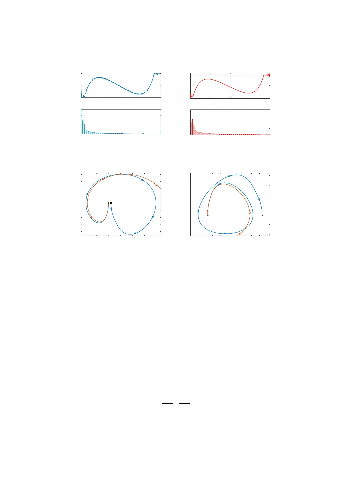
DISCRETE TIME OPTIMAL CONTROL WITH FREQUENCY CONST RAINTS FOR NON-SMOOTH SY STEM S SHR UTI K OTP ALLIW AR, PRAD YUMNA P AR UCHURI, DEB ASISH CHA T TERJEE, AND RA VI B AN A V AR December 20, 2024 Abstra ct . W e present a Po ntrya gin maximum pr inciple for discret e time opti mal control problems with (a) pointwise constraint s on the control actions and the state s, (b) smooth frequ ency c onstra ints on the control and the state traj ectories, and (c) nonsmoot h dynamical sys tems. Pointwi se cons traint s on the sta tes and the control actions represe nt desired and/or ph y sical limitati ons on the states and the control va lues; such const raints are impor tant and are widel y present in the opti mal control literatu re. Constr aints of the type (b), while less stand ard in the litera ture, eﬀectiv el y ser v e the pur pose of describing impor tant properties of ine rtial actuat ors and sys tems. The conj unctio n of constrai nts of the type (a) and (b) is a relati v el y ne w phenomenon in optimal cont rol but are important f or the synthesi s contro l tra jec tories with a high degree of ﬁdeli ty . T he maximum princ iple establi shed here pro vides ﬁrst order necessary conditi ons f or optimality that serve as a star ting point f or the synthesis of control traje ctories corresponding to a larg e class of constrai ned motion plannin g problems that hav e high accu racy in a computation all y tracta ble fashi on. Moreo v er , the abil ity to handle a reasonabl y larg e class of nonsmooth dynamical syst ems that arise in practice ensures broad appli cabili ty of our theory , and we include sev eral illus tratio ns of our results on standard problems. 1. Introduction Optimal contro l the o r y , arguably , s tar ted in the av atar of the Brachy s tochrone prob le m of J. Berno ulli in the late 17th centur y [ S W97 ], and o v er the inter v ening centur ies has ev ol v ed into a subject that oﬀe rs a pow erful set of tools for con trol syn thesis. Especially relev ant in the context of practical ap plications are synthesis techniques that seamlessly integ rate constraints on the states an d control actions while maintaining computatio nal tractability . The literature on such constrained p r oblems is ce rta in l y not as vas t as th e counter p a rt f or uncon strained prob lems, and o ur ar ticle co n tr ibutes to precisely this body of w ork. Under the ov erarching stipulation of compu tationally tractable control synth e sis te ch- niques, there are tw o speciﬁc con tr ib utions of our w ork. The ﬁrst con cer ns the simultaneou s inclusion o f the follo wing f our diﬀerent classes of constraints in con trol prob lems: ◦ con straints on th e con trol action s poin twise in time, ◦ con straints on th e states pointwise in time, ◦ frequen cy constraints on the contro l trajectories, an d ◦ frequen cy constraints on the state trajectories. Key wor ds and phra ses. frequ ency constraints, optimal control, Pontry agi n maximum principle, nonsmooth sys tems. The authors w ere supported partiall y by the grant 17ISR OC001 from the Indian Space Rese arc h Organiz ation . The y thank Soumitro Banerjee f or useful pointer s to the lite rature on control of pow er electronic circ uits, and Karmvir Singh Phog at f or helpful discussions and access to his softw are . 1 2 S. K OTP ALLIW AR, P . P ARUCHURI, D. CHATTERJEE, AND R. B ANA V AR Each of th ese four ty pes of constraints is extremely impor tant in practical applicatio ns. Actuators are go v ern ed by th e law s o f phy sics a n d canno t deliver sig n als with magnitudes that are bey ond their physical limitations; this natur a lly mea n s th at the set of ad missible control action s is constrained. Controlled dyn amical systems ar e typically per mitted to operate o nly within reasonable bo u ndar ies to av oid fatigue, p r emature ageing and disinte- gratio n of their compo nents; this natur a lly imp oses constraints on their states . Frequency constraints on the contro l trajectories are need ed for all iner tial actu ators, without which the syn thesized con trol sign als m ay con ta in fr equencies that cannot be faithfull y r e p ro- duced by the actuato rs du e to their physical limitations; in such cases, diﬀeren ces ar ise between the predicted and obser ved behaviours, leading to loss o f precision in the ir desired per f or mances. T o take care of this issue, frequen tly in practice, the synth esized contro ls are passed through a ﬁlter located before the actuator to en sure satisfaction o f the desired spectr um. This proced ure, how e v er , distor ts the or igin al signal that was design ed with the desired per f or mance objectives in mind, an d hen ce the sy stem per form ance d eter iorates. Frequency co nstraints on the state trajector ies are relev ant in iner tial contr o lled sys tems: they ar e espec iall y useful to prev ent undesirable vibration s of ﬂe xible str uctures in mechan- ical objects such as satellites, aeroplanes, robotic ar ms, or to induce d esirable d amping in ﬂe xible struc tu res, e tc . , and v ibration control has b e en an active area of con tr ol f or the past se v eral d ecades. On the one hand, the ﬁrst two ty p es of constraints hav e been studied e xtensiv el y in the co nte xt of optimal co ntrol, and are, to a fair extent, amena b le to computatio n ally c on- structive synthesis techniques. Indeed , con tr ol actio n constraints are common place in optimal co ntrol theo r y: bo th th e Pontr yagin maximu m pr inciple and d ynamic p rogr am- ming techniques [ IT09 , Lib 11 , Dub78 , DM6 5 , Ber12 ] p er mit the i nclusion of control action con straints po in twise in time. Wh ile dyn a mic pr ogra mming is not alwa y s compu- tationally tra c table (e. g., for hig h-dimen sional sys tems), there are n umer ical algo r ith ms that employ th e P ontr yagin maximu m pr inciple to synthesize constrained optimal control trajectories. Alg or ithmic techniques relying on v iability theo r y [ ABSP11 ], while compu ta- tionally demandin g (to the po int of being prohib itiv e f or high-dimen sional sy stems), per mit the inc lu sion of state constraints pointwise in time in addition to contro l co nstraints. On the other h and, the inclusion of f r equency constraints on th e control an d state trajector ies is relativ ely uncommo n in the literature. Despite the fact that the classical feedbac k techniques of continuo us-time H ∞ control [ DFT92 ] d o deal with frequency doma in beh aviour of the control tra jector ies and are capable o f in directly realizing restrictions on fr equency comp o- nents via penalization of cer tain ba n ds, neither shar p cut-oﬀs in the spectru m no r control and st ate constraints c a n be readily en f orced via this technique. Frequency constraints on the state trajectories, especially in th e context of nonlinea r systems, hav e be e n treated sparsely in th e literature; ty pical exist ing appro aches r el y o n fr equency doma in techniques that are ill-suited to h a ndle state and control constraints and are diﬃcult to app l y to non lin - ear sys tems. I n fact, apar t f r om the U S Patent [ SB95 ], we are u naw are o f e xtensive studies that impose frequency constraints on the states and contro l trajector ies. In par ticular, our o wn p r evious studies [ PC19 , K PP + 18 ] hav e only focussed on freque n cy constraints on th e control trajectories, an d the simultaneou s inclusion o f time and frequenc y constraints with precise bounds a n d cut-o ﬀs on frequen cy bands ar e not to be f ound in the e xis ting literature to th e best of our k no w ledge. Our cur r e nt results add ress these lac u nae: w e establish a v ersion of the P ontr yagin m a x imum pr incip le f or optimal control of discrete time n o nlinear control systems for wh ich the af orementio ned con straints are all enforced simultane o usly . These constraints are speciﬁcally illu strated in § 6.1 on a linear ap proximation of an inv erted pendu lu m on a car t aro und th e unstable equilibr ium p osition of the pend ulum. W e specif- ically impose state constraints so that the validity of the linear ization is maintained , and demonstrate that simple point-to- p oint man o euvres are dram atically altered by an ad -hoc poster io r i application of fr equency ﬁlters. DISCRETE TIME OPTIMAL CONTROL WITH FREQUENCY CONSTRAINTS 3 The second speciﬁc con tr ib ution of this ar ticle is the ability to encompass no nsmooth problem data. Nonsmooth dynamical systems ar ise naturally in a variety of application areas [ AB08 ], in cluding those wh e re the physical character istics of devices in v olv e nonlin ear ities such as the nor m ins tead of its square [ GP17 ], or wh en the d ynamical eq uations are deﬁned piece- wise o v er disjoint do mains of the state-space as a result o f intr insic p roper ties of d evices [ BKYY00 ]. The Pontr yagin max imum pr inc iple established in th is ar ticle, although not cater ing to th e mo st general situation insofar as no nsmoothn ess is co ncer ned, handles a large class o f nonsm o oth no nlinear ities that ar ise in pr actical applications. 1 T his speciﬁc aspect of our results is illustrated on two ex amples in § 6 : a standard non-smo o th dynamica l sys tem and the popular buck conv erter p ow er electron ic circuit. The optimal co ntrol synthesis pro cedure p resented in this article proceeds with models in discrete time. W e presum e that these discrete time models faithfully represent the dynamics of the sys tem, and do not concer n ourselv es here with the issues of discretization of continuo us-time sys tems. Our pr e ference for discrete time m odels is motivated by two factors, the ﬁrst of wh ich is the obser vation that the ﬁn a l implem entation of contr ollers are car r ied out digitally via samp le-and-h o ld mechanisms, and the ref ore, naturally inv ol v es a time discretization . Th e other factor is essentially that of convenience: the mathematical and numer ical com p le xity in v olv ed in inco rp orating the f our types of co nstraints that w e want in th e continuou s time is f or midable if not outr igh t impossible. This ar ticle un f olds as f ollo w s: W e provide in § 2 a precise mathem atical s tatement of our op timal problem that incor po rates pointwise constraints on the states and the control actions, and fr equency constraints on the control and the state trajectories, f or a large class of no n smooth dyn amical sys tems. § 3 co nsist of a set of prelimin ar ies n eeded for the pro of of m ain result. In § 4 w e establish a set of ﬁrst order nece ssary conditions for optimality in th e optimal contr ol prob lem deﬁned in § 2 ; th is is th e central contr ibu tion of this ar ticle. W e f ollo w up with som e technical remark s and immediate corollar ies. § 5 is de v oted for the detailed proof of main result, and in the ﬁnal § 6 w e p resent se v eral e xamples to illustrate the pro posed necessar y cond itio ns. Th e appen d ices § A and § B consist of sev e ral auxiliar y results tha t are employ ed in the proo f of our main result. 2. Problem Setup Consider a discr ete time co n trol sys tem whose d ynamics is g o v ern ed by th e diﬀerence equation (2.1) x t + 1 = f t ( x t , u t ) f or t = 0 , . . . , N − 1 , with th e follo wing data: ( 2.1 -a) x t ∈ R d is the vector of state at tim e t , ( 2.1 -b) u t ∈ R m is th e vector of contro l action at time t , ( 2.1 -c) R d × R m ∋ ( ξ , µ ) 7− → f t ( ξ, µ ) ∈ R d f or t = 0 , . . . , N − 1 , is a given famil y of locally Lipschitz contin u ous maps. In this article we der ive ﬁrst order necessary cond itions —a Pontr yagin Maximum Pr in- ciple—for discrete time o ptimal contro l pr oblems with nonsmo oth d ynamics and fre quency constraints on th e state and contro l trajectorie s in additio n to the standard constraints on the control m a gnitudes an d the states. The constraints on the frequencies of the states and con trol trajector ies r e f er to constraints o n th e discrete F our ier tran sf orm (DFT s) of th e individu al compon ents of the states an d co ntrols. Con straints on the f requency spectra of the con trol tra jector ies appeared in the [ PC19 ]; h ere we mo v e o ne step fur ther by p er mitting constraints on the spectra of the state trajector ies, to be present as a given stipulation. 1 See also the discussion immediatel y prece ding ( 2.2 ) concerning possible genera liza tions. 4 S. K OTP ALLIW AR, P . P ARUCHURI, D. CHATTERJEE, AND R. B ANA V AR In addition to hand ling freque ncy con straints, o u r r esult also encom passes piecewise smooth dy namical system such as the ones men tioned in § 1 , and according l y , we per mit our dy namics to be nonsmooth . A more general fr amew o rk where both th e cost-per -stag e and the dy namics ar e nonsmo oth, is possible, and such a general framew ork is typically employ ed to compare the nece ssar y condition s f or a discrete time o ptimal con trol pro blem and a discrete time approximation of a con tinuous time problem; see, e.g., [ Mor06b ]. W e do not aim f or maximal generality in our w ork pr im ar il y to en sure a clean calcu lus; in fact, some of ou r assumptions are aime d a t simplify ing th e necessar y cond itio ns that ar ise in more general situatio ns. Here is th e pr e c ise mathem atical statement of ou r prob lem: (2.2) minimize ( u t ) N − 1 t = 0 N − 1 Õ t = 0 c t ( x t , u t ) + c N ( x N ) subject to                    dynamics ( 2.1 ) , x t ∈ S t f or t = 0 , . . . , N , u t ∈ U t f or t = 0 , . . . , N − 1 , F ( x 0 , . . . , x N ) = 0 , G ( u 0 , . . . , u T − 1 ) = 0 , where ( 2.2 -a) the mappin g R d × R m ∋ ( ξ , µ ) 7− → c t ( ξ, µ ) ∈ R f or each t = 0 , . . . , N − 1, is continuo usly diﬀe r entiable and deﬁnes a sequence of cost pe r stage fu nctions, and R d ∋ ξ 7− → c N ( ξ ) ∈ R is a continu ously diﬀe r entiable ﬁnal stage cost, ( 2.2 -b) ( S t ) N t = 0 is a sequence of closed subsets of R d descr ibing a tube (o v er tim e) of admissible states, ( 2.2 -c) ( U t ) N − 1 t = 0 is a sequence of clo sed subsets of R m depicting the sets of adm issible control actions at each time t , ( 2.2 -d) given ν x ∈ N , some v ector Υ x ∈ R ν x , and smoo th functions e F t : R d → R ν x f or t = 0 , . . . , N , we deﬁn e the map R d ( N + 1 ) ∋ ( ξ 0 , . . . , ξ N ) 7− → F ( ξ 0 , . . . , ξ N ) ≔ Υ x + Í N t = 0 e F t ( ξ t ) ∈ R ν x (this map F w ill b e emplo y ed to quantify constraints on the f requency spectra of the state trajector ies), ( 2.2 -e) given ν u ∈ N , some vector Υ u ∈ R ν u , an d smoo th f unctions e G t : R m → R ν u f or t = 0 , . . . , N − 1, w e deﬁne the map R m N ∋ ( µ 0 , . . . , µ N − 1 ) 7− → G ( µ 0 , . . . , µ N − 1 ) ≔ Υ u + Í N − 1 t = 0 e G t ( µ t ) ∈ R ν u (this map G will be em plo y ed to quan tify constraints on the fr e quency spectra of the control trajectories). Remark 2 .1 . For the control tra jector y ( u t ) N − 1 t = 0 , let u ( k ) ≔ ( u ( k ) t ) N − 1 t = 0 denote the tra jector y of the k th compon ent o f the control for each k = 1 , . . . , m . For each com ponent trajectory u ( k ) , we ob tain the v ector of DFT co eﬃcients d u ( k ) ≔ F u ( k ) ∈ C N where F ∈ C N × N denotes th e DFT matrix cor respond ing to signal length N (see [ SS03 , Chap ter 7]). Let b u ≔  c u ( 1 ) ⊤ c u ( 2 ) ⊤ . . . d u ( m ) ⊤  ⊤ ∈ C m N denote the vector of stac k ed frequency co e ﬃecients of all compo nents u ( k ) , k = 1 , . . . , m . T hat is, C m N ∋ b u ≔ ©    « c u ( 1 ) . . . d u ( m ) ª ® ® ® ¬ = ©   « F u ( 1 ) . . . F u ( m ) ª ® ® ¬ By fre que n cy constraints on the contro l tra jector y , we refer to con straints on the DFT coeﬃcients of the traj ector ies of th e co mponen ts of control. W e specialize our results in this ar ticle to co nstraints that elimin ate ce r tain frequen cy com ponents of the contr ol tra jector ies, DISCRETE TIME OPTIMAL CONTROL WITH FREQUENCY CONSTRAINTS 5 i.e., restr ict cer tain entr ies of b u to zero. By carefully choosing the ro w s cor respon ding to the desired f r equency comp onents to be restricted, separating the real and im aginar y par ts, and using a suitable rear r angement, one obtains co nstraints of the form mentioned in (2.2-e) , with ν u denoting the nu mber of entrie s of b u being restricted, counting real and im a ginar y par ts separately , and the maps e G t being the linear transform ations co ntaining the row s of DFT matr ix in a speciﬁc arran gement. In our presentation, we generalize this class of constraint maps, e G t , to be ju st smooth . For mo re d etailed explanation see [ PC17 ]. The frequen cy co nstraints on the state tra jector ies descr ib ed in (2.2-d) are obtained in a similar mann er . If o ne were to consider th e DFT coeﬃcients, one needs to use the DFT matr ix cor resp onding to a signal of length N + 1. In the sequel we refer to the sequence ( u t ) N − 1 t = 0 as a con tr ol tra jectory , with u t being the control action at time t . 3. Preliminaries In th is section w e re view som e elementar y facts from an aly sis in a nonsmoo th setting; we ref er the read er to [ CLS W98 , HUL93 , Gü l10 ] for fur th er inf or mation on th is to pic. F or us h· , ·i r ef ers to the usu al inne r prod uct in R n and k · k to th e nor m in duced by h· , ·i . F or ǫ > 0 and x ∈ R n , B ǫ ( x ) refers to the op e n ball { y ∈ R n | k y − x k < ǫ } of radius ǫ centered at x . A function g : R n − → R is said to be Lipschitz con tinuous nea r x ∈ R n if there e xis ts r , L > 0 such that | g ( y ) − g ( z ) | 6 L k y − z k f or all y, z ∈ B r ( x ) . A set S ⊂ R n is conv ex if f or all x , y ∈ S and for all α ∈ [ 0 , 1 ] , we hav e ( 1 − α ) x + α y ∈ S . A nonem pty set K ⊂ R n is a cone if f or ev er y y ∈ K and for ev ery α > 0 , w e hav e α y ∈ K . A set K ( x 0 ) ⊂ R n is a cone with vertex x 0 ∈ R n if f or all α > 0 and f or all y ∈ K ( x 0 ) , α ( y − x 0 ) ∈ K ( x 0 ) . For a conv e x cone K ( x 0 ) ⊂ R n with verte x x 0 , its dual cone K ( x 0 ) + is deﬁned v ia po lar ity by K ( x 0 ) + ≔  y ∈ R n   h y, x − x 0 i 6 0 f or all x ∈ K ( x 0 )  . Deﬁnition 3.1. [ Cla13 , Section 1. 4 on p. 20 ] L e t g : R d × R m − → R n be a co ntinuous map and g 1 , . . . , g n are its comp o nents. For y ∈ R m and a v ector v ∈ R d , we d enote by D v g ( · , y )( x ) the directional d erivativ e of g ( · , y ) along v at x , wh enev er the f ollo wing limit e xists: D v g ( · , y )( x ) ≔ lim θ ↓ 0 g ( x + θ v, y ) − g ( x , y ) θ (3.1) =  lim θ ↓ 0 g 1 ( x + θ v, y ) − g 1 ( x , y ) θ , . . . , lim θ ↓ 0 g n ( x + θ v, y ) − g n ( x , y ) θ  ⊤ W e note th at the d ir ectional der ivativ e abov e is deﬁned as a rig ht-hand (one- sided) lim it. If g is continu ously diﬀerentiab le, then D v g ( · , y )( x ) = ∂ ∂ x g ( x , y ) . v . How e v er , there a r e Lipschitz function s for which the left-hand and r ight-han d limit exist f or all the directio ns at a po int x (which h appens if the function is co ntinuous at x ), but they a r e no t equal i.e., lim θ ↓ 0 g ( x + θ v )− g ( x ) θ , lim θ ↑ 0 g ( x + θ v )− g ( x ) θ . For example, for the absolute value f u nction R ∋ x 7− → f ( x ) = | x | ∈ R at x = 0, D v f ( 0 ) = | v | = ( v f or v > 0 , − v f or v < 0 , and lim θ ↑ 0 f ( 0 + θ v )− f ( 0 ) θ = − | v | . Of co urse, | · | is not Gateaux d iﬀerentiable at x = 0. 2 2 R ecal l that if the right-hand limit of g : R d × R m − → R n at x is equal to the left-hand limit at x then, the functio n g is Gateaux diﬀer ent iable at x . In this case, D v g ( · , y )( x ) = ∂ ∂ ξ g ( · , y )( x ) · v . 6 S. K OTP ALLIW AR, P . P ARUCHURI, D. CHATTERJEE, AND R. B ANA V AR Deﬁnition 3.2. If h : R n − → R is a Lipschitz continuo us fun ction, then the generalized directional derivative h ◦ ( x ; v ) of h a t x alo ng the directio n v is d eﬁned by h ◦ ( x ; v ) ≔ lim sup y → x t ↓ 0 h ( y + t v ) − h ( y ) t . In g eneral, the generalized dir ectional d er ivativ e takes values in R ∪ { + ∞ } . Th e generalized gradient ∂ h ( x ) o f h at x is a n onempty co mpact subset of ( R n ) ⋆ deﬁned by ∂ h ( x ) ≔  ξ ∈ ( R n ) ⋆   h ξ, v i 6 h ◦ ( x ; v ) f or all v ∈ R n  . Deﬁnition 3 . 3. A Lipschitz continuous fun c tion g : R d − → R is said to be r egular at x ∈ R d if the dire c tional der ivativ e o f g at x alon g any v ∈ R d e xists and is equal to its generalized directional d er ivativ e at x alo n g th at v , i.e., D v g ( x ) = g ◦ ( x ; v ) < + ∞ . W e look at tw o e xamples: ◦ Let R ∋ x 7− → f ( x ) ≔ max { 0 , x } ∈ R . It is clear that f is Lip schitz continuo us and is diﬀeren tiable ev erywh ere ex cep t at x = 0 . The directional der ivativ e, the g eneralized directional der ivativ e and th e generalized g radient o f f at 0 an d 1 are D v f ( 0 ) = f ( v ) , f ◦ ( 0; v ) = f ( v ) , ∂ f ( 0 ) = [ 0 , 1 ] , D v f ( 1 ) = v, f ◦ ( 1; v ) = v and ∂ f ( 1 ) = { 1 } . ◦ Let R d ∋ x 7− → f ( x ) ≔ k x k ∈ R . Clearl y , f is a L ipschitz continuou s f unction diﬀerentiab le ev erywh ere ex ce pt at 0. T he generalized direction a l d er ivativ e and the generalized grad ie n t of f at 0 are D v f ( 0 ) = k v k , f ◦ ( 0; v ) = k v k and ∂ f ( 0 ) = cl ( B 1 ( 0 )) . Note that the functio n s in th e abov e tw o examples are regular at 0 . Let S ⊂ R n be a nonemp ty and closed set. Th e distance d S ( x ) o f a point x ∈ R n from S is de ﬁn ed by R n ∋ x 7− → d S ( x ) ≔ in f s ∈ S k x − s k ∈ [ 0 , + ∞[ . Deﬁnition 3.4. The Clarke tangent and normal co nes to S at a point x ∈ S , deno ted by T C S ( x ) and N C S ( x ) respectivel y , are deﬁned as T C S ( x ) ≔  v ∈ R n   d ◦ S ( x ; v ) 6 0  , N C S ( x ) ≔  ξ ∈ ( R n ) ⋆   h ξ, v i 6 0 for all v ∈ T C S ( x )  . The Clark e tangent cone T C S ( x ) at x is a closed co nv ex set and th e no r mal cone N C S ( x ) at x is th e po lar o f the tangent cone T C S ( x ) . Intuitiv ely , the tangent cone at x to S is the set of directions along which it is possible to ‘enter’ S from x , and th e nor mal co ne provides the set o f direction s alo ng which on e can most e ﬃ ciently ‘exit ’ S from x . The Clarke tangent cone an d nor mal con e to the sets S 1 = { x ∈ R 2 | x 2 > | x 1 | } and S 2 = { x ∈ R 2 | x 2 6 2 | x 1 | } at or igin o = ( 0 , 0 ) are shown in Figure 1 . 4. Main resul t Assump tion 4.1. W e stipulate that the maps f t ’ s in (2.1-c) are r egular at every ( ξ, µ ) ∈ R d × m . DISCRETE TIME OPTIMAL CONTROL WITH FREQUENCY CONSTRAINTS 7 x 1 x 2 x 2 = | x 1 | o S 1 T C S 1 ( o ) N C S 1 ( o ) x 1 x 2 x 2 = 2 | x 1 | T C S 2 ( o ) S 2 N C S 2 ( o ) o Figure 1 . T angent cone to th e sets S 1 , S 2 at o = ( 0 , 0 ) Our main resu lt is th e follo wing theorem: 3 Theorem 4 .2. Consider the problem ( 2 . 2 ) alo n g with its associated data, and suppose t hat Assumption 4.1 holds. Let ( u ∗ t ) N − 1 t = 0 be a control tra jectory that solv es the o ptimal optimal control problem ( 2.2 ) , and let x ∗ ≔ ( x ∗ t ) N t = 0 be the corr esponding state traj ectory. Deﬁne the Hamiltonian (4.1) R × ( R ν x ) ⋆ × ( R ν u ) ⋆ × ( R d ) ⋆ × { 0 , . . . , N − 1 } × R d × R m ∋  α , ϑ x , ϑ u , ζ , s , ξ, µ  7− → H α , ϑ x , ϑ u ( ζ , s , ξ , µ ) ≔ h ζ , f s ( ξ, µ ) i − α c s ( ξ, µ ) − D ϑ x , e F s ( ξ ) E − D ϑ u , e G s ( µ ) E ∈ R . Then ther e exist • an adjoint tr aject ory ( η f t ) N − 1 t = 0 ⊂ ( R d ) ⋆ , • a sequence ( η x t ) N t = 0 ⊂ ( R d ) ⋆ , an d • a triplet  η c , c η x , c η u  ∈ R × ( R ν x ) ⋆ × ( R ν u ) ⋆ , satisfying (C-i) the non -negativity conditio n: η c ∈ { 0 , 1 } ; (C-ii) the non-triviality con dition: the adjoint tr aject or y ( η f t ) N − 1 t = 0 and the triplet  η c , c η x , c η u  do not simultaneou sly vanish; (C-iii) the state and a djoint dyn amics: x ∗ t + 1 = ∂ ∂ ζ H η c , c η x , c η u ( η f t , t , x ∗ t , u ∗ t ) for t = 0 , . . . , N − 1 , D η f t − 1 , y E > D y H η c , c η x , c η u ( η f t , t , · , u ∗ t )( x ∗ t ) −  η x t , y  for all y ∈ R d and some η x t ∈ N C S t ( x ∗ t ) , for t = 1 , . . . , N − 1; 3 In the seq uel there will arise the need to tak e par tial derivati v es of multiv ariable functions relativ e to speciﬁc v ariables, and w e tak e care to precisel y indicate the variabl es with respect to which w e tak e these partial der iv ativ es b y introducing dummy v ariable s in the deﬁniti ons. T he adjoint variabl es (a.k.a. ‘multipliers ’) cor respondin g to the cost, the dynamics, the sta te-con strai nts, and the frequenc y constr aints of the state and the contr ol trajec tories appear here, and we distingui sh betw een them by introduci ng the diﬀerent super -scripts of the single Greek lett er η . V arious objects in frequency space are distinguished b y a ‘hat ’ . While this mechanism leads to a multitud e of sub-/super -scripts, we belie ve that it ensures much-ne eded tra nsparency and tractabi lity . 8 S. K OTP ALLIW AR, P . P ARUCHURI, D. CHATTERJEE, AND R. B ANA V AR (C-iv) t he transver sality conditio ns: D y H η c , c η x , c η u ( η f 0 , 0 , · , u ∗ 0 )( x ∗ 0 ) −  η x 0 , y  6 0 for all y ∈ R d and some η x 0 ∈ N C S 0 ( x ∗ 0 ) , and η f N − 1 = − η c ∂ ∂ ξ c N ( x ∗ N ) −  ∂ ∂ ξ e F N ( x ∗ )  ⊤ c η x − η x N for some η x N ∈ N C S N ( x ∗ N ) ; (C-v) the Ha miltonian maximization cond ition: D p H η c , c η x , c η u ( η f t , t , x ∗ t , ·) ( u ∗ t ) 6 0 for a ll p ∈ T C U t ( u ∗ t ) and for t = 0 . . . , N − 1; (C-vi) fr eq uency co nstr aints on the state tra jectory ( x ∗ t ) N t = 0 : F ( x ∗ 0 , . . . , x ∗ N ) = 0; (C-vii) freq uency co n str aints on the co ntr ol a ction tra jectory ( u ∗ t ) N − 1 t = 0 : G ( u ∗ 0 , . . . , u ∗ N − 1 ) = 0 . A detailed proo f of Theore m 4.2 is postpone d to the next section. In the re m ainder of the cur ren t section we shall br ieﬂy d iscuss th e conditio n s (C-i) – (C-vii) in the forthcom ing remarks an d examine se v eral spec ia l cases of the main pro blem ( 2 . 2 ). Remark 4.3 . The scalar η c , called the a bnor mal multip lier , tak es the value 0 or 1. If η c = 0, then the extr emal lif t  η c , ( η f t ) N t = 0 , c η x , c η u , ( x ∗ t ) N t = 0 , ( u ∗ t ) N − 1 t = 0  cor respon d ing to an o ptimal pair  ( x ∗ t ) N t = 0 , ( u ∗ t ) N − 1 t = 0  is called an ab norma l ex tremal . I f η c = 1, then the cor respond ing the e xtremal lift is called no rmal . Remark 4 .4 . The en tr ies of th e sequen ce ( η f t ) N − 1 t = 0 are called adjoint v ectors or co -states; their ev olution is go v er ned by the adjo int dynamics (C-iii) , and the transversality conditions (C-iv) p r o vide its bo undar y conditions. Due to the no n smooth natu r e of the state dynam ics, the ad joint recursion is an inclusio n η f t − 1 ∈  η ∈ R d   h η , y i > D y H η c , c η x , c η u ( η f t , t , · , u ∗ t )( x ∗ t ) −  η x t , y  f or all y ∈ R d  as opposed to an equation. In Corollar y 4.9 we sh a ll o bser v e that if the dyn amics are continuo usly diﬀerentiab le, then this in clusion tur n s into an equation , which is the standard adjoint equatio n in the classical Pontryagin maximum pr in ciple. Remark 4 .5 . In the transversality con d ition (C-iv) the te r m s N C S 0 ( x ∗ 0 ) and N C S N ( x ∗ N ) are Clarke nor mal con es. Ho w e v er , there is a mo re general notion of a nor mal con e due to Morduk ho vich called the ba sic o r limitin g normal con e [ Mor06a , Chapter 1] , and the approximate discrete-time PMP in [ Mor06b ] p resents necessar y co nditions for optimality in ter ms of this limiting no r m al con e. Ou r appro ach of th e proof u ses th e conv e xity of the Clarke n or mal cone in a n essential wa y , while it is known that th e lim iting nor mal cone may fail to be conv e x; co nsequently , the result and its proo f pr o vided her e do e s not car r y o v er in an elegant fashion while inv ol ving the limiting n o r mal cone. Remark 4.6 . The sequen ce of multip lier s ( η x t ) N t = 0 cor respon d to th e pointwise state con - straints. The deﬁnition ( 4.1 ) o f th e Hamilto nian features tw o n ew ter ms, D ϑ x , e F s ξ E and D ϑ u , e G s µ E , compared to the standard deﬁnition (e.g., [ Bol75 ]). These ter ms acco unt for the frequency constraints on the state trajectory and the c o ntrol trajectory , respectivel y . One similar term also app eared in the Hamiltonian in [ PC19 ], where frequency constraints on the control tr aj ector ies were co nsidered. The v ectors c η x , c η u are th e multip liers cor resp onding to th e fr e quency constraints o n the states and the con trols, respectivel y . DISCRETE TIME OPTIMAL CONTROL WITH FREQUENCY CONSTRAINTS 9 Remark 4. 7 . The condition ( C-v) s tates that at ev ery t th ere e xis t a n e ighborh ood of u ∗ t (say B ǫ ( u ∗ t ) ) such that H η c , c η x , c η u ( η f t , t , x ∗ t , u ∗ t + p ) 6 H η c , c η x , c η u ( η f t , t , x ∗ t , u ∗ t ) for all p ∈ B ǫ ( u ∗ t ) ∩ T C U t ( u ∗ t ) . The Clark e tangent cone T C U t ( u ∗ t ) provides a c onv e x conic approximation of th e set U t at the point u ∗ t . (Here the ter m approximation of a set U t at a po in t u ∗ t stands for a set of d irections along wh ich it is possible to en ter the set U t from th e poin t u ∗ t .) Th e n the condition (C-v) implies th at the value Ham ilto nian at u ∗ t is g reater than the value Hamiltonian at the points in the co nv ex conic approximation of the set U t at the point u ∗ t and that are close to u ∗ t . Consequently , (C-v) do es not imply Hamiltonian max imization which is a well-kno wn pheno m enon in the discrete time optim al c ontrol literature [ MS04 , Pše71 ]. Although not entirely ap propr iate, we call this condition “the Hamilton ian maximiza tio n ” to maintain a similar ity with the continu ous time PMP . Besides, und e r suitab le fur ther assumptions on the admissible contr ol action set, (C-v) implies max im ization of the Hamilton ian. I n deed, if the admissible set U t is c o nv e x and co mpact, then U t ⊂ T C U t ( u ∗ t ) , an d the co ndition (C-v) simpliﬁes to at ev ery t there exis t a neig hborh o od o f u ∗ t , i.e., B ǫ ( u ∗ t ) , su ch that H η c , c η x , c η u ( η f t , t , x ∗ t , u ∗ t + p ) 6 H η c , c η x , c η u ( η f t , t , x ∗ t , u ∗ t ) for all p ∈ B ǫ ( u ∗ t ) ∩ U t . In othe r w ords, u ∗ t is a local maxim izer o f the Hamiltonian at time t . Theref ore, if we assume tha t at each t the Ham iltonian 4.1 is con cav e with respect to the co n trol variab le then the condition (C-v) implies the lo cal maximizatio n of th e Hamilto nian at each instant along th e op timal trajector ies. Corollary 4.8 . Suppose that  η c , ( η f t ) N t = 0 , c η x , c η u , ( x ∗ t ) N t = 0 , ( u ∗ t ) N − 1 t = 0  is an extremal of ( 2.2 ) and let H η c , c η x , c η u be the Hamiltonian deﬁned in ( 4.1 ) . (i) If the dyna mics f i in (2.1-c) for ev ery i ∈ { 1 , . . . , N − 1 } are smooth with respect to the state variable ξ at x ∗ i , then the ad joint d ynamics in (C-iii) of Th eorem 4.2 at t = i str engthens to the recur sion η f i − 1 = ∂ ∂ ξ H η c , c η x , c η u ( η f i , i , x ∗ i , u ∗ i ) − η x i for some η x i ∈ N C S i ( x ∗ i ) . (ii) If the dynamics f 0 in (2.1-c) is smooth with respect to the state variable ξ at x ∗ 0 , then the transv ersality condition (C-iv ) of Theorem 4.2 str engthens to: ∂ ∂ ξ H η c , c η x , c η u ( η f 0 , 0 , x ∗ 0 , u ∗ 0 ) = η x 0 for some η x 0 ∈ N C S 0 ( x ∗ 0 ) , η f N − 1 = − η c ∂ ∂ ξ c N ( x ∗ N ) −  ∂ ∂ ξ e F N ( x ∗ )  ⊤ c η x − η x N for some η x N ∈ N C S N ( x ∗ N ) . (iii) If the dynamics f j in (2.1-c) f or e very j ∈ { 0 , . . . , N − 1 } are smooth with r espect to the control variable µ at u ∗ j , then the Hamiltonian maximization (C-v) cond ition in Theorem 4.2 at t = j simp liﬁes to:  ∂ ∂ µ H η c , c η x , c η u ( η f j , j , x ∗ j , u ∗ j ) , p  6 0 for all p ∈ T C U j ( u ∗ j ) . Proof. (i) For i ∈ { 1 , . . . , N − 1 } if the d ynamics (2.1-c) is smooth with respect to ξ at x ∗ i then H a miltonian H η c , c η x , c η u in ( 4.1 ) is smooth with respect to ξ at x ∗ i . Since the Hamiltonian is smooth at x ∗ i , the dire c tional der ivativ e of H η c , c η x , c η u ( η f i , i , · , u i ) at x ∗ i in any dire c tio n y ∈ R d is th e inn er prod uct of th e g radient of H η c , c η x , c η u ( η f i , i , · , u i ) at 10 S. K OTP ALLIW AR, P . P ARUCHURI, D. CHATTERJEE, AND R. B ANA V AR x ∗ i and y . In other words, ref err in g to the deﬁnition o f the Hamiltonian H η c , c η x , c η u in ( 4.1 ) an d the d ir ectional der ivativ e in ( 3. 1 ), D y H η c , c η x , c η u ( η f i , i , · , u ∗ i )( x ∗ i ) =  ∂ ∂ ξ H η c , c η x , c η u ( η f i , i , x ∗ i , u ∗ i ) , y  . The condition (C-iii) of T h eorem 4 .2 on adjo int dy namics gives us  η f i − 1 − ∂ ∂ ξ H η c , c η x , c η u ( η f i , i , x ∗ i , u ∗ i ) + η x i , y  > 0 for all y ∈ R d . Since the inner product is linear in y and the pre c e ding inequality is tru e for all y ∈ R d , we may replace y with − y in the ab o v e inequality , lead in g to η f i − 1 − ∂ ∂ ξ H η c , c η x , c η u ( η f i , i , x ∗ i , u ∗ i ) + η x i = 0 as desired. (ii) For t = 0 if th e dy namics (2.1-c) is smooth with respect to s tate var iable ξ at x ∗ 0 then the Hamiltonian H η c , c η x , c η u in ( 4.1 ) is con tinuously diﬀer entiable with respect to ξ at x ∗ 0 . Therefore, th e directional der ivativ e of Hamilton ian H η c , c η x , c η u ( η f 0 , 0 , · , u 0 ) at x ∗ 0 in any direction y ∈ R d is D y H η c , c η x , c η u ( η f 0 , 0 , · , u ∗ 0 )( x ∗ 0 ) =  ∂ ∂ ξ H η c , c η x , c η u ( η f 0 , 0 , x ∗ 0 , u ∗ 0 ) , y  . Then the tran sv ersality condition (C-iv) of Theor em 4 .2 and the linear ity of the abov e inner p roduct with resp ect to y leads to ∂ ∂ ξ H η c , c η x , c η u ( η f 0 , 0 , x ∗ 0 , u ∗ 0 ) = η x 0 . (iii) For j ∈ { 0 , . . . , N − 1 } if the dynamics f j in (2.1-c) is smooth with r espect to the control v ar iable µ a t u ∗ j , then we can wr ite the directional der ivativ e o f the Hamiltonian H η c , c η x , c η u ( η f j , j , x ∗ j , ·) with respect to control variab le µ at u ∗ j along th e direction p as the in ner produ ct D p H η c , c η x , c η u ( η f j , j , x ∗ j , ·)( u ∗ j ) =  ∂ ∂ µ H η c , c η x , c η u ( η f j , j , x ∗ j , u ∗ j ) , p  . Then for t = j the Hamiltonian maximization con dition (C-v) o f Th eorem 4 .2 special- izes to  ∂ ∂ µ H η c , c η x , c η u ( η f j , j , x ∗ j , u ∗ j ) , p  6 0 .  Remark 4 . 9 . Suppose that in ( 2.2 ) w e rep lace th e L ipschitz con tinuous dy namics hypothesis (2.1-c) o f ( 2.1 ) with each R d × R m ∋ ( ξ, µ ) 7− → f t ( ξ, µ ) ∈ R d f or t = 0 , . . . , N − 1 , being contin uously d iﬀerentiable, then the H a m iltonian as deﬁned in ( 4.1 ) is continuou sl y diﬀerentiab le in ξ and µ . In this setting , th e conditions (C-iii) , (C-iv) an d (C-v) of Theo rem 4.2 can be s trengthe n ed to (iii ∗ ) , (iv ∗ ) and (v ∗ ) respectivel y , giv en below : (iii ∗ ) state and adjo in t dynam ics: x ∗ t + 1 = ∂ ∂ ζ H η c , c η x , c η u ( η f t , t , x ∗ t , u ∗ t ) for t = 0 , . . . , N − 1 , η f t − 1 = ∂ ∂ ξ H η c , c η x , c η u ( η f t , t , x ∗ t , u ∗ t ) − η x t f or som e η x t ∈ N C S t ( x ∗ t ) an d for t = 1 . . . , N − 1; DISCRETE TIME OPTIMAL CONTROL WITH FREQUENCY CONSTRAINTS 11 (iv ∗ ) transv ersality condition s: ∂ ∂ ξ H η c , c η x , c η u ( η f 0 , 0 , x ∗ 0 , u ∗ 0 ) = η x 0 f or all y ∈ R d and f or some η x 0 ∈ N C S 0 ( x ∗ 0 ) , η f N − 1 = − η c ∂ ∂ ξ c N ( x ∗ N ) −  ∂ ∂ ξ e F N ( x ∗ )  ⊤ c η x − η x N f or some η x N ∈ N C S N ( x ∗ N ) ; (v ∗ ) Hamilton ian maximiz a tion condition :  ∂ ∂ µ H η c , c η x , c η u ( η f t , t , x ∗ t , u ∗ t ) , p  6 0 f or all p ∈ T C U t ( u ∗ t ) an d for t = 0 . . . , N − 1 . W e h av e a second (imme d iate) special case, whose p roof follo w s at onc e fro m the precedin g d iscussion. Corollary 4.10 . If the controlled sys tem in ( 2.2 ) is line ar , that is, ( 2.1 ) is replaced by x t + 1 = A t x t + B t u t where A t ∈ R d × d and B t ∈ R d × m for t = 0 , . . . , N − 1 , then for the Hamiltonian d eﬁned in ( 4.1 ) , the assertions of Theo r em 4 .2 h o ld wit h the ad jo int dynamics in (C-iii) g iv en by (4.2) η f t − 1 = A ⊤ t η f t − η c ∂ ∂ ξ t c t ( x ∗ t , u ∗ t ) − e F t ( x ∗ t ) ⊤ c η x − η x t for t = 0 , . . . , N − 1 . Moreo v er , if each U t is no n-empty, co nvex, and comp act, then the cond ition (C-v) in Theorem 4.2 becomes the standa r d Hamiltonian maximizatio n cond ition H η c , c η x , c η u ( η f t , t , x ∗ t , u ∗ t ) = max µ ∈ U t H η c , c η x , c η u ( η f t , t , x ∗ t , µ ) for t = 0 , . . . , N − 1 . The f ollo wing resu lt addresses the optimal contr ol p roblem ( 2.2 ) under a diﬀeren t set of hypotheses than Assum p tion 4.1 . Here we assume that • the dyn amics are smooth a nd • the cost fu nctions are regu lar but m ay be n onsmooth while re taining the r est o f the problem d a ta. W e obser ve that the necessar y c o nditions for this modiﬁed prob lem are similar to the necessar y conditio n s in Th eorem 4. 2 ex cept the transversality conditions; these necessary condition cater to, e.g., ℓ 1 -minimization problems that m a y be em plo y ed to enforce sparsity . The pr ecise statement is a s follo w s: Theorem 4. 11. Con sider the problem ( 2.2 ) with the following modiﬁc a tions: (a) the functions f t in ( 2.1 ) a r e con tinuously diﬀerentiable everywhere, and (b) the fun ctions c t in ( 2 .2-a) are regular at every ( ξ, µ ) ∈ R d × m . 4 Let ( u ∗ t ) N − 1 t = 0 be a control tr a jectory that solves t he optimal optimal control pr oblem ( 2 .2 ) with the modiﬁcation s (a) and (b ) , and let x ∗ ≔ ( x ∗ t ) N t = 0 be the corresponding s tate tra jectory. Then, for the Hamiltonian deﬁned in ( 4.1 ) , there exist • an adjoint tr aject ory ( η f t ) N − 1 t = 0 ⊂ ( R d ) ⋆ , • a sequence ( η x t ) N t = 0 ⊂ ( R d ) ⋆ , an d • a triplet  η c , c η x , c η u  ∈ R × ( R ν x ) ⋆ × ( R ν u ) ⋆ , satisfying (i) the non -negativity conditio n η c ∈ { 0 , 1 } ; (ii) the n on-triviality condition the ad joint tra jectory ( η f t ) N − 1 t = 0 and the triplet  η c , c η x , c η u  do not simultaneou sly vanish; (iii) the state and a djoint dyn amics (C-iii) ; 4 W e emphasize that the assumption of cont inuous diﬀerent iabil ity of the cost functio ns is being remov e d; conseq uentl y , c t ma y fail to be diﬀerentia ble at som e ( ξ, µ ) ∈ R d × m . 12 S. K OTP ALLIW AR, P . P ARUCHURI, D. CHATTERJEE, AND R. B ANA V AR (iv) t he transver sality cond itio ns D y H η c , c η x , c η u ( η f 0 , 0 , · , u ∗ 0 )( x ∗ 0 ) −  η x 0 , y  6 0 for all y ∈ R d and some η x 0 ∈ N C S 0 ( x ∗ 0 ) , and D η f N − 1 , y E + η c D y c N ( x ∗ N ) +   ∂ ∂ ξ e F N ( x ∗ )  ⊤ c η x + η x N , y  > 0 for all y ∈ R d and some η x N ∈ N C S N ( x ∗ N ) ; (v) the Ha miltonian maximization cond ition (C-v) ; (vi) fr eq uency co nstr aints on the state tra jectory ( x ∗ t ) N t = 0 (C-vi) ; (vii) freq uency co nstr aints on the co ntrol action tra jectory ( u ∗ t ) N − 1 t = 0 (C-vii) . Proof. A pro of of the abov e theorem follo w s the steps o f the pr oof of the Th eorem 4.2 giv en in the next section; we o mit the details in the inter e st of brevity . The proof will f ollo w the steps similar to the pro o f of Theo rem 4. 2 p resent in th e ne xt section. T o summar ize, we start with Step I in § 5.1 , an d follo w S tep II in § 5.2 un til th e Claim. In the Claim itself, the nonsmoo th cost and sm ooth dynamics are changed from ( 5.12 ) into the f ollo wing cond ition: 0 ∈ η c ∂ C ( z ∗ ) + ∂ ∂ z  λ f , f d (· )  ( z ∗ ) +  ∂ ∂ z b F ( z ∗ )  ⊤ c η x +  ∂ ∂ z b G ( z ∗ )  ⊤ c η u + N C Ω ( z ∗ ) . F or th e abov e new condition, we deﬁne th e func tion h ( z ) ≔ Í N − 1 t = 0 h t ( z ) = Í N − 1 t = 0 η c c t ( x t , u t ) and continu e S tep II, f ollo wed by Step III in § 5.3 to ar r ive at the end result.  5. Proof of Theorem 4.2 In this section we provide a detailed proo f of the main result Theorem 4.2 . Flo w char t 2 giv es an idea of a pr oof, and we elabor a te the main steps below : Sk etc h of the proof: W e p r oceed as per the three steps below : S tep (I) Our o ptimal co ntrol prob lem is lifted to an equivalent optimization pro blem in a suitable h igh-dim e nsional product space. S tep (II) Firs t ord er n ecessar y co nditions f or the o ptimization pro blem in S tep (I) are o b- tained using Clark e’ s necessar y co ndition f or no n-smooth o ptimization problems. S tep (III ) The necessar y conditions obtained in Step (II ) are projected to appropr iate f actors to ar r ive at n ecessar y cond itio n of th e or iginal contro l prob le m . 5.1. Step (I) . Equiv alent o ptimizatio n problem: The o bjectiv e of this step is to tr ansf or m the o r ig inal optimal control problem ( 2 .2 ) to an equivalent op tim ization problem . The approa ch is to lift the optimal control problem to an appro p r iate high-dimen sional pr o duct space. Here by "lif t" we mean the concatenatio n of N + 1 vectors (say ξ 0 , . . . , ξ N ) from the space R d cor respon d ing to th e states and N v ectors (say µ 0 , . . . , µ N − 1 ) from the space R m cor respon d ing to the control actions. Th us, e v er y vector in the lifted high- dimensional space R ν is o f the form (5.1) z ≔ ( ξ 0 , . . . , ξ N , µ 0 , . . . , µ N − 1 ) ∈ R ν , where ν ≔ d ( N + 1 ) + m N , ( ξ t ) N t = 0 ⊂ R d and ( µ t ) N − 1 t = 0 ⊂ R m . For brevity of notation, we deﬁne z ≔  ¯ ξ, ¯ µ ) , wher e ¯ ξ ≔ ( ξ 0 , . . . , ξ N ) ∈ R d ( N + 1 ) and ¯ µ ≔ ( µ 0 , . . . , µ N − 1 ) ∈ R m N . In or d er to extract a vector ξ t ∈ R d f or some t ∈ { 0 , . . . , N } and µ t ∈ R m f or some t ∈ { 0 , . . . , N − 1 } from z , we employ standar d state projection maps and co ntrol p r ojection DISCRETE TIME OPTIMAL CONTROL WITH FREQUENCY CONSTRAINTS 13 Optimal Control Problem minimize ( u t ) N − 1 t = 0 N − 1 Õ t = 0 c t ( x t , u t ) + c N ( x N ) subject to          dynamics ( f t ) N − 1 t = 0 , pointwise constr .: states ( S t ) N t = 0 & actions ( U t ) N − 1 t = 0 , frequency constr .: states F ( ( x t ) N t = 0 ) & contro ls G ( ( u t ) N − 1 t = 0 ) . Lift : Optimal Control → Sta tic Optimiza tion ◦ deﬁne z =  ( x t ) N t = 0 , ( u t ) N − 1 t = 0  ◦                ( c t ) N − 1 t = 0 → C ( z ) ,  f t ( x t , u t )  N − 1 t = 0 → f d ( z ) =  ˜ f 0 ( z ) ⊤ , . . . , ˜ f N − 1 ( z ) ⊤  ⊤ , F  ( x t ) N t = 0  → b F ( z ) , G  ( u t ) N − 1 t = 0  → b G ( z ) , ( S t ) N t = 0 , ( U t ) N − 1 t = 0 → Î T t = 0 Ω x t × Î T − 1 t = 0 Ω u t . Equiv a lent Optimiza tion Problem ◦            minimize z ∈ Ω C ( z ) subject to ( z ∈ Ω ≔  Ñ N t = 0 Ω x t  ∩  Ñ N − 1 t = 0 Ω u t  , f d ( z ) = 0 , b F ( z ) = 0 , b G ( z ) = 0 . ◦ app ly Clarke’ s non- smooth necessary cond itions non-nega tivity η c ∈ { 0 , 1 } non- triviality  η c , c η x , c η u , ( η f t ) N − 1 t = 0  , 0 * −  η c ∂ ∂ z C ( z ∗ ) +  ∂ ∂ z b F ( z ∗ )  ⊤ c η x +  ∂ ∂ z b G ( z ∗ )  ⊤ c η u + N Õ t = 0 λ x t + N − 1 Õ t = 0 λ u t  , v + 6 N − 1 Õ t = 0 D v  D η f t , ˜ f t (· ) E  ( z ∗ ) for all v Hamil tonian H η c , c η x , c η u ( η f t , t , x t , u t ) ≔ D η f t , f t ( x t , u t ) E − η c c t ( x t , u t ) − D c η x , e F t x t E − D c η u , e G t u t E Adjoint + state dynamics, transver - sality , Ha m iltonian maximiza tion Projection to ap pro- pr iate factors Figure 2. Flow char t o f a pro of 14 S. K OTP ALLIW AR, P . P ARUCHURI, D. CHATTERJEE, AND R. B ANA V AR maps d eﬁned by (5.2) R ν ∋ z = ( ¯ ξ , ¯ µ ) 7− → π x t ( z ) ≔ ξ t ∈ R d f or t = 0 , . . . , N , R ν ∋ z = ( ¯ ξ , ¯ µ ) 7− → π u t ( z ) ≔ µ t ∈ R m f or t = 0 , . . . , N − 1 , In the abo v e no tation the sup erscr ipt x or u of the pr ojection map π in dicates the space of states x or contr ol action u respec tiv el y , an d the subscr ipt deno tes the tim e instance. Let us deﬁne th e fun ctions and the sets inv ol v ed in th e optimal contro l pro blem in the space R ν to ar r ive at an equivalent op timization pr o blem. ◦ The lif t of the total cost : Deﬁne the fu nction (5.3) R ν ∋ z 7− → C ( z ) ≔ C ( ¯ ξ , ¯ µ ) = N − 1 Õ t = 0 c t ( ξ t , µ t ) + c N ( ξ T ) ∈ R . ◦ The lif t of the dyna mics: Deﬁne the f unction R ν ∋ z 7− → f d ( z ) ≔  ˜ f 0 ( z ) ⊤ , . . . , ˜ f N − 1 ( z ) ⊤  ⊤ ∈ R d N , (5.4) where R ν ∋ z 7− → ˜ f t ( z ) ≔ ξ t + 1 − f t ( ξ t , µ t ) ∈ R d f or each t = 0 , . . . N − 1 . Clearl y , if a v ector z = ( ξ 0 , . . . , ξ N , µ 0 , . . . , µ N − 1 ) be lo ngs to the set given b y { y ∈ R ν | f d ( y ) = 0 } , with the state and co ntrol projections ( ξ t ) N t = 0 , ( µ t ) N − 1 t = 0 then ( ξ t ) N t = 1 is a solutio n of the d ynamical system ( 2.1 ), cor respon ding to the initial c o ndition ξ 0 and the control sequence ( µ t ) N − 1 t = 0 . Similarl y , if ( µ t ) N − 1 t = 0 is an admissible contro l sequence and with ( ξ t ) N − 1 t = 0 being the cor respond ing solution of the dynamical system ( 2.1 ), f or the initial cond ition ξ 0 then the concatena ted vector z ≔ ( ξ 0 , . . . , ξ N , µ 0 , . . . , µ N − 1 ) belon gs to the set { y ∈ R ν | f d ( y ) = 0 } . Therefore, the dy namics ( 2.1 ) in the optimal contr ol problem ( 2 .2 ) can be equivalently mo deled by an equality constraint f d ( z ) = 0 in R ν . ◦ The lif t of the sets corresponding to po int-wise state an d control action co n str aints: Deﬁne th e sets Ω x t ≔  z ∈ R ν   π x t ( z ) ∈ S t  f or t = 0 , . . . , N , (5.5) Ω u t ≔  z ∈ R ν   π x t ( z ) ∈ U t  f or t = 0 , . . . , N − 1 . (5.6) Obser v e th a t if the sets ( S t ) N t = 0 and ( U t ) N − 1 t = 0 are closed then the cor r esponding lifted sets ( Ω x t ) N t = 0 and ( Ω u t ) N − 1 t = 0 are also c lo sed. Hen ce the clo sedness of sets is p reser v ed under the d eﬁned lift. Furth e r any v ector z = ( ξ 0 , . . . , ξ N , µ 0 , . . . , µ N − 1 ) ∈ Ω x t f or some t ∈ { 0 , . . . , N } if and o nly if the cor re sp onding state pro jection ξ t ∈ R d satisﬁes the state constraints given by (2.2-b) (i.e., ξ t ∈ S t ). Sim ilarl y for any z = ( ξ 0 , . . . , ξ N , µ 0 , . . . , µ N − 1 ) ∈ Ω u t f or some t ∈ { 0 , . . . , N − 1 } if a nd only if the cor respo nding con trol p rojection µ t ∈ R m satisﬁes the co ntrol co n straints giv en by (2.2-c) ( i. e., µ t ∈ U t ). Therefore z = ( ξ 0 , . . . , ξ N , µ 0 , . . . , µ N − 1 ) ∈  Ñ N t = 0 Ω x t  ∩  Ñ N − 1 t = 0 Ω u t  if an d only if ξ t ∈ S t f or t = 0 , . . . , N , and µ t ∈ U t f or t = 0 , . . . , N − 1 . Hence the p o int-wise state an d control c o nstraints is equivalently given by the constraint z ∈  Ñ N t = 0 Ω x t  ∩  Ñ N − 1 t = 0 Ω u t  in R ν . ◦ The lif t of the fr equency constr aints on stat e and control tra jectory : Deﬁne the fu nctions R ν ∋ z 7− → b F ( z ) ≔ F  π x 0 ( z ) , . . . , π x N ( z )  ∈ R ν x and (5.7) R ν ∋ z 7− → b G ( z ) ≔ G  π u 0 ( z ) , . . . , π u N − 1 ( z )  ∈ R ν u . (5.8) From the deﬁn itio n o f b F and b G it is clear that th e equality c onstraints b F ( z ) = 0 and b G ( z ) = 0 in R ν are equivalent to the state freque ncy constraints (2.2-d) a n d th e con trol frequency con straints (2.2-e) , respectivel y . DISCRETE TIME OPTIMAL CONTROL WITH FREQUENCY CONSTRAINTS 15 In view of the var ious deﬁnitions abov e, w e deﬁn e the optim ization problem (5.9) minimize z ∈ Ω C ( z ) subject to              Ω ≔  Ñ N t = 0 Ω x t  ∩  Ñ N − 1 t = 0 Ω u t  , f d ( z ) = 0 , b F ( z ) = 0 , b G ( z ) = 0 , Note that the cost a n d th e co nstraints of ( 5. 9 ) and ( 2.2 ) are iden tica l; consequently , these are e quivalent pr oblems. 5.2. Step (II) . Necessary conditio n for the equivalent optimization problem: Let z ∗ denote a solution to the optim iz a tion pr oblem ( 5.9 ), compr ising of an o ptimal control seq uence ( u ∗ t ) N − 1 t = 0 and its cor resp onding state tra jectory ( x ∗ t ) N t = 0 ; that is, z ∗ = ( x ∗ 0 , · · · , x ∗ N , u ∗ 0 , · · · , u ∗ N − 1 ) . Since ( 5. 9 ) is equivalent to the optimal contro l pro blem ( 2.2 ), if z ∗ is a solution to the optimiza tion problem ( 5.9 ), then ( u ∗ t ) N − 1 t = 0 is a so lu tion to the op timal control problem ( 2.2 ) an d ( x ∗ t ) N t = 0 is its cor respond ing op tim al state trajectory . The f ollo wing th eorem (§ A.1 )) pro vides n ecessar y condition f or z ∗ to be a solutio n of ( 5.9 ): Theorem 5. 1. If z ∗ is a solu tio n to the o ptimization problem ( 5.9 ) , then ther e exists a non-trivial vect or  η c , λ f , c η x , c η u  ∈ { 0 , 1 } × ( R d N ) ⋆ × ( R ν x ) ⋆ × ( R ν u ) ⋆ such that (5.10) 0 ∈ ∂  η c C ( ·) +  λ f , f d (· )  + D c η x , b F (· ) E + D c η u , b G ( · ) E  ( z ∗ ) + N C Ω ( z ∗ ) . In the setting of Th eorem 5.1 , the various scalar s/v ectors, η c , λ f , c η x , c η u are called multi- pliers cor r esponding to the lifted cos t C , the f unction f d , th e lifted st ate freque n cy co nstraints b F , and the lifted contro l frequency co nstraints b G , resp ectiv el y . The con dition ( 5.10 ) is a set theoretic necessar y co ndition for op timality , which mean s that th ere exist some no n-tr ivial v ectors in the sets ∂  η c C ( ·) +  λ f , f d (· )  + D c η x , b F (· ) E + D c η u , b G ( · ) E  ( z ∗ ) an d N C Ω ( z ∗ ) such that their sum is zer o. In o rder to simplify the cond ition abo v e we character ize the elements of these sets. ◦ Consider, ﬁrst, the set N C Ω ( z ∗ ) . W e h av e the follo wing character ization of N C Ω ( z ∗ ) : Claim: For any vector γ ∈ N C Ω ( z ∗ ) , ther e e xis t v ectors γ x t ∈ N C Ω x t ( z ∗ ) and γ u t ∈ N C Ω u t ( z ∗ ) such that γ = N Õ t = 0 γ x t + N − 1 Õ t = 0 γ u t . Proof of Claim: W e k n o w that the Clarke nor mal con e to any non-e mpty set is a closed and co nv ex con e. Th eref ore, b oth  N C Ω x t ( z ∗ )  N t = 0 and  N C Ω u t ( z ∗ )  N − 1 t = 0 are sequences of closed and co nv ex c ones. Consider the set S ≔ co   Ð N t = 0 N C Ω x t ( z ∗ )  ∪  Ð N − 1 t = 0 N C Ω u t ( z ∗ )   . If S is not closed, then by Theo rem A.2 there exis t vectors λ x t ∈ N C Ω x t ( z ∗ ) , and λ u t ∈ N C Ω u t ( z ∗ ) for t = 0 , . . . , N − 1 , λ x N ∈ N C Ω x N ( z ∗ ) , n ot all of them zero , such that Í N t = 0 λ x t + Í N − 1 t = 0 λ u t = 0 . By the deﬁn itio n of the Clarke n or mal cone , if λ x t ∈ N C Ω x t ( z ∗ ) , th en for any vector v t ∈ T C Ω x t ( z ∗ ) we h av e  λ x t , v t  6 0 . F or the set Ω x t deﬁned in ( 5.5 ) π x s ( v t ) f or s ∈ 16 S. K OTP ALLIW AR, P . P ARUCHURI, D. CHATTERJEE, AND R. B ANA V AR { 0 , . . . , N } \ { t } and π u r ( v t ) f or r ∈ { 0 , . . . , N − 1 } are arbitrar y , and the cor respo nding coordin ates in λ x t are zero s. Tha t is, π x s ( λ x t ) = 0 f or s ∈ { 0 , . . . , N } \ { t } and π u r ( λ x t ) = 0 f or r ∈ { 0 , . . . , N − 1 } . Similarl y , it follo w s that π x s ( λ u t ) = 0 for s ∈ { 0 , . . . , N } an d π u s ( λ u t ) = 0 for s ∈ { 0 , . . . , N − 1 } \ { t } . There fore, λ x t will be o f form (5.11) λ x t =  0 , . . . , 0 , η x t , 0 , . . . , 0  f or t = 0 , . . . , N , λ u t =  0 , . . . , 0 , η u t , 0 , . . . , 0  f or t = 0 , . . . , N − 1 , where η x t ≔ π x t ( λ x t ) , η u t ≔ π u t ( λ u t ) f or t = 0 , . . . , N − 1 , a nd η x N ≔ π x N ( λ x N ) . Hen ce, Í N t = 0 λ x t + Í N − 1 t = 0 λ u t = 0 im plies λ x t = λ u t = λ x N = 0 for 0 6 t 6 N − 1. This con tradicts the n on-tr iviality asser tion on ( λ x t ) N t = 0 , ( λ u t ) N − 1 t = 0 . Therefore, our assumption is not tr ue which means S is clo sed. From Lemma B.2 , T C Ω ( z ∗ ) =  Ñ N t = 0 T C Ω x t ( z ∗ )  ∩  Ñ N − 1 t = 0 T C Ω u t ( z ∗ )  . Ther ef ore, from Theorem A.3 we see th at N C Ω ( z ∗ ) = cl  co   N Ø t = 0 N C Ω x t  ∪  N − 1 Ø t = 0 N C Ω u t    = co   N Ø t = 0 N C Ω x t  ∪  N − 1 Ø t = 0 N C Ω u t   . The asser tion of the claim follo w s at o n ce from the fact that ( N C Ω x t ) N t = 0 and ( N C Ω u t ) N − 1 t = 0 are sequences cones.  ◦ Consider, second, the set ∂  η c C ( ·) +  λ f , f d (· )  + D c η x , b F ( · ) E + D c η u , b G ( · ) E  ( z ∗ ) in ( 5.10 ). The functions C , b F , b G in ( 5.9 ) are continuously diﬀerentiable. Using Lemma B.1 we g et, ∂  η c C +  λ f , f d  + D c η x , b F E + D c η u , b G E  ( z ∗ ) = η c ∂ ∂ z C ( z ∗ ) + ∂  λ f , f d (· )  ( z ∗ ) +  ∂ ∂ z b F ( z ∗ )  ⊤ c η x +  ∂ ∂ z b G ( z ∗ )  ⊤ c η u . In other words, ( 5.10 ) can be simpliﬁed to (5.12) 0 ∈ η c ∂ ∂ z C ( z ∗ ) + ∂  λ f , f d (· )  ( z ∗ ) +  ∂ ∂ z b F ( z ∗ )  ⊤ c η x +  ∂ ∂ z b G ( z ∗ )  ⊤ c η u + N C Ω ( z ∗ ) . T o character ize the elemen ts of th e set ∂  λ f , f d (· )  ( z ∗ ) , let us de ﬁn e the fun ctions (5.13) Ω ∋ z 7− → ˜ f t ( z ) ≔ ξ t + 1 − f t ( ξ t , µ t ) for t = 0 , . . . , N − 1 , Ω ∋ z 7− → h t ( z ) ≔  π x t ( λ f ) , ˜ f t ( z )  = D η f t , ˜ f t ( z ) E ∈ R for t = 0 , . . . , N − 1 , Ω ∋ z 7− → h ( z ) ≔ N − 1 Õ t = 0 h t ( z ) =  λ f , f d ( z )  ∈ R . W e immediately see th a t ∂  λ f , f d (· )  ( z ∗ ) = ∂ h ( z ∗ ) . If ω ∈ ∂ h ( z ∗ ) , then f r om the deﬁnition of generalized gradien t ( 3.1 ) h ω , v i 6 h ◦ ( z ∗ ; v ) f or all v ∈ R ν . Giv e tha t f t ’ s are re g ular function s ( cf. 4.1 ), the f unction h d eﬁned abov e is also a r egular function . Moreov e r, since h is a regular functio n, h has a directional der ivativ e in e a ch d irection at z ∗ and h ◦ ( z ∗ ; v ) = D v h ( z ∗ ) = Í N t = 0 D v h t ( z ∗ ) . Consequently , (5.14) h ω , v i 6 N Õ t = 0 D v h t ( z ∗ ) for all v ∈ R ν . Let ω ∈ ∂  λ f , f d (· )  ( z ∗ ) and λ = Í N t = 0 λ x t + Í N − 1 t = 0 λ u t ∈ N C Ω ( z ∗ ) , where λ x t ∈ N C Ω x t ( z ∗ ) , λ u t ∈ N C Ω u t ( z ∗ ) , be vectors such that η c ∂ ∂ z C ( z ∗ ) + ω +  ∂ ∂ z b F ( z ∗ )  ⊤ c η x +  ∂ ∂ z b G ( z ∗ )  ⊤ c η u + N Õ t = 0 λ x t + N − 1 Õ t = 0 λ u t = 0 , DISCRETE TIME OPTIMAL CONTROL WITH FREQUENCY CONSTRAINTS 17 and a tra nsposition lead s to − η c ∂ ∂ z C ( z ∗ ) +  ∂ ∂ z b F ( z ∗ )  ⊤ c η x +  ∂ ∂ z b G ( z ∗ )  ⊤ c η u + N Õ t = 0 λ x t + N − 1 Õ t = 0 λ u t ! = ω. Here ω ∈ ∂  λ f , f d (· )  ( z ∗ ) implies that h ω , v i 6 D v h ( z ∗ ) f or all v ∈ R ν , and hence the inequality simpliﬁes ( 5.14 ) to (5.15) * − η c ∂ ∂ z C ( z ∗ ) +  ∂ ∂ z b F ( z ∗ )  ⊤ c η x +  ∂ ∂ z b G ( z ∗ )  ⊤ c η u + N Õ t = 0 λ x t + N − 1 Õ t = 0 λ u t ! , v + 6 N Õ t = 0 D v h t ( z ∗ ) f o r all v ∈ R ν . In other words we hav e established the follo w in g propo sition : Proposition 5 . 2. I f z ∗ is a solution of problem ( 5.9 ) , then ther e exist a non-trivial vect or  η c , λ f , c η x , c η u  ∈ { 0 , 1 } × ( R d N ) ⋆ × ( R ν x ) ⋆ × ( R ν u ) ⋆ , vector λ x t ∈ N C Ω x t ( z ∗ ) f o r each t = 0 , . . . , N , a n d vector λ u t ∈ N C Ω u t ( z ∗ ) f or each t = 0 , . . . , N − 1 such that ( 5.15 ) holds true, where h t is a s d eﬁned in ( 5 .13 ) . The inequality ( 5.15 ) obtained is a nece ssar y cond itio n for the solutio ns of the equivalent optimization pr oblem ( 5.9 ). 5.3. Step (III) . Project ing the condition in equation ( 5.1 5 ) to the o riginal factor spaces: W e use Proposition 5.2 to ar r iv e at a set of ne cessary cond itions for a solution of the optimal control problem ( 2.2 ). It may be obser ved, in par ticular, that the no n-negativity condition (C-i) in the main resu lt follo w s directly from ( 5 .10 ). F or some t ∈ { 0 , . . . , N } , choose a vector v x t ∈ R d and deﬁne (5.16) ˜ v ≔ ( 0 , . . . , v x t , 0 , . . . , 0 ) ∈ R ν . The projection s of ˜ v ( 5.2 ) ar e (5.17) π x i ( ˜ v ) = ( v x t f or i = t , 0 other wise, and π u i ( ˜ v ) = 0 for i = 0 , . . . , N − 1 . Substituting v = ˜ v in ( 5.15 ), we get (5.18) * −  η c ∂ ∂ z C ( z ∗ ) +  ∂ ∂ z b F ( z ∗ )  ⊤ c η x +  ∂ ∂ z b G ( z ∗ )  ⊤ c η u + N Õ i = 0 λ x i + N − 1 Õ i = 0 λ u i  , ˜ v + 6 N Õ i = 0 D ˜ v h i ( z ∗ ) . Let u s lo ok at each ter m ind iv idually , starting from the left, in the a bo v e inequality . ◦ The ﬁrst ter m cor respon ds to th e cost f unction ( C ) of the optimization problem . From the d eﬁnition ( 5 .3 ) of C , its g radien t is ∂ ∂ z C ( z ∗ ) =  ∂ ∂ξ c 0 ( x ∗ 0 , u ∗ 0 ) ⊤ · · · ∂ ∂ξ c N ( x ∗ N ) ⊤ ∂ ∂µ c 0 ( x ∗ 0 , u ∗ 0 ) ⊤ · · · ∂ ∂µ c N − 1 ( x ∗ N − 1 , u ∗ N − 1 ) ⊤  ⊤ , 18 S. K OTP ALLIW AR, P . P ARUCHURI, D. CHATTERJEE, AND R. B ANA V AR and ther ef ore,  η c ∂ ∂ z C ( z ∗ ) , ˜ v  = η c N Õ i = 0  ∂ ∂ ξ c i ( x ∗ i , u ∗ i ) , π x i ( ˜ v )  + N − 1 Õ i = 0  ∂ ∂ µ c i ( x ∗ i , u ∗ i ) , π u i ( ˜ v )  ! . Substituting the projec tions of ˜ v fro m ( 5.17 ) gives (5.19)  η c ∂ ∂ z C ( z ∗ ) , ˜ v  =  η c ∂ ∂ ξ c t ( x ∗ t , u ∗ t ) , π x t ( ˜ v )  =  η c ∂ ∂ ξ c t ( x ∗ t , u ∗ t ) , v x t  . ◦ The seco n d ter m in ( 5.18 ) cor respond s to the con straints on th e state trajector y (in par ticular, to the f unction F , ) of the or iginal optima l co ntrol problem, equivalentl y represented by the f u nction b F in R ν . Recalling the deﬁn ition ( 5.7 ) o f b F , we see that b F ( ξ 0 , · · · , ξ N , µ 0 , · · · , µ N − 1 ) = F ( ξ 0 , · · · , ξ N ) ∈ R ν x . Let b F =  b F 1 · · · b F ν x  ⊤ . Its g radien t is given b y ∂ ∂ z b F =  ∂ ∂ξ 0 b F · · · ∂ ∂ξ N b F ∂ ∂µ 0 b F · · · ∂ ∂µ N − 1 b F  ∈ R ν x × ν , where ∂ ∂ ξ i b F = ©     « ∂ ∂ξ 1 i b F 1 · · · ∂ ∂ξ d i b F 1 . . . . . . . . . ∂ ∂ξ 1 i b F ν x · · · ∂ ∂ξ d i b F ν x ª ® ® ® ® ¬ ∈ R ν x × d and ∂ ∂ µ i b F = ©     « ∂ ∂µ 1 i b F 1 · · · ∂ ∂µ m i b F 1 . . . . . . . . . ∂ ∂µ 1 i b F ν x · · · ∂ ∂µ m i b F ν x ª ® ® ® ® ¬ ∈ R ν x × m . From th e deﬁnition of b F we see at once th at ∂ ∂µ i b F = 0 f or i = 0 , . . . , N − 1 and ∂ ∂ξ i b F = ∂ ∂ξ i F for i = 0 , . . . , N , wh ich sho w s that ∂ ∂ z b F =  ∂ ∂ξ 0 F · · · ∂ ∂ξ N F 0 ν x × m N  ∈ R ν x × ν . Moreov er , fro m the deﬁnitio n (2.2-d) of F , w e see th at ∂ ∂ξ i F = ∂ ∂ξ e F i f or i = 0 , . . . , N . This imp lies, for a v ector c η x ∈ R ν x ,  ∂ ∂ z b F  ⊤ c η x = ©       «  ∂ ∂ξ e F 0  ⊤ c η x . . .  ∂ ∂ξ e F N  ⊤ c η x 0 m N × 1 ª ® ® ® ® ® ® ¬ ∈ R ν . Therefore, the secon d ter m in ( 5.18 ) for the p rojection ( 5.17 ) of given ˜ v is (5.20)   ∂ ∂ z b F ( z ∗ )  ⊤ c η x , ˜ v  = N Õ i = 0   ∂ ∂ ξ e F i ( x ∗ i )  ⊤ c η x , π x i ( ˜ v )  =   ∂ ∂ ξ e F t ( x ∗ t )  ⊤ c η x , ˜ v x t  . ◦ The thir d ter m in ( 5.18 ) cor respond s to the fr e quency co nstraints on th e control trajectory (in par ticular, to the fun ction G ,) of the or iginal optimal con tr ol problem, equivalentl y represented by the f u nction b G in R ν . Recalling the deﬁn ition ( 5.8 ) of b G w e see that b G ( ξ 0 , . . . , ξ N , µ 0 , . . . , µ N − 1 ) = G ( µ 0 , . . . , µ N − 1 ) ∈ R ν u . DISCRETE TIME OPTIMAL CONTROL WITH FREQUENCY CONSTRAINTS 19 Say b G =  b G 1 · · · b G ν u  ⊤ . Its g radien t is given by ∂ ∂ z b G =  ∂ ∂ξ 0 b G · · · ∂ ∂ξ N b G ∂ ∂µ 0 b G · · · ∂ ∂µ N − 1 b G  ∈ R ν u × ν , where ∂ ∂ ξ i b G = ©     « ∂ ∂ξ 1 i b G 1 · · · ∂ ∂ξ d i b G 1 . . . . . . . . . ∂ ∂ξ 1 i b G ν u · · · ∂ ∂ξ d i b G ν u ª ® ® ® ® ¬ ∈ R ν u × d and ∂ ∂ µ i b G = ©     « ∂ ∂µ 1 i b G 1 · · · ∂ ∂µ m i b G 1 . . . . . . . . . ∂ ∂µ 1 i b G ν u · · · ∂ ∂µ m i b G ν u ª ® ® ® ® ¬ ∈ R ν u × m . W e see at o nce that ∂ ∂ξ i b G = 0 f or all i = 0 , . . . N and ∂ ∂µ i b G = ∂ ∂µ i G f or all i = 0 , . . . N − 1 , . Therefore, ∂ ∂ z b G =  0 ν u × d ( N + 1 ) ∂ ∂µ 0 G · · · ∂ ∂µ N − 1 G  ∈ R ν u × ν . Moreov er , fr om the d eﬁnition (2.2-e) o f G , ∂ ∂µ i G = ∂ ∂µ e G i f or i = 0 , . . . , N − 1 . Th is implies, for a vector c η u ∈ R ν u ,  ∂ ∂ z b G  ⊤ c η u = ©       « 0 d ( N + 1 )× 1  ∂ ∂µ e G 0  ⊤ c η u . . .  ∂ ∂µ e G N − 1  ⊤ c η u ª ® ® ® ® ® ® ¬ ∈ R ν . Therefore, the third ter m in ( 5.18 ) for the proje c tio n ( 5.17 ) of given ˜ v can be wr itten as (5.21)   ∂ ∂ z b G ( z ∗ )  ⊤ c η u , ˜ v  = N Õ i = 0  0 , π x i ( ˜ v )  + N − 1 Õ i = 0   ∂ ∂ µ e G i ( u ∗ t )  ⊤ c η u , π u i ( ˜ v )  = 0 . ◦ The f our th and ﬁfth ter m in ( 5.18 ) cor r espond to the po int-wise constraints on the states and the con trol action s of the or igin a l optimal c o ntrol pr oblem, respectivel y . F or the equivalent optimization pr oblem 5.9 , they are multipliers corr esponding to the state con - straints such tha t each λ x t ∈ N C Ω x t ( z ∗ ) , λ u t ∈ N C Ω u t ( z ∗ ) , a n d f rom ( 5.11 ) we see that λ x t =  0 , . . . , 0 , η x t , 0 , . . . , 0  f or t = 0 , . . . , N , λ u t =  0 , . . . , 0 , η u t , 0 , . . . , 0  f or t = 0 , . . . , N − 1 . Therefore, for the given ˜ v we can wr ite  λ x s , ˜ v  = (  η x t , v x t  f or s = t , 0 other wise ,  λ u s , ˜ v  = 0 for s = 0 , . . . , N − 1 , The f our th and ﬁfth ter ms in ( 5.18 ) bec ome (5.22) *  N Õ i = 0 λ x i + N − 1 Õ i = 0 λ u i  , ˜ v + =  η x t , v x t  . ◦ Finally , the ter m on the r ight hand side o f ( 5.18 ) is a sum of the directional der ivatives of the f unctions h i along the direction ˜ v . The functio ns h i , deﬁned in ( 5. 13 ), cor respond to th e dy namics of the or igina l system at the i th time in stance. Recall th e deﬁn itions 20 S. K OTP ALLIW AR, P . P ARUCHURI, D. CHATTERJEE, AND R. B ANA V AR ( 3.1 ) and ( 5 .13 ) of the direc tio nal der ivativ e and the fu nctions ( h i ) N − 1 i = 0 , resp ectiv el y , and obser ve that D ˜ v h i ( z ∗ ) = lim θ ↓ 0 h i ( z ∗ + θ ˜ v ) − h i ( z ∗ ) θ and h i ( z ) = D η f i , π x i + 1 ( z ) − f i ( π x i ( z ) , π u i ( z ) ) E . Therefore the d irectional der ivativ e of each h i along ˜ v is given by D ˜ v h i ( z ∗ ) = lim θ ↓ 0 D η f i , θ π x i + 1 ( ˜ v ) − f i ( x ∗ i + θ π x i ( ˜ v ) , u ∗ i + θ π u i ( ˜ v )) + f i ( x ∗ i , u ∗ i ) E θ . From the projections of ˜ v g iv en in ( 5.17 ), the abov e equation can be simpliﬁed to D ˜ v h i ( z ∗ ) =              − D η f t , D v x t f t (· , u ∗ t )( x ∗ t ) E f or i = t , D η f t − 1 , v x t E f or i = t − 1 , 0 other wise. In other words, the ter m o n th e r igh t han d side of ( 5.18 ) is given b y N Õ i = 0 D ˜ v h i ( z ∗ ) =          D ˜ v h 0 ( z ∗ ) f or t = 0 , D ˜ v h t − 1 ( z ∗ ) + D ˜ v h t ( z ∗ ) f o r t = 1 , . . . , N − 1 , D ˜ v h N − 1 ( z ∗ ) f or t = N , which leads to N Õ i = 0 D ˜ v h i ( z ∗ ) =                − D η f 0 , D v x 0 f 0 (· , u ∗ 0 )( x ∗ 0 ) E f or t = 0 , D η f t − 1 , v x t E − D η f t , D v x t f t (· , u ∗ t )( x ∗ t ) E f or t = 1 , . . . , N − 1 , D η f N − 1 , v x N E f or t = N . (5.23) Substituting each ter m in ( 5.18 ) using equatio ns ( 5.19 ), ( 5.2 0 ), ( 5. 21 ), ( 5.22 ) and ( 5.2 3 ), we arr ive the follo wing: ◦ For t = 0,  − η c ∂ ∂ ξ c 0 ( x ∗ 0 , u ∗ 0 ) −  ∂ ∂ ξ e F 0 ( x ∗ )  ⊤ c η x − η x 0 , v x 0  6 − D η f 0 , D v x 0 f 0 (· , u ∗ 0 )( x ∗ 0 ) E . Since v x 0 ∈ R d is a n ar bitrar y v ector in R d , this m eans  − η c ∂ ∂ ξ c 0 ( x ∗ 0 , u ∗ 0 ) −  ∂ ∂ ξ e F 0 ( x ∗ )  ⊤ c η x − η x 0 , y  6 − D η f 0 , D y f 0 (· , u ∗ 0 )( x ∗ 0 ) E (5.24) f or all y ∈ R d . ◦ For t ∈ { 1 , . . . , N − 1 } ,  − η c ∂ ∂ ξ c t ( x ∗ t , u ∗ t ) −  ∂ ∂ ξ e F t ( x ∗ )  ⊤ c η x − η x t , v x t  6 D η f t − 1 , v x t E − D η f t , D v x t f t (· , u ∗ t )( x ∗ t ) E . Since v x t ∈ R d is a n ar bitrar y v ector in R d , this m eans  − η c ∂ ∂ ξ c t ( x ∗ t , u ∗ t ) −  ∂ ∂ ξ e F t ( x ∗ )  ⊤ c η x − η x t , y  6 D η f t − 1 , y E − D η f t , D y f t (· , u ∗ t )( x ∗ t ) E . (5.25) ◦ For t = N  − η c ∂ ∂ ξ c N ( x ∗ N , u ∗ N ) −  ∂ ∂ ξ e F N ( x ∗ )  ⊤ c η x − η x N , v x N  6 − D η f N − 1 , v x N E , DISCRETE TIME OPTIMAL CONTROL WITH FREQUENCY CONSTRAINTS 21 Since v x N ∈ R d is a n ar bitrar y v ector in R d , this m eans  − η c ∂ ∂ ξ c N ( x ∗ N , u ∗ N ) −  ∂ ∂ ξ e F N ( x ∗ )  ⊤ c η x − η x N , y  6 − D η f N − 1 , y E f or all y ∈ R d , which implies (5.26) − η c ∂ ∂ ξ c N ( x ∗ N ) −  ∂ ∂ ξ e F N ( x ∗ )  ⊤ c η x − η x N + η f N − 1 = 0 . Similarl y , if we put v = ˆ v = ( 0 , · · · , 0 , v u t , 0 , · · · , 0 ) ∈ R ν f or some t ∈ { 0 , · · · , N − 1 } , in ( 5.15 ), the n for all v u t ∈ R m , each ter m of ( 5. 15 ) equivalentl y translates to (5.27)                                               η c ∂ ∂ z C ( z ∗ ) , ˆ v  =  η c ∂ ∂ µ c t ( x ∗ t , u ∗ t ) , π u t ( ˆ v )  =  η c ∂ ∂ µ c t ( x ∗ t , u ∗ t ) , v u t  ,   ∂ ∂ z b F ( z ∗ )  ⊤ c η x , ˆ v  = N Õ i = 0   ∂ ∂ ξ e F i ( u ∗ t )  ⊤ c η x , π x i ( ˆ v )  + N − 1 Õ i = 0  0 , π u i ( ˆ v )  = 0 ,   ∂ ∂ z b G ( z ∗ )  ⊤ c η u , ˆ v  = N − 1 Õ i = 0   ∂ ∂ µ e G i ( u ∗ i )  ⊤ c η u , π u i ( ˆ v )  =   ∂ ∂ µ e G t ( u ∗ t )  ⊤ c η u , v u t  , *  N Õ i = 0 λ x i + N − 1 Õ i = 0 λ u i  , ˆ v + =  η u t , v u t  , D ˆ v h t ( z ∗ ) = − D η f t , D v u t f t ( x ∗ t , ·) ( u ∗ t ) E . Therefore, the inequality ( 5.15 ) can be rewr itten as (5.28)  − ∂ ∂ µ c t  x ∗ t , u ∗ t  − ∂ ∂ µ e G t ( x ∗ t , u ∗ t ) − η u t , v u t  6 − D η f t , D v u t f t ( x ∗ t , ·) ( u ∗ t ) E f or all v u t ∈ R m f or t = 0 , . . . , N − 1 . Obser v e from ( 4.1 ) th at for t = 0 , . . . , N − 1 , f or all y ∈ R d we hav e, (5.29) D y H η c , c η x , c η u ( η f t , t , · , u ∗ t )( x ∗ t ) =  − η c ∂ ∂ ξ c t ( x ∗ t , u ∗ t ) −  ∂ ∂ ξ e F t ( x ∗ )  ⊤ c η x , y  + D η f t , D y f t (· , u ∗ t )( x ∗ t ) E , and f or all p ∈ R m , (5.30) D p H η c , c η x , c η u ( η f t , t , x ∗ t , ·)( u ∗ t ) =  − η c ∂ ∂ µ c t ( x ∗ t , u ∗ t ) −  ∂ ∂ µ e G t ( u ∗ )  ⊤ c η u , p  + D η f t , D p f t ( x ∗ t , ·)( u ∗ t ) E . Substituting ( 5.29 ) and ( 5.3 0 ) in ( 5 .25 ) and ( 5.28 ) respectiv el y , we get th e ad joint equation and th e Hamiltonian maximization condition in (C-iii) , (C-v) in Theo rem 4 .2 , respectivel y . Clearl y , the state equations in (C-iii) follo w fro m the de ﬁn ition of the Ham il- tonian. Moreov er, the non-n egativity cond ition ( C-i) f ollo w s fro m ( 5.10 ). Finally , th e non-tr iviality cond ition (C-ii) follo w s fr o m the n on-tr iviality of  η c , λ f , c η x , c η u  in ( 5.1 0 ) and λ f = ( η f 0 , . . . , η f N − 1 ) in ( 5.10 ). 22 S. K OTP ALLIW AR, P . P ARUCHURI, D. CHATTERJEE, AND R. B ANA V AR 6. Numerical Exper iments 6.1. Example 1 . Inv ert ed Pendulum on a Cart System: In our ﬁrst e xample, we c o nsider an o ptimal con trol pro blem with constraints on fr equency comp onents of contro l action f or a lin ear discrete time model o f pendu lum o n a cart sy stem. First we design an optimal control for the problem via classical PMP and in o r der to satisfy c o nstraints on frequency of c ontrol actio n w e ﬁlter out the cor re sp onding fr equency compo nents. Next, we use the necessar y con d itions p roposed in Corollar y 4 .9 to desig n an optimal co ntrol. T he control actions obtain ed via bo th the methods are fed to the sys tem and the cor resp onding system trajectories are ob served. The speciﬁcation s of the sys tem co nsidered a re given below : Parameter V alue Mass o f car t ( M ) 2 . 5 kg Mass o f p endulum ( m ) 0 . 6 kg Half-length of pend u lum ( l ) 0 . 25 cm Range of car t track ( − L to L ) L = 0 . 5 cm Acceleration due to gravity ( g ) 9 . 8 m s − 2 T able 1. Sys tem Sp eciﬁcations The con tinuous time linear ize d mod el of the pen dulum on a car t sys tem is d escr ib ed by the follo wing diﬀeren tial equation: (6.1) Û x = A c x + B c u , where x ∈ R 4 , A c = ©     « 0 0 1 0 0 0 0 1 0 − ( ml ) 2 g ( J + ml 2 )( m + M −( m 2 l 2 / J + ml 2 )) 0 0 0 m g l ( m + M ) ( J + ml 2 )( m + M −( m 2 l 2 / J + ml 2 )) 0 0 ª ® ® ® ® ¬ and B c = ©     « 0 0 1 ( m + M −( m 2 l 2 / J + ml 2 )) − ml ( J + ml 2 )( m + M −( m 2 l 2 / J + ml 2 )) ª ® ® ® ® ¬ . W e obtain the d iscretized model u sin g a zero- order -hold technique; assuming constant input o v er the sampling time T s = 0 . 1s an d the cor respond ing discrete time linear ized sys tems dynamics is g o v ern ed by the follo wing d iﬀerence equa tio n: (6.2) x t + 1 = A x t + B u t , where ◦ R 4 ∋ x t ≔  x ( 1 ) t , x ( 2 ) t , x ( 3 ) t , x ( 4 ) t  is the state v ector with x ( 1 ) t denoting the po sition of the car t, x ( 2 ) t denotes th e angle of the pendulum with r espect to y-axis, x ( 3 ) t the linear v elocity of the ca rt, and x ( 4 ) t denotes the angular velocity of the pen dulum, at t th time instant, ◦ con tr ol u t ∈ R r epresents the force applied to the car t at t th instant, ◦ and A ∈ R 4 × 4 , B ∈ R 4 are th e system matr ices. Problem Description: Our objective is to dr ive the car t from a given initial condition ¯ x to a speciﬁed ﬁn al position x f in N time steps; wh ile minimizing the contr o l eﬀor t an d satisfying the f ollo wing constraints (6.3)              | x ( i ) t | 6 x ( i ) b f or i = 1 , . . . , 4 , an d t = 0 , . . . , N , u t 6 u b f or t = 0 , . . . , N − 1 , ˆ u i = 0 f or i < F , x 0 = ¯ x , x N = x f , DISCRETE TIME OPTIMAL CONTROL WITH FREQUENCY CONSTRAINTS 23 where the b ounds x ( i ) b , u b on states an d co ntrol represent p ointwise co nstraints and the set of allow able frequencies F repr esents frequency constraints. Th e optimal contr ol problem is wr itten as (6.4) minimize ( u t ) N − 1 t = 0 N − 1 Õ t = 0 u 2 t subject to n dynamics ( 6.2 ) an d constraints ( 6.3 ) . F or this p r oblem, we h av e a ssumed state boun d s ( x ( 1 ) b , x ( 2 ) b , x ( 3 ) b , x ( 4 ) b ) = ( 0 . 2 , 20 π 180 , 15 , 30 ) , control b o und u b = 5N, length of hor izon N = 240 and the set F ≔ { 1 , . . . , 96 , 144 , . . . , 240 } cor respon d ing to the low pass ﬁlter with cut o ﬀ fr equency 4 π 5 . Using th e ﬁrst order n e cessary cond itions prop osed in Co r ollar y 4.9 , we obtain a tw o point bo undar y value p r oblem. Th e solution o f the boun d ar y value pr oblem is an optima l control, say u p and den ote its f requency compone nts by ˆ u p . Consider an optimal co ntrol obtained throug h the classical discr e te time PMP incor po rating only po intwise con straints on con trol an d state (i.e., n eglecting the frequency co nstraints o n the con trol pro ﬁle). The control so obtained is then passed through a p roper ﬁlter in order to satisfy the frequency constraints on contr ol proﬁle, say u f . Let ˆ u f denote th e fr e que ncy compo nents of u f . The time domain and frequency d omain proﬁles of both th e con trol actions are sho wn in Figure 3 . It is evident that the contr ol u p satisﬁes the constraints in the pro blem 6.3 . Both the contro ls u p and u f are f ed to the sys tem ( 6.2 ) and the phase por traits cor respond - ing to the initial cond ition ¯ x are shown in Fig. 3C an d Fig. 3 D. It is clear from the plots that the contr o l via frequen cy con strained PMP u p respects poin twise state constraints and end point states are also attained. On the other hand the ﬁltered con tr ol u f , be cause o f re m o val of cer tain f requency comp onents, is un able to m a intain th e po intwise state constraints an d does not reach the ﬁnal state. Unlik e the p revious ex ample, the next two examples incor p orate non-smoo th f eatures in the sys tem dyn amics. I n each case we present the necessar y conditio ns of Theor em 4.1 f or the p ar ticular case. 6.2. Example 2. In our second e xamp le, we co nsider a d iscr ete time system [ GP17 , Example 5.8 , p. 98]; gov erned by the follo win g diﬀerence equation (6.5) x t + 1 = f ( x t , u t ) f o r t = 0 , . . . , N − 1 , where x t ∈ R 2 , u t ∈ R , and R 2 × R ∋ ( ξ, µ ) 7− → f ( ξ, µ ) ≔  ξ ( 1 ) ( 1 − µ ) k ξ k µ  ∈ R 2 . Our objective is to character ize a solution of the follo wing problem (6.6) minimize ( u t ) N − 1 t = 0 N − 1 Õ t = 0 h x t , x t i + h u t , u t i subject to          dynamics ( 6.5 ) , x 0 = ¯ x , u t ∈ [ 0 , 1 ] f or t = 0 , . . . , N − 1 . If  ( x ∗ t ) N t = 0 , ( u ∗ t ) N − 1 t = 0  is a solution of the pr oblem ( 6.6 ), then Theo rem 4.2 gives the follo wing ﬁrst ord er necessar y c o nditions: there exis t η c ∈ { 0 , 1 } and a sequence of adjoint v ectors ( η f t ) N − 1 t = 0 such that  η c , ( η f t ) N − 1 t = 0  , 0 an d • state and adjoint dyn amics: The function f in ( 6.5 ) is diﬀeren tiab le ev erywher e on R 2 e x cept at a p oint ( x ( 1 ) , x ( 2 ) ) = 24 S. K OTP ALLIW AR, P . P ARUCHURI, D. CHATTERJEE, AND R. B ANA V AR Time ( t ) 0 0.6 1.2 1.8 2.4 u p -5 0 5 F requency 0 π /4 π /2 3 π /4 π | ˆ u p | 0 5 10 15 20 (a) Control corresponding to frequency con- strained PMP: Observ e, u p does not vo ialate the control bound 0 0.6 1.2 1.8 2.4 Time ( t ) -5 0 5 u f 0 π /4 π /2 3 π /4 π F re quenc y 0 5 10 15 20 | ˆ u f | (b) Filtered control: Observe , at the begining and at the end of the t ra jectory u f violates the control bound -0.1 -0.05 0 0.05 0.1 0.15 0.2 Po sition of cart x (1) -0.4 -0.3 -0.2 -0.1 0 0.1 0.2 0.3 0.4 Linear velocity x (3) A B (c) Phase por traits of the l i near position of cart vs its linear v elocity -0.08 -0.06 -0.04 -0.02 0 0.02 0.04 0.06 0.08 0.1 Angul ar position x (2) -0.2 -0.1 0 0.1 0.2 0.3 0.4 Angul uar ve locity x (4) A B (d) P hase por traits of angular position of the pen- dulum vs its angular v eloc ity Figure 3. Time an d f r equency dom a in proﬁles of the o ptimal c ontrol u p (obtained using the prop osed necessar y condition s) (Fig. 3A) , an d u f (the ﬁltered optimal contro l) (Fig. 3B). Pha se p or traits o f the sy stem f or the initial condition ¯ x cor respond in g to the control inputs: u p (in b lue) and u f (in red). ( 0 , 0 ) . Therefore, the adjoint d ynamics on R 2 \ { ( 0 , 0 ) } is obtained fro m the c ondition (i) of the co r ollar y 4.9 and the adjoint d ynamics at ( 0 , 0 ) is ob tained fro m the condition (C-iii) o f Th eorem 4.2 . f or t = 0 , . . . , N − 1 , x ∗ t + 1 =  x ∗ t ( 1 ) ( 1 − u ∗ t )   x ∗ t   u ∗ t  , (6.7) f or t = 1 , . . . , N − 1 ,                  η f t − 1 = 2 η c x ∗ t + ©   « 1 0 x ∗ t ( 1 )   x ∗ t   x ∗ t ( 2 )   x ∗ t   ª ® ® ¬ ⊤ η f t u ∗ t if x ∗ t , 0 , D η f t − 1 , y E >  η f t ,  y ( 1 ) ( 1 − u ∗ t ) k y k u ∗ t   f or all y ∈ R d if x ∗ t = 0; (6.8) DISCRETE TIME OPTIMAL CONTROL WITH FREQUENCY CONSTRAINTS 25 • transv ersality : (6.9)                  2 η c x ∗ 0 + ©   « 1 0 x ∗ 0 ( 1 )   x ∗ 0   x ∗ 0 ( 2 )   x ∗ 0   ª ® ® ¬ ⊤ η f 0 u ∗ 0 = 0 if x ∗ 0 , 0 ,  η f 0 ,  y ( 1 ) ( 1 − u ∗ 0 ) k y k u ∗ 0   6 0 f or all y ∈ R d if x ∗ 0 = 0; • Hamiltonian ma x imization: The function g o v ern ing dy namics of system ( 6.5 ) is smo oth with r espect to con trol v ar i- able u . Therefore th e Hamilto n ian maximization cond ition obtained using the con dition (v ∗ ) o f the Coro llar y 4.9 is: (6.10) 2 η c u ∗ t =  η f t ,  − 1   x ∗ t     . 6.3. Example 3. Buck Conv erter: In § 6.2 we ha v e considered a sys tem whose dyna m ics is smooth with respect to th e control and n onsmooth with respect to the states. I n the curr ent subsection we con sider a more general example wh ere the sy stem dynamic s is n onsmooth with respect to the states as w ell as the con tr ol. The f ollo wing diﬀerence equation rep resents modiﬁed discrete time buck co nv e r ter sys tem [ BKYY00 ]. In par ticular, w e suppose the clock c ycle and the ref erence curr ent are given an d consider the v oltage a s our control input. (6.11) i t + 1 = f ( i t , v t ) =              e xp  − RT L  i t +  1 − e xp  − RT L   v t R if i t 6 I b ( v t ) ,  v t − i t R v t − I r R   R + R d R  I r e xp  − R + R d L T  if i t > I b ( v t ) , where the diﬀerent physical var iables and paramete r s are as follo w s: ◦ T is the time p er iod of clock pu lse, ◦ i t is the induc to r cur rent at t t h instant of time, and v t is th e con trol input voltage, ◦ R is the load resistance, L is the ind uctance of indu c to r , and R d is the diode resistance, ◦ I r is the re f erence cur re n t, I b ( v ) ≔  I r − v R  e xp  RT L  + v R is the b orderline cur rent at input voltag e v , and v b ( i ) ≔ R  1 − exp  RT L   − 1  i − I r e xp  RT L   is the bord erline v oltagei when the cur r ent is i . F or more details on the d ynamics, the r e a der m a y r e fer to [ BKYY00 ]. T o fu r ther compress th e no ta tio n, we deﬁne ◦ a ≔ exp  − RT L  , b ≔ 1 − a R , c ≔ R I r e xp  −  R + R d  L T  , ◦ d ≔ I r e xp  − ( R + R d ) L T  , v r = I r R Assuming that the diode resist ance is v ery small compared to the load resistance, R + R d R ≈ 1, th e dy namics is repr esented in a com p act f or m as (6.12) i t + 1 = f ( i t , v t ) =        ai t + b v t if i t 6 I b ( v t ) , − c  i t v t − v r  + d  v t v t − v r  if i t > I b ( v t ) . Obser v e that the map R × R ∋ ( i , v ) 7− → f ( i , v ) ∈ R in ( 6.12 ) gov er n ing th e dynamics of the system is nonsmo oth at i = I b ( v ) . W e consider th e f ollo wing optim al control problem where w e min im ize the p o w er loss in the load and input v oltag e while tr ansf er rin g th e syst em f rom a given initial state i 0 = ¯ i 26 S. K OTP ALLIW AR, P . P ARUCHURI, D. CHATTERJEE, AND R. B ANA V AR to a giv en ﬁnal state i N = i f in N time steps. (6.13) minimize N − 1 Õ t = 0 i 2 t + v 2 t subject to          dynamics ( 6.12 ) i 0 = i i , i N = i f . If (( i ∗ t ) N t = 0 , ( v ∗ t ) N − 1 t = 0 ) is a solution of th e problem ( 6.13 ), the n th e ﬁrst or d er necessar y condition s in T h eorem 4.2 translate to the follo wing con ditions: there exis t η c ∈ { 0 , 1 } an d a sequence ( η f t ) N − 1 t = 0 , not all ze r o simu ltaneously , satisfying ◦ state and adjoint dyn amics: (6.14) f or t = 0 , . . . , N − 1 , i ∗ t + 1 =        ai ∗ t + b v ∗ t if i ∗ t < I b ( v ∗ t ) , − c  i ∗ t v ∗ t − v r  + d  v ∗ t v ∗ t − v r  if i ∗ t > I b ( v ∗ t ) , (6.15) f or t = 1 , . . . , N − 1,                  η f t − 1 = − 2 η c i ∗ t − η x t + a η f t if i ∗ t < I b , η f t − 1 = − 2 η c i ∗ t − η x t − c v ∗ t − v r η f t if i ∗ t > I b ( v ∗ t ) , − v r η f t v ∗ t − v r 6 η f t − 1 + η x t + 2 η c i ∗ t a 6 η f t if i ∗ t = I b ( v ∗ t ) ; (6.16) Notice that when i ∗ t , I b ( v ∗ t ) , the dynam ics is smo o th with r espect to the states and the adjoint dynamics is g iv en by th e classical discrete time PMP and whe n i ∗ t = I b ( v ∗ t ) , the adjoint d ynamics is given by the set inclusion in Theorem 4.2 . ◦ transv ersality (6.17)                    2 η c i ∗ 0 + η x 0 = a η f 0 if i ∗ t < I b ( v ∗ t ) , 2 η c i ∗ 0 + η x 0 = − a v r v ∗ t − v r η f 0 if i ∗ t > I b ( v ∗ t ) , − v r η f 0 v ∗ 0 − v r 6 η x 0 + 2 η c i ∗ 0 a 6 η f 0 if i ∗ t = I b ( v ∗ t ) , and η f N = − η x N ; ◦ Hamiltonian ma x imization (6.18)                    η c v ∗ t = ci ∗ t + d v r 2 ( v ∗ t − v r ) 2 η f t if v ∗ t < v b ( i ∗ t ) , η c v ∗ t = b 2 η f t if v ∗ t > v b ( i ∗ t ) , b η f t 6 2 η c v ∗ t 6 ci ∗ t + d v r ( v ∗ t − v r ) 2 η f t if v ∗ t = v b ( i ∗ t ) . The dynamics is smooth with respect to th e con trol when v ∗ t , v b ( i ∗ t ) an d he n ce the Hamiltonian m aximization con d ition is same as the o ne given by Corollar y 4.9 . If DISCRETE TIME OPTIMAL CONTROL WITH FREQUENCY CONSTRAINTS 27 v ∗ t = v b ( i ∗ t ) , then the sy stem dynam ics is not diﬀerentiable with r espect to th e co n trol and the Ham iltonian ma ximization cond ition cor resp onds to a set inclu sion. The adjoint equation ( 6.8 ) and the tran sv ersality c o ndition ( 6.9 ) for the problem ( 6.6 ), and the adjoint equation ( 6.16 ), the tran sversality con dition ( 6.17 ) a nd the Hamiltonian maximization conditio n ( 6 .18 ) f or the problem ( 6.13 ) inv ol v e set-theoretic inclusion con - ditions. Most commercially av ailable algor ithms f or solving tw o point boundar y value problem s in v ol v e equalities instead of inclusions, and can, therefore, not be applied directl y to these prob lems. How e v er , techniques based on semismoo th Newtons meth ods (see, e.g., [ Hin10 ]) app ear to be promising dir e ctions for our problems; numer ical algor ith ms based on these meth ods for synth e sis of optimal con trol trajectories are under inv estig ation and will be r epor ted subsequently . Appendix A. Nonsmooth Optimiza tion and Convex Cones Theorem A.1 . [ Cla13 , Theorem 1 0.47 o n p. 221] Consider an optimization p roblem (A.1) minimize C ( z ) subject to          h ( z ) = 0 , g ( z ) 6 0 , z ∈ S , where the functions g ov erning cost, equality co nstr aints, and inequality constraints a r e given by the maps R n ∋ z 7− → C ( z ) ∈ R , R n ∋ z 7− → h ( z ) ∈ R ν h , and R n ∋ z 7− → g ( z ) ∈ R ν g r espectively , a nd S is a closed subset of R n . If z ∗ solv es ( A.1 ) and C , h , g are Lipschitz near z ∗ , then there exist ( η c , λ h , γ g ) ∈ R × R ν h × R ν g satisfying (i) the non triviality con dition ( η c , λ h , γ g ) , 0 ; (ii) non-n eg ativity a nd comp lementar y slackness η c ∈ { 0 , 1 } , γ g > 0 ,  γ g , g ( z ∗ )  = 0; (iii) and the stationarity cond ition 0 ∈ ∂  η c C + h λ h , h i +  γ g , g   ( z ∗ ) + N C S ( z ∗ ) . Theorem A.2. [ Bol75 , T heorem 3 on p. 7] Let K 1 , . . . , K s be clo sed convex cones in R n with vertex at 0 . If the con e K = co  Ð s i = 1 K i  is not closed, then ther e are vector s λ 1 ∈ K 1 , . . . , λ s ∈ K s , not all of them zero, such that Í s i = 1 λ i = 0 . Theorem A.3. [ Bol75 , Theore m 4 o n p. 8] Let K 1 , . . . , K s be closed convex con es in R d with vertex at x 0 . Then  Ñ s i = 1 K i  + = cl  co  Ð s i = 0 K i +   . Appendix B. A uxiliar y Lemmas Lemma B.1. [ Cla13 , Chap ter 10 on p . 201] Consider tw o fu n ctions g 1 , g 2 : R ν − → R such that in an open neighbou rhood of z ∈ R ν , g 1 is Lipsc hitz contin uous a n d g 2 is continuously diﬀerentiable. If ∂ g (· ) denotes the gener alized diﬀerential then, ∂ ( g 1 + g 2 )( z ) = ∂ g 1 ( z ) + ∂ ∂ z g 2 ( z ) . Lemma B.2. Let N be a p o sitiv e integ er , S i ⊂ R m be closed and nonempty sets for i = 1 , . . . , N . Then T C S ( z ∗ ) = Ñ N i = 1 T C S i ( z ∗ ) for z ∗ ∈ S ≔ Ñ N i = 1 S i , 28 S. K OTP ALLIW AR, P . P ARUCHURI, D. CHATTERJEE, AND R. B ANA V AR Proof. For v ∈ T C S ( z ∗ ) , d ◦ S ( z ∗ ; v ) = 0. Sin ce S ⊂ S i , d ◦ S i ( z ∗ ; v ) = 0 f or each i = 1 , . . . , N and hence v ∈  Ñ N i = 1 T C S i ( z ∗ )  . Conv er sel y , if v ∈ Ñ N i = 1 T C S i ( z ∗ ) , then d ◦ S i ( z ∗ ; v ) = 0 for i = 1 , . . . , N . Thus, d ◦ S ( z ∗ ; v ) = 0 an d v ∈ T C S ( z ∗ ) .  References [AB08] V . Ac ary and B. Brogli ato, Numeric al Met hods for Nonsmoot h Dynamical Syst ems: Applications in Mec hani cs and E lectr oni cs , vo l. 35, Spring er , Ne w Y ork, 2008. [ABSP11] J.-P . A ubin, A. M. Ba y en , and P . Saint -Pierre, Viabilit y Theor y : New Direc tions , 2 ed., Springer , Berl in, 2011. [Ber12] D. P . Bertsekas, Dynamic P ro gr amming and Opti mal Contr ol, Vol. I , At hena Scientiﬁc, Belmont, MA, 2012. [BKYY00] S. Banerjee , M. S. Kar thik, G. Y uan, and J. A. Y orke, Bifur cati ons in one-dime nsional piecewi se smoot h maps–theo r y and applicatio ns in switchi ng circui ts , IEEE Tran saction s on Circuits and Sy stems I: Fun damental Theory and Appli cation s 47 (2000), no. 3, 389–394. [Bol75] V . G. Boltya nskii, The method of tents in the the ory of extre mal prob lems , Russian Mathematica l Surve y s 30 (1975), no. 3, 1–54. [Cla13] F . H. Clarke, F unc tional Analysis, Calculus of Variations and Optimal Contro l , Graduate T exts in Mathemat ics, v ol. 264, Spring er , London, 2013. [CLSW98] F . H. Clarke , Y . S. Ledy ae v , R. J. Stern, and P . R. W olenski, Nonsmoo th Analysis and Contr ol Theory , Graduate T exts in Mathematics, v ol. 178, Spr ing er - V erlag, New Y ork, 1998. [DFT92] J. C. Do y le, B. A. Francis, and A. R. T annenbaum, F eedback Contr ol Theor y , Macmil lan Publi shing Compan y , Ne w Y ork, 1992. [DM65] A. Y a. Dubo vit skii and A. A. Mil yut in, E xtr emum problems in the pr esence of r est rictions , USSR Computati onal Mathema tics and Mathematical Ph y sics 5 (1965), no. 3, 1–80. [Dub78] A. Y a. Dubovitski ˘ ı, The discr e te maximum principle (Russian) , Akademi y a N auk SSSR. A vtomatika i T elemekhanika (1978), no. 10, 55–71. [GP17] L. Grüne and J. Pannek, Nonlin ear Model Predic tiv e Contr ol: Theor y and Algorithms , 2nd ed., Communicat ion and Control Engineering Series, Spr ing er International Publishing Switzer land, 2017. [Gül10] O. Güler , F oundat ions of Opti mization , Graduate T ex ts in Mathe matics, vol. 258, Springe r , New Y ork, 2010. [Hin10] M. Hintermüller , Semismoot h N ewt on Met hods and A pplications , https://www.math .uni- ham burg.de/home/hinze/ Psfiles/Hintermueller_OWNotes.pdf , Oberwol f ach -Seminar on “Mathemat ics of PD E constra ined Optimizatio n ” at Mathemat ische Forsc hungsint itut in Oberwolf ac h, 2010. [HUL93] J.-B. Hiriar t-U rr uty and C. Lemaréchal, Conv ex Analysis and Mini mization Algorithms I , Gr undlehren der Mathe matisc hen Wissensc hafte n [Fundame ntal Principles of Mathemati cal Sciences], Spring er - V erla g, Ber lin, 1993, Funda mentals. [IT09] A. D. Ioﬀe and V . M. Tihomiro v , Theor y of Extre mal Probl ems , Studie s in Mathematics and its Applica tions, North-Holland P ublishing Compan y , Amsterda m, 2009. [KPP + 18] S. Kotpal liw ar , P . Paruchuri, K. S. Phogat, D. Chat terjee, and R. N. Bana var , A fr eque ncy-co nstr aine d geome tric P ontryagin maximum prin ciple on matrix Lie g rou ps , 2018, http://arxiv.org /abs/1803.03052 . [Lib11] D. Liberz on, Calculus of Variations and Optimal Contr ol Theor y : A Concise Intr oducti on , Princeto n Un iv ersity Press, 2011. [Mor06a] B. S. Mordukho vic h, V ariationa l Analy sis and Gener alized Diﬀer entiat ion I , Grundlehren der Math- ematisc hen Wissensch aften [Fundament al Pr incipl es of Mathematic al Sciences], Springe r - V erla g, Berl in, 2006, Applica tions. [Mor06b] , V ariati onal Analysis and Gener alized Diﬀere ntiati on II , Grundlehren der Mathematisc hen Wissensc hafte n [Fundament al Principles of Mathematic al Sciences], Springe r - V erla g, Ber lin, 2006, Applica tions. [MS04] B. S. Mordukho vic h and I. Shvartsman, The appr o ximat e maximum princ iple in constr ained opti mal contr ol , SIAM Journal on Control and Optimiza tion 43 (2004), no. 3, 1037–1062. [PC17] P . Paruchu ri and D. Chatt erjee, Discre t e time Pontryagin maximum principle for optima l control pro blems under state-a ction-f re que ncy constr aints , 2017, https://arxiv.or g/abs/1708.04419 . [PC19] , Discre t e time P ontr yagin maximum principl e for optimal contro l problems un- der state-ac tion-fr eq uency constr aints , IE E E Tra nsactio ns on Automati c Control (2019), doi: https://doi.org/ 10.1109/TAC.2019.28 93160 ; e xtended versio n av ailable at https://arxiv.or g/abs/1708.04419 . [Pše71] B. N. Pšeničn y ˘ ı, Ne cessary Conditi ons for an Extremum , Marcel Dekker Inc., Ne w Y ork, 1971. DISCRETE TIME OPTIMAL CONTROL WITH FREQUENCY CONSTRAINTS 29 [SB95] J. A. Scaramuzzo and R. W . Broc ket t, Band limit ed control of a ﬂexi ble structure using piecewi se trigonome tric input signals , 07 No v 1995, US Patent 5465035 A. [SS03] E. M. Stein and R. Shakarchi , F ourier Analy sis , Princeton Lectures in Anal y sis, vol. 1, Pr inceton Un iv ersity Press, Princeto n, NJ, 2003, An introducti on. [SW97] H. J . Sussmann and J. C. Willems, 300 year s of optimal control : fr om the brac hy st oc hr one to the maximum principle , IEEE Control Syste ms Magazines, June 1997, pp. 32–44. 0 0.6 1.2 1.8 2.4 Tim e ( t ) -5 0 5 10 u p Frequency Constrained PMP 0 π /4 π /2 3 π /4 π F reque nc y 0 5 10 15 20 | ˆ u p | 0 0.6 1.2 1.8 2.4 Tim e ( t ) -10 0 10 20 u f Filtered Control Profile 0 π /4 π /2 3 π /4 π F reque nc y 0 5 10 15 20 | ˆ u f | Tim e ( t ) 0 0.6 1.2 1.8 2.4 u f -5 0 5 F req ue nc y 0 π /4 π /2 3 π /4 π | ˆ u f | 0 5 10 15 20 P ositio n o f car t x (1) -0.1 -0.05 0 0.05 0.1 0.15 0.2 Lin ea r v elo cit y x (3) -0.4 -0.3 -0.2 -0.1 0 0.1 0.2 0.3 0.4 An gu lar posi tio n x (2) -0.08 -0.06 -0.04 -0.02 0 0.02 0.04 0.06 0.08 0.1 An gu lua r v elocit y x (4) -0.2 -0.1 0 0.1 0.2 0.3 0.4 0 0.6 1.2 1.8 2.4 -0.1 0 0.1 x (1) (A ) F requ en cy Con str ain ed PMP Con trol 0 0.6 1.2 1.8 2.4 0 1 2 x (1) (B ) F or Filt ere d Con trol 0 0.6 1.2 1.8 2.4 -0.15 -0.1 -0.05 0 0.05 x (2) 0 0.6 1.2 1.8 2.4 -30 -20 -10 0 x (2) 0 0.6 1.2 1.8 2.4 -0.4 -0.2 0 0.2 x (3) 0 0.6 1.2 1.8 2.4 0 2 4 6 8 x (3) 0 0.6 1.2 1.8 2.4 Tim e ( t ) -0.2 0 0.2 0.4 x (4) 0 0.6 1.2 1.8 2.4 Tim e ( t ) -100 -50 0 x (4) 0 0.6 1.2 1.8 2.4 Tim e ( t ) -5 0 5 10 u p Frequency Constrained PMP 0 π /4 π /2 3 π /4 π F reque nc y 0 5 10 15 20 | ˆ u p | 0 0.6 1.2 1.8 2.4 Tim e ( t ) -10 -5 0 5 10 15 u f Filtered Control Profile 0 π /4 π /2 3 π /4 π F reque nc y 0 5 10 15 20 | ˆ u f |

Discrete time optimal control with frequency constraints for non-smooth systems

Original Paper

Comments & Academic Discussion

Leave a Comment

Original Paper

Related Papers

Comments & Academic Discussion

Leave a Comment