Fast Calibration of Car Following models to Trajectory data using the Adjoint Method

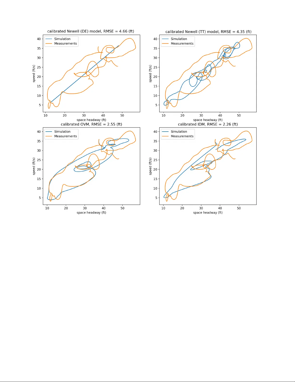
F ast Calibration of Car F ollo wing mo dels to T ra jectory data using the Adjoin t Metho d Ronan Keane Systems Engineering, Cornell Univ ersity , Email: (rlk268@cornell.edu) H. Oliv er Gao Civil and En vironmental Engineering, Cornell Univ ersit y , Email: (hg55@cornell.edu) Septem b er 22, 2020 Abstract Before a car-follo wing mo del can b e applied in practice, it m ust ﬁrst b e v alidated against real data in a process kno wn as calibration. This pap er discusses the form ulation of calibration as an optimization problem, and compares diﬀeren t algorithms for its solution. The optimization consists of an arbitrary car following mo del, p osed as either an ordinary or dela y diﬀerential equation, b eing calibrated to an arbitrary source of tra jectory data whic h may include lane changes. T ypically , the calibration problem is solved using gradien t free optimization. In this work, the gradien t of the optimization problem is deriv ed analytically using the adjoin t metho d. The computational cost of the adjoin t metho d do es not scale with the num b er of mo del parameters, which makes it more eﬃcien t than ev aluating the gradien t n umerically using ﬁnite diﬀerences. Numerical results are presented which show that quasi-newton algorithms using the adjoint metho d are signiﬁcantly faster than a genetic algorithm, and also achiev e slightly b etter accuracy of the calibrated mo del. 1 1 In tro duction 1.1 The Case for Car F ollowing and T ra jectory Data A complete traﬃc sim ulator consists of many diﬀeren t mo dules, including algorithms to determine the demand for diﬀeren t road sections, complex rules to gov ern lane changes, mergers, and diverges, a mo del to describe traﬃc ﬂow and driving b ehaviors, and more. Out of all these mo dules, the description of traﬃc ﬂo w is the most fundamen tal. The decision of what mo del is used to describ e traﬃc ﬂow has im pacts on the simulator’s strengths, weaknesses, and o verall p erformance. In particular, one imp ortan t distinction is whether to sim ulate at the macroscopic or microscopic level. A t the microscopic lev el, car follo wing models are often used. Car follo wing models describ e how a v ehicle behav es as a function of its surroundings; t ypically they are expressed as diﬀerential equations where any vehicle is coupled to the v ehicle directly ahead (i.e. its lead v ehicle). Many car follo wing models are based on common sense rules of driving. Some simple examples are adopting a sp eed based on the distance betw een y ou and y our leader, or accelerating based on the diﬀerence in speeds betw een you and y our leader. Whereas microscopic traﬃc mo dels describ e the motions of individual v ehicles, their macroscopic coun terparts treat traﬃc as a ﬂuid. At the macroscopic level, there are no vehicles, only traﬃc densities. Congested road sections with high densities slowly trickle forw ard, while uncongested traﬃc at low densities ﬂo w freely . This connection to ﬂuid dynamics was originally made b y [1], and the inﬂuence of the resulting traﬃc ﬂow theory can hardly be o verstated. In the more than six decades since, n umerous w orks ha ve attempted to improv e up on the so-called Ligh thill-Whitham-Richards (L WR) model in order to better describe v arious complex elements of traﬃc ﬂo w. Among those, [2], [3], [4], [5], [6] are p erhaps some of the most notable. Nonetheless, when it comes to macrosimulation, the L WR model, and its discrete numerical formulation ([7]), is still widely used to da y . F or all its merits, the L WR model is not without its limitations. A key relationship b et ween ﬂow and density kno wn as the “fundamental diagram”, must b e supplied. More imp ortan tly , it is assumed vehicles are homogeneous and exhibit static behavior. In real traﬃc, drivers b ehav e diﬀeren tly; vehicles hav e v arying performances; traﬃc demand ﬂuctuates; controlled intersections and lane changes hav e complex eﬀects. T raﬃc ﬂow is incredibly dynamic and inhomogeneous. The shortcomings of the L WR model become apparent in practice (see [4, 8, 9]). In the fundamen tal diagram, instead of equilibrium curves, one ﬁnds a wide scattering of p oints. The time evolution of real traﬃc ﬂow sho ws a m uch richer picture than what the L WR mo del predicts. Examining the ev olution of a v ehicle tra jectory in the sp eed-spacing plane, one sees complex hysteresis lo ops which are inconsistent with curren t macroscopic theory ([10], [11] or Fig. 2 are examples of suc h plots). Giv en these limitations, one w ould hop e for some car following mo del that could explain all these phenomena. Ho wev er, existing works are not prepared to oﬀer guidelines as to which car following mo dels are b est. It is also not clear as to ho w m uch more accurate car following mo dels are compared to macro-mo dels (like L WR). Answering either of these pressing questions is diﬃcult: the traﬃc microsimulation literature consists of literally h undreds of diﬀeren t mo dels, many of which hav e never actually b een thoroughly v alidated ([12]). W orks such as [13], [14], [15], and [16] hav e attempted to address this long-standing problem of car follo wing mo dels but hav e had v arying results as to which mo dels are best. Dra wing conclusions on the eﬃcacy of diﬀerent car follo wing mo dels requires b oth a large v ehicle tra jectory dataset (e.g. [17] or [18]) to facilitate comparison, as well as a reliable metho dology for model calibration and v alidation. The aim of this w ork is to develop new metho dology to improv e the calibration of car follo wing mo dels. Ho wev er, one should keep in mind that this only addresses one half of the c hallenge; equally imp ortan t is the creation of new datasets and new approaches for collecting accurate and meaningful traﬃc data. There is a need for an increased use of tra jectory data to study traﬃc ﬂo w. This need go es far beyond the v alidation of existing car following mo dels. As new technologies like autonomous vehicles, connected cities and on- demand mobilit y become fully realized, the L WR mo del assumption of homogeneous driv ers exhibiting static behavior b ecomes increasingly unrealistic. The limitations of macrosimulation and the uncertain ty of new tec hnology are b oth go od reasons to susp ect a growing demand for microsimulation. A t the same time, vehicle tra jectory data (which is needed for microsimulation/car following) is easier to get than ever b efore b ecause of new technologies lik e computer vision, lidar/radar, and GPS. Compared to the more commonly used lo op detector data, tra jectory data describ es traﬃc ﬂow at muc h higher temp oral and spatial resolutions. These new sources of data, still largely unexploited, can help adv ance b oth micro- and macro- theory . 1.2 Calibration Using T ra jectory Data It is relatively simple to write down some mathematical equations and call them a traﬃc mo del. F ar more diﬃcult is applying this mo del in practice. In order to v alidate a mo del against real data, one must ﬁnd the mo del parameters 2 Figure 1: On the left, an excerpt of a single lane from the NGSim data. “Incomplete” tra jectories are due to v ehicles changing to/out of the lane pictured. One can observ e man y of the imp ortan t features of traﬃc ﬂo w such as sho c kw av es, lane changing even ts, and individual driver b eha viors. Compared to macroscopic data, these features are captured at higher temp oral/spatial resolutions and without aggregation. On the right, a car following mo del (the OVM) has b een calibrated to the tra jectory data. that b est explain the data: this is kno wn as calibration. Solving the calibration problem requires b oth a dataset describing the quantit y of interest, as well as a mathematical mo del that explains the data. This pap er deals with car-follo wing mo dels that are p osed as diﬀerential equations, and may include elements suc h as dela ys, b ounds on acceleration/sp eed, and multiple driving regimes. The car-following mo del is to be calibrated against tra jectory data, time series data that describ es the motion of individual v ehicles. Existing literature has co vered v arious aspects of the tra jectory data calibration problem: the use of meta-models, sensitivit y analysis, optimization algorithms, measures of p erformance (e.g. sp eed or spacing data), and goo dness- of-ﬁt function (i.e. loss function). [19], [20], and [21] are go o d works fo cused primarily on metho dology . [22], [23], [15] and [16] are go o d works fo cused on b oth calibration and the benchmarking of v arious mo dels. In this pap er calibration is p osed as an optimization problem. F or a wide class of mo dels, b eing calibrated to tra jectory data gathered from any source, the gradient of the optimization problem has b een derived in an eﬃcient w ay using the adjoin t metho d. This enables the calibration problem to b e solved by more eﬃcien t optimization routines which use gradient information. Sev eral state of the art algorithms are b enc hmarked in order to determine b oth the accuracy of the ﬁt they can achiev e, as well as the computational eﬀort required to apply the algorithm. The pap er is organized as follo ws. Section 2 introduces car following models and discusses current researc h directions for impro ving car following mo dels. Section 3 describ es the optimization problem and discusses some issues arising in its solution. Section 4 applies the adjoin t metho d to the optimization problem and compares it to ﬁnite diﬀerences. Section 5 compares diﬀerent algorithms for solving the calibration problem. 2 Car-F ollo wing Mo dels W e will consider any car-following mo del that can b e expressed as either an ordinary or delay diﬀerential equation. This describes the ma jority of models in the literature, as w ell as the ma jorit y of mo dels used in commercial microsim ulation pack ages ([24]). W e deal with mo dels of the following form ¨ x n ( t ) = h ( ˙ x n − 1 ( t − τ ) , x n − 1 ( t − τ ) , ˙ x n ( t − τ ) , x n ( t − τ ) , p ) (1) where x n ( t ) is the p osition of vehicle n at time t . h is the car-follo wing model, whic h depends on parameters p , the “follo wing” v ehicle x n and “lead” vehicle x n − 1 . τ is a time-delay parameter which represents human reaction time. Eq. (1) states that a driver’s b eha vior (how they choose to accelerate) is determined from the sp eed and p osition of their own car, the sp eed and p osition of the leading car, and parameters p . Given a lead v ehicle tra jectory x n − 1 ( t ), 3 parameters p , and initial condition x n ( t n ), the car following mo del (1) will produce the follow er tra jectory x n ( t ). The presence of nonzero τ leads to a delay diﬀerential equation (DDE). Many car-following mo dels (including most of those used in commercial softw are) treat reaction time explicitly by using a DDE. Besides ODEs and DDEs, some car-following models are formulated as stochastic diﬀeren tial equations or derived using nonparametric techniques. W e brieﬂy discuss these types of mo dels in section 2.3 but the current metho dology do es not address their calibration. 2.1 Ordinary Diﬀerential Equations Eq. (1) giv es a general form for car-follo wing mo dels. The simplest type of mo del is a ﬁrst-order ODE where the sp eed of the following vehicle n is completely determined by the space headw ay ( x n − 1 − x n ). In this type of model, eac h driver adopts a sp eed based on the distance b et ween their car and the leading car. This simple kind of mo del is important b ecause of its connection to macroscopic theory and the L WR model. Sp eciﬁcally , if one assumes all v ehicles are identical, and in terprets the recipro cal of density as headw ay , then a functional relationship b etw een traﬃc ﬂow and density can b e recast as a relationship betw een vehicle sp eed and headw ay ([25]). Under these assumptions, the fundamen tal diagram can be though t of as describing a ﬁrst-order car-follo wing mo del. Consider the Newell car following mo del an example ˙ x n ( t ) = min { v f , x n − 1 ( t ) − x n ( t ) − s jam α } . (2) v f , α and s jam are parameters describing a triangular fundamen tal diagram ([22]). Namely v f is the speed of a v ehicle during free ﬂow, s jam is the distance b et ween tw o completely stopp ed vehicles, and − s jam /α is the sho c kwa ve sp eed. The New ell model can also be written as a tra jectory translation model, where the tra jectory of a following v ehicle is equiv alen t to the lead v ehicle tra jectory , translated o ver b oth space and time. x n ( t ) = x n − 1 ( t − α ) − s jam (3) W e refer to Eq. (3) as New ell (TT) and Eq. (2) as Newell (DE), where the acronyms stand for tra jectory translation and diﬀerential equation, resp ectiv ely . In the sp ecial case where the TT and DE mo dels b oth use a numerical time step equal to α , and vehicles are alwa ys in the congested regime (i.e. not moving at their free ﬂo w speeds), the tw o mo dels b ecome equiv alent ([25]). In this special case, either model gives tra jectories that exactly ob ey the L WR mo del with a triangular fundamental diagram. In general how ever, the t wo mo dels are diﬀeren t (see for example Fig. 2). The adv an tages of the New ell (TT) or (DE) mo dels are that they contain a small num b er of parameters, and those parameters are easily interpretable under macroscopic theory . More complicated car-following models (compared to those of New ell) are sometimes criticized for tw o main reasons: ﬁrst, for not ha ving enough empirical support for their v alidit y , and second, for ha ving too man y parameters. Despite these criticisms, more complicated mo dels ha ve b eha viors that attract researc hers. F or example, the optimal v elo cit y mo del (OVM) prop osed by [26] exhibits a sp on taneous phase transition b et ween free ﬂo w and congested states, whic h may describ e “phantom” traﬃc jams ([27]). Another example is the intelligen t driver mo del (IDM) prop osed by [28], whic h can qualitatively repro duce a num b er of complex (empirical) traﬃc states. Besides more recen t mo dels like OVM or IDM, there are also a plethora of older mo dels to complicate the mix ([12]). The default mo dels in most mo dern traﬃc sim ulator pack ages (for example, VISSIM or AIMSUN) are still older car-following mo dels ([24]), presumably b ecause it is unclear if the new er car-following mo dels oﬀer any b eneﬁts. Fig. 2 compares each of the four mo dels just men tioned by calibrating them to a single v ehicle tra jectory from the reconstructed NGSim data ([29]). The calibration minimized the ro ot mean square error (RMSE) b et ween the sim ulation and measuremen ts. The vehicle (ID 1013) was recorded for only 55 seconds, but ev en in that time man y h ysteresis lo ops w ere recorded in the sp eed-headw ay plane. F or the NGSim data, which was recorded on the freewa y in congested conditions, tra jectories that qualitatively resem ble this one are the rule rather than the exception. The diﬀeren t mo dels all give a diﬀeren t caricature of the oscillatory b eha vior observed. In particular, the Newell (TT) mo del (with a simulation time step of .1 s) app ears to b etter capture the seemingly chaotic nature of the oscillations, whereas the more complicated (and computationally exp ensiv e to calibrate) IDM or OVM mo dels result in a lo wer RMSE and b etter capture the width of the hysteresis (the diﬀerences in sp eeds at a given headwa y). The p oin t of this ﬁgure is not to make a case for one mo del ov er the other, but rather to p oin t out the interesting b eha vior shown ev en in a single short tra jectory . It also raises an imp ortan t question whic h existing researc h seems unprepared to answ er. With so many diﬀerent mo dels, each of v arying complexities, whic h ones b est describ e traﬃc ﬂow? Our work on calibration is motiv ated by this question. 4 Figure 2: F our diﬀerent car following mo dels are calibrated to a single empirical vehicle tra jectory by minimizing the ro ot mean square error b et w een sim ulation and measurements. The tra jectories are plotted in the sp eed - headw ay plane. 2.2 Dela y-Diﬀeren tial Equations Compared to ODEs, DDEs are more complicated to analyze and solve. Car-follo wing mo dels typically only consider the simplest case, where time delay (reaction time) is a constant. It seems the distinction b et w een ODEs and DDEs has been giv en limited importance in the calibration literature, even though the addition of time delay as a parameter causes extra complications. As for the literature as a whole, the eﬀect of nonzero time delay on car-following mo dels is still not fully understo o d. When studying the b eha vior of car-follo wing mo dels, one common approach is to consider a line of cars with iden tical mo del parameters on a closed lo op. In this sp ecial setting, one can ﬁnd an “equilibrium” solution where all v ehicles hav e the same sp eed and same headwa y , with zero acceleration. The equilibrium solution is contrasted with an oscillatory/perio dic solution, where the sp eed of a vehicle can oscillate in a manner reminiscent of stop-and-go or congested traﬃc. Since most analytic (i.e. not numerical) results come from studying the b eha vior around the equilibrium solution, the stabilit y of the equilibrium solution is particularly important. Adjusting parameters in a model can b e said to hav e a stabilizing (destabilizing) eﬀect if the equilibrium solution will p ersist (degenerate) under a wider v ariety of conditions. Intuitiv ely , one expects that driv ers ha ving slow er reaction times will ha ve a destabilizing eﬀect, and this seems to be generally correct. It has b een sho wn for both the optimal v elo cit y mo del (OVM) and intelligen t driv er mo del (IDM) that the inclusion of time delays has a destabilizing eﬀect (see [30], [31], [32]). But time delay is not the only model parameter 5 that can hav e such eﬀects. F or example, [33] show ed that increasing (decreasing) the OVM’s “sensitivity parameter” has stabilizing (destabilizing) eﬀects (the sensitivity parameter is prop ortional to how strongly the driv er accelerates). Time delay can also hav e more subtle eﬀects: [31] found the inclusion of time dela ys for OVM caused bistability b et w een equilibrium and oscillatory solutions. In [34] the OVM is considered with diﬀeren t reaction times ≤ 0 . 3 seconds. In this range, no qualitativ e c hanges to the mo del are observ ed. The authors state that c hanging the sensitivity parameter can account for the eﬀects of reaction time. [23] and [30] ha ve done exp erimen ts on OVM with larger reaction times ( ≈ 1 seconds) and found that while it is true that reaction time is not esp ecially imp ortan t at lo w v alues, once increased past some threshold it will start to cause unstable b ehavior leading to vehicle collisions. A similar b ehavior was found in [35] for the Gipps car-follo wing mo del. These ﬁndings show the inclusion of reaction time will hav e a destabilizing eﬀect, but large reaction times seem to hav e esp ecially unstable eﬀects, p erhaps owing to some sort of phase transition. In practice, one can observ e that calibrated v alues for reaction time greatly v ary across the literature, even for the same mo del. Consider that [36],[15], and [16] all calibrate the Gipps mo del, but all ﬁnd very diﬀerent means and v ariances for driv ers’ reaction times. One found the mean to be 0.57 s with a v ariance of 0.02 s. Another found the mean to b e 1.73 s with v ariance 1.35 s. Besides reaction time, another interesting extension to a model is the inclusion of “anticipation” eﬀects. Examples of anticipation are a driver estimating the future sp eed/position of a leading vehicle, or a follo wing vehicle reacting to multiple vehicles instead of just its leader. [32] show ed that anticipation has a stabilizing eﬀect for IDM, and [37] show ed the same for OVM. Of course, due to nonlinearities, stabilizing and destabilizing eﬀects will not simply cancel out. 2.3 Sto c hastic and Data-Driv en Models In this pap er we consider the calibration of car following mo dels form ulated as ODEs or DDEs. This section dis- cusses some recen t researc h directions in whic h car follo wing models are formulated as sto c hastic diﬀeren tial equations (SDEs), or derived from data using nonparametric mo dels. P ap ers using SDEs to model traﬃc ﬂow t ypically argue that the sto c hastic mo dels are b etter able to describ e the formation and growth of congestion. Besides b eing able to ac hieve a closer ﬁt to data, authors hav e concluded that deterministic mo dels cannot repro duce some qualitative features of congestion. In particular, some recent ﬁeld exp erimen ts inv olving 25 and 51 h uman driven vehicles on a straight road ([38]) show ed that the standard deviation of traﬃc sp eeds initially grow in a concav e w ay , whereas deterministic mo dels seem to only b e able to show conv ex gro wth. SDEs in the literature are usually based on modifying an existing deterministic ODE model rather than created as an en tirely no vel mo del. Two common sto c hastic mechanisms are acceleration noise, and action p oin ts. F or acceleration noise, white noise is added to the output of the deterministic mo del. The white noise may b e sampled from either a uniform or normal distribution. Closely related to acceleration noise, is the case where the noise is added to a mo del parameter instead of directly to the output of the mo del. In [39] and [40] gaussian acceleration noise w as added to the Newell mo del and IDM resp ectiv ely . In 2D-IDM from [41] uniform noise is added to a mo del parameter (in that case, the desired time headwa y parameter). Action p oin ts are implemented by creating a mo del regime where the driver is insensitive to changes in the headwa y and/or lead vehicle velocity . Th us when inside the regime, a driver will maintain their current b eha vior un til a suﬃ- cien tly large diﬀerence in the state is achiev ed, at which p oin t the driver will react to the now signiﬁcantly diﬀerent driving situation. The reader is referred to [42] or [43] for speciﬁc details on implementing action p oin ts. The motiv ation for including white noise is to mo del random human b eha vior and reﬂect the fact that h umans can- not p erfectly control their v ehicles, whereas the motiv ation for action p oin ts is that drivers are not able to perceive min ute c hanges to the traﬃc situation and thus a suﬃcien tly large diﬀerence is required before they can start to react. [42] shows that action points and white noise hav e similar eﬀects on traﬃc sim ulations, and suggests that b oth mec hanisms should be included. Data-driv en car follo wing models are based on mac hine learning models and algorithms, and as a result their form ula- tion is signiﬁcantly diﬀeren t than the ODE/DDE/SDE discussed so far. How ever, despite their diﬀerent form ulation, the inputs (current headwa y , follow er and leader velocities) and output (curren t follow er acceleration) are typically v ery similar. Papers in the literature hav e rep orted that data-driv en mo dels can achiev e b etter ﬁts to empirical data compared to parametric mo dels such as O VM or IDM. The discussion of these mac hine learning techniques is outside the scop e of this pap er but w e mention the diﬀerent approac hes which ha ve b een successfully applied. In [44] k -nearest neighbor (knn) is used, and [45] uses locally weigh ted regression (lo ess), which can b e thought of as a generalization of knn. [46] discuss using feedforward neural netw orks with a single hidden lay er and ReLU nonlinear- 6 it y . That pap er also uses recurren t neural netw orks (RNNs) to ov ercome some diﬃculties of the feedforward neural net works. [47] uses long short-term memory neural netw orks, a sp ecial kind of RNN. [48] use deep reinforcement learning (deep RL) and p olicy gradients, and do a comparison b etw een deep RL, IDM, RNN, lo ess, and feedforward neural netw orks. 3 Calibration It is useful to rewrite the second order diﬀerential equation Eq. (1) as a system of ﬁrst order equations: ˙ x n ( t ) =  ˙ x ∗ n ( t ) ˙ v n ( t )  =  v n ( t ) h ∗ ( x n − 1 ( t − τ n ) , x n ( t − τ n ) , p n )  = h n ( x n ( t ) , x n ( t − τ n ) , x L ( n ) ( t − τ n ) , p n ) (4) where x n is now a vector consisting of the p osition and velocity of vehicle n at time t . x ∗ n and v n refer to the p osition and speed for v ehicle n . p n denotes the parameters for v ehicle n . L ( n, t ) refers to the leader of v ehicle n at time t , and w e denote the lead tra jectory as x L ( n ) (time dep endence suppressed) to reﬂect the fact that the index corresp onding to the lead vehicle may change due to lane changing. Eq. (4) is what we refer to when we sa y “car-following mo del” and its solution x i ( t ) is a “simulated tra jectory”. The calibration is done for some arbitrarily sized plato on of n vehicles, indexed as 1 , . . . , n . Each vehicle has some individual parameters p i and a corresp onding car follo wing mo del h i , so all vehicles ha ve their o wn set of parameters, and p i only describ es vehicle i . Let p be a concatenated v ector of all the parameters, so p = [ p 1 , p 2 , . . . , p n ]. Calibration ﬁnds the parameters p which minimize the total loss b etw een the sim ulated tra jectories x i ( t ) and the corresp onding measured vehicle tra jectories, which are denoted ˆ x i ( t ). The loss function is denoted as f ( x i , ˆ x i , t ) and represen ts the goo dness of ﬁt of the simulated tra jectory x i at time t . The measurements ˆ x i ( t ) are known in the in terv al [ t i , T i ] for each i . In order to compute the simulated tra jectories for each vehicle i , we require a lead vehicle tra jectory x L ( i ) ( t ) as well as an initial condition x i ( t i ). The time in terv al that the lead vehicle tra jectory is known is denoted [ t i , T i − 1 ]. x i ( t i ) is the initial condition, which is speciﬁed as x i ( t i ) = ˆ x i ( t i ) for an ODE mo del. F or an ODE, the optimization problem is min p F = n X i =1 Z T i − 1 t i f ( x i , ˆ x i , t ) dt (5) s.t. ˙ x i ( t ) − h i ( x i ( t ) , x L ( i ) ( t ) , p i ) = 0 , t ∈ [ t i , T i − 1 ] , i = 1 , . . . , n x i ( t i ) − ˆ x i ( t i ) = 0 i = 1 , . . . , n b low ≤ p ≤ b high The ob jective function F is deﬁned as the in tegral of the loss function f o ver time, summed ov er each simulated v ehicle. The constraints are that the sim ulated tra jectories x i ob ey the car-following mo del h i from time t i to T i − 1 , with the initial conditions x i ( t i ) = ˆ x i ( t i ). There may also b e some b o x constraints b low , b high whic h preven t parameters from reaching unrealistic v alues. The DDE case is similarly deﬁned: min p F = n X i =1 Z T ∗ i − 1 t i + τ i f ( x i , ˆ x i , t ) dt (6) s.t. ˙ x i ( t ) − h i ( x i ( t ) , x i ( t − τ i ) , x L ( i ) ( t − τ i ) , p i ) = 0 , t ∈ [ t i + τ i , T ∗ i − 1 ] , i = 1 , . . . , n x i ( t ) − ˆ x i ( t ) = 0 t ∈ [ t i , t i + τ i ] , i = 1 , . . . , n b low ≤ p ≤ b high where T ∗ i − 1 = min { T i − 1 + τ i , T i } , and the reaction time for v ehicle i , τ i , is assumed to be a mo del parameter. x i ( t ) − ˆ x i ( t ) = 0 deﬁnes the history function for x i (DDEs hav e history functions as their initial conditions). 3.1 Do wnstream Boundary Conditions for Car F ollo wing Mo dels In Eqs. (5) and (6) w e ha v e speciﬁed the initial conditions, whic h giv e the times v ehicles en ter the simu lation and their p osition/speed upon entering. These conditions migh t also b e referred to as upstream boundary conditions since they state how vehicles en ter the simulation. F or video data such as NGSim, which is recorded on a ﬁxed section of road, do wnstream boundary conditions also need to b e sp eciﬁed. Video data has staggered observ ation times ( T i − 1 < T i ) 7 meaning that a v ehicle’s leader leav es the study area before the vehicle itself. Figure 3 gives a visual depiction of this. 2 𝐿 ( 1 ) 1 Dir ec tion of tr a v el End of simula tion 2 1 Dir ec tion of tr a v el End of simula tion Figure 3: Boxes represen t v ehicles; v ehicle 2 follows 1, and 1 follows L (1). In top panel, the leader L (1) is still in the sim ulation and so the car following mo del can b e used to up date v ehicle 1. In b ottom panel, L (1) is no longer in the simulation, and so a do wnstream b oundary condition is used to up date vehicle 1. Car following mo dels require a lead vehicle tra jectory as input, therefore once the lead v ehicle lea ves the simulation, the car follo wing model can no longer b e used. Downstream b oundary conditions then give a rule for the dynamics a vehicle follows once its lead vehicle leav es the sim ulation (i.e. they sp ecify the dynamics for x i ( t ) , t ∈ [ T i − 1 , T i ]). The the b oundary conditions w e implement in this paper are ˙ x i ( t ) = ˙ ˆ x i ( t ) , t ∈ [ T i − 1 , T i ] (7) meaning that when a vehicle’s leader is no longer av ailable, the vehicle will mov e with whatever sp eed was recorded in the data. Under these b oundary conditions, the velocity v i ( t ) and acceleration ˙ v i ( t ) will b e piecewise contin uous (they will hav e a jump discontin uity at T i − 1 ). The ob jective F and gradient dF /dp are still contin uous under this b oundary condition (see sections 3.3 and 4.1.2 for the relev ant discussion on discontin uities in car following mo dels and how they impact the calibration problem). Note that for a DDE, the time T ∗ i − 1 is used instead of T i − 1 . It is necessary to specify the downstream b oundary conditions for tw o reasons. First, it allows vehicles to exit the sim ulation area. Second, it allows congestion to prop ogate into the simulation area from do wnstream. This happ ens when the b oundary conditions specify a reduction in sp eed. 3.2 Reaction Time as a P arameter Sim ulated tra jectories are computed n umerically with a speciﬁed time discretization. Since we wan t to compare the sim ulated tra jectories with the actual measurements, it mak es sense for the sim ulation to use the same time discretization as the data. F or example, if the data is recorded every 0.1 seconds, the simulated tra jectories should use a time step of 0.1 seconds. If the sim ulation used a diﬀerent time step (e.g. 0.09), then the loss can only b e calculated at a few p oin ts (e.g. 0.9, 1.8) unless we deﬁne some in terp olation pro cedure. F or a DDE, the time discretization and reaction time need to be multiples of each other. If the simulation uses a time step of 0.1 seconds, then the reaction time will ha ve to b e an integer multiple of 0.1 (e.g. 0.1, 0.2). W e can either: 1. Enforce that every vehicle’s reaction time is a in teger multiple of 0.1 2. Allo w reaction time to b e a contin uous v ariable and deﬁne the loss function through interpolation. If we choose 1, it leads to a mixed in teger nonlinear programming problem (MINLP). This is a muc h harder problem than the original nonlinear program. One approach used in [16] would b e to split up all vehicles into small plato ons (either pairs or triplets) and use a brute force searc h for reaction time. Ho w ever, ev en when the plato ons are small, using brute force v astly increases computation b ecause the calibration has to be rep eated for every possible com bination of reaction times. 8 The other option is to use an approach similar to [23] where reaction time is a contin uous v ariable and in terp olation is used on the simulated tra jectories. In general, an y sort of interpolation could b e used, but linear in terp olation is the most common. In this approac h, in terp olation needs to b e used on the lead tra jectory and initial history function in order to deﬁne the mo del. Assuming the n umerical time step is not equal to the dela y , in terp olation will need to b e used on the sim ulated tra jectory as well. One issue with interpolation is how to compute the loss function. Speciﬁcally , assuming the simulation is deﬁned on a diﬀerent set of times than the measurements, should the simulation b e interpolated onto the measurement’s times or vice versa? W e suggest doing b oth. This av oids the p ossibilit y of error cancelation occurring during the in terp olation and causing the loss function to b e erroneously small. In this scenario it w ould be preferable to rew eight the loss function as well since the loss will b e computed ov er more p oin ts. 3.3 Multiple Regimes, Lane Changing, and Discontin uities in Car F ollo wing Mo dels W e say a mo del has multiple regimes when the mo del is expressed either as a piecewise function, or b y using min and max functions. These types of mo diﬁcations are frequently applied in practice. P erhaps the most common are examples like Eq. (2), where the maximum sp eed is explicitly constrained b y some constant v f . F or second order mo dels, often the acceleration will b e constrained b et ween minim um and maximum accelerations a min , a max . Besides these simpler regimes which implement b ounds on the acceleration and/or velocity , there are also mo dels which use diﬀeren t regimes to describ e diﬀerent car following b eha vior. The Gipps mo del ([49]) is one suc h example, which has one regime to describe normal car follo wing b eha vior, and a second regime whic h implements an emergency braking b eha vior. Other examples of multi-regime mo dels are the constan t acceleration heuristic prop osed in [50], the follow er stopp er controller prop osed in [51], or any mo del implementing action p oin ts. W e consider h i ( x i , x L ( i ) , p i ) = ( h i, 2 g i, 2 ( x i , x L ( i ) , p i ) ≥ 0 h i, 1 otherwise (8) as a general form of a tw o regime car follo wing mo del, with the tw o regimes h i, 1 and h i, 2 . The condition for the asso ciated regime to b ecome activ ated is g i, 2 (whic h is p ossibly a vector v alued function). F or example with Eq. (2): h i, 1 = ( x L ( n ) − x n − s jam ) /α , h i, 2 = v f and g i, 2 = h i, 1 − h i, 2 . There must alwa ys b e m − 1 such conditions for a mo del with m regimes, so a model with more regimes will simply hav e h i, 2 , . . . , h i,m and g i, 2 , . . . , g i,m . In the case of a ﬁrst order mo del’s velocity being b ounded, or a second order mo del’s acceleration b eing b ounded, the resulting mo del h i is everywhere contin uous (b ecause b oth regimes will b e equal when the switching condition g i, 2 is met). In general a multi-regime mo del need not b e everywhere contin uous. Gipps and follow er stopp er are b oth examples of a multi-regime mo del b eing ev erywhere contin uous; the constant acceleration heuristic or a mo del implemen ting action points are examples not guaren teed to be con tinuous when switc hing betw een regimes. Of course, even for a m ulti-regime mo del which is everywhere contin uous, its deriv ativ es will hav e discontin uities when switc hing b et ween regimes. Note that a m ulti-regime mo del written using min and max will alwa ys b e contin uous. The reason why we prefer using the form Eq. (8) is b ecause 1) it is more general, 2) w e can explicitly refer to the switc hing condition g i, 2 and 3) the regime of the mo del is explicitly stated, which av oids the problem of the regime b eing ambiguous when the quantities inside a min / max are equal. Lane changing is another issue which causes discon tinuities in car following models. Sp eciﬁcally , whenever a lead v ehicle c hanges, i.e. L ( i, t ) c hanges, then the lead v ehicle tra jectory x L ( i ) will hav e a jump discontin uity , and therefore h i will hav e a jump discontin uit y as w ell. Giv en that lane changing alwa ys causes discontin uities and multi-regime mo dels may cause discontin uities, one ma y w orry whether or not the ob jective F will hav e discon tinuities, and whether or not the gradien t dF /dp is even guaren teed to exist. W e give suﬃcient conditions for the contin uit y of F and dF /dp in section 4.1.2. 3.4 Algorithms for Solving the Calibration Problem Eqs. (5) and (6) are nonlinear and non-conv ex optimization problems that must b e solved numerically . Curren t approac hes usually rely on gradient-free optimization, with genetic algorithm (GA) and Nelder-Mead simplex algo- rithm (NM) b eing the tw o most commonly applied algorithms ([12, 52, 13, 14, 53, 23, 15, 16]). These metho ds hav e the disadv antage of being slo w to conv erge, and require many ob jectiv e function ev aluations. The ob jective F is relativ ely expensive to compute in this context b ecause w e ﬁrst must solve a system of diﬀerential equations (i.e. compute the sim ulated tra jectories). As an alternative to directly solving the optimization problems (5) and (6), parameters can b e estimated directly from data using statistics techniques ([54, 55, 56, 57]) but this approach is not guaran teed to ﬁnd lo cal minima. Also, mo dels ma y hav e parameters whic h do not ha ve clear physical interpretations, and therefore cannot b e directly estimated. 9 Gradien t-based optimization algorithms can p oten tially solv e the calibration problem faster than gradien t-free approac hes. How ever, even though most optimization algorithms use gradient information, not many gradien t-based algorithms ha ve b een examined in the calibration literature. T o the authors’ kno wledge, the only gradien t-based algorithms that hav e b een considered are simultaneous p erturbation stochastic appro ximation (SPSA) (see [58]), Lindo’s Multistart (a commercial solver’s global optimization routine, see [59]), and sequential quadratic programming using ﬁltering (SQP-ﬁlter, see [60]). In [61] SQP-ﬁlter was found to give better solutions than NM or GA, as well as solve the problem up to 10 times faster; even b etter results were found when it was additionally combined with gradient-free algorithm DIRECT ([62]). [35] did not consider computational sp eed, but found the Multistart algorithm had a muc h higher chance of ﬁnding the true global minim um compared to GA or NM. Ev en if one only knows ho w to explicitly ev aluate the ob jective function F , it is not necessary to use gradient-free optimization b ecause the gradien t (the vector dF /dp ) can be calculated numerically . T o do this, one v aries the parameters p one at a time, and recomputes the ob jectiv e each time a parameter is v aried. Then the gradien t can b e calculated using ﬁnite diﬀerences. W e refer to this as the ﬁnite diﬀerence approach for computing the gradien t, and it requires us to recompute the sim ulated tra jectories of every single vehicle m additional times, where m is the n umber of parameters. When using a forward euler scheme with stepsize ∆ t for an ODE mo del, the computation cost for computing the simulated tra jectories once is O ( T ( n )), where T ( n ) = P n i =1 ( T i − 1 − t i ) / ∆ t . So computing the gradien t with ﬁnite diﬀerences has a complexity of O ( mT ( n )). The adjoint metho d has complexity O ( T ( n )), and so it is the prefered metho d for computing the gradient when m is large ([63, 64]). 4 Adjoin t Metho d and Gradien t-Based Optimization In this pap er we are primarily concerned with applying the adjoint metho d to Eq. (5) in order to eﬃciently ev aluate the gradient dF /dp for an ODE mo del. The gradient can then b e used with an y gradien t-based optimization routine. In this section we deriv e the gradient and compare it to using ﬁnite diﬀerences; we consider diﬀerent optimization algorithms in the next section. The adjoint metho d can also b e applied to the calibration problem (6) where the mo del includes time delay . It can also b e used to calculate the hessian. Both of these extensions follow the same techniques elab orated in this section, and are included in the app endix. W e ﬁrst consider the calibration of a single vehicle ( n = 1) b efore dealing with the general case of an arbitrary n umber of v ehicles. 4.1 Adjoin t Method for ODEs In our notation, x i , h i , and p are vectors, and f and F are scalars. A deriv ativ e of a scalar with resp ect to a v ector is a vector, so for example ∂ f /∂ x i = [ ∂ f /∂ x ∗ i , ∂ f /∂ v i ]. A deriv ative of a vector with resp ect to a vector is a matrix, where the rows corresp ond to the vector b eing diﬀerentiated, and the columns corresp ond to the vector b eing diﬀerentiated with resp ect to. F or example, ∂ x i ∂ p =  ∂ x ∗ i /∂ p 1 ∂ x ∗ i /∂ p 2 . . . ∂ x ∗ i /∂ p m ∂ v i /∂ p 1 ∂ v i /∂ p 2 . . . ∂ v i /∂ p m  where p j represen ts the j th parameter. Additionally , the sup erscript T indicates transp ose. Deﬁne the augmented ob jective function, denoted L L = Z T n − 1 t n dt  f ( x n , ˆ x n , t ) + λ T ( t )  ˙ x n ( t ) − h n ( x n ( t ) , x L ( n ) ( t ) , p n )   (9) in this equation, λ ( t ) is referred to as the adjoin t v ariable. λ ( t ) has the same dimension as the state v ariable x n ( t ), so it is a length tw o vector for a second order mo del. Note that since ˙ x n − h n ( · ) = 0, we hav e that L = F . These equalities are alwa ys true regardless of the choice of λ ( t ). F ollowing the observ ation that L = F , it follows that dL/dp = dF /dp , so diﬀerentiating Eq. (9) with resp ect to the parameters p gives d dp F = d dp L = Z T n − 1 t n dt  ∂ f ∂ x n ∂ x n ∂ p + λ T ( t )  ∂ ˙ x n ∂ p − ∂ h n ∂ x n ∂ x n ∂ p − ∂ h n ∂ p  (10) where quantities are ev aluated at time t if not explicitly stated. Note in this case there are no terms dep ending on the lead tra jectory x L ( n ) since the plato on consists only of x n and the lead tra jectory is regarded as ﬁxed. 10 Eq. (10) cannot b e computed in the current form b ecause we hav e no wa y to calculate ∂ x n /∂ p . The adjoint metho d w orks by choosing the the adjoint v ariable λ ( t ) in a wa y whic h allows us to a void the computation of the unkno wn ∂ x n /∂ p . When doing this, one will ﬁnd that the correct choice of λ ( t ) results in solving a similar system to the original constrain t, but “backw ards” (e.g. when the mo del is an ODE, λ ( t ) will end up b eing deﬁned as an ODE whic h is solved bac kwards in time). The equations whic h deﬁne the adjoint v ariable are kno wn as the adjoint system. T o derive the adjoint system, ﬁrst apply integration b y parts: Z T n − 1 t n λ T ( t ) ∂ ˙ x n ∂ p dt = λ T ( t ) ∂ x n ∂ p     T n − 1 t n − Z T n − 1 t n ˙ λ T ( t ) ∂ x n ∂ p dt (11) The quantit y ∂ x n ( t n ) /∂ p is known because it simply dep ends on the initial conditions; based on (5) it is simply zero. W e will choose λ ( T n − 1 ) = 0 to eliminate the ∂ x n ( T n − 1 ) /∂ p term. This choice b ecomes the initial conditions for the adjoin t system; note that L = F regardless of ho w the initial conditions for λ are chosen. Now combining Eqs. (10) and (11): d dp F = Z T n − 1 t n dt   ∂ f ∂ x n − ˙ λ T ( t ) − λ T ( t ) ∂ h n ∂ x n  ∂ x n ∂ p − λ T ( t ) ∂ h n ∂ p  Then to av oid calculating ∂ x n /∂ p we will enforce: ∂ f ∂ x n − ˙ λ T ( t ) − λ T ( t ) ∂ h n ∂ x n = 0 , t ∈ [ T n − 1 , t n ] (12) Eq. (12) deﬁnes a new diﬀeren tial equation in λ ( t ). Our choice λ ( T n − 1 ) = 0 is the corresp onding initial condition. Then after solving for λ ( t ) we can calculate the desired gradient: d dp F = − Z T n − 1 t n λ T ( t ) ∂ h n ∂ p dt (13) 4.1.1 N Car Plato on No w we will apply the adjoint metho d to a platoon of arbitrary size, and sketc h a general algorithm for computing the gradient. Deﬁne the augmented ob jective function and pro ceed as b efore. Again, we suppress t dep endence for clarit y . L = n X i =1 Z T i − 1 t i f ( x i , ˆ x i ) + λ T i  ˙ x i − h i ( x i , x L ( i ) , p i )  dt + Z T i T i − 1 λ T i ( ˙ x i − ˙ ˆ x i ) dt ! (14) d dp F = d dp L = n X i =1 Z T i − 1 t i ∂ f ∂ x i ∂ x i ∂ p − λ T i ( t ) ∂ h i ∂ x i ∂ x i ∂ p − λ T i ( t ) ∂ h i ∂ p dt ! + n X i =1 Z T i t i λ T i ( t ) ∂ ˙ x i ∂ p − 1 ( G ( i, t ) 6 = 0) λ T G ( i ) ( t ) ∂ h G ( i ) ∂ x i ∂ x i ∂ p dt ! Here, λ n corresp onds to the adjoint v ariables for v ehicle n . Similar to ho w L ( n, t ) was deﬁned, G ( n, t ) is deﬁned as the index of v ehicle n ’s follow er at time t , so that x G ( n ) is the follo wing tra jectory of vehicle n . If vehicle n has no follow er at time t , or if the fol lower is not p art of the plato on b eing c alibr ate d , let G ( n, t ) return zero. 1 is the indicator function. When n > 1, the downstream b oundary conditions m ust b e put into the augmented ob jective function, b ecause a vehicle i may aﬀect its follow er in the time [ T i − 1 , T i ], even though it only contributes to the loss function during [ t i , T i − 1 ]. Apply in tegration by parts, tak e the initial condition as λ i ( T i ) = 0, and gather terms with ∂ x i /∂ p to form the adjoin t system: − ˙ λ T i ( t ) + 1 ( t ≤ T i − 1 )  ∂ f ∂ x i − λ T i ( t ) ∂ h i ∂ x i  − 1 ( G ( i, t ) 6 = 0) λ T G ( i ) ( t ) ∂ h G ( i ) ∂ x i = 0 , t ∈ [ T i , t i ] , ∀ i (15) Comparing this adjoint system to the one for a single vehicle (12), the diﬀerence here is that there is an extra con tribution which occurs from the coupling b et ween vehicles. This coupling term o ccurs only when a v ehicle acts as a leader for another vehicle in the same plato on. After solving the adjoin t system, d dp F = n X i =1 − Z T i − 1 t i λ T i ( t ) ∂ h i ∂ p dt ! (16) 11 All the partial deriv ativ es in Eqs. (15) , (16) are computed exactly for a given loss function and car-following mo del. Solving for x i ( t ) , λ i ( t ) , and dF /dp is done numerically with an appropriate time discretization. The same discretiza- tion should b e used for all quan tities, so if one uses a forward euler scheme for x i , the same forward euler scheme should b e used for λ i and the integral in F should use a left Riemann sum. Note as well that for a multi-regime mo del, one should keep the regime for each timestep in memory , b ecause otherwise the switching condition g i,n will ha ve to be ev aluated at each timestep when computing the adjoin t v ariables. W e deﬁne a general algorithm for computing F , d dp F : Inputs: measured tra jectory data ˆ x 1 ( t ) , . . . , ˆ x n ( t ), an y necessary lead vehicle tra jectories x L ( i ) ( t ) for i ∈ [1 , . . . , n ] , L ( i, t ) / ∈ [1 , . . . , n ]. Models h 1 , . . . , h n with parameters p 1 , . . . , p n . 1. F or each vehicle i ∈ [1 , . . . , n ]: (a) Compute simulated tra jectory x i ( t ), t ∈ [ t i , T i − 1 ] b y solving ˙ x i ( t ) = h i ( x i , x L ( i ) , p i ) with intial condition x i ( t i ) = ˆ x i ( t i ). (b) Compute x i ( t ), t ∈ [ T i − 1 , T i ] using downstream b oundary conditions Eq. (7) (c) Keep in memory: x i ( t ), G ( i, t ), and the regime of h i at each time 2. Compute ob jective F = P n i R T i − 1 t i f ( x i , ˆ x i , t ) dt 3. F or eac h adjoin t v ariable i ∈ [ n, . . . , 1] : compute λ i ( t ), t ∈ [ T i , t i ] by solving adjoin t system Eq. (15) with initial condition λ i ( T i ) = 0. 4. Compute gradient dF /dp = − P n i R T i − 1 t i λ T i ∂ h i /∂ p dt Outputs: F , dF /dp 4.1.2 Suﬃcien t Conditions for a Contin uous Ob jectiv e and Gradien t Theorem 1. The fol lowing ar e suﬃcient c onditions for F and dF /dp to b e c ontinuous: 1. the loss function f ( x i , ˆ x i ) and its p artial derivative ∂ f /∂ x i ar e pie c ewise c ontinuous on [ t i , T i − 1 ] for al l i 2. the c ar fol lowing mo del h i ( x i , x L ( i ) , p i ) and its p artial derivatives ∂ h i /∂ x i , ∂ h i /∂ p , and ∂ h i /∂ x L ( i ) ar e pie c ewise c ontinuous on [ t i , T i − 1 ] for al l i 3. ∂ h i /∂ x i must b e able to b e b ounde d by a c onstant 4. for a multi-r e gime mo del, the Eq. 17 must b e satisﬁe d wher e it is additional ly assume d that x L ( i ) ( t ) , L ( i, t ) / ∈ [1 , . . . , n ] (any le ad vehicle tr aje ctories which ar e r e quir e d but not simulate d) ar e pie c ewise c ontinuous and ˆ x i ( t ) , i ∈ [1 , . . . , n ] ar e c ontinuous. Corollary 1. If in addition to F and dF /dp b eing c ontinuous, ∂ f /∂ x i , ∂ h i /∂ x L ( i ) , and ∂ h i /∂ p ar e b ounde d, then F is Lipschitz c ontinuous. W e conclude that a m ulti-regime model need not be con tin uous when switching b et ween regimes, and lane c hanging, whic h will alwa ys cause jump discon tinuities in h i ( x i , x L ( i ) , p i ), is allo wed. Note that by piecewise contin uity w e mean a mo del (or loss function) can switch regimes only a ﬁnite num b er of times in a ﬁnite time interv al (and eac h regime is con tinuous); additionally , the time interv al of each regime must b e contin uous with resp ect to the mo del parameters. Refer to the the full pro of in the app endix for further details. W e also show in the app endix that the ob jective is Lipschitz contin uous for the OVM, which was the mo del used for the numerical exp erimen ts in this pap er. 4.2 Implemen tation of Adjoin t Metho d and Calibration Problem T o test the adjoint method and optimization algorithms, the calibration problem Eq. (5) was implemen ted in python for the optimal velocity mo del. The equations b elo w show the functional form of the mo del as originally formulated in [57] and [26]. ¨ x n ( t ) = c 4 ( V ( s ) − ˙ x n ( t )) V ( s ) = c 1 [tanh( c 2 s − c 3 − c 5 ) − tanh( − c 3 )] 12 c 1 through c 5 are the 5 parameters of the mo del. s is the space headw ay , deﬁned as s = x L ( i ) − x i − l L ( i ) , where l i is the length of vehicle i . All vehicles ha ve their o wn unique parameters, so the total num b er of parameters in the optimization problem is 5 times the n umber of vehicles. The optimal velocity mo del and its adjoint system were b oth discretized with a forw ard euler scheme. The data used was the reconstructed NGSim data ([29]), so a time step of .1 seconds was used to b e consistent with this data. The loss function f used was square error, which w as discretized with a left Riemann sum. f ( x i , ˆ x i , t ) = ( x ∗ i ( t ) − ˆ x ∗ i ( t )) 2 F = n X i =1 T i − 1 X t = t i f ( x i , ˆ x i , t ) whic h is equiv alen t to minimizing the ro ot mean square error (RMSE) RMSE = s F P n i =1 T i − 1 − t i Since only a car following mo del is b eing calibrated, any lane c hanges in the measurements will be the same lane c hanges in the simulation. This also means that the leader/follo wer relationships in the simulation are the same as they are in the data. This allo ws tra jectories to be calibrated at the lev el of individual v ehicles, since it does not mak e sense to directly compare the simulated and measured tra jectories of a vehicle if the simulation and measurements ha ve diﬀerent lead v ehicles. 4.3 Adjoin t method compared to other metho ds for calculating the gradien t Man y optimization algorithms will automatically use ﬁnite diﬀerences to compute the gradient if an explicit gradient function is not given. Sim ultaneous p erturbation is another option when using an optimization algorithm like the one outlined in [58]. Then, assuming that one has c hosen to use a gradient-based algorithm for calibration, it is of practical interest to inv estigate ho w the adjoin t metho d compares to b oth of these metho ds. Speciﬁcally , how do es the sp eed and accuracy of these three metho ds compare in practice? 4.3.1 Comparison of Sp eed The computational cost of an ob jectiv e function ev aluation is O ( T ( n )), where T ( n ) is the n um b er of simulated timesteps, added ov er all n vehicles. The theoretical computational complexities for the adjoin t metho d is O ( T ( n )), while forward diﬀerences has O ( mT ( n )), where m is the num b er of parameters. The sim ultaneous p erturbation metho d has O ( kT ( n )) complexit y , where the ﬁnal gradien t is the a verage of k estimates of the gradient. Note that these computational complexities are only for the gradien t calculation and do not consider the complexit y of whatever optimization algorithm the gradient is used with. T o test these theoretical results in practice, the gradien t of the calibration problem w as calculated and the platoon size w as v aried. Since the OVM was used, the total num b er of parameters is 5 times the n umber of vehicles. W e considered a plato on having b etw een 1 and 15 vehicles. The results are shown in the ﬁgure 4. Figure 4’s left panel shows the total CPU time, measured in seconds, needed to calculate the gradient of the calibration problem using the three diﬀerent metho ds. The sim ultaneous perturbation w as done with both 1 and 3 trials, denoted SPSA and SPSA-3. The right panel sho ws the time needed to calculate the gradient divided by the time needed to calculate the ob jective. T o minimize the randomness in the CPU times, eac h data p oin t w as repeated 10 times and the results were av eraged. Some v ariation is still present b ecause some vehicles are observed for shorter times. The same 15 vehicles were used in the exp erimen t and alwa ys added in the same order. It should also b e stated that for either a ﬁnite diﬀerencing scheme or for the adjoint metho d, one nee ds to ﬁrst compute the ob jective b efore computing the gradien t. Therefore, it should b e implicitly understo od that “time to calculate the gradien t”, really refers to “time to calculate b oth the ob jective and gradien t” for those t wo metho ds. This sho ws that using a ﬁnite diﬀerence metho d quic kly b ecomes in tractable when the num b er of parameters increases. The time increases quadratically in the left panel b ecause b oth m and T ( n ) are increasing. In the right panel, when the time needed to calculate the gradient is divided b y the time needed to calculate the ob jectiv e, one sees the complexity growing as a linear function of m . In that ﬁgure, we also see that the complexities for the adjoint metho d and simultaneous p erturbation do not dep end on m . The table 1 sho ws the cpu times for 5-15 parameters. One can observe that this implementation of the adjoint metho d for OVM requires the equiv alen t of 4 ob jectiv e function solves, whereas forw ard diﬀerences requires m + 1 (where there are m parameters). 13 Figure 4: Time for a single ev aluation of the gradien t for a progressively larger calibration problem. The ob jective v aried from the loss from a single vehicle (5 parameters) to 15 vehicles (75 parameters). T able 1: T able of sp eeds for adjoint metho d compared to ﬁnite diﬀerences for computing the gradient. Relativ e time refers to the equiv alent num b er of ob jectiv e function ev aluations. P arameters Ob j. time (s) Adjoin t time (s) Adjoin t relativ e time Finite time (s) Finite relative time 5 .0062 .0250 4.03 .0390 6.3 10 .0109 .0438 4.02 .1250 11.5 15 .0172 .0686 3.99 .2811 16.3 4.3.2 Comparison of Accuracy F or the calibration problem, there is no wa y to calculate the gradient exactly because there is no closed form solution for the car follo wing mo del. T o ev aluate the accuracy of the adjoint method and simultaneous perturbation, w e will therefore treat the result from forw ard diﬀerences as the true solution. In the exp erimen t, p oin ts were ev enly sampled b et w een an initial starting guess and the global minimum of the calibration problem for a single vehicle. At eac h of these p oin ts in the parameter space, the relative error was calculated relativ e error = ||∇ f d F − ∇ F || 2 ||∇ f d F || 2 where ∇ f d F is the gradient calculated with forw ard diﬀerences, ∇ F is the gradient calculated with the adjoint metho d or simultaneous perturbation, and || · || 2 denotes the 2 norm. The results of the exp erimen t are shown below. F or the adjoin t metho d, the relative error is usually small, on the order of 10 − 6 . When the parameters start to b ecome close to a lo cal minim um, the relative error starts to rapidly increase to the order of 10 − 4 − 10 − 3 . When at the optimum, the relative error b ecomes as high as .3. The reason wh y the relativ e error increases is b ecause as the parameters approac h the minimum, the norm of the gradient decreases. The right panel sho ws the relationship b et w een the log of the norm of the gradient calculated with ﬁnite diﬀerences, and the log of the relativ e error. One can see that they are inv ersely proportional to each other. This mak es theoretical sense: w e exp ect the residual ∇ f d F − ∇ F to alwa ys b e on approximately the same order of magnitude since it dep ends mainly on truncation error whic h do es not change with the parameters. Then, it follows that the relativ e error is dominated b y the ||∇ f d F || term in the denominator, which is what we observ e. The relative error for simultaneous p erturbation follows the same shap e as the adjoint metho d, but is alw ays ab out 6 orders of magnitude larger. Of course, you would not use simultaneous p erturbation as a substitute for the ﬁnite diﬀerence gradient, since it is used with its own optimization algorithm. Nonetheless, this sho ws that although the tw o metho ds (adjoint and sim ultaneous p erturbation) both hav e a ﬂat computational cost with the num b er of 14 Figure 5: Compares the accuracy of the gradient for the adjoint metho d and simultaneous p erturbation. The ﬁnite diﬀerences gradient is treated as the exact gradient. parameters, they ha ve diﬀerent uses. The reason why the the error for simultaneous p erturbation is quite high in this context is b ecause the gradient is scaled v ery p oorly for the O VM model, meaning the parameters hav e very diﬀeren t sensitivities. This p o or scaling is a common feature for car following mo dels. 5 Benc hmarking diﬀerent Algorithms and the Adjoint metho d The ideal optimization algorithm w ould b e one that can not only solve the problem quickly , but also one that is able to av oid bad solutions corresp onding to lo cal extrema. Because existing literature has fo cused on gradient-free optimization algorithms, not m uch is kno wn about using gradien t/Hessian-based optimization to solv e the calibration problem. The only works the authors know of in the car following calibration literature that consider gradien t based optimization are [61] and [35]. Both those w orks found the gradient based algorithms to w ork best ov erall. This result is consisten t with other engineering applications; for example [65] and [66] deal with aero dynamic shap e optimization and material science resp ectiv ely , and report that gradien t-based optimization can oﬀer signiﬁcant sp eed increases. T o establish the beneﬁts of gradien t based optimization and the adjoin t metho d, w e consider 2 gradien t-free and 5 gradien t-based optimization algorithms. The diﬀerent algorithms, their sp eciﬁc implementations, and abbreviations used throughout the rest of the paper, are detailed b elo w. • Genetic Algorithm (GA) - an initial population of trial solutions is randomly selected throughout the parameter space. In each iteration, the p opulation is altered through sto c hastic processes referred to as “mutation” and “crosso ver”, and then updated in a selection step. An implemen tation following [67] is part of the scip y pack age in python. • Nelder-Mead Simplex (NM) - a given initial guess is used to deﬁne a collection of p oin ts (a simplex). In eac h iteration, the corners of the simplex are up dated according to deterministic rules. Implemented in scipy follo wing [68]. NM works on unconstrained problems, so a large p enalt y term was added to the ob jective if the parameters wen t outside the b ounds. • Limited memory BF GS for b ound constrain ts (BFGS) - at ev ery iteration, gradient information from the previ- ous iterates is used in the BFGS formula to form an approximation to the hessian. A quadratic appro ximation to the ob jective is formed, and the generalized cauc h y p oin t of this appro ximation is then found, whic h deﬁnes a set of active b ound constraints. A minimization is then p erformed o ver the v ariables with inactive constrain ts, while the v ariables with activ e constrain ts are held ﬁxed. The solution to this last minimization ﬁnally de- ﬁnes the search direction for the algorithm, and a line search is p erformed to determine the step length. The algorithm, referred to as l-bfgs-b, is due to [69] and [70] and wrapp ed as part of the scipy pack age. 15 • T runcated Newton Conjugate (TNC) - at every iteration, instead of explicitly computing the Newton direction −∇ 2 F − 1 ∇ F , the conjugate gradient metho d is applied to the newton system ∇ 2 F d = −∇ F (where d is the searc h direction to be determined). Conjugate gradient is itself an iterative algorithm, and it is terminated early (truncated) to giv e an approximate solution to the newton system which is also guaran teed to deﬁne a direction of descent. A line search is then p erformed to deﬁne the step length. The conjugate gradient algorithm only needs hessian-vector pro ducts which can b e computed eﬃciently using ﬁnite diﬀerences, so the full hessian never needs to b e calculated. An implementation due to [71] is wrapp ed as part of scipy . That implemen tation uses a conjugate gradient preconditioner based on the BFGS up date, and the search direction is pro jected to enforce the bound constrain ts. • Sim ultaneous P erturbation Sto c hastic Approximation (SPSA) - A t eac h iteration, the gradient is approximated using simultaneous p erturbation. Then the algorithm mov es in the direction of the negativ e gradient with a ﬁxed step length, so no line searc h is p erformed. The size of the step length is gradually reduced in subsequent iterations. Implemented in python following [58]; the step sizes and n umber of iterations were man ually tuned b y hand. • Gradien t Descent (GD) - A t ev ery iteration, the negative gradien t is computed and scaled according to the sp ectral step length (also kno wn as the Barzilei Borwein metho d). The scaled gradient is then pro jected onto the b ound constrain ts to deﬁne the searc h direction, and a nonmonotone bac ktracking linesearch is used to deﬁne the step length. Implemen ted according to [72] in p ython. The algorithm w as tested with diﬀerent line searc hes (backtrac king, weak/strong wolfe, w atchdog, see [73]) and the nonmonotone backtrac king ga ve the b est p erformance. • Sequen tial quadratic programming (SQP) - At ev ery iteration the hessian is computed and the search direction is deﬁned b y the newton direction pro jected on to the b ound constrain ts. This algorithm explicitly computes the hessian instead of approximating it. Because the hessian may fail to b e p ositiv e deﬁnite, the search direction is safeguarded so that if the newton direction fails to deﬁne a direction of descent, the algorithm instead searches in the direction of the negativ e gradien t. A small regularization is also added to the hessian so that it can alw ays b e in verted. The algorithm is a simple python implementation of sequen tial quadratic programming based on [73]. W e again found the nonmonotone bac ktracking linesearch to be most eﬀective. In summary , out of all the algorithms tested: NM and GA are gradient-free; SPSA and GA are sto c hastic; BFGS and TNC are quasi-newton; GD and SPSA do not use hessian information; SQP explicitly computes the hessian; GA is the only global algorithm. F or the TNC, BF GS, GD, and SQP algorithms, we considered t wo separate mo diﬁcations for each algorithm. First, either the ﬁnite diﬀerence metho d or the adjoint metho d can b e used to compute the gradient, and we denote this by either “Fin” or ”Adj” resp ectively . Second we considered starting from m ultiple initial guesses. Multiple initial guesses are sp eciﬁed, and after each calibration, if the RMSE was ab o ve a sp eciﬁed threshold, the next initial guess w ould b e used. The same 3 initial guesses were used in the same order for all algorithms requiring an initial guess. So with a threshold of 0, 3 guesses are alw ays used, and with an arbitrarily large threshold, only a single guess will b e used. The thresholds of 0, 7.5 and ∞ w ere used, and denoted in reference to the algorithm. The initial guesses used are based oﬀ of the calibrated parameters found from [57]. 5.1 Ev aluating Algorithm P erformance As detailed in section 4.2, we tested the calibration problem on the OVM car following mo del using squared error in distance as the loss function (equiv alent to minimizing the RMSE). In this exp eriment, for each algorithm, ev ery v ehicle in the reconstructed NGSim dataset w as calibrated using the true measuremen ts of its lead tra jectory . In total, there were 7 unique algorithms and 23 total algorithms tested when including the v ariants describ ed ab o ve. The calibration results are ev aluated primarily based on three diﬀerent measures: the av erage calibration time for a single vehicle, the % of the time the algorithm found the global minimum, and the a verage RMSE of a calibrated v ehicle. Since there is no wa y to kno w the actual global minimum for the calibration problem, we regard the global minim um for a vehicle as b eing the b est result out of all the algorithms, and we regard an algorithm as having found the global minimum if its RMSE is within 1/12 ft (1 inch) of this b est result. Based on these three metrics, all algorithms on the pareto fron t were identiﬁed and are shown in the table 2. In ﬁgure 6 every algorithm is plotted in the RMSE - time and % found global optimum - time plane. The algorithms on the pareto front are circled in black. The only three algorithms on the pareto front were the GA, TNC, and BF GS. GA ga ve the b est % of ﬁnding the global optimum. TNC with the adjoin t metho d and three guesses gav e the b est ov erall RMSE, and was the fastest 16 T able 2: Algorithms on the Pareto front. All algorithms tested shown in app endix. Algorithm % found global opt Avg. RMSE (ft) Avg. Time (s) Avg. RMSE / % o ver global opt Initial Guesses # Ob j. Ev als # Grad. Ev als Adj BFGS-0 94.0 6.46 7.42 .10 / 2.0% 3 307.1 307.1 Adj BFGS-7.5 85.2 6.56 4.16 .20/6.8% 1.67 165.0 165.0 GA 95.0 6.47 33.5 .10/2.2% - 5391 0 Fin BFGS-0 94.3 6.46 11.4 .10/2.2% 3 311.5 311.5 Fin BFGS-7.5 85.7 6.55 6.32 .19/6.3% 1.66 164.8 164.8 Adj TNC-0 90.7 6.43 6.87 .05/2.4% 3 285.7 285.7 Adj TNC-7.5 82.7 6.48 3.82 .11/5.0% 1.63 152.3 152.3 Adj TNC- ∞ 77.3 6.62 2.26 .25/7.7% 1 94.1 94.1 Figure 6: All algorithms plotted by the three metrics time, RMSE, and % found the global optimum. Algorithms on the pareto front with resp et to these three metrics circled in black. algorithm o verall when used with the adjoin t metho d and a single guess. BF GS was slightly slow er than TNC and has a slightly higher RMSE, but it has a higher chance of ﬁnding the global optim um. The conclusion of what algorithms are on the pareto front depends strongly on how “ﬁnding the global optimum” is deﬁned. Here, w e treat an algorithm as having found the global optimum if it gives a result within an inch (1/12) of the b est RMSE. Let us refer to this v alue of 1/12 as the “tolerance” for ﬁnding the global optimum. If a smaller tolerance is used, then GA will no longer b e on the pareto front. If a larger tolerance is used, GA and BFGS will no longer b e on the pareto front. F or example, with a tolerance of 0, the pareto fron t consists of only the adj TNC and adj BFGS v ariants, and adj BF GS-0 gives the highest chance of ﬁnding the global optimum. With a tolerance of 1/2, the adj TNC v ariants are the only algorithms on the pareto fron t. The eﬀects of changing the tolerance are sho wn in the table 3. Adj TNC will alw ays b e on the pareto front regardless of the tolerance b ecause it giv es the b est av erage RMSE for any giv en sp eed. No algorithms other than adj TNC, BF GS, and GA are ever on the pareto fron t. The b ehavior shown in table 3 is explained by ﬁgure 7. That ﬁgure shows how the % found global optimum metric changes with tolerance. F or example, a tolerance of 1/12 corresp onds to -1.08 in a log scale, and the top right panel shows that at that p oin t, the GA has the highest chance of ﬁnding the global optimum. The same panel sho ws that if the tolerance increases, adj TNC-0 will ha ve the highest chance, and that adj BF GS-0 will hav e the highest c hance if the tolerance decreases. BF GS t ypically found the b est solution out of all the algorithms tested, but its distribution of RMSE has a hea vier tail in the sense that there were also some vehicles for whic h BF GS couldn’t ﬁnd a go o d solution. TNC is most consistent b ecause its distribution shows less of a heavy tail (it is the ﬁrst to reach 100% found global optimum as the tolerance increases). The GA has a tail similar to BFGS and p erforms well when only a mo derate tolerance is needed. The appendix includes a plot that shows the distributions of RMSE (on a non-log scale), and the diﬀerences 17 T able 3: Algorithms on the Pareto fron t depend on how “ﬁnding the global optim um” is deﬁned (without that metric, TNC with the adjoint metho d would b e the only algorithm on the pareto fron t). Set notation indicates the strategies used for initial guesses. T olerance for global opt (ft) Algorithms on the pareto front 0 Adj TNC- { 0, 7.5, Inf } , Adj BFGS- { 0, 7.5, Inf } 1/24 Adj TNC- { 0, 7.5, Inf } , Adj BFGS- { 0, 7.5, Inf } , Fin BFGS- { 0, 7.5 } 1/12 Adj TNC- { 0, 7.5, Inf } , Adj BFGS- { 0, 7.5 } , Fin BFGS- { 0, 7.5 } , GA 1/4 Adj TNC- { 0, 7.5, Inf } , GA 1/2 Adj TNC- { 0, 7.5, Inf } b et w een the three algorithms are essentially indistinguishable at that resolution. Figure 7: Sho ws the distribution of RMSE ov er the global optimum for GA, Adj TNC-0, Adj BF GS-0 in top tw o panels. Bottom tw o panels sho w the distributions o ver all algorithms on the pareto front (with a tolerance of 1/12 used for obtaining the pareto front). Right panels are zo omed in windows of left panels. Ov erall, these diﬀerences b et ween the three algorithms (GA, adj TNC-0, adj BF GS-0) are relatively minor, with all three giving essentially the same av erage RMSE (GA had a sligh tly w orse RMSE than the other tw o). It’s not clear to the authors whether the subtle diﬀerences b et ween them w ould cause any diﬀerences in practice. How ever, the BFGS and TNC algorithms b oth give a signiﬁcan t sp eed increase; the adjoint metho d with BFGS or TNC is ab out 5 times faster than the GA on a verage. Ev en when using ﬁnite diﬀerences instead of the adjoint metho d, BF GS is still ab out 3 times faster than the GA (ﬁnite diﬀerences with TNC did not work w ell). A muc h larger sp eed increase can b e realized with only a small trade oﬀ in accuracy . Adj TNC-Inf had an a verage RMSE of 6.62 compared to 6.47 for the GA, but is 15 times faster. Adj TNC-7.5 had an av erage RMSE of 6.48 while b eing 9 times faster than the GA. The comparison b et ween the diﬀerent strategies for initial guesses (0, 7.5, Inf ) shows the trade oﬀ b etw een sp eed and accuracy when starting a local searc h based algorithm m ultiple times. F or car follo wing mo dels, it seems that ev en a sub optimal lo cal minim um still giv es a reasonable accuracy . The diﬀerence in accuracy made by starting a algorithm multiple times is smaller than the diﬀerence from using another algorithm, so regardless of the initial guess, the local search seems to conv erge to similar parameters. W e also sa w that a go od lo cal search algorithm (in this case, the quasi-newton algorithms) can give results equiv alen t to a global search algorithm (the GA) when a small num b er of initial guesses are used. Of course, each initial guess used greatly increases the time needed for 18 the algorithm, so a hybrid strategy similar to the one prop osed in [61] can b e considered if a large num b er of initial guesses are needed to achiev e go o d p erformance. Comparing the results of using the adjoint metho d to ﬁnite diﬀerences, the diﬀerences b etw een the tw o metho ds dep ends heavily on the algorithm used. F or BF GS, using ﬁnite diﬀerences instead of the adjoint metho d giv es essen tially the same result, in the same n umber of ob jectiv e/gradien t ev aluations, and the diﬀerence is speeds is consisten t with the sp eed increase found in section 4. F or TNC, the algorithm do es not p erform w ell when ﬁnite diﬀerences is used. All the attention so far has b een concentrated on the TNC, BF GS, and GA algorithms since those gav e go od results. None of the other algorithms performed well. NM is designed for unconstrained problems, so it is unsurprising that it did not p erform as w ell as an algorithm designed sp eciﬁcally to deal with b o x constraints (recall that here the b o x b ounds w ere enforced b y adding a p enalt y term). GD suﬀered from the problem widely reported in the literature where it takes a v ery large n umber of iterations to fully con verge. The ma jorit y of the time, the algorithm terminates due to exceeding the maxim um n um b er of ev aluations allow ed. F or the SQP (recall in this case w e explicitly computed the Hessian), we found that the newton direction often fails to deﬁne a direction of descen t, and the algorithm simply searc hes in the direction of the gradient instead. Then, the algorithm sp ends a lot of computational time computing the Hessian but ends up not using it for anything, so explicitly computing the hessian seems to not work p oorly for car following calibration; BFGS up dating to estimate the Hessian, or a truncated newton metho d for estimating the newton direction should b e used instead. SPSA p erformed worst out of all algorithms tested b ecause of the v astly diﬀeren t sensitivities for car following mo dels, as well as the rapidly changing magnitude of the gradien t. A v ariant of SPSA such as c-SPSA ([74]) or W-SPSA ([75]) ma y hav e ov ercome these issues. The analysis in this section has shown the v alue of gradien t based algorithms and the adjoint metho d; compared to gradient free metho ds, they can give the same ov erall p erformance while oﬀering a signiﬁcant sp eed increase. W e found that for the calibration of a single v ehicle, the truncated newton (TNC) algorithm with the adjoin t metho d giv es a sligh tly more accurate calibration than a genetic algorithm, while also b eing 5 times faster. TNC is 15 times faster than the genetic algorithm if ≈ 2% decrease in accuracy is acceptable (when only a single initial guess is used). Actually , as we will see in the next subsection, when the calibration problem b ecomes larger, the b eneﬁt of gradien t based algorithms and the adjoint metho d b ecomes even larger. 5.2 Calibration of larger plato ons Deﬁne plato on size as the n umber of v ehicles calibrated at the same time ( n in Eq. (5)). The simplest case is when n = 1: a single vehicle is calibrated at a time (this was the strategy used in the ab ov e section). T aking n = 1 is how most of the literature treats car follo wing calibration. Moreov er, tra jectories are t ypically calibrated to the measured, as opp osed to sim ulated, lead tra jectory . T o the authors’ knowledge, [16] is the only pap er whic h has taken a plato on size of larger than 1 ( n = 2 in that pap er) and [46] is the only pap er which considers the issue of predicting on the sim ulated vs. measured lead tra jectory . In actual traﬃc sim ulations, all vehicles are simulated at the same time, and measured tra jectories aren’t assumed to b e av ailable. In that case, errors from one v ehicle can accum ulate in the following vehicles and pro duce unrealistic eﬀects. This motiv ates the question of calibrating plato ons of v ehicles, where each vehicle uses the simulated lead tra jectory . In this section, we are interested in tw o questions regarding the calibration for a plato on size of n > 1. First, for the diﬀeren t metho ds considered so far (gradient free, gradient base d with ﬁnite diﬀerences, adjoin t metho d) how do es the time needed to solve the calibration problem scale with the n umber of parameters. Second, what is the b eneﬁt (in terms of RMSE) from considering a larger plato on of v ehicles. A platoon of 100 vehicles was formed from the NGSim data. The plato on w as formed b y randomly selecting the ﬁrst vehicle to b e calibrated, and then rep eatedly adding vehicles whic h hav e their leaders in the plato on. W e considered calibrating these 100 vehicles with a plato on size n = 1 , 2 , . . . 10. When the plato on size doesn’t divide 100, the last plato on used will b e the remainder (e.g. for n = 3, the last plato on is of size 1). Here the calibration is done sequentially , so each vehicle is calibrated to the simulated tra jectory of its leader. T o compare ho w diﬀerent algorithms scale, we p erformed calibration using the GA, Adj TNC, and Fin TNC algorithms, as shown in ﬁgure 8. F or each plato on of a sp eciﬁc size, the n umber of equiv alent ob jective ev aluations is recorded. Gradien t ev aluations are conv erted in to ob jective ev aluations following the results of 4.3.1 (adjoint method can compute the gradient and ob jective in the equiv alen t of 4 ob jective ev aluations, ﬁnite diﬀerences computes the gradien t and ob jective in the equiv alent of m + 1 ob jectiv e ev aluations, where m is the num b er of parameters). The results are shown in ﬁgure 8. Assuming that a gradient based algorithm conv erges in approximately the same num b er of gradient/ob jective ev aluations for either using ﬁnite diﬀerences or the adjoin t method, the equiv alen t n um b er of ob jective ev aluations can b e easily con verted betw een the t w o metho ds. Namely , if using the adjoin t metho d requires g ( m ) total computational 19 Figure 8: Log (base 10) of equiv alen t n umber of ob jective ev aluations required to solv e the calibration problem for an increasing plato on size ( n ). The num ber of parameters in each platoon is 5 n . The brack ets show the standard deviation for the data p oin ts. The work required to solve the calibration problem increases at a muc h faster rate when using gradient free optimization or ﬁnite diﬀerences compared to the adjoint metho d. T able 4: Compares the n umber of equiv alen t ob jectiv e ev aluations for the calibration problem for an increasing n umber of parameters, relativ e to the Adj TNC-0 algorithm. # parameters Adj TNC Fin TNC Fin TNC relativ e ev als. GA GA relativ e ev als. 5 1098 1790 1.63 5256 4.79 10 1200 3300 2.75 37715 31.4 15 1780 7139 4.01 135485 76.1 eﬀort for computing the gradien t, for some arbitrary function g , then ﬁnite diﬀerences will require m +1 4 g ( m ). So using ﬁnite diﬀerences will alw ays scale an order of m worse than the adjoint metho d. F or the GA, it is clear that its cost is growing extremely fast with the num b er of parameters, and we only considered a plato on up to size 3 b ecause of this reason. It w as ab out 75 times as expensive as using TNC with the adjoint metho d for a problem size of only 15 parameters. W e conclude that when the num b er of parameters becomes large, using the adjoint metho d with gradient based optimization can oﬀer an arbitrarily large sp eed increase compared to either gradien t free optimization or ﬁnite diﬀerences. As for the eﬀect of plato on size on the ov erall RMSE of all 100 v ehicles, the results are shown in ﬁgure 9. Note o verall RMSE is diﬀerent than av erage RMSE b ecause v ehicles are w eighted according to how man y observ ations they hav e (see section 4.2). Also, the RMSE is exp ected to b e higher here compared to the previous section since the calibration is b eing done sequen tially using the leader’s sim ulated tra jectory instead of the leader’s measured tra jectory . The left panel sho ws the ov erall RMSE versus plato on size. The right panel sho ws the relative improv e- men t in RMSE. T o calculate the relative improv emen t, the p ercen t change in RMSE compared to a plato on size of 1 is calculated for a sp eciﬁc plato on. Then the av erage and standard deviation of the p ercen t change is calculated o ver all platoons of the sp eciﬁc size (e.g. 33 size 3 plato ons or 10 size 10 plato ons). The standard deviations are quite large: for any sp eciﬁc plato on, the improv ement could b e as large as 50%, or the RMSE could sometimes b e signiﬁcan tly w orse. F or a plato on size n = 2 or 3, we sa w a neglible ov erall improv ement. In b oth those cases, we sa w that the ma jority of plato ons had an improv ement of around 8% − 9%, but there were some platoons whic h ac hieved a signiﬁcan tly w orse ﬁt (20%-40%+ w orse). These signiﬁcantly w orse ﬁts s uggest that in those cases, the algorithm w as con verging to bad lo cal minima whic h apparently were av oided when calibrating vehicles one at a time. As the plato on size increased, the improv emen t b ecame more consistent, and for plato on size n = 9 and 10 w e sa w an ov erall 13 . 8% and 17 . 8% improv emen t resp ectiv ely . The authors stress that this impro vemen t was ac hieved 20 Figure 9: Left panel shows o verall RMSE when using a v arying plato on size for the calibration problem. Right panel sho ws the p ercen tage impro vemen t from using the larger plato on sizes compared to calibrating a single vehicle at a time. The bars show the standard deviation for each p oint. without changing the algorithm or the mo del at all. The only thing that was changed was the plato on size ( n in Eq. (5)). Ov erall, these results suggest that considering a larger plato on size can improv e calibration results, and further researc h on larger plato on sizes should b e considered. In ﬁgure 9 we saw that the GA starts to p erform b etter than TNC when the plato on size increases. W e also saw that for larger plato on sizes, there were some plato ons which ended up with a signiﬁcantly worse ﬁt compared to the case of n = 1. This suggests that the lo cal search algorithm (TNC) w as having problems conv erging to bad lo cal minima for n > 1. W e therefore conclude that while using m ultiple guesses was adequate for the calibration of a single vehicle, a more sophisticated strategy is needed when m ultiple vehicles are b eing calibrated. 6 Conclusion W e considered an optimization based form ulation of the calibration problem for car follo wing models b eing calibrated to tra jectory data. It was sho wn how to apply the adjoint metho d to derive the gradient or hessian for an arbitrary car following model formulated as either an ordinary or delay diﬀeren tial equation. Several algorithms for solving the calibration problem were compared, and it was found that the b est o verall algorithms w ere the genetic algorithm, l-bfgs-b, and truncated newton conjugate. F or the calibration of a single vehicle at a time, it was found that using the adjoint metho d and a quasi-newton metho d gives sligh tly better performance than a genetic algorithm, and is 5 times faster. As the num ber of parameters increases, the speed increase oﬀered b y the adjoint metho d and gradien t based optimization can b ecome arbitrarily large (for 15 parameters, a truncated newton algorithm using the adjoin t metho d was 75 times faster than a genetic algorithm). The adjoin t metho d will alwa ys p erform better than ﬁnite diﬀerences as the num b er of parameters b ecomes large, b ecause computing the gradient with the adjoint metho d has a ﬂat cost with resp ect to the num ber of parameters, whereas using ﬁnite diﬀerences has a cost whic h increases linearally with the num b er of parameters. Numerical exp erimen ts used the reconstructed NGsim data and the optimal velocity mo del. There are tw o main directions for future researc h. In this pap er we consider only the calibration of a car follo wing mo del, while a full microsim ulator has sev eral other imp ortant modules, such as route c hoice or lane c hanging decision mo dels. The question of how to apply the adjoint metho d to those other comp onen ts can b e considered in the future so that the metho dology could b e applied to a full microsimulation mo del. There are also more questions regarding the calibration of car following mo dels. F uture researc h can consider the eﬀect of a larger plato on size on the calibration problem, so that multiple vehicles (which share leaders) are calibrated at a time. Another in teresting question is using the new highly accurate v ehicle tra jectory data ([18]) to compare and v alidate diﬀeren t car follo wing 21 mo dels. Since it was found during this study that lane changing vehicle tra jectories are not describ ed well b y car follo wing mo dels, another question is how to incorp orate lane changing dynamics in to an arbitrary car follo wing mo del, and the authors ha ve recently prop osed a metho d for doing so in [76]. App endix A - Pro of of Theorem 1 and Corollary 1 Deﬁnition 1. W e say that the function h ( y ( t ) , z ( t )) is piecewise con tinuous on an interv al I if there are a ﬁnite n umber of points t ∈ I where h ( y ( t ) , z ( t )) is not contin uous. Deﬁnition 2. (Existence and Uniqueness Theorem.) Deﬁne the initial v alue problem ˙ x ( t ) = h ( t, x ( t )) , x ( t 0 ) = x 0 where h ( t, y ( t )) is a contin uous function on the region R = { ( t, x ) : | t − t 0 | < s, | x − x 0 | < y } , and h is uniformly Lipsc hitz in x , meaning     ∂ h ∂ x     ≤ C for some constant C in the region R . Then the solution x ( t ) exists and is unique on the interv al | t − t 0 | < s ∗ for some 0 < s ∗ < s . Pro of 1 (Pro of of Theorem 1.) . We say that ther e is a disc ontinuity for vehicle i , either in its c ar fol lowing mo del or its adjoint variable, if at time t : a) its le ad vehicle changes, b) its mo del r e gime changes, c) the vehicle changes fr om the c ar fol lowing mo del to the downstr e am b oundary c ondition, or d) the loss function f is not c ontinuous at time t . We wil l r efer to these diﬀer ent c auses of disc ontinuities as typ es a) - d) r esp e ctively. Deﬁne the times θ j for j = 0 , . . . , m as the set of al l times when when any vehicle x i , i = 1 , . . . , n exp erienc es a disc ontinuity. The set { θ j } is of me asur e zer o b e c ause e ach vehicle c an c ontribute only a ﬁnite numb er of disc ontinuities. The assumption that f and h i ar e pie c ewise c ontinuous and switch r e gimes only a ﬁnite numb er of times me ans a vehicle c an c ontribute only a ﬁnite numb er of typ e b) or d) disc ontinuities. A vehicle switches to the downstr e am b oundary only onc e, c ontributing a single typ e c) disc ontinuity. And b ase d on the physic al natur e of the pr oblem it c an b e assume d that a vehicle c an change its le ad vehicle only a ﬁnite numb er of times in a ﬁnite interval. Some of the times θ j may dep end on the switching c ondition g in Eq. (8) . These times may ther efor e dep end on the p ar ameters p , and we use the notation θ j ( p ) to r efer to the switching times for p ar ameters p . Besides the set { θ j } b eing ﬁnite, we also r e quir e that lim  → 0 { θ j ( p +  ) } = { θ j ( p ) } (17) me aning that the times of disc ontinuities must b e c ontinuous with r esp e ct to the p ar ameters. L et the set { θ j } b e or der e d in incr e asing time,and let it include the ﬁrst and last times of the simulation θ 0 = min { t 1 , . . . , t n } and θ m = max { T 1 , . . . , T n } . Sinc e al l vehicles have the same le ad vehicle on e ach time interval [ θ j , θ j +1 ] , on that interval ther e exists some or der e d set of vehicles χ j which c ontains al l vehicles which ar e simulate d in that time interval, or der e d such that the ﬁrst vehicle has no simulate d vehicles as le aders (i.e. the vehicle farthest downstr e am) and the last vehicle has no simulate d vehicles as fol lowers (i.e. the vehicle farthest upstr e am). F ol lowing the deﬁnition it is true that for i ∈ χ j and t ≤ T i − 1 al l the p artial derivatives ∂ f /∂ x i , ∂ h i /∂ x i , ∂ h i /∂ p , ∂ h i /∂ x L ( i ) as wel l as f and h i ar e c ontinuous with r esp e ct to their ar guments, exc ept p ossibly at the endp oints. 22 𝑣 𝑖 ( 𝑡 ) 𝑡 𝜃 𝑗 = 𝑡 𝑖 𝜃 𝑗 + 1 𝜃 𝑗 + 2 𝜃 𝑗 + 3 𝜃 𝑗 + 4 𝜃 𝑗 + 5 = 𝑇 𝑖 − 1 𝑔 𝑥 𝑖 , 𝑥 𝐿 ( 𝑖 ) , 𝑝 ≥ 0 Figure 10: Illustration of the v elo city v i ( t ) when h i ( · ) may hav e discontin uities. The times θ j , where discontin uities can occur are marked as dashed lines. The region inside the t wo blue lines is the region where the switc hing condition g ( x i , x L ( i ) , p ) ≥ 0, so the mo del changes regimes at times θ j +1 and θ j +2 . The mo del is discontin uous at θ j +1 and θ j +2 but v i ( t ) is still contin uous. A t θ j +3 some other vehicle in the plato on exp eriences a discontin uity , but i is unaﬀected. At θ j +4 , the lead vehicle changes, causing a discontin uity in the mo del (but v i is still contin uous at that time). At θ j +5 , the v ehicle switches to the downstream b oundary condition which causes a jump discontin uity in v i . First we show that x i ( t ) , i ∈ χ 0 is c ontinuous on the interval [ θ 0 , θ 1 ] . This is guar ante e d by applying the existenc e and uniqueness the or em in or der to e ach vehicle. Sinc e by c onstruction h i ( x i , x L ( i ) , p i ) is c ontinuous in this interval excluding the right endp oint, and ∂ h i /∂ x i is b ounde d, then the initial value pr oblem ˙ x i = h i with initial c ondition x i ( t i ) = ˆ x i ( t i ) has a solution, namely x i ( t ) = ˆ x i ( t i ) + Z θ 1 t i h i ( x i , x L ( i ) , p i ) dt, t i ≤ t < θ 1 which is valid for t i ≤ t < θ 1 . Any disc ontinuity which may exist at θ 1 is not felt by the inte gr al sinc e the p oint has me asur e 0. Sinc e we solve for e ach vehicle fol lowing the or der χ 0 , the c ontinuity of x L ( i ) for L ( i ) ∈ χ 0 is alr e ady obtaine d by the time it is ne e de d to c ompute its fol lower. F or some arbitr ary interval [ θ j , θ j +1 ] , wher e the pr evious interval is alr e ady solve d, take the left side d limit of the pr evious interval as the initial c ondition, i.e. x i ( θ j ) = lim  → 0 x i ( θ j −  ) . This p oint wil l always b e deﬁne d by the pr evious interval. Then the solution on the new interval is deﬁne d as x i ( t ) = x i ( θ j ) + Z θ j +1 θ j h i ( x i , x L ( i ) , p i ) dt, θ j ≤ t < θ j +1 x i ( θ j ) = lim  → 0 x i ( θ j −  ) Note that any p ossible disc ontinuities in h i at times θ j and θ j +1 do not aﬀe ct the inte gr al b e c ause they ar e of me asur e 0. Applying the existenc e and uniqueness the or em again, we have that x i ( t ) is c ontinuous on [ θ j , θ j +1 ] . Our choic e of initial c onditions guar ente es c ontinuity on the lar ger interval [ θ j − 1 , θ j +1 ] . Thus it is cle ar fr om an induction ar gument that x i ( t ) wil l b e c ontinuous on the interval [ t i , θ j +1 ] , despite any p ossible disc ontinuities in h i . The exc eption to the c ontinuity of x i is at time T i − 1 , wher e the downstr e am b oundary c onditions wil l c ause a jump disc ontinuity. Up on r e aching the θ j = T i − 1 , the r emaining tr aje ctory of x i is to b e taken as x i ( t ) = x i ( T i − 1 ) + Z T i T i − 1 ˙ ˆ x i ( t ) dt x i ( T i − 1 ) = ( lim  → 0 x ∗ i ( T i − 1 −  ) , ˆ v i ( T i − 1 )) T 23 which guar ante es c ontinuity only in p osition (i.e. x ∗ i , the ﬁrst c omp onent of ve ctor x i ) and the sp e e d v i wil l have a jump disc ontinuity. Thus we pr oven that the simulate d tr aje ctories x i ar e c ontinuous on the interval [ t i , T i − 1 ] (excluding T i − 1 ) by r ep e at- e d ly applying the existenc e and uniqueness the or em on the intervals [ θ j , θ j +1 ] for an arbitr ary j . Then for the obje ctive F = n X i =1 Z T i − 1 t i f ( x i , ˆ x i , t ) dt sinc e f is assume d to have a ﬁnite numb er of disc ontinuities in t , ˆ x i is assume d to b e c ontinuous, and we have shown x i ( t ) is c ontinuous on the interval t i ≤ t < T i − 1 , it fol lows that F is c ontinuous. T o show that λ i ( t ) is c ontinuous, apply the existenc e and uniqueness the or em starting with the last interval [ θ m , θ m − 1 ] , going b ackwar ds over vehicles on χ m − 1 . Deﬁne γ i = 1 ( t ≤ T i − 1 )  ∂ f ∂ x i − λ T i ( t ) ∂ h i ∂ x i  − 1 ( G ( i, t ) 6 = 0) λ T G ( i ) ( t ) ∂ h G ( i ) ∂ x i and for an arbitr ary interval [ θ j , θ j − 1 ] deﬁne λ i ( t ) = λ i ( θ j ) + Z θ j − 1 θ j γ i dt, θ j ≥ t > θ j − 1 λ i ( θ j ) = lim  → 0 λ i ( θ j +  ) wher e additional ly for the ﬁrst interval for λ i (the interval wher e θ j = T i ), the initial c ondition should b e λ i ( θ j ) = 0 . The justiﬁc ation for why λ i ( t ) is c ontinuous fol lows the same ar gument as for x i . The Lipschitz c ondition for λ i ne c- essary to apply the existenc e and uniqueness the or em for λ i ( t ) is the same as the Lipschitz c ondition for x i ( ∂ h i /∂ x i is b ounde d). A dditional ly, by assumption we have al l the p artial derivatives of h i ar e c ontinuous on e ach interval excluding the endp oints. Sinc e the adjoint system c ontains the term 1 ( G ( i, t ) 6 = 0) λ T G ( i ) ( t ) ∂ h G ( i ) ∂ x i the λ i ne e d to b e solve d b ackwar ds in the or der χ j so that the fol lower’s adjoint variable is alr e ady pr oven as c ontinuous by the time it is ne e de d. Also note that ∂ h G ( i ) ∂ x i is simply ∂ h k /∂ x L ( k ) wher e k = G ( i ) . Be c ause λ i is c ontinuous on [ t i , T i ] , x i is c ontinuous on [ t i , T i − 1 ) , and ∂ h i /∂ p c ontains a ﬁnite numb er of disc onti- nuities, it fol lows that λ T i ( t ) ∂ h i /∂ p is a pie c ewise c ontinuous function with a ﬁnite numb er of disc ontinuities. Then the gr adient d dp F = n X i =1 − Z T i − 1 t i λ T i ( t ) ∂ h i ∂ p dt ! is c ontinuous sinc e the numb er of disc ontinuities over the inte gr al is of me asur e 0. Pro of 2 (Pro of of Corrolary 1.) . Showing F is lipschitz c ontinuous is e quivalent to showing that dF /dp is b ounde d. T o do this deﬁne α ( t ) = Z t T i     1 ( t ≤ T i − 1 ) ∂ f ∂ x i     +     1 ( G ( i, t ) 6 = 0) λ T G ( i ) ( t ) ∂ h G ( i ) ∂ x i     dt β ( t ) = ∂ h i ∂ x i Then by deﬁnition we have λ i ( t ) ≤ α ( t ) + Z t T i β ( s ) λ i ( s ) ds and by Gr onwal l’s ine quality in inte gr al form λ i ( t ) ≤ α ( t ) exp  Z t T i β ( s ) ds  (18) 24 T o show that al l λ i ( t ) ar e b ounde d, pr ove that e ach λ i , i ∈ χ j ar e b ounde d in the interval [ θ j , θ j − 1 ] going b ackwar ds over the or der sp e ciﬁe d by χ j − 1 , starting with j = m . Sinc e we assume d that ∂ f /∂ x i and ∂ h i /∂ x i ar e b oth b ounde d, and for the last vehicle k in χ j , G ( i, t ) = 0 , then it fol lows fr om Eq. (18) that λ k ( t ) is b ounde d in the interval [ θ j , θ j − 1 ] . Then after showing this for k , it c an b e shown for the other vehicles in χ j . R ep e ating this pr o c ess for e ach interval shows that e ach λ i ( t ) is b ounde d on [ T i , t i ] . Then for the gr adient Eq. (15) sinc e we showe d λ i ( t ) is b ounde d, and ∂ h i /∂ p i is b ounde d by assumption, then it fol lows that dF /dp is also b ounde d, and henc e F is Lipschitz c ontinuous. A.1 - Example with O VM W ritten as a ﬁrst order model O VM is ˙ x i ( t ) = d dt  x ∗ i ( t ) v i ( t )  =  v c 4 c 1 tanh( c 2 s i ( t ) − c 3 − c 5 ) − c 4 c 1 tanh( − c 3 ) − c 4 v i ( t )  = h i ( x i , x L ( i ) , p i ) Where p i = ( c 1 , c 2 , c 3 , c 4 , c 5 ) > 0 and s i ( t ) = x ∗ i ( t ) − x L ( i ) ( t ) − l (where l is the length of the lead v ehicle). Since it is a single regime mo del, it will b e everwhere contin uous. The partial deriv ative ∂ h i ∂ x i =  0 1 − c 1 c 2 c 4 sec h( c 3 + c 5 − c 2 ( s i )) 2 − c 4  ⇒     ∂ h i ∂ x i     ≤  0 1 c 1 c 2 c 4 c 4  so it can b e b ounded by a constant for an arbitrary vector space. The other partial deriv ativ es can b e b ounded as     ∂ h i ∂ x L ( i )     ≤  0 0 c 1 c 2 c 4 0      ∂ h i ∂ p i     ≤  0 , 0 , 0 , 0 , 0 2 c 4 , c 1 c 4 s i , c 1 c 4 , v i + 2 c 1 , c 1 c 4  And so the ob jectiv e will b e Lipschitz contin uous assuming that the headw ay s i ( t ) and velocity v i ( t ) are ﬁnite. 25 App endix B - Supplemen tal ﬁgures/tables for comparison of algorithms T able 5: The full table showing all v ariants of the 7 algorithms considered. Algorithm % found global opt Avg. RMSE (ft) Avg. Time (s) Avg. RMSE / % o ver global opt Initial Guesses # Ob j. # Grad. # Hess. Adj BFGS-0 94.0 6.46 7.42 .10 / 2.0% 3 307.1 307.1 0 Adj BFGS-7.5 85.2 6.56 4.16 .20/6.8% 1.67 165.0 165.0 0 Adj BFGS- ∞ 75.6 6.96 2.55 .59 / 15.4% 1 107.3 107.3 0 GA 95.0 6.47 33.5 .10/2.2% - 5391 0 0 NM 39.4 7.25 6.85 .88/21.0% 1 1037 0 0 Fin BFGS-0 94.3 6.46 11.4 .10/2.2% 3 311.5 311.5 0 Fin BFGS-7.5 85.7 6.55 6.32 .19/6.3% 1.66 164.8 164.8 0 Fin BFGS- ∞ 77.0 6.88 3.91 .52/13.8% 1 107.3 107.3 0 Adj GD-0 20.2 7.58 25.5 1.21/28.2% 3 1374 542.5 0 Adj GD-7.5 13.4 7.83 18.1 1.46/40.8% 1.93 1094 436.6 0 Adj GD-Inf 8.8 8.90 8.75 2.53/67.2% 1 719.3 282.6 0 Adj SQP-0 29.1 8.37 21.1 2.01/61.7% 3 287.6 83.8 80.8 Adj SQP-7.5 21.5 8.59 15.4 2.22/71.4% 2.17 244.8 71.3 69.1 Adj SQP- ∞ 10.0 11.1 5.87 4.70/140.7% 1 141.6 39.4 38.4 SPSA 4.2 53.2 38.5 46.8/786% 1 6001 0 0 Fin GD- ∞ 9.1 8.86 14.7 2.50/66.2% 1 657.3 258.5 0 Fin SQP- ∞ 2.6 9.61 15.8 3.25/81.8% 1 179.4 67.2 66.2 Adj TNC-0 90.7 6.43 6.87 .05/2.4% 3 285.7 285.7 0 Adj TNC-7.5 82.7 6.48 3.82 .11/5.0% 1.63 152.3 152.3 0 Adj TNC- ∞ 77.3 6.62 2.26 .25/7.7% 1 94.1 94.1 0 Fin TNC-0 36.3 6.84 13.2 .47/11.0% 3 302.4 302.4 0 Fin TNC-7.5 24.9 7.05 8.35 .69/20.8% 1.82 183.2 183.2 0 Fin TNC- ∞ 18.0 7.63 4.49 1.27/33.2% 1 100.8 100.8 0 26 Figure 11: Shows the distribution of RMSE for diﬀerent algorithms tested. Left panels show ov erall RMSE, right panels show the RMSE for v ehicles that exp erience lane changes (solid) and those that don’t (dashed). The RMSE for lane c hanging vehicles is m uc h higher b ecause car follo wing mo dels don’t describe lane changes w ell. F or example, for the genetic algorithm, the av erage RMSE for vehicles which do not exp erience lane changes is 4.75, whereas it is 8.17 for vehicles which do. The other algorithms hav e very similar n umbers. App endix C - Adjoin t metho d for gradien t with DDE mo del W e will now deal with calculating the gradien t for Eq. (6). As b efore, if not explicitly stated, quan tities can b e assumed to b e ev aluated at time t . Deﬁne the augmented ob jectiv e function: L = n X i =1 Z T ∗ i − 1 t i + τ i f ( x i , ˆ x i ) + λ T i ( t )  ˙ x i ( t ) − h i ( x i ( t ) , x i ( t − τ i ) , x L ( i ) ( t − τ i ) , p i )  dt + Z T i T ∗ i − 1 λ T i ( ˙ x i − ˙ ˆ x i ) dt ! (19) and since F = L d dp F = n X i =1  Z T ∗ i − 1 t i + τ i ∂ f ∂ x i ∂ x i ∂ p − λ T i ( t ) ∂ h i ∂ x i ∂ x i ∂ p − λ T i ( t ) ∂ h i ∂ x i ( t − τ i ) ∂ x i ( t − τ i ) ∂ p − λ T i ( t ) ∂ h i ∂ x i ( t − τ i ) ˙ x i ( t − τ i ) ∂ ( t − τ i ) ∂ p − λ T i ( t ) ∂ h i ∂ p dt − Z T i t i + τ i ˙ λ T i ( t ) ∂ x i ∂ p dt  + n X i =1 X j ∈ S ( i ) Z T i + τ j t i + τ j 1 ( G ( i, t − τ j ) = j )  + . . . − λ T j ( t ) ∂ h j ∂ x i ( t − τ j ) ∂ x i ( t − τ j ) ∂ p − λ T j ( t ) ∂ h j ∂ x i ( t − τ j ) ˙ x i ( t − τ j ) ∂ ( t − τ j ) ∂ p dt  (20) 27 where S ( i ) is deﬁned as the set of all follo wers for vehicle i and w e hav e c hosen λ T i ( T ∗ i − 1 ) = 0. F or a DDE, use a c hange of coordinates on terms containing ∂ x i ( t − τ ) /∂ p . − Z T ∗ i − 1 t i + τ i λ T i ( t ) ∂ h i ∂ x i ( t − τ i ) ∂ x i ( t − τ i ) ∂ p i dt = − Z T ∗ i − 1 − τ i t i + τ i λ T i ( t + τ i ) ∂ h i ( t + τ i ) ∂ x i ( t − τ i ) ∂ x i ( t ) ∂ p i dt n X i =1 X j ∈ S ( i ) Z T i + τ j t i + τ j − 1 ( G ( i, t − τ j ) = j ) λ T j ( t ) ∂ h j ∂ x i ( t − τ j ) ∂ x i ( t − τ j ) ∂ p dt = n X i =1 X j ∈ S ( i ) Z T i t i + τ i − 1 ( G ( i, t ) = j ) λ T j ( t + τ j ) ∂ h j ( t + τ j ) ∂ x i ( t − τ j ) ∂ x i ( t ) ∂ p dt (21) Where we make use of the fact that ∂ x i ( t ) /∂ p = 0 for t ∈ [ t i , t i + τ i ] since the initial history function do esn’t dep end on the parameters. Now substituting Eq. (21) in to Eq. (20) and grouping terms, one obtains the adjoint system: − ˙ λ T i ( t ) + 1 ( t ≤ T ∗ i − 1 )  ∂ f ∂ x i − λ T i ( t ) ∂ h i ∂ x i  − 1 ( t ≤ T ∗ i − 1 − τ i ) λ T i ( t + τ i ) ∂ h i ( t + τ i ) ∂ x i ( t − τ i ) . . . − X j ∈ S ( i ) 1 ( G ( i, t ) = j ) λ T j ( t + τ j ) ∂ h j ( t + τ j ) ∂ x i ( t − τ j ) = 0 , t ∈ [ T i , t i + τ i ] , ∀ i (22) with initial conditions λ i ( T i ) = 0. F or a DDE mo del, the adjoin t system also b ecomes a DDE. After solving for the adjoin t v ariables, one can compute the gradient: d dp F = n X i =1  Z T ∗ i − 1 t i + τ i − λ T i ( t ) ∂ h i ∂ x i ( t − τ i ) ˙ x i ( t − τ i ) ∂ ( t − τ i ) ∂ p − λ T i ∂ h i ∂ p dt  + n X i =1 X j ∈ S ( i ) Z T i + τ j t i + τ j − 1 ( G ( i, t − τ j ) = j ) λ T j ( t ) ∂ h j ∂ x i ( t − τ j ) ˙ x i ( t − τ j ) ∂ ( t − τ j ) ∂ p dt (23) App endix D - Extension of adjoin t metho d for Hessian In this section, for a scalar b eing diﬀerentiated with resp ect to tw o vectors, the result is a matrix where the rows corresp ond to the ﬁrst v ector, and the columns corresp ond to the second v ector. F or example, ∂ f ∂ x i ∂ p =  ∂ f /∂ x ∗ i ∂ p 1 ∂ f /∂ x ∗ i ∂ p 2 . . . ∂ f /∂ x ∗ i ∂ p m ∂ f /∂ v i ∂ p 1 ∂ f /∂ v i ∂ p 2 . . . ∂ f /∂ v i ∂ p m  F or a matrix b eing diﬀeren tiated to tw o vectors, the result is a 3-dimensional arra y which should b e interpreted as a vector of matrices. F or example ∂ h i ∂ p∂ x i =  ∂ h 1 i /∂ p∂ x i ∂ h 2 i /∂ p∂ x i  where h 1 i and h 2 i refer to the tw o comp onen ts of h i . So the normal rules of linear algebra can b e applied, e.g. ∂ x i ∂ p T ∂ h i ∂ p∂ x i T λ i = ∂ x i ∂ p T  h 1 i ∂ p∂ x i T , h 2 i ∂ p∂ x i T  λ i =  ∂ x i ∂ p T ∂ h 1 i ∂ x i ∂ p , ∂ x i ∂ p T ∂ h 2 i ∂ x i ∂ p   λ 1 i λ 2 i  = ∂ x i ∂ p T ∂ h 1 i ∂ x i ∂ p λ 1 i + ∂ x i ∂ p T ∂ h 2 i ∂ x i ∂ p λ 2 i where λ 1 i and λ 2 i are the tw o comp onen ts of the adjoint v ariable. The adjoint metho d extends in a straigh tforward wa y for computing the Hessian. Using ﬁnite diﬀerences would hav e complexit y O ( m 2 T ( n )), whereas the adjoin t metho d can b e sho wn to ha ve complexity O ( mT ( n )) ([77]). When calculating the gradient, the b eneﬁt of the adjoint metho d is that you a void calculating ∂ x i /∂ p terms. When calculating the Hessian, the adjoint metho d will b e used to av oid calculating ∂ 2 x i /∂ p 2 terms. W e will still b e left with the unkno wns ∂ x i /∂ p , which need to be calculated using the “v ariational” approac h, also kno wn as the “forw ard sensitivit y” approach (see [64, 63]). 28 T o obtain the v ariational system, diﬀerentiate the model Eq. (4) with resp ect to the parameters d dp ˙ x i = d dp h i ( x i , x L ( i ) , p i ) and then switch the order of diﬀeren tiation on the left hand side to obtain the v ariational system d dt ∂ x i ∂ p = ∂ h i ∂ x i ∂ x i ∂ p + ∂ h i ∂ p i + 1 ( L ( i, t ) ∈ [1 , n ]) ∂ h i ∂ x L ( i ) ∂ x L ( i ) ∂ p , t ∈ [ t i , T i − 1 ] ∀ i. (24) Eq. (24) giv es ∂ x i ( t ) /∂ p starting from the initial conditions ∂ x i ( t i ) /∂ p . Note that the v ariational system for x i is only deﬁned up to time T i − 1 b ecause ∂ x i ( t ) /∂ p = ∂ x i ( T i − 1 ) /∂ p for t ∈ [ T i − 1 , T i ]. No w starting from Eq. (9), diﬀeren tiate twice instead of once d 2 dp 2 F = d 2 dp 2 L = n X i =1  Z T i − 1 t i ∂ x i ∂ p T ∂ 2 f ∂ x 2 i T ∂ x i ∂ p + ∂ f ∂ x i ∂ 2 x i ∂ p 2 − ∂ x i ∂ p T ∂ 2 h i ∂ x 2 i T λ i ∂ x i ∂ p − λ T i ∂ h i ∂ x i ∂ 2 x i ∂ p 2 + . . . − ∂ x i ∂ p T ∂ 2 h i ∂ p∂ x i T λ i − λ T i ∂ 2 h i ∂ p 2 − ∂ 2 h i ∂ x i ∂ p T λ i ∂ x i ∂ p dt + Z T i t i λ T i ∂ 2 ˙ x i ∂ p 2 dt  + . . . + n X i =1 Z T i t i 1 ( G ( i, t ) 6 = 0)  − ∂ x i ∂ p T ∂ 2 h G ( i ) ∂ x 2 i T λ G ( i ) ∂ x i ∂ p − ∂ x i ∂ p T ∂ 2 h G ( i ) ∂ p∂ x i T λ G ( i ) − ∂ x i ∂ p T ∂ 2 h G ( i ) ∂ x G ( i ) ∂ x i T λ G ( i ) ∂ x G ( i ) ∂ p + . . . − λ T G ( i ) ∂ h G ( i ) ∂ x i ∂ 2 x i ∂ p 2 − ∂ 2 h G ( i ) ∂ x i ∂ p T λ G ( i ) ∂ x i ∂ p − ∂ x G ( i ) ∂ p T ∂ 2 h G ( i ) ∂ x i ∂ x G ( i ) T λ G ( i ) ∂ x i ∂ p dt  The adjoint v ariables are deﬁned the same wa y whether the gradien t or Hessian is b eing computed. Eq. (15) giv es the adjoint system for the unmo diﬁed ob jective F . After solving for all the adjoin t v ariables, in addition to solving the v ariational system Eq. (24), one can calculate the Hessian: d 2 dp 2 F = n X i =1  Z T i − 1 t i ∂ x i ∂ p T ∂ 2 f ∂ x 2 i T ∂ x i ∂ p − ∂ x i ∂ p T ∂ 2 h i ∂ x 2 i T λ i ∂ x i ∂ p − ∂ x i ∂ p T ∂ 2 h i ∂ p∂ x i λ i − λ T i ∂ 2 h i ∂ p 2 + . . . − ∂ 2 h i ∂ x i ∂ p T λ i ∂ x i ∂ p dt  + n X i =1 Z T i t i 1 ( G ( i, t ) 6 = 0)  − ∂ x i ∂ p T ∂ 2 h G ( i ) ∂ x 2 i T λ G ( i ) ∂ x i ∂ p − ∂ x i ∂ p T ∂ 2 h G ( i ) ∂ p∂ x i T λ G ( i ) + . . . − ∂ x i ∂ p T ∂ 2 h G ( i ) ∂ x G ( i ) ∂ x i T λ G ( i ) ∂ x G ( i ) ∂ p − ∂ 2 h G ( i ) ∂ x i ∂ p T λ G ( i ) ∂ x i ∂ p − ∂ x G ( i ) ∂ p T ∂ 2 h G ( i ) ∂ x i ∂ x G ( i ) T λ G ( i ) ∂ x i ∂ p dt  + . . . (25) References [1] M. J. Lighthill and G. B. Whitham. On kinematic w av es ii. a theory of traﬃc ﬂow on long crowded roads. Pr o c e e dings of the R oyal So ciety of L ondon A: Mathematic al, Physic al and Engine ering Scienc es , 229(1178):317– 345, 1955. [2] Boris S. Kerner. Three-phase theory of city traﬃc: Moving synchronized ﬂow patterns in under-saturated cit y traﬃc at signals. Physic a A: Statistic al Me chanics and its Applic ations , 397:76 – 110, 2014. [3] Jorge A. Lav al and Carlos F. Daganzo. Lane-changing in traﬃc streams. T r ansp ortation R ese ar ch Part B: Metho dolo gic al , 40(3):251 – 264, 2006. [4] D. Helbing, A. Henneck e, V. Shv etso v, and M. T reib er. Micro- and macro-simulation of freew ay traﬃc. Mathe- matic al and Computer Mo del ling , 35(5):517 – 547, 2002. [5] Kai Nagel and Michael Schrec ken b erg. A cellular automaton mo del for freew ay traﬃc. Journal de Physique I , 2(12):2221–2229, 1992. [6] G.C.K W ong and S.C W ong. A multi-class traﬃc ﬂow mo del an extension of lwr mo del with heterogeneous driv ers. T r ansp ortation R ese ar ch Part A: Policy and Pr actic e , 36(9):827 – 841, 2002. [7] Carlos F. Daganzo. The cell transmission mo del: A dynamic represen tation of high wa y traﬃc consistent with the hydrodynamic theory . T r ansp ortation R ese ar ch Part B: Metho dolo gic al , 28(4):269 – 287, 1994. 29 [8] B. S. Kerner and H. Rehborn. Exp erimen tal prop erties of phase transitions in traﬃc ﬂow. Phys. R ev. L ett. , 79:4030–4033, Nov 1997. [9] Jorge A. Lav al and Ludovic Leclercq. Microscopic mo deling of the relaxation phenomenon using a macroscopic lane-c hanging mo del. T r ansp ortation R ese ar ch Part B: Metho dolo gic al , 42(6):511 – 522, 2008. [10] Benjamin Coifman and Lizhe Li. A critical ev aluation of the next generation sim ulation (ngsim) vehicle tra jectory dataset. T r ansp ortation R ese ar ch Part B: Metho dolo gic al , 105:362 – 377, 2017. [11] Dirk Helbing and Benno Tilch. Generalized force mo del of traﬃc dynamics. Phys. R ev. E , 58:133–138, Jul 1998. [12] Mark Brackstone and Mike McDonald. Car-following: a historical review. T r ansp ortation R ese ar ch Part F: T r aﬃc Psycholo gy and Behaviour , 2(4):181 – 196, 1999. [13] Elmar Bro c kfeld, Reinhart Khne, and Peter W agner. Calibration and v alidation of microscopic traﬃc ﬂow mo dels. T r ansp ortation R ese ar ch R e c or d: Journal of the T r ansp ortation R ese ar ch Bo ar d , 1876:62–70, 2004. [14] Elmar Bro c kfeld, Reinhart Khne, Alexander Sk abardonis, and Peter W agner. T ow ard b enc hmarking of mi- croscopic traﬃc ﬂo w mo dels. T r ansp ortation R ese ar ch R e c or d: Journal of the T r ansp ortation R ese ar ch Bo ar d , 1852:124–129, 2003. [15] Vincenzo Punzo and F ulvio Simonelli. Analysis and comparison of microscopic traﬃc ﬂo w mo dels with real traﬃc microscopic data. T r ansp ortation R ese ar ch R e c or d: Journal of the T r ansp ortation R ese ar ch Bo ar d , 1934:53–63, 2005. [16] Saskia Ossen, Serge Ho ogendoorn, and Ben Gorte. Interdriv er diﬀerences in car-following: A vehicle tra jectory- based study . T r ansp ortation R ese ar ch R e c or d: Journal of the T r ansp ortation R ese ar ch Bo ar d , 1965:121–129, 2006. [17] U. S. Department of T ransp ortation. Next generation sim ulation (ngsim) v ehi- cle tra jectories and supp orting data. https://data.transportation.gov/Automobiles/ Next- Generation- Simulation- NGSIM- Vehicle- Trajector/8ect- 6jqj , 2006. Accessed: 2018-05-05. [18] Robert Kra jewski, Julian Bo ck, Laurent Klo ek er, and Lutz Eckstein. The highd dataset: A drone dataset of naturalistic vehicle tra jectories on german highw ays for v alidation of highly automated driving systems. In 2018 IEEE 21st International Confer enc e on Intel ligent T r ansp ortation Systems (ITSC) , 2018. [19] Martin T reib er and Arne Kesting. Microscopic calibration and v alidation of car-following mo dels a systematic approac h. Pr o c e dia - So cial and Behavior al Scienc es , 80:922 – 939, 2013. 20th International Symp osium on T ransp ortation and T raﬃc Theory (ISTTT 2013). [20] Vincenzo Punzo, Biagio Ciuﬀo, and Marcello Montanino. Can results of car-follo wing mo del calibration based on tra jectory data b e trusted? T r ansp ortation R ese ar ch R e c or d: Journal of the T r ansp ortation R ese ar ch Bo ar d , 2315:11–24, 2012. [21] V. Punzo, M. Mon tanino, and B. Ciuﬀo. Do we really need to calibrate all the parameters? v ariance-based sensitivit y analysis to simplify microscopic traﬃc ﬂow mo dels. IEEE T r ansactions on Intel ligent T r ansp ortation Systems , 16(1):184–193, F eb 2015. [22] Hw asoo Y eo, Alexander Sk abardonis, John Halkias, James Coly ar, and V assili Alexiadis. Ov ersaturated free- w ay ﬂo w algorithm for use in next generation simulation. T r ansp ortation R ese ar ch R e c or d: Journal of the T r ansp ortation R ese ar ch Bo ar d , 2088:68–79, 2008. [23] Arne Kesting and Martin T reib er. Calibrating car-following models by using tra jectory data: Metho dological study . T r ansp ortation R ese ar ch R e c or d: Journal of the T r ansp ortation R ese ar ch Bo ar d , 2088:148–156, 2008. [24] P Hidas. A functional ev aluation of the aimsun, paramics and vissim microsim ulation mo dels. R o ad and T r ansp ort R ese ar ch , 14:45–59, 12 2005. [25] Carlos F. Daganzo. In traﬃc ﬂo w, cellular automata=kinematic wa v es. T r ansp ortation R ese ar ch Part B: Metho dolo gic al , 40(5):396 – 403, 2006. 30 [26] M Bando, K Haseb e, A Nak a yama, A Shibata, and Y Sugiy ama. Dynamical mo del of traﬃc congestion and n umerical sim ulation. Physic al r eview. E, Statistic al physics, plasmas, ﬂuids, and r elate d inter disciplinary topics , 51(2):10351042, F ebruary 1995. [27] Y uki Sugiy ama, Minoru F ukui, Macoto Kikuchi, Katsuy a Haseb e, Akihiro Nak ay ama, Katsuhiro Nishinari, Shin ic hi T adaki, and Satoshi Y uk aw a. T raﬃc jams without b ottlenec ksexp erimen tal evidence for the ph ysical mec hanism of the formation of a jam. New Journal of Physics , 10(3):033001, 2008. [28] Martin T reib er, Ansgar Hennec ke, and Dirk Helbing. Congested traﬃc states in empirical observ ations and microscopic simulations. Physic al R eview E , 62:1805–1824, 02 2000. [29] Marcello Montanino and Vincenzo Punzo. T ra jectory data reconstruction and sim ulation-based v alidation against macroscopic traﬃc patterns. T r ansp ortation R ese ar ch Part B: Metho dolo gic al , 80:82 – 106, 2015. [30] L.C. Davis. Mo diﬁcations of the optimal velocity traﬃc mo del to include dela y due to driver reaction time. Physic a A: Statistic al Me chanics and its Applic ations , 319:557 – 567, 2003. [31] G´ ab or Orosz and G´ ab or St ´ ep´ an. Subcritical hopf bifurcations in a car-following mo del with reaction-time delay . Pr o c e e dings of the R oyal So ciety of L ondon A: Mathematic al, Physic al and Engine ering Scienc es , 462(2073):2643– 2670, 2006. [32] Martin T reib er, Arne Kesting, and Dirk Helbing. Dela ys, inaccuracies and anticipation in microscopic traﬃc mo dels. Physic a A: Statistic al Me chanics and its Applic ations , 360(1):71 – 88, 2006. [33] I. Gasser, G. Sirito, and B. W erner. Bifurcation analysis of a class of car following traﬃc mo dels. Physic a D: Nonline ar Phenomena , 197(3):222 – 241, 2004. [34] L. C. Davis. Commen t on “analysis of optimal v elo cit y mo del with explicit dela y”. Phys. R ev. E , 66:038101, Sep 2002. [35] Biagio Ciuﬀo, Vincenzo Punzo, and Marcello Montanino. The Calibration of T raﬃc Simulation Mo dels: Rep ort on the Assessment of Diﬀerent Go o dness of Fit measures and Optimization Algorithms. T echnical Rep ort EU Cost Action TU0903 MUL TITUDE, Europ ean Commission Joint Research Centre, 2012. [36] Biagio Ciuﬀo, Vincenzo Punzo, and Marcello Mon tanino. Thirty years of gipps’ car-follo wing mo del. T r ans- p ortation R ese ar ch R e c or d: Journal of the T r ansp ortation R ese ar ch Bo ar d , 2315:89–99, 2012. [37] H. X. Ge, S. Q. Dai, L. Y. Dong, and Y. Xue. Stabilization eﬀect of traﬃc ﬂo w in an extended car-follo wing mo del based on an in telligent transp ortation system application. Phys. R ev. E , 70:066134, Dec 2004. [38] Rui Jiang, Cheng-Jie Jin, H.M. Zhang, Y ong-Xian Huang, Jun-F ang Tian, W ei W ang, Mao-Bin Hu, Hao W ang, and Bin Jia. Experimental and empirical inv estigations of traﬃc ﬂow instability . T r ansp ortation R ese ar ch Part C: Emer ging T e chnolo gies , 94:83 – 98, 2018. ISTTT22. [39] Jorge A. Lav al, Christopher S. T oth, and Yi Zhou. A parsimonious mo del for the formation of oscillations in car-follo wing mo dels. T r ansp ortation R ese ar ch Part B: Metho dolo gic al , 70:228 – 238, 2014. [40] Cath y W u, Ab oudy Kreidieh, Kanaad Parv ate, Eugene Vinitsky , and Alexandre Bay en. Flow: Architecture and b enc hmarking for reinforcement learning in traﬃc con trol. 10 2017. [41] Junfang Tian, Rui Jiang, Bin Jia, Ziyou Gao, and Shoufeng Ma. Empirical analysis and simulation of the conca ve growth pattern of traﬃc oscillations. T r ansp ortation R ese ar ch Part B: Metho dolo gic al , 93:338 – 354, 2016. [42] Martin T reiber and Arne Kesting. The intelligen t driver mo del with sto chasticit y -new insights into traﬃc ﬂow oscillations. T r ansp ortation R ese ar ch Pr o c e dia , 23:174 – 187, 2017. Papers Selected for the 22nd International Symp osium on T ransp ortation and T raﬃc Theory Chicago, Illinois, USA, 24-26 July , 2017. [43] Rui Jiang, Mao-Bin Hu, H.M. Zhang, Zi-Y ou Gao, Bin Jia, and Qing-Song W u. On some exp erimen tal features of car-following b ehavior and ho w to model them. T r ansp ortation R ese ar ch Part B: Metho dolo gic al , 80:338 – 354, 2015. [44] Zhengbing He, Liang Zheng, and W ei Guan. A simple nonparametric car-following mo del driven b y ﬁeld data. T r ansp ortation R ese ar ch Part B: Metho dolo gic al , 80:185 – 201, 2015. 31 [45] V asileia P apathanasop oulou and Constantinos Antoniou. T o wards data-driv en car-follo wing mo dels. T r ans- p ortation R ese ar ch Part C: Emer ging T e chnolo gies , 55:496 – 509, 2015. Engineering and Applied Sciences Optimization (OPT-i) - Professor Matthew G. Karlaftis Memorial Issue. [46] Mofan Zhou, Xiaob o Qu, and Xiaop eng Li. A recurren t neural net work based microscopic car follo wing mo del to predict traﬃc oscillation. T r ansp ortation R ese ar ch Part C: Emer ging T e chnolo gies , 84:245 – 264, 2017. [47] Xiuling Huang, Jie Sun, and Jian Sun. A car-following mo del considering asymmetric driving b eha vior based on long short-term memory neural netw orks. T r ansp ortation R ese ar ch Part C: Emer ging T e chnolo gies , 95:346 – 362, 2018. [48] Meixin Zhu, Xuesong W ang, and Yinhai W ang. Human-like autonomous car-following mo del with deep rein- forcemen t learning. T r ansp ortation R ese ar ch Part C: Emer ging T e chnolo gies , 97:348 – 368, 2018. [49] P .G. Gipps. A behavioural car-follo wing model for computer simulation. T r ansp ortation R ese ar ch Part B: Metho dolo gic al , 15(2):105 – 111, 1981. [50] Martin T reib er and Arne Kesting. T r aﬃc Flow Dynamics . 01 2013. [51] Raphael E. Stern, Shumo Cui, Maria Laura Delle Monac he, Rahul Bhadani, Matt Bunting, Miles Ch urchill, Nathaniel Hamilton, Rmani Haulcy , Hannah P ohlmann, F angyu W u, and et al. Dissipation of stop-and-go w av es via control of autonomous v ehicles: Field experiments. T r ansp ortation R ese ar ch Part C: Emer ging T e chnolo gies , 89:205221, Apr 2018. [52] Hesham Rakha and Brent Crowther. Comparison of greenshields, pip es, and v an aerde car-following and traﬃc stream mo dels. T r ansp ortation R ese ar ch R e c or d: Journal of the T r ansp ortation R ese ar ch Bo ar d , 1802:248–262, 2002. [53] Prak ash Ranjitk ar, T ak ashi Nak atsuji, and Motoki Asano. Performance ev aluation of microscopic traﬃc ﬂow mo dels with test trac k data. T r ansp ortation R ese ar ch R e c or d: Journal of the T r ansp ortation R ese ar ch Bo ar d , 1876:90–100, 2004. [54] Aurlien Duret, Christine Buisson, and Nicolas Chiabaut. Estimating individual sp eed-spacing relationship and assessing ability of new ell’s car-following mo del to repro duce tra jectories. T r ansp ortation R ese ar ch R e c or d: Journal of the T r ansp ortation R ese ar ch Bo ar d , 2088:188–197, 2008. [55] Hw asoo Y eo and Alexander Sk abardonis. Parameter estimation for ngsim o ver-saturated freewa y ﬂo w algorithm. In Pr o c e e dings of the 10th AA TT Confer enc e , 2008. cd-rom. [56] Xiao-Y un Lu and Alexander. Sk abardonis. F reewa y sho c kwa ve analysis: Exploring ngsim tra jectory data. In T r ansp ortation R ese ar ch Bo ar d 86th A nnual Me eting , 2007. cd-rom. [57] Masak o Bando, Katsuy a Hasebe, Ken Nak anishi, Akihiro Nak ay ama, Akihiro Shibata, and Y¯ uki Sugiyama. Phenomenological Study of Dynamical Mo del of T raﬃc Flow. Journal de Physique I , 5(11):1389–1399, 1995. [58] J. C. Spall. Multiv ariate sto c hastic approximation using a simultaneous p erturbation gradient approximation. IEEE T r ansactions on A utomatic Contr ol , 37(3):332–341, March 1992. [59] Inc. LINDO Systems. Lindo api 12.0 user man ual, 2018. [60] R. Fletc her, N. Gould, S. Leyﬀer, P . T oin t, and A. Wch ter. Global conv ergence of a trust-region sqp-ﬁlter algorithm for general nonlinear programming. SIAM Journal on Optimization , 13(3):635–659, 2002. [61] Li Li, Xiqun (Micheal) Chen, and Lei Zhang. A global optimization algorithm for tra jectory data based car- follo wing mo del calibration. T r ansp ortation R ese ar ch Part C: Emer ging T e chnolo gies , 68:311 – 332, 2016. [62] D. R. Jones, C. D. P erttunen, and B. E. Stuc kman. Lipsc hitzian optimization without the lipschitz constan t. Journal of Optimization The ory and Applic ations , 79(1):157–181, Oct 1993. [63] Jonathan Calver and W ayne Enright. Numerical methods for computing sensitivities for o des and ddes. Nu- meric al Algorithms , 74(4):1101–1117, Apr 2017. [64] Y. Cao, S. Li, L. Petzold, and R. Serban. Adjoint sensitivity analysis for diﬀerential-algebraic equations: The adjoin t dae system and its numerical solution. SIAM Journal on Scientiﬁc Computing , 24(3):1076–1089, 2003. 32 [65] Da vid W. Zingg, Marian Nemec, and Thomas H. Pulliam. A comparative ev aluation of genetic and gradient- based algorithms applied to aero dynamic optimization. Eur op e an Journal of Computational Me chanics , 17(1- 2):103–126, 2008. [66] B.M. Chaparro, S. Th uillier, L.F. Menezes, P .Y. Manac h, and J.V. F ernandes. Material parameters iden tiﬁcation: Gradien t-based, genetic and hybrid optimization algorithms. Computational Materials Scienc e , 44(2):339 – 346, 2008. [67] Rainer Storn and Kenneth Price. Diﬀeren tial evolution – a simple and eﬃcien t heuristic for global optimization ov er con tinuous spaces. J. of Glob al Optimization , 11(4):341–359, December 1997. [68] F uc hang Gao and Lixing Han. Implementing the nelder-mead simplex algorithm with adaptive parameters. Computational Optimization and Applic ations , 51(1):259–277, Jan 2012. [69] Ric hard H. Byrd, Peih uang Lu, Jorge No cedal, and Ciyou Zh u. A limited memory algorithm for b ound con- strained optimization. SIAM J. Sci. Comput. , 16(5):1190–1208, September 1995. [70] Ciy ou Zh u, Richard H. Byrd, Peih uang Lu, and Jorge No cedal. Algorithm 778: L-bfgs-b: F ortran subroutines for large-scale b ound-constrained optimization. A CM T r ans. Math. Softw. , 23(4):550–560, December 1997. [71] S. Nash. Newton-type minimization via the lanczos metho d. SIAM Journal on Numeric al A nalysis , 21(4):770– 788, 1984. [72] E. Birgin, J. Martnez, and M. Ra ydan. Nonmonotone spectral pro jected gradien t metho ds on con vex sets. SIAM Journal on Optimization , 10(4):1196–1211, 2000. [73] Jorge No cedal and Stephen J. W righ t. Numeric al Optimization . Springer, New Y ork, NY, USA, 1999. [74] A thina T ympakianaki, Haris N. Koutsop oulos, and Erik Jenelius. c-spsa: Cluster-wise simultaneous pertur- bation sto c hastic appro ximation algorithm and its application to dynamic origindestination matrix estimation. T r ansp ortation R ese ar ch Part C: Emer ging T e chnolo gies , 55:231 – 245, 2015. Engineering and Applied Sciences Optimization (OPT-i) - Professor Matthew G. Karlaftis Memorial Issue. [75] Constan tinos Antoniou, Carlos Lima Azevedo, Lu Lu, F rancisco P ereira, and Moshe Ben-Akiv a. W-spsa in practice: Approximation of w eight matrices and calibration of traﬃc sim ulation models. T r ansp ortation R ese ar ch Part C: Emer ging T e chnolo gies , 59:129 – 146, 2015. Sp ecial Issue on In ternational Symposium on T ransportation and T raﬃc Theory . [76] Ronan Keane and H. Oliver Gao. A formulation of the relaxation phenomenon for lane changing dynamics in an arbitrary car following mo del. In submission , 2019. [77] D. I. Papadimitriou and K. C. Giannak oglou. Direct, adjoin t and mixed approaches for the computation of hessian in airfoil design problems. International Journal for Numeric al Metho ds in Fluids , 56(10):1929–1943, 2007. 33

Fast Calibration of Car Following models to Trajectory data using the Adjoint Method

Original Paper

Comments & Academic Discussion

Leave a Comment

Original Paper

Related Papers

Comments & Academic Discussion

Leave a Comment