Distributed control and game design: From strategic agents to programmable machines

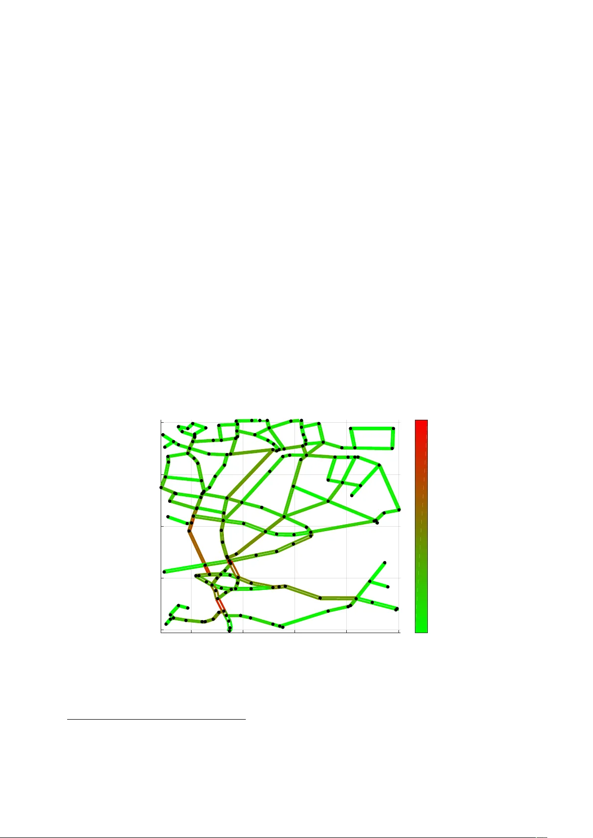
Dissertation ETH Zuric h No. 25597 Distributed con trol and game design: F rom strategic agen ts to programmable mac hines A dissertation submitted to attain the degree of Do ctor of Sciences of ETH Zuric h (Dr. sc. ETH Zuric h) presen ted b y Dario P accagnan Dott. Magistrale, Univ ersit` a degli studi di P ado v a, Italy M.Sc. T ec hnical Universit y of Denmark, Denmark b orn 19.01.1990 in T reviso citizen of Italy accepted on the recommendation of Prof. Dr. John Lygeros, examiner Prof. Dr. Andreas Krause, co-examiner Prof. Dr. Jason R. Marden, co-examiner 2018 ETH Zuric h IfA - Automatic Con trol Lab oratory ETL, Ph ysikstrasse 3 8092 Zuric h, Switzerland c  Dario P accagnan, 2018 All Righ ts Reserv ed ISBN 978-3-906916-47-7 DOI 10.3929/ethz-b-000314981 A l la mia famiglia F atti non foste a viver c ome bruti, ma p er se guir virtute e c anosc enza. – Dan te Alighieri Ac kno wledgemen ts First and foremost, I would lik e to express my gratitude to m y PhD Advisor, Prof. John Lygeros. While this thesis w ould not be in its current shap e without his guidance and supp ort, his contribution is far broader than that. Most of all, I w ould lik e to thank him for his unconditional trust, freedom and balance. On one hand, he allo w ed me to pursue any researc h direction I found exciting and relev an t, on the other he has alwa ys b een presen t to counsel me on a range of diﬀerent topics - technical and non. A sp ecial thanks go es for alw a ys b elieving in me and for helping me to set and pursue my goals. Lo oking bac k at when I mo v ed my ﬁrst steps at our institute, I can safely say that I ha v e gro wn not only on the technical side, but all around as a researcher. Let me keep it simple: thank you for everything! It w as an incredible luc k to work with Prof. Jason Marden who agreed to host me in San ta Barbara, without ever meeting with me b efore. I still remember when I walk ed in y our oﬃce for the ﬁrst time and I told you “I ha ve ten ideas to discuss with you”. Y ou listened to me extremely carefully for one hour. As a result, few days later we begun w orking on a completely diﬀerent topic. I am not sure whether y ou simply did not like an y of the ideas or maybe though t I should ha v e listened to yours ﬁrst. Nev ertheless, from that p oin t onw ards, it has b een an amazing journey and our collab oration has b een one of the most exciting I hav e ev er had. I would lik e to thank y ou for all the time you dedicated me, for y ou sharp-thinking, for your patience, and, amongst ev erything, for the en th usiasm you instilled in me: I hop e this is just the b eginning. Thanks to Prof. Andreas Krause for agreeing to serv e on my PhD committee and for meeting with me to discuss the con tent of this thesis, regardless of the tight schedule. I feel truly blessed and honored to hav e met and in teracted with Prof. Maria Elena V alc her. Not only has she giv en me con tinuous supp ort during the y ears, but she has sho wn me what it means to be an unparalleled advisor. Energy , passion, crystal-clear reasoning, unrestricted supp ort to her studen ts are only a few of her ev eryday’s ingredi- en ts. Most imp ortantly , I w ould like to thank her for b eing the ﬁrst p erson that b eliev ed in me, for in tro ducing me to control theory and for allo wing me to take oﬀ at DTU. Thank y ou for b eing a ligh thouse. I am deeply indebted with the new Professors of our institute Prof. Florian D¨ orﬂer and Prof. Mary am Kamgarpour. Thank you Florian for “taking me clim bing”, for all the adven tures in the mountains w e had together, for the advices y ou ga v e me when I w as only a newbie at IfA, and for putting me in con tact with Prof. Marden. Mary am, a i sincere thanks go es to y ou for y our supp ort and collab oration during the early stages of m y PhD. I remem b er vividly ho w m uc h help and en th usiasm y ou put in teac hing me ho w to write m y “ﬁrst article”. If all of this is p ossible, it is in go o d part also thanks to you. The atmosphere w e breath at IfA is absolutely incredible: a great mix of hard- w orking, p ositive energy , and friendship. Sometimes, b en t ov er our pap ers, w e seem to forget ho w lucky w e are. F ortunately (or not), as so on as w e step out of the ETH domain, we get reminded of what a privilege this is. I would like to express m y greatest gratitude to all those p eople that made this place what it is. In this regard, there are man y colleagues I should thank, but I limit myself to the essen tial. First of all, I w ould lik e to thank Basilio and F rancesca for sharing with me a go o d half of their PhDs, and coun tless hours on the b oard conjecturing results that would b e prov ed wrong only a few hours later. I wish b oth of you a brilliant career as y ou truly deserve. A v ery sp ecial thanks is due to Nicol` o for sharing inn umerable momen ts inside and outside of the oﬃce, for the many jokes w e hav e b een laughing of, and for the unmissable extra slice of cake (Lucia’s). A big thanks goes to the Italian Gang - Basilio, F rancesca, Nicol` o, Giampaolo, Marcello, Sav erio - for the countless adv en tures, and for making me feel as IfA was the extension of my time in high school. Thank y ou T ony for b eing suc h a p ositive, cheerful and selﬂess p erson. Thank you Peyman for the numerous research discussions we had: I feel there is a lot to learn form y ou. Thanks to the dream team - Juan, Marcello, P aul - for all the mountains adv en tures w e shared: I will hardly forget when w e set fo ot on the Dammazwillinge for the ﬁrst time. I am conﬁdent you will not forget either. A sp ecial thanks go es to Paul for b eing a terriﬁc oﬃce mate, and for sharing the ﬁrst years of your PhD with me, often out in the Alps. At this p oin t, I feel I o w e a big thanks to our secretaries, Sabrina and T anja, for making everything run incredibly smo oth and for b eing extremely helpful with really anything. “If there is a solution, we will ﬁnd it” Sabrina told me once, and this prett y muc h says it all. A t a p ersonal lev el, I w ould lik e to thank all m y friends in Zurich and elsewhere, in particular Chiara for the gazillions hours w e sp en t clim bing together, F ederica for b eing a terriﬁc housemate, Martina and Alessandro for hosting me after my return from the US. A line of his own is needed (and probably not enough) to thank Alessio: a v ery sp ecial thought go es to you for all the things w e wen t through together, wa y to o man y to recall. I will nev er forget the 20-hours day on the Allighesi ferrata, our ﬁrst clim bing route in the dolomites, or simply the usual giro di Ca’ T ron. Amongst ev erything, I w ould like to thank you for teaching me to b e ambitious, to ﬁght, to never giv e up and to endure pain. Last, I w an t to thank you for alwa ys ﬁnding time to meet with me (the usual run) when I come bac k from Zurich, regardless of our busy lives. A t this stage, it feels quite diﬃcult to ﬁnd the right words to thank those who con tributed the most to all of this. Thanks to the b ottom of m y heart to m y family and in particular to m y parents and brother. Mum and Dad, y ou hav e b een a guiding force throughout all these y ears. I w ould lik e to thank you for the curiosit y y ou instilled in ii me, for giving me a great education and making me understand its imp ortance. I am incredibly grateful for the unconditional supp ort I received, for the freedom you ga v e me in pursuing my o wn path, and for teaching me that great things happ en only if you dare trying. Y ou hav e set the bar quite high, and if I’ll ev er b e able to b e half as go o d as y ou ha v e b een, I’ll consider myself satisﬁed. A w arm thanks go es to my brother for sho wing me the w a y , for all the opp ortunities y ou gav e me, and for b eing an example of what one can ac hiev e with a “little” amoun t of constan t eﬀort. P erhaps I should thank y ou for those initial english lesson y ou ga ve me when I w as only a newbie, but I am conﬁden t the idea of sho wing me your b elo v ed “green english textb o ok” already made up for that. Finally , I ow e a huge, sincere and heartfelt thanks to Erisa. First and foremost for teac hing me (slowly but surely) the meaning of we , for your lo ve and patience, and for b earing with me “doing science”, probably the hardest amongst all. On the latter topic, I am indebted with y ou for reading through m y pap ers many times, for teaching me that “things need to get done” and, more in general, for b eing a great counsellor. Quite a few things ha ve changed since the ﬁrst time you “forced” me to buy the Zurich-Copenhagen tic k et, but I am very excited ab out all that come next, to gether . Dario P accagnan Zuric h, No vem b er 2018 iii iv Ringraziamen ti Innanzitutto, v orrei esprimere la mia gratitudine al mio PhD Advisor, il Prof. John Lygeros. Anche se questa tesi non sarebb e nella sua forma attuale senza la sua guida, il suo contributo non si limita certamen te a questo. V orrei ringraziarlo, in particolare, p er la ﬁducia datami, la lib ert` a e l’equilibrio. Da un lato, mi ha p ermesso di intraprendere qualsiasi direzione di ricerca trov assi interessan te, dall’altro ` e sempre stato presente p er consigliarmi su una serie di argomen ti diversi - tecnici e non. Devo un ringraziamen to sp eciale al Prof. Lygeros per a v er sempre creduto in me e per a v ermi aiutato a ﬁssare e raggiungere i miei obiettivi. Riv olgendo lo sguardo a quando ho mosso i primi passi nel nostro istituto, p osso dire di essere cresciuto non solo dal pun to di vista tecnico, ma anc he come ricercatore: grazie di tutto! E’ stata una fortuna incredibile lav orare con il Prof. Jason Marden, il quale ha accettato di ospitarmi a San ta Barbara senza a vermi incon trato prima. Ricordo b ene quando sono en trato nel tuo uﬃcio p er la prima v olta dicendo “Ho dieci idee che vorrei discutere con te”. Mi hai ascoltato con estrema attenzione p er pi ` u di un’ora. P o c hi giorni dopo, sta v amo la v orando su un argomen to completamente div erso. F orse non ti sono piaciute le mie idee, o probabilmen te avrei do vuto ascoltare prima le tue. T uttavia, da quel momen to in p oi, ` e cominciato un b ellissimo viaggio e la nostra collab orazione ` e stata una delle pi` u en tusiasman ti c he abbia mai a vuto. V orrei ringraziarti per tutto il temp o c he mi hai dedicato, per la tua pazienza e, sopratutto, p er l’en tusiasmo c he mi hai infuso: sp ero questo sia solo l’inizio. V orrei ringraziare il Prof. Andreas Krause p er av er accettato il ruolo di esaminatore esterno e p er a v ermi incontrato p er discutere il con tenuto di questa tesi. Sono da vv ero onorato di av er incontrato e in teragito con la Prof. Maria Elena V alcher. Non solo mi ha dato un sostegno con tin uo nel corso degli anni, ma mi ha anche mostrato cosa signiﬁca essere un Advisor senza pari. Energia, passione, ragionamento cristallino, sostegno ai suoi studenti, sono solo alcuni degli ingredien ti della sua vita quotidiana. V orrei ringraziarla, in particolare, p er essere la prima p ersona c he ha creduto in me, p er a v ermi introdotto alla teoria del controllo e p er av ermi spinto ad andare al DTU. Sono profondamen te in debito con i n uovi professori del nostro istituto, il Prof. Flo- rian D¨ orﬂer e la Prof. Maryam Kamgarp our. Grazie Florian p er ”p ortarmi a scalare”, p er tutte le a vv en ture in montagna che abbiamo avuto insieme, p er i consigli c he mi hai dato quando ero solo un novizio all’IfA, e p er av ermi messo in contatto con il Prof. Marden. Mary am, un sincero ringraziamento v a a te p er il tuo sostegno e la tua collab o- v razione duran te le prime fasi del mio dottorato. Ricordo molto b ene quan to en tusiasmo ed energia hai messo nell’insegnarmi a scrivere il mio “primo articolo”. Se tutto questo ` e p ossibile, ` e in buona parte anc he grazie a te. L’atmosfera c he respiriamo all’IfA ` e assolutamente incredibile: un p erfetto mix di la v oro, energia p ositiv a e amicizia. A volte, piegati sui nostri articoli, ﬁniamo p er di- men ticarci di quanto siamo co ccolati. F ortunatamente (o forse no), non app ena usciamo dal nostro uﬃcio, ci accorgiamo immediatamen te di c he privilegio sia questo. V orrei esprimere la mia pi ` u grande gratitudine a tutte le p ersone che hanno reso questo luogo quello c he ` e. A questo proposito, mentre dovrei ringraziare molti colleghi, mi limiter` o solamen te all’essenziale. Prima di tutto, vorrei ringraziare Basilio e F rancesca p er a v er condiviso con me una buona met` a dei loro dottorati, e inn umerev oli ore alla la v agna a congetturare risultati che si sarebb ero riv elati errati solo p o c he ore dop o. Auguro ad en- tram bi una brillante carriera. Un ringraziamento sp eciale v a a Nicol` o p er av er condiviso moltissimi momenti dentro e fuori dall’uﬃcio, p er le tan te battute di cui abbiamo riso e per l’immancabile fetta di torta in pi` u (confezionata da Lucia). Un sen tito ringrazi- amen to v a all’Italian Gang - Basilio, F rancesca, Nicol` o, Giampaolo, Marcello, Sav erio - p er le innumerev oli avv enture, e p er a vermi fatto sen tire come se IfA fosse la contin u- azione del liceo. Grazie T on y p er essere una persona cos ` ı p ositiv a, allegra ed altruista. Grazie Peyman p er le n umerose discussioni che abbiamo avuto: ho l’impressione che ci sia molto da imparare da te. Grazie al Dream T eam - Juan, Marcello, P aul - p er tutte le a vv en ture in mon tagna che abbiamo vissuto insieme: non dimen tic her` o mai quando mettemmo piede sul Dammazwillinge p er la prima volta. Sono con vinto non lo dimen- tic herete neanc he voi. Un ringraziamen to sp eciale v a a P aul per essere stato un fan tastico compagno di uﬃcio e p er av er condiviso con me, sp esso sulle Alpi, i primi anni in IfA. A questo pun to, ` e d’obbligo un ringraziamento alle nostre segretarie, Sabrina e T anja, p er a v er fatto funzionare tutto in maniera imp eccabile: “se c’ ` e una soluzione, la trov eremo” ha detto Sabrina pi ` u di una volta. A liv ello p ersonale, v orrei ringraziare tutti i miei amici di Zurigo e non solo, in particolare Chiara p er le inn umerev oli ore passate assieme arrampicando, F ederica per essere stata una fantastica compagna di casa, Martina e Alessandro p er av ermi ospitato dop o il ritorno dagli Stati Uniti. Devo un p ensiero molto sp eciale (e com unque non suﬃcien te) ad Alessio per tutte le cose c he abbiamo vissuto insieme, troppe per ricordarle tutte. Non dimentic her` o mai la giornata di 20 ore sulla ferrata Allighesi, la nostra prima via d’arrampicata nelle Dolomiti, o semplicemente il solito giro di Ca’ T ron. V orrei ringraziarti sopratutto p er av ermi insegnato ad essere ambizioso, a com battere, a non arrendermi mai e a sopp ortare la fatica. Inﬁne, ti dev o ringraziare p er a ver sempre trov ato il temp o di incontrarmi al mio ritorno da Zurigo (la solita corsa), indipendentemen te dagli inn umerev oli imp egni. Giun to a questo punto, risulta diﬃcile trov are le parole giuste p er ringraziare coloro c he hanno contribuito maggiormente a tutto questo. Grazie di cuore alla mia famiglia, vi in particolare ai miei genitori ed a mio fratello. Mamma e pap` a, siete stati una forza trainan te in tutti questi anni. V orrei ringraziarvi p er la curiosit` a c he mi av ete instillato, p er a vermi dato un’educazione in vidiabile e per av ermene fatto capire l’imp ortanza. Sono incredibilmen te grato p er il sostegno incondizionato che mi av ete dato in tutti questi anni, p er la libert` a c he ho ricevuto nel seguire la mia strada, e p er a vermi insegnato c he le cose pi ` u b elle accadono solo a c hi ha il coraggio di prov are. Avete p osto l’asticella molto in alto, e se mai riuscir` o a raggiungerne la met` a, mi considerer` o so ddisfatto. Un caloroso ringraziamen to v a a Diego p er a v ermi indicato la strada, p er tutte le opp ortunit` a che mi hai oﬀerto, e p er essere un esempio di ci` o c he si pu` o ottenere con un “piccolo” sforzo quotidiano. F orse dovrei ringraziarti p er quelle prime lezioni di inglese che mi hai dato quando ero solo un principiante, ma sono sicuro che il piacere di mostrarmi il tuo amato “libro v erde” ti ha gi` a ripagato. Inﬁne, dev o un enorme, sincero e sentito grazie ad Erisa. Innanzitutto p er av ermi insegnato il signiﬁcato della parola noi , per il tuo amore e pazienza, e p er sopp ortarmi quando sono “imp egnato con la scienza”, probabilmente la pi ` u diﬃcile tra tutte le pro v e. Ti devo un ringraziamen to sp eciale p er a v er riletto pi ` u e pi ` u volte i miei articoli, p er a v ermi insegnato c he “` e inutile p erdere temp o a cincischiare, bisogna ﬁnire il lav oro” e, pi ` u in generale, p er essere un grande consigliere. Molte cose sono cambiate dalla prima v olta che mi hai “costretto” a comprare il biglietto Zurigo-Cop enhagen, e sono elettriz- zato p er tutto ci` o che ci asp etta, insieme . Dario P accagnan Zurigo, No v embre 2018 vii viii Abstract Large scale systems are forecasted to greatly impact our future liv es thanks to their wide ranging applications including co operative rob otics, mobilit y on demand, resource and task allo cation, supply chain managemen t, and many more. While technological dev elopmen ts ha v e pa v ed the wa y for the realization of suc h futuristic systems, we ha v e a limited grasp on ho w to co ordinate the b ehavior of their individual comp onen ts to ac hiev e the desired global ob jectiv e. With the ob jective of adv ancing our understanding, this thesis fo cus on the analysis and co ordination of large scale systems without the need of a cen tralized authority . A t a high lev el, we distinguish these systems dep ending on wether they are comp osed of c o op er ative or non-c o op er ative subsystems. In regard to the ﬁrst class, a k ey challenge is the design of lo cal decision rules for the individual comp onents to guarantee that the collective b ehavior is desirable with respect to a global ob jective. Non-co op erativ e systems, on the other hand, require a more careful thinking in that the designer needs to tak e in to accoun t the self-interested nature of the agents. In b oth cases, the need for distributed proto cols stems from the observ ation that cen tralized decision making is prohibited due to the scale and priv acy requirement asso ciated with typical systems. In the ﬁrst part of this thesis, we fo cus on the co ordination of a large num b er of non- c o op er ative agents. More sp eciﬁcally , w e consider strategic decision making problems where each agent’s ob jectiv e is a function of the aggregate behavior of the p opulation. Examples are ubiquitous and include so cial and traﬃc net works, demand-resp onse mar- k ets, v accination campaigns, to name just a few. W e presen t tw o cohesive con tributions. First, we compare the p erformance of an equilibrium allo cation with that of an opti- mal allo cation, that is an allo cation where a common w elfare function is maximized. W e prop ose conditions under whic h all Nash equilibrium allo cations are eﬃcien t, i.e., are de- sirable from a macroscopic standp oin t. In the journey to w ards this goal, w e pro v e a no v el result b ounding the distance b et w een the strategies at a Nash and at a W ardrop equi- librium that might b e of indep enden t in terest. Second, w e sho w how to deriv e scalable algorithms that guide agents to wards an equilibrium allo cation, i.e., a stable conﬁgura- tion where no agent has any incen tive to deviate. When the corresp onding equilibria are eﬃcient, these algorithms attain the global ob jectiv e and resp ect the agen ts’ selﬁsh nature. In the second part of this thesis, we fo cus on the co ordination of c o op er ative agen ts. W e consider large-scale resource allo cation problems, where a n umber of agents need to b e ix allo cated to a set of resources, with the goal of join tly maximizing a giv en submodular or sup ermo dular set function. Applications include sensor allo cation problems, distributed cac hing, data summarization, and man y more. Since this class of problems is computa- tionally intractable, we aim at deriving tractable algorithms for attaining appro ximate solutions, ideally with the b est p ossible appro ximation ratio. W e approach the problem from a game-theoretic p ersp ectiv e and ask the follo wing question: ho w should we design agen ts’ utilities so that an y equilibrium conﬁguration recov ers a large fraction of the opti- m um welfare? In order to answ er this question, w e introduce a no vel framew ork providing a tight expression for the worst-case p erformance (price of anarc hy) as a function of the c hosen utilities. Lev eraging this result, we show ho w to design utilit y functions so as to optimize the price of anarc hy b y means of a tractable linear program. The upshot of our con tribution is the design of algorithms that are distributed, eﬃcien t, and whose p erfor- mance is certiﬁed to be on par or better than that of existing (and centralized) schemes. x Sommario I sistemi tecnologici su larga scala promettono di migliorare sensibilmen te la qualit` a della nostra vita futura grazie alle loro n umerose applicazioni, tra cui la rob otica co op erativ a, la mobilit` a su ric hiesta, l’allo cazione di risorse, la gestione della supply chain. Nonos- tan te gli sviluppi tecnologici abbiano ap erto la strada alla realizzazione di questi sistemi futuristici, abbiamo una conoscenza limitata su come co ordinare i singoli comp onenti p er ottenere l’obiettiv o macroscopico desiderato. Questa tesi si concen tra sull’analisi e il co ordinamen to di sistemi su larga scala privi di un’autorit` a centralizzata, con l’obiettivo di migliorarne la comprensione ed il funzion- amen to. Ad alto liv ello, distinguiamo questi sistemi a seconda che essi siano co op erativi o meno. Una sﬁda chia v e in relazione ai sistemi co operativi ` e la progettazione di al- goritmi di con trollo p er le singole comp onen ti c he garantiscano il raggiungimento di un predeterminato obiettiv o globale. I sistemi non co op erativi, d’altra parte, richiedono una maggiore attenzione in quanto ` e necessario tenere in considerazione la natura egoistica degli agenti. In entram bi i casi, l’utilizzo di proto colli distribuiti ` e reso necessario dalle dimensioni di tali sistemi e dai requisiti di priv acy che vi sono asso ciati. Nella prima parte di questa tesi, ci concentriamo sul coordinamento di sistemi non co op erativi. Pi` u sp eciﬁcamen te, consideriamo problemi strategici in cui l’obiettiv o di ciascun agente ` e inﬂuenzato del comportamento aggregato della p op olazione. Esempi di tali sistemi comprendono i so cial netw orks, le reti stradali, i mercati azionari. Nel seguito presen tiamo due risultati co esivi. In primo luogo, confron tiamo la p erformance di un’allo cazione di equilibrio con la p erformance di un’allo cazione ottimale, cio ` e di un’allo cazione in cui viene massimizzata una funzione obiettiv o comune. Prop oniamo p oi condizioni c he garantiscono l’eﬃcienza di tutte le allo cazioni di equilibrio. Nel p ercorso v erso questo obiettivo, otteniamo un risultato c he delimita la distanza tra gli equilibri di Nash e W ardrop e che potrebb e essere di in teresse indip endente. In secondo luogo, progettiamo algoritmi scalabili c he guidano gli agen ti verso un’allo cazione di equilibrio, cio ` e una conﬁgurazione stabile in cui nessun agen te ha alcun incen tiv o a deviare. Quando tali equilibri sono eﬃcienti, questi algoritmi raggiungono l’obiettivo globale e risp ettano la natura individualistica degli agen ti. Nella seconda parte di questa tesi, ci concen triamo sul con trollo di sistemi co oper- ativi. In particolare, consideriamo problemi di allo cazione delle risorse su larga scala, do v e un insieme di risorse dev e essere assegnato ad un ﬁssato n umero di agen ti, con l’obiettiv o di massimizzare una funzione obiettivo globale, submo dulare o sup ermo du- xi lare. Le applicazioni includono problemi di allo cazione dei sensori, cac hing distribuito, data summarization e molto altro ancora. P oic h´ e questa classe di problemi ` e in tratta- bile dal pun to di vista computazionale, ci preﬁggiamo di ricav are soluzioni approssimate con algoritmi eﬃcien ti, idealmente con il miglior rapp orto di approssimazione p ossibile. F orm uliamo questo problema con il linguaggio della teoria dei gio chi e ci poniamo la seguen te domanda: come progettare le funzioni obiettiv o da assegnare agli agen ti in mo do c he ogni conﬁgurazione di equilibrio pro duca la massima frazione del v alore ot- timo? P er risp ondere a questa domanda, in tro duciamo un n uo v o meto do per calcolare in maniera esatta la qualit` a di un equilibrio in relazione alle funzioni obiettivo scelte (price of anarch y). Sfruttando questo risultato, mostriamo come costruire tali funzioni obiet- tiv o in mo do da massimizzare la p erformance dei corrisp ondenti equilibri grazie ad un programma lineare ausiliario. Il risultato ﬁnale ` e la progettazione di algoritmi distribuiti ed eﬃcien ti, il cui rapp orto di approssimazione ` e alla pari o sup eriore a quello di molti sc hemi (cen tralizzati) comunemen te usati. xii Con ten ts Ac kno wledgemen ts i Ringraziamen ti v Abstract ix Sommario xi Notation xvii 1 Ov erview 1 1.1 Outline and con tributions . . . . . . . . . . . . . . . . . . . . . . . . . . 2 1.1.1 P art I: strategic agents . . . . . . . . . . . . . . . . . . . . . . . . 2 1.1.2 P art I I: programmable mac hines . . . . . . . . . . . . . . . . . . . 3 1.2 Publications . . . . . . . . . . . . . . . . . . . . . . . . . . . . . . . . . . 5 1.2.1 P art I: strategic agents . . . . . . . . . . . . . . . . . . . . . . . . 5 1.2.2 P art I I: programmable mac hines . . . . . . . . . . . . . . . . . . . 6 1.2.3 Other publications . . . . . . . . . . . . . . . . . . . . . . . . . . 6 I Strategic agen ts: aggregativ e games 9 2 In tro duction 11 2.1 Equilibrium eﬃciency and algorithms . . . . . . . . . . . . . . . . . . . . 13 2.2 Related w orks . . . . . . . . . . . . . . . . . . . . . . . . . . . . . . . . . 14 3 Mathematical preliminaries 17 3.1 Op erator prop erties . . . . . . . . . . . . . . . . . . . . . . . . . . . . . . 17 3.2 V ariational inequalities . . . . . . . . . . . . . . . . . . . . . . . . . . . . 18 4 Nash and W ardrop equilibria in aggregativ e games 23 xiii 4.1 Equilibria with coupling constrain ts . . . . . . . . . . . . . . . . . . . . . 23 4.2 V ariational reform ulations . . . . . . . . . . . . . . . . . . . . . . . . . . 25 4.3 Suﬃcien t conditions for monotonicit y . . . . . . . . . . . . . . . . . . . . 28 4.3.1 Linear price function . . . . . . . . . . . . . . . . . . . . . . . . . 29 4.3.2 Diagonal price function . . . . . . . . . . . . . . . . . . . . . . . . 30 4.4 App endix . . . . . . . . . . . . . . . . . . . . . . . . . . . . . . . . . . . 32 4.4.1 Pro ofs of the results presen ted in Sections 4.2 and 4.3 . . . . . . . 32 5 Equilibria and eﬃciency in large p opulations 37 5.1 Distance b et w een Nash and W ardrop equilibria . . . . . . . . . . . . . . 37 5.2 Equilibrium eﬃciency: the price of anarch y . . . . . . . . . . . . . . . . . 40 5.2.1 Linear price function . . . . . . . . . . . . . . . . . . . . . . . . . 41 5.2.2 Diagonal price function . . . . . . . . . . . . . . . . . . . . . . . . 42 5.3 App endix . . . . . . . . . . . . . . . . . . . . . . . . . . . . . . . . . . . 45 5.3.1 Pro ofs of the results presen ted in Section 5.1 . . . . . . . . . . . . 45 5.3.2 Pro ofs of the results presen ted in Section 5.2 . . . . . . . . . . . . 47 6 Decen tralized algorithms 53 6.1 Best-resp onse algorithm for W ardrop equilibrium . . . . . . . . . . . . . 55 6.2 Gradien t-based algorithm for Nash and W ardrop equilibria . . . . . . . . 57 6.3 App endix . . . . . . . . . . . . . . . . . . . . . . . . . . . . . . . . . . . 59 6.3.1 Pro ofs of the results presen ted in Sections 6.1 and 6.2 . . . . . . . 59 7 Applications 63 7.1 Charging of electric v ehicles . . . . . . . . . . . . . . . . . . . . . . . . . 63 7.1.1 Theoretical guaran tees . . . . . . . . . . . . . . . . . . . . . . . . 64 7.1.2 Numerical analysis . . . . . . . . . . . . . . . . . . . . . . . . . . 66 7.2 Route c hoice in a road netw ork . . . . . . . . . . . . . . . . . . . . . . . 70 7.2.1 Theoretical guaran tees . . . . . . . . . . . . . . . . . . . . . . . . 73 7.2.2 Numerical analysis . . . . . . . . . . . . . . . . . . . . . . . . . . 74 7.3 App endix . . . . . . . . . . . . . . . . . . . . . . . . . . . . . . . . . . . 76 7.3.1 Pro ofs of the results presen ted in Sections 7.1 and 7.2 . . . . . . . 76 xiv I I Programmable mac hines: game design 79 8 In tro duction 81 8.1 The game-design framew ork . . . . . . . . . . . . . . . . . . . . . . . . . 81 8.2 The general m ultiagen t maximum cov erage . . . . . . . . . . . . . . . . . 83 8.2.1 Applications . . . . . . . . . . . . . . . . . . . . . . . . . . . . . . 84 8.3 Related w ork . . . . . . . . . . . . . . . . . . . . . . . . . . . . . . . . . 85 9 Mathematical preliminaries 89 9.1 Strategic-form games and equilibrium concepts . . . . . . . . . . . . . . . 89 9.2 P oten tial games and congestion games . . . . . . . . . . . . . . . . . . . 91 9.3 Price of anarc h y and smo othness . . . . . . . . . . . . . . . . . . . . . . 94 9.3.1 The question of tigh tness . . . . . . . . . . . . . . . . . . . . . . . 96 9.4 Complexit y of computing equilibria . . . . . . . . . . . . . . . . . . . . . 97 10 Tight price of anarch y and utilit y design: a linear program approac h 101 10.1 The price of anarch y as p erformance metric . . . . . . . . . . . . . . . . 101 10.2 The limitations of the smo othness framework . . . . . . . . . . . . . . . . 105 10.3 A tight price of anarch y . . . . . . . . . . . . . . . . . . . . . . . . . . . 107 10.3.1 Primal form ulation . . . . . . . . . . . . . . . . . . . . . . . . . . 109 10.3.2 Dual form ulation . . . . . . . . . . . . . . . . . . . . . . . . . . . 111 10.3.3 Related w orks . . . . . . . . . . . . . . . . . . . . . . . . . . . . . 113 10.4 Optimal utility design via linear programming . . . . . . . . . . . . . . . 114 10.5 App endix . . . . . . . . . . . . . . . . . . . . . . . . . . . . . . . . . . . 115 10.5.1 Pro ofs of the results presen ted in Section 10.2 . . . . . . . . . . . 115 10.5.2 Pro ofs of the results presen ted in Section 10.3 . . . . . . . . . . . 116 10.5.3 Pro ofs of the results presen ted in Section 10.4 . . . . . . . . . . . 127 11 Submo dular, sup ermo dular, co vering problems 131 11.1 The case of submo dular welfare function . . . . . . . . . . . . . . . . . . 132 11.1.1 Impro v ed approximation and comparison with existing result . . . 136 11.2 Cov ering problems . . . . . . . . . . . . . . . . . . . . . . . . . . . . . . 137 11.3 The case of sup ermo dular w elfare function . . . . . . . . . . . . . . . . . 139 11.4 App endix . . . . . . . . . . . . . . . . . . . . . . . . . . . . . . . . . . . 141 11.4.1 Pro ofs of the results presen ted in Section 11.1 . . . . . . . . . . . 141 xv 11.4.2 Pro ofs of the results presen ted in Section 11.2 . . . . . . . . . . . 145 11.4.3 Pro ofs of the results presen ted in Section 11.3 . . . . . . . . . . . 147 12 Applications 149 12.1 The vehicle target allo cation problem . . . . . . . . . . . . . . . . . . . . 149 12.2 Distributed caching . . . . . . . . . . . . . . . . . . . . . . . . . . . . . . 152 I I I Conclusion 157 13 Conclusions and outlook 159 13.1 Part I: strategic agents . . . . . . . . . . . . . . . . . . . . . . . . . . . . 159 13.1.1 F urther researc h directions . . . . . . . . . . . . . . . . . . . . . . 159 13.2 Part I I: programmable machines . . . . . . . . . . . . . . . . . . . . . . . 161 13.2.1 F urther researc h directions . . . . . . . . . . . . . . . . . . . . . . 162 Bibliograph y 165 xvi Notation Acron yms A CCE opt a v erage coarse correlated equilibrium BR b est-resp onse dynamics CCE coarse correlated equilibrium GMMC general m ultiagen t weigh ted maximum co v erage KKT Karush-Kuhn-T uc ker LP linear program MMC m ultiagen t weigh ted maximum co v erage MNE mixed Nash equilibrium NE Nash equilibrium P oA price of anarc h y Sym b ols : = equal b y deﬁnition N , N 0 set of natural n um b ers, set of natural num b ers including zero R , R > 0 , R ≥ 0 set of real, p ositiv e real, non negativ e real num b ers [ p ], [ p ] 0 set of in tegers { 1 , . . . , p } , set of in tegers v { 0 , 1 , . . . , p } [ a, b ] in terv al of real num bers x ∈ R with a ≤ x ≤ b 1 n , 0 n , e i ∈ R n v ector of unit en tries, vector of zero entries, i th canonical v ector I n iden tit y matrix I n ∈ R n × n A  0 (  0) p ositive deﬁnite (semi-) A ∈ R n × n , i.e., x > Ax > 0 ( ≥ 0) , ∀ x 6 = 0 k x k 2-norm of x ∈ R n k A k induced 2-norm of A ∈ R n × n , k A k := sup x 6 =0 k Ax k k x k λ min ( A ), λ max ( A ) minim um, maxim um eigenv alue of the symmetric matrix A ∈ R n × n [ A ] ij = A ij , elemen t in p osition ( i, j ) of the matrix A A ⊗ B Kronec k er pro duct of the matrices A, B [ x i ] m i =1 stac k ed vector [ x i ] m i =1 : = [( x 1 ) > , . . . , ( x m ) > ] > = [ x 1 ; . . . ; x m ] , x i ∈ R n × 1 xvii Π X ( y ) metric pro jection of y ∈ R n on to X ⊆ R n , see Deﬁnition 5 f ( x ) = O ( g ( x )) big O notation: lim x →∞ f ( x ) g ( x ) = 0 f 0 ( x ) deriv ative of diﬀerentiable f : R → R ∇ x f ( x ) ∈ R n × m Jacobian of diﬀeren tiable f : R n → R m , i.e., [ ∇ x f ( x )] ij : = ∂ g j ( x ) ∂ x i P n i =1 X i Mink o wski sum of the sets {X i } n i =1 VI( X , F ) v ariational inequality with set X and op erator F , see Deﬁnition 4 U [ a, b ] uniform distribution on the real in terv al [ a, b ] 1 { f ( x ) ≥ 0 } indicator function of the set { x ∈ R n s.t. f ( x ) ≥ 0 } , f : R n → R | S | cardinalit y of the (ﬁnite) set S Reserv ed sym b ols P art I M num b er of play ers n dimension of pla y ers’ strategy vectors x i ∈ R n strategy v ector of pla yer i ∈ [ M ] x − i ∈ R n ( M − 1) strategy v ector of all play ers but i ∈ [ M ] X i ⊆ R n lo cal constrain t set of pla yer i ∈ [ M ] X pro duct of lo cal constraint sets X : = X 1 × · · · × X M C ⊆ R M n coupling constrain t set σ ( x ) ∈ R n a v erage of strategies σ ( x ) : = 1 M P M i =1 x i J i ( x i , σ ( x )) cost function of pla yer i ∈ [ M ], J i : R n × R n → R G aggregativ e game deﬁned in ( 4.3 ) x N , x W Nash, W ardrop equilibrium according to Deﬁnitions 6 and 7 J S ( σ ( x )) so cial cost function, J S : R n → R , see Deﬁnition 8 P art I I e Euler’s num b er R set of resources R = { r 1 , . . . , r m } v r v alue of resource r ∈ R , v r ∈ R ≥ 0 n n umber of agents a i strategy of pla y er i ∈ [ n ] A i strategy set of pla y er i ∈ [ n ] A pro duct of agen ts’ strategy sets A : = A 1 × · · · × A n W ( a ) w elfare function W : 2 R × · · · × 2 R → R ≥ 0 | a | r n um b er of agen ts selecting resource r in allo cation a w ( j ) w elfare basis function w : [ n ] → R ≥ 0 u i ( a ) utilit y function of agent i ∈ [ n ], u i : A → R f ( j ) distribution rule f : [ n ] → R ≥ 0 a ne pure Nash equilibrium strategy according to Deﬁnition 10 f G , f SV , f MC distribution rules in tro duced in ( 10.5 ) and Deﬁnition 24 xviii Complexit y classes P deterministic p olynomial time class N P nondeterministic p olynomial time class P LS p olynomial lo cal search class P P AD p olynomial parit y argumen ts on directed graphs class xix xx CHAPTER 1 Ov erview Large scale systems ha v e enormous p oten tial for solving man y of the curren t so cietal c hallenges. Rob otic net works can op erate in p ost-disaster en vironments and reduce the impact of nuclear, industrial or natural calamities [ Kun+12 ; Kit+99 ]. Fleets of autonomous cars are forecasted to revolutionize the future mobilit y and to reduce traﬃc congestion as w ell as p ollutan t emissions [ Spi+14 ]. Demand-resp onse schemes ha ve the p oten tial to allow for the integration of a large share of renew able resources [ Mot+16 ]. On a smaller scale, sw arms of “microb ots” promise groundbreaking results in medicine b y means of lo cal drug deliv ery [ Ser+15 ] or microsurgery [ ISA02 ]. While all the ab ov e-men tioned systems (and many more) can b e though t of as a col- lection of m ultiple subsystems or agents , we distinguish them in t w o categories dep ending on wether the corresponding subsystems ar e or ar e not co op erativ e. An example of coop- erativ e system is that of a drones sw arm p erforming a rescue mission. On the other hand, priv ately-owned self driving cars are non-co op erativ e, since eac h car’s ob jective is that of reac hing its destination as swiftly as p ossible, while resp ecting the traﬃc rules. Another example of non-co op erativ e large scale system is the electricit y reserv e mark et, where gen- erators sell their abilit y to increase or decrease their electricit y pro duction to the system op erator, whose ultimate ob jective is that of balancing pro duction and consumption. Figure 1.1 One of the main chal lenges in the op eration of b oth t yp es of systems is the design of lo c al de cision rules for the individual subsystems to guarantee that the col- lectiv e b ehavior is desirable with resp ect to a glob al obje ctive [ LM13 ]. With this resp ect, non-co op erativ e systems pose an additional la y er of diﬃcult y , in that preexisting lo cal ob jectiv es migh t not b e aligned with the system-lev el goal. As a concrete example consider on-demand ridesharing platforms suc h as Ub er, Lyft or Didi, where agen ts are represen ted b y h uman driv ers ho v ering around diﬀeren t city neighbors ( Figure 1.1 ). While drivers’ might p osition themselves in neigh b ors 1 that maximize their o wn proﬁt, the system-op erator migh t hav e a diﬀerent goal, e.g., to guaran tee a minim um cov erage of the cit y . F or this class of systems, it is not suﬃ- cien t to design lo cal decision rules to b e executed from each subsystem, but it is equally imp ortan t to inc entivize their adoption. The spatial distribution, priv acy requirements, scale, and quantit y of information asso ciated with t ypical systems do not allow for centralized comm unication and decision making, but require instead the use of distribute d pr oto c ols . In addition to the ab o v e requiremen ts, designing suc h proto cols is non-trivial due to the presence of heterogenous decision makers and informational constraints. T o complete the o verview, w e note that the quality of a control architecture is usually gauged b y several metrics including the satisfaction of the global ob jectiv e, the robustness to external disturbances, as w ell as the amoun t of information propagated through the communication netw ork. The goal of this thesis is to address the c hallenges previously discussed, with particular atten tion to the design of lo cal decision rules in relation to their corresp onding system- lev el p erformance. While in the ﬁrst part of the thesis w e fo cus on large scale non- c o op er ative system, we exploit some of the insigh t obtained therein to address, in the second part of the thesis, large scale c o op er ative system and prop ose no v el eﬃcien t distributed algorithms. 1.1 Outline and con tributions 1.1.1 P art I: strategic agen ts In the ﬁrst part of the thesis w e focus on large scale systems composed of str ate gic agents. Sp eciﬁcally , w e consider the framew ork of aver age aggr e gative games , where each agen t aims at minimizing a cost function that dep ends b oth on his decision and on the a verage p opulation strategy . Our ob jectiv e is t wofold. First, w e wish to understand to what exten t selﬁsh decision making reduces the system p erformance. W e do this using the notion of price of anarch y . Second, w e aim at the design of scalable and decen tralized algorithms that pro v ably conv erge to a Nash or a W ardrop equilibrium. W e ac hieve this lev eraging the theory of v ariational inequalities. Outline. Chapter 2 pro vides an informal introduction to the framew ork of aggregative games and describes how such games can b e used to model applications p ertaining to v arious ﬁelds. At the end of the chapter we review the existing literature and connect our w ork with it. In Chapter 3 we review the mathematical to ols needed throughout Part I of this thesis. In Chapter 4 w e formalize the notions of Nash and W ardrop equilibria in the presence of coupling constrain ts, and use the language of v ariational inequali- ties to reform ulate these problems. W e conclude the c hapter studying the monotonicity 2 prop erties of the v ariational inequality op erator asso ciated with the corresp onding equi- librium problems. In the ﬁrst part of Chapter 5 we study the relation b et ween Nash and W ardrop equilibria with particular atten tion to the distance b etw een the corresp onding strategies. In the second part of this chapter, w e leverage these results to b ound the p erformance degradation incurred when mo ving from a centralized solution to strategic decision making. In Chapter 6 w e present a b est-resp onse algorithm and a gradient- based algorithm that prov ably conv erge to a Nash or W ardrop equilibrium. W e conclude P art I with Chapter 7 , where w e demonstrate the results previously obtained to tw o large scale applications. Con tributions. The main con tributions of Part I of this thesis are con tained in Chap- ters 4 , 5 , 6 and 7 , and are detailed in the follo wing. (a) In Chapter 4 w e in tro duce the notion of W ardrop equilibrium as a condition on the agen ts’ strategies, rather than a condition on the aggregate b eha viour. This allo ws to address a larger class of equilibrium problems, compared to the existing literature. W e then study the relation b et w een Nash and W ardrop equilibrium strategies and show that, in a game with M play ers, their euclidean distance is upp er b ounded by O (1 / √ M ) when one of the corresp onding v ariational inequality is strongly monotone ( Theorem 1 ). This allows us to pro vide guaran tees on the ef- ﬁciency of Nash equilibria b y studying the eﬃciency of the corresp onding W ardrop equilibria ( Theorems 2 , 3 and 4 ). (b) In Chapter 6 we presen t a b est-resp onse and a gradien t-based algorithm that allow to compute a Nash or a W ardrop equilibrium in the presence of coupling constrain ts ( Theorems 5 and 6 ). (c) In Chapter 7 we apply the theoretical results previously deriv ed to i) co ordinate the charging proﬁle of a p opulation of electric v ehicles, and ii) to predict the trav el time distribution for a road traﬃc netw ork. The results w e obtain b oth in terms of equilibrium eﬃciency and algorithmic con vergence are nov el. 1.1.2 P art I I: programmable machines In the second part of the thesis w e fo cus on the con trol of large scale systems comp osed of multiple c o op er ative subsystems. W e assume that each subsystem (agent) is endo wed with computation and comm unication capabilities, and w e aim at achieving a global ob jectiv e through lo cal co ordination of the agents. More sp eciﬁcally , w e consider a class of combinatorial allocation problems, where eac h agent selects a subset of resources with the goal of join tly maximizing a given welfare function, additiv e ov er the resources. Since this class of problems is intractable, w e seek distributed algorithms that run in p olynomial time and give pro v able appro ximation guarantees. Rather than directly 3 sp ecifying a decision making pro cess, w e adopt the game design approac h, and assign to eac h agent a lo cal utility function. The fundamen tal question we seek to answ er in this part of the thesis is ho w to design local utilit y functions so that their selﬁsh maximization reco v ers a large fraction of the optimal welfare. Outline. In Chapter 8 we introduce the problem considered, discuss p otential applica- tions as w ell as related w orks. In Chapter 9 w e review the mathematical to ols needed for the developmen t of our work. In Chapter 10 we formulate the utilit y design question and tackle it in t w o steps. First, w e pro vide p erformance certiﬁcates for a giv en set of utilit y functions; second, we show ho w to design utilities that maximize the corre- sp onding worst-case p erformance. In Chapter 11 we sp ecialize the results to a class of submo dular, sup ermo dular and maximum cov erage problems. Finally , in Chapter 12 we presen t tw o applications: the vehicle-target assignmen t problem and a cov erage problem arising in distributed cac hing for mobile netw orks. Con tributions. The main contributions of Part I I of this thesis are contained in Chap- ters 10 , 11 and 12 and are detailed in the follo wing. (a) In Chapter 10 w e p ose the utilit y design problem and adopt the notion of price of anarc h y as the worst-case p erformance metric. W e show that traditional ap- proac hes used to quantify such performance metric are rather conserv ativ e and are not suited for the design problem considered here ( Theorem 7 ). Motiv ated by this shortcoming, w e propose a nov el framew ork to c ompute ( Theorems 8 and 9 ) and optimize ( Theorem 10 ) the price of anarch y as a function of the giv en utilities. In particular, we sho w that the utilit y design problem can be reform ulated as a tractable linear program. The upshot of this contributions is the p ossibilit y to apply the game design pro cedure to a broad class of problems. T o the b est of our kno wledge, this is the ﬁrst approach that allows to systematically compute and optimize the price of anarc hy . (b) In Chapter 11 we sp ecialize the previous results to the case of submo dular, maxi- m um cov erage, and sup ermo dular problems. Relative to the submo dular case, we obtain a no v el and fully explicit expression for the price of anarch y ( Theorem 11 ). W e further apply this result to determine the exact price of anarch y for the Shapley v alue and marginal contribution design metho dologies ( Corollary 4 ). These results are compared with previous (non tigh t and fragmen ted) results from the litera- ture, and are placed in the larger context of submo dular maximization sub ject to matroid constraints. Relative to the class of problems considered, we sho w how optimally-designed utilities pro vide an appro ximation ratio sup erior to the b est kno wn ratio 1 − c/e of [ SVW17 ]. 1 Relativ e to the case of multiagen t maxim um 1 The result of [ SVW17 ] improv es on the (1 − e − c ) /c of [ CC84 ], where c is the (total) curv ature of the welfare function [ CC84 ] and e the Euler’s num ber. 4 co v erage problems, w e obtain a nov el analytical expression for the price of anar- c h y ( Theorem 12 ), and subsume previous results in [ Gai09 ; RPM17 ]. Optimally designed utilities achiev e a 1 − 1 /e appro ximation, the best p ossible [ F ei98 ]. W e conclude the c hapter providing a tigh t expression for the price of anarch y in the case of sup ermo dular welfare function ( Theorem 13 ), and sho w that our result comple- men ts [ JM18 ; PM17b ]. Limitedly to this case, we observ e that optimally-designed utilit y functions pro vide a rather p o or appro ximation ratio. (c) In Chapter 12 w e test the p erformance of the prop osed algorithms on a task- allo cation problem, and on a cov erage problem arising in distributed mobile net- w orks. W e pro vide thorough sim ulation results and sho w the theoretical and nu- merical adv antages of our approach. 1.2 Publications This thesis contains a subset of the results deriv ed during the author’s studies as PhD studen t at ETH Zuric h, all of whic h hav e already b een published or submitted for pub- lication. The corresp onding articles on which this thesis is based are listed b elow. 1.2.1 P art I: strategic agen ts The relations betw een Nash and W ardrop equilibria presen ted in Chapter 5 , the algo- rithms dev eloped in Chapter 6 as w ell as the n umerical sim ulations included in Chap- ter 7 w ere dev elop ed in collaboration with B. Gen tile, F. P arise, M. Kamgarp our and J. Lygeros. The results on the equilibrium eﬃciency featured in Chapter 5 w ere derived with the help of F. P arise and J. Lygeros. [P ac+18] D. P accagnan , B. Gentile, F. Parise, M. Kamgarp our, and J. Lygeros. “Nash and W ardrop Equilibria in Aggregativ e Games with Coupling Con- strain ts”. In: IEEE T r ansactions on Automatic Contr ol (2018). Early ac c ess . [PPL18] D. P accagnan , F. P arise, and J. Lygeros. “On the Eﬃciency of Nash Equi- libria in Aggregativ e Charging Games”. In: IEEE Contr ol Systems L etters 2.4 (Oct. 2018), pp. 629–634. [P ac+16] D. Paccagnan , B. Gen tile, F. Parise, M. Kamgarp our, and J. Lygeros. “Dis- tributed computation of generalized Nash equilibria in quadratic aggregativ e games with aﬃne coupling constrain ts”. In: 2016 IEEE 55th Confer enc e on De cision and Contr ol . Dec. 2016, pp. 6123–6128. [PKL16] D. P accagnan , M. Kamgarpour, and J. Lygeros. “On aggregativ e and mean ﬁeld games with applications to electricity mark ets”. In: 2016 Eur op e an Con- tr ol Confer enc e (ECC) . 2016, pp. 196–201. 5 1.2.2 P art I I: programmable machines The utility design approac h presented in Chapter 8 , the characterization and optimiza- tion of the price of anarc hy presen ted in Chapters 10 and 11 w ere dev eloped in collab ora- tion with J.R. Marden, with the additional help of R. Chandan limitedly to Theorem 7 . The approach, the theoretical ﬁndings as w ell as the numerical studies ( Chapter 12 ) are published in the follo wing pap ers. [PCM18] D. P accagnan , R. Chandan, and J. R. Marden. “Distributed resource allo- cation through utility design – Part I: optimizing the performance certiﬁcates via the price of anarc hy”. In: arXiv pr eprint arXiv: 1807.01333 (2018). Sub- mitte d for journal public ation . [PM18b] D. P accagnan and J. R. Marden. “Distributed resource allo cation through utilit y design – P art I I: applications to submo dular, sup ermo dular and set co v ering problems”. In: arXiv pr eprint arXiv: 1807.01343 (2018). Submitte d for journal public ation . 1.2.3 Other publications The following pap ers were published by the author during his do ctoral studies, but are not included in this dissertation: Aggregativ e games and applications [Gen+18] B. Gentile, F. Parise, D. P accagnan , M. Kamgarp our, and J. Lygeros. “A game theoretic approach to decen tralized charging of plug-in electric v ehicles”. In: Chal lenges in Engine ering and Management of Cyb er-Physic al Systems of Systems . Riv er Publishers, 2018. [Bur+17] G. Burger, D. P accagnan , B. Gentile, and J. Lygeros. “Guarantees of con- v ergence to a dynamic user equilibrium for a single arc netw ork”. In: Elsevier, 2017, pp. 9674–9679. [Gen+17] B. Gen tile, D. P accagnan , B. Ogunsola, and J. Lygeros. “A no vel concept of equilibrium ov er a netw ork”. In: 2017 IEEE 56th A nnual Confer enc e on De cision and Contr ol . Dec. 2017, pp. 3829–3834. Utilit y Design [PM18a] D. Paccagnan and J. Marden. “The Imp ortance of System-Level Informa- tion in Multiagen t Systems Design: Cardinalit y and Co vering Problems”. In: IEEE T r ansactions on Automatic Contr ol (2018). Early ac c ess . 6 [PM17a] D. P accagnan and J. R. Marden. “The risks and rewards of conditioning nonco op erativ e designs to additional information”. In: 2017 55th Annual A l lerton Confer enc e on Communic ation, Contr ol, and Computing . Oct. 2017, pp. 958–965. [RPM17] V. Ramasw amy, D. P accagnan , and J. R. Marden. “The Impact of Lo cal Information on the Performance of Multiagen t Systems”. In: arXiv pr eprint arXiv:1710.01409 (2017). Submitte d for journal public ation . Others [PKL15] D. Paccagnan , M. Kamgarp our, and J. Lygeros. “On the range of feasible p o w er tra jectories for a p opulation of thermostatically controlled loads”. In: 2015 54th IEEE Confer enc e on De cision and Contr ol . Dec. 2015, pp. 5883– 5888. [Jr+14] M. J. Jrgensen, D. P accagnan , N. K. P oulsen, and M. B. Larsen. “IMU calibration and v alidation in a factory , remote on land and at sea”. In: 2014 IEEE/ION Position, L o c ation and Navigation Symp osium . 2014, pp. 1384– 1391. 7 8 P art I Strategic agen ts: aggregativ e games 9 CHAPTER 2 In tro duction In the ﬁrst part of the thesis we consider large scale systems comp osed of mutual inﬂu- encing and str ate gic agents. W e use the term “mutual inﬂuencing” to describ e the fact that agents’ actions ha ve inﬂuence on one another, while the term “strategic” captures the self-in terested nature of the agents. As an example, consider that of traders in the sto c k exchange mark et. In a simplistic setup, each trader’s goal is to maximize his proﬁt b y carefully buying and selling v arious ﬁnancial pro ducts. At the same time, the v alue of one such pro duct dep ends on what action the other traders tak e, making the ﬁnal outcome diﬃcult to predict. While this is only one example, similar scenarios arise in a n um b er of real-life applications ranging from road traﬃc net work to opinion dynamics and ev en missile defense or racing cars. A setup in which multiple agents b eha v e strate- gically and inﬂuence eac h others’ ob jectives is typically referred to as a game, and the corresp onding ﬁeld of study termed game the ory . 1 Game theory originated as a set of to ols to mo del the in teraction of selﬁsh decision mak ers and has b een giv en formal recognition as an independent research area thanks to the pioneering w ork of V on Neumann [ Neu28 ] and to the celebrated existence result of Nash [ Nas50 ]. With the mo dern terminology of game theory , a game is fully sp eciﬁed b y four elemen ts: - play ers or agen ts: these are the decision mak ers, e.g., the traders in the sto c k exc hange mark et. In the following we identify eac h agent with an index i ∈ { 1 , . . . , M } . - strategy or action sets : these are the actions av ailable to eac h agent, e.g., whic h ﬁnancial pro ducts a trader can buy/sell, in what amount, and when. In the follo wing we denote with X i the set con taining all the p ossible actions av ailable to agen t i ∈ { 1 , . . . , M } . - utilities or cost functions : a measure that quantiﬁes whether the goal of eac h agen t has b een satisﬁed and to what exten t. This is typically captured through 1 The terminology deriv es from the fact that chess, p oker, go, and man y other board games are protot ypical examples of strategic decision making. 11 a function mapping an elemen t of the join t action space X : = X 1 × · · · × X M to a real n umber. In the follo wing we concen trate on cost minimization games and thus in tro duce the function J i : X → R represen ting the cost incurred by pla y er i ∈ { 1 , . . . , M } , e.g., the negativ e proﬁt incurred b y each trader in the sto ck mark et. 2 - equilibrium concept : while pla yer i aims at minimizing his cost function J i , this function dep ends on b oth x i ∈ X i and the c hoices of all the other agents, t ypically referred to as x − i . Thus, w e need to deﬁne what is a descriptive outcome of the game. This concept is captured by the notion of equilibrium, the most celebrated of whic h is kno wn as Nash equilibrium. Informally , a join t strategy x N ∈ X is a (pure) Nash equilibrium, if no agen t can lo w er his cost by unilaterally c hanging his action. Building on these foundation, w e wish to introduce an additional dimension to the prob- lem and to address games with a large n um b er of pla y ers. This is motiv ated by the observ ation that a relev an t num b er of applications are indeed large scale, e.g., sto ck exc hange mark ets, road traﬃc net works, online adv ertising, and man y more. The ﬁrst diﬃcult y that one is faced with, when thinking ab out these lar ge system , is that of com- plexit y or more formally tr actability . In order to alleviate this issue, in the remainder of P art I of this thesis, w e will consider aggr e gative games . Aggregativ e games are games where the cost function of each agent do es not directly dep end on the c hoice of all the other pla y ers, but instead is a function of the aggr e gate play ers’ b ehaviour. As a purely conceptual example consider the follo wing. Example 1 (Guess 2/3 of the a verage) . During the ﬁrst le ctur e of the c ourse in al- gorithmic game the ory e ach student is aske d to pick an inte ger numb er in the interval { 0 , . . . , 100 } . The student(s) that sele cts the numb er closest to 2 / 3 of the aver age wins. What numb er should you pick? This puzzle can b e mo deled as a game where the pla yers are the studen ts, and the action set of eac h pla yer is { 0 , . . . , 100 } . F urther, eac h play er’s cost function is captured b y the distance from his selection to the 2 / 3 of the av erage. According to the previous deﬁnition, this game is aggregative in that the cost function of every play er do es not dep end on whic h n umber eac h pla y er selected, but only on an aggregate measure, i.e., the a v erage in this case. 3 2 Observ e that any cost minimization game can b e transformed in a utility maximization game up on rev ersing the sign of the cost functions. 3 The answer to this puzzle is more subtle than what it migh t app ear at ﬁrst, and is more of an exercise in behavioral psychology than a question related to game theory . Indeed, it immediate to observ e that the only pure Nash equilibrium of the game consists in all play ers selecting the num b er 0. Nev ertheless, the fundamental question w e need to answer is diﬀeren t: is the notion of Nash equilibrium an appropriate equilibrium concept for the given setup? Real world exp erimen ts show that this is not the case, as the av erage of the play ers’ actions is usually m uch higher than 0. 12 Besides Example 1 , the aggregativ e structure arises in v arious real world applications: in a sto c k exchange mark et, the price of a pro duct dep ends on the total demand and supply , but not on the sp eciﬁc choice of each trader. Similarly , in a road traﬃc net work, the tra v el time on eac h link depends (ideally) only on the total num b er of v ehicles on that link. 2.1 Equilibrium eﬃciency and algorithms The notion of Nash equilibrium describ es a strong stabilit y condition, requiring no agent to b e capable of improving b y means of unilateral deviations. 4 On the other hand, the quality of an allo cation is often measured at the system level with a single scalar cost function J S : X → R . 5 As an example, consider that of a road traﬃc net w ork, where agen ts mov e from origin to destination with the goal of minimizing their o wn tra v el time. In this scenario, each agent’s cost function captures the time sp ent on the the road. Nev ertheless, a system-lev el measure describing how w ell the infrastructure is used is the sum of all users’ tra v el time. Th us, of great in terest from a system’s p ersp ectiv e is to further understand to what exten t equilibrium strategies are eﬃcient. F ormally , giv en a game and a so cial cost function J S , the eﬃciency of a Nash equilibrium x N is measured b y the ratio b et ween J S ( x N ) and the minimum p ossible so cial cost, i.e., min x ∈X J S ( s ). The w orst-case (b est-case) eﬃciency ov er all p ossible equilibria is kno wn as price of anarc h y (price of stabilit y). While non uniqueness of the equilibrium set means that these quantities can b e quite diﬀerent, the notion of price of anarc hy has receiv ed greater atten tion. Indeed, knowledge of the price of anarc h y can b e used to b ound the eﬃciency of an y p ossible Nash equilibrium. Additionally , the system regulator can exploit knowledge of the price of anarc hy to inﬂuence or design better-p erforming systems. F or example, in relation to the road traﬃc netw ork men tioned previously , the system op erator could impose tolls on sp eciﬁc streets or dynamically modify the sp eed limit so as to impro ve the eﬃciency of the o v erall system. F ollowing this researc h direction, the ﬁrst ob jectiv e of P art I of this thesis is to study the price of anarc h y relativ e to a class of aggregative games. Once the equilibrium eﬃciency problem has b een settled (and measures hav e b een tak en in case of non-satisfactory p erformance), of fundamental imp ortance is the prob- lem of co ordinating the agents to wards an equilibrium of the underlying game. With this resp ect, w e are particularly in terested in the use of decen tralized algorithms. The adv antage in using this class of algorithms includes priv acy-preserving features and com- putational tractabilit y . In this spirit, the second ob jective w e pursue in P art I of this 4 In order to mak e sense of the following discussion, we assume existence of a Nash equilibrium. W e will formally tackle the existence question in Chapter 4 . 5 In some cases the function J S is simply the sum of each agents’ cost function. This need not b e the general case. 13 thesis is the dev elopmen t of decentralized algorithms for a class of aggregative games. T o summarize, the goal of Part I of this thesis is t w ofold. - First, we wish to provide guarantees on the eﬃciency of Nash and W ardrop equi- libria as formally deﬁned in Chapter 4 . - Second, we wan t to devise decentralized algorithms to co ordinate the agents to- w ard one suc h equilibrium. 2.2 Related w orks In this section, w e limit ourselv es to connect our work and the aggregativ e game frame- w ork with other researc h threads and mo dels. In particular, w e do not provide a compari- son b et w een the contributions presented in Part I of this thesis and the existing literature. On the contrary , w e p ostp one this task after the presentation of the results in eac h of the Chapters 5 , 6 and 7 . This allows us to provide a sharp er literature comparison. Aggregativ e games While w ell-kno wn models studied in game theory b elong to the class of aggr e gative games (e.g., the classical Cournot mo del of comp etition [ Cou38 ], or the traﬃc user equilibrium of W ardrop [ W ar52 ]), a systematic study of this class w as initiated only at the turn of the last cen tury , with signiﬁcan t eﬀort coming from the economic literature [ Cor94 ; DHZ06 ]. Early studies ha v e b een devoted to pro ving existence of the equilibria, and to the analysis of parametric equilibrium problems. A particular class of which is that of comparativ e statics, where the goal is to predict ho w the mo diﬁcation of a parameter in the game w ould alter the set of equilibria [ AJ13 ]. Additional results include conv ergence analysis for b est-resp onse lik e algorithms, but their scop e is generally limited to scalar v alued aggregate functions [ Jen10 ; CH12 ]. Within the engineering and control comm unit y there has been a recent surge of in terest in the class of aggregativ e games, in particular because of their potential applications to road traﬃc dispatch, wireless net work routing, and demand-resp onse schemes [ Pac+18 ; Scu+12 ; MCH13 ]. Under tec hnical assumptions, gradien t-based algorithms ha ve b een prop osed to co ordinate the agents tow ards a Nash equilibrium, for example in [ KNS16 ; Che+14 ]. Mean ﬁeld games Mean ﬁeld games are a class of contin uous-time dynamic games, where the ev olution of eac h agen t’s tra jectory is go v erned b y a stochastic controlled diﬀerential equation. In the 14 simplest setup, agents are coupled purely through the cost function, whic h is assumed to dep end only on the a v erage state of the agen ts [ HCM07 ]. The analysis is carried out in the limiting regime of large p opulations, since the problem “simpliﬁes” to a system compris- ing a Hamilton-Jacobi equation (bac kw ard in time, capturing the optimality condition) and a F okk er-Planc k equation (forw ard in time, capturing the distribution of the agents in the state space) [ LL07 ]. While there are some elemen ts of con tact b et ween mean ﬁeld and aggregative games (e.g., the dep endence of eac h agent’s cost on the av erage), some fundamen tal diﬀerences prev ent from deeming one class of problems a subset of the other. In particular, the presence of input constraints in aggregative games do es not allow for a reformulation in terms of mean ﬁeld games. The con verse is also true, for example due to the fundamen tal role play ed by sto chasticit y in the realm of mean ﬁeld games. P opulation games A population game consists of a game pla yed by a splittable unit mass of pla yers. T o facilitate the comprehension, one can think of this mo del as a game with inﬁnitely man y iden tical agen ts. By choosing an action from a ﬁnite and common set, eac h agen t receiv es a pa yoﬀ that dep ends on the chosen action and on the total mass of agents selecting the same strategy [ SA10 ]. W e note that this class of games diﬀers from that of aggregativ e games for at least t wo reasons. First, aggregativ e games are a mo deling language ca- pable of describing games with any n umber of agents, in contrast to p opulation games. Additionally , the result av ailable for aggregativ e games are not conﬁned to the limiting case of inﬁnite n um b er of play ers, but the analysis is p ossible without restoration to the limit. Second, in aggregativ e games the strategy sets are t ypically though t of as contin- uous sets, while this is not the case for p opulation games. Classical results in p opulation games include, amongst others, conv ergence analysis of evolutionary dynamics including the replicator dynamics and extension thereof [ Bom83 ; CT14 ]. 15 16 CHAPTER 3 Mathematical preliminaries In this c hapter we introduce the mathematical to ols required for the developmen t of the ﬁrst part of this thesis. W e b egin discussing and connecting useful prop erties of ﬁnite dimensional op erators. W e then turn our atten tion to v ariational inequalities, discuss existence and uniqueness of the solution and presen t t wo classical algorithms. While all the material is already a v ailable in the literature, we redirect the reader to [ FP07 ] for a comprehensiv e treatmen t. 3.1 Op erator prop erties In this section w e introduce some useful prop erties of ﬁnite dimensional op erators. Our in terest stems from the key role they play in the study of v ariational inequalities. Deﬁnition 1 (Lipschitz, nonexpansive, contractiv e) . The op er ator F : X ⊆ R n → R n is Lipschitz with Lipschitz c onstant L > 0 if || F ( x ) − F ( y ) || ≤ L || x − y || ∀ x, y ∈ X . (3.1) The op er ator F is non-exp ansive if ( 3.1 ) holds with L = 1 . The op er ator F is c ontr active if ( 3.1 ) holds with L < 1 . Deﬁnition 2 (Monotone and strongly monotone [ FP07 ]) . The op er ator F : X ⊆ R n → R n is str ongly monotone with monotonicity c onstant α > 0 if ( F ( x ) − F ( y )) > ( x − y ) ≥ α k x − y k 2 ∀ x, y ∈ X . (3.2) The op er ator F is monotone if ( 3.2 ) holds for α = 0 .  An example of monotone op erator is that of the gradien t of a conv ex function, as detailed in the next prop osition. Prop osition 1 (Conv ex functions hav e monotone gradien ts [ BC+11 , Prop. 17.10]) . L et X ⊆ R n b e c onvex, and c onsider f : X → R a c ontinuously diﬀer entiable and (str ongly) c onvex function. The op er ator F : X → R n deﬁne d by F ( x ) = ∇ x f ( x ) is (str ongly) monotone. 17 Deﬁnition 3 (Co-co ercive) . The op er ator F : X ⊆ R n → R n is c o-c o er cive with c onstant η > 0 if ( F ( x ) − F ( y )) > ( x − y ) ≥ η || F ( x ) − F ( y ) || 2 ∀ x, y ∈ X . The notion of co-coercivity sits in b et w een that of strong monotonicit y and mono- tonicit y . In particular, for a giv en Lipsc hitz contin uous op erator it is p ossible to show that strong monotonicit y = ⇒ co-co ercivit y = ⇒ monotonicity . (3.3) These results follo w directly from the corresp onding deﬁnitions and can b e found in [ FP07 , p. 164]. The follo wing ﬁgure is t ypically employ ed to giv e a visual in terpretation of the prop erties just deﬁned. (1 , 0) (0 , 0) ( − 1 , 0) ( α, 0) (1 /η , 0) NE η − COC α − SMON Figure 3.1: Tw o dimensional represen tation of nonexpansive op erator (NE), co-co ercive op erator with constan t η ( η − COC), and strongly monotone op erator with constan t α ( α − SMON). F or eac h of these prop erties, the corresp onding colored region represents the lo cus of p oin ts where F (1 , 0) must lie, under the assumption that 0 2 is a ﬁxed p oin t of F , i.e., that F ( 0 2 ) = 0 2 . The regions can b e easily derived from the corresp onding deﬁnitions. 3.2 V ariational inequalities V ariational inequalities are fundamental mathematical to ols that lend their p o w er from their chameleonic nature. Indeed, surprisingly diﬀerent problems can b e formulated and studied using the language of v ariational inequalit y . Examples include systems of equa- tions, optimization problems, Nash equilibrium problems, con tact problem in mec hanics, options pricing. While the term “v ariational inequality” was coined b y Stampacc hia in relation to partial diﬀeren tial equation [ HS66 ], in the follo wing w e fo cus on the treatmen t of ﬁnite dimensional v ariational inequalities, as deﬁned next. 18 Deﬁnition 4 (V ariational inequalit y) . Consider a set X ⊆ R n and an op er ator F : X → R n . A p oint ¯ x ∈ X is a solution of the variational ine quality VI ( X , F ) if F ( ¯ x ) > ( x − ¯ x ) ≥ 0 ∀ x ∈ X . (3.4) Prop osition 2 (Existence and uniqueness [ FP07 , Cor. 2.2.5, Thm. 2.3.3]) . Consider the variational ine quality VI ( X , F ) , wher e X is c omp act c onvex and F c ontinuous. (a) The solution set of VI ( X , F ) is nonempty and c omp act. (b) If the op er ator F is str ongly monotone, the solution of VI ( X , F ) is unique. Connection to con v ex optimization The v ariational inequality problem is tigh tly connected with that of mathematical pro- gramming. In a mathematical program we are giv en a set X ⊆ R n and a real v alued function f : R n → R . Our goal is to select an element of X that minimizes f o v er such set. The next prop osition makes this connection clear. Prop osition 3 (Minimum principle [ BT89 , Prop 3.1]) . Given X ⊆ R n close d c onvex and f : X → R c ontinuously diﬀer entiable, c onsider the pr oblem of minimizing f over X . 1 (a) If ¯ x ∈ X is a lo c al minimizer of f , then ¯ x solves VI ( X , ∇ x f ) (b) If f is c onvex on X , then any solution to VI ( X , ∇ x f ) is a glob al minimizer of f . In a nutshell, a con v ex optimization problem is equiv alent to a v ariational inequality where the op erator F represents the gradien t of the original function and the set captures the constrain t set X . It is imp ortan t to observe that the con verse does not hold. Indeed, there are v ariational inequalities that do not represen t the ﬁrst order condition for any optimization problem. T o con vince ourselv es of this, it suﬃces to observe that not all op erators F : R n → R n can b e written as the gradien t of some underlying function. W e also note that the gradien t of a strongly conv ex function is strongly monotone (see Prop osition 1 ), so that existence and uniqueness of the solution is already guaran teed b y the corresp onding result on v ariational inequalities presented in Prop osition 2 . A geometric in terpretation of condition ( 3.4 ) and the corresponding interpretation in terms of mathematical program is illustrated in the follo wing ﬁgure. 1 In the following, w e say that f is contin uously diﬀerentiable in a close d set X if there exists an op en set Y ⊃ X where f is con tinuously diﬀerentiable. 19 X F ( ¯ x ) F ( ¯ y ) ¯ x ¯ y X ∇ x f ( ¯ x ) ∇ x f ( ¯ y ) ¯ x ¯ y Figure 3.2: On the left: illustration of the condition ( 3.4 ) for a general v ariational inequalit y . The p oint ¯ x is a solution of VI( X , F ) since the scalar pro duct of F ( ¯ x ) with an y other v ector attac hed to ¯ x and p oin ting inside the set X is non-negative. With a similar reasoning, it is immediate to note that the p oin t ¯ y is not a solution of VI( X , F ). On the righ t: the sp ecial case of v ariational inequalit y VI( X , ∇ x f ) corresp onding to the con v ex optimization program min x ∈X f ( x ). Similarly to the case on the left, ¯ x is a solution of VI( X , ∇ x f ) and th us a global minimizer of f (see Prop osition 3 ), while ¯ y is not. Pro jection based algorithms In the follo wing we in tro duce tw o classical algorithms for the solution of v ariational in- equalities with a strongly monotone ( Algorithm 1 ) or monotone ( Algorithm 2 ) op erator. Before doing so, we recall the deﬁnition of metric pro jection of a p oin t onto a conv ex set. Deﬁnition 5 (Metric pro jection) . Given X ⊆ R n , we deﬁne the metric pr oje ction of x onto X as the map Π X : R n → R n with Π X ( x ) = arg min y ∈X || y − x || . (3.5) Informally , the pro jection of x on to the conv ex set X is the closest p oin t in X to x . F rom the computational p oint of view, computing the pro jection of a point on to a con v ex set amoun ts to solving the program in ( 3.5 ). W e observ e that the program ( 3.5 ) reduces to a quadratic program if X is a p olytop e. Since quadratic programs can b e solv ed eﬃcien tly , ( 3.5 ) can b e used as subroutine in the following algorithms. Algorithm 1 (Pro jection algorithm) 1: Initialise k = 0, τ > 0, x (0) ∈ R n 2: while not conv erged do 3: x ( k +1) = Π X ( x ( k ) − τ F ( x ( k ) )) 4: k ← k + 1 5: end while 20 Prop osition 4 ([ FP07 , Thm. 12.1.8]) . L et X ⊆ R n b e c omp act c onvex and F : R n → R n b e c o-c o er cive with c onstant η . Then A lgorithm 1 c onver ges to a solution of VI ( X , F ) for any choic e of τ < 2 η and x (0) . Since an y strongly monotone and Lipsc hitz op erator is also co-co erciv e as seen in ( 3.3 ), the previous prop osition applies in particular to the sp ecial case of strongly mono- tone operators. Observe that strongly con v ex optimization problems are equiv alen t to strongly monotone v ariational inequalities with the corresponding gradient as op erator as discussed in Prop osition 3 . Th us, the previous prop osition giv es an alternative pro of for the con vergence of the w ell-known gradien t pro jection algorithm for strongly conv ex programs. If the op erator F is not strongly monotone, Algorithm 1 migh t not con v erge in general (it do es if w e restrict ourselv es to v ariational inequalities represen ting conv ex optimization problems). A counterexample is pro vided in [ FP07 , Ex. 12.1.3]. It is p ossible to reco v er con v ergence of the algorithm at the price of one extra pro jection p er eac h iteration, as detailed next. Prop osition 5 ([ FP07 , Thm. 12.1.11]) . L et X ⊆ R n b e c omp act c onvex and F : R n → R n b e monotone and Lipschitz with c onstant L . Then Algorithm 2 c onver ges to a solution of VI ( X , F ) for any choic e of τ < 1 /L and x (0) . Algorithm 2 (Extragradient algorithm) 1: Initialize k = 0, τ > 0, x (0) ∈ R n 2: while not conv erged do 3: y ( k +1) = Π X ( x ( k ) − τ F ( x ( k ) )) 4: x ( k +1) = Π X ( x ( k ) − τ F ( y ( k +1) )) 5: k ← k + 1 6: end while 21 22 CHAPTER 4 Nash and W ardrop equilibria in aggregativ e games In the ﬁrst section of this chapter w e introduce the class of a v erage aggregative games as w ell as the notions of Nash and W ardrop equilibrium. In Section 4.2 w e show how these can b e reformulated as v ariational inequalities. W e conclude the chapter discussing the monotonicit y prop erties of the op erators asso ciated to the Nash and W ardrop problems in Section 4.3 . All the pro ofs are rep orted in the App endix ( Section 4.4 ). The formulation presen ted in this c hapter has b een published in [ Pac+18 ]. 4.1 Equilibria with coupling constrain ts W e consider a population of M agen ts, where each agent i ∈ { 1 , . . . , M } can c ho ose a strategy x i in his individual constraint set X i ⊂ R n . In addition to the constrain t x i ∈ X i , each agent’s strategy has to satisfy a coupling constrain t, whic h in v olves the decision v ariables of other agents. Up on stac king together the strategies of all pla yers as in x : = [ x 1 ; . . . ; x M ] ∈ R M n , the coupling constrain t takes the form x ∈ C : = { x ∈ R M n | g ( x ) ≤ 0 m } ⊂ R M n , g : R M n → R m . (4.1) W e assume that the cost function of agent i dep ends on his own strategy x i and on the strategies of the other agen ts via the a verage p opulation strategy σ ( x ) : = 1 M P M j =1 x j , as typical of aggregativ e games [ Jen10 ]. The cost function of agen t i is identiﬁed with J i : R n × R n → R and tak es the form J i ( x i , σ ( x )) . (4.2) The cost and constrain ts introduced ab o ve give rise to the game G iden tiﬁed with G : =            agen ts { 1 , . . . , M } cost of agen t i J i ( x i , σ ( x )) individual constrain t X i coupling constrain t C , (4.3) 23 whic h is the fo cus of P art I of this thesis. W e denote for con v enience X : = X 1 × . . . × X M and deﬁne Q i ( x − i ) : = { x i ∈ X i | g ( x ) ≤ 0 m } , Q : = X ∩ C . (4.4) Note that Q i ( x − i ) represen ts the feasible set of pla y er i , giv en that the other pla y ers ha v e selected the strategy x − i , while Q represen ts the feasible set for the stac ked strategy proﬁle x . W e consider tw o notions of equilibrium for the game G in ( 4.3 ). The ﬁrst is a generalization of the celebrated Nash equilibrium concept [ Nas50 ] to games with coupling constrain ts [ AD54 ; Ros65 ]. Deﬁnition 6 (Nash Equilibrium) . A set of str ate gies x N = [ x 1 N ; . . . ; x M N ] ∈ R M n is an ε -Nash e quilibrium of the game G , if x N ∈ Q and for al l i ∈ { 1 , . . . , M } and al l x i ∈ Q i ( x − i N ) J i ( x i N , σ ( x N )) ≤ J i  x i , 1 M x i + 1 M P j 6 = i x j N  + ε . (4.5) If ( 4.5 ) holds with ε = 0 then x N is a Nash e quilibrium.  In tuitiv ely , a feasible set of strategies { x i N } M i =1 is a Nash equilibrium if no agen t can lo wer his cost by unilaterally deviating from his strategy , assuming that the strategies of the other agents are ﬁxed. If no coupling constrain t is present, i.e., if C = R M n , the previous deﬁnition reduces to the well known notion of Nash equilibrium in tro duced in [ Nas50 ]. In order to diﬀerentiate the t w o deﬁnitions, a Nash equilibrium for a game with coupling constrain ts is usually referred to in the literature as gener alize d Nash e quilibrium [ FK07 ]. Nev ertheless, in Part I of this thesis we refer to one such equilibrium simply as a Nash equilibrium. Note that on the right-hand side of ( 4.5 ) the decision v ariable x i app ears in b oth argumen ts of J i ( · , · ). Ho w ever, as the n um b er of agen ts gro ws the con tribution of agen t i to σ ( x ) decreases. This motiv ates the deﬁnition of W ardrop equilibrium. Deﬁnition 7 (W ardrop Equilibrium) . A set of str ate gies x W = [ x 1 W ; . . . ; x M W ] ∈ R M n is a War dr op e quilibrium of the game G if x W ∈ Q and for al l i ∈ { 1 , . . . , M } and al l x i ∈ Q i ( x − i W ) J i ( x i W , σ ( x W )) ≤ J i ( x i , σ ( x W )) . In tuitiv ely , a feasible set of strategies { x i W } M i =1 is a W ardrop equilibrium if no agent can lo w er his cost by unilaterally deviating from his strategy , assuming that the a v erage strategy is ﬁxed (i.e., he do es not inﬂuence the a v erage σ ( x W )). Similarly to the ter- minology introduced to indicate a Nash equilibrium, in the follo wing w e will refer to a gener alize d War dr op Equilibrium simply as a W ardrop equilibrium. The term “W ardrop equilibrium” originates from the fact that Deﬁnition 7 can b e used to mo del, amongst others, the equilibrium concept in tro duced in [ W ar52 ] in relation to the study of road traﬃc netw orks and often referred to as tr aﬃc user e quilibrium or War dr op e quilibrium . 24 Remark 1 (On the deﬁnition of W ardrop equilibrium) . Even though the notion of War dr op e quilibrium is thought of as a classic al c onc ept, the existing liter atur e deﬁnes a War dr op e quilibrium only in terms of the aggr e gate b ehaviour σ ( x ) [ War52 ; ABS02 ; A W04 ; MW95 ; DN87 ], while Deﬁnition 7 is pr esente d in terms of the agents’ str ate gies { x i } M i =1 . It is imp ortant to observe that Deﬁnition 7 c an b e r eformulate d as a c ondition on the aggr e gate σ ( x ) only in sp e ciﬁc c ases (e.g., for applic ations in tr ansp ortation net- works [ War52 ] or c omp etitive markets [ DN87 ]), while ther e ar e games for which one such aggr e gate r eformulation is just not p ossible. Thus, Deﬁnition 7 is not a mer e r evisita- tion of the classic al notion of War dr op e quilibrium, but inste ad c an b e use d to addr ess a lar ger class of e quilibrium pr oblems. A dditional ly, al l the afor ementione d works deﬁne a War dr op e quilibrium in r elation to a sp e ciﬁc applic ation, and thus r estrict themselves to sp e ciﬁc c onstr aint sets or c ost functions. On the other hand Deﬁnition 7 do es not p ose any such limitation. T o the b est of our know le dge, the ﬁrst formulation of a War dr op e quilibrium in terms of agents’ str ate gies app e ars in [ MCH13 ; Gr a+16 ], wher e however it is not r e c o gnize d as an e quilibrium c onc ept on its own, but r ather char acterize d as an ε -Nash e quilibrium for an appr opriate value of ε . 4.2 V ariational reform ulations In this section we sho w ho w Nash and W ardrop equilibria in tro duced in Deﬁnitions 6 and 7 can b e obtained by solving a corresp onding v ariational inequalit y . The connection w e will draw betw een these equilibrium notions and the theory of v ariational inequalities is fundamental for the developmen t of P art I of this thesis. As a matter of fact, most of the results we will deriv e in relation to the concepts of Nash and W ardrop equilibria are based on the analysis of their corresp onding v ariational inequalities. Recall from Deﬁnition 4 that a v ariational inequality is fully sp eciﬁed b y its constrain t set X and op erator F (see Chapter 3 for a brief introduction to the theory of v ariational inequalities). T ow ards this goal, we in tro duce the op erators F N , F W : X → R M n , where F N ( x ) : = [ ∇ x i J i ( x i , σ ( x ))] M i =1 , (4.6a) F W ( x ) : = [ ∇ x i J i ( x i , z ) | z = σ ( x ) ] M i =1 . (4.6b) The op erator F N is obtained by stac king together the gradien ts of each agent’s cost with resp ect to his decision v ariable. F W is obtained similarly , but considering σ ( x ) as ﬁxed when diﬀerentiating. The following prop osition provides a suﬃcient characterization of the Nash and W ardrop equilibria in tro duced in Deﬁnitions 6 and 7 as solutions of t wo v ariational inequalities. Both v ariational inequalities feature the same constraint set Q , deﬁned in ( 4.4 ), but diﬀeren t op erators F N and F W , deﬁned in ( 4.6a ) and ( 4.6b ). 25 Assumption 1. F or al l i ∈ { 1 , . . . , M } , the c onstr aint set X i is close d and c onvex. The set Q in ( 4.4 ) is non-empty. The c ost functions J i ( x i , σ ( x )) ar e c onvex in x i for any ﬁxe d x j ∈ X j , j 6 = i . The c ost functions J i ( x i , z ) ar e c onvex in x i for any z ∈ 1 M P M j =1 X j . The c ost functions J i ( z 1 , z 2 ) ar e c ontinuously diﬀer entiable in [ z 1 ; z 2 ] for any z 1 ∈ X i and z 2 ∈ 1 M P M j =1 X j . The function g in ( 4.1 ) is c onvex. Prop osition 6. Under Assumption 1 , the fol lowing hold. (a) Any solution ¯ x N of VI ( Q , F N ) is a Nash e quilibrium of the game G in ( 4.3 ) . (b) Any solution ¯ x W of VI ( Q , F W ) is a War dr op e quilibrium of the game G in ( 4.3 ) . Prop osition 6 states that an y solution of the v ariational inequality VI( Q , F N ) is a Nash equilibrium and, similarly , any solution of VI( Q , F W ) is a W ardrop equilibrium. The conv erse do es not hold in general, in that there might b e strategy proﬁles that are Nash equilibria but do not satisfy the corresp onding v ariational inequality . This is due to the presence of the coupling constraint C . Indeed, if C = R M n , then Q = X and one can sho w that x N solv es the VI( X , F N ) if and only if it is a Nash equilibrium of G [ FK07 , Cor. 1]. A similar result holds in the case of W ardrop equilibrium. The equilibria that can b e obtained as solution of the corresponding v ariational inequality are called variational e quilibria [ FK07 , Def. 3] and are here denoted with ¯ x N , ¯ x W instead of x N , x W (indicating any equilibrium satisfying Deﬁnition 6 or Deﬁnition 7 ). W e next pro vide suﬃcien t conditions for the existence and uniqueness of v ariational equilibria by exploiting t w o well-kno wn results in the theory of v ariational inequalities. Lemma 1. [ FP07 , Cor. 2.2.5, Thm. 2.3.3] L et Assumption 1 hold. (a) If Q is b ounde d, then ther e exist a variational Nash e quilibrium and a variational War dr op e quilibrium. 1 (b) If F N is str ongly monotone on Q , then the variational Nash e quilibrium is unique. If F W is str ongly monotone on Q then the variational War dr op e quilibrium is unique. In ligh t of Prop osition 6 , the pro of of the ﬁrst statement in Lemma 1 amoun ts to sho w- ing that Assumption 1 ensures the existence of a solution to VI( Q , F N ) and VI( Q , F W ). This is guaran teed if the constraint set Q is compact and conv ex, and the operator is con tin uous [ FP07 , Cor. 2.2.5]. Suc h conditions follow immediately form Assumption 1 . Similarly , the pro of of the second statement relies on the fact that the solution of a v ariational inequality is unique if the constrain t set Q is compact and con v ex, and the op erator is contin uous and strongly monotone [ FP07 , Thm. 2.3.3]. The pro ofs are not rep orted here, but can b e found in the ab ov e-men tioned references. 1 The conv exit y of the cost functions required b y Assumption 1 is not needed for the ﬁrst statemen t of Lemma 1 , contin uit y is enough. 26 Since an y v ariational Nash equilibrium is a Nash equilibrium, the ﬁrst claim in Lemma 1 guaran tees the existence of a Nash equilibrium. A similar conclusion hold for the existence of a W ardrop equilibrium. A hierarc hy of equilibria: v ariational and normalized equilibria The notion of games with coupling constraints has b een introduced in the seminal w orks [ AD54 ; Ros65 ]. In [ Ros65 ] the author deﬁnes the concept of normalize d e quilibria to describ e the fact that one should exp ect a manifold of equilibria when the agents are sub ject to a coupling constraint, even under strong monotonicit y conditions. F ormally , the strategy proﬁle x N is a normalized Nash equilibrium if there exists a v ector of w eights r ∈ R M > 0 , suc h that x N solv es the VI( Q , F r N ) where F r N ( x ) : = [ r i ∇ x i J i ( x i , σ ( x ))] M i =1 . I t is prov en that any normalized Nash equilibrium is a Nash equilibrium in the sense of Deﬁnition 6 . Additionally , [ Ros65 ] sho ws that diﬀeren t choices of r corresp ond to a diﬀeren t division of the burden of satisfying the coupling constrain ts C among the agents. In the context of aggregativ e games, how ev er, each agen t contributes equally to the a v erage. Therefore it is t ypically assumed that the burden of satisfying the coupling constrain t should also b e split equally among the agen ts by selecting r = 1 M , see [ FK07 ; PP09 ; FFP07 ]. It is immediate to see that the sub class of normalized equilibria for whic h this prop ert y holds is the class of variational e quilibria in tro duced in the previous section. Nonetheless w e note that our results could b e easily extended to normalized equilibria by using the op erator F r N instead of F N . W e conclude observing that the set of Nash equilibria, normalized Nash equilibria and v ariational Nash equilibria are all nested as in Figure 4.1 . A similar result holds for W ardrop equilibria. NE V ariational NE Normalized NE Figure 4.1: The set of Nash equilibria (NE), normalized NE and v ariational NE are all nested. In the following w e exemplify ho w the presence of the coupling constrain t C is typically asso ciated with a manifold of equilibria, regardless of the monotonicity prop erties of the op erators F N or F W . 27 Example 2 (Coupling constraints and manifold of equilibria) . Consider the aggregative game G deﬁned as in ( 4.3 ) where there are only t w o play ers, and X 1 = { x 1 ∈ R | 0 ≤ x 1 ≤ 1 } , X 2 = { x 2 ∈ R | 0 ≤ x 2 ≤ 1 } , J 1 ( x 1 , σ ( x )) = 3 2 ( x 1 ) 2 − 2 σ ( x ) x 1 , J 2 ( x 2 , σ ( x )) = 2 σ ( x ) x 2 . (4.7) W e ﬁrst study the case where there is no coupling constrain t, i.e., C = R 2 , and observe that for such game Assumption 1 is satisﬁed. Thus, any Nash equilibrium is a solution of VI( X , F N ) and vic e versa as discussed immediately after Prop osition 6 . The op erator F N and the corresp onding ∇ x F N ( x ) are obtained from ( 4.6a ) as F N ( x 1 , x 2 ) =  x 1 − x 2 x 1 + 2 x 2  ∇ x F N ( x 1 , x 2 ) =  1 1 − 1 2  . Lemma 2 in Section 4.3 ensures that F N is strongly monotone since ∇ x F N ( x 1 , x 2 ) + ∇ x F N ( x 1 , x 2 ) >  0. Thus, the solution of the v ariational inequality VI ( X , F N ) is unique (thanks to Lemma 1 ), and so is the Nash equilibrium. It is immediate to verify that the unique Nash equilibrium is giv en by ( x 1 , x 2 ) = (0 , 0). Let us now consider the same game deﬁned in ( 4.7 ) and in tro duce the additional coupling constrain t C = { ( x 1 , x 2 ) ∈ R 2 | x 1 + x 2 ≥ 1 } . Assumption 1 is still satisﬁed so that an y solution of the v ariational inequality VI( Q , F N ) is a Nash equilibrium, but the rev erse do es not hold in this case, due to the presence of C . As a matter of fact, the solution of VI( Q , F N ) (i.e., the v ariational equilibrium) is unique thanks to the strong monotonicity of F N . On the contrary , it can b e veriﬁed that an y p oin t in the set { x ∈ R 2 | x 1 + x 2 = 1 , x 1 ≥ 1 / 2 } is a Nash equilibrium as no play er can impro v e by means of unilateral deviations. 4.3 Suﬃcien t conditions for monotonicit y In this section we derive suﬃcient conditions that guarantee the monotonicity or strong monotonicit y of the op erators F N , F W asso ciated with the Nash and W ardrop equilibrium problems. The importance in assessing whether these op erators p osses an y monotonicit y prop ert y stems from the follo wing three observ ations. i) Uniqueness of the v ariational equilibrium is guaran teed b y the strong monotonicit y of the corresp onding op erator, as already discussed in Lemma 1 . 28 ii) Strong monotonicity is crucial to con trol the behaviour of the v ariational equilibria and their corresp onding eﬃciency in large p opulations regimes ( Chapter 5 ). iii) Monotonicity of F N , F W allo ws to compute the corresp onding equilibria using tractable algorithms and to b ound their distance ( Chapter 6 ). T o v erify whether F N , F W are monotone or strongly monotone one can exploit the follo wing equiv alent characterizations. Lemma 2. [ FP07 , Prop. 2.3.2] A c ontinuously diﬀer entiable op er ator F : K ⊆ R d → R d is str ongly monotone with monotonicity c onstant α (r esp. monotone) if and only if ∇ x F ( x )  αI (r esp. ∇ x F ( x )  0 ) for al l x ∈ K . Mor e over, if K is c omp act, ther e exists α > 0 such that ∇ x F ( x )  αI for al l x ∈ K if and only if ∇ x F ( x )  0 for al l x ∈ K . In the follo wing we sp ecialize this result to the case when the cost functions ( 4.2 ) reduce to J i ( x i , σ ( x )) : = v i ( x i ) + p ( σ ( x )) > x i . (4.8) The cost functions in ( 4.8 ) can describ e, for example, applications where x i denotes the usage level of a certain commo dit y , whose negative utilit y is mo deled by v i : X i → R and whose p er-unit cost p : 1 M P M i =1 X i → R n dep ends on the av erage usage lev el of the en tire p opulation. Cost functions of the form ( 4.8 ) are widely used in the applications, see [ Che+14 ; MCH13 ]. W e refer to p in the following as to the pric e function . The op erators in ( 4.6 ) b ecome F W ( x ) = [ ∇ x i v i ( x i )] M i =1 + [ p ( σ ( x ))] M i =1 , (4.9a) F N ( x ) = F W ( x ) + 1 M [ ∇ z p ( z ) | z = σ ( x ) x i ] M i =1 . (4.9b) Lemma 3 (Suﬃcient conditions for strong monotonicity of ( 4.9 )) . (a) Supp ose that for e ach agent i ∈ { 1 , . . . , M } the function v i in ( 4.8 ) is c onvex and that p is monotone; then F W is monotone. Under the further assumption that p is aﬃne and str ongly monotone, F N is str ongly monotone. (b) Supp ose that for e ach agent i ∈ { 1 , . . . , M } the function v i in ( 4.8 ) is str ongly c onvex and that p is monotone. Then F W is str ongly monotone. 4.3.1 Linear price function In the follo wing w e reﬁne the suﬃcient conditions of Lemma 3 to the imp ortant class of aggregativ e games with cost functions of the following form J i ( x i , σ ( x )) : = 1 2 ( x i ) > Qx i + ( C σ ( x ) + c i ) > x i , (4.10) 29 where Q ∈ R n × n is symmetric, C ∈ R n × n (not necessarily symmetric), c i ∈ R n . W e observ e that ( 4.10 ) is a sp ecial case of ( 4.8 ), obtained setting v i ( x i ) = ( x i ) > Qx i + ( c i ) > x i and p ( σ ( x )) = C σ ( x ). W e refer to this case as to the case of line ar pric e function . The cost functions in ( 4.10 ) hav e b een used for example in [ HCM07 ; Gra+16 ; BP13 ]. Since the op erators F N , F W deﬁned in ( 4.6 ) are obtained b y diﬀeren tiating quadratic functions, their expression is aﬃne, and giv en by F W ( x ) =  I M ⊗ Q + 1 M 1 M 1 > M ⊗ C  x + c, (4.11a) F N ( x ) = F W ( x ) + 1 M ( I M ⊗ C > ) x, (4.11b) where c = [ c 1 ; . . . ; c M ]. The follo wing lemma exploits the structure in ( 4.11 ) to derive suﬃcien t conditions for strong monotonicit y of F W , F N . Lemma 4 (Suﬃcient conditions for strong monotonicity of ( 4.11 )) . (a) If Q  0 , C  0 then F W in ( 4.11a ) is str ongly monotone. (b) If Q  0 , Q − C > Q − 1 C  0 then F W in ( 4.11a ) is str ongly monotone. (c) If Q  0 , C  0 or if Q  0 , C  0 then F N in ( 4.11b ) is str ongly monotone. 4.3.2 Diagonal price function In the follo wing w e consider the case when the price function p ( σ ) has diagonal structure, i.e., the t -th comp onen t of p dep ends only on the corresp onding comp onen t of the av erage. F ormally , w e assume that p ( σ ( x )) can b e decomp osed as p ( σ ( x )) = [ p t ( σ t ( x t ))] n t =1 , with p t : R → R for all t , σ t ( x t ) = 1 N P M i =1 x i t and x t : = [ x 1 t , . . . , x n t ]. This corresp onds to cost functions of the follo wing form J i ( x i , σ ( x )) = v i ( x i ) + n X t =1 p t ( σ t ( x t )) x i t . (4.12) Cost functions as in ( 4.12 ) are typically used in the literature to describ e congestion costs of road traﬃc netw orks ([ W ar52 ; CSS04 ] and Section 7.2 ) or the charging of electric v ehicles ([ MCH13 ; Gra+16 ] and Section 7.1 ). W e refer to this case as to the case of diagonal pric e function . A suﬃcien t condition ensuring the monotonicity or strong monotonicit y of F W can b e obtained directly exploiting the structure of ( 4.12 ) and the result in Lemma 2 . The situation is more complicated when we turn our attention to F N due to the presence of the additional term [ ∇ z p ( z ) | z = σ ( x ) x i ] M i =1 in ( 4.9 ). The following lemma pro vides a suﬃcien t condition. Lemma 5. L et X b e close d and c onvex. Assume that v i ( x i ) in ( 4.12 ) is c onvex for e ach agent i ∈ [ M ] and that p t is c ontinuously diﬀer entiable and strictly incr e asing for al l 30 t ∈ [ n ] . F urther, supp ose that X i ⊆ [0 , x 0 ] n for e ach i ∈ [ M ] . If min t ∈{ 1 ,...,n } z ∈ [0 ,x 0 ]  p 0 t ( z ) − ˜ x 0 p 00 t ( z ) 8  > 0 , (4.13) then the op er ator F N is str ongly monotone. W e note that the p ositivit y requiremen t on the agent strategies is satisﬁed in many applications such as those studied in Chapter 7 . Nev ertheless, the previous lemma can be extended adjusting the condition ( 4.13 ) to the case where X i ⊆ [ − x 0 , x 0 ] n , see [ Gen18 ]. An immediate consequence of the previous lemma is that, when p t is con tinuously diﬀeren tiable, strictly increasing and c onc ave for all t , the op erator F N is strongly mono- tone. It is worth noting that [ YSM11 ] considers a similar setup to what studied in this section. In [ YSM11 , Lem. 3] the authors exploit the structure in ( 4.12 ) and giv e condi- tions for ∇ x F N ( x ) to b e a P -matrix, whic h in turn guarantees uniqueness of the Nash equilibrium in the absence of coupling constraints. This is, to the b est of our knowledge, the only w ork providing suﬃcien t conditions for equilibrium uniqueness and con v ergence of the algorithms. It is interesting to note that uniqueness in [ YSM11 ] holds assuming p 0 t > 0 , p 00 t > 0, whereas our result holds if the opp osite condition is satisﬁed, namely if p 0 t > 0 , p 00 t < 0. 31 4.4 App endix 4.4.1 Pro ofs of the results presented in Sections 4.2 and 4.3 Pro of of Prop osition 6 Pr o of. (a) The pro of of the ﬁrst statement can b e also found in [ FFP07 , Thm. 2.1]. By deﬁnition ¯ x N is a solution of VI( Q , F N ), that is F N ( ¯ x N ) > ( x − ¯ x N ) ≥ 0 , ∀ x ∈ Q . (4.14) In the follo wing w e ﬁx the strategies of all the play ers but i to x − i = ¯ x − i N , so that all the summands in ( 4.14 ) v anish, except for the i -th term ∇ x i J i ( ¯ x i N , σ ( ¯ x N )) > ( x i − ¯ x i N ) ≥ 0 , ∀ x i ∈ Q ( ¯ x − i N ) . Consider the function x i 7→ J i ( x i , 1 M x i + 1 M P j 6 = i ¯ x j N ) and observ e that J i : Q ( ¯ x − i N ) → R is con v ex by assumption. Since Q ( ¯ x − i N ) is also conv ex b y assumption, it follo ws from [ BT89 , Prop. 3.1] that ¯ x i N m ust b e a minimizer of J i : Q ( ¯ x − i N ) → R , i.e., that J i ( ¯ x i N , ¯ x − i N ) ≤ J i x i , 1 M x i + 1 M X j 6 = i ¯ x j N ! , ∀ x i ∈ Q ( ¯ x − i N ) . Since this holds for all i ∈ { 1 , . . . , M } and since ¯ x N ∈ Q b y deﬁnition of v ariational inequalit y , it follows that ¯ x N is a Nash equilibrium of G . (b) W e rewrite the op erator F W ( x ) as ˜ F W ( x, σ ( x )), where ˜ F W ( x, z ) : = [ ∇ x i J i ( x i , z )] M i =1 . Fix ¯ z = σ ( ¯ x W ). By deﬁnition, if ¯ x W solv es VI( Q , F W ) then F W ( ¯ x W ) > ( x − ¯ x W ) ≥ 0 for all x ∈ Q , i.e., ˜ F W ( ¯ x W , ¯ z ) > ( x − ¯ x W ) ≥ 0 , ∀ x ∈ Q . (4.15) Consider i ∈ { 1 , . . . , M } , set x − i = ¯ x − i W in ( 4.15 ) and consider an arbitrary x i ∈ Q i ( ¯ x − i W ); then all the summands in ( 4.15 ) v anish except the i th one and ( 4.15 ) reads ∇ x i J i ( ¯ x i W , ¯ z ) > ( x i − ¯ x i W ) ≥ 0 , ∀ x i ∈ Q i ( ¯ x − i W ) . (4.16) Consider the con vex function J i ( · , ¯ z ) : Q i ( ¯ x − i W ) → R . Since Q i ( ¯ x − i W ) is a conv ex set, by ( 4.16 ) and [ BT89 , Prop. 3.1] w e hav e that ¯ x i W ∈ arg min x i ∈Q i ( ¯ x − i W ) J i ( x i , ¯ z ). Substituting ¯ z = σ ( ¯ x W ), one has J i ( ¯ x i W , σ ( ¯ x W )) ≤ J i ( x i , σ ( ¯ x W )) for all x i ∈ Q i ( ¯ x − i W ). Since this holds for all i ∈ { 1 , . . . , M } and since ¯ x W ∈ Q , it follows that ¯ x W is a W ardrop equilibrium of G . 32 Pro of of Lemma 3 Pr o of. (a) Let us ﬁrst sho w that F W is monotone. Since v i is con v ex, then ∇ x i v i ( x i ) is mono- tone in x i b y [ Scu+12 , Sec. 4.2.2]. Hence [ ∇ x i v i ( x i )] M i =1 is monotone. Moreov er, for an y x 1 , x 2 ([ p ( σ ( x 1 ))] M i =1 − [ p ( σ ( x 2 ))] M i =1 ) > ( x 1 − x 2 ) = M ( p ( σ ( x 1 )) − p ( σ ( x 2 ))) > ( σ ( x 1 ) − σ ( x 2 )) ≥ 0 , (4.17) where the last inequality follo ws from the fact that p is monotone. By ( 4.9a ) and the fact that the sum of t w o monotone op erators is monotone, one can conclude that F W is monotone. T o show that F N is strongly monotone, we write the aﬃne expression of p as p ( x ) = C x + c , where there exists α > 0 such that C  αI n b y Lemma 2 . Then the term 1 M [ ∇ z p ( z ) | z = σ ( x ) x i ] M i =1 in ( 4.9b ) equals 1 M ( I M ⊗ C > ) x . Since ∇ x ( 1 M ( I M ⊗ C > ) x )  α M I M n , then 1 M [ ∇ z p ( z ) | z = σ ( x ) x i ] M i =1 is strongly monotone by Lemma 2 . Ha ving already shown that F W is monotone, the pro of is concluded up on noting that the sum of a monotone op erator and a strongly monotone op erator is strongly monotone. (b) Strong con vexit y of v i is equiv alen t to strong monotonicity of ∇ x i v i ( x i ) in x i [ Scu+12 , Sec. 4.2.2]. Then [ ∇ x i v i ( x i )] M i =1 is strongly monotone. Monotonicity of [ p ( σ ( x ))] M i =1 in ( 4.9a ) can b e sho wn as in ( 4.17 ). Pro of of Lemma 4 Pr o of. (a) By Lemma 2 , strong monotonicit y of F W in ( 4.11a ) is equiv alen t to ∇ x F W ( x ) =  I M ⊗ Q + 1 M 1 M 1 > M ⊗ C  >  0, whic h is independent from x . If Q  0 and C  0, it holds  I M ⊗ Q + 1 M 1 M 1 > M ⊗ C  >  0, pro ving the statement. (b) Since Q is symmetric, Q  0, and Q − C > Q − 1 C  0, b y Sc hur’s Complemen t w e ha v e  Q C > C Q   0 . It follo ws that  x x  >  Q C > C Q   x x  = x >  2 Q + C + C >  x ≥ 0 , 33 from whic h it must b e Q + C  0. W e conclude the pro of by showing that Q  0 symmetric and Q + C  0 imply ∇ x F W ( x ) =  I M ⊗ Q + 1 M 1 M 1 > M ⊗ C  >  0. Recall that ∇ x F W ( x )  0 is equiv alent to sho wing p ositiv e deﬁniteness of I M ⊗ 2 Q + 1 M 1 M 1 > M ⊗ ( C + C > ) . (4.18) T o pro v e the latter inequalit y , let us consider λ j an eigen v alue of the matrix ap- p earing in ( 4.18 ) with corresp onding eigenv ector v j 6 = 0 M n . It must b e  I M ⊗ 2 Q + 1 M 1 M 1 > M ⊗ ( C + C > )  v j = λ j v j ⇐ ⇒ 2 Qv i j + C + C > M M X i =1 v i j = λ j v i j , (4.19) for all i ∈ [ M ]. Summing the previous expressions ov er i giv es  2 Q + C + C >  M X i =1 v i j = λ j M X i =1 v i j . Th us, if P M i =1 v i j 6 = 0 n , λ j is also an eigenv alue of 2 Q + C + C > and it must be λ j > 0 since Q + C  0. If, on the contrary , P M i =1 v i j = 0 n , it follows from ( 4.19 ) that 2 Qv j = λ j v j , i.e., λ j is also an eigenv alue of 2 Q and it must b e λ j > 0 since Q  0 and symmetric. W e conclude, as required, that the matrix app earing in ( 4.18 ) is p ositiv e deﬁnite, since all its eigen v alues are strictly p ositive. (c) Similarly to the ﬁrst p oin t, strong monotonicit y of F N in ( 4.11b ) is equiv alent by Lemma 2 to  I M ⊗ Q + 1 M 1 M 1 > M ⊗ C  > + 1 M ( I M ⊗ C > ) >  0. If Q  0 and C  0 or if Q  0 and C  0, it follows that  I M ⊗ Q + 1 M 1 M 1 > M ⊗ C  > + 1 M ( I M ⊗ C > ) >  0, completing the pro of. Pro of of Lemma 5 Pr o of. First, observ e that the op erator p : R n → R n is monotone. Indeed, since p t is strictly increasing it holds for all y , z that ( p ( y ) − p ( z )) > ( y − z ) = n X t =1 ( p t ( y t ) − p t ( z t ))( y t − z t ) > 0 . Thanks to Lemma 3 , w e conclude that F W is also monotone. According to ( 4.9b ), to sho w strong monotonicity of F N it is suﬃcient to sho w that the term [ ∇ z p ( z ) | z = σ ( x ) x i ] M i =1 is strongly monotone for all x ∈ X . The latter is equiv alen t to pro ving ∇ x [ ∇ z p ( z ) | z = σ ( x ) x i ] M i =1  0 for all x ∈ X b y Lemma 2 . W e ha v e ∇ x [ ∇ z p ( z ) | z = σ ( x ) x i ] M i =1 = I M ⊗ ∇ z p ( z ) | z = σ ( x ) + 1 M 1 M ⊗  [diag { p 00 t ( σ t ) x i t } n t =1 ] M i =1  > , (4.20) 34 where diag { p 00 t ( σ t ) x i t } n t =1 is the diagonal matrix whose entry in p osition ( t, t ) is p 00 t ( σ t ) x i t . The p erm utation matrix P = [[ e > t +( i − 1) n ] M i =1 ] n t =1 ( e i denotes the i -th vector of the canonical basis) p erm utes ( 4.20 ) in to blo c k-diagonal form P ∇ x [ ∇ z p ( z ) | z = σ ( x ) x i ] M i =1 P > = (4.21)    p 0 1 ( σ 1 ) I M . . . p 0 n ( σ n ) I M    + 1 M    p 00 1 ( σ 1 ) x 1 1 > M . . . p 00 n ( σ n ) x n 1 > M    where x t = [ x i t ] M i =1 . T o conclude, it suﬃces to show that p 0 t ( σ t ) I M + 1 M p 00 t ( σ t ) x t 1 > M  0 for all t . Lemma 6 (rep orted at the end of this pro of ) guaran tees that λ min  x t 1 > M + 1 M x > t  / 2 ≥ − ˜ x 0 M 8 , whic h terminates the pro of. Lemma 6. F or al l M ∈ N , it holds min y ∈ [0 , 1] M λ min  y 1 > M + 1 M y >  ≥ − M 4 . (4.22) Pr o of. The statement is trivially true for M = 1. F or M > 1, the left hand side of ( 4.22 ) is equiv alent to min y ∈ [0 , 1] M k v k =1 v >  y 1 > M + 1 M y >  v = min y ∈ [0 , 1] M k v k =1 2  v > y   1 > M v  . (4.23) Let us consider a pair y ? , v ? minimizing ( 4.23 ). If 1 > M v ? = 0, the b ound ( 4.23 ) is trivially satisﬁed. W e are left with tw o cases, 1 > M v ? > 0 and 1 > M v ? < 0. Let us start from the case of 1 > M v ? > 0. T o minimize 2  v > y   1 > M v  , it m ust b e y ? i = ( 0 if v ? i > 0 1 if v ? i < 0 , for all i ∈ { 1 , . . . , M } . (4.24) Without loss of generalit y , w e can assume y ? i ∈ { 0 , 1 } if v ? i = 0. Hence w e conclude that y ? ∈ { 0 , 1 } M and ( 4.22 ) reduces to min p ∈{ 0 ,...,M } λ min   2( 1 p 1 > p ) 1 p 1 > ( M − p ) 1 ( M − p ) 1 > p 0 ( M − p ) 0 > ( M − p )   , (4.25) where without loss of generality w e assumed the ﬁrst p components of y ? to be 1 and the remaining to b e 0. Note that the matrix in ( 4.25 ) features p identical rows follow ed b y M − p other iden tical ro ws. Hence an y of its eigenv ectors m ust ha v e p iden tical comp onen ts follo wed b y M − p other iden tical comp onen ts. With this observ ation and the deﬁnition of eigen v alue, algebraic calculations show that the matrix in ( 4.25 ) has only 35 t w o distinct eigen v alues, the minim um of the t w o b eing p − √ M p . The function p − √ M p is minimized o v er the reals for p = M / 4 with corresp onding minim um λ min = − M / 4, as it can b e seen by using the c hange of v ariables p = q 2 and minimizing the quadratic function q 2 − √ M q . Since p ∈ { 0 , . . . , M } in ( 4.25 ), the v alue − M / 4 is a lo wer b ound for the minimum eigenv alue, and it is attained only if M is a multiple of 4. W e conclude b y noting that the deriv ation for the case 1 > M v ? < 0 is iden tical to the deriv ation for the case 1 > M v ? > 0 just sho wn, up on switc hing 0 and 1 in ( 4.24 ). 36 CHAPTER 5 Equilibria and eﬃciency in large p opulations Man y real world applications where agen ts behav e strategically feature the in teraction of a large p opulation of individuals. As an example, consider that of drivers moving on the road netw ork of a city , with the ob jectiv e of reaching their destination as swiftly as p ossible. As an alternative example consider that of traders in a stock market. Moti- v ated b y this observ ation, the curren t chapter is dedicated to the study of aggregativ e games with a large n um b er of play ers. The chapter is divided in t wo parts. In Sec- tion 5.1 we provide b ounds on the distance b et w een W ardrop and Nash equilibria, while in Section 5.2 w e study the eﬃciency of these equilibria, i.e., we study how muc h selﬁsh b eha viour degrades the p erformance of a centrally controlled system. All the pro ofs are rep orted in the App endix ( Section 5.3 ). The results presen ted in this c hapter hav e b een published in [ P ac+18 ; PPL18 ]. Sp eciﬁcally , w e consider a sequence of games ( G M ) ∞ M =1 . F or ﬁxed M , the game G M is pla y ed among M agents and is deﬁned as in ( 4.3 ) with an arbitrary coupling constrain t C , arbitrary costs { J i ( x i , σ ( x )) } M i =1 and arbitrary lo cal constraints {X i } M i =1 . F or the sak e of readabilit y , we av oid the explicit dep endence on M in denoting these quan tities and in denoting x N , x W , F N , F W . 5.1 Distance b et w een Nash and W ardrop equilibria As we hav e learn t from the previous c hapter, the monotonicit y prop erties of the op erators F N and F W migh t not coincide. F or example, F N migh t be strongly monotone for a giv en game, while for the same game F W migh t not be. Unfortunately , if the op erator asso ciated to a v ariational inequality is not monotone, determining the corresp onding solution is in general an intractable problem. Motiv ated b y this shortcoming, in this section we provide b ounds on the distance betw een ¯ x N and ¯ x W , so that, should one of the tw o equilibria b e diﬃcult to compute (e.g., due to the lac k of monotonicity), w e might b e able to compute the other and still b e able to learn something ab out the former. Assumption 2. Ther e exists a c onvex, c omp act set X 0 ⊂ R n such that ∪ M i =1 X i ⊆ X 0 for e ach G M in the se quenc e ( G M ) ∞ M =1 . L et R : = max y ∈X 0 {k y k} . F or e ach M and 37 i ∈ { 1 , . . . , M } , the function J i ( z 1 , z 2 ) is Lipschitz with r esp e ct to z 2 in X 0 with Lipschitz c onstant L 2 indep endent fr om M , i and z 1 ∈ X i . W e note that Assumption 2 implies that σ ( x ) ∈ X 0 for an y M and an y x ∈ X 1 × · · · × X M . F urthermore, if the cost function ( 4.2 ) takes the speciﬁc form ( 4.8 ), then p b eing Lipschitz in X 0 with constan t L p implies J i ( z 1 , z 2 ) b eing Lipschitz with resp ect to z 2 in X 0 with constan t L 2 = RL p , as b y the Cauch y-Sch w artz inequalit y k J i ( z 1 , z 2 ) − J i ( z 1 , z 0 2 ) k = k ( p ( z 2 ) − p ( z 0 2 )) > z 1 k ≤ k p ( z 2 ) − p ( z 0 2 ) kk z 1 k ≤ RL p k z 2 − z 0 2 k . (5.1) The next proposition sho ws that ev ery W ardrop equilibrium is an ε -Nash equilibrium, with ε v anishing as M gro ws. Prop osition 7. L et the se quenc e of games ( G M ) ∞ M =1 satisfy Assumption 2 . F or e ach G M , every War dr op e quilibrium is an ε -Nash e quilibrium, with ε = 2 RL 2 M . Prop osition 7 is a strong result as it guaran tees that for relativ ely large M a W ardrop equilibrium is almost stable in the sense of the Nash equilibrium deﬁnition. In particular, at any giv en W ardrop equilibrium no pla y er can improv e up on its cost by more than an additiv e factor ε , considering the strategies of the others ﬁxed. Unfortunately , Prop osi- tion 7 pro vides no information on the distance b etw een the set of strategies constituting a Nash and a W ardrop equilibrium. This question is addressed in the following theorem. Theorem 1. L et the se quenc e of games ( G M ) ∞ M =1 satisfy Assumption 2 , and e ach G M satisfy Assumption 1 . Then: (a) If the op er ator F N r elative to G M is str ongly monotone on Q with monotonicity c onstant α M > 0 , then ther e exists a unique variational Nash e quilibrium ¯ x N of G M . Mor e over, for any variational War dr op e quilibrium ¯ x W k ¯ x N − ¯ x W k ≤ L 2 α M √ M . (5.2) As a c onse quenc e, if α M √ M → ∞ as M → ∞ , then k ¯ x N − ¯ x W k → 0 as M → ∞ . (b) If the op er ator F W r elative to G M is str ongly monotone on Q with monotonicity c onstant α M > 0 , then ther e exists a unique variational War dr op e quilibrium ¯ x W of G M . Mor e over, for any variational Nash e quilibrium ¯ x N k ¯ x N − ¯ x W k ≤ L 2 α M √ M . (5.3) As a c onse quenc e, if α M √ M → ∞ as M → ∞ , then k ¯ x N − ¯ x W k → 0 as M → ∞ . 38 (c) If in e ach game G M the c ost function J i ( x i , σ ( x )) takes the form ( 4.8 ) , with v i = 0 and p b eing str ongly monotone on X 0 with monotonicity c onstant α , then ther e exists a unique ¯ σ such that σ ( ¯ x W ) = ¯ σ for any variational War dr op e quilibrium ¯ x W of G M . Mor e over, for any variational Nash e quilibrium ¯ x N of G M and for any variational War dr op e quilibrium ¯ x W of G M k σ ( ¯ x N ) − σ ( ¯ x W ) k ≤ r 2 RL 2 αM . (5.4) Henc e, k σ ( ¯ x N ) − σ ( ¯ x W ) k → 0 as M → ∞ . 1 W e p oin t out that ( 5.2 ) and ( 5.3 ) can b e used to derive a b ound on the a verage strategies similar to ( 5.4 ). Related W orks Prop osition 7 ensures that, under minimal assumptions, an y W ardrop equilibrium is an ε -Nash equilibrium. Suc h result follows directly from the aggregative structure of the game, and from the Lipsc hitz contin uit y of the cost functions. A similar idea is used to prov e analogous results in v arious previous con tributions. F or example, the case of potential games is in vestigated in [ A W04 ; Alt+06 ], routing games are considered in [ Alt+11 ], ﬂo w con trol and routing in communication netw orks are discussed in [ ABS02 ], while a similar argumen t is used in [ Gra+16 ] for the case of a verage aggregativ e games with no coupling constrain ts. Prop osition 7 is a direct extension of these w orks to generic aggregativ e games with coupling constrain ts. Theorem 1 sho w that it is p ossible to derive b ounds on the Euclidean distance be- t w een Nash and W ardrop equilibria at the price of in tro ducing further assumptions. More precisely , strong monotonicity of either the Nash or W ardrop op erator ensures that the actual strategies ¯ x N and ¯ x W con v erge to eac h other as M grows large. A w eaker require- men t, i.e., the strong monotonicit y of p ensures instead conv ergence in the aggregate. T o the b est of our kno wledge, the only result b ounding the Euclidean distance b et w een the t w o equilibria is obtained in [ HM85 ]. Therein a similar b ound to ( 5.4 ) is deriv ed limit- edly to routing/congestion games. How ever, [ HM85 ] requires the p opulation to increase b y means of iden tical replicas of the agen ts. W e here pro v e that a similar argumen t can b e used to address the case of generic new agen ts. In addition, the ﬁrst tw o results of Theorem 1 address a more general class of aggregative games (i.e., not necessarily congestion games) by employing a new t yp e of argument, based on a sensitivity analysis result for v ariational inequalities with p erturbed strongly monotone op erators [ Nag13 , Thm. 1.14]. W e note that the w orks [ DN87 ; A W04 ; Alt+06 ] guarantee con v ergence of 1 If p is Lipsc hitz with constant L p , then in ( 5.4 ) L 2 can b e replaced by R L p , as by ( 5.1 ). This is used in the application in Sections 7.1 and 7.2 . 39 Nash to W ardrop in terms of Euclidean distance, but do not provide a b ound on the con v ergence rate. Finally , w e observ e that our results are deriv ed in relation to v ariational equilibria. Nev ertheless, if there is no coupling constrain t as in all the ab ov e-men tioned w orks, then an y equilibrium is a v ariational equilibrium. Hence our results subsume the previous. 5.2 Equilibrium eﬃciency: the price of anarc h y In this section we study the eﬃciency of Nash and W ardrop equilibria by means of the concept of price of anarch y . The notion of equilibrium eﬃciency w as ﬁrst formalized in [ KP99 ] and is used to describ e the p erformance degradation incurred when moving from a cen tralized solution to distributed and strategic decision making. The motiv ations that lead us to the study of the price of anarc hy are essentially tw o. The ﬁrst is analytical: giv en an optimization problem and the corresp onding comp etitiv e counterpart, we wish to kno w ho w ineﬃcien t an equilibrium might b e. The second stems from the p ossibility to engineer the b eha viour of a large p opulation of strategic thinkers. F or example, in the application considered in Section 7.1 , the system op erator has the freedom to select the price function p . In these cases we wish to understand how to mo dify the game so as to mak e it as eﬃcient as p ossible. Similarly to previous section, we consider a sequence of games ( G M ) ∞ M =1 , where each game G M is deﬁned as in ( 4.3 ) with arbitrary constraint sets {X i } M i =1 , and cost functions of the follo wing form J i ( x i , σ ( x )) : = p ( σ ( x ) + d ) > x i , d ∈ R n . (5.5) In order to simplify the exp osition, throughout this section w e consider the case when no coupling constrain t is present, i.e., C = R M n . 2 W e observ e that the cost functions in ( 5.5 ) ha v e a similar structure to those in ( 4.8 ). More precisely , it is p ossible to reduce ( 5.5 ) to ( 4.8 ), up on setting v i ( x i ) = 0 in the latter equation and in tro ducing an additional pla yer whose constrain t set is given b y { x ∈ R n | x = d · M } . Since w e are interested in the case of large p opulation, w e do not purse this approach b ecause the unboundedness of this set (as M → ∞ ) will complicate the analysis. The costs in ( 5.5 ) can b e used to describ e applications where x i denotes the usage level of a certain commo dity , whose p er-unit cost p dep ends on the av erage usage lev el plus some inﬂexible normalized usage lev el d [ MCH13 ; Che+14 ]. As the notion of equilibrium eﬃciency relates the b eha viour of an equilibrium allo cation with that of a so cially optimal one, w e b egin with the follo wing deﬁnition. Deﬁnition 8 (Social optimizer) . A set of actions x S = [ x 1 S ; . . . ; x M S ] ∈ R M n is a so cial optimizer of G M if x S ∈ X and it minimizes the c ost J S ( σ ( x )) : = p ( σ ( x ) + d ) > ( σ ( x ) + d ) . 2 Most of the results hold with minor adaptations in the presence of coupling constraints to o. 40 Note that the cost J S is the sum of all the play ers costs, divided b y M , and the additional term p ( σ ( x ) + d ) > d . The reason wh y the latter term is included is that w e wan t to compute the total cost of buying the commodity for b oth the ﬂexible ( σ ( x )) and inﬂexible ( d ) users. This cost was ﬁrst introduced in [ MCH13 ] and successively used in [ GGL15 ; DMP17 ; DAS17 ]. F or a giv en a game G M , w e quan tify the eﬃciency of equilibrium allo cations using the notion of price of anarc h y [ KP99 ] P oA M : = max x N ∈ NE M J S ( σ ( x N )) J S ( σ ( x S )) , where NE M ⊆ X is the set of Nash equilibria of G M and x S is a so cial optimizer of G M . The price of anarc h y captures the ratio b etw een the cost at the worst Nash equilibrium and the optimal cost; b y deﬁnition PoA M ≥ 1. In the following we study the b eha vior of P oA M , for three diﬀeren t classes of admissible price functions p . 5.2.1 Linear price function Throughout this subsection we consider cost functions of the form ( 5.5 ), where the price functions p is linear as detailed in Assumption 8 . Linear price functions hav e b een used in [ GGL15 ; DMP17 ] to mo del, e.g., the comp etitiv e c harging of electric v ehicles. Assumption 3. The c ost functions ar e as in ( 5.5 ) , wher e the pric e function p takes the form p ( z + d ) = C ( z + d ) , with C = C > ∈ R n × n , C  0 . Under Assumption 8 , let L s , L p b e the Lipschitz constants of J S , p , and α the mono- tonicit y constan t of p . 3 The follo wing theorem sho ws that, under minimal assumptions, an y W ardrop equilibrium is also so cially optimum irresp ective of the p opulation size M . This is no longer the case for Nash equilibria, whic h nevertheless recov er this prop erty when the p opulation size gro ws. Theorem 2 (PoA M b ound and con v ergence to 1) . L et Assumption 8 hold. (a) L et e ach of the c onstr aint set {X i } M i =1 b e close d, c onvex, non empty. Then, for any ﬁxe d game G M in the se quenc e ( G M ) ∞ M =1 , every War dr op e quilibrium x W is a so cial optimizer, i.e., J S ( σ ( x W )) ≤ J S ( σ ( x )) , ∀ x ∈ X . (b) Assume, in addition, that ther e exists a c onvex, c omp act set X 0 ⊂ R n such that ∪ M i =1 X i ⊆ X 0 for e ach G M in ( G M ) ∞ M =1 . Deﬁne the c onstant c = RL S p 2 L p α − 1 , wher e R = max y ∈X 0 {k y k} . Then, J S ( σ ( x S )) ≤ J S ( σ ( x N )) ≤ J S ( σ ( x S )) + c/ √ M , (5.6) 3 The function p ( z + d ) = C ( z + d ) is strongly monotone since C  0 with monotonicity constan t giv en by the smallest eigen v alue of C . 41 for any ﬁxe d game G M in the se quenc e. Thus, if ther e exists ˆ J ≥ 0 s.t. J S ( σ ( x S )) > ˆ J for every game in the se quenc e ( G M ) ∞ M =1 , one has 1 ≤ PoA M ≤ 1 + c/  ˆ J √ M  and lim M →∞ P oA M = 1 . Remark 2. The pr evious the or em extends the r esults of [ MCH13 ; GGL15 ; DMP17 ; D AS17 ] simultane ously al lowing for arbitr ary c onvex c onstr aints, ﬁnite p opulations, and non diagonal pric e function. Note that the c ondition J S ( σ ( x S )) > ˆ J ≥ 0 is mer ely te chnic al and r e quir e d to pr op erly deﬁne PoA M . This c ondition is trivial ly satisﬁe d in the most of the applic ations c onsider e d, se e, e.g., Se ction 7.1 . Even if the latter c ondition do es not hold, the c ost at any Nash e quilibrium c onver ges to the minimum c ost as M → ∞ , se e ( 5.6 ) . 5.2.2 Diagonal price function In the follo wing we study the eﬃciency of Nash and W ardrop equilibria when the cost functions tak e the form ( 5.5 ) and the price function p ( z + d ) has diagonal structure, i.e., the t -th comp onen t of p depends only on the corresp onding comp onent of the a verage. W e distinguish tw o cases dep ending on wether p t has the same structure for diﬀerent v alues of t , or not. T o w ards this goal, we ﬁrst introduce tw o useful assumptions. Assumption 4. F or i ∈ { 1 , . . . , M } , the c onstr aint set X i is close d, c onvex, non empty. F or z ∈ 1 M P M i =1 X i , the function z 7→ p ( z + d ) is c ontinuously diﬀer entiable and str ongly monotone while z 7→ p ( z + d ) > ( z + d ) is str ongly c onvex. L et L S , L p b e the Lipschitz c onstant of J S , p , and α b e the monotonicity c onstant of p . Assumption 5. Ther e exists a c onvex, c omp act set X 0 ⊂ R n s.t. ∪ M i =1 X i ⊆ X 0 for e ach game G M in ( G M ) ∞ M =1 . Mor e over, J i ( x i , σ ( x )) is c onvex in x i ∈ X i for al l ﬁxe d x − i ∈ X − i , for al l i ∈ { 1 , . . . , M } . We let R = max y ∈X 0 || y || . Homogeneous price function In this section w e consider p ( z + d ) to b e a nonlinear function, and assume its t -th com- p onen t to dep end only on the t -th comp onen t z t + d t , for all t ∈ { 1 , . . . , n } . Additionally , w e assume that the functions p t ha v e the same structure for all the v alues of t . This de- scrib es, for example, electricit y mark ets where the unit cost of electricit y at ev ery instan t of time is captured b y a time in v ariant function dep ending on the total consumption at that same instan t. Assumption 6. The pric e function p takes the form p ( z + d ) =  f ( z 1 + d 1 ) , . . . , f ( z n + d n )  > , with f ( y ) : R > 0 → R > 0 . F urther X i ⊆ R n ≥ 0 and d ∈ R n > 0 . 42 If f ( y ) is not linear, a simple c hec k sho ws that, in general, ∇ x j ( ∇ x i J i ( x i , σ ( x ))) 6 = ∇ x i ( ∇ x j J j ( x j , σ ( x ))) when i 6 = j . Consequen tly , the game is not p oten tial, [ FP07 , The- orem 1.3.1]. Hence metho ds to b ound the PoA based on the existence of an underlying p oten tial function [ GGL15 ; DMP17 ], can not b e used here. The follo wing theorem pro- vides a necessary and suﬃcient condition on the structure of f that ensures the eﬃciency of the resulting equilibria. Theorem 3 (PoA M con v ergence and counterexample) . Supp ose that Assumptions 4 , 5 and 6 hold. F urther assume that J S ( σ ( x S )) > ˆ J for some ˆ J ≥ 0 , for every game in ( G M ) ∞ M =1 . (a) If f ( y ) = αy k with α > 0 and k > 0 , it holds 1 ≤ PoA M ≤ 1 + c/  ˆ J √ M  and lim M →∞ P oA M = 1 , with c = RL S p 2 L p α − 1 c onstant. (b) F or n ≥ 2 , if f ( y ) satisﬁes the assumptions, but do es not take the form αy k for some α > 0 and k > 0 , it is p ossible to c onstruct a se quenc e of games ( G M ) ∞ M =1 for which lim M →∞ P oA M > 1 . The coun terexample relativ e to the second claim is constructed using X i = ¯ X . In other words our imp ossibility result holds also for the case of homogeneous p opulations. This is not in contrast with the result in [ MCH13 ] or [ D AS17 ], b ecause therein the sets ¯ X were assumed to b e simplexes with upp er b ounds constrain ts. Here we claim that there exists a con vex set ¯ X (not a simplex with upp er bounds) such that P oA M do es not con v erge to 1. Remark 3. The pr evious the or em is of fundamental imp ortanc e in applic ations wher e the system op er ator has the p ossibility to fr e ely set the pric e function. In these c ases, The or em 3 suggests the use of monomial pric e functions to guar ante e the highest achiev- able eﬃciency (al l Nash e quilibria b e c ome so cial optimizers for lar ge M ). If diﬀer ent pric e functions ar e chosen, it is always p ossible to c onstruct a pr oblem instanc e such that the worst Nash e quilibrium is not a so cial optimizer. Heterogeneous price function In the previous subsection we sho wed that if the price function is not a monomial, then P oA M ma y not conv erge to one. In this section we derive upp er b ounds for PoA M when the price function b elongs to a general class of functions, as formalized next. Assumption 7. The pric e function p takes the form p ( z + d ) =  l 1 ( z 1 + d 1 ) , . . . , l n ( z n + d n )  > , 43 wher e l t ( y ) : R ≥ 0 → R ≥ 0 , l t ∈ L for al l t and L is a given set of c ontinuous and nonde cr e asing pric e functions. F urther let X i ⊆ R n ≥ 0 b e non empty, close d and c onvex. Note that Assumption 7 is less r estrictive than Assumption 6 as we let the price l t dep end on the time instant t . The k ey idea in this case is to show that standard results derived for W ardrop equilibria in routing games [ Rou03 ], [ CSS04 ] can b e applied to the setup studied here. The resulting b ounds on PoA M can then b e derived using the con v ergence result in Theorem 1 . F ormally , giv en a game G M with cost functions as in ( 5.5 ), w e consider an equiv alent nonatomic routing game o ver a parallel net work with a n um b er of links equal to n , the dimension of decision v ariables x i . T o present our next result, w e ﬁrst introduce the quantit y β ( L ) := sup l ∈L sup v ≥ 0  1 v l ( v ) max w ≥ 0 [( l ( v ) − l ( w )) w ]  . deﬁned in [ CSS04 , Eq 3.8]. Therein, the authors show that β ( L ) ≤ 1 and [1 − β ( L )] − 1 = α ( L ). The quan tity α ( L ) describ es, essen tially , the worst-case price of anarc h y ov er all p ossible cost functions in the set L , as detailed in the follo wing theorem. The key is to sho w that the games considered here are (1 , β ( L ))-smo oth, as deﬁned in [ Rou09 , Def. 1.1]. Theorem 4 (PoA M for heterogeneous price function) . (a) Supp ose that Assumption 7 holds. Then for any ﬁxe d game G M and any War dr op e quilibrium x W it holds J S ( σ ( x W )) ≤ J S ( σ ( x S )) α ( L ) (5.7) (b) F urther supp ose Assumptions 4 and 5 hold, and ther e exists ˆ J ≥ 0 s.t. J S ( σ ( x S )) > ˆ J for every game in ( G M ) ∞ M =1 . Then, for any game G M in the se quenc e J S ( σ ( x S )) ≤ J S ( σ ( x N )) ≤ J S ( σ ( x S )) α ( L ) + c/ √ M , and 1 ≤ PoA M ≤ α ( L ) + c/  ˆ J √ M  , thus implying lim M →∞ P oA M ≤ α ( L ) , with c = RL s p 2 L p α − 1 . Remark 4. In [ R ou03 , T able 1], α ( L ) is c ompute d for classes of functions such as aﬃne, quadr atic, p olyno mials. If L c ontains c onstant functions, then ( 5.7 ) is tight (se e [ R ou03 ] and the applic ation discusse d in Se ction 7.1 ). This is not a c ontr adiction of The or ems 2 and 3 b e c ause ther ein either c onstant functions ar e not al lowe d or the pric e function p t is assume d to b e indep endent of t . The or ems 2 and 3 c an b e se en as r eﬁnements of The or em 4 and guar ante e that lim M →∞ P oA M = 1 by r estricting the admissible class of pric e functions. 44 5.3 App endix 5.3.1 Pro ofs of the results presented in Section 5.1 Pro of of Prop osition 7 Pr o of. Consider an y W ardrop equilibrium x W of G M (not necessarily a v ariational one). By Deﬁnition 7 , x W ∈ Q and for eac h agent i J i ( x i W , σ ( x W )) ≤ J i ( x i , σ ( x W )) , ∀ x i ∈ Q i ( x − i W ) . It follo ws that for each agent i and for all x i ∈ Q i ( x − i W ) J i ( x i W , σ ( x W )) − J i x i , 1 M x i + X j 6 = i x j W !! = J i ( x i W , σ ( x W )) − J i ( x i , σ ( x W )) | {z } ≤ 0 + J i ( x i , σ ( x W )) − J i x i , 1 M x i + X j 6 = i x j W !! ≤ L 2      σ ( x W ) − 1 M x i + X j 6 = i x j W !!      = L 2 M      x i W + X j 6 = i x j W ! − x i + X j 6 = i x j W !      = L 2 M k x i W − x i k ≤ 2 RL 2 M . Hence x W is an ε -Nash equilibrium of G M with ε = 2 RL 2 M . Pro of of Theorem 1 Pr o of. (a) W e ﬁrst b ound the distance b etw een the op erators F N and F W in terms of M . By ( 4.6 ) it holds k F N ( x ) − F W ( x ) k 2 =   [ ∇ x i J i ( x i , σ ( x ))] M i =1 − [ ∇ x i J i ( x i , z ) | z = σ ( x ) ] M i =1   2 = M X i =1     1 M ∇ z J i ( x i , z ) | z = σ ( x )     2 ≤ 1 M 2 M X i =1 L 2 2 = L 2 2 M , where the inequality follows from the fact that J i ( z 1 , z 2 ) is Lipschitz in z 2 on X 0 with constant L 2 b y Assumption 2 and hence the term k∇ z J i ( x i , z ) | z = σ ( x ) k is b ounded b y L 2 b y deﬁnition of deriv ative. T aking the square ro ot, it follo ws that k F N ( x ) − F W ( x ) k ≤ L 2 √ M . (5.8) 45 for all x ∈ X 0 . W e exploit ( 5.8 ) to b ound the distance b et ween Nash and W ardrop strategies. Since F N is strongly monotone on Q by assumption, VI( Q , F N ) has a unique solution ¯ x N b y Lemma 1 . Moreo v er, the distance b etw een the solutions of t wo v ariational inequalities diﬀering in the op erator used can b e b ounded us- ing [ Nag13 ]. F ormally , for all solutions ¯ x W of VI( Q , F W ) [ Nag13 , Thm. 1.14] sho ws that k ¯ x N − ¯ x W k ≤ 1 α M k F N ( ¯ x W ) − F W ( ¯ x W ) k . Com bining this with equation ( 5.8 ) yields the result. (b) As in the ab ov e, with Nash in place of W ardrop and vice v ersa. (c) Any solution ¯ x W to the VI( Q, F W ) satisﬁes F W ( ¯ x W ) > ( x − ¯ x W ) ≥ 0 , ∀ x ∈ Q ⇔ M X i =1 p ( σ ( ¯ x W )) > ( x i − ¯ x i W ) ≥ 0 , ∀ x ∈ Q ⇔ p ( σ ( ¯ x W )) > ( σ ( x ) − σ ( ¯ x W )) ≥ 0 , ∀ x ∈ Q. (5.9) An y solution ¯ x N to the VI( Q, F N ) satisﬁes F N ( ¯ x N ) > ( x − ¯ x N ) ≥ 0 , ∀ x ∈ Q ⇔ p ( σ ( ¯ x N )) > ( σ ( x ) − σ ( ¯ x N )) + 1 M 2 M X i =1 ( ∇ z p ( z ) | z = σ ( ¯ x N ) ¯ x i N ) > ( x i − ¯ x i N ) ≥ 0 , ∀ x ∈ Q. (5.10) Exploiting the strong monotonicit y of p on X 0 , one has α k σ ( ¯ x W ) − σ ( ¯ x N ) k 2 ≤ ( p ( σ ( ¯ x W )) − p ( σ ( ¯ x N ))) > ( σ ( ¯ x W ) − σ ( ¯ x N )) = p ( σ ( ¯ x W )) > ( σ ( ¯ x W ) − σ ( ¯ x N )) − p ( σ ( ¯ x N )) > ( σ ( ¯ x W ) − σ ( ¯ x N )) ≤ by ( 5.9 ) − p ( σ ( ¯ x N )) > ( σ ( ¯ x W ) − σ ( ¯ x N )) ≤ by ( 5.10 ) 1 M 2 M X i =1 ( ¯ x i N ) > ( ∇ z p ( z ) | z = σ ( ¯ x N ) ) > ( ¯ x i W − ¯ x i N ) = 1 M 2 M X i =1 ( ¯ x i N ) > ( ∇ z J i ( ¯ x i W , z ) | z = σ ( ¯ x N ) − ∇ z J i ( ¯ x i N , z ) | z = σ ( ¯ x N ) ) ≤ 1 M 2 M X i =1 k ¯ x i N k ( k∇ z J i ( ¯ x i W , z ) | z = σ ( ¯ x N ) k + k∇ z J i ( ¯ x i N , z ) | z = σ ( ¯ x N ) k ) ≤ 2 L 2 M 2 M X i =1 k ¯ x i N k ≤ 2 L 2 M 2 M X i =1 R ≤ 1 M 2 RL 2 , 46 where we hav e used the Chauc h y-Sc hw artz inequalit y , the triangular inequality , and the Lipsc hitzianity of J i ( z 1 , z 2 ) in addition to ( 5.9 ) and ( 5.10 ). W e conclude that k σ ( ¯ x W ) − σ ( ¯ x N ) k ≤ q 2 RL 2 αM . 5.3.2 Pro ofs of the results presented in Section 5.2 Before proving any of the claims in Section 5.2 , w e provide a lemma that will b e useful in the forthcoming analysis. Throughout the following pro ofs, we denote with Σ : = 1 M P M i =1 X i . Lemma 7 (Equiv alen t c haracterizations of x W , x S ) . L et the c ost functions b e given as in ( 5.5 ) , and e ach of the c onstr aint set {X i } M i =1 b e close d, c onvex, non empty. A ddition- al ly, assume that the function z 7→ p ( z + d ) is c ontinuously diﬀer entiable and str ongly monotone while z 7→ p ( z + d ) > ( z + d ) is str ongly c onvex, for al l z ∈ Σ . The fol lowing holds. (a) Given x W a War dr op e quilibrium, its aver age σ ( x W ) solves VI(Σ , F W ) , with F W : R n → R n , F W ( z ) : = p ( z + d ) . The VI(Σ , F W ) admits a unique solution σ W . L et us deﬁne X W : = { x ∈ X s.t. 1 M P M j =1 x j = σ W } . Then any ve ctor of str ate gies x W ∈ X W is a War dr op e quilibrium. (b) Given x S a so cial optimizer, its aver age σ ( x S ) solves VI(Σ , F S ) , with F S : R n → R n , F S ( z ) : = p ( z + d ) + [ ∇ z p ( z + d )]( z + d ) . The VI(Σ , F S ) admits a unique solution σ S . Deﬁne X S : = { x ∈ X s.t. 1 M P M j =1 x j = σ S } . Then any ve ctor of str ate gies x S ∈ X S is a so cial optimizer. Pr o of. (a) The sets X i are conv ex and closed b y assumption; further, for ﬁxed z ∈ Σ, the functions J i ( x i , z ) are linear and th us conv ex in x i ∈ X i for all i ∈ { 1 , . . . , M } . It follo ws b y Prop osition 6 that a W ardrop equilibrium x W satisﬁes 4 [ 1 M ⊗ p ( σ ( x W ) + d )] > ( x − x W ) ≥ 0 , ∀ x ∈ X . (5.11) Rearranging and dividing by M w e get p ( σ ( x W ) + d ) > ( 1 M P M j =1 x i − 1 M P M j =1 x i W ) ≥ 0 , for all x ∈ X , or equiv alently p ( σ ( x W ) + d ) > ( z − σ ( x W )) ≥ 0 , ∀ z ∈ Σ , that is, σ ( x W ) solv es VI(Σ , F W ). By assumption F W ( z ) = p ( z + d ) is strongly monotone and Σ is closed, con vex (since the sets X i are closed, conv ex), hence by [ FP07 , Thm. 2.3.3] VI(Σ , F W ) has 4 Prop osition 6 goes in b oth directions here as there is no coupling constraint, see the discussion in Section 4.2 . 47 a unique solution σ W . By deﬁnition of v ariational inequality , for an y z ∈ Σ it holds p ( σ W + d ) > ( z − σ W ) ≥ 0. By deﬁnition of x W ∈ X W , we ha v e σ ( x W ) = σ W . It follo ws that p ( σ ( x W ) + d ) > ( z − σ ( x W )) ≥ 0 for any z ∈ Σ. By deﬁnition of Σ, we conclude that ( 5.11 ) holds for all x ∈ X . By Prop osition 6 , we conclude that x W is a W ardrop equilibrium. (b) By assumption the set X is con vex and closed and J S ( σ ( x )) is con v ex. Hence, an y so cial optimizer x S satisﬁes the ﬁrst order condition in Prop osition 3 ∇ x [ p ( σ ( x ) + d )( σ ( x ) + d )] > | x = x S ( x − x S ) ≥ 0 ∀ x ∈ X . (5.12) Note that M ∇ x i ( p ( σ ( x ) + d ) > ( σ ( x ) + d )) = p ( σ ( x S ) + d ) + [ ∇ z p ( σ ( x S ) + d )]( σ ( x S ) + d ) for all i ∈ { 1 , . . . , M } . Consequently , ( 5.12 ) is equiv alent to [ p ( σ ( x S ) + d ) + ∇ z p ( σ ( x S ) + d )( σ ( x S ) + d )] > ( σ ( x ) − σ ( x S )) ≥ 0 . Thus σ ( x S ) solves VI(Σ , F S ). The remaining claims are sho wn similarly to those for x W . Pro of of Theorem 2 Pr o of. (a) Note that Assumption 8 implies strong monotonicity of z 7→ p ( z + d ), and strong con v exity of z 7→ p ( z + d ) > ( z + d ). Th us the assumptions of Lemma 7 are satisﬁed. Let x W b e a W ardrop equilibrium. By Lemma 7 part 1, σ ( x W ) solves VI(Σ , F W ). Thanks to Assumption 8 , F S ( z ) = C ( z + d ) + C > ( z + d ) = 2 C ( z + d ) = 2 F W ( z ). Since the t wo op erators F W ( z ) and F S ( z ) are parallel for each z ∈ Σ, it follo ws from the deﬁnition of v ariational inequalit y that σ ( x W ) must solv e VI(Σ , F S ) to o. Using Lemma 7 part 2 w e conclude that x W m ust b e a so cial optimizer. (b) By deﬁnition J S ( σ ( x S )) ≤ J S ( σ ( x N )) and so 1 ≤ P oA M . Observe that the as- sumptions on the sets {X i } M i =1 together with Assumption 8 imply Assumption 1 and ensures that J i ( z 1 , z 2 ) is Lipsc hitz with resp ect to z 2 in X 0 . Th us, the as- sumptions of Theorem 1 part 3 are satisﬁed. It follo ws that for an y Nash equi- librium x N and W ardrop equilibrium x W of the game G M , it holds || σ ( x W ) − σ ( x N ) || ≤ p 2 R 2 L p α − 1 M − 1 . Thus, using the Lipsc hitz prop ert y of J S one has that | J S ( σ ( x N )) − J S ( σ ( x W )) | ≤ L S R p 2 L p α − 1 M − 1 = c √ M − 1 . Since ev ery W ardrop equilibrium is so cially optimum (previous point of this pro of ), one has | J S ( σ ( x N )) − J S ( σ ( x S )) | ≤ c √ M − 1 and thus J S ( σ ( x N )) ≤ J S ( σ ( x S )) + c √ M − 1 . The ﬁnal result regarding the price of anarc h y follo ws from the latter inequality up on dividing b oth sides b y J S ( σ ( x S )) > ˆ J ≥ 0. 48 Pro of of Theorem 3 Pr o of. (a) W e ﬁrst show that an y W ardrop equilibrium is a so cial optimizer. T o do so, observ e that the function f ( y ) = αy k satisﬁes all the assumptions required b y Lemma 7 (see Lemma 9 in the App endix). Let x W b e a W ardrop equilibrium of G M . By Lemma 7 , σ ( x W ) solv es VI(Σ , F W ). Thanks to Assumption 6 and the c hoice of f ( y ), F S ( z ) = ( k + 1)[ α ( z 1 + d 1 ) k , . . . , α ( z n + d n ) k ] > = ( k + 1) F W ( z ) . Hence σ ( x W ) solv es VI(Σ , F S ) to o. Using Lemma 7 we conclude that x W m ust b e a social optimizer. The proof is no w iden tical to the pro of of the second part of Theorem 2 . (b) If f ( y ) do es not take the form αy k for some α > 0 and k > 0, b y Lemma 8 there exists a p oin t ¯ z ∈ R n > 0 for whic h F W ( ¯ z ) and F S ( ¯ z ) are not aligned, i.e., for which F S ( ¯ z ) 6 = hF W ( ¯ z ) for all h ∈ R . W e in tend to construct a sequence of games G M so that for ev ery G M in the sequence the unique a verage at the W ardrop equilibrium is exactly ¯ z , that is ¯ z solv es VI(Σ , F W ), but ¯ z does not solv e VI(Σ , F S ). This fact indeed pro v es, by Lemma 7 , that for any game G M the W ardrop equilibria of G M are not so cial minimizers. By Theorem 1 , σ ( x N ) → σ ( x W ) as M → ∞ . Thus, PoA cannot con v erge to 1. In the following we construct a sequence of games with the ab ov e mentioned prop- erties. T o this end let us deﬁne X i : = ¯ X ⊆ R n , so that Σ = ¯ X with ¯ X : = { ¯ z + αv 1 + β v 2 α, β ∈ [0 1] } ∩ R n ≥ 0 , where v 1 : = ¯ F W , v 2 : = ( ¯ F > W ¯ F S ) ¯ F W − ( ¯ F > W ¯ F W ) ¯ F S and ¯ F W : = F W ( ¯ z ), ¯ F S : = F S ( ¯ z ); see Figure 5.1 . The intuition is that − v 2 is the comp onen t of ¯ F S that liv es in the same plane as ¯ F S and ¯ F W and is orthogonal to ¯ F W , so that ¯ F > W v 2 = 0. Observe that Σ = ¯ X is the in tersection of a b ounded and con vex set with the positive orthant and thus satisﬁes Assumptions 1 , 5 and 6 . It is easy to v erify that ¯ z ∈ ¯ X and that F W ( ¯ z ) > ( z − ¯ z ) = α || F W ( ¯ z ) || 2 ≥ 0 for all z ∈ Σ = ¯ X , so that ¯ z solves VI(Σ , F W ). Let us pic k ˆ z = ¯ z + β v 2 . Note that since ¯ z > 0, for β small enough ˆ z b elongs to R n > 0 as well and th us to ¯ X . Then F S ( ¯ z ) > ( ˆ z − ¯ z ) = β ( ¯ F > S ¯ F W ) 2 − β || ¯ F S || 2 || ¯ F W || 2 < 0. The inequalit y is strict b ecause ¯ F W , ¯ F S are neither parallel nor zero ( Lemma 8 ). Thus, ¯ z do es not solv e VI(Σ , F S ). Lemma 8. F or n ≥ 2 , if f ( y ) satisﬁes Assumptions 1 , 5 and 6 , but do es not take the form αy k for some α > 0 and k > 0 , then ther e exists ¯ z ∈ R n > 0 such that F S ( ¯ z ) 6 = hF W ( ¯ z ) , ∀ h ∈ R . Mor e over, F S ( ¯ z ) 6 = 0 , F W ( ¯ z ) 6 = 0 . 49 On characterizing Contr ollability of a P opulation of Thermostatically Contr olled Loads Dario P accagnan, Maryam Kamg arpour , and John L ygeros I. I NT R OD UCT ION Fig. 1. Soft boundaries transition rates  10 ( x ) at the top and  01 ( x ) at the bottom. This w ork w as not supported by Swiss Nano-T era project, HeatReserv es and .. MK: ask your funding from John D. P accagnan, M. Kamg arpour and J. L ygeros are with the Automatic Control Laboratory , ETH Z ¨ urich, Switzerland. Email: { dariop,mkamgar,lygeros } @control.ee.ethz.ch. ✓ + ✓ + ✓  ✓  on of f  10 ( x ) µ 10 ( x, t )  01 ( x ) µ 01 ( x, t ) x 1 x 2 .. . ... x n x n +1 x n +1 x n +2 .. . .. . x 2 n  1 x 2 n ✓  ✓  ✓ + ✓ ++ on of f Po wer Imbalance Balancing scheme Aggre g ator P d t ¯ z ¯ F W ¯ F S v 2 P Figure 5.1: Construction of the set ¯ X . Pr o of. Let us consider the ﬁrst statement. By contradiction, assume there exists β ( z ) : R n > 0 → R suc h that F S ( z ) = β ( z ) F W ( z ) for all z ∈ R n > 0 . This implies f 0 ( z t + d t )( z t + d t ) = ( β ( z 1 , . . . , z n ) − 1) f ( z t + d t ) , (5.13) for all t ∈ { 1 , . . . , n } and for all z ∈ R n > 0 , d ∈ R n > 0 . By Assumption 6 , f ( z t + d t ) > 0. Hence one can divide ( 5.13 ) for f ( z t + d t ) without loss of generality , and conclude that β ( z 1 , . . . , z n ) = β 1 ( z 1 ) = · · · = β n ( z n ) with β i : R → R for all z ∈ R n > 0 . F or n ≥ 2 the last condition implies β ( z 1 , . . . , z n ) = b constan t. Equation ( 5.13 ) reads as f 0 ( y ) y = ( b − 1) f ( y ) ∀ y > 0, whose contin uously diﬀerentiable solutions are all and only f ( y ) = ay b − 1 . Note that if a ≤ 0 or b ≤ 1, Assumption 1 is not satisﬁed, while if a > 0 and b > 1 we con tradicted the assumption that f ( y ) did not take the form αy k for some α > 0 and k > 0. Setting h = 0 in the previous claim gives F S ( ¯ z ) 6 = 0. Since f : R > 0 → R > 0 , one has F W ( ¯ z ) := [ f ( ¯ z t + d t )] n t =1 6 = 0. Lemma 9. Supp ose that the pric e function p is as in Assumption 6 with f ( y ) = αy k , α > 0 , k > 0 . Then p satisﬁes Assumptions 4 and 5 . Pr o of. Note that ∇ z p ( z + d ) is a diagonal matrix with entry f 0 ( z t + d t ) in p osition ( t, t ). Since f 0 ( y ) = αky k − 1 > 0 for all y > 0 and since z t + d t is positive by assumption for all t , w e get that p ( z + d ) is contin uously diﬀerentiable and that ∇ z p ( z + d )  0, i.e., that z 7→ p ( z + d ) is strongly monotone. Similarly , one can sho w that the Hessian of p ( z + d ) > ( z + d ) and the Hessian of J i ( x i , σ ( x )) with resp ect to x i are p ositiv e deﬁnite. Th us, z 7→ p ( z + d ) > ( z + d ) and x i 7→ J i ( x i , σ ( x )) are strongly con v ex. Pro of of Theorem 4 Pr o of. W e pro v e only the ﬁrst claim as the second can b e sho wn as in Theorem 2 . T o do so, we deﬁne C σ 1 ( σ 2 ) := p ( σ 1 + d ) > ( σ 2 + d ) so that J S ( σ ) = C σ ( σ ). Let x W b e any W ardrop equilibrium. Then, the a v erage ¯ σ := σ W solv es VI(Σ , F W ), i.e., F W ( ¯ σ ) > ( σ − ¯ σ ) ≥ 0 , ∀ σ ∈ Σ . This can be seen following the pro of of Lemma 7 , and observing that only conv exit y and closedness of X i are required. Equiv alently , J S ( ¯ σ ) ≤ C ¯ σ ( σ ) , ∀ σ ∈ Σ . 50 Ho w ever, C ¯ σ ( σ ) = X t l t ( ¯ σ t + d t )( σ t + d t ) = J S ( σ ) + X t [ l t ( ¯ σ t + d t ) − l t ( σ t + d t )]( σ t + d t ) = J S ( σ ) + X t [ l t ( v t ) − l t ( w t )] w t l t ( v t ) v t l t ( v t ) v t ≤ J S ( σ ) + X t β ( L ) l t ( v t ) v t = J S ( σ ) + β ( L ) J S ( ¯ σ ) where we used v t := ¯ σ t + d t ≥ d t , w t := σ t + d t ≥ d t and d t ≥ 0. The previous relation holds for all σ ∈ Σ. Selecting σ = σ S (the optimum a v erage), w e get J S ( ¯ σ ) ≤ J S ( σ S ) + β ( L ) J S ( ¯ σ ) . Rearranging w e obtain ( 5.7 ). 51 52 CHAPTER 6 Decen tralized algorithms In this c hapter we are interested in the design of algorithms that con verge to a Nash or a W ardrop equilibrium of a given game G M , formally deﬁned in ( 4.3 ). All the pro ofs are rep orted in the App endix ( Section 6.3 ). The results presented in this chapter hav e b een published in [ Pac+16 ; P ac+18 ]. Throughout the following sections w e assume that no agent i wishes to disclose information ab out his cost function J i or individual constrain t set X i , to other agents, or to a cen tral operator. Th us, w e turn our atten- tion to de c entr alize d algorithms . The adv an tage in using such algorithms is not limited to priv acy-preserving issues, but decentralized algorithms are generally preferred when dealing with large scale systems for v arious reasons, including that of computational tractabilit y . F or a comprehensive list of adv an tages and shortcomings in the use of dis- tributed computing, w e redirect the reader to the monograph [ BT89 ]. In the follo wing w e assume the presence of a central op erator able to measure only aggregate quantities, suc h as the p opulation av erage σ ( x ), and to broadcast aggregate signals to the agents. Figure 6.1 describes the setup more clearly , in relation to Algorithm 4 . Based on this information structure, we fo cus on the design of decentralized algorithms to obtain a solution of either VI( Q , F N ) or VI( Q , F W ). As the techniques are the same for Nash and W ardrop equilibrium, w e consider the general problem VI( Q , F ), where F can b e replaced with F N or F W . Throughout this c hapter w e assume linearit y of the coupling constrain ts as by As- sumption 8 , and observe that this prop ert y arises in a range of applications, as detailed, e.g., in [ FK07 , p. 188] and [ YP17 ]. Assumption 8. The c oupling c onstr aint in ( 4.1 ) is of the form x ∈ C : = { x ∈ R M n | Ax ≤ b } ⊂ R M n , (6.1) with A : = [ A (: , 1) , . . . , A (: ,M ) ] ∈ R m × M n , A (: ,i ) ∈ R m × n for al l i ∈ { 1 , . . . , M } , b ∈ R m . Mor e over, for al l i ∈ { 1 , . . . , M } , the set X i c an b e expr esse d as X i = { x i ∈ R n | g i ( x i ) ≤ 0 } , wher e g i : R n → R p i is c ontinuously diﬀer entiable. The set Q , which c an thus b e expr esse d as Q = { x ∈ R M n | g i ( x i ) ≤ 0 , ∀ i, Ax ≤ b } , satisﬁes Slater’s c onstr aint qualiﬁc ation [ BV04 , Eq. (5.27)]. Each agent i has information on the sub-matrix A (: ,i ) in ( 6.1 ) , i.e., he is awar e of his inﬂuenc e on the c oupling c onstr aint. 53 If the op erator F asso ciated with the v ariational inequalit y VI( Q , F ) is in tegrable 1 and monotone on Q , that is, if there exists a conv ex function E ( x ) : R M n → R such that F ( x ) = ∇ x E ( x ) for all x ∈ Q , then VI( Q , F ) is equiv alen t to the con vex optimization problem [ FP07 , Sec. 1.3.1] arg min x ∈Q E ( x ) . Therefore a solution of VI( Q , F ) and thus a v ariational equilibrium can b e found by ap- plying an y of the decen tralized optimization algorithms a v ailable in the literature of con- v ex optimization [ BT89 ]; the decen tralized structure arises because eac h agen t can ev alu- ate ∇ x i E ( x ) b y knowing only his strategy x i and σ ( x ). Since the integrabilit y assumption guaran tees that G is a p otential game with p otential function E ( x ) [ MS96 ], decen tralized con v ergence to ols for p oten tial games such as [ DHZ06 ; MAS09 ] can also b e emplo yed. In ligh t of this observ ation, our ob jectiv e is to determine a solution of VI( Q , F ) when F is not necessarily integrable, so that the previous metho ds do not apply . In o der to construct a decen tralized scheme, w e b egin b y reformulating VI( Q , F ) in an extended space [ x ; λ ] following the spirit of primal-dual metho ds used in optimization. The v ariable λ represents the Lagrange multipliers asso ciated to the coupling constraint C . The follo wing tw o reform ulations will b e used to propose t w o corresp onding decentralized algorithms. F ormally , for an y given λ ∈ R m ≥ 0 , w e deﬁne the λ -dep enden t game as G ( λ ) : =            agen ts { 1 , . . . , M } cost of agen t i J i ( x i , σ ( x )) + λ > A (: , i ) x i individual constrain t X i coupling constrain t R M n , (6.2) and in tro duce the extended VI( Y , T ), where Y : = X × R m ≥ 0 , T ( x, λ ) : =  F ( x ) + A > λ − ( Ax − b )  . The following prop osition dra ws a connection b etw een VI( Q , F ), the game G ( λ ) and VI( Y , T ). Prop osition 8. [ Scu+12 , Sec. 4.3.2] L et Assumptions 1 and 8 hold. The fol lowing statements ar e e quivalent. (a) The ve ctor ¯ x is a solution of VI ( Q , F ) . (b) Ther e exists ¯ λ ∈ R m ≥ 0 such that ¯ x is a variational e quilibrium of G ( ¯ λ ) and 0 ≤ ¯ λ ⊥ b − A ¯ x ≥ 0 . 1 A necessary and suﬃcien t condition for the integrabilit y of the operator F is that ∇ x F ( x ) = ∇ x F ( x ) > for all x ∈ Q [ FP07 , Thm. 1.3.1]. 54 (c) Ther e exists ¯ λ ∈ R m ≥ 0 such that the ve ctor [ ¯ x ; ¯ λ ] is a solution of VI ( Y , T ) .  While the pro of is an adaptation of [ Scu+12 , Sec. 4.3.2], we pro vide a sk etch of it for completeness at the end of this chapter. In the follo wing Sections 6.1 and 6.2 w e exploit the equiv alence b et ween the statemen ts in Prop osition 8 to prop ose t wo algorithms that con v erge to a W ardrop or Nash equilibrium. A n umerical comparison of their p erformance can b e found in Chapter 12 . W e summarize in T able 6.1 the main conditions that guaran tee their conv ergence. Nash W ardrop Best-resp onse - F W strongly monotone ( Algorithm 3 ) and Assumption 9 Gradien t-based F N strongly monotone F W strongly monotone ( Algorithm 4 ) T able 6.1: Range of applicabilit y of the presen ted algorithms, under Assumption 1 and Assumption 2 . 6.1 Best-resp onse algorithm for W ardrop equilibrium Based on the equiv alence b et w een the ﬁrst t w o statemen ts of Prop osition 8 , we in tro- duce Algorithm 3 . The algorithm features i) an outer lo op, in whic h the central operator up dates and broadcasts to the agents the dual v ariables λ ( k ) based on the curren t con- strain t violation, and ii) an inner lo op, in which the agen ts up date their strategies to reac h a W ardrop equilibrium of the game G ( λ ( k ) ). Since G ( λ ( k ) ) is a game without cou- pling constrain ts, the W ardrop equilibrium can b e found, e.g., via the iterativ e algorithm prop osed in [ Gra+16 , Alg. 1]. In order to ease the forthcoming notation, we deﬁne for eac h agen t i ∈ { 1 , . . . , M } the b est-resp onse map to z ∈ 1 M P M i =1 X i and dual v ariables λ ∈ R m ≥ 0 as x i br ( z , λ ) : = arg min x i ∈X i J i ( x i , z ) + λ > A (: , i ) x i . (6.3) Assumption 9. F or al l i ∈ { 1 , . . . , M } and λ ∈ R m ≥ 0 , the mapping z 7→ x i br ( z , λ ) is single value d and Lipschitz with c onstant L . Mor e over, one of the fol lowing holds. (a) F or e ach i ∈ { 1 , . . . , M } and λ ∈ R m ≥ 0 , the mapping z 7→ x i br ( z , λ ) is non-exp ansive (se e Chapter 3 ). (b) F or e ach i ∈ { 1 , . . . , M } and λ ∈ R m ≥ 0 , the mapping z 7→ z − x i br ( z , λ ) is str ongly monotone. 55 Algorithm 3 (Best-resp onse algorithm for W ardrop equilibrium) 1: Initialise k = 0, τ > 0, x (0) ∈ R nM , λ (0) ∈ R m ≥ 0 2: while not conv erged do 3: h = 0, ˜ x i (0) = x i ( k ) , z (0) ∈ R n . 4: while not conv erged do 5: ˜ x i ( h +1) = x i br ( z ( h ) , λ ( k ) ) ∀ i ∈ { 1 , . . . , M } 6: ˜ σ ( h +1) = 1 M P M j =1 ˜ x j ( h +1) 7: z ( h +1) = (1 − 1 h ) z ( h ) + 1 h ˜ σ ( h +1) 8: h ← h + 1 9: end while 10: x ( k +1) = ˜ x ( h ) 11: λ ( k +1) = Π R m ≥ 0  λ ( k ) − τ ( b − Ax ( k +1) )  12: k ← k + 1 13: end while Con v ergence of the inner lo op to a W ardrop equilibrium of the game G ( λ ( k ) ) is guar- an teed b y Assumption 9 in [ Gra+16 , Thm. 3 and Cor. 1]. Additionally , [ Gra+16 ] pro vides suﬃcient conditions for Assumption 9 to hold, relativ e to cost functions of the form ( 4.10 ). More precisely , it is shown that Q  0 and C = C >  0 or Q  0 and Q − C > Q − 1 C  0 imply Assumption 9 [ Gra+16 , Thm.2 ]. Theorem 5 (Conv ergence of Algorithm 3 ) . Supp ose that the op er ator F W in ( 4.6b ) is str ongly monotone on X with c onstant α , that Assumptions 1 , 8 and 9 hold, and that X i is b ounde d for al l i ∈ { 1 , . . . , M } . If τ < 2 α k A k 2 , then x ( k ) in A lgorithm 3 c onver ges to a variational War dr op e quilibrium of G . Tw o observ ations on Theorem 5 follow. First, we note that the con v ergence result of Theorem 5 holds in the ideal case when, for ev ery ﬁxed λ ( k ) , the inner lo op con v erges to the exact W ardrop equilibrium. Since this assumption is hardly satisﬁed due to the ﬁnite precision oﬀered b y traditional computers, one w ould like to obtain a guaran tee on the conv ergence of the ov erall algorithm ev en if the internal lo op pro vides only an appro ximate solution. W e do not further pursue this direction and instead lea v e this as a future work. Second, we observ e that the conv ergence sp eed of Algorithm 3 is, to the b est of our knowledge, an op en question. Nev ertheless, it is p ossible to c haracterize the con v ergence rate in each of the t wo lev els separately . In particular, if in Assumption 9 it holds that z 7→ z − x i br ( z , λ ) is strongly monotone, then it is p ossible to mo dify line 7 with z ( h +1) ← (1 − 1 µ ) z ( h ) + 1 µ ˜ σ ( h +1) and guarantee geometric con v ergence for µ ∈ [0 , 1] small enough, see [ Ber07 , Thm. 3.6 (iii)]. The outer loop on the other hand has geometric con v ergence under the additional assumption that the mapping Φ as deﬁned in the pro of of Theorem 5 is not only co-co erciv e but also strongly monotone. 56 T o the b est of our knowledge Algorithm 3 is the ﬁrst algorithm that guarantees con v ergence to a W ardrop equilibrium in games with coupling constraints using a b est- resp onse algorithm. W e note that, for the case of sp eciﬁc costs ( 4.10 ), [ Gra17 ] prop oses a b est-resp onse algorithm that con verges to a pair ( ¯ x, ¯ λ ) suc h that ¯ x is a W ardrop equilibrium of the game G ( ¯ λ ) satisfying the coupling constrain t C . How ev er suc h p oin t is not a W ardrop equilibrium b ecause the complementarit y condition 0 ≤ ¯ λ ⊥ b − A ¯ x ≥ 0 is not guaran teed. A gr adient-step algorithm based on t w o nested lo ops for Nash equilibrium with coupling constraints has b een prop osed in [ P an+10 , Alg. 2] and in [ P a v07 , Sec. 4]. 6.2 Gradien t-based algorithm for Nash and W ardrop equilibria In this section we devise a decen tralized algorithm to achiev e a Nash or a W ardrop equilibrium using the reform ulation of VI( Q , F ) as a v ariational inequality in the the extended space Y , see Prop osition 8 . Algorithm 4 pro ceeds as in the follo wing. After an initialization phase, the agen ts comm unicate their current decision v ariables to the cen tral op erator, which in turn broad- casts the initial a verage and dual v ariable σ (0) , λ (0) to all agents. A t every subsequen t it- eration the agen ts up date their decision v ariable and comm unicate their up dated strategy to the central op erator, which in turn up dates the dual v ariable to λ ( k +1) and broadcasts σ ( k +1) , λ ( k +1) to the agents. Figure 6.1 describ es the ﬂo w of information for Algorithm 4 . Algorithm 4 (Gradient-based algorithm for Nash equilibrium) 1: Initialise k = 0, τ > 0, x (0) ∈ R nM , λ (0) ∈ R m ≥ 0 2: while not conv erged do 3: σ ( k ) = 1 M P M i =1 x i ( k ) 4: x i ( k +1) = Π X i  x i ( k ) − τ  ∇ x i J i ( x i ( k ) , σ ( x ( k ) )) + A > (: ,i ) λ ( k )  ∀ i ∈ { 1 , . . . , M } 5: λ ( k +1) = Π R m ≥ 0  λ ( k ) − τ ( b − 2 Ax ( k +1) + Ax ( k ) )  alg:eqouter 6: k ← k + 1 7: end while Remark 5. While Algorithm 4 is pr esente d her e for the c omputation of a Nash e quilib- rium, the same algorithm c an b e use d to c ompute a War dr op e quilibrium up on r eplacing ∇ x i J i ( x i ( k ) , σ ( x ( k ) )) with ∇ x i J i ( x i ( k ) , z ) | z = σ ( x ) in line 4 . 57 broadcast (one to all)  ( k ) ,  ( k ) strategy up date gather (all to one) x ( k +1) op erator computes  ( k +1) ,  ( k +1) Figure 6.1: Information ﬂow for Algorithm 4 The fundamen tal ingredien t that guaran tees the con vergence of Algorithm 3 is the strong monotonicit y of the op erator asso ciated to the corresp onding v ariational inequal- it y , as formalized next. Theorem 6. L et Assumption 1 and Assumption 8 hold. Then (a) L et F N in ( 4.6a ) b e str ongly monotone on X with c onstant α and Lipschitz on X with c onstant L F . L et τ > 0 s.t. τ < − L 2 F + √ L 4 F +4 α 2 k A k 2 2 α k A k 2 . (6.4) Then x ( k ) in A lgorithm 4 c onver ges to a variational Nash e quilibrium of G in ( 4.3 ) . (b) L et F W in ( 4.6b ) b e str ongly monotone and Lipschitz on X with c onstants α , L F , r e- sp e ctively. L et τ satisﬁes ( 6.4 ) . Then Algorithm 4 with ∇ x i J i ( x i ( k ) , z ) | z = σ ( x ) in plac e of ∇ x i J i ( x i ( k ) , σ ( x ( k ) )) in line 4 c onver ges to a variational War dr op e quilibrium. Remark 6 (Conv ergence rate) . If the op er ator F is not only monotone but also aﬃne, and the set X is a p olyhe dr on, then A lgorithm 4 c onver ges R -line arly for τ suﬃciently smal l, i.e., lim sup k →∞ ( k y ( k ) − ¯ y k ) 1 k < 1 , [ Pac+16 , Pr op. 1]. W e conclude this section observing that, while there are other gradient-based algo- rithms that allo w to solve VI( Y , T ) in a decentralized fashion, they t ypically require a higher num b er of gradient steps in eac h iteration. F or example, the extragradien t algorithm [ FP07 , Alg. 12.1.9] requires tw o up dates for b oth x and λ at each iteration. 58 6.3 App endix 6.3.1 Pro ofs of the results presented in Sections 6.1 and 6.2 Pro of of Prop osition 8 Pr o of. Under Assumptions 1 and 8 the set Q , and consequently the sets {X i } M i =1 , X and Y , are conv ex and satisfy Slater’s constraint qualiﬁcation. The VI( Q , F ) is therefore equiv alent to its KKT system [ FP07 , Prop. 1.3.4]. Moreov er, since X i satisﬁes Slater’s constrain t qualiﬁcation, the optimization problem of agent i in the game ( 6.2 ) is equiv- alen t to its KKT system, for each i . Finally , by [ FP07 , Prop. 1.3.4], the VI( Y , T ) is equiv alent to its KKT system. W e do not rep ort the three KKT systems here, but it can b e seen b y direct insp ection that they are iden tical [ Scu+12 , Section 4.3.2]. Pro of of Theorem 5 Pr o of. W e split the pro of of the theorem in to t w o parts. First w e sho w conv ergence of the inner lo op and then of the outer lo op. Inner lo op . Using the same approach of [ Gra+16 , Thm. 3 and Cor. 1], it is p ossible to show that under Assumption 9 for any λ ( k ) ∈ R m ≥ 0 the sequences of z ( h ) and of ˜ x ( h ) con v erge resp ectiv ely to ¯ z and to ¯ x such that ¯ z = 1 M P M i =1 x i or ( ¯ z , λ ( k ) ) = : 1 M P M i =1 ¯ x i = σ ( ¯ x ). In [ Gra+16 , Thm. 1] it is sho wn that the set { ¯ x i } M i =1 is an ε -Nash equilibrium for the game G ( λ ( k ) ), with ε = O ( 1 M ). In the following, we show that { ¯ x i } M i =1 is actually a W ardrop equilibrium of G ( λ ( k ) ). Indeed, for eac h agen t i , by the deﬁnition of optimal resp onse in ( 6.3 ), one has J i ( ¯ x i , ¯ z ) + λ > ( k ) A (: ,i ) ¯ x i ≤ J i ( x i , ¯ z ) + λ > ( k ) A (: ,i ) x i , ∀ x i ∈ X i . Using the fact that ¯ z = σ ( ¯ x ), w e get J i ( ¯ x i , σ ( ¯ x )) + λ > ( k ) A (: ,i ) ¯ x i ≤ J i ( x i , σ ( ¯ x )) + λ > ( k ) A (: ,i ) x i , for all x i ∈ X i and for all i ∈ { 1 , . . . , M } . Thus { ¯ x i } M i =1 is a W ardrop equilibrium of G ( λ ( k ) ) b y Deﬁnition 7 . Outer lo op. W e follo w the steps of the pro of of [ P an+10 , Proposition 8]. F or eac h λ ∈ R m ≥ 0 deﬁne F W ( x ; λ ) : = F W ( x ) + A > λ . Such op erator is strongly monotone in x on Q with the same constan t α as F W ( x ). It follo ws b y Lemma 1 , that G ( λ ) has a unique v ariational W ardrop equilibrium whic h w e denote b y ¯ x W ( λ ). Note that the outer lo op up date can b e written as λ ( k +1) = Π R m ≥ 0 [ λ ( k ) − τ ( b − A ¯ x W ( λ ( k ) ))] , 59 whic h is a step of the pro jection algorithm [ FP07 , Alg. 12.1.4] applied to VI( R m ≥ 0 , Φ), with Φ( λ ) : = b − A ¯ x W ( λ ). T o conclude, it suﬃces to sho w that λ ( k ) con v erges to a solution ¯ λ of such VI, b ecause b y [ FP07 , Prop. 1.1.3], ¯ λ solves VI( R m ≥ 0 , Φ) if and only if 0 ≤ ¯ λ ⊥ ( b − A ¯ x W ( ¯ λ )) ≥ 0. Having already prov ed conv ergence of the inner lo op, the conclusion then follo ws from the second statement of Prop osition 8 . T o show that the sequence λ ( k ) con v erges to a solution of the VI( R m ≥ 0 , Φ), w e prov e that the mapping Φ is co-coercive (see Chapter 3 ) with co-co ercitivity constan t c Φ = α/ k A k 2 and apply [ FP07 , Thm. 12.1.8] to conclude the proof. Note that [ FP07 , Thm. 12.1.8] requires VI( R m ≥ 0 , Φ) to hav e at least a solution; this is guaranteed by the equiv- alence b et w een the ﬁrst t wo statements in Prop osition 8 up on noting that a solution of VI( Q, F ) exists by Lemma 1 . T o sho w co-co ercitivit y of Φ, consider λ 1 , λ 2 ∈ R m ≥ 0 and the corresp onding unique solutions x 1 : = ¯ x W ( λ 1 ) of VI( X , F W + A > λ 1 ) and x 2 : = ¯ x W ( λ 2 ) of VI( X , F W + A > λ 2 ). By deﬁnition ( x 2 − x 1 ) > ( F W ( x 1 ) + A > λ 1 ) ≥ 0 , (6.5a) ( x 1 − x 2 ) > ( F W ( x 2 ) + A > λ 2 ) ≥ 0 . (6.5b) Adding ( 6.5a ) and ( 6.5b ) we obtain ( x 2 − x 1 ) > ( F W ( x 1 ) − F W ( x 2 ) + A > ( λ 1 − λ 2 )) ≥ 0, i.e., ( x 2 − x 1 ) > A > ( λ 1 − λ 2 ) ≥ ( x 2 − x 1 ) > ( F W ( x 2 ) − F W ( x 1 )). Since F W is strongly monotone, it follo ws from the last inequality that ( Ax 2 − Ax 1 ) > ( λ 1 − λ 2 ) ≥ α k x 2 − x 1 k 2 . (6.6) Since b y deﬁnition k A ( x 2 − x 1 ) k ≤ k A kk x 2 − x 1 k , then k x 2 − x 1 k 2 ≥ k A ( x 2 − x 1 ) k 2 k A k 2 . (6.7) Com bining ( 6.6 ), ( 6.7 ), and adding and subtracting b , we obtain ( b − Ax 2 − ( b − Ax 1 )) > ( λ 2 − λ 1 ) ≥ α k A k 2 k b − Ax 2 − ( b − Ax 1 ) k 2 , hence Φ is co-co erciv e in λ with constan t c Φ = α/ k A k 2 . Pro of of Theorem 6 Pr o of. W e give the pro of for a strongly monotone op erator F , whic h is to b e in terpreted as F N in the ﬁrst statemen t and F W in the second statemen t. W e divide the pro of in to t w o parts: i) we pro v e that Algorithm 4 is a particular case of a class of algorithms known as asymmetric pro jection algorithms (AP A) [ FP07 , Alg. 12.5.1] applied to VI( Y , T ); ii) w e pro ve that our algorithm satisﬁes a conv ergence condition for AP A. It can b e sho wn 60 that if τ satisﬁes ( 6.4 ) then also τ < 1 / k A k holds. i) The AP A are parametrized b y the choice of a matrix D  0. F or a ﬁxed D a step of the AP A for VI( Y , T ) is y ( k +1) = solution of VI( Y , T k D ) , (6.8) where y ( k ) is the state at iteration k and T k D ( y ) : = T ( y ( k ) ) + D ( y − y ( k ) ). Every step of the AP A requires the solution of a diﬀerent v ariational inequality that dep ends on the op erator T , on a ﬁxed matrix D and on the previous strategies’ vector y ( k ) . W e c ho ose D : =  1 τ I M n 0 − 2 A 1 τ I m  , (6.9) whic h by using the Sc h ur complement condition can b e shown to positive deﬁnite because τ < 1 / k A k . It is shown in [ FP07 , Sec. 12.5.1] that with the c hoice ( 6.9 ) the up date ( 6.8 ) coincides with the steps of Algorithm 4 . ii) As illustrated in the previous p oin t, Algorithm 4 is the sp eciﬁc AP A asso ciated with the c hoice of D giv en in ( 6.9 ). According to [ FP07 , Prop. 12.5.2], this algorithm con- v erges if the mapping G ( y ) = D − 1 / 2 s T ( D − 1 / 2 s y ) − D − 1 / 2 s ( D − D s ) D − 1 / 2 s y is co-coercive with constant 1, where D s = ( D + D > ) / 2 and D − 1 / 2 s denotes the principal square ro ot of the symmetric p ositive deﬁnite matrix D − 1 s and is therefore symmetric p ositive deﬁnite. Let us rename L : = D − 1 / 2 s and Ly =  v w  and simplify the expression of G ( y ) G ( y ) = LT ( Ly ) − L ( D − D s ) Ly = L  F ( v ) 0  +  0 A > − A 0  Ly +  0 b  − L  0 A > − A 0  Ly = L  F ( v ) 0  +  0 b  . (6.10) W e now prov e that G ( y ) is co-co erciv e with constan t 1, i.e., that ( y 1 − y 2 ) > ( G ( y 1 ) − G ( y 2 )) − k G ( y 1 ) − G ( y 2 ) k 2 ≥ 0 . (6.11) 61 Let us substitute ( 6.10 ) in the left-hand side of ( 6.11 ) ( y 1 − y 2 ) > ( G ( y 1 ) − G ( y 2 )) − k G ( y 1 ) − G ( y 2 ) k 2 = ( y 1 − y 2 ) > ( L  F ( v 1 ) 0  − L  F ( v 2 ) 0  ) − k L  F ( v 1 ) 0  − L  F ( v 2 ) 0  k 2 = ( Ly 1 − Ly 2 ) > (  F ( v 1 ) − F ( v 2 ) 0  ) − k L  F ( v 1 ) − F ( v 2 ) 0  k 2 = (  v 1 − v 2 w 1 − w 2  ) > (  F ( v 1 ) − F ( v 2 ) 0  ) −  F ( v 1 ) − F ( v 2 ) 0  > L 2  F ( v 1 ) − F ( v 2 ) 0  = ( F ( v 1 ) − F ( v 2 )) > [( v 1 − v 2 ) − [ L 2 ] 11 ( F ( v 1 ) − F ( v 2 ))] ≥ α k v 1 − v 2 k 2 − k [ L 2 ] 11 kk F ( v 1 ) − F ( v 2 )) k 2 ≥  α − k [ L 2 ] 11 k L 2 F  k v 1 − v 2 k 2 = : K k v 1 − v 2 k 2 , The pro of is concluded if K ≥ 0 . Let us compute [ L 2 ] 11 = [ D − 1 s ] 11 . By inv erting the blo c k matrix D s w e get [ L 2 ] 11 = τ ( I − τ 2 A > A ) − 1  0 . (6.12) Since τ 2 A > A is symmetric p ositiv e semideﬁnite, λ max ( τ 2 A > A ) = τ 2 k A k 2 < 1 b ecause τ < 1 / k A k and ρ ( τ 2 A > A ) < 1, i.e., the matrix is con vergen t. Hence, the Neumann series P ∞ k =0 ( τ 2 A > A ) k con v erges to ( I − τ 2 A > A ) − 1 . Substituting in ( 6.12 ) yields [ L 2 ] 11 = τ ∞ X k =0 ( τ 2 A > A ) k  0 and k [ L 2 ] 11 k ≤ τ ∞ X k =0 ( τ 2 k A k 2 ) k = τ 1 − τ 2 k A k 2 , where w e used the fact that the geometric series con v erges since τ 2 k A k 2 < 1. Therefore K ≥ α − τ 1 − τ 2 k A k 2 L 2 F . By condition ( 6.4 ) we get α τ 2 k A k 2 + τ L 2 F < α and thus K ≥ α − α τ 2 k A k 2 − τ L 2 F 1 − τ 2 k A k 2 > 0 . 62 CHAPTER 7 Applications In this c hapter w e v erify the theoretical results derived in the previous t w o c hapters. In particular, w e consider a co ordination problem arising in the c harging of electric v ehicles, and a selﬁsh routing mo del used in road traﬃc netw ork. All the pro ofs are rep orted in the App endix ( Section 7.3 ). The results presen ted in this c hapter ha ve b een published in [ PKL16 ; P ac+16 ; P ac+18 ]. 7.1 Charging of electric v ehicles Electric-v ehicles (EV) are foreseen to signiﬁcan tly penetrate the market in the coming y ears [ NB+10 ], therefore co ordinating their charging sc hedules can provide useful services for the op eration of the grid, e.g., p eak shaving, ancillary services [ GTL13 ]. In the follo wing w e model this problem as a game, where v ehicles owners wish to minimize their total electricity bill, while requiring a suﬃcient ﬁnal state of charge. By assuming that the electricit y price depends on the aggregate consumption, [ MCH13 ; Gra+16 ] form ulate the EV charging problem as an aggregative game and prop ose decentralized schemes, in the absence of coupling constraints. In this section, w e show ho w the results derived in the previous chapters can b e used to study this problem. In particular, our form ulation extends the existing literature b y introducing coupling constrain ts and b y relaxing the assumptions required for the conv ergence of the corresp onding algorithms. 1 In addition, w e study the p erformance degradation of an equilibrium conﬁguration, when compared to the cen tralized optimal solution. Finally , we establish uniqueness of the dual v ariables asso ciated to the violation of the coupling constrain ts. In the remainder of this section, w e consider a p opulation of M electric v ehicles and iden tify with agent i the corresp onding v ehicle i ∈ { 1 , . . . , M } . Additionally , we identify with s i t the state of charge of vehicle i at time t . The time ev olution of s i t is speciﬁed b y the discrete-time system s i t +1 = s i t + b i x i t , t = 1 , . . . , n , where x i t is the c harging input and the parameter b i > 0 captures the c harging eﬃciency . 1 Coupling constraints mo del limits on the aggregate p eak consumption or on the lo cal consumption of EVs connected to the same transformer. 63 Constrain ts W e assume that the c harging input cannot tak e negative v alues and that at time t it cannot exceed ˜ x i t ≥ 0. The ﬁnal state of charge is constrained to s i n +1 ≥ η i , where η i ≥ 0 is the desired state of charge of agen t i . Denoting with x i = [ x i 1 , . . . , x i n ] > ∈ R n , the individual constrain t of agen t i can b e expressed as x i ∈ X i : =  x i ∈ R n     0 ≤ x i t ≤ ˜ x i t , ∀ t = 1 , . . . , n P n t =1 x i t ≥ θ i  , (7.1) where θ i : = ( b i ) − 1 ( η i − s i 1 ), with s i 1 ≥ 0 the state of charge at the b eginning of the time horizon. Besides the individual constrain ts x i ∈ X i , w e in troduce the coupling constraint x ∈ C : = ( x ∈ R M n      1 M M X i =1 x i t ≤ K t , ∀ t = 1 , . . . , n ) , (7.2) indicating that at time t the grid cannot deliv er more than M K t units of p o w er to the v ehicles. In compact form ( 7.2 ) reads as ( 1 > M ⊗ I n ) x ≤ M K , where K : = [ K 1 , . . . , K n ] > . Cost function The cost function of eac h vehicle represents its electricity bill, which we mo del as J i ( x i , σ ( x )) = n X t =1 p t  d t + σ t ( x ) κ t  x i t = : p ( σ ( x )) > x i , (7.3) where w e ha v e assumed that the energy price for each time interv al p t : R ≥ 0 → R > 0 dep ends on the ratio b etw een total consumption and total capacity ( d t + σ t ( x )) /κ t , where d t and σ t ( x ) : = 1 M P M i =1 x i t are the non-EV and EV demand at time t divided by M and κ t is the total pro duction capacity divided b y M as in [ MCH13 , Eq. (6)]. The quan tit y κ t is in general not related to K t . 7.1.1 Theoretical guaran tees W e deﬁne the game G EV M as in ( 4.3 ), with X i , C and J i ( x i , σ ( x )) as in ( 7.1 ), ( 7.2 ) and ( 7.3 ) resp ectively . In the following corollary we reﬁne the main results of Chapter 4 , 5 and Chapter 6 for the EV application. Corollary 1. Consider a se quenc e of games ( G EV M ) ∞ M =1 . Assume that ther e exists ˜ x 0 such that ˜ x i t ≤ ˜ x 0 for al l t ∈ { 1 , . . . , n } , i ∈ { 1 , . . . , M } and for e ach game G EV M . Mor e over, assume that for e ach game G EV M the set Q = C ∩ X is non-empty and that for e ach t the pric e function p t in ( 7.3 ) is twic e c ontinuously diﬀer entiable, strictly incr e asing and Lipschitz in [0 , ˜ x 0 ] with c onstant L p . Then: 64 (a) A War dr op and a Nash e quilibrium exist for e ach game G EV M of the se quenc e. F ur- thermor e, every War dr op e quilibrium is an ε -Nash e quilibrium with ε = 2 n ( ˜ x 0 ) 2 L p M . (b) The function p is str ongly monotone, henc e for e ach game G EV M ther e exists a unique ¯ σ such that σ ( ¯ x W ) = ¯ σ for any variational War dr op e quilibrium ¯ x W of G EV M . Mor e- over for any variational Nash e quilibrium ¯ x N of G EV M , k σ ( ¯ x N ) − σ ( ¯ x W ) k ≤ ˜ x 0 q 2 nL p αM , wher e α is the monotonicity c onstant of p . (c) Assume that ther e is no c oupling c onstr aint, i.e., C = R M n , that d t > 0 for al l t , and that P M i =1 θ i > 0 . If p t  d t + σ t ( x ) κ t  = α  d t + σ t ( x ) κ t  k with α > 0 , k > 0 , then 1 ≤ PoA M ≤ 1 + O  1 / √ M  and lim M →∞ P oA M = 1 . (d) Assume that min t ∈{ 1 ,...,n } z ∈ [0 , ˜ x 0 ]  p 0 t ( z ) − ˜ x 0 p 00 t ( z ) 8  > 0 . (7.4) F or e ach game G EV M the op er ator F N is str ongly monotone. Henc e, if Assumption 8 holds, A lgorithm 4 c onver ges to a variational Nash e quilibrium of G EV M . W e note that the previous corollary provides guaran tees on the equilibrium eﬃciency for the case of p olynomial price functions. Nev ertheless, diﬀeren t results can be obtained in the case of aﬃne or diagonal price function by applying the b ounds deriv ed in Theo- rems 2 and 4 . In this resp ect, the third statemen t of Corollary 1 is purely exempliﬁcative. Uniqueness of dual v ariables Corollary 1 shows that under condition ( 7.4 ) the op erator F N of G EV M is strongly mono- tone, hence the game G EV M admits a unique v ariational Nash equilibrium ( Lemma 1 ). W e study here the uniqueness of the asso ciated dual v ariables ¯ λ N in tro duced in Prop osi- tion 8 . Guaranteeing unique dual v ariables is imp ortan t to convince the v ehicles o wners to participate in the proposed sc heme, as ¯ λ N represen t the p enalty price asso ciated to the coupling constraint. Deﬁne R tight ⊆ { 1 , . . . , n } as the set of instants in whic h C is activ e. W e provide a suﬃcien t condition for uniqueness of the dual v ariables which relies on a mo diﬁcation of the linear-indep endence constraint qualiﬁcation [ W ac13 ]. Lemma 10. Assume that c ondition ( 7.4 ) holds and c onsider the unique variational Nash e quilibrium ¯ x N of G EV M . If ther e exists a vehicle i such that ¯ x i N ,t / ∈ { 0 , ˜ x i t } for al l t ∈ R tight and ¯ x i N ,t 0 / ∈ { 0 , ˜ x i t 0 } for some t 0 / ∈ R tight , then the dual variables ¯ λ N asso ciate d to the c oupling c onstr aint ( 7.2 ) ar e unique. 65 W e note that the suﬃcient condition of Lemma 10 has to b e veriﬁed a-p osteriori as it dep ends on the primal solution ¯ x N . In the n umerical analysis presented in the following suc h suﬃcien t condition alwa ys holds. Uniqueness of the dual v ariables asso ciated to the coupling constrain t of an aggregative game has b een studied also in [ YSM11 , Thm. 4], where the conditions in the bullets of Lemma 10 are not required, but p is restricted to b e aﬃne. 7.1.2 Numerical analysis The n umerical study is conducted on a heterogeneous p opulation of agents. W e set the price function to p t ( z t ) = 0 . 15 √ z t and n = 24. The agen ts diﬀer in θ i , randomly c hosen according to U [0 . 5 , 1 . 5]; they also diﬀer in ˜ x i t , whic h is chosen suc h that the c harge is allo w ed in a connected interv al, with left and righ t endpoints uniformly randomly c hosen. Within this in terv al, ˜ x i t is constan t and randomly chosen for each agent according to U [1 , 5], while outside this interv al ˜ x i t = 0. The demand d t is tak en as the t ypical (non- EV) base demand o ver a summer day in the United States [ MCH13 , Fig. 1]; κ t = 12 kW for all t , and the upper b ound K t = 0 . 55 kW is c hosen suc h that the coupling constrain t ( 7.2 ) is active in the middle of the night. Note that with these c hoices all the assumptions of Corollary 1 are met. In particular, for the giv en c hoice of p condition ( 7.4 ) holds b ecause p 00 t ( z ) < 0 for all z and all t . Figure 7.1 presen ts the aggregate consumption at the Nash equilibrium found b y Algorithm 4 , with stopping criterion k ( x ( k +1) , λ ( k +1) ) − ( x ( k ) , λ ( k ) ) k ∞ ≤ 10 − 4 . Note that without the coupling constraint the quan tit y ¯ σ + d would b e constan t o v ernight, as shown in [ MCH13 ]. 20 24 4 8 12 6 6 . 5 7 7 . 5 8 8 . 5 9 Time of the day Normalized demand [kW] 0.17 0.33 0.5 0.67 0.83 1 P enalty Price [$/kW] ¯ σ + d d ¯ λ Figure 7.1: Aggregate EV demand σ ( ¯ x N ) and dual v ariables ¯ λ N for M = 100, sub ject to σ ( x ) ≤ 0 . 55 kW. The region b elow the dashed line satisﬁes σ ( x ) + d ≤ 0 . 55 kW+ d . 66 Figure 7.2 illustrates the bound k σ ( ¯ x N ) − σ ( ¯ x W ) k ≤ ˜ x 0 q 2 nL p αM of the second statemen t of Corollary 1 . The W ardrop equilibrium is computed with the extragradien t algorithm with stopping criterion k ( x ( k +1) , λ ( k +1) ) − ( x ( k ) , λ ( k ) ) k ∞ ≤ 10 − 4 . The framew ork in tro- duced abov e can also b e used to enforce lo cal coupling constraints, i.e., constraints on a subset of all the vehicles. These can for instance b e used to mo del capacity limits for lo cal substations as w e discuss in [ P ac+16 , Fig. 4]. 0 100 200 300 400 500 600 700 800 0 0 . 03 0 . 06 0 . 09 0 . 12 0 . 15 P opulation size M k σ ( ¯ x N ) − σ ( ¯ x W ) k 1 / √ M Figure 7.2: Distance betw een the aggregates at the Nash and W ardrop equilibrium (solid line). Corollary 1 ensures that suc h distance is upp er b ounded by ˜ x 0 p 2 nL p α − 1 / M . The dotted line sho ws 1 / √ M proving that our b ound captures the correct trend. The case of linear price function Diﬀeren t w orks in the EV literature [ Gra+16 ; KCM11 ] use the cost ( 4.10 ), with Q  0 and C  0, diagonal. Existence of a Nash and of a W ardrop equilibrium is guaran teed b y Lemma 1 , while Prop osition 7 giv es the ε -Nash property . F urther, Lemma 4 shows that the resulting op erators F N and F W are strongly monotone with monotonicity con- stan t indep enden t from M . Theorem 1 ensures then that k ¯ x N − ¯ x W k ≤ L 2 / ( α √ M ), with L 2 = R · λ M , where λ M represen ts the largest eigenv alue of C . A Nash equilibrium can b e found using Algorithm 4 , while a W ardrop equilibrium can be ac hieved using b oth Algorithms 3 and 4 . Figure 7.3 presents a comparison betw een the t wo algorithms in terms of iteration coun t, where Q = 0 . 1 I n , C = I n , c i = d for all i . Figure 7.3 (top) represen ts the n um b er of strategy up dates required to con v erge, i.e., the n umber of times line 5 in Algorithm 3 or line 4 in Algorithm 4 is used. Figure 7.3 (b ottom) depicts the n um b er of dual v ariables up dates, i.e., the num b er of times line 11 in Algorithm 3 or line 5 in Algorithm 4 is used. F or b oth algorithms the n um b er of iterations do es not seem to increase with the p opulation size. Algorithm 4 requires few er primal iterations, while Algorithm 3 needs m uch fewer dual iterations. 67 0 100 200 300 400 Primal up dates Algorithm 3 Algorithm 4 60 80 100 120 140 160 180 200 0 50 100 150 P opulation size M Dual up dates Algorithm 3 Algorithm 4 Figure 7.3: Primal (top) and dual (b ottom) up dates required to conv erge; mean and standard deviation for 10 rep etitions. As Algorithm 4 p erforms one primal and one dual up date in eac h iteration, the blac k lines app earing in the t wo ﬁgures coincide. Equilibrium eﬃciency In this section w e verify the theoretical results on the eﬃciency of equilibria obtained in Corollary 1 , b y means of numerical simulations. W e consider four cases as follo ws. Case 1. W e set p t ( y ) = 0 . 15 y 3 and choose ˜ x i t to allow charging in [ t i min , t i max ], with t i min , t i max uniformly randomly distributed b etw een 5pm and 10am; θ i ∼ U [5 , 15] and d t as in [ MCH13 , Fig. 1]. Cases 2 - 4 . W e set p t ( y ) = 0 . 15 from 5pm to 1am and p t ( y ) = 0 . 15 y from 2am to 10am. F or all v ehicles, we c ho ose ˜ x i t to allow charging from 5pm to 10am. Cases 2-4 diﬀer in θ i , d t as in the follo wing table. 68 Case θ i d t 2 9 0 n 3 9 as in [ MCH13 , Fig. 1] 4 U [5 , 13] 0 n F or eac h case, w e report the (n umerical) price of anarch y as a function of M in Figure 7.4 (top). Observ e that case 1 and 4 feature heterogenous charging needs. F or these cases, w e hav e randomly extracted 100 games G EV M (for any ﬁxed M ) and rep ort the w orst PoA amongst the 100 realization. In order to plot the price of anarc h y , we computed the ratio b et w een one (instead of the worst ) Nash equilibrium of G EV M and the so cial optimum. This c hoice is imposed by the fact that computing all Nash equilibria of G EV M is in general a hard problem. 2 In Figure 7.4 (b ottom) w e plot the diﬀerence b et ween the cost at the Nash and at the so cial optimizer, relativ e to case 1. 3 10 20 30 40 50 60 70 80 90 100 120 150 1 1 . 05 1 . 1 1 . 15 1 . 2 1 . 25 1 . 3 1 . 35 P oA M Case 1 Case 2 Case 3 Case 4 3 10 20 30 40 50 60 70 80 90 100 120 150 10 − 2 10 − 1 10 0 Num b er of v ehicles M J S ( σ N ) − J S ( σ S ) Case 1 Figure 7.4: Price of anarch y (top), and cost diﬀerence b etw een Nash and so cial optimum (b ottom) as a function of M . 2 This is due to the fact that the op erator asso ciated with the v ariational inequality of the Nash problem is not guaran teed to be strongly monotone since condition ( 7.4 ) does not hold due to the c hoices of p ( t ) in Cases 1-4. T o compute a Nash equilibrium we applied the extragradien t algorithm [ FP07 ], which is though not guaranteed to conv erge. W e th us veriﬁed a p osteriori that the p oint where the algorithm stopp ed was a Nash equilibrium. 69 Thanks to the choice of parameters and price function, the third statement in Corol- lary 1 guaran tees that lim M →∞ P oA M = 1. The numerical results rep orted in Figure 7.4 (top, blac k line) are consisten t with it: the ratio b etw een the cost at the Nash and the cost at the so cial optim um con verges to one. In addition to this, Figure 7.4 (b ottom) sho ws that also the diﬀerence b et w een these costs con v erges to zero, as guaranteed in the pro of of Theorem 3 b y the b oundedness of X 0 . Case 2 has b een constructed so that the corresp onding W ardrop equilibrium features the w orst possible asymptotic price of anarc h y within the class of aﬃne cost functions (for whic h α ( L ) = 4 / 3, see [ Rou03 ]). The n umerics of Figure 7.4 (top, red line) sho w that P oA M (i.e., the eﬃciency of Nash equilibria) conv erges to 1 . 33 ≈ 4 / 3 = α ( L ). Cases 3 and 4 are a mo diﬁcation of case 2. While the presence of base demand (case 3) helps in low ering the price of anarch y , the impact of heterogeneity (case 4) on the asymptotic price of anarc h y is minor (blue and green plots in Figure 7.4 ). 7.2 Route c hoice in a road net w ork As second application we consider that of traﬃc routing in a road net w ork. T raﬃc congestion is a well-recognized issue in densely p opulated cities, and the corresp onding economic costs are signiﬁcant [ AS94 ]. Since every driv er seeks his own interest (e.g., minimizing the tra vel time) and is aﬀected by the others’ choices via congestion, a classic approac h is to mo del the traﬃc problem as a game [ Daf80 ]. In the following we fo cus on a stationary mo del that aims at capturing the basic interactions among the vehicles ﬂo w during rush hours. Building up on our theoretical ﬁndings, we derive results sp eciﬁc for the route c hoice game. Moreo v er, we p erform a realistic numerical analysis based on the data set of the city of Oldenburg in German y [ Bri02 ]. Speciﬁcally , we inv estigate via sim ulation the eﬀect of road access limitations, expressed as coupling constrain ts [ San75 ]. W e consider a strongly-connected directed graph ( V , E ) with v ertex set V = { 1 , . . . , V } , represen ting geographical lo cations, and directed edge set E = { 1 , . . . , E } ⊆ V × V , rep- resen ting roads connecting the lo cations. Each agent i ∈ { 1 , . . . , M } represents a driver who w an ts to drive from his origin o i ∈ V to his destination d i ∈ V . Constrain ts Let us in tro duce the v ector x i ∈ [0 , 1] E to describ e the strategy (route c hoice) of agent i , with [ x i ] e represen ting the probability that agen t i transits on edge e [ DP05 ]. T o guaran tee that agen t i lea v es his origin and reac hes his destination with probabilit y 1, the strategy x i has to satisfy X e ∈ in( v ) [ x i ] e − X e ∈ out( v ) [ x i ] e =        − 1 if v = o i 1 if v = d i 0 otherwise , ∀ v ∈ V , 70 where in( v ) and out( v ) represent the set of in-edges and the set of out-edges of no de v . W e denote the graph incidence matrix by B ∈ R V × E , so that [ B ] v e = 1 if edge e p oin ts to v ertex v , [ B ] v e = − 1 if edge e exits vertex v and [ B ] v e = 0 otherwise. The individual constrain t set of agen t i is then X i : = { x ∈ [0 , 1] E | B x = b i } , (7.5) where b i ∈ R V is such that [ b i ] v = − 1 if v = o i , [ b i ] v = 1 if v = d i and [ b i ] v = 0 otherwise. W e intr o duce the constraint x ∈ C : = { x ∈ R M E | 1 M P M i =1 x i e ≤ K e , ∀ e = 1 , . . . , E } , (7.6) expressing the fact that the num b er of vehicles on edge e cannot exceed M K e . Suc h coupling constrain t can b e imp osed b y authorities to decrease the congestion in a sp eciﬁc road or neigh b orho o d, with the goal of reducing noise or p ollution. Cost function W e assume that each driver i ∈ { 1 , . . . , M } w ants to minimize his trav el time and, at the same time, does not w ant to deviate to o muc h from a preferred route ˜ x i ∈ X i . W e mo del this ob jective with the following cost function J i ( x i , σ ( x )) = γ i 2 k x i − ˜ x i k 2 + E X e =1 t e ( σ e ( x e )) x i e , (7.7) with γ i ≥ 0 a weigh ting factor, x e : = [ x 1 e , . . . , x M e ] > , σ e ( x e ) = 1 M P M i =1 x i e and t e ( σ e ( x e )) the tra v el time on edge e . T ra v el time This subsection is devoted to the deriv ation of the analytical expression of the tra v el time t e ( σ e ( x e )). The reader not interested in the tec hnical details of the deriv ation can pro ceed to the expression of t e ( σ e ( x e )) in ( 7.10 ), whic h is illustrated in Figure 7.5 . In the following, w e introduce the quantit y D e ( x e ) = P M i =1 x i e to describe the total demand on edge e and consider a rush-hour in terv al [0 , h ]. W e assume that the instan- taneous demand equals D e ( x e ) /h at an y time t ∈ [0 , h ] and zero for t > h . Additionally , w e assume that edge e can supp ort a maximum ﬂow F e (v ehicles p er unit of time) and features a free-ﬂow tra vel time t e, free . As we are interested in comparing p opulations of diﬀeren t sizes, we further assume that the p eak hour duration h is indep endent from the p opulation size M and that the road maximum capacity ﬂo w F e scales linearly with the p opulation size, i.e., F e ( M ) = f e · M , with f e constan t in M . The consideration under- pinning this last assumption is that the road infrastructure scales with the n um b er of 71 v ehicles to accommo date the increasing demand, similarly as what assumed in [ MCH13 ] for the energy infrastructure. If D e ( x e ) /h ≤ F e then every car has instantaneous access to edge e and no queue accum ulates, hence the trav el time equals t e, free . W e fo cus in the rest of this paragraph on the case D e ( x e ) /h > F e . An increasing queue forms in the in terv al [0 , h ] and decreases at rate F e for t > h . The n um b er of v ehicles q e ( t ) queuing on edge e at time t obeys then the dynamics ˙ q e ( t ) = ( D e ( x e ) h · 1 [0 ,h ] ( t ) − F e if q e ( t ) ≥ 0 0 otherwise , q e (0) = 0 , (7.8) where 1 [0 ,h ] is the indicator function of [0 , h ]. The solution q e ( t ) to ( 7.8 ) is hence q e ( t ) =         D e ( x e ) − F e h h  t if 0 ≤ t ≤ h D e ( x e ) − F e t if h ≤ t ≤ D e ( x e ) /F e 0 if t ≥ D e ( x e ) /F e . (7.9) As a consequence, the total queuing time at edge e (i.e, the queuing times summed ov er all vehicles) is the in tegral of q e ( t ), whic h equals D e ( x e )( D e ( x e ) − F e h ) / (2 F e ); the queuing time is then ( D e ( x e ) − F e h ) / (2 F e ). Since σ e ( x e ) = 1 M P M i =1 x i e = 1 M D e ( x e ), the tra v el time is t PW A e ( σ e ( x e )) = ( t e, free if σ e ( x e ) ≤ f e h t e, free + σ e ( x e ) − f e h 2 f e otherwise, and is rep orted in Figure 7.5 . Note that t PW A e is a con tinuous and piece-wise aﬃne function of σ e ( x e ), but it is not con tinuously diﬀeren tiable, hence Assumption 1 w ould not hold. Therefore, we deﬁne t e app earing in ( 7.7 ) as the smo othed version of t PW A e t e ( σ e ( x e )) =        t e, free if σ e ( x e ) ≤ f e h − ∆ e t e, free + σ e ( x e ) − f e h 2 f e if σ e ( x e ) ≥ f e h + ∆ e aσ e ( x e ) 2 + bσ e ( x e ) + c otherwise, (7.10) where the v alues of ∆ e , a , b , c are such that t e is contin uously diﬀerentiable 3 , as illus- trated in Figure 7.5 . W e note that the function t e ( σ e ( x e )) is used within a stationary traﬃc mo del but includes the av erage queuing time whic h is based on the dynamic function ( 7.9 ). A thorough analysis of a dynamic traﬃc mo del is sub ject of future w ork. Finally , we remark that a tra v el time with similar monotonicity prop erties can b e deriv ed from the piecewise aﬃne fundamen tal diagram of traﬃc [ LZ11 , Fig. 7], but t e ( σ e ( x e )) w ould presen t a vertical asymptote which is absent here. 3 The v alues are ∆ e = 0 . 5( p ( f e h ) 2 + 4 f e h − f e h ), a = 1 / (8 f e ∆ e ), b = 1 / (4 f e ) − h/ (4∆ e ), c = t e,free + ( f e h ) 2 / (8 f e ∆ e ) − h/ 4 − (∆ e ) / (8 f e ). 72 f e h − ∆ e f e h f e h + ∆ e t free t PW A e ( σ e ( x e )) t e ( σ e ( x e )) Figure 7.5: Piece-wise aﬃne tra v el time t PW A e ( σ e ( x e )) and its smo oth appro ximation t e ( σ e ( x e )) as functions of σ e ( x e ). 7.2.1 Theoretical guaran tees W e deﬁne the route-c hoice game G RC M as in ( 4.3 ), with X i as in ( 7.5 ), C as in ( 7.6 ) and J i ( x i , σ ( x )) as in ( 7.7 ), ( 7.10 ). In the following w e summarize the main results from the previous c hapters. Corollary 2. Consider the se quenc e of games ( G RC M ) ∞ M =1 . Assume that for e ach game G RC M the set Q = C ∩ X is non-empty, that h > 0 and t e,free , f e > 0 for e ach e ∈ E . Mor e over, assume that ther e exists ˆ γ > 0 such that γ i ≥ ˆ γ for al l i ∈ { 1 , . . . , M } , for al l M . Then: (a) The op er ator F W is str ongly monotone, henc e e ach game G RC M admits a unique variational War dr op e quilibrium. F or every M satisfying M > max e ∈E 1 32 f e ∆ e ˆ γ (7.11) the op er ator F N is str ongly monotone, henc e e ach game G RC M admits a unique varia- tional Nash e quilibrium. Every War dr op e quilibrium is an ε -Nash e quilibrium with ε = E M f min , wher e f min = min e ∈E f e . (b) F or any variational Nash e quilibrium ¯ x N of G RC M , the unique variational War dr op e quilibrium ¯ x W of G RC M satisﬁes k ¯ x N − ¯ x W k ≤ √ E 2 f min ˆ γ √ M . (c) F or any M , Algorithm 4 with op er ator F W c onver ges to a variational War dr op e qui- librium of G RC M . F or M satisfying ( 7.11 ) , Algorithm 4 with op er ator F N c onver ges to a variational Nash e quilibrium of G RC M . 73 7.2.2 Numerical analysis F or the n umerical analysis w e use the data set of the cit y of Olden burg [ Bri02 ], whose graph features 175 no des, 213 undirected edges, and is rep orted in Figure 7.6 . 4 F or eac h agen t i the origin o i and the destination d i are c hosen uniformly at random. Regarding the cost ( 7.7 ), t e, free is computed as the ratio b et w een the road length, whic h is pro vided in the data set, and the free-ﬂow speed. Based on the road top ology , w e divide the roads in to main roads, where the free-ﬂow sp eed is 50 km/h, and secondary roads, where the free-ﬂo w sp eed is 30 km/h. Moreov er, we assume a p eak hour duration h of 2 hours, and for all e ∈ E , w e set f e = 4 · 10 − 3 v ehicles p er second, whic h corresp onds to 1 v ehicle ev ery 4 seconds for a p opulation of M = 60 v ehicles. Finally , the parameter γ i is pick ed uniformly at random in [0 . 5 , 3 . 5] and ˜ x i is such that ˜ x i e = 1 if e b elongs to the shortest path from o i to d i , while ˜ x i e = 0 otherwise. The shortest path is computed based on { t e, free } E e =1 . Note that with the ab ov e v alues the bound ( 7.11 ) becomes M > 16 . 14, which is satisﬁed for relativ ely small-size p opulations. W e compute the W ardrop equilibrium with Algorithm 4 relatively to a p opulation of M = 60 drivers without coupling constrain t, i.e., with K e = 1 for all e ∈ E . W e rep ort in Figure 7.6 the corresp onding queuing time t e ( σ e ( x e )) − t e, free as b y ( 7.10 ). 3700 3800 3900 4000 4100 meter 3550 3700 3850 4000 4150 meter 0 min 23 min Figure 7.6: The queuing time rep orted in green-red color scale. Note that this pattern c hanges if one mo diﬁes the pairs origin-destination. 4 The graph in the original data set features 6105 vertexes and 7035 undirected edges. W e reduce it b y excluding all the no des that are outside the rectangle [3619 , 4081] × [3542 , 4158] and all the edges that do not connect tw o no des in the rectangle. The resulting graph is strongly connected. 74 W e illustrate in Figure 7.7 the c hange in the queuing time of an entire neighborho o d when in tro ducing a coupling constraint that upp er b ounds the total n um b er of cars on a single edge, relativ ely to a W ardrop equilibrium with M = 60. Finally , w e illustrate the second statemen t of Corollary 2 b y rep orting in Figure 7.8 the distance betw een the unique v ariational W ardrop equilibrium and the v ariational Nash equilibrium found b y Algorithm 4 . 3720 3740 3760 3780 3800 meter e = 95 3720 3740 3760 3780 3800 meter 3660 3700 3740 meter e = 95 Figure 7.7: On the left, the queuing time in a neighborho o d without any coupling con- strain ts; 10% of the p opulation transits on edge 95, and the queuing time is 7.28 min utes. On the right, the queuing time in presence of a coupling constraint allowing at most 3% of the en tire p opulation on edge 95; the queuing time is reduced to 1.42 minutes, but it visibly increases on the edges of the alternativ e route. 0 200 400 600 800 1000 1200 0 . 03 0 . 06 0 . 09 0 . 12 0 . 15 P opulation size M k ¯ x N − ¯ x W k 1 / √ M Figure 7.8: Distance b et w een Nash and W ardrop v ariational equilibria. The quantit y 1 / √ M illustrates the trend of the b ound in Corollary 2 and not the sp eciﬁc constan t. 75 7.3 App endix 7.3.1 Pro ofs of the results presented in Sections 7.1 and 7.2 Pro of of Corollary 1 Pr o of. (a) First, w e show that Assumption 1 holds. Indeed the sets X i in ( 7.1 ) are con- v ex and compact, the function g in ( 4.1 ) is aﬃne and hence conv ex, and Q is non-empt y by assumption. F or eac h z ﬁxed, the function J i ( x i , z ) is linear hence con v ex in x i . W e prov e in the last statement that F N is strongly monotone. This is equiv alent to ∇ x F N ( x )  0 by Lemma 2 , which by deﬁnition of F N ( x ) implies ∇ x i ( ∇ x i J i ( x i , σ ( x )))  0, whic h implies conv exit y of J i ( x i , σ ( x )). Finally , J i ( z 1 , z 2 ) is con tin uously diﬀeren tiable in [ z 1 ; z 2 ] because p t is t wice contin uously diﬀeren- tiable. Having v eriﬁed Assumption 1 , Lemma 1 guaran tees the existence of a Nash and of a W ardrop equilibrium. The ε -Nash prop ert y is guaranteed b y Prop o- sition 7 up on verifying Assumption 2 . This holds b ecause: i) ∪ M i =1 X i ⊆ [0 , ˜ x 0 ] n , ii) J i ( z 1 , z 2 ) is Lipschitz in z 2 on [0 , ˜ x 0 ] n with Lipschitz constant L 2 = R L p , iii) ( 5.1 ) holds and iv) p t is assumed Lipschitz in [0 , ˜ x 0 ] with Lipschitz constan t L p for all t . W e conclude by noting that R = ˜ x 0 √ n . (b) The fact that each p t is strictly increasing in [0 , ˜ x 0 ] implies that ∇ z p ( z )  0 in [0 , ˜ x 0 ] n , where p ( z ) : =  p 1 ( d 1 + z 1 κ ) , . . . , p n ( d n + z n κ )  > . In turn ∇ z p ( z )  0 guaran tees strong monotonicit y of p in [0 , ˜ x 0 ] n b y Lemma 2 . This, together with Assumption 1 and Assumption 2 v eriﬁed ab o ve, allows us to use the third result in Theorem 1 . (c) Given the sp ecial form of the sets {X i } M i =1 and the price p t  d t + σ t ( x ) κ t  , Assump- tions 4 , 5 and 6 are satisﬁed. In addition since P M i =1 θ i > 0, it must be that J S ( σ ( x S )) > ˆ J for some ˆ J ≥ 0. Thus, the assumptions of Theorem 3 . (d) The strong monotonicity of F N follo ws immediately thanks to Lemma 5 . Addition- ally , Assumption 1 holds as previously sho wn. Since Assumption 8 holds, we can directly emplo y Theorem 6 and conclude the pro of. 76 Pro of of Lemma 10 Pr o of. The constraints in ( 7.1 ), ( 7.2 ) can b e expressed as Γ x ≤ γ with Γ =      I M n − I M n − I M ⊗ 1 > n 1 > M ⊗ I n      , γ =      ˜ x 0 − θ M K      , where θ = [ θ 1 , . . . , θ M ] > , and ˜ x = [[ ˜ x i t ] n t =1 ] M i =1 . Let us partition the constrain t matrix Γ in to its individual part Γ 1 and coupling part Γ 2 Γ =  Γ 1 Γ 2  , Γ 1 =   I M n − I M n − I M ⊗ 1 > n   , Γ 2 =  1 > M ⊗ I n  (7.12) and γ = [ γ > 1 , γ > 2 ] > accordingly . The KKT conditions for VI( Q , F N ) at the primal solution ¯ x N are [ FP07 , Prop. 1.3.4] F N ( ¯ x N ) + Γ > 1 µ + Γ > 2 λ = 0 , 0 ≤ µ ⊥ γ 1 − Γ 1 ¯ x N ≥ 0 , (7.13a) 0 ≤ λ ⊥ γ 2 − Γ 2 ¯ x N ≥ 0 . (7.13b) Deﬁne ˜ µ and ˜ λ as the dual v ariables corresp onding to the activ e constrain ts (the other dual v ariables must b e zero due to ( 7.13a ) and ( 7.13b )). The KKT system ( 7.13 ) in ˜ µ, ˜ λ only reads ˜ Γ > 1 ˜ µ + ˜ Γ > 2 ˜ λ = − F N ( ¯ x N ) , ˜ µ, ˜ λ ≥ 0 , (7.14) where ˜ Γ 1 , ˜ Γ 2 con tain the subset of ro ws of Γ 1 , Γ 2 corresp onding to active constraints. T o conclude the pro of we need to show that ( 7.14 ) has a unique solution ˜ λ . T o this end w e apply the subsequen t Lemma 11 . T o v erify its assumption, w e note that its negation is equiv alen t, giv en the expressions of ˜ Γ 1 , ˜ Γ 2 in ( 7.12 ), to the existence of R 0 ⊆ R tight suc h that for eac h v ehicle i it holds ¯ x i N ,t ∈ { 0 , ˜ x i r } for all t ∈ R 0 or ¯ x i N ,t ∈ { 0 , ˜ x i t } for t ∈ { 1 , . . . , n } \ R 0 and suc h R 0 cannot exist b y assumption. Lemma 11. Consider A 1 ∈ R m × n 1 , A 2 ∈ R m × n 2 , b ∈ R m . If the implic ation A 1 x 1 + A 2 x 2 = 0 ⇒ x 1 = 0 holds, then the line ar system of e quations A 1 x 1 + A 2 x 2 = b has at most one solution in x 1 . Pr o of. Assume A ˜ x = b and A ˆ x = b , then A 1 ˜ x 1 + A 2 ˜ x 2 = b and A 1 ˆ x 1 + A 2 ˆ x 2 = b imply A 1 ( ˆ x 1 − ˜ x 1 ) + A 2 ( ˆ x 2 − ˜ x 2 ) = 0, which by assumption implies ˆ x 1 = ˜ x 1 . 77 Pro of of Corollary 2 Pr o of. (a) Satisfaction of Assumption 1 and the consequent existence of a v ariational Nash and of a v ariational W ardrop equilibrium for an y M can be sho wn as in Corollary 1 . The op erator F W for the cost ( 7.7 ) reads F W ( x ) = [ γ i ( x i − ˆ x i ) + t ( σ ( x ))] M i =1 . where t ( σ ( x )) : = [ t e ( σ e ( x e ))] E e =1 . Since t e ( σ e ( x e )) in ( 7.10 ) is a monotone function of σ e ( x e ), the op erator t ( σ ( x )) is monotone. Then F W is strongly monotone with constan t ˆ γ because it is the sum of a monotone and a strongly monotone op erator with constan t ˆ γ . As a consequence, eac h G RC M admits a unique v ariational W ardrop equilibrium. T o prov e strong monotonicity of F N w e use the result of Lemma 2 . 5 W e ﬁrst note that eac h t e only dep ends on the corresp onding σ e , hence ∇ x F N ( x ) can b e p erm uted in to diagonal form similarly to what done in ( 4.21 ). It then suﬃces to show ˆ γ I M + 1 M t 0 e ( σ e ) I M + 1 M 2 t 00 e ( σ e ) x e 1 > M  0 for all σ e and for all e . This matrix is indeed p ositive deﬁnite if σ e ( x e ) / ∈ [ f e h − ∆ e , f e h + ∆ e ], b ecause then t 0 e ( σ e ) ≥ 0 and t 00 e ( σ e ) = 0 b y ( 7.10 ). F or σ e ( x e ) ∈ [ f e h − ∆ e , f e h + ∆ e ] it suf- ﬁces to sho w ˆ γ I M + 1 M 2 4 f e ∆ e x e 1 > M  0, b ecause t 0 e ( σ e ) ≥ 0 and t 00 e ( σ e ) = 1 4 f e ∆ e . By Lemma 6 , λ min  x e 1 > M + 1 M x > e  / 2 ≥ − M 8 , whic h prov es strong monotonicit y of F N under ( 7.11 ). Consequen tly , if M satisﬁes ( 7.11 ) then G RC M admits a unique v ari- ational Nash equilibrium. Finally , we v erify Assumption 2 in order to use Prop o- sition 7 . W e hav e X 0 = [0 , 1] E and t is contin uously diﬀerentiable and hence Lips- c hitz in X 0 , with constan t L p = 1 / (2 f min ). Moreov er, R : = max y ∈X 0 {k y k} = √ E . Using ( 5.1 ) concludes the pro of. (b) Since all the assumptions of Theorem 1 hav e just b een veriﬁed, it is a direct con- sequence of its second statemen t. (c) As Assumption 8 holds trivially (the others hav e already been v eriﬁed), we ap- ply Theorem 6 and conclude the pro of. 5 Lemma 2 requires F N to be contin uously diﬀeren tiable, which is not the case here. The more general result [ Sch+96 , Prop. 2.1] extends the statemen t of Lemma 2 to op erators whic h are not contin uously diﬀeren tiable. It then suﬃces to show ∇ x F N ( x )  0 for σ ( x ) in each of the three interv als deﬁned b y ( 7.10 ), b ecause in each of them F N is contin uously diﬀerentiable. 78 P art I I Programmable mac hines: game design 79 CHAPTER 8 In tro duction In this part of the thesis we fo cus on large scale coop erativ e systems comp osed of pro- grammable machines, whic h we refer as multiagen t systems. As discussed in the o v erview of Chapter 1 , one of the main challenges in the con trol of large scale co op erativ e sys- tems rests in the design of con trol algorithms that ac hiev e a given global ob jective by relying solely on local information. The problem of designing lo cal con trol algorithms is t ypically p osed as an optimization problem (ﬁnite or inﬁnite dimensional), where the system-lev el ob jective is captured b y an obje ctive function (functional), while ph ysical la ws and informational a v ailability are incorp orated as c onstr aints on the decision v ari- ables. The design is complete once a distributed decision making algorithm has b een found, satisfying the constraints and maximizing the ob jective function [ DD03 ; Cor+02 ]. A w ell-established approac h to tackle this problem consists in the design of a cen tral- ized maximization algorithm, that is later distributed b y lev eraging the structure of the problem considered. Examples in con tinuous optimization include algorithms such as distributed gradien t ascent, primal-dual and Newton’s metho d [ BT89 ; NO09 ; W OJ13 ]. While the existing approaches, including the ab o v e-men tioned one, hav e pro duced a v a- riet y of algorithms for the control of distributed systems, the design question has not b een entirely solv ed. A p ersp ectiv e article recen tly app earing in Science Rob otics sum- marizes the diﬃculties:“ Ther e ar e curr ently no systematic appr o aches for designing such multidimensional fe e db ack lo ops ” [ Y an+18 , p. 6]. 8.1 The game-design framew ork A promising approach, termed game design , has recently emerged as a to ol to comple- men t the partial understanding oﬀered by more traditional techniques [ Sha07 ]. The game design approach is tightly connected with the notion of equilibrium in game theory , and its origin stems from a nov el engineering p ersp ective on this ﬁeld. While game theory has originated as a set of to ols to mo del the in teraction of m ultiple decision mak ers (play ers) [ VM07 ], its relev ance to distributed control stems from the observ ation that pla y ers of a game are required to tak e lo cal decisions based on partial information of the en tire 81 system. Motiv ated b y this consideration, the seminal works of [ MS07 ; AMS07 ] prop osed the use of game theoretic to ols to tac kle distributed optimization problems arising in the area of multi-agen t systems. Rather than using game theory to describ e existing in teractions, [ AMS07 ] suggested a p ar adigm shift and prop osed the use of game theory to design control architectures with the aim of meeting a given system level ob jective. In lieu of directly sp ecifying a decision-making pro cess, the game design approac h consists in assigning lo cal utility functions to the agen ts, so that their selﬁsh maximiza- tion translates in the ac hiev emen t of the system lev el ob jective. The p oten tial of this tec hnique stems from the p ossibility to inherit a p o ol of algorithms from the literature of learning in games [ Blu93 ; FL98 ; MS12 ; YP17 ] that are distribute d b y nature, asyn- chr onous , and r esilient to external disturbance [ AMS07 ]. Giv en an optimization problem w e wish to solv e distributedly , the game design pro- cedure prop osed in [ Sha07 ; MW13 ] is summarized in Figure 8.1 and consists in the follo wing steps: 1 1) Utility design : assign utilit y functions to eac h agent and an equilibrium concept for the corresp onding game. 2) Algorithm design : devise a distributed algorithm to guide agen ts to the c hosen equilibrium concept. Optimization pr oblem Game design 1) Utility design: - assign utility functions to each agent - choose equilibrium concept for the game 2) Algorithm design: - devise distributed algorithm guiding agents to chosen equilibrium concept Distributed algorithm with performance guarantees Figure 8.1: Game theoretic approach for the design of distributed control systems. The ob jectiv e of the game design pro cedure is to obtain an eﬃcient and distributed algorithm for the solution of the original optimization problem. While the introduction of an auxiliary equilibrium problem migh t seem artiﬁcial at ﬁrst, this approac h has recen tly pro duced a host of new results [ Gai09 ; MAS09 ; RPM17 ; Geb+16 ]. Observ e that, in order 1 In the follo wing, w e iden tify the agents of the optimization problem and their lo cal constrain t sets with the play ers of the game and their action sets. 82 for the game design pro cedure to be relev an t to the original optimization problem, the utilit y functions need to b e carefully designed so that the c hosen equilibrium (equilibria) coincide with the global optimizer(s) of the original problem, or is pro v ably close to. Within the b oundaries of the game design pro cedure discussed ab o v e, it is imp ortan t to highligh t that agen ts are not mo deled as comp eting units, but the system operator is rather designing their utilities to distribute the global ob jective. F or this purp ose, agen ts are considered as purely programmable mac hines endo w ed with computational and communication capabilities. Game theory represents, in this context, a mere set of to ols that can b e exploited to derive distributed algorithms with prov able p erformance certiﬁcates, and not a mo deling language describing the b eha viour of egoistic agen ts. While the ﬁeld of learning in games oﬀers r e adily available algorithms to co ordinate agen ts tow ards an equilibrium in a distributed fashion (i.e., it addresses the second step of Figure 8.1 ), the utility design problem is muc h less trac k ed. The goal of Part I I of this thesis is to pro vide a framework to compute the equilibrium eﬃciency as a function of the giv en utilit y functions, and to optimally select utilities so as to maximize suc h eﬃciency . 8.2 The general m ultiagen t maxim um co v erage In this section w e introduce the problem considered in Part I I of this thesis. Consider R = { r 1 , . . . , r m } a ﬁnite set of resources, where eac h resource r ∈ R is asso ciated with a v alue v r ≥ 0 describing its imp ortance. F urther let N = { 1 , . . . , n } b e a ﬁnite set of agen ts. Ev ery agent i ∈ N selects a i , a subset of the resources, from the giv en collection A i ⊆ 2 R , i.e., a i ∈ A i . The w elfare of an allo cation a = ( a 1 , . . . , a n ) ∈ A : = A 1 × · · · × A n is giv en b y W ( a ) : = X r ∈∪ i ∈ N a i v r w ( | a | r ) , (8.1) where W : 2 R × · · · × 2 R → R , | a | r = |{ i ∈ N s.t. r ∈ a i }| captures the num b er of agen ts selecting resource r in allo cation a , and w : [ n ] → R ≥ 0 is called the w elfare basis function. Informally , w scales the v alue of each resource dep ending on ho w man y agents selected it. The goal is to ﬁnd a feasible allo cation maximizing the welfare, i.e., a opt ∈ arg max a ∈A W ( a ) . (8.2) W e refer to the ab o ve problem as to the gener al multiagent weighte d maximum c ov- er age (GMMC) problem, due to its connections with co v erage problems as discussed in the forthcoming Section 8.3 . 83 Observ e that we hav e not p osed an y constraint on the structure of the sets {A i } i ∈ N in the sense that they are not required to represent matroid constraints, knapsack con- strain ts, etc. At this stage, they are a mere collection of subsets of R . Since the problem in ( 8.2 ) is N P -hard (see the discussion in Section 8.3 ), we seek an eﬃcient algorithm (or a class of algorithms) to determine an appro ximate solution, ide- ally with the b est p ossible approximation ratio. Additionally , w e request the algorithm to b e distributed as detailed in Section 10.1 . W e pursue this goal b y means of the game theoretic approac h previously in tro duced. 8.2.1 Applications In the follo wing w e discuss t wo classes of problems that can b e solved by using the tech- niques discussed in the second part of this thesis. Multiagen t task assignmen t problems In a multiagen t task assignmen t problem w e are given a list of tasks to b e p erformed, as w ell as a list of agents. The goal is to matc h agen ts and tasks so as to maximize a giv en w elfare function representing the qualit y of the matching. Such function is t ypically additiv e o ver the tasks and some of the tasks may require a minimum n umber of agen ts to be completed. It is t ypically assumed that the more agents participate in the execution of a task, the higher the welfare generated from that task, and that the problem exhibits diminishing returns. Practical examples of problems b elonging to this class include v ehicle-target assignment [ Mur00 ; AMS07 ], sensor deploymen t [ CL05 ; MAS09 ], satellite assignmen t [ QBL15 ] problems. Distributed maxim um co v erage In a distributed maxim um co v erage problem we are giv en a list of resources with their resp ectiv e v alue and a list of agents. Eac h agent has access to a collection of subsets of the resources, while diﬀeren t agen ts typically hav e access to diﬀeren t collections (due to, e.g., geographical or other limitations). The goal is to allo cate the agents so as to maximize the total v alue of co v ered resources. A large num b er of problems can be cast into this framew ork. Examples include staﬀ sc heduling [ Ern+04 ], facilit y location [ F ar+12 ] and wireless sc heduling [ CK08 ] (see [ Hoc97 ] for an o v erview of the applications). More recen t applications include, among others, distributed caching in wireless net w orks [ Go e+06 ; De +17 ], multi-topic searches [ SG09 ], inﬂuence maximization [ Kar+17 ], vehicle scheduling in mobilit y-on-demand platforms [ SC17 ; Aga+12 ]. 84 8.3 Related w ork The w ork presen ted in P art I I of this thesis is multidisciplinary in that it sits at the in terface betw een appro ximation theory , distributed optimization and game theory . In the followings we presen t the most relev ant connections to each of these areas and cor- resp onding related w orks. Maxim um co v erage and appro ximation guaran tees The general m ultiagen t maximum co verage (GMMC) problem deﬁned in Section 8.2 and studied in P art I I of this thesis is tigh tly connected with the maxim um cov erage problem deﬁned in [ F ei98 ]. In a maxim um co verage problem w e are given a ground set of elemen ts, and a collec- tion of subsets of the ground set. The ob jectiv e is to select n subsets from the collection, so as to maximize the total n um b er of cov ered elemen ts. The greedy algorithm ac hieves a 1 − 1 /e appro ximation in p olynomial time, and no p olynomial algorithm can appro xi- mate the solution within any ratio b etter than 1 − 1 /e +  (for all  > 0) unless P = N P , [ F ei98 ]. This inappro ximabilit y result applies to all extensions discussed next (including the GMMC problem), since they hold the maximum cov erage problem as a sp ecial case. A generalization of the maxim um cov erage problem is the weigh ted maxim um cov er- age problem. In a w eighted maxim um cov erage w e are giv en a ground set of elemen ts, and a collection of subsets of the ground set. Every elemen t in the ground set is given a w eigh t. The goal is to select n subsets from the collection in order to maximize the total w eigh t of co v ered elemen ts. The greedy algorithm giv es the b est p ossible p olynomial appro ximation ratio of 1 − 1 /e . The pro of is no longer based on the result of [ F ei98 ], but on the more general result in submo dular maximization sub ject to cardinality con- strain ts [ NWF78 ]. Algorithms based on a con tin uous relaxation of the previous problems are also a v ail- able. In particular the result in [ Cal+11 ] applies to the problem of monotone sub- mo dular maximization sub ject to matroid constraints, and thus provides a solution for the w eigh ted maxim um co v erage. The algorithm of [ Cal+11 ] computes a non in teger solution, which is then rounded using the pipage algorithm pro ducing a 1 − 1 /e ap- pro ximation. Relative to the problem of monotone submo dular maximization o v er a matroid constraint, a more reﬁned result is av ailable when the ob jectiv e function has kno wn (total) curv ature c . The notion of curv ature has b een introduced in [ CC84 ] and describ es how far a giv en function is from b eing mo dular. In this case, [ SVW17 ] has recen tly provided a 1 − c/e approximation and has show ed that no p olynomial time al- gorithm can give a better appro ximation. The latter work impro v es up on the (1 − e − c ) /c of [ CC84 ]. Observe that the maxim um co v erage problem has c = 1, so that [ SVW17 ] 85 matc hes [ F ei98 ]. Multiagen t versions of the weigh ted maxim um cov ering problem ha v e b een introduced indep enden tly in [ CK04 ] with the name of maximum c over age pr oblem with gr oup budget c onstr aints and in [ Gai09 ] with the name of gener al c overing pr oblems . This class of problems subsumes the previous ones; w e refer to it as to the class of multiagent weighte d maximum c over age (MMC) problems. In a MMC problem we are giv en not one, but n collections of subsets. The ob jectiv e is to select one set from each collection so as to maximize the total weigh t of cov ered elemen ts. Relative to MMC problems, the greedy algorithm pro vides a 1 / 2 approximation [ CK04 ], and the local searc h algorithm prop osed in [ Gai09 ] ac hiev es the optimal 1 − 1 /e , under tec hnical assumptions. The GMMC problem studied in Part I I of this thesis is a generalization of the MMC problem in that we allow for a function w to rescale the w eigh t of each element dep ending on ho w man y agen ts cov er such elemen t. Any MMC problem can b e recov ered by the corresp onding GMMC problem b y setting w ( j ) = 1 in ( 8.1 ). Any weigh ted maxim um co v erage problem can b e recov ered from a GMMC problem, up on setting w ( j ) = 1 in ( 8.1 ) and A i = A j for all i, j . F urther classes of problems suc h as the m ultiple- c hoice knapsac k problem or the standard knapsack problem [ Pis95 ] can be obtained from the MMC problem (and th us from the GMMC problem). The former problem can b e reco v ered assuming A i to represen t knapsac k constrain ts. The latter problem is obtained b y additionally imp osing A i = A j for all i, j . Observe that when the w elfare basis w is increasing and concav e (in the discrete sense), the welfare function W deﬁned in ( 8.1 ) is monotone submo dular. Submo dular functions are sub ject of in tense study due to their abilit y to mo del engineering problems that feature diminishing returns. Similarly , if w is increasing and conv ex, W is monotone sup ermo dular. Figure 8.2 summarizes the main classes of problems discussed. maximum coverage weighted maximum coverage MMC GMMC Figure 8.2: Classes of problems discussed in Section 8.3 . 86 Distributed com binatorial optimization While distributed algorithms ha ve b een studied since the early nineties in the con text of con tin uous (and conv ex) optimization [ BT89 ], the interest in their combinatorial coun- terpart is more recen t. P articular atten tion has b een dev oted to the problem of maximizing a submo dular function sub ject to v arious form of constraints such as cardinality , matroid or knapsack constrain ts. This is due to the p oten tial applications of submo dular maximization in diﬀeren t ﬁelds featuring “large-scale” systems. A non-exhaustiv e list includes sensor allo cation [ SCL16 ; KSG08 ], data summarization [ Mir+16 ], task-assignmen t problems [ QBL15 ]. While cen tralized algorithms are av ailable to pro duce go o d approximations (e.g., the greedy algorithm and its v ariations [ F ei98 ]), their sequen tial implemen tation mak es them unsuited for parallel and distributed execution. In this resp ect, there has b een recent eﬀort in distributing suc h algorithms using the so called MapR e duc e pro- gramming approac h [ DG08 ]. In [ Mir+16 ; Bar+15 ] and references therein, the authors prop ose to divide the original optimization problem in to smaller parts and to solve eac h of them on a diﬀeren t mac hine. The solution is determined by patc hing together the par- tial results and is certiﬁed to achiev e a comp etitiv e approximation ratio. Nevertheless, the approac h still requires a central co ordinator. Other classes of com binatorial problems for which distributed algorithms hav e b een recen tly prop osed include graph coloring, maximum co v erage, and m ultiple-choice knap- sac k [ BE13 ; Gai09 ; MYR17 ]. Finally , [ MHK18 ] provides distributed algorithms for sub- mo dular maximization problems, but admissible ob jective functions are required to b e the sum of agen ts’ individual contributions (unlike here). Game design and utility design approac h The problem of designing lo cal utility functions so as to maximize the eﬃciency of the emerging equilibria ﬁnd its ro ots in the economic literature relativ e to the design of optimal taxations [ Ram27 ]. The approac h has b een applied to the design of engineering systems only recently . More in details, the use of game theoretic learning algorithms for the distributed solution of optimization problems has b een prop osed in [ AMS07 ], and since then a n um b er of works ha v e follow ed a similar approac h [ SSR09 ; Gai09 ; Cha+11 ; SWL11 ]. W e redirect the reader to [ MS18 ] for a general o v erview on equilibrium learning algorithms in distributed control. What has b een less understo o d so far, is how to provide p erformance certiﬁcates for a given set of utility functions, and more fundamental how to select utilit y functions so as to maximize such p erformance certiﬁcates. The p erformance degradation of an equilibrium allo cation compared to the optimal solution has b een sub ject of intense research in the ﬁeld of algorithmic game theory (through the notions of price of anarch y , price of stability [ KP99 ; SM03 ]). Nevertheless, 87 the results av ailable therein are not helpful for the design problem studied here. The widely used smo othness framework prop osed in [ Rou09 ] has brought a n um b er of diﬀerent results under a common language and has pro duced tightness guaran tees for diﬀeren t problems [ Rou09 ; RST17 ]. Unfortunately the latter framew ork requires the sum of the utilit y functions to b e equal (or less equal) to the welfare function (budget-balance condition). While this assumption is w ell justiﬁed for a n um b er of problems mo deled through game theory (e.g., cost sharing games [ MS01 ]), it has little b earing on the design of lo cal utilit y functions studied here. The utility design problem considered here has been addressed limitedly to speciﬁc applications, e.g., concav e cost sharing, rev erse carpo oling problems [ MP17 ; ME12 ] or conﬁned to particular design metho dologies suc h as the Shapley v alue or marginal con- tribution [ MR14 ; PSM16 ]. 88 CHAPTER 9 Mathematical preliminaries In this c hapter w e introduce the mathematical to ols required to mo v e forward and presen t the results of Chapter 10 and Chapter 11 . 9.1 Strategic-form games and equilibrium concepts Deﬁnition 9 (Strategic-form game) . A str ate gic form game G = ( N , {A i } N i =1 , { u i } N i =1 ) is a tuple wher e N = { 1 , . . . , n } is a ﬁnite set of players, A i is the action set of player i ∈ N , and u i : A → R is the utility function of player i ∈ N , wher e A : = A 1 × · · · × A n . A str ate gic-form game is c al le d ﬁnite if the set A is ﬁnite. Informally , a game is fully sp eciﬁed in its strategic form if ev ery pla y er is given an action set and a utility function dep ending on the c hoice of all the play ers. W e refer to a : = ( a 1 , . . . , a n ) ∈ A as to an allo cation. W e will often represent an allo cation as a = ( a i , a − i ), where a − i : = ( a 1 , . . . , a i − 1 , a i +1 , . . . , a n ) denotes the allo cations of all pla y ers but i ∈ N . In the follo wing we consider strategic-form games only . W e do not rep eat this in the forthcoming statemen ts for ease of presentation. Deﬁnition 10 ( Nash e quilibrium (NE), [ Nas50 ]) . A fe asible al lo c ation a ne ∈ A is a pur e Nash e quilibrium for the game G , if no player c an incr e ase his utility function by unilater al ly deviating fr om his e quilibrium al lo c ation, i.e., if u i ( a ne ) ≥ u i ( a i , a ne − i ) ∀ a i ∈ A i , ∀ i ∈ N . We denote with ne( G ) the set of pur e Nash e quilibria of G . In the remaining of this thesis we will refer to a pure Nash equilibrium as just a Nash equilibrium, if no confusion arises. It is not diﬃcult to show that Nash equilibria ma y not exist. This and man y other reasons motiv ate the deﬁnition of mixed Nash equilibria. T o wards this goal, we ﬁrst introduce the concept of mixe d str ate gy . A mixed strategy σ i 89 is a probability distribution o v er the action space of play er i , i.e., σ i ∈ ∆( A i ). A mixed strategy proﬁle σ : = ( σ 1 , . . . , σ n ) is a distribution σ ∈ Σ : = × i ∈ N ∆( A i ). Deﬁnition 11 ( Mixe d Nash e quilibrium (MNE), [ Nas50 ]) . A mixe d str ate gy pr oﬁle σ mne ∈ Σ is a mixe d Nash e quilibrium for the game G if no player c an incr e ase his exp e cte d utility by deviating to a pur e str ate gy, i.e., if E a ∼ σ mne [ u i ( a )] ≥ E a ∼ σ mne [ u i ( a 0 i , a − i )] ∀ a 0 i ∈ A i , ∀ i ∈ N . We denote with mne( G ) the set of mixe d Nash e quilibria of G . In the previous deﬁnition pla y er i compares E a ∼ σ mne [ u i ( a )] with the expected v alue of his utilit y when he deviates and selects the pur e strategy a 0 i . It is p ossible to sho w that this is equiv alent to requiring play er i not to improv e ev en if selecting a mixe d str ate gy σ i ∈ ∆( A i ). Thus, an equiv alent deﬁnition could b e given with resp ect to deviations in mixed strategies. Additionally , observ e that the set of mixed Nash equilibria con tains the set of pure Nash equilibria. Mixed Nash equilibria are guaran teed to exist in an y game where the actions sets are ﬁnite, as sho wn in the celebrated pap er b y John Nash, [ Nas50 ]. Prop osition 9 (Existence of MNE, [ Nas50 ]) . Any ﬁnite game admits a MNE. Despite the fact that existence of mixed Nash equilibria is guaranteed, the problem of computing a MNE is, in general, in tractable [ DGP06 ]. F or this reason, we consider the follo wing enlarged class of equilibria. Deﬁnition 12 ( Co arse c orr elate d e quilibrium (CCE), [ MV78 ]) . A pr ob ability distribution σ cce ∈ ∆( A ) is a c o arse c orr elate d e quilibrium for the game G if no player c an incr e ase his exp e cte d utility by deviating to a pur e str ate gy, i.e., if E a ∼ σ cce [ u i ( a )] ≥ E a ∼ σ cce [ u i ( a 0 i , a − i )] ∀ a 0 i ∈ A i , ∀ i ∈ N . (9.1) We denote with cce( G ) the set of CCE of G . The only diﬀerence in the deﬁnitions of mixed Nash equilibrium and corse correlated equilibrium is in that σ mne is required to b e a pro duct distribution σ mne ∈ × i ∈ N ∆( A i ), while σ cce ∈ ∆( A ) is not. It follo ws that the set of coarse correlated equilibria is a sup erset of the set of mixed Nash equilibria. The interest in CCE stems from the fact that, unlike MNE and NE, they are computationally tractable [ L W94 ; Nis+07 ]. W e will return to this in Section 9.4 . W e conclude in tro ducing the last equilibrium concept. T o do so, we ﬁrst consider a w elfare function W : A → R ≥ 0 and deﬁne the allo cation a opt ∈ A as an allo cation such that W ( a opt ) ≥ W ( a ) for all a ∈ A . 90 Deﬁnition 13 ( Aver age c o arse c orr elate d e quilibrium (ACCE opt ),[ NR10 ]) . Given a game G and a function W : A → R ≥ 0 , a pr ob ability distribution σ acce ∈ ∆( A ) is an aver age c o arse c orr elate d e quilibrium with r esp e ct to the al lo c ation a opt ∈ A if E a ∼ σ acce " X i u i ( a ) # ≥ E a ∼ σ acce " X i u i ( a opt i , a − i ) # . We denote with acce opt ( G ) the set of A CCE opt of G . Av erage coarse correlated equilibria are a sup erset of coarse correlated equilibria. This is b ecause the previous condition can b e obtained from Deﬁnition 12 by summing the condition ( 9.1 ) o v er all play ers, and selecting a 0 = a opt . It follo ws that the equilibrium sets previously deﬁned are all nested ne( G ) ⊆ mne( G ) ⊆ cce( G ) ⊆ acce opt ( G ) . While NE, MNE, CCE are w ell studied and regularly used equilibrium concepts, the notion of ACCE opt is rather nov el. The latter equilibrium concept will be used here as a purely conceptual to ol in connection with the study of equilibrium eﬃciency , see Section 9.3.1 . 9.2 P oten tial games and congestion games In the previous section w e ha ve in tro duced three fundamen tal equilibrium concepts. Additionally , w e hav e commen ted on their existence and on their tractability (or lac k thereof ). In this section w e reﬁne the analysis to p otential games and congestion games. P oten tial games Deﬁnition 14 (P otential game, [ MS96 ]) . A str ate gic-form game is a p otential game if ther e exists a function ϕ : A → R such that u i ( a i , a − i ) − u i ( a 0 i , a − i ) = ϕ ( a i , a − i ) − ϕ ( a 0 i , a − i ) ∀ a ∈ A , ∀ a 0 i ∈ A i , ∀ i ∈ N . The function ϕ is c al le d p otential function. Informally , a game is p oten tial if the v ariation in each play er’s utilit y exp erienced when deviating from a i to a 0 i can b e captured b y the function ϕ , and suc h function is the same for all the pla y ers i ∈ N . The condition is reminiscen t of the notion of conserv ative force and corresponding p oten tial ﬁeld taken form Ph ysics. Indeed, for games with con tin uous action space, the tw o notions coincide. An immediate consequence of the previous deﬁnition is the existence of a pure NE. 91 Prop osition 10 (Existence of pure NE in potential games, [ MS96 ]) . Any ﬁnite p otential game admits a pur e Nash e quilibrium. Pr o of. Consider a ? ∈ A a global maximizer of the potential. Since the actions sets are ﬁnite, a ? is guaran teed to exist. By deﬁnition of maximizer and of p otential game, it is u i ( a ? i , a ? − i ) − u i ( a 0 i , a ? − i ) = ϕ ( a ? i , a ? − i ) − ϕ ( a 0 i , a ? − i ) ≥ 0 ∀ a 0 i ∈ A i , ∀ i ∈ N . Th us, a ? is a pure Nash equilibrium. It can be similarly sho wn that an y lo cal maximizer of the potential function ϕ is a pure Nash equilibrium. Deﬁnition 15. (L o c al maximizer) Given a function ϕ : A → R with A = A 1 × · · · × A n , an al lo c ation a ? ∈ A is a lo c al maximizer of ϕ if ϕ ( a ? ) ≥ ϕ ( a 0 i , a ? − i ) for al l a 0 i ∈ A i and for al l i ∈ N . The previous observ ation builds a fundamental bridge b et w een optimization problems and equilibrium problems as it suggests a seemingly simple technique to compute a NE for the class of p oten tial games: determine a lo cal maximizer of the p oten tial function. Additionally , it suggests a natural dynamics to compute one such equilibrium. Deﬁnition 16 ( Best-r esp onse dynamics (BR)) . L et t ∈ N 0 indic ate the time step of the algorithm and a t ∈ A the c orr esp onding al lo c ation. The b est-r esp onse dynamics is pr esente d in Algorithm 5 . Ties ar e br oken ac c or ding to a pr e-sp e ciﬁe d rule (any rule). In the b est-resp onse dynamics, pla y ers take ordered turns and up date their choice b y selecting their b est action, giv en the current actions of the others. While the BR dynamics is not guaranteed to con v erge for a general game, this is the case if w e restrict to the class of p oten tial games. Algorithm 5 Best-resp onse dynamics (round-robin) 1: Initialise a 0 ∈ A ; t ← 0 2: while not conv erged do  Best resp onse 3: i ← ( t mo d n ) + 1 4: a t +1 i ← arg max a i ∈A i u i ( a i , a t − i ) 5: a t +1 ← ( a t +1 i , a t − i ) 6: t ← t + 1 7: end while 92 Prop osition 11 (Conv ergence of the BR dynamics, [ MS96 ]) . The b est-r esp onse dynam- ics c onver ges, for any initial c ondition a 0 ∈ A , to a NE in a ﬁnite numb er of steps, for any p otential and ﬁnite game. Pr o of. The pro of is based on the use of the p otential function as a Lyapuno v function. After every round of the BR dynamics either no play er impro v ed his utilit y , in which case w e are at a Nash equilibrium, or at least the utility of one pla y er has increased. In the latter case, ϕ has increased to o. Since ϕ is upp er bounded b y its maxim um v alue, the BR dynamics must conv erge. Additionally , since ϕ strictly increases in every round, the b est-response dynamics can not return to an allo cation visited in the past. Thus, con v ergence in a ﬁnite num b er of steps follows by the ﬁniteness of A . Three imp ortant commen ts follow. First, w e considered here a round-robin b est resp onse algorithm, i.e., an algorithm where the pla yers revise their decision in a giv en order. Similar statemen ts to those in Prop osition 11 can be made almost sur ely if the pla y ers up dating their decision are uniformly randomly selected. This will pro duce a totally async hronous algorithm. Second, note that the claim in Proposition 11 holds ev en if the pla y ers w ere to up date their actions using a b etter-resp onse dynamics, instead of a b est-resp onse dynamics. In the b etter-resp onse dynamics, play ers up date their previous c hoice b y selecting an action that impro v es their utilit y , but need not be the b est. Third, observe that the b est-resp onse dynamics (b etter-resp onse dynamics) might b e slo w to con v erge, in that it could visit al l the allo cations in A b efore settling to a NE. Additionally , the task of ﬁnding a b est-resp onse (line 4 in Algorithm 5 ) migh t also b e in tractable. W e return to this in Section 9.4 . Congestion games Congestion games are deﬁned as follo ws. Deﬁnition 17 (Congestion game, [ Ros73 ]) . Consider R a ﬁnite set of r esour c es and for every r esour c e r ∈ R a function w r : N → R ≥ 0 . A c ongestion game is a normal-form ﬁ- nite game wher e N = { 1 , . . . , n } is the set of players, A i ⊆ 2 R and u i ( a ) = P r ∈ a i w r ( | a | r ) ar e the action set and utility function of player i , r esp e ctively. The quantity | a | r r epr e- sents the numb er of players sele cting r esour c e r in al lo c ation a , | a | r : = { i ∈ N s.t. r ∈ a i } The next prop osition sho ws that congestion games are a sub class of p oten tial games. Th us, existence of a pure N ash equilibrium is guaranteed as well as con vergence of the b est-resp onse dynamics, see Prop osition 10 and Prop osition 11 . 93 Prop osition 12 (Congestion games are p otential, [ Ros73 ]) . Congestion games ar e p o- tential games with p otential function ϕ given by ϕ ( a ) = X r ∈R | a | r ≥ 1 | a | r X j =1 w r ( | a | r ) . (9.2) Thus, a pur e Nash e quilibrium is guar ante e d to exist. The p oten tial function in ( 9.2 ) is often referred to as R osenthal’s p otential . 9.3 Price of anarc h y and smo othness The notions of price of anarch y and price of stabilit y hav e been introduced to quantify the eﬃciency of the equilibrium allo cations with resp ect to cen tralized optimal allo cations [ KP99 ; SM03 ]. Let us consider a strategic-form game G = ( N , {A i } N i =1 , { u i } N i =1 ) and a corresp onding w elfare function W : A → R ≥ 0 . The function W measures the qualit y of a giv en allocation, and can b e used to model the achiev ement of a global ob jective. The price of anarc h y represen ts the ratio betw een the welfare at the worst p erforming equilibrium and the optimal welfare. Consequently , it pro vides a b ound on the eﬃciency for al l the equilibria. In the follo wing we assume that W ( a opt ) > 0 so that the notion of price of anarc h y is well p osed. Deﬁnition 18 ( Pric e of anar chy (P oA), [ KP99 ]) . Consider the str ate gic-form game G and the welfar e function W : A → R ≥ 0 . (a) The pric e of anar chy for the class of NE is deﬁne d as P oA ne : = min a ∈ ne( G ) W ( a ) W ( a opt ) . (b) The pric e of anar chy for the class of MNE is deﬁne d as P oA mne : = min σ ∈ mne( G ) E a ∼ σ [ W ( a )] W ( a opt ) . R eplacing the set mne( G ) with cce( G ) or acce opt ( G ) , one obtains the c orr esp onding deﬁnitions for P oA cce and P oA acce . Observ e that the expression W ( a opt ) also depends on the game instance G considered but w e do not indicate it explicitly , for ease of presen tation. By deﬁnition, the price of anarch y is b ounded b et ween zero and one. The higher the price of anarch y , the 94 more eﬃcien t the worst p erforming equilibrium. Since ne( G ) ⊆ mne( G ) ⊆ cce( G ) ⊆ acce opt ( G ) as seen in Section 9.1 , it follo ws that P oA ne ≥ P oA mne ≥ P oA cce ≥ P oA acce , i.e., the eﬃciency degrades as w e mov e to a richer class of equilibria. As a protot ypical example to clarify the concept of price of anarc h y , consider that of a road traﬃc netw ork where a large n um b er of driv ers tra v eling from a certain origin to their corresp onding destination. If each driver was to minimize his o wn tra vel time, this will result in an equilibrium conﬁguration such as the NE. Instead, if the system op erator w as to instruct the driv ers on which route to tak e, he will try to minimize the total tra vel time, i.e., the sum o ver all the drivers’ individual trav el time. The price of anarc h y precisely capture the ratio b etw een these tw o quan tities. While w e presen t results relativ e to w elfare maximization problems, analogous deﬁ- nitions and claims are a v ailable in case of cost minimization. Deﬁnition 19 (Smo oth game, [ Rou09 ]) . Consider the str ate gic-form game G and the welfar e function W : A → R ≥ 0 . The p air ( G, W ) is ( λ, µ ) -smo oth if for some λ, µ ≥ 0 it holds X i ∈ N u i ( a 0 i , a − i ) ≥ λW ( a 0 ) − µW ( a ) , ∀ a, a 0 ∈ A . (9.3) The following prop osition provides a low er b ound on the ratio b et w een the exp ected w elfare at an y CCE and the optim um, i.e., it gives a b ound on the price of anarch y relativ e to the sp eciﬁc instance G considered. Prop osition 13 (P oA b ound,[ Rou09 ]) . Consider a ( λ, µ ) -smo oth game with P i ∈ N u i ( a ) ≤ W ( a ) for al l a ∈ A . Then, for any c o arse c orr elate d e quilibrium σ cce of G it holds E a ∼ σ cce [ W ( a )] W ( a opt ) ≥ λ 1 + µ . Pr o of. Consider σ cce an y CCE of G . Setting a 0 i = a opt i in Deﬁnition 19 it is 0 ≤ E a ∼ σ cce [ u i ( a )] − E a ∼ σ cce  u i ( a opt , a − i )  ∀ i ∈ N . Summing o v er the agents one obtains 0 ≤ E a ∼ σ cce " X i u i ( a ) # − E a ∼ σ cce " X i u i ( a opt i , a − i ) # ≤ E a ∼ σ cce " X i u i ( a ) # − λW ( a opt ) + µ E a ∼ σ cce [ W ( a )] ≤ − λW ( a opt ) + (1 + µ ) E a ∼ σ cce [ W ( a )] , 95 where w e used the linearity of the exp ectation, the deﬁnition of ( λ, µ )-smo oth game, and the assumption for whic h P i ∈ N u i ( a ) ≤ W ( a ). The claim follows from W ( a ) ≥ 0 E a ∼ σ cce [ W ( a )] W ( a opt ) ≥ λ 1 + µ . The smo othness framework has pro v ed useful in bringing a num b er of diﬀeren t results under a common language and has produced tight b ounds on the price of anarc hy for diﬀeren t problems [ Rou09 ; RST17 ]. Its strength amongst others, lies in the recip e it pro vides to obtain p erformance b ounds for a large class of equilibria. Indeed, as seen in the previous section, pure NE (and MNE) are a sub class of CCE. Thus, for any pure Nash equilibrium a ne of G it also holds W ( a ne ) W ( a opt ) ≥ λ 1 + µ . The pro of presented in Prop osition 13 shows that once a game has b een sho wn to b e ( λ, µ )-smo oth, the corresp onding b ound on the price of anarch y follo ws easily (only linearit y of the exp ectation is additionally used). Thus, the main diﬃculty in pro ving b ounds on the price of anarc h y using a smo othness argumen t resides in proving the smo othness prop erty itself, i.e., in selecting λ and µ so that ( 9.3 ) holds for all a, a ? ∈ A . These parameters hav e b een determined for certain classes of games. A non- comprehensiv e list include sc heduling games [ CDT12 ], lo cation and v alid utility games [ V et02 ], aﬃne congestion games [ Rou09 ], ﬁrst-price auctions [ KZ12 ; ST13 ], second-price auctions [ CKS08 ]. 9.3.1 The question of tightness An imp ortant question we discuss in this section is the capabilit y of the smo othness framew ork to give go o d (ideally tigh t) b ounds on the price of anarc hy . Giv en a game G , w e deﬁne the b est b ound on the price of anarch y attainable via a smo othness argument as SP oA : = sup λ,µ ≥ 0 λ 1 + µ s.t. ( λ, µ ) satisfy ( 9.3 ) . Observ e that SPoA ≤ P oA as Prop osition 13 provides only a b ound on the equilibrium eﬃciency . The next prop osition shows that SP oA is tigh t for the class of ACCE opt . Prop osition 14 (Smo othness is tigh t for ACCE opt , [ NR10 ]) . F or any given game G it is SP oA = PoA acce = min σ ∈ acce opt ( G ) E a ∼ σ [ W ( a )] W ( a opt ) . 96 The previous prop osition pro vides a p ositive result, in that it shows that SP oA matc hes the “true” price of anarc hy for the class of A CCE opt . Nev ertheless, this result is rather w eak. Indeed, it has b een shown by means of coun terexamples that the b est b ound on the price of anarch y achiev able using a smoothness argumen t is not tight in the class of CCE, [ NR10 ; PCM18 ]. That is, there are instances G where SPoA < PoA cce and SP oA pro vides a rather w eak b ound on PoA cce , [ PCM18 ]. It follows that the b est smo othness b ound can not b e tight for any of the sub classes of CCE including MNE and NE. 9.4 Complexit y of computing equilibria The goal of this section is to present an ov erview on the complexity issues related to the equilibrium computation problem. W e do not delve in the details of diﬀerent complexit y classes, but simply try to highligh t whic h equilibrium concepts are “hard” to compute and whic h are “easy”. W e divide the presentation in four parts. First, we presen t an intractabilit y result for pure and mixed Nash equilibria. Second, we restrict our attention to congestion games and sho w that the best-resp onse dynamics con verges in polynomial time under structural assumptions on the actions sets {A i } i ∈ N . Third, w e sho w that coarse correlated equi- libria are tractable in general. W e conclude discussing the tradeoﬀ b etw een equilibrium eﬃciency and computational tractabilit y . Pure and mixed Nash equilibria are in tractable W e begin with a negative result sho wing that the problem of computing a pure NE is in tractable, ev en if w e restrict to the class of congestion games. In the follo wing P LS represen ts the complexity class known as p olynomial lo c al se ar ch . Lo osely sp eaking the P LS class mo dels the diﬃcult y of ﬁnding a lo cal optim um solution in the sense of Deﬁnition 15 . The P LS class liv es in b et ween the classes P and N P and there is strong evidence suggesting that P LS 6⊆ P , where P is the class of problems that can b e solved p olynomially . As a matter of fact, many concrete problems including the lo cal Max-Cut problem are in the P LS class and no eﬃcient algorithm is a v ailable. W e redirect the reader to [ Rou16 ] for an in tro duction to the p olynomial lo cal search class. Prop osition 15 (Computing a pure NE is P LS -complete, [ FPT04 ]) . The pr oblem of c omputing a pur e NE in a c ongestion game is P LS -c omplete. It follows that for a general strategic form and ﬁnite game (not necessarily a con- gestion game), computing a pure Nash equilibrium is as hard as the hardest problem in the P LS class. An y mo diﬁcation of the original problem (e.g., determining if a game G has a pure NE, determining the NE that maximizes a given welfare function) mak es it N P -complete [ GGS05 ; CS02 ]. 97 Computing a mixed Nash equilibrium is also an in tractable problem. Its complexity has b een settled in [ DGP06 ; CD06 ] with the in tro duction of the P P AD complexity class. Similarly to the P LS class, the P P AD class lives in b etw een the classes P and N P and despite the great in terest in the topic, there are currently no known eﬃcient algorithms to tac kle these problems [ DGP06 ]. Prop osition 16 (Computing a MNE is P P AD -complete, [ DGP06 ; CD06 ]) . The pr ob- lem of c omputing a MNE in a str ate gic-form ﬁnite game is P P AD -c omplete. Nash equilibria are tractable in matroid congestion games While computing a (pure) Nash equilibrium is intractable even if restricting to the class of congestion games, it is p ossible to obtain a more p ositiv e result b y imp osing structural constrain ts on the actions sets. Deﬁnition 20 (Matroid, [ W el10 ]) . A tuple M = ( R , I ) is a matr oid if R is a ﬁnite set, I ⊆ 2 R is a c ol le ction of subsets of R , and the fol lowing two pr op erties hold: - If B ∈ I and A ⊆ B , then A ∈ I ; - If A ∈ I , B ∈ I and | B | > | A | , then ther e exists an element r ∈ B \ A s.t. A ∪ { r } ∈ I . Deﬁnition 21 (Basis of a matroid, [ W el10 ]) . A set S ∈ I such that for al l r ∈ R \ S , ( S ∪ r ) / ∈ I is c al le d a b asis of the matr oid. It can b e shown that all basis hav e the same num b er of elemen ts, whic h is known as the rank of the matroid and indicated with rank( M ), [ W el10 ]. An example of matroid is that of uniform matroid deﬁned as follo ws. Deﬁnition 22 (Uniform matroid, [ W el10 ]) . Given a ﬁnite set R with |R| = m , let I ⊆ 2 R b e the c ol le ction of al l subsets with a numb er of elements k ≤ m . M = ( R , I ) is a matr oid, rank( M ) = k and M is c al le d the uniform matr oid of r ank k . The following prop osition provides suﬃcien t conditions under which the b est-resp onse dynamics of Algorithm 5 has p olynomial running time for the class of congestion games. The main assumption amoun ts to requiring each of the pla yer’s allo cation set to coincide with the set of bases of some matroid. Prop osition 17. [ AR V08 , Thm. 2.5] Consider a c ongestion game G and assume the ac- tion sets A i ar e the set of b ases for a matr oid M i = ( R , I i ) over the set R . Then, players r e ach a (pur e) Nash e quilibrium after at most n 2 m max i ∈ N r ank ( M i ) b est r esp onses. 98 Example 3. The case when A i con tains only sets with a single elemen t (singletons) does satisfy the assumptions of the previous prop osition, ev en if a play er do es not ha ve access to all the p ossible resources. One suc h example is the follo wing: R = { r 1 , . . . , r m } , m > 2, A i = {{ r 1 } , { r 2 }} . Deﬁne I i = {∅ , { r 1 } , { r 2 }} . W e ha ve that M i : = ( R , I i ) is a matroid of rank 1 and that A i is a set of bases for M i . On the negativ e side, a few examples that do not satisfy the requirements are pre- sen ted next. Consider R = { r 1 , . . . , r m } , m ≥ 3 and A i = {{ r 1 } , { r 2 , r 3 }} . The set A i can not form the set of bases for any matroid M i , as all bases must ha v e the same n um b er of elemen ts while { r 1 } and { r 2 , r 3 } do not ha ve this prop ert y . A more in volv ed example that do es not satisfy the requirements is the following: R = { r 1 , . . . , r m } , m ≥ 4 and A i = {{ r 1 , r 2 } , { r 3 , r 4 }} . F or the given A i to b e the set of bases of a matroid M i = ( R , I i ), it m ust b e that { r 1 , r 2 } ∈ I i and { r 3 , r 4 } ∈ I i . But due to deﬁnition of matroid, it must also b e { r 1 } ∈ I i (Deﬁnition Deﬁnition 20 , ﬁrst prop erty), so that also { r 1 , r 3 , r 4 } ∈ I i ( Deﬁnition 20 , second prop erty). Thus A i can not b e the set of bases for a matroid M i = ( R , I i ), as an y possible c hoice of I i will contain at least one set with more elemen ts than { r 1 , r 2 } ∈ A i . Remark 7. The pr evious the or em gives c onditions under which the maximum numb er of b est r esp onses r e quir e d to c onver ge to a Nash e quilibrium is p olynomial ly b ounde d in the numb er of players and r esour c es. If it is p ossible to c ompute a single b est r esp onse p olynomial ly in the numb er of r esour c es, then it is p ossible to c ompute a NE in p olynomial time using the b est-r esp onse algorithm. Coarse correlated equilibria Con trary to NE and MNE, (appro ximate) coarse correlated equilibria can be computed in p olynomial time. W e limit ourself to rep ort this result in the following prop osition. F ormally , an ε -CCE is deﬁned as a distribution σ ∈ ∆( A ) suc h that the equilibrium condition in Deﬁnition 12 holds up to an additiv e ε ≥ 0 term, i.e., E a ∼ σ [ u i ( a )] + ε ≥ E a ∼ σ [ u i ( a 0 i , a − i )] ∀ a 0 i ∈ A i , ∀ i ∈ N . Prop osition 18 ( ε -CCE can b e computed eﬃciently , [ L W94 ; Rou16 ]) . F or every ε > 0 , an ε -CCE c an b e c ompute d p olynomial ly using the multiplic ative-weight algorithm. The tradeoﬀ b et w een tractabilit y and eﬃciency This section connects the eﬃciency result presented in Section 9.3 with the complexity results presen ted in Section 9.4 . In the former section w e hav e seen that PoA ne ≥ P oA mne ≥ P oA cce and th us the equilibrium eﬃciency (P oA) degrades b y mo ving from NE to MNE and from MNE to CCE. In the latter section w e ha ve seen that NE and 99 MNE are tractable in limited cases, while CCE are tractable in general. This sho ws a fundamen tal tradeoﬀ b etw een equilibrium eﬃciency and corresp onding tractability: the larger the class of equilibria w e consider, the easier to compute one, but the lo wer the corresp onding eﬃciency . This is depicted in Figure 9.1 . ne PL S -complete (congestion game) mne PPA D -complete " - cce polynomial Po a cce  Po a mne  Po a ne Figure 9.1: Hierarch y of equilibria, corresp onding complexity and eﬃciency . 100 CHAPTER 10 Tigh t price of anarc h y and utilit y design: a linear program approac h W e seek appro ximation algorithms for the solution of GMMC problems deﬁned in Sec- tion 8.2 . T ow ards this goal, w e adopt the game design approach discussed in Chapter 8 and consisting of t wo separate steps: utilit y design and algorithm design. In this chapter w e formulate and solv e the utilit y design problem. More precisely , in Section 10.1 we p ose the utilit y design problem and in troduce the game-theoretic notion of pric e of anar- chy . W e observ e that any algorithm capable of computing an equilibrium, will inherit an appro ximation ratio matching the price of anarc h y . Thus, in a quest to construct go o d appro ximating algorithms, we turn our attention to quantifying the price of anarch y . In Section 9.3 w e sho w that standard approac hes used to characterize the price of anarch y are rather conserv ativ e and not suited for the design problems we are in terested in ( The- orem 7 ). Motiv ated b y this observ ation, in Section 10.3 we pro vide a no v el technique based on a linear programming reformulation to c haracterize the price of anarc hy ( The- orems 8 and 9 ) as a function of the utilit y functions assigned to the agents. This result is pro v ably tight. W e conclude the chapter b y addressing the utilit y design question in Section 10.4 . In particular, w e show how the problem of designing utilit y functions so as to optimize the price of anarc hy can b e p osed as a tractable linear program in n + 1 v ariables ( Theorem 10 ). All the pro ofs are rep orted in the App endix ( Section 10.5 ). The results presen ted in this c hapter ha ve b een published in [ PCM18 ; PM18b ]. 10.1 The price of anarc h y as p erformance metric Within the com binatorial framework considered, ﬁnding a solution to the GMMC prob- lem, i.e., determining a feasible allo cation that maximizes the w elfare function W ( a ) = X r ∈∪ i ∈ N a i v r w ( | a | r ) , 101 deﬁned in ( 8.1 ) is an N P -hard problem. Based on suc h observ ation, w e focus on deriving eﬃcient and distribute d algorithms for attaining appro ximate solutions to the maximiza- tion of W , ideally with the b est p ossible ratio. In the following, each agent is assumed to hav e information only regarding the resources that he can select, i.e., regarding the resources r ∈ A i ⊆ R . Agen ts are requested to mak e indep enden t c hoices in resp onse to this lo cal piece of information. Rather than directly sp ecifying a decision-making pro cess, w e adopt the game design approac h discussed in Chapter 8 and depicted in Figure 8.1 . The idea is to carefully deﬁne an auxiliary problem, namely an equilibrium problem, whic h will guide the searc h and serv e as a pro xy for the original maximization of W . The motiv ations and adv antages of this approac h ha ve b een discussed in Chapter 8 . In the follo wing we fo cus on the ﬁrst component of the game design approac h: the utility design problem. The utilit y design problem amounts to the c hoice of local utility functions that adhere to the ab ov e men tioned informational constraints, and whose corresp onding equilibria oﬀer the highest ac hiev able p erformance. W e naturally identify the agen ts of the original optimization problem and their lo cal constrain t sets {A i } i ∈ N with the play ers of the game and their action sets. In the follo wing w e will use the terms agents and play ers interc hangeably . In order to tac kle the utility design problem, each agen t is assigned a lo cal utilit y function u i : A → R ≥ 0 of the form u i ( a ) : = X r ∈ a i v r w ( | a | r ) f ( | a | r ) , (10.1) where f : [ n ] → R ≥ 0 describ es the fractional b eneﬁt that eac h agent receiv es by selecting resource r in allo cation a . The function f constitutes our design choic e ; w e refer to it as to the distribution rule or simply the distribution . Observ e that each utility function in ( 10.1 ) satisﬁes the required informational constraints in that it only dep ends on the v alue of the resources that the agent selected, the distribution rule f and the n um b er of agen ts that selected the very same resource. Remark 8 (On the c hoice of the utilit y functions) . In principle one ne e ds not to r estrict himself to utility functions of the form ( 10.1 ) . The r e asons for cho osing utilities as in ( 10.1 ) ar e as fol lows. First, the utility functions ( 10.1 ) satisfy the r e quir e d informational c onstr aints, as just discusse d. Se c ond, r estricting ourselves to the ab ove mentione d util- ities r e duc es the design pr oblem to a hop eful ly tr actable pr oblem. Inde e d, the utilities ( 10.1 ) ar e ful ly determine d if the distribution rule f is so. While designing the distribu- tion rule f amounts to cho osing n r e al numb ers, the pr oblem in its ful l gener ality c onsists in cho osing the value of u i ( a ) for al l a ∈ A and for al l i ∈ N , cle arly a lar ge numb er of de cision variables (exp onential in the worst c ase in b oth the numb er of agents and in 102 the numb er of r esour c es sinc e A = A 1 × · · · × A n and A i ⊆ 2 R ). Thir d, utilities of the form ( 10.1 ) wil l ensur e e quilibrium existenc e and c onver genc e of the b est-r esp onse dynamics, as explaine d after this r emark. F ourth, even when r estricting to this sp e cial class of utilities, we wil l obtain p erformanc e c ertiﬁc ates that ar e c omp etitive with the state of the art appr oximation algorithms. We wil l r eturn to this in the next chapter in Se ction 11.1.1 and R emark 15 . Final ly, we observe that a diﬀer ent and app ar ently less r estrictive choic e of utilities might entail assigning diﬀer ent distribution rules f i to diﬀer ent players i ∈ N . However, it is p ossible to show that working in this lar ger set of admissible utility functions wil l not impr ove the b est achievable p erformanc e. 1 F or al l these r e asons, in the fol lowings we fo cus on utility functions of the form ( 10.1 ) . The game in tro duced ab o ve and identiﬁed with the agents set N , the actions sets {A i } i ∈ N and the utilities { u i } i ∈ N in ( 10.1 ) is a normal-form ﬁnite game, according to Deﬁnition 9 . Additionally , suc h game b elongs to the class of congestion games due to the sp ecial structure of the actions sets and utilities, see Deﬁnition 17 . Thus, a pure Nash equilibrium is guar ante e d to exist for any choice of f thanks to Prop osition 12 . In the forthcoming analysis we fo cus on the solution concept of pure Nash equilibrium, whic h we will refer to as just an equilibrium. Recall that an allo cation a ne ∈ A is a pure Nash equilibrium if u i ( a ne ) ≥ u i ( a i , a ne − i ) for all alternativ e allo cations a i ∈ A i and for all agen ts i ∈ N (see Deﬁnition 10 ). W e identify one instance of the game introduced ab o ve with the tuple G = ( R , { v r } r ∈R , N , {A i } i ∈ N , f ) , (10.2) and for ease of notation remov e the subscripts of the ab ov e sets, e.g., use {A i } instead of {A i } i ∈ N . In the following we require a system op erator to r obustly design a distribution rule, that is to design f without any prior information regarding the resource set R , the v alue of the resources { v r } or the action sets of the agen ts {A i } . The only datum av ailable to the system designer is an upp er b ound on the num b er of pla yers in the game, i.e., | N | ≤ n . This request stems from the observ ation that the previous pieces of information ma y b e unreliable, or unav ailable to the system designer due to, e.g., communication restrictions or priv acy concerns. F ormally , given a distribution rule f , we in troduce the follo wing family of games G f : = { ( R , { v r } , N , {A i } , f ) s.t. | N | ≤ n } , con taining all p ossible games G where the n umber of agents is b ounded b y n . In the forthcoming analysis, w e restrict our attention to the class of games where the num ber of pla yers is exactly n . This is without loss of generality . Indeed the latter class of games and the class of games where the n um b er of pla yers is upper b ounded b y n ha v e the same price of anarc hy . T o see this, note that the price of anarc h y of any game with l play ers 1 While we do not provide a pro of of this statement, a similar conclusions w as found in [ Gai09 ]. 103 1 < l < n can be obtained as the price of anarch y of a game with n pla yers where w e add a resource v alued v 0 = 0 and set A i = { v 0 } for the additional n − l play ers. W e measure the p erformance of a distribution rule f adapting the concept of pric e of anar chy introduced in [ KP99 ] and rep orted in Deﬁnition 18 as P oA( f ) : = inf G ∈G f  min a ∈ ne( G ) W ( a ) max a ∈A W ( a )  , (10.3) where ne( G ) denotes the set of Nash equilibria of G . While the optimal v alue at the denominator of ( 10.3 ) also dep ends on the instance G considered, w e do not indicate it explicitly , for ease of presentation. The quan tit y P oA( f ) characterizes the eﬃciency of the w orst-p erforming Nash equilibrium relativ e to the corresp onding optimal allo cation o v er all instances in the class G f . According to the previous deﬁnition, 0 ≤ PoA( f ) ≤ 1 and the higher the price of anarc hy , the b etter p erformance certiﬁcates we can oﬀer. It is imp ortan t to highlight that whenever an algorithm is a v ailable to compute one suc h equilibrium, the price of anarc h y also represen ts the appr oximation r atio of the corresp onding algorithm ov er all instances G ∈ G f . F or this reason, the price of anarch y deﬁned in ( 10.3 ) will serv e as the p erformanc e metric in all the forthcoming analysis. Remark 9 (On the choice of pure NE as equilibrium concept) . The choic e of pur e NE as e quilibrium c onc ept has the b eneﬁt of pr oviding us with p otential ly b etter p erformanc e guar ante es c omp ar e d to that oﬀer e d by, e.g., mixe d Nash e quilibria or c o arse c orr elate d e quilibria, as P oA ne ≥ P oA mne ≥ P oA cce , se e Se ction 9.3 . The dr awb ack of this choic e is the gener al intr actability of pur e Nash e quilibria. Inde e d, c omputing a pur e Nash e quilibrium is har d ( P LS -c omplete, as discusse d in Pr op osition 15 ) even when limite d to the class of games c onsider e d her e (c ongestion games). Nevertheless we have se en that under structur al assumptions on the sets {A i } similar to those use d in c ombinatorial optimization, c omputing a pur e NE is a p olynomial task ( Pr op osition 17 ). Final ly, the appr oximation guar ante es oﬀer e d by PoA ne ar e deterministic, while the b ounds pr ovide d by PoA mne and PoA cce ar e in exp e cte d value. A n antip o dal choic e might entail using the notion of CCE inste ad of NE as c omputing one such e quilibrium is known to b e tr actable in gener al. The pric e to p ay for this is a p otential ly worsene d p erformanc e c ertiﬁc ate sinc e PoA cce ≤ P oA ne . The utilit y design problem can b e decomp osed in t w o tasks: i) providing a b ound (or ideally an exact c haracterization) of the price of anarch y as a function of f ; ii) optimizing this expression ov er the admissible distribution rules. In Section 10.3 w e address i), while in Section 10.4 we tackle ii). 104 10.2 The limitations of the smo othness framew ork In this section w e recall the deﬁnition of smo oth games in tro duced in Section 9.3 , and sho w that the corresp onding b est ac hiev able bounds on the price of anarch y are not tigh t, but rather conserv ative when applied to utility design problems. Before delving in the details of the smo othness framew ork, we introduce the notion of budget-balanced and sub budget-balanced utilit y functions. Deﬁnition 23 (Budget-balanced utility functions) . Consider a str ate gic-form game with actions sets {A i } , utilities { u i } , and a welfar e function W : A → R ≥ 0 . The utility functions ar e budget-b alanc e d if for al l a ∈ A X i ∈ N u i ( a ) = W ( a ) . The utility functions ar e sub budget-b alanc e d if P i ∈ N u i ( a ) ≤ W ( a ) for al l a ∈ A . The notion of smooth game has been in tro duced in [ Rou09 ] and has been successiv ely emplo y ed to obtain tight b ounds on the price of anarc hy for diﬀeren t classes of games. Recall from Deﬁnition 19 that the game ( 10.2 ) together with the w elfare function ( 8.1 ) are ( λ, µ )-smo oth if for some λ, µ ≥ 0 it holds X i ∈ N u i ( a 0 i , a − i ) ≥ λW ( a 0 ) − µW ( a ) , ∀ a 0 , a ∈ A . (10.4) Prop osition 13 sho wed that the price of anarch y of a ( λ, µ )-smo oth game G is b ounded. More precisely , giv en G a ( λ, µ )-smo oth game with P i ∈ N u i ( a ) ≤ W ( a ) ∀ a ∈ A , the ratio b etw een the total welfare at any coarse correlated equilibrium and the optim um is lo w er b ounded b y E a ∼ σ cce [ W ( a )] W ( a opt ) ≥ λ 1 + µ , ∀ σ cce ∈ cce( G ) . Since ne( G ) ⊆ cce( G ), it follows immediately W ( a ne ) W ( a opt ) ≥ λ 1 + µ , ∀ a ne ∈ ne( G ) . Note that the smo othness framew ork forces us to restrict the atten tion to utilities sat- isfying P i ∈ N u i ( a ) ≤ W ( a ), else no guarantee is provided by Prop osition 13 . This corresp onds to requesting f ( j ) ≤ 1 /j . Thus, in the remaining of this section only , w e consider utilities satisfying this constrain t. The next lemma sho ws that when w e are allo wed to freely c ho ose the pla y ers’ utilities (i.e., if we are interested in design problems), the b est achiev able smo othness guaran tee is obtained when the assigned utilities are budget-balanced. 105 Lemma 12. Supp ose P i ∈ N u i ( a ) = W ( a ) . Consider a diﬀer ent set of utilities ˜ u i ( a ) such that P i ∈ N ˜ u i ( a ) ≤ P i ∈ N u i ( a ) for al l a ∈ A . If the game with utilities ˜ u i ( a ) is ( λ, µ ) -smo oth, then the game with utilities u i ( a ) is also ( λ, µ ) -smo oth. Pr o of. By assumption the game with utilities ˜ u i ( a ) is ( λ, µ )-smo oth and P i u i ( a ) ≥ P i ˜ u i ( a ), so that for all a, a 0 ∈ A X i ∈ N u i ( a 0 i , a − i ) ≥ X i ∈ N ˜ u i ( a 0 i , a − i ) ≥ λW ( a 0 ) − µW ( a ) . Th us, the game with utilities u i ( a ) is ( λ, µ )-smo oth to o. Observ e that the statement of Lemma 12 holds true in general and do es not dep end on the sp eciﬁc form of the utilit y functions or of the w elfare considered here. Lemma 12 suggests to design utilities that are budget-balanced, as sub budget- balanced utilities can nev er be adv an tageous with regards to the performance guaran tees asso ciated with smo othness. This observ ation turns out to b e misleading, in that there are utility functions that are sub budget-balanced, but give a b etter p erformance certiﬁ- cate compared to what the smo othness argumen t can oﬀer, as sho wn next. Consider f a distribution rule satisfying f ( j ) ≤ 1 /j for all j ∈ [ n ], the b est b ound on the price of anarch y ( 10.3 ) that can b e obtained via smo othness, is given b y the solution to the follo wing program SP oA( f ) : = sup λ,µ ≥ 0 λ 1 + µ s.t. ( λ, µ ) satisfy ( 10.4 ) for all G ∈ G f . Observ e that SP oA( f ) ≤ PoA( f ) as Prop osition 13 pro vides only a b ound on the equi- librium eﬃciency . In the following w e sho w that the b est smo othness b ound captured b y SP oA( f ) is not representativ e of the “true” price of anarc h y PoA( f ) deﬁned in ( 10.3 ). T o do so, w e illustrate the gap betw een these tw o quan tities in the sp ecial case of m ulti- agen t weigh ted maximum co v erage (MMC) problems (see Section 8.2 ). MMC problems are a sp ecial class of the resource allocation problems considered here. They are obtained setting w ( j ) = 1 for all j ∈ [ n ]. Before stating the result, we introduce the distribution rule f G ( j ) = ( j − 1)! 1 ( n − 1)( n − 1)! + P n − 1 i = j 1 i ! 1 ( n − 1)( n − 1)! + P n − 1 i =1 1 i ! , j ∈ [ n ] . (10.5) as originally deﬁned in [ Gai09 , Eq. (5)]. Theorem 7 ( Limitations of the smo othness framew ork). Consider the class of MMC pr oblems, i.e., ﬁx w ( j ) = 1 for al l j ∈ [ n ] . 106 (a) F or any choic e of f , the b est b ound on the pric e of anar chy that c an b e achieve d using a smo othness ar gument is SP oA( f ) ≤ 1 2 − 1 /n : = b ( n ) n →∞ − − − → 1 2 . (b) The distribution ( 10.5 ) satisﬁes f G ( j ) ≤ 1 /j and achieves P oA( f G ) = 1 − 1 1 ( n − 1)( n − 1)! + P n i =0 1 i ! n →∞ − − − → 1 − 1 e , (10.6) wher e e is Euler’s numb er. (c) F or al l n > 2 , SP oA( f G ) < PoA( f G ) . Remark 10 (The limitations of smo othness are structural) . While the pr evious the or em c omp ar es the p erformanc e guar ante es oﬀer e d by SPoA( f ) and P oA( f ) we r e c al l that SP oA( f ) b ounds the e quilibrium eﬃciency for any c o arse c orr elate d e quilibrium, while P oA( f ) pr ovides a c ertiﬁc ate limite d ly to pur e NE. Thus, one might think that the r esult of the pr evious the or em is simply an artifact due to this observation and to the fact that ne( G ) ⊆ cce( G ) . This is not the c ase and the limitations of the smo othness fr amework ar e structur al. Inde e d, it c an b e shown that f G has the same pric e of anar chy of ( 10.6 ) even in the lar ger set of CCE. 2 The quantit y b ( n ) b ounding the b est p ossible p erformance certiﬁcate oﬀered by the smo othness framew ork, and the guarantee oﬀered b y the “true” price of anarc hy for f G are presented in Figure 10.1 (left). Additionally , the distribution rules f G ( j ) and 1 /j are depicted in Figure 10.1 (righ t). The gap betw een b ( n ) and P oA( f G ) is signiﬁcan t: for a system with, e.g., n = 20 agen ts, P oA( f G ) pro duces a p erformance certiﬁcate that is at least 25% higher than what SP oA( f G ) can oﬀer. Th us, the smo othness framework is not the right to ol to study the utilit y design problems considered here. First, it restricts the set of admissible distribution rule to f ( j ) ≤ 1 /j . Second, even for distribution rules satisfying this assumption, it pro vides p erformance certiﬁcates that are to o conserv ative. Finally , we observe that the notion of lo cal smoothness (a reﬁnement of the original notion in tro duced in [ RS15 ]) will not b e useful here in impro ving SP oA. 10.3 A tigh t price of anarc h y In the previous section w e ha v e highlighted the limitations of the smo othness framework when applied to utility design problems. In this section w e prop ose a nov el approach for 2 While [ Gai09 , Thm. 3] provides a pro of limitedly to m ixed Nash equilibria, it is not diﬃcult to extend such pro of to CCE. 107 1 5 10 15 20 0 . 5 0 . 6 0 . 7 0 . 8 0 . 9 1 n j b ( n ) P oA( f G ) 1 2 3 4 5 6 7 8 9 10 0 0 . 2 0 . 4 0 . 6 0 . 8 1 j n f G ( j ) 1 /j Figure 10.1: Left: b est ac hiev able bound b ( n ) on the price of anarc hy using a smoothness argumen t, and actual price of anarc h y PoA( f G ) for the distribution f G in ( 10.5 ). Righ t: distribution rule f G and 1 /j for n = 10. the exact c haracterization of P oA( f ) as deﬁned in ( 10.3 ). More precisely , w e reform ulate the problem of c omputing the price of anarch y as a tr actable line ar pr o gr am (LP) inv olv- ing the comp onen ts of w and of f ( Theorems 8 and 9 ). This section is dedicated to the problem of c haracterizing the price of anarc h y in its full generalit y , while in Chapter 11 w e sp ecialize the results to a class of submo dular and sup ermodular problems. In all the forthcoming analysis we make the following regularity assumptions on admissible w elfare basis functions and distribution rules. Standing Assumptions. The sets A i ⊆ 2 R ar e nonempty and A i \ ∅ 6 = ∅ for al l i ∈ N . F urther, ∃ r ∈ R s.t. v r > 0 and r ∈ a i ∈ A i for some i ∈ N . The welfar e b asis function w : [ n ] → R > 0 satisﬁes w ( j ) > 0 for al l j ∈ [ n ] . A distribution rule f : [ n ] → R ≥ 0 satisﬁes f (1) ≥ 1 , f ( j ) ≥ 0 for al l j ∈ [ n ] . The latter is e quivalent to f ∈ F , with F : = { f : [ n ] → R ≥ 0 s.t. f (1) ≥ 1 , f ( j ) ≥ 0 ∀ j ∈ [ n ] } . The non-emptiness of A i ensures feasibility of the w elfare maximization in tro duced in Section 8.2 . The assumptions A i \ ∅ 6 = ∅ for all i ∈ N and ∃ r ∈ R s.t. v r > 0 ensure that the problem is non degenerate, in that ev ery agent has the p ossibilit y to select at least one resource, and not all the resources hav e a v alue of zero. Finally , observe that the assumption f (1) ≥ 1 is without loss of generality for all distributions with f (1) > 0. Indeed, If f (1) 6 = 1, but f (1) > 0, it is p ossible to scale the v alue of the resources and reduce to the case f (1) = 1. 108 10.3.1 Primal form ulation An informal in tro duction While ( 10.3 ) corresp onds to the deﬁnition of price of anarch y , it also describ es a (seem- ingly diﬃcult) optimization pr oblem . The aim of this section, is to transform the def- inition of price of anarc hy in to a ﬁnite dimensional LP that can b e eﬃciently solved. T o wards this goal, we pro vide here an informal in tro duction (based on four steps), as w e b eliev e the reader will b eneﬁt from it. The formal deriv ation and justiﬁcation of each of these steps is p ostp one d to The or em 8 and its pro of. Step 1: we observ e that the price of anarc h y computed o v er the family of games G ∈ G f is the same of the price of anarc h y ov er the reduced family of games ˆ G f , where the fea- sible set of ev ery pla yer only contains tw o allo cations: (worst) equilibrium and optimal allo cation, that is ˆ A i = { a ne i , a opt i } , ˆ G f : = { ( R , { v r } , N , { ˆ A i } , f ) } . Thus, deﬁnition ( 10.3 ) reduces to P oA( f ) = inf G ∈ ˆ G f  W ( a ne ) W ( a opt )  , s.t. u i ( a ne ) ≥ u i ( a opt i , a ne − i ) ∀ i ∈ N , where we hav e constrained a ne to b e an equilibrium. W e do not include the additional constrain ts requiring a ne to be the worst equilibrium and a opt to pro vide the highest w elfare. This is b ecause the inﬁmum o v er ˆ G f and the parametrization w e will introduce to describ e an instance G (in step 4) will implicitly ensure this. Step 2: we assume without loss of generality that W ( a ne ) = 1 and get P oA( f ) = inf G ∈ ˆ G f 1 W ( a opt ) , s.t. u i ( a ne ) ≥ u i ( a opt i , a ne − i ) ∀ i ∈ N , W ( a ne ) = 1 . (10.7) Step 3: we relax the previous program as in the follo wing P oA( f ) = inf G ∈ ˆ G f 1 W ( a opt ) , s.t. X i ∈ N u i ( a ne ) − u i ( a opt i , a ne − i ) ≥ 0 , W ( a ne ) = 1 , (10.8) where the n equilibrium constraints (one p er eac h play er) ha v e b een substituted b y their sum. W e sho w that the relaxation giv es the same price of anarch y of ( 10.7 ). Step 4: for a giv en instance in the reduced family ˆ G f , computing the eﬃciency amounts 109 to iden tifying an optimal allo cation and the corresp onding worst Nash equilibrium. The additional diﬃcult y app earing in ( 10.8 ) is in ho w to describ e a generic instance G ∈ ˆ G f and on how to compute the inﬁm um o v er all suc h (inﬁnite) instances. T o do so, we in tro duce an eﬃcien t parametrization that fully describ es the ob jective function and the decision v ariables of the previous problem. This allo ws to reduce ( 10.8 ) and obtain the result in the follo wing Theorem 8 . The linear program The follo wing theorem mak es the reasoning presen ted in Section 10.3.1 formal and con- stitutes the second result of this man uscript. In order to capture all the instances in ˆ G f , we use a parametrization inspired by [ W ar12 ] and in tro duce the v ariables θ ( a, x, b ) ∈ R deﬁned for any tuple of in tegers ( a, x, b ) ∈ I , where I : = { ( a, x, b ) ∈ N 3 ≥ 0 s.t. 1 ≤ a + x + b ≤ n } , I R : = { ( a, x, b ) ∈ I s.t. a · x · b = 0 or a + x + b = n } . Note that I R con tains all the integer p oints on the planes a = 0, b = 0, x = 0, a + x + b = n b ounding I . The set I is depicted in Figure 10.2 for the case of n = 3. a x b 1 2 3 1 2 3 0 1 2 3 1 Figure 10.2: The black circles represent all the p oints b elonging to I , n = 3. In the remainder we write P a,x,b instead of P ( a,x,b ) ∈I , for readabilit y . Additionally , giv en a distribution rule f : [ n ] → R ≥ 0 , and a welfare basis function w : [ n ] → R > 0 , w e extend their deﬁnition, with sligh t abuse of notation, to f : [ n + 1] 0 → R ≥ 0 and 110 w : [ n + 1] 0 → R ≥ 0 , where we set the ﬁrst and last comp onen ts to b e identically zero, i.e., f (0) = w (0) = 0, f ( n + 1) = w ( n + 1) = 0. 3 Theorem 8 (PoA as a linear program) . Given f ∈ F , the pric e of anar chy ( 10.3 ) is P oA( f ) = 1 W ? , wher e W ? is the value of the fol lowing (primal) line ar pr o gr am in the unknowns θ ( a, x, b ) ∈ R ≥ 0 , ( a, x, b ) ∈ I W ? = max θ ( a,x,b ) X a,x,b 1 { b + x ≥ 1 } w ( b + x ) θ ( a, x, b ) s.t. X a,x,b [ af ( a + x ) w ( a + x ) − bf ( a + x + 1) w ( a + x + 1)] θ ( a, x, b ) ≥ 0 X a,x,b 1 { a + x ≥ 1 } w ( a + x ) θ ( a, x, b ) = 1 θ ( a, x, b ) ≥ 0 ∀ ( a, x, b ) ∈ I . (10.9) The pro of is based on the four steps previously discussed. Giv en a distribution rule f , the solution to the previous program returns b oth the price of anarch y , and the corresp onding worst case instance (enco ded in θ ( a, x, b ), see the pro of of the Step 4 in Section 10.5 ). Observ e that the num b er of decision v ariables in ( 10.9 ) is |I | = 1 2 P n j =0 ( j + 2)( j + 1) − 1 = n ( n + 1)( n + 2) / 6 − 1 ∼ O ( n 3 ), while only t w o scalar constraints are presen t (neglecting the p ositivit y constraint). The previous program can thus already b e solved eﬃciently . Nevertheless, w e are only in terested in the expression of P oA( f ) (i.e., ultimately in the value of the program), and therefore consider the dual coun terpart of ( 10.9 ) in the following. 10.3.2 Dual form ulation Thanks to strong dualit y , it suﬃces to solv e the dual program of ( 10.9 ) to compute the price of anarch y ( 10.3 ). While the dual program should feature t w o scalar decision v ariables and O ( n 3 ) constrain ts, the following theorem sho ws ho w to reduce the n umber of constrain ts to only |I R | = 2( n 2 + 1) − 1 ∼ O ( n 2 ). The ov erarc hing goal is to progress to w ards an explicit expr ession for P oA( f ). 3 This adjustment do es not play any role, but is required to av oid the use of cumbersome notation in the forthcoming expressions. Else, e.g., f ( a + x + 1) and w ( a + x + 1) in ( 10.9 ) will not b e deﬁned for a + x = n . 111 Theorem 9 (Dual reform ulation of P oA) . Given f ∈ F , the pric e of anar chy ( 10.3 ) is P oA( f ) = 1 /W ? , wher e W ? is the value of the fol lowing (dual) pr o gr am W ? = min λ ∈ R ≥ 0 , µ ∈ R µ s.t. 1 { b + x ≥ 1 } w ( b + x ) − µ 1 { a + x ≥ 1 } w ( a + x )+ + λ [ af ( a + x ) w ( a + x ) − bf ( a + x + 1) w ( a + x + 1)] ≤ 0 ∀ ( a, x, b ) ∈ I R (10.10) The pro of of the previous theorem (see Section 10.5 ) suggests that a further simpli- ﬁcation can b e made when f ( j ) w ( j ) is non-increasing for all j . In this case the n um b er of constrain ts reduces to exactly n 2 , as detailed in the follo wing corollary . Corollary 3. Consider a given f ∈ F . (a) Assume f ( j ) w ( j ) non incr e asing for j ∈ [ n ] . Then PoA = 1 /W ? , wher e W ? = min λ ∈ R ≥ 0 , µ ∈ R µ s.t. µw ( j ) ≥ w ( l ) + λ [ j f ( j ) w ( j ) − l f ( j + 1) w ( j + 1)] ∀ j, l ∈ [0 , n ] , 1 ≤ j + l ≤ n, µw ( j ) ≥ w ( l ) + λ [( n − l ) f ( j ) w ( j ) − ( n − j ) f ( j + 1) w ( j + 1)] ∀ j, l ∈ [0 , n ] , j + l > n. (10.11) (b) If additional ly f ( j ) ≥ 1 j f (1) w (1) min l ∈ [ n ] l w ( l ) , then λ ? = max l ∈ [ n ] w ( l ) l 1 f (1) w (1) . Mimic king the pro of of the previous corollary , it is p ossible to obtain a similar result when f ( j ) w ( j ) is instead non-decreasing. While the requirements on f ( j ) w ( j ) b eing non increasing migh t seem restrictive at ﬁrst, similar assumptions w ere made relative to a simpler class of problems in [ MR14 ; Gai09 ]. W e remark that this requiremen t is added to obtain an explicit expression for the price of anarch y . If this is not the goal, one can compute P oA( f ) using Theorem 9 without imp osing an y additional assumption. Remark 11 (Explicit expression of P oA( f )) . Observe that, if the optimal value λ ? is known a priori, as in the se c ond statement fr om the pr evious c or ol lary, the quantity W ? (and c onse quently the pric e of anar chy) c an b e c ompute d explicitly fr om ( 10.11 ) as the maximum b etwe en n 2 r e al numb ers dep ending on al l the entries of f and w . T o se e this, divide b oth sides of the c onstr aints in ( 10.11 ) by w ( j ) for 1 ≤ j ≤ n , and observe 112 that the solution µ ? is then found as the maximum of the r esulting right hand side. The c orr esp onding value of W ? is given by the fol lowing expr ession. W ? = max                    max j 6 =0 1 ≤ j + l ≤ n j,l ∈ [0 ,n ] w ( l ) w ( j ) + λ ? [ j f ( j ) − l f ( j + 1) w ( j +1) w ( j ) ] max j 6 =0 j + l>n j,l ∈ [0 ,n ] w ( l ) w ( j ) + λ ? [( n − l ) f ( j ) − ( n − j ) f ( j + 1) w ( j +1) w ( j ) ] (10.12) Equation ( 10.12 ) is r eminisc ent of the r esult obtaine d using a very diﬀer ent appr o ach in [ MR14 , Thm. 6] (limite d to Shapley value) and [ Gai09 , Thm. 3] (limite d to set c overing pr oblems and sub budget-b alanc e d utilities). Final ly, observe that for the c ase of MMC pr oblems discusse d in Se ction 10.2 (it is w ( j ) = 1 for al l j ∈ [ n ] ) the assumption r e quir e d in the ﬁrst statement of the pr evious c or ol lary r e duc es to f ( j ) non incr e asing. That is, the pr evious c or ol lary gives us an expr ession for the PoA( f ) also for utilities that do not satisfy P i ∈ N u i ( a ) ≤ W ( a ) , as inste ad r e quir e d in [ Gai09 ]. We discuss further c onne ctions with these works and others in Chapter 11 . 10.3.3 Related w orks The idea of using an auxiliary linear program to study the equilibrium eﬃciency has app eared in few w orks in the literature [ NR10 ; Bil12 ; KM14 ; Tha17 ]. Note that, al l the aforemen tioned w orks assume the budget-balance condition to hold true. In [ NR10 ], the authors p ose the problem in an abstract form and the corresponding linear program is used as a conceptual to ol, rather than as a machinery to explicitly compute the price of anarc h y . While [ Bil12 ] provides result for p olynomial latency functions in weigh ted congestion games, the tec hniques prop osed in [ Bil12 ; KM14 ; Tha17 ] require an ad-ho c b ound on the dual ob jectiv e to obtain a b ound on the price of anarch y . This is not the case with our approach. Additionally , w e note that the linear programming reform ula- tions of [ NR10 ] capture the price of anarc h y for a given problem instance, while in this w ork we consider the worst c ase instance ov er an admissible class of problems. This additional requirement complicates the analysis, but will pro duce algorithms that are pro v ably robust to the presence of uncertain ty , and are th us b etter suited for engineering implemen tation. Finally , we observ e that a direct transp osition of the approach in, e.g., [ NR10 ] to our setting w ould pro duce a linear program whose size grows exp onentially in the n um b er of resources, making it imp ossible to solv e for real world applications. 113 10.4 Optimal utilit y design via linear programming Giv en w and a distribution rule f , Theorem 9 and Corollary 3 hav e reduced the compu- tation of the price of anarc h y to the solution of a tractable linear program. Nevertheless, determining the distribution rule maximizing P oA( f ), i.e., giving the b est p erformance guaran tees, is also a tr actable line ar pr o gr am . The following theorem makes this clear. Theorem 10 (Optimizing PoA( f ) is a linear program) . F or a given welfar e b asis w , the design pr oblem arg max f ∈F P oA( f ) is e quivalent to the fol lowing LP in n + 1 sc alar unknowns f ? ∈ arg min f ∈F , µ ∈ R µ s.t. 1 { b + x ≥ 1 } w ( b + x ) − µ 1 { a + x ≥ 1 } w ( a + x )+ + af ( a + x ) w ( a + x ) − bf ( a + x + 1) w ( a + x + 1) ≤ 0 ∀ ( a, x, b ) ∈ I R (10.13) The c orr esp onding optimal pric e of anar chy is P oA( f ? ) = 1 µ ? , wher e µ ? is the value of the pr o gr am ( 10.13 ) . Remark 12. The imp ortanc e of this r esults stems fr om its applic ability for the game design procedure outline d in Chapter 8 . Mor e pr e cisely, the pr evious the or em pr ovides a solution to the utility design pr oblem intr o duc e d in Se ction 10.1 . As a matter of fact, The or em 10 al lows to c ompute the optimal distribution rule, for any given welfar e b a- sis function (satisfying the Standing Assumptions ), and thus to solve the utility design pr oblem. Applic ations of these r esults ar e pr esente d in Chapters 11 and 12 . 114 10.5 App endix 10.5.1 Pro ofs of the results presented in Section 10.2 Pro of of Theorem 7 Pr o of. W e prov e the ﬁrst and third claims only , as the second statemen t is sho wn in [ Gai09 , Thm. 3]. (a) The claim in Prop osition 13 requires f ( j ) ≤ 1 /j , so that we need to restrict to this class of admissible utilit y functions to apply any smo othness argumen t. W e pro ceed dividing the proof in t wo parts. First, w e consider the v alid distribution rule f SV deﬁned for all j ∈ [ n ] as f SV ( j ) : = 1 /j , and show that the b est smoothness parameters are (1 , 1 − 1 /n ) so that SP oA( f SV ) = 1 2 − 1 /n = b ( n ) . Second, we show that for any distribution with f ( j ) ≤ f SV ( j ) for all j ∈ [ n ] it holds SPoA( f ) ≤ SPoA( f SV ). F rom this, we conclude SPoA( f ) ≤ b ( n ) = 1 2 − 1 /n for all admissible distribution rules. P art 1: with the sp ecial choice of f SV , the proof of [ Gai09 , Thm. 2] shows that for an y pair of feasible a, a 0 and an y G ∈ G f , it holds X i ∈ N u i ( a 0 i , a − i ) ≥ W ( a 0 ) − χ SV W ( a ) , where χ SV = max j ∈ [ n − 1] { j f SV ( j ) − f SV ( j + 1) , ( n − 1) f SV ( n ) } , from whic h χ SV = 1 − 1 /n . Th us the game is (1 , 1 − 1 /n )-smo oth and it follows that SP oA( f SV ) ≥ 1 2 − 1 /n . T o show that there is no b etter pair ( λ, µ ) we sho w that the price of anarch y is exactly 1 2 − 1 /n . T o do so, we consider the instance G proposed in [ RPM17 , Fig. S2] and observe that W ( a opt ) = 2 − 1 /n while W ( a ne ) = 1. Thus, SP oA( f SV ) ≤ P oA( f SV ) ≤ 1 2 − 1 /n . Since the low er and upp er bounds obtained for SP oA( f SV ) matc h, w e conclude that SPoA( f SV ) = 1 2 − 1 /n . P art 2: Consider an y distribution rule such that f ( j ) ≤ f SV ( j ) for all j ∈ [ n ]. Let us deﬁne the set A ( f ) : =  ( λ, µ ) s.t. for all a, a 0 ∈ A , for all G ∈ G f X i ∈ N r ∈ a i v r f ( | ( a 0 i , a − i ) | r ) w ( | ( a 0 i , a − i ) | r ) ≥ λW ( a 0 ) − µW ( a )  , 115 and analogously for A ( f SV ). With this notation, the claim w e in tend to pro v e reduces to sup ( λ,µ ) ∈ A ( f ) λ 1 + µ ≤ sup ( λ,µ ) ∈ A ( f SV ) λ 1 + µ . (10.14) T o show the latter, we pro v e that A ( f ) ⊆ A ( f SV ). Consider a feasible tuple ( λ, µ ) ∈ A ( f ); b y deﬁnition of A ( f ) it is X i ∈ N r ∈ a i v r f ( | ( a 0 i , a − i ) | r ) w ( | ( a 0 i , a − i ) | r ) ≥ λW ( a 0 ) − µW ( a ) , ∀ a, a 0 ∈ A , G ∈ G f . Since f SV ( j ) ≥ f ( j ), it follo ws that X i ∈ N r ∈ a i v r f SV ( | ( a 0 i , a − i ) | r ) w ( | ( a 0 i , a − i ) | r ) ≥ λW ( a 0 ) − µW ( a ) , ∀ a, a 0 ∈ A , G ∈ G f . Th us ( λ, µ ) ∈ A ( f SV ) to o, from which we conclude that A ( f ) ⊆ A ( f SV ) and ( 10.14 ) m ust hold. (c) F ollows from the previous claims up on noticing that b ( n ) < PoA( f G ) for n > 2 (while b ( n ) = PoA( f G ) for n = 2). 10.5.2 Pro ofs of the results presented in Section 10.3 Pro of of Theorem 8 Pr o of. The pro of formalizes the steps in tro duced in Section 10.3.1 . Step 1: W e in tend to sho w that the price of anarc h y computed o ver G ∈ G f is the same of the price of anarc hy computed ov er a reduced set of games. Consider a game G ∈ G f and denote with a ne the corresp onding w orst equilibrium (as measured b y W ) and with a opt an optimal allocation of G . F or ev ery suc h game G , w e construct a new game ˆ G , where ˆ G : = ( R , { v r } , N , { ˆ A i } , f ) and ˆ A i = { a ne i , a opt i } for all i ∈ N . That is, the feasible set of every play er in ˆ G con tains only t wo allo cations: an optimal allo cation, and the (worst) equilibrium of G . With sligh t abuse of notation w e write ˆ G ( G ) to describ e the game ˆ G constructed from G as just discussed. Observe that G and ˆ G ha v e the same price of anarch y , i.e., min a ∈ ne( G ) W ( a ) max a ∈A W ( a ) = min a ∈ ne( ˆ G ) W ( a ) max a ∈ ˆ A W ( a ) . 116 Denote with ˆ G f the class of games ˆ G f : = { ˆ G ( G ) ∀ G ∈ G f } . Observe that ˆ G f ⊆ G f (b y deﬁnition) and since for ev ery game G ∈ G f , it is p ossible to construct a game ˆ G ∈ ˆ G f with the same price of anarch y , it follows that ( 10.3 ) can b e computed as P oA( f ) = inf ˆ G ∈ ˆ G f  min a ∈ ne( ˆ G ) W ( a ) max a ∈A W ( a )  . Step 2: Lemma 13 ensures for any game G , every equilibrium conﬁguration has strictly p ositiv e w elfare. Thus, we assume without loss of generalit y that W ( a ne ) = 1, where a ne represen ts the worst equilibrium of G . 4 The price of anarc h y reduces to P oA( f ) = inf ˆ G ∈ ˆ G f 1 W ( a opt ) , s.t. u i ( a ne ) ≥ u i ( a opt i , a ne − i ) ∀ i ∈ N , W ( a ne ) = 1 . Steps 3, 4: While in Section 10.3.1 these steps ha ve been introduced separately for ease of exp osition, their pro of is presen ted join tly here. First observ e, from the last equation, that P oA( f ) = 1 /W ? , where W ? : = sup ˆ G ∈ ˆ G f W ( a opt ) , s.t. u i ( a ne ) ≥ u i ( a opt i , a ne − i ) ∀ i ∈ N , W ( a ne ) = 1 . (10.15) W e relax the previous program as in the following V ? : = sup ˆ G ∈ ˆ G f W ( a opt ) , s.t. X i ∈ N u i ( a ne ) − u i ( a opt i , a ne − i ) ≥ 0 , W ( a ne ) = 1 , (10.16) where the n equilibrium constraints (one p er each play er) ha v e been sub- stituted b y their sum. Th us, V ? ≥ W ? , but it also holds V ? ≤ W ? as Lemma 14 pro v es, so that V ? = W ? . In the follo wing w e show ho w to transform ( 10.16 ) in ( 10.9 ) b y intro - ducing the v ariables θ ( a, x, b ), ( a, x, b ) ∈ I . This parametrization has 4 If, for a giv en game G , this is not the case, it is p ossible to construct a new game (b y simply rescaling the v alue of the resources) such that W ( a ne ) = 1. Note that the new game has the same game price of anarc hy of G . 117 b een in tro duced to study co v ering problems in [ W ar12 ], and will b e used here to eﬃcien tly represent the quantities app earing in ( 10.16 ). T o b e- gin with, recall that each feasible set is composed of only t w o allo cations, that is ˆ A i = { a ne i , a opt i } . F or any given triplet ( a, x, b ) in I , we thus deﬁne θ ( a, x, b ) ∈ R ≥ 0 as the total v alue of resources that b elong to precisely a + x of the sets a ne i , b + x of the sets a opt j , for which exactly x sets hav e the same index (i.e., i = j ). These O ( n 3 ) v ariables suﬃce to fully describe the terms app earing in ( 10.16 ). Indeed, extending the formulation of [ W ar12 ] to the w elfare deﬁned in ( 8.1 ) and the utilities deﬁned in ( 10.1 ), we can write W ( a opt ) = X ( a,x,b ) ∈I 1 { b + x ≥ 1 } w ( b + x ) θ ( a, x, b ) , W ( a ne ) = X ( a,x,b ) ∈I 1 { a + x ≥ 1 } w ( a + x ) θ ( a, x, b ) . The relaxed equilibrium constrain t X i ∈ N u i ( a ne ) − u i ( a opt i , a ne − i ) ≥ 0 reduces to X i ∈ N u i ( a ne ) − u i ( a opt i , a ne − i ) = X ( a,x,b ) ∈I [( a + x ) f ( a + x ) w ( a + x ) − bf ( a + x + 1) w ( a + x + 1) − xf ( a + x ) w ( a + x )] θ ( a, x, b ) = X ( a,x,b ) ∈I [ af ( a + x ) w ( a + x ) − bf ( a + x + 1) w ( a + x + 1)] θ ( a, x, b ) ≥ 0 . Substituting the latter expressions in ( 10.16 ), one gets W ? = sup θ ( a,x,b ) X a,x,b 1 { b + x ≥ 1 } w ( b + x ) θ ( a, x, b ) s.t. X a,x,b [ af ( a + x ) w ( a + x ) − bf ( a + x + 1) w ( a + x + 1)] θ ( a, x, b ) ≥ 0 X a,x,b 1 { a + x ≥ 1 } w ( a + x ) θ ( a, x, b ) = 1 θ ( a, x, b ) ≥ 0 ∀ ( a, x, b ) ∈ I . T o transform the latter expression in ( 10.9 ) (i.e., the desired result) it suf- ﬁces to sho w that the suprem um is attained. T o see this observ e that the 118 decision v ariables θ ( a, x, b ) live in a compact space. Indeed θ ( a, x, b ) are constrained to the p ositive orthan t for all ( a, x, b ) ∈ I . Additionally , the decision v ariables with a + x 6 = 0 must b e b ounded due to the constrain t W ( a ne ) = 1 X ( a,x,b ) ∈I a + x ≥ 1 w ( a + x ) θ ( a, x, b ) = 1 , where w ( j ) 6 = 0 b y assumption. Finally , the decision v ariables left, i.e., those of the form θ (0 , 0 , b ), b ∈ [ n ] are b ounded due to the equilibrium constrain t, whic h can b e rewritten as X b ∈ [ n ] bf (1) w (1) θ (0 , 0 , b ) ≤ X ( a,x,b ) ∈I a + x ≥ 1 [ af ( a + x ) w ( a + x ) − bf ( a + x + 1) w ( a + x + 1)] θ ( a, x, b ) , where f (1) w (1) 6 = 0 by assumption. Lemma 13. F or any game G ∈ G f , it holds W ( a ne ) > 0 for al l a ne ∈ ne( G ) . Pr o of. Let us consider a ﬁxed game G ∈ G f . By con tradiction, let us assume that W ( a ne ) = 0 for some a ne ∈ ne( G ). It follo ws that all the pla y ers must hav e distributed themselv es on resources that are either v alued zero, or hav e selected the empty set allo cation (since w ( j ) > 0). Th us, their utilit y function m ust also ev aluate to zero. Ho w ever, by Standing Assumptions , there exists a pla yer p and a resource r ∈ a p ∈ A p with v r > 0. Observe that no other play er is currently selecting this resource, else W ( a ne ) > 0. If play er p was to deviate and selected instead a p , his utilit y w ould b e strictly p ositive (since f (1) > 0). Thus a ne is not an equilibrium: a contradiction. Rep eating the same reasoning for all games G ∈ G f yields the claim. Lemma 14. Consider W ? and V ? deﬁne d r esp e ctively in ( 10.15 ) and ( 10.16 ) . It holds that V ? ≤ W ? . Pr o of. Since ( 10.16 ) is equiv alent to ( 10.9 ) as shown in the pro of of Theorem 8 , we will w ork with ( 10.9 ) to prov e V ? ≤ W ? . T o do so, for an y θ ( a, x, b ), ( a, x, b ) ∈ I feasible solution of ( 10.9 ) with v alue v , w e will construct an instance of game ˆ G satisfying the constrain ts of the original problem ( 10.15 ) to o. This allows to conclude that V ? ≤ W ? . T o ease the notation we will use P a,x,b in place of P ( a,x,b ) ∈I . 119 Consider θ ( a, x, b ), ( a, x, b ) ∈ I a feasible point for ( 10.9 ) with v alue v . F or every ( a, x, b ) ∈ I and for each i ∈ N w e create a resource r ( a, x, b, i ) and assign to it the v alue of θ ( a, x, b ) /n , i.e., v r ( a,x,b,i ) = θ ( a, x, b ) /n ∀ i ∈ N . W e then construct the game ˆ G b y deﬁning ∀ i ∈ N , ˆ A i = { a ne i , a opt i } and assigning the resources as follo ws a ne i = ∪ n j =1 { r ( a, x, b, j ) s.t. a + x ≥ 1 + g ( i, j ) } , a opt i = ∪ n j =1 { r ( a, x, b, j ) s.t. b + x ≥ 1 + h ( i, j ) } , where g ( i, j ) : =( j − 1 + ( n − 1)( i − 1)) mo d n , =( j − i ) mo d n h ( i, j ) : =( j + ( n − 1)( i − 1)) mo d n =( j − i + 1) mo d n . W e b egin by sho wing W ( a ne ) = 1 and W ( a opt ) = v . Aside from the cumbersome deﬁnition of g and h , it is not diﬃcult to verify that for any ﬁxed resource (i.e., for every ﬁxed tuple ( a, x, b, j )), there are exactly a + x (resp. b + x ) pla yers selecting it while at the equilibrium (resp. optimum) allo cation. It follows that W ( a ne ) = X j ∈ [ n ] X a + x> 0 v r ( a,x,b,j ) w ( a + x ) = X j ∈ [ n ] X a + x> 0 θ ( a, x, b ) n w ( a + x ) = X a,x,b 1 { a + x ≥ 1 } w ( a + x ) θ ( a, x, b ) = 1 , With an iden tical reasoning, one shows that W ( a opt ) = X j ∈ [ n ] X b + x> 0 v r ( a,x,b,j ) w ( b + x ) = X a,x,b 1 { b + x ≥ 1 } w ( b + x ) θ ( a, x, b ) = v . Finally , w e prov e that a ne is indeed an equilibrium, i.e., it satisﬁes u i ( a ne ) − u i ( a opt i , a ne − i ) ≥ 0 for all i ∈ N . T o wards this goal, we recall that the game under consideration is a congestion game with p oten tial ϕ : A → R ≥ 0 ϕ ( a ) = X r ∈R | a | r X j =1 v r w ( j ) f ( j ) It follows that u i ( a ne ) − u i ( a opt i , a ne − i ) = ϕ ( a ne ) − ϕ ( a opt i , a ne − i ) and so w e equiv alently pro v e that ϕ ( a ne ) − ϕ ( a opt i , a ne − i ) ≥ 0 ∀ i ∈ N . 120 Thanks to the previous observ ation, according to which ev ery resource ( a, x, b, j ) is cov- ered b y exactly a + x play ers at the equilibrium, w e ha ve ϕ ( a ne ) = X j ∈ [ n ] X a,x,b θ ( a, x, b ) n a + x X j =1 w ( j ) f ( j ) = 1 n X a,x,b n θ ( a, x, b ) a + x X j =1 w ( j ) f ( j ) . Additionally , observ e that there are b resources selected b y one extra agen t and a re- sources selected b y one less agen t when moving from a ne to ( a opt i , a ne − i ). The remaining resources are c hosen b y the same num ber of agents. It follows that ϕ ( a ne ) − ϕ ( a opt i , a ne − i ) = 1 n X a,x,b n θ ( a, x, b ) a + x X j =1 w ( j ) f ( j ) − 1 n X a,x,b θ ( a, x, b ) b a + x +1 X j =1 w ( j ) f ( j ) + a a + x − 1 X j =1 w ( j ) f ( j ) + ( n − a − b ) a + x X j =1 w ( j ) f ( j ) ! = 1 n X a,x,b θ ( a, x, b ) ( a w ( a + x ) f ( a + x ) − b w ( a + x + 1) f ( a + x + 1)) ≥ 0 , where the inequalit y holds b ecause θ ( a, x, b ) is assumed feasible for ( 10.9 ). This concludes the pro of. Pro of of Theorem 9 Pr o of. W e divide the pro of in tw o steps. In the ﬁrst step w e write the dual of the original program in ( 10.9 ). With the second step w e show that only the constraints obtained for ( a, x, b ) ∈ I R are binding. Step 1. Up on stacking the decision v ariables θ ( a, x, b ) in the vector y ∈ R ` ,  = |I | , and after prop erly deﬁning the co eﬃcien ts c , d , e ∈ R ` , the program ( 10.9 ) can b e compactly written as W ? = max y c > y s.t. − e > y ≤ 0 , ( λ ) d > y − 1 = 0 , ( µ ) − y ≤ 0 . ( ν ) The Lagrangian function is deﬁned for λ ≥ 0, ν ≥ 0 as L ( y , λ, µ, ν ) = c > y − λ ( − e > y ) − µ ( d > y − 1) − ν > ( − y ) = ( c > + λe > + ν − µd > ) y + µ , while the dual function reads as g ( λ, µ, ν ) = µ if c > + λe > + ν > − µd > = 0 , 121 and it is un b ounded elsewhere. Hence the dual program takes the form min λ ∈ R ≥ 0 , µ ∈ R µ s.t. c + λe − µd ≤ 0 , whic h corresp onds, in the original v ariables, to min λ ∈ R ≥ 0 , µ ∈ R µ s.t. 1 { b + x ≥ 1 } w ( b + x ) − µ 1 { a + x ≥ 1 } w ( a + x )+ + λ [ af ( a + x ) w ( a + x ) − bf ( a + x + 1) w ( a + x + 1)] ≤ 0 ∀ ( a, x, b ) ∈ I . (10.17) By strong dualit y 5 , the v alue of ( 10.9 ) matches ( 10.17 ). Step 2. In this step w e sho w that only the constrain ts with ( a, x, b ) ∈ I R are necessary in ( 10.17 ), th us obtaining ( 10.10 ). Observ e that when ( a, x, b ) ∈ I and a + x = 0, b can take an y v alue 1 ≤ b ≤ n , and these indices are already included in I R . Similarly for the indices ( a, x, b ) ∈ I with b + x = 0. Th us, we focus on the remaining constrain ts, i.e., those with a + x 6 = 0 and b + x 6 = 0. W e change the co ordinates from the original indices ( a, x, b ) to ( j, x, l ), j : = a + x , l : = b + x . The constrain ts in ( 10.17 ) no w read as µw ( j ) ≥ w ( l ) + λ [( j − x ) f ( j ) w ( j ) − ( l − x ) f ( j + 1) w ( j + 1)] , = w ( l ) + λ [ j f ( j ) w ( j ) − l f ( j + 1) w ( j + 1) + x ( f ( j + 1) w ( j + 1) − f ( j ) w ( j ))] (10.18) where ( j, x, l ) ∈ ˆ I and ˆ I = { ( j, x, l ) ∈ N 3 ≥ 0 s.t. 1 ≤ j − x + l ≤ n, j ≥ x, l ≥ x, j, l 6 = 0 } . In the remaining of this pro of we consider j ﬁxed, while l , x are free to mo v e within ˆ I . This corresp onds to mo ving the indices in the rectangular region deﬁned b y the blue and green patc hes in Figures 10.3 and 10.4 . Observ e that for j = n it m ust b e l = x (since − x + l ≤ 0 and l − x ≥ 0), i.e., in the original co ordinates b = 0, which represents the segmen t on the plane b = 0 with a + x = n . These indices already b elong to I R . Thus, w e consider the case j 6 = n and divide the reasoning in t w o parts. a) Case of f ( j + 1) w ( j + 1) ≤ f ( j ) w ( j ). The term f ( j + 1) w ( j + 1) − f ( j ) w ( j ) is non-p ositiv e and so the most binding constrain t in ( 10.18 ) is obtained picking x as small as p ossible. In the following w e ﬁx l as w ell (recall that w e hav e previously ﬁxed j ). This corresp onds to considering p oin ts on a blac k line on the plane j =const in Figure 10.3 ). Since it m ust be x ≥ 0 and x ≥ j + l − n , for ﬁxed j and l w e set x = max { 0 , j + l − n } . In the following w e sho w that these constraints are already included in ( 10.10 ). 5 The primal LP ( 10.9 ) is alw ays feasible, since θ (0 , 1 , 0) = 1 /w (1), θ ( a, x, b ) = 0 ∀ ( a, x, b ) ∈ I \ (0 , 1 , 0) satisﬁes all the constraints in ( 10.9 ). 122 - If j + l ≤ n , i.e., if a + b + 2 x ≤ n , w e set x = 0. These indices corresp ond to p oin ts on the plane x = 0, (1 ≤ a + b ≤ n ) b ounding the py ramid and so they are already included in I R . - If j + l > n , i.e., if a + b + 2 x > n , we set x = j + l − n , i.e., a + b + x = n . These indices correspond to p oin ts on the plane a + b + x = n , and so they are included in I R to o. a x b a + x + b = n l = c o n s t a + 2 x + b = n j + l = n j =const j + l ≥ n j =const j + l < n 1 Figure 10.3: Indices representation for case a). b) Case of f ( j + 1) w ( j + 1) > f ( j ) w ( j ). The term f ( j + 1) w ( j + 1) − f ( j ) w ( j ) is positive and so the most binding constraint in ( 10.18 ) is obtained picking x as large as p ossible. In the following (after having ﬁxed j ) w e ﬁx l as well (this means we are mo ving on a black line on the plane j =const in Figure 10.4 ). Since it must b e x ≤ l , x ≤ j and x ≤ j + l − 1, we set x = min { j, l } . In the following w e sho w that these constrain ts are already included in ( 10.10 ). - If j ≤ l , i.e., if a ≤ b , we set x = j , i.e., a = 0. These indices corresp ond to p oin ts on the plane a = 0, (1 ≤ x + b ≤ k ) and so they are included in I R . - If j > l , i.e., if a > b , then we set x = l , i.e., b = 0. These indices corresp ond to p oin ts on the plane b = 0, (1 ≤ a + b ≤ k ) and so they are included in I R . 123 a x b a + x + b = n l = c o n s t a = b j = l j =const j > l j =const j ≤ l 1 Figure 10.4: Indices representation for case b). Pro of of Corollary 3 Pr o of. (a) F ollowing the pro of of Theorem 9 (second step, case a)), we note that if f ( j ) w ( j ) is non increasing for j ∈ N , the only binding indices are those lying on the the tw o surfaces x = 0, 1 ≤ a + b ≤ n and a + x + b ≤ n . The surface x = 0, 1 ≤ a + b ≤ n giv es µw ( j ) ≥ w ( l ) + λ [ j f ( j ) w ( j ) − l f ( j + 1) w ( j + 1)] (10.19) for 1 ≤ j + l ≤ n and j, l ∈ [ n ] 0 , where w e used j, l instead of a, b . The surface a + x + b = n gives µw ( n − b ) = λ [ af ( n − b ) w ( n − b ) − bf ( n − b + 1) w ( n − b + 1)] + w ( n − a ) whic h can b e written as µw ( j ) ≥ w ( l ) + λ [( n − l ) f ( j ) w ( j ) − ( n − j ) f ( j + 1) w ( j + 1)] (10.20) for j + l > n and j, l ∈ [ n ] 0 , where we hav e used the same c hange of coordinates of the pro of of Theorem 9 , i.e., j = a + x = n − b , l = b + x = n − a . Thus, w e conclude that ( 10.19 ) and ( 10.20 ) are suﬃcien t to describ e the constraints in ( 10.10 ), and the result follo ws. (b) First, observe that for j = 0, it must b e l ∈ [ n ]. Additionally , note that the second set of constraints (those with j + l > n ) is empt y . The ﬁrst set of constrain ts yields λ ≥ w ( l ) l 1 f (1) w (1) for l ∈ [ n ]. Deﬁne λ ? = max l ∈ [ n ] w ( l ) l 1 f (1) w (1) , 124 and observe that any feasible λ must satisfy λ ≥ λ ? . Second, observ e that for l = 0, it must b e j ∈ [ n ]. Additionally , the second set of constrain ts (those with j + l > n ) is empty . The ﬁrst set of constrain ts yields µ ≥ λj f ( j ) for j ∈ [ n ]. In the following w e sho w that the most binding constraint amongst all those in ( 10.11 ) is of the form µ ≥ αλ + β , with α ≥ 0 (i.e., the most binding constrain t is a straigh t line in the ( λ, µ ) plane p oin ting north-east). Consequently , the best c hoice of λ so as to satisfy the constrain ts and minimize µ is to select λ as small as p ossible, i.e., λ = λ ? . See Figure 10.5 for an illustrative plot.  µ (  ? ,µ ? ) Constrain ts (0 ,l ) Constrain ts ( j, 0) Constrain ts ( j, l ) with j, l 6 =0 Fe a s i b l e r e g i o n 1 Figure 10.5: Illustration of the three classes of constraints used in the pro of of Corollary 3 . As shown previously , the constrain ts with j = 0 are straight lines parallel to the µ axis, while the constraints with l = 0 are straigh t line of the form µ ≥ λj f ( j ) (and th us p oin t north-east in the ( λ, µ ) plane). W e are th us left to c heck the constrain ts with j 6 = 0 and l 6 = 0. T o do so, we prov e that if one suc h constrain t (iden tiﬁed b y the indices ( j, l )) has negative slop e, the constrain t identiﬁed with ( j, 0) is more binding. Since the constrain t ( j, 0) is of the form µ ≥ j λj f ( j ) (and thus has non-negative slop e), this will conclude the pro of. W e split the reasoning dep ending on w ether 1 ≤ j + l ≤ n or j + l > n as the constraints in ( 10.11 ) hav e a diﬀeren t expression. - Case of 1 ≤ j + l ≤ n : to complete the reasoning, in the follo wing we assume that j f ( j ) − l f ( j + 1) w ( j +1) w ( j ) < 0, and show that the constraint ( j, 0) is more binding, i.e., that λj f ( j ) ≥ w ( l ) w ( j ) + λj f ( j ) − λl f ( j + 1) w ( j + 1) w ( j ) , 125 whic h is equiv alent to showing w ( l ) w ( j ) − λl f ( j + 1) w ( j + 1) w ( j ) ≤ 0 . (10.21) Since j f ( j ) − l f ( j + 1) w ( j +1) w ( j ) < 0 it m ust b e l > j f ( j ) w ( j ) f ( j + 1) w ( j + 1) ≥ j , b y non-increasingness of f ( j ) w ( j ). Thus it must be l ≥ j + 1. Consequen tly , b y non-increasingness of f ( j ) w ( j ) it is w ( l ) ≤ f ( j + 1) w ( j + 1) /f ( l ) and we can b ound the left hand side of ( 10.21 ) as w ( l ) w ( j ) − λl f ( j + 1) w ( j + 1) w ( j ) ≤ f ( j + 1) w ( j + 1) w ( j ) f ( l ) − λl f ( j + 1) w ( j + 1) w ( j ) = f ( j + 1) w ( j + 1) f ( j ) w ( j )  1 f ( l ) − λl  f ( j ) . The claim ( 10.21 ) is shown up on noticing that f ( l ) ≥ 1 l min l ∈ [ n ] l w ( l ) f (1) w (1) = 1 lλ ? (b y assumption), and th us f ( j + 1) w ( j + 1) f ( j ) w ( j )  1 f ( l ) − λl  f ( j ) ≤ f ( j + 1) w ( j + 1) f ( j ) w ( j ) ( λ ? − λ ) l f ( j ) ≤ 0 , since w e ha ve already shown that λ ≥ λ ? for ev ery feasible λ . - Case of j + l > n : to complete the pro of w e pro ceed in a similar fashion to what seen in the previous case. In particular, w e assume that ( n − l ) f ( j ) − ( n − j ) f ( j + 1) w ( j +1) w ( j ) < 0, and sho w that the constrain ts ( j, 0) is more binding, i.e., that w ( l ) w ( j ) + λ ( n − l − j ) f ( j ) − λ ( n − j ) f ( j + 1) w ( j + 1) w ( j ) ) ≤ 0 . (10.22) Since ( n − l ) f ( j ) − ( n − j ) f ( j + 1) w ( j +1) w ( j ) < 0, it m ust b e n − j > ( n − l ) f ( j ) w ( j ) f ( j + 1) w ( j + 1) ≥ n − l b y non-increasingness of f ( j ) w ( j ). Thus it must be l ≥ j + 1. Consequen tly , b y non-increasingness of f ( j ) w ( j ) we can b ound the left hand side of ( 10.22 ) 126 as w ( l ) w ( j ) + λ ( n − l − j ) f ( j ) − λ ( n − j ) f ( j + 1) w ( j + 1) w ( j ) ≤ f ( j + 1) w ( j + 1) w ( j ) f ( l ) + λ ( n − l − j ) f ( j ) − λ ( n − j ) f ( j + 1) w ( j + 1) w ( j ) = f ( j + 1) w ( j + 1) w ( j ) f ( j )  1 f ( l ) − λ ( n − j )  f ( j ) + λ ( n − l − j ) f ( j ) ≤ f ( j + 1) w ( j + 1) w ( j ) f ( j )  1 f ( l ) − λ ( n − j ) + λ ( n − l − j )  f ( j ) ≤ f ( j + 1) w ( j + 1) w ( j ) f ( j )  1 f ( l ) − λl  f ( j ) ≤ 0 , where the chain of inequalit y is prov en similarly to what done in the case of 1 ≤ j + l ≤ n , using the non-decreasingness of f ( j ) w ( j ) and the fact that f ( l ) ≥ 1 lλ ? b y assumption. 10.5.3 Pro ofs of the results presented in Section 10.4 Pro of of Theorem 10 Pr o of. W e ﬁrst observe that the problem arg max f ∈F P oA( f ) is well p osed, in the sense that the suprem um sup f ∈F P oA( f ) is attained for some f ∈ F . A pro of of this is reported in the follo wing Lemma 15 . The (w ell p osed) problem arg max f ∈F P oA( f ) is equiv alen t to ﬁnding the distribution rule that minimizes W ? giv en in Theorem 9 , i.e., f ? ∈ arg min f ∈F min λ ∈ R ≥ 0 , µ ∈ R µ s.t. 1 { b + x ≥ 1 } w ( b + x ) − µ 1 { a + x ≥ 1 } w ( a + x )+ + λ [ af ( a + x ) w ( a + x ) − bf ( a + x + 1) w ( a + x + 1)] ≤ 0 ∀ ( a, x, b ) ∈ I R . The previous program is non linear, but the decision v ariables λ and f alwa ys app ear m ultiplied together. Th us, w e deﬁne ˜ f ( j ) : = λf ( j ) for all j ∈ [ n + 1] 0 and observe that the constrain t obtained in ( 10.10 ) for ( a, x, b ) = (0 , 0 , 1) gives ˜ f (1) = λf (1) ≥ 1, whic h also implies λ ≥ 1 /f (1) > 0 since f (1) > 0 (b y assumption of f ∈ F ). F olding the min op erators giv es ˜ f ? ∈ arg min ˜ f ∈ R n ≥ 0 ˜ f (1) ≥ 1 , µ ∈ R µ s.t. 1 { b + x ≥ 1 } w ( b + x ) − µ 1 { a + x ≥ 1 } w ( a + x )+ + a ˜ f ( a + x ) w ( a + x ) − b ˜ f ( a + x + 1) w ( a + x + 1) ≤ 0 ∀ ( a, x, b ) ∈ I R . (10.23) 127 Finally , observe that ˜ f ? is feasible for the original program, since ˜ f ? ∈ F . Additionally , w e note that ˜ f ? and f ? giv e the same price of anarc hy (since ˜ f ( j ) = λf ( j ), λ > 0 and the equilibrium conditions are inv arian t to rescaling). Th us ˜ f ? solving ( 10.23 ) must b e optimal. The optimal price of anarch y v alue follo ws. Lemma 15. The supr emum sup f ∈F P oA( f ) is attaine d in F . Pr o of. Recall that F is deﬁned as follows F : = { f : [ n ] → R ≥ 0 s.t. f (1) ≥ 1 , f ( j ) ≥ 0 ∀ j ∈ [ n ] } . T o conclude, we show that any distribution f ? ac hieving a p erformance equal to sup f ∈F P oA( f ) is b ounded (i.e., all the components are b ounded), so that it m ust b e f ? ∈ F . T o do so, consider a ﬁxed distribution f ∈ F , and construct from it f M . The distribution f M is deﬁned as follo ws: f M ( j ) = M , with M ∈ R ≥ 0 for some ﬁxed j ∈ [ n ], while it exactly matches f for the remaining components. In the following w e sho w that there exists ˆ M ∈ R ≥ 0 suc h that PoA( f M ) < PoA( f ) for all M ≥ ˆ M . Thus f M can not attain sup f ∈F P oA( f ) for M ≥ ˆ M as the corresp onding f w ould giv e a b etter price of anarc h y . Rep eating this reasoning for an y f ∈ F , one concludes that the distribution rule ac hieving sup f ∈F P oA( f ) m ust b e bounded along the j -th component. Repeating the reasoning for all p ossible j ∈ [ n ], one obtains the claim. T o conclude we are left to sho w that ∃ ˆ M ∈ R ≥ 0 suc h that PoA( f M ) < PoA( f ) for all M ≥ ˆ M . T o do so, observe that the price of anarc hy of f ∈ F can b e computed as PoA( f ) = 1 /W ? , where W ? is the solution to the primal problem in ( 10.9 ). Since the decision v ariables of ( 10.9 ) liv e in a compact space (and the primal is feasible, see the footnote in the pro of of Theorem 9 ), we hav e W ? < + ∞ and so P oA( f ) > 0, i.e., P oA( f ) is b ounded aw ay from zero. On the other hand, thanks to Theorem 9 , the price of anarc h y of f M can b e computed for an y M as PoA( f M ) = 1 /W ? M , where W ? M = min λ ∈ R ≥ 0 , µ ∈ R µ s.t. 1 { b + x ≥ 1 } w ( b + x ) − µ 1 { a + x ≥ 1 } w ( a + x )+ + λ [ af M ( a + x ) w ( a + x ) − bf M ( a + x + 1) w ( a + x + 1)] ≤ 0 ∀ ( a, x, b ) ∈ I R First, observ e that for any feasible λ , it m ust b e λ ≥ 1 f M (1) , else the constraints obtained form the previous linear program with a = x = 0, b = 1 would b e infeasible. F urther, consider the constrain ts with b = 0, x = 0, a = j ≥ 1. They amount to µ ≥ λj f M ( j ) ≥ j f M (1) f M ( j ) = j M f M (1) , 128 where f M (1) > 0 by Standing Assumptions and f M ∈ F . It follo ws that P oA( f M ) = 1 W ? M ≤ f M (1) j M . Th us, it is p ossible to mak e P oA( f M ) arbitrarily close to zero, b y selecting M suﬃciently large. It follows that ∃ ˆ M ∈ R ≥ 0 suc h that P oA( f M ) < PoA( f ) for all M ≥ ˆ M , since P oA( f ) is b ounded a w ay from zero, as previously argued. This concludes the pro of. 129 130 CHAPTER 11 Submo dular, sup ermo dular, co v ering problems In the previous c hapter we hav e addressed the problem of characterizing and optimizing the price of anarc h y as a function of the chosen utilities. In this c hapter w e specialize the general result of Theorems 9 and 10 to the case when W is monotone submo dular, sup ermo dular, or a cov erage function. W e show how previously fragmen ted results from other authors can no w b e obtained as sp ecial case of the more general Theorem 9 . Relativ e to the submodular case, in Section 11.1 we giv e an explicit expression for the price of anarc hy ( Theorem 11 ), and apply the result to obtain the eﬃciency of the Shapley v alue and marginal contribution distribution rule ( Corollary 4 ). This is, to the b est of our knowledge, the ﬁrst exact c haracterization of the price of anarc h y in the submo dular settings, and the ﬁrst exact characterization of the p erformance asso ciated to the Shapley v alue and marginal con tribution distribution rule. Additionally , we show ho w the distribution rule designed maximizing the price of anarc h y outp erforms the v ery recen t 1 − c/e approximation of [ SVW17 ], relative to submo dular maximization problems. In Section 11.2 we consider the sp ecial case of MMC problems (see Section 8.2 for their deﬁnition) and obtain a tight expression ( Theorem 12 ) for the price of anarch y relying solely on the Standing Assumptions . W e further show ho w the expression subsumes pre- vious results obtained under the additional assumptions therein required ( Corollary 5 ). The distribution rule designed to maximize the price of anarch y achiev es a 1 − 1 /e appro ximation. In Section 11.3 we consider the case when W is sup ermo dular and obtain an explicit expression for the price of anarc h y ( Theorem 13 ), extending previous results. Finally , w e show that the Shapley v alue distribution rule is optimal, but observe that the utility design approac h pro vides very p o or appro ximation guarantees limitedly to this case. Throughout this chapter w e assume that the Standing Assumptions introduced in Chapter 10 contin ue to hold. All the pro ofs are rep orted in the App endix ( Section 11.4 ). The results presen ted in this chapter hav e b een published in [ PCM18 ; PM18b ]. 131 11.1 The case of submo dular w elfare function In this section w e fo cus on the case when the welfare basis function w is non-decreasing and conca ve (in the discrete sense). This results in the welfare function in ( 8.1 ) being monotone submo dular. Submo dular functions mo del problems with diminishing returns and are used to describ e a wide range of engineering applications such as satellite assign- men t problems [ QBL15 ], Adw ords for e-commerce [ DJ12 ], and com binatorial auctions [ LLN06 ], among others. F or the considered class of problems, we sho w ( Theorem 11 ) that c haracterizing the price of anarc h y reduces to computing the maxim um b et w een n ( n + 1) / 2 ∼ O ( n 2 ) n umbers. Using this result, w e giv e an explicit expression of the price of anarc hy for the well kno wn Shapley v alue and marginal con tribution distribution rule ( Corollary 4 ). W e then show how to design f so as to maximize the p erformance measured b y PoA( f ). Finally , w e compare our p erformance certiﬁcates with existing appro ximation results. W e b egin by formally introducing t wo distribution rules that hav e attracted the re- searc hers’ atten tion due to their simple in terpretation and to their sp ecial prop erties: the Shapley v alue distribution rule and the marginal contribution distribution rule [ FH13 ]. Deﬁnition 24. The Shapley value and mar ginal c ontribution distribution rules ar e iden- tiﬁe d with f SV an f MC , r esp e ctively. F or j ∈ [ n ] , they ar e given by f SV ( j ) = 1 j , f MC ( j ) = 1 − w ( j − 1) w ( j ) . Observ e that the Shapley v alue distribution rule is the only distribution rule for whic h the sum of all the pla y ers utilit y exactly matches the total welfare. The marginal con tribution distribution rule takes its name from the observ ation that ( 10.1 ) reduces to u i ( a ) = X r ∈ a i v r w ( | a | r ) f MC ( | a | r ) = X r ∈ a i v r ( w ( | a | r ) − w ( | a | r − 1)) = W ( a ) − W ( ∅ , a − i ) , i.e., pla y er’s i utilit y function represent its marginal con tribution to the total welfare, that is the diﬀerence b et w een W ( a ) and the w elfare generated when play er i is remov ed from the game. Assumption 10. Thr oughout this se ction we assume that the function w is non-de cr e asing and c onc ave, in the fol lowing sense w ( j + 1) ≥ w ( j ) , w ( j + 1) − w ( j ) ≤ w ( j ) − w ( j − 1) ∀ j ∈ [ n − 1] . F urther we assume that w (1) = 1 . 132 The requiremen t w (1) = 1 is without loss of generalit y . Indeed, If w (1) 6 = 1, it is p ossible to normalize its v alue and reduce to the case w (1) = 1 (since w (1) > 0 b y Standing Assumptions ). As a consequence of Assumption 10 , the function W ( a ) is monotone and submo dular, i.e., it satisﬁes the follo wing: Monotonicity: ∀ a, b ∈ A s.t. a i ⊆ b i ∀ i ∈ N = ⇒ W ( a ) ≤ W ( b ) . Submo dularity: ∀ a, b ∈ A s.t. a i ⊆ b i ∀ i ∈ N , ∀ c ∈ 2 R n s.t. a 0 i : = a i ∪ c i ∈ A i , b 0 i : = b i ∪ c i ∈ A i ∀ i ∈ N , = ⇒ W ( a 0 ) − W ( a ) ≥ W ( b 0 ) − W ( b ) . While Theorem 9 giv es a general answer on how to determine the price of anarc h y , it is possible to exploit the additional prop erties giv en b y Assumption 10 to obtain an explicit expression of P oA( f ). Theorem 11 (P oA for submodular w elfare) . Consider f a distribution rule such that f ( j ) w ( j ) is non incr e asing and f ( j ) ≥ f MC ( j ) for al l j ∈ [ n ] . Then, PoA( f ) = 1 /W ? , W ? = max l ≤ j ∈ [ n ]  w ( l ) w ( j ) + min( j, n − l ) f ( j ) − min( l , n − j ) f ( j + 1) w ( j + 1) w ( j )  , (11.1) or e quivalently W ? = min µ ∈ R µ s.t. µw ( j ) ≥ w ( l ) + j f ( j ) w ( j ) − l f ( j + 1) w ( j + 1) ∀ j, l ∈ [ n ] 0 s.t. j ≥ l and 1 ≤ j + l ≤ n, µw ( j ) ≥ w ( l ) + ( n − l ) f ( j ) w ( j ) − ( n − j ) f ( j + 1) w ( j + 1) ∀ j, l ∈ [ n ] 0 s.t. j ≥ l and j + l ≥ n . (11.2) The pro of amoun ts to sho wing that λ app earing in Corollary 3 can b e computed a priori, and takes the v alue λ ? = 1. The requiremen ts on f ( j ) w ( j ) b eing non increasing and f ( j ) ≥ f MC ( j ) migh t seem restrictive at ﬁrst. Nevertheless, similar assumptions where made in [ MR14 ; Gai09 ] relative to a simpler class of problems. Additionally , the Shapley v alue and marginal con tribution distribution rules (and man y others) satisfy these assumptions. Thus, a direct application of Theorem 11 returns the exact price of anarc h y of f SV and f MC , as detailed next. Corollary 4 (Tigh t PoA for f SV and f MC ) . (a) The PoA for the Shapley value distribution rule is P oA( f SV ) = 1 /W ? SV , wher e W ? SV = max l ≤ j ∈ [ n ]  w ( l ) w ( j ) + min( j, n − l ) 1 j − min( l , n − j ) w ( j + 1) ( j + 1) w ( j )  . (11.3) 133 (b) The P oA for the mar ginal c ontribution distribution rule is PoA( f MC ) = 1 /W ? MC , wher e W ? MC = 1 + max j ∈ [ n ]  1 w ( j ) min( j, n − j )[2 w ( j ) − w ( j − 1) − w ( j + 1)]  (11.4) The previous Corollary sho ws that the price of anarc h y of the Shapley v alue and marginal contribution distribution rule can b e computed as the maximum of n ( n + 1) / 2 and n n um b ers, resp ectiv ely . Remark 13 (Connection with [ MR14 ]) . The quantity ( 11.3 ) c an b e e quivalently written as W ? SV = 1 + max l ≤ j ∈ [ n ]  w ( l ) w ( j ) − 1 j [max { j + l − n, 0 } + min { l , n − j } β ( j )]  , (11.5) wher e β ( j ) : = j j + 1 w ( j + 1) w ( j ) . The pr evious expr ession p artial ly matches the r esult in [ MR14 , Thm. 6], wher e the authors use d a diﬀer ent appr o ach to obtain a b ound on the pric e of anar chy for the lar ger class of c o arse c orr elate d e quilibria, but limite d ly to f SV and singleton pr oblems. Mor e pr e cisely, [ MR14 , Thm. 6] pr ovides a b ound of the pric e of anar chy r elative to f SV , as the minimum b etwe en two expr ession. While their ﬁrst expr ession exactly matches ( 11.5 ) , the se c ond one is not pr esent her e. Nevertheless, it is p ossible to show that such additional expr ession is r e dundant, as the ﬁrst one is always the most c onstr aining. 1 This al lows us to c onclude that the b ound obtaine d in [ MR14 , Thm. 6] pr e cisely matches the one in ( 11.5 ) . A dditional ly, sinc e our r esult is pr ovably tight for the class of Nash e quilibria, and the r esult in [ MR14 ] pr ovides a lower b ound for CCE, such b ound is tight as wel l (in the set of CCE) and the worst p erforming c o arse c orr elate d e quilibrium is, simply, a pur e Nash e quilibrium. F or the submo dular welfare case considered here, it is still p ossible to determine the distribution rule f ? that maximizes P oA( f ) as the solution of a tractable linear program either directly employing the more general result in Theorem 10 or using the following linear program deriv ed from ( 11.2 ), which additionally constrains the admissible distri- 1 This statement is not formally shown here, in the interest of space. Its pro of amoun ts to showing that the second expression app earing in [ MR14 , Thm. 6] is alwa ys upp er b ounded by ( 11.5 ), thanks to the concavit y of w . 134 butions f to satisfy f ( j ) ≥ f MC ( j ) and f ( j ) w ( j ) to b e non increasing, f ? ∈ arg min f ∈F s , µ ∈ R µ s.t. µw ( j ) ≥ w ( l ) + j f ( j ) w ( j ) − l f ( j + 1) w ( j + 1) ∀ j, l ∈ [ n ] 0 s.t. j ≥ l and 1 ≤ j + l ≤ n, µw ( j ) ≥ w ( l ) + ( n − l ) f ( j ) w ( j ) − ( n − j ) f ( j + 1) w ( j + 1) ∀ j, l ∈ [ n ] 0 s.t. j ≥ l and j + l ≥ n , (11.6) where F s = { f ∈ F | f ( j ) ≥ f MC ( j ) , f ( j + 1) w ( j + 1) ≤ f ( j ) w ( j ) ∀ j ∈ [ n ] } . Extensive n umerical sim ulations ha ve sho wn that b oth these approaches return the same optimal v alue, so that the additional constraints f ∈ F s required in ( 11.6 ) do not rule out the optimal distribution derived solving the linear program in Theorem 10 . This statemen t can b e formally pro v ed, for example, by sho wing that any distribution rule satisfying the Karush-Kuhn-T ucker (KKT) system of the LP in ( 11.6 ) is also a solution to the KKT system of the LP in Theorem 10 . W e do not further purse this direction here. 0 0 . 2 0 . 4 0 . 6 0 . 8 1 0 . 5 0 . 6 0 . 7 0 . 8 0 . 9 1 d P oA( f SV ) P oA( f MC ) P oA( f ? ) App Figure 11.1: Comparison betw een the approximation ratio ( 11.11 ) and the price of an- arc h y of the optimal distribution rule f ? (determined as the solution of the LP in The- orem 10 ), Shapley v alue f SV and marginal con tribution f MC distribution rules. The problems considered features | N | ≤ n = 20 agents and a w elfare basis of the form w ( j ) = j d with d ∈ [0 , 1] represen ted ov er the x -axis. Figure 11.1 compares the price of anarch y (and th us the approximation ratio of an y algorithm capable of computing a Nash equilibrium) of the Shapley v alue, marginal con tribution and optimal distribution rule f ? , in the case when w ( j ) = j d with d ∈ [0 , 1], | N | ≤ 20. They ha ve been computed using resp ectiv ely ( 11.3 ), ( 11.4 ), where f ? has b een 135 determined as the solution to the LP app earing in Theorem 10 . F or v alues of d ∈ [0 . 5 , 1] the Shapley v alue distribution rule p erforms close to the optimal, but its performance degrades for d ∈ [0 , 0 . 5] and for d = 0 it reac hes the low er b ound of 1 / 2, as predicted for the class of v alid utilit y games deﬁned in [ V et02 , Thm. 5]. The marginal contribution rule instead, p erforms the w orst amongst the considered distribution rules. While f ? will alw ays p erform b etter or equal than any other distribution, it is unclear if, and to what extent, f SV outp erforms f MC in the general settings. The expressions in ( 11.3 ) and ( 11.4 ) can nev ertheless b e used to pro vide an answer to this question. 11.1.1 Impro v ed approximation and comparison with existing result In this section w e compare the appro ximation guarantees oﬀered b y the utility design approac h with other recen t result in the maximization of submo dular functions. A monotone submo dular maximization problem is deﬁned as follo ws. W e are given a set X , and a collection of subsets S ⊆ 2 X . Given a monotone and submo dular set function g : 2 X → R ≥ 0 , the ob jective is to ﬁnd a set s ∈ S maximizing g . If the collection of subsets S is a matroid, w e term the problem a monotone submo dular maximization problem sub ject to matroid constrain ts. F or the latter class of problems, the best ap- pro ximation ratio ac hiev able in p olynomial time has b een v ery recen tly sho wn to b e [ SVW17 ] 1 − c e , (11.7) where c represen ts the curv ature of the w elfare function and e the Euler’s n um b er. The curv ature is formally deﬁned as [ CC84 ] c : = 1 − min e ∈ X g ( { e } ) − g ( ∅ ) 6 =0 g ( X ) − g ( X \ { e } ) g ( { e } ) − g ( ∅ ) (11.8) F or this class of problems, no p olynomial time algorithm can do b etter than ( 11.7 ) on all instances, ev en if the matroid is the uniform matroid, i.e., in the case of cardinality constrain ts [ SVW17 ]. The GMMC problems studied here diﬀers from the problem of maximizing a submo dular function sub ject to matroid constrain ts, in that w e are giv en not one, but n collections of sets. Th us, to compare the approximation results, in the follo wing w e restrict to GMMC problems where A i = A j = ¯ A ⊆ 2 R . W e allo w for some set to app ear m ultiple times in ¯ A so as to co ver the case when diﬀerent agen ts select the same set. The ob jective is to select n subsets from ¯ A so as to maximize W as deﬁned in ( 8.1 ). The problem can b e transformed in a monotone submodular maximization problem sub ject to cardinalit y constraints. T o do so, let us en umerate all the subsets as in ¯ A = { A 1 , . . . , A k } . W e set X : = [ k ], S = 2 [ k ] and identify with s = ( s 1 , . . . , s l ) ∈ [ k ] l 136 an elemen t of S (note that l ≤ k ). W e deﬁne g : 2 X → R ≥ 0 for an y s ∈ S as g ( s ) : = X r ∈ ( ∪ j A s j ) v r w ( | s | r ) , (11.9) where | s | r = |{ i s.t. r ∈ A s i }| . Selecting n subsets ( n ≤ k ) from ¯ A to maximize W ( a ) is then equiv alent to solving max s ∈ S, | s |≤ n g ( s ) . (11.10) The problem in ( 11.10 ) b elongs to the class of monotone submo dular maximization sub ject to cardinality constraints. Indeed, g ( s ) is monotone and submo dular due to Assumption 11 . Additionally the n umber of elemen ts in s is constrained to be less or equal to n . Thus, the approximation ratio ( 11.7 ) holds for ( 11.10 ). The curv ature can b e determined using ( 11.8 ), and amoun ts to c = 1 + w ( n − 1) − w ( n ). 2 In Figure 11.1 w e plot the appro ximation ratio ( 11.7 ) for the class of problems considered here, with the c hoice of w ( j ) = j d , i.e., w e plot (red curve) the quantit y App = 1 − 1 + w ( n − 1) − w ( n ) e , (11.11) for d ∈ [0 , 1]. W e observe that the optimal distribution rule f ? outp erforms ( 11.11 ) for diﬀeren t v alues of d , so that, when there exists an algorithm capable of computing a Nash equilibrium in p olynomial time (see Prop osition 17 ), the approach presented here giv es impro ved guarantees compared to ( 11.7 ). Remark 14. It is imp ortant to note that this is not in c ontr adiction with the inap- pr oximability r esult pr esente d in [ SVW17 ], as we ar e not solving a gener al submo dular maximization pr oblem, but the welfar e function in ( 11.9 ) has a sp ecial form . 11.2 Co v ering problems In this section we specialize the previous results to the case of multiagen t w eighted max- im um cov erage (MMC) problems in tro duced in Section 8.3 , a generalization of w eighted maxim um co verage problems. In a MMC problem we are given a ground set of elemen ts R and n collections of subsets of the ground sets: A i for i ∈ N . The goal is to select n subsets, one from each collection, so as to maximize the total value of co v ered elements. The corresp onding w elfare is W ( a ) = X r ∈∪ i ∈ N a i v r , 2 This v alue of the curv ature constitutes the w orst case v alue amongst all p ossible GMMC problems in tro duced in Section 8.2 . The reason to consider the worst case curv ature ov er all problem instances (i.e., ov er all p ossible c hoices of ¯ A and { v r } r ∈R ) is that we wish to compare the approximation ratio ( 11.7 ) with the game theoretic appro ximation, and the latter gives a certiﬁcate ov er al l p ossible instanc es . 137 whic h is obtained with the choice of w ( j ) = 1 for all j in ( 8.1 ) and ( 10.1 ). MMC problems are a sub class of GMMC submo dular problems (they satisfy Assumption 10 ), and are used to mo del engineering problems such as vehicle-target assignment [ AMS07 ] and sensor allo cation problems [ MW08 ]. Due to their imp ortance in the applications, w e treat their study separately . Relativ e to MMC problems, we provide a general expression for the price of anarc h y as a function of f ( Theorem 12 ) and show how this reduces to the results obtained in [ Gai09 ; RPM17 ], under the additional assumptions therein required. Theorem 12 (P oA for m ultiagen t maxim um co verage) . Consider MMC pr oblems, i.e., ﬁx w ( j ) = 1 ∀ j ∈ [ n ] . The pric e of anar chy is P oA( f ) = 1 /W ? wher e W ? = 1 + max j ∈ [ n − 1] { ( j + 1) f ( j + 1) − 1 , j f ( j ) − f ( j + 1) , j f ( j + 1) } , (11.12) or e quivalently W ? = min µ ∈ R µ s.t. µ ≥ ( j + 1) f ( j + 1) µ ≥ 1 + j f ( j ) − f ( j + 1) µ ≥ 1 + j f ( j + 1) ∀ j ∈ [ n − 1] . (11.13) The previous theorem giv es a simple and explicit w ay to compute the price of anarc h y ( 10.3 ) as the maxim um b etw een 3( n − 1) num b ers. Observ e that no assumptions are required other than the Standing Assumptions . Theorem 12 thus extends the previous b ounds derived in [ Gai09 ; RPM17 ]. In the latter w orks, the authors required the distri- bution rules to be non increasing and sub budget-balanced, i.e., j f ( j ) ≤ 1 for all j ∈ [ n ]. The next corollary shows how the result in the previous theorem matc hes the results in [ Gai09 ; RPM17 ], simply requiring f to b e non increasing (this is a less restrictiv e assumption than what ask ed for in [ Gai09 ; RPM17 ]). Corollary 5. Consider f a non incr e asing distribution rule. The value of ( 11.12 ) is given by W ? = 1 + max j ∈ [ n − 1] { j f ( j ) − f ( j + 1) , ( n − 1) f ( n ) } . (11.14) In [ Gai09 , Thm. 2] the author pro vides a b ound matc hing the expression in ( 11.14 ). Tigh tness of the previous b ound is sho wn in [ RPM17 , Thm. 1]. Additionally , [ Gai09 , Eq. 5] also determines the distribution rule maximizing the price of anarch y ( 11.14 ). The optimal distribution, denoted with f G , has already b een introduced in ( 10.5 ) and is rep orted in the follo wing for completeness f G ( j ) = ( j − 1)! 1 ( n − 1)( n − 1)! + P n − 1 i = j 1 i ! 1 ( n − 1)( n − 1)! + P n − 1 i =1 1 i ! , j ∈ [ n ] . 138 In all the ab ov e men tioned results the feasible set of distribution rules is limited to j f ( j ) ≤ 1 and f non increasing. Using the result pro vided here in Theorem 12 it is p os- sible to determine the optimal distribution without imp osing these additional constraints on f by solving the following LP derived from ( 11.13 ) arg min f ∈F , µ ∈ R µ s.t. µ ≥ ( j + 1) f ( j + 1) µ ≥ 1 + j f ( j ) − f ( j + 1) µ ≥ 1 + j f ( j + 1) ∀ j ∈ [ n − 1] . (11.15) Numerical simulations ha ve shown that the optimal distribution rule obtained optimizing ( 11.12 ) precisely matches the one derived in [ Gai09 ], so that removing the additional assumption required therein do es not impro v e the b est ac hiev able price of anarch y . 3 Remark 15 (Matc hing the 1 − 1 /e of [ NWF78 ]) . R elative to MMC pr oblems, [ Gai09 ] explicitly determines the value of the pric e of anar chy for the optimal distribution f G . It’s value amounts to (se e The or em 7 ) P oA( f G ) = 1 − 1 1 ( n − 1)( n − 1)! + P n i =0 1 i ! n →∞ − − − → 1 − 1 e . This shows that for MMC pr oblems (a gener alization of weighte d maximum c over age pr oblems) one c an obtain the same appr oximation guar ante e achievable for weighte d max- imum c over age pr oblems and ﬁrst shown in [ NWF78 ]. 11.3 The case of sup ermo dular w elfare function In this section w e consider welfare basis functions that are non-decreasing and con v ex, resulting in a monotone and sup ermo dular total w elfare W ( a ). Applications featuring this prop ert y include clustering and image segmentation [ SK10 ], p o w er allo cation in m ultiuser net w orks [ Y as+17 ]. In the follo wing we explicitly c haracterize the price of anarc h y for the class of sup ermo dular resource allocation problems as a function of f ( Theorem 13 ), extending [ JM18 ; PM17b ]. Additionally , we show that the Shapley v alue distribution rule maximizes this measure of eﬃciency (reco v ering the result in [ JM18 ; PM17b ]), but is not the only one . Assumption 11. Thr oughout this se ction we assume that f (1) = w (1) = 1 and that w is a non-de cr e asing and c onvex function, i.e., w ( j + 1) ≥ w ( j ) , w ( j + 1) − w ( j ) ≥ w ( j ) − w ( j − 1) ∀ j ∈ [ n − 1] . 3 This statemen t con b e pro ved, by showing that the distribution f G solv es the KKT system of ( 11.15 ). 139 Theorem 13 (P oA for sup ermodular w elfare) . Consider a distribution rule f such that f ( j ) w ( j ) ≥ 1 ∀ j ∈ [ n ] . It holds P oA( f ) = n w ( n ) 1 max j ∈ [ n ] j f ( j ) . A dditional ly, f SV is optimal amongst f ∈ F and achieves P oA( f SV ) = n w ( n ) . Observ e that the Shapley v alue and all the distribution rules for which j f ( j ) ≥ 1 satisfy the conditions of Theorem 13 . Indeed f ( j ) w ( j ) ≥ j f ( j ) ≥ 1 by conv exit y and Standing Assumptions . F urther note that the Shapley v alue distribution rule is not the unique maximizer of P oA( f ). Indeed, all the distribution rules with 1 /w ( j ) ≤ f ( j ) ≤ 1 /j are optimal, as the previous theorem applies and they ac hiev e a price of anarc h y of n/w ( n ) since it is max j ∈ [ n ] j f ( j ) = 1 (due to f (1) = 1 and f ( j ) ≤ 1 /j ). Figure 11.2 compares the price of anarch y of the Shapley v alue, marginal contribution and optimal distribution rule, in the case when w ( j ) = j d with d ∈ [1 , 2], | N | ≤ 20. First, we observe that any optimal distribution rule and f SV giv e the same p erformance, as predicted from the previous theorem. Additionally , w e observ e that the qualit y of the appro ximation quic kly degrades as the welfare basis w gets steep er ( d gets larger). This is due to the fact that if w ( n ) gro ws m uch faster than n , the quantit y n/w ( n ) quickly decreases. 1 1 . 2 1 . 4 1 . 6 1 . 8 2 0 0 . 2 0 . 4 0 . 6 0 . 8 1 d P oA( f SV ) P oA( f MC ) P oA( f ? ) Figure 11.2: Price of anarc h y comparison b etw een the optimal distribution rule f ? de- termined as the solution of the LP in Theorem 10 , Shapley v alue f SV and marginal con tribution f MC distribution rules. The problems considered features | N | ≤ 20 agen ts and a w elfare basis of the form w ( j ) = j d with d ∈ [1 , 2] represen ted ov er the x -axis. 140 11.4 App endix 11.4.1 Pro ofs of the results presented in Section 11.1 Pro of of Theorem 11 Pr o of. Observe that the v alue of W ? in ( 11.1 ) can b e equiv alently reformulated as in the following program, up on observing that for j + l ≤ n it holds min( j, n − l ) = j and min( l , n − j ) = l , while for j + l > n it holds min( j, n − l ) = n − l and min( l, n − j ) = n − j , W ? = min µ ∈ R µ s.t. µw ( j ) ≥ w ( l ) + j f ( j ) w ( j ) − l f ( j + 1) w ( j + 1) ∀ j, l ∈ [ n ] 0 s.t. j ≥ l and 1 ≤ j + l ≤ n, µw ( j ) ≥ w ( l ) + ( n − l ) f ( j ) w ( j ) − ( n − j ) f ( j + 1) w ( j + 1) ∀ j, l ∈ [ n ] 0 s.t. j ≥ l and j + l > n . In the follo wing w e prov e that the latter program follo ws from Corollary 3 b y sho wing that only the constraints with l ≤ j are required, and that the decision v ariable λ in ( 10.11 ) takes the v alue λ ? = 1. First, notice that f ( j ) w ( j ) is assumed to b e non increasing, and so W ? can b e correctly computed using Corollary 3 . F or j = 0, the constrain ts in ( 10.11 ) read as λ ≥ w ( l ) l ∀ l ∈ [ n ] , and the most binding amounts to λ ≥ 1, due the to concavit y of w . F or j 6 = 0, w e intend to show that the constraints with l > j app earing in ( 10.11 ) are not required since those with j = l are more binding. The following ﬁgure explains this more clearly . j l . . . . . . . . . . . . ... 1 2 n  1 n 1 2 n  1 n 1 Figure 11.3: The proof amoun ts to showing that for an y constrain t iden tiﬁed with the indices ( j, l ) and l > j (circles), the constraint ( j, j ) is more binding (crosses). 141 T o do so, we divide the discussion in tw o cases: l + j ≤ n and l + j > n . Case 1. When 1 ≤ j + l ≤ n we wan t to sho w that for an y l > j and λ ≥ 1 1 + λ j w ( j ) [ f ( j ) w ( j ) − f ( j + 1) w ( j + 1)] ≥ w ( l ) w ( j ) + λ  j w ( j ) f ( j ) w ( j ) − l w ( j ) f ( j + 1) w ( j + 1)  , where the left hand side is obtained setting l = j . This is equiv alen t to sho wing w ( l ) − w ( j ) + λ ( j − l ) f ( j + 1) w ( j + 1) ≤ 0 . (11.16) By conca vit y of w and l > j , one observes that w ( l ) ≤ w ( j + 1) + ( w ( j + 1) − w ( j ))( l − j − 1) = w ( j ) + ( w ( j + 1) − w ( j ))( l − j ) and since l − j > 0, w ( j + 1) − w ( j ) ≥ 0, λ ≥ 1, it holds w ( l ) ≤ w ( j ) + λ ( w ( j + 1) − w ( j ))( l − j ) . (11.17) Using inequalit y ( 11.17 ), one can show that ( 11.16 ) has to hold w ( l ) − w ( j ) + λ ( j − l ) f ( j + 1) w ( j + 1) ≤ w ( j ) + λ ( w ( j + 1) − w ( j ))( l − j ) − w ( j ) + λ ( j − l ) f ( j + 1) w ( j + 1) = λ ( l − j )( w ( j + 1) − w ( j ) − f ( j + 1) w ( j + 1)) ≤ 0 , where the last inequalit y holds b ecause f ( j + 1) w ( j + 1) ≥ w ( j + 1) − w ( j ) (b y assumption) and l > j . Observe that the previous inequalit y is nev er ev aluated for j = n , as there is no l ∈ [ n ] with l > j = n . Case 2. W e no w consider the case j + l > n . Here we intend to pro ve that for any l > j and λ ≥ 1 1 + λ n − j w ( j ) [ f ( j ) w ( j ) − f ( j + 1) w ( j + 1)] ≥ w ( l ) w ( j ) + λ  n − l w ( j ) f ( j ) w ( j ) − n − j w ( j ) f ( j + 1) w ( j + 1)  , where the left hand side is obtained setting l = j . The latter is equiv alen t to w ( l ) − w ( j ) + λ ( j − l ) f ( j ) w ( j ) ≤ 0 . Similarly to ( 11.17 ), one can sho w that w ( l ) ≤ w ( j ) + λ ( w ( j ) − w ( j − 1))( l − j ) , 142 and get the desired result as follo ws w ( l ) − w ( j ) + λ ( j − l ) f ( j ) w ( j ) ≤ w ( j ) + λ ( w ( j ) − w ( j − 1))( l − j ) − w ( j ) + λ ( j − l ) f ( j ) w ( j ) = λ ( l − j )( w ( j ) − w ( j − 1) − f ( j ) w ( j )) ≤ 0 , where the last inequality holds b ecause f ( j ) w ( j ) ≥ w ( j ) − w ( j − 1) (b y assumption) and l > j . The t w o cases just discussed show ed that W ? in ( 10.11 ) can b e computed as W ? = min λ ∈ R ≥ 0 , µ ∈ R µ s.t. µw ( j ) ≥ w ( l ) + λ [ j f ( j ) w ( j ) − l f ( j + 1) w ( j + 1)] ∀ j, l ∈ [ n ] 0 s.t. j ≥ l and 1 ≤ j + l ≤ n, µw ( j ) ≥ w ( l ) + λ [( n − l ) f ( j ) w ( j ) − ( n − j ) f ( j + 1) w ( j + 1)] ∀ j, l ∈ [ n ] 0 s.t. j ≥ l and j + l ≥ n, Ev ery constrain t app earing in the previous program is indexed by ( j, l ) and can b e compactly written as µw ( j ) ≥ b j l + a j l λ , up on deﬁning b j l : = w ( l ) and consequently a j l : = ( j f ( j ) w ( j ) − l f ( j + 1) w ( j + 1) 1 ≤ j + l ≤ n, ( n − l ) f ( j ) w ( j ) − ( n − j ) f ( j + 1) w ( j + 1) j + l ≥ n. Consequen tly W ? can b e computed as W ? = min λ ∈ R ≥ 0 , µ ∈ R µ s.t. µw ( j ) ≥ b j l + a j l λ ∀ j, l ∈ [ n ] 0 , s.t. j ≥ l , j + l ≥ 1 . As previously seen, for j = 0 the most binding constraint is λ ≥ 1. Observ e that, when j ≥ 1 and j ≥ l , it holds a j l ≥ 0. Indeed, since f ( j ) w ( j ) is non increasing, for 1 ≤ j + l ≤ n one has a j l = j f ( j ) w ( j ) − l f ( j + 1) w ( j + 1) ≥ ( j − l ) f ( j ) w ( j ) ≥ 0. Similarly for j + l ≥ n . Th us, the optimal c hoice is to pick λ as small as p ossible, i.e., λ ? = 1. Pro of of Corollary 4 Pr o of. The pro of is an application of Theorem 11 . (a) Observe that f SV satisﬁes the assumptions of Theorem 11 in that f ( j ) w ( j ) = w ( j ) /j is non increasing (due to conca vit y of w ) and f SV ( j ) = 1 /j ≥ 1 − w ( j ) /w ( j − 1) ⇐ ⇒ w ( j − 1) + j ( w ( j ) − w ( j − 1)) ≥ 0 (due to p ositivit y and non-decreasingness of w ). Hence the result of Theorem 11 applies and substituting f ( j ) = 1 /j giv es W ? SV as in the claim. 143 (b) Observe that f MC satisﬁes the assumption of Theorem 11 in that f ( j ) w ( j ) = w ( j ) − w ( j − 1) is non increasing (due to conca vity of w ) and f ( j ) = 1 − w ( j − 1) w ( j ) so the second condition is satisﬁed to o. W e conclude b y pro ving that the constrain ts indexed with l < j ∈ [ n ] are not needed and it is enough to consider j = l ∈ [ n ], so that W ? MC is as giv en ( 11.4 ). T o do so, w e sho w that for an y constraint with l < j the constraint with l = j is more binding. F or l < j and j + l ≤ n we wan t to prov e that 1 + λ j w ( j ) [ f ( j ) w ( j ) − f ( j + 1) w ( j + 1)] ≥ w ( l ) w ( j ) + λ  j w ( j ) f ( j ) w ( j ) − l w ( j ) f ( j + 1) w ( j + 1)  , where the left hand side is obtained setting l = j . The previous is equiv alen t to w ( l ) − w ( j ) + λ ( j − l ) f ( j + 1) w ( j + 1) ≤ 0 , and since f ( j + 1) w ( j + 1) = w ( j + 1) − w ( j ), it reduces to w ( l ) − w ( j ) + ( j − l )( w ( j + 1) − w ( j )) ≤ 0 . (11.18) By conca vity of w and l < j , it holds that w ( j ) ≥ w ( l ) + ( j − l )( w ( j + 1) − w ( j )) and th us ( 11.18 ) follo ws. In the case of l < j and j + l > n we intend to show 1 + λ n − j w ( j ) [ f ( j ) w ( j ) − f ( j + 1) w ( j + 1)] ≥ w ( l ) w ( j ) + λ  n − l w ( j ) f ( j ) w ( j ) − n − j w ( j ) f ( j + 1) w ( j + 1)  , whic h reduces to w ( l ) − w ( j ) + ( j − l )( w ( j ) − w ( j − 1)) . The latter follo ws b y conca vit y of w . Hence, the price of anarch y of f MC is go v erned b y W ? as in Theorem 11 , where w e set f = f MC and ﬁx j = l . This giv es the follo wing expression W ? MC = 1 + max j ∈ [ n ]  min( j, n − j )  f MC ( j ) − f MC ( j + 1) w ( j + 1) w ( j )  , whic h reduced to the expression for W ? MC in the claim, up on substituting f MC with its deﬁnition. 144 11.4.2 Pro ofs of the results presented in Section 11.2 Pro of of Theorem 12 Pr o of. The pro of is a sp ecialization of the general result obtained in Theorem 9 to the case of set co v ering problems. W e divide the study in three distinct cases, as in the follo wing C 1 : ( a + x = 0 b + x 6 = 0 C 2 : ( a + x 6 = 0 b + x = 0 C 3 : ( a + x 6 = 0 b + x 6 = 0 In case C 1 it m ust b e a = x = 0, b 6 = 0 and the constraints read as λ ≥ 1 b . The most binding one is obtained for b = 1, i.e., it suﬃces to hav e λ ≥ 1 in order to guaran tee λ ≥ 1 /b . In case C 2 it m ust b e b = x = 0, a 6 = 0. The constraints read as µ ≥ λaf ( a ) ∀ a ∈ [ n ] . In case C 3 , since a + x 6 = 0 and b + x 6 = 0, the constrain ts b ecome µ ≥ 1 + λ [ af ( a + x ) − bf ( a + x + 1)] . If x = 0, then a, b > 0 and the previous inequalit y reads µ ≥ 1 + λ [ af ( a ) − bf ( a + 1)] a + b ∈ [ n ] , . The most constraining inequality is obtained for b taking the smallest p ossible v alue, that is b = 1. Th us 0 < a ≤ n − 1. Consequen tly when x = 0, it suﬃces to hav e µ ≥ 1 + λ [ af ( a ) − f ( a + 1)] ∀ a ∈ [ n − 1] . If x 6 = 0, the most binding constraint is obtained for b = 0. In such case, 0 < a + x ≤ n and the constrain ts read as µ ≥ 1 + λaf ( a + x ) ∀ a ∈ [ n ] . F or ease of readability , we in tro duce the v ariable j : = a + x and use j and x instead of a and x . With this new system of indices the feasible region becomes 0 < j ≤ n and j − x ≥ 0, x > 0. The latter set of constrain ts read as µ ≥ 1 + λ ( j − x ) f ( j ) and the most binding is trivially obtained for x = 1, reducing the previous to µ ≥ 1 + λ ( j − 1) f ( j ) ∀ j ∈ [ n ] . 145 This guaran tees that the program in ( 10.10 ) is equiv alent to W ? = min λ ∈ R ≥ 0 , µ ∈ R µ s.t. λ ≥ 1 µ ≥ λj f ( j ) j ∈ [ n ] µ ≥ 1 + λ ( j f ( j ) − f ( j + 1)) j ∈ [ n − 1] µ ≥ 1 + λ ( j − 1) f ( j ) j ∈ [ n ] . Amongst the last three sets of constraints, the tightest constraint alw a ys features a p ositiv e coeﬃcient multiplying λ . Indeed the only term multiplying λ that could tak e negativ e v alues is j f ( j ) − f ( j + 1), but every time this is negative, the constraints µ ≥ 1 + λ ( j − 1) f ( j ) are tigh ter. It follows that the solution consists in pic king λ as small as p ossible, that is in c ho osing λ ? = 1. The program b ecomes W ? = min µ ∈ R µ s.t. µ ≥ j f ( j ) j ∈ [ n ] µ ≥ 1 + j f ( j ) − f ( j + 1) j ∈ [ n − 1] µ ≥ 1 + ( j − 1) f ( j ) j ∈ [ n ] . W e conclude with a little of cosmetics: the ﬁrst and third set of inequalities run ov er j ∈ [ n ], while the second one has j ∈ [ n − 1]. Observe that the ﬁrst and the third condition ev aluated at j = 1 read b oth as µ ≥ 1. This condition is implied by the last set of condition with j = 2, indeed it reads as µ ≥ 1 + f (2) ≥ 1 since we ass umed f non negativ e. Th us the ﬁrst and third conditions can b e reduced to j ∈ { 2 , . . . , n } . Shifting the indices do wn b y one, we get W ? = min µ ∈ R µ s.t. µ ≥ ( j + 1) f ( j + 1) j ∈ [ n − 1] µ ≥ 1 + j f ( j ) − f ( j + 1) j ∈ [ n − 1] µ ≥ 1 + j f ( j + 1) j ∈ [ n − 1] , from whic h w e get the analytic expression in ( 11.12 ), i.e., W ? = 1 + max j ∈ [ n − 1] { ( j + 1) f ( j + 1) − 1 , j f ( j ) − f ( j + 1) , j f ( j + 1) } . Pro of of Corollary 5 Pr o of. Thanks to Theorem 12 , the v alue W ? and consequen tly the price of anarch y can b e computed as W ? = max j ∈ [ n − 1] { ( j + 1) f ( j + 1) , 1 + j f ( j ) − f ( j + 1) , 1 + j f ( j + 1) } . 146 W e will show that when f is non-increasing, few er constrain ts are required, producing exactly ( 11.14 ). First observe that f b eing non-increasing implies ( j +1) f ( j + 1) = f ( j + 1)+ j f ( j + 1) ≤ f (1) + j f ( j + 1) = 1 + j f ( j + 1), so that the ﬁrst set of conditions is implied by the third. Hence W ? = 1 + max j ∈ [ n − 1] { j f ( j ) − f ( j + 1) , j f ( j + 1) } . W e now v erify that the ﬁrst set of remaining conditions implies all the conditions in the second set, but not the last one: µ ≥ 1 + j f ( j ) − f ( j + 1) ≥ 1 + j f ( j ) − f ( j ) = 1 + ( j − 1) f ( j ) , ∀ j ∈ [ n − 1] that is, all conditions µ ≥ j f ( j + 1) are satisﬁed for j ∈ [ n − 2]. Th us, it suﬃces to require µ − 1 ≥ j f ( j ) − f ( j + 1) and µ − 1 ≥ ( n − 1) f ( n ) for all j ∈ [ n ] and the result in ( 11.14 ) follo ws. 11.4.3 Pro ofs of the results presented in Section 11.3 Pro of of Theorem 13 Pr o of. The pro of is a sp ecialization of the general result obtain in Theorem 9 . W e divide the study in the same three cases used for the pro of of Theorem 12 . In case C 1 , the constrain ts read as w ( b ) − λb ≤ 0 ⇐ ⇒ λ ≥ w ( b ) b , the most constraining of whic h is given for b = n as w ( b ) is conv ex. Thus it must b e λ ≥ w ( n ) n . In case C 2 , the constrain ts read as λaf ( a ) w ( a ) ≤ µw ( a ) ⇐ ⇒ µ ≥ λaf ( a ) . In case C 3 , the constrain ts read as µ ≥ w ( b + x ) w ( a + x ) + λ  af ( a + x ) − bf ( a + x + 1) w ( a + x + 1) w ( a + x )  . In order to conclude, w e will sho w that the constraints obtained from C 1 and C 2 imply 147 all the conditions stemming from C 3 . T o do so observ e that w ( b + x ) w ( a + x ) + λ  af ( a + x ) − bf ( a + x + 1) w ( a + x + 1) w ( a + x )  = 1 w ( a + x )  w ( b + x ) − λbw ( a + x + 1) f ( a + x + 1)  + λaf ( a + x ) ≤ 1 w ( a + x )  λ ( b + x ) − λb · f (1) w (1)  + λaf ( a + x ) = 1 w ( a + x ) xλ + λaf ( a + x ) ≤ λxf ( a + x ) + λaf ( a + x ) = λ ( a + x ) f ( a + x ) F rom ﬁrst to second line is rearrangemen t. F rom second to third is due to f ( a + x + 1) w ( a + x + 1) ≥ w (1) f (1) = 1 and to w ( b + x ) ≤ w ( n ) n ( b + x ) ≤ λ ( b + x ) where the ﬁrst inequalit y holds b ecause of con v exit y of w and the second inequalit y follows from C 1 , i.e., from λ ≥ w ( n ) n . F rom third to fourth is rearrangement. F rom fourth to ﬁfth is due to w ( a + x ) f ( a + x ) ≥ f (1) w (1) = 1 = ⇒ f ( a + x ) ≥ f (1) w (1) w ( a + x ) . The previous series of inequalities ha v e demonstrated that if µ ≥ λaf ( a ) as required b y condition C 2 , and if λ ≥ w ( n ) n as required b y condition C 1 , then µ ≥ λ ( a + x ) f ( a + x ) ≥ w ( b + x ) w ( a + x ) + λ  af ( a + x ) − bf ( a + x + 1) w ( a + x +1) w ( a + x )  , i.e., conditions C 3 are all satisﬁed. It follo ws that W ? and consequen tly the price of anarch y is easily obtained as W ? = min λ ∈ R ≥ 0 , µ ∈ R µ s.t. µ ≥ λj f ( j ) ∀ j ∈ [ n ] λ ≥ w ( n ) n . The solution is given b y λ ? = w ( n ) n , µ ? = λ ? max j ∈ [ n ] j f ( j ), whic h gives a price of anarc hy of P oA( f ) = n w ( n ) 1 max j ∈ [ n ] j · f ( j ) . Amongst all the distribution rules satisfying f ( j ) w ( j ) ≥ 1, the distribution f SV is op- timal. This follows from the fact that max j ∈ [ n ] j · f SV ( j ) = 1 is the smallest ac hiev able v alue since f (1) = 1. T o conclude that f SV is optimal not only ov er all distributions with f ( j ) w ( j ) ≥ 1 but also o v er all distributions f ∈ F it suﬃces to observe that [ JM18 , Lem. 7.2] constructs an instance sho wing that n/w ( n ) is the b est attainable price of anarc h y indep enden tly of what f is used. 148 CHAPTER 12 Applications As set forw ard in the introduction of Chapter 8 , our ob jectiv e was to obtain eﬃcien t and distributed algorithms for the solution of GMMC problems. W e decided to follow a game theoretic approac h and studied the utility design problem in Chapter 10 and Chapter 11 . More precisely we ha ve dev elop ed a general theory to compute and optimize the price of anarc h y as a function of the chosen utilit y functions. In the follo wing w e do not tac kle the algorithm design comp onen t (the second comp onen t of the game design approach of Figure 8.1 ), as there are readily av ailable algorithms capable of determining a Nash equilibrium in a distributed fashion (see Section 9.2 for the best-resp onse algorithm, and its complexit y). In this chapter w e demonstrate the applicabilit y of our results to the vehicle target allo cation problem ( Section 12.1 ), and to the problem of distributed cac hing in mobile net works ( Section 12.2 ). W e provide thorough sim ulation results and sho w the theoretical and numerical adv antages of our approac h. The results presen ted in this c hapter ha ve b een published in [ PM18b ]. 12.1 The v ehicle target allo cation problem In this section w e consider the vehicle target assignment problem in tro duced in [ Mur00 ] and studied, e.g., in [ AMS07 ; MR14 ]. W e are given a ﬁnite set of targets R , and for eac h target r ∈ R its relativ e imp ortance v r ≥ 0. Additionally , w e are giv en a ﬁnite set of v ehicles N = { 1 , . . . , n } , and for each vehicle a set of feasible target assignmen ts A i ∈ 2 R . The goal is to distributedly compute a feasible allocation a ∈ A so as to maximize the join t probabilit y of successfully destroying the selected targets, expressed as W ( a ) = X r ∈∪ i ∈ N a i v r (1 − (1 − p ) | a | r ) , where (1 − (1 − p ) | a | r ) is the probability that | a | r v ehicles eliminate the target v r and the scalar quan tit y 0 < p ≤ 1 is a parameter representing the probabilit y that a v ehicle will successfully destroy a target. In the forthcoming presentation, it is assumed that the success probability p is the same for all vehicles, else one w ould hav e to deﬁne a diﬀerent 149 p i for every vehicle i ∈ N . Observe that the welfare considered here has the form ( 8.1 ) with w elfare basis (1 − (1 − p ) | a | r ). W e normalize this quan tit y (without aﬀecting the problem’s solution) so that w (1) = 1 and thus deﬁne w ( j ) = 1 − (1 − p ) j 1 − (1 − p ) . (12.1) Observ e that ( 12.1 ) satisﬁes the Standing Assumptions , and Assumption 11 in that w ( j ) > 0 and w ( j ) is increasing and concav e. Th us, it is p ossible to compute the p erfor- mance of any set of utility functions of the form ( 10.1 ) using Theorem 9 , and to further de- termine the optimal distribution rule f ? ∈ F by solving a corresp onding linear program. Figure 12.1 shows the ac hiev able appro ximation ratios for the Shapley v alue, marginal con tribution, optimal distribution, as w ell as the appro ximation bound in ( 11.11 ). W e observ e that the optimal distribution rule signiﬁcan tly outp erforms all the others as well as the b ound ( 11.11 ) for non trivial v alues of p . F or the extreme case of p = 1, f ? matc hes ( 11.11 ), while for small p all the design methodologies oﬀer a similarly high p erformance guarantee. Figure 12.2 shows the distribution rules f SV , f MC and f ? for the c hoice of p = 0 . 5. 0 0 . 2 0 . 4 0 . 6 0 . 8 1 0 . 5 0 . 6 0 . 7 0 . 8 0 . 9 1 p P oA( f SV ) P oA( f MC ) P oA( f ? ) App Figure 12.1: Price of anarc h y and appro ximation ratio comparison betw een the optimal distribution rule f ? , the Shapley v alue distribution rule f SV , the marginal contribution distribution rule f MC , and ( 11.11 ). The problems considered feature | N | ≤ n = 10 v ehicles and w ( j ) = 1 − (1 − p ) j 1 − (1 − p ) with 0 < p ≤ 1 represented ov er the x -axis. In b oth Figures 12.1 and 12.2 w e ha v e set the n um b er of agents to b e relativ ely small 1 , i.e., | N | ≤ n = 10. This choice w as purely made so as to p erform an exhaustiv e 1 Similar trends and conclusions can b e obtained with larger v alues of n . 150 1 2 3 4 5 6 7 8 9 10 0 0 . 2 0 . 4 0 . 6 0 . 8 1 j f ( j ) f SV f MC f ? Figure 12.2: Distributions f SV , f MC and optimal distribution f ? obtained solving the LP in Theorem 10 for the sp eciﬁc c hoice of w ( j ) in ( 12.1 ) with | N | ≤ n = 10 and p = 0 . 5. searc h sim ulation in order to test the provided b ounds display ed in Figure 12.1 . More sp eciﬁcally , we considered 10 5 random instances of the vehicle target assignment problem. Eac h instance features n = 10 agents, n + 1 resources and ﬁxed p = 0 . 8. Each agent is equipp ed with an action set with only t wo allo cations, whose elements are singletons, i.e., | a i | = 1. W e b elieve this is not restrictiv e in assessing the p erformance, as the structure of some w orst case instances is of this form [ RPM17 ]. Observ e that an y constrain t set A i where feasible allo cations are singletons is the bases of a uniform matroid of rank one, see Example 3 . F urther note that computing a single best resp onse is a polynomial op eration in the n um b er of resources. Thus, the b est resp onse algorithm will conv erge p olynomially to a Nash equilibrium (see Proposition 17 ) and so the p erformance guaran tees oﬀered b y PoA are e asy to achiev e. The structure of the constrain ts sets A i and the v alues of the resources are ran- domly generated, the latter with uniform distribution in the in terv al [0 , 1]. F or this class of problems considered, the theoretical worst case p erformance is P oA( f SV ) ≈ 0 . 568, P oA( f MC ) ≈ 0 . 556, P oA( f ? ) ≈ 0 . 688 (see Figure 12.1 with p = 0 . 8). F or eac h instance G generated, w e p erformed an exhaustiv e search so as to compute the welfare at the worst equilibrium min a ∈ ne( G ) W ( a ) and the v alue W ( a opt ). The ratio b et w een these quantities (their empirical cum ulativ e distribution) is plotted across the 10 5 samples in Figure 12.3 , for f SV , f MC , f ? . In the same ﬁgure the v ertical dashed lines represen t the theoretical b ound on the price of anarch y , while the markers represen t the worst case p erformance o ccurred during the sim ulations. First, w e observe that no instance has p erformed w orse than the corresp onding price 151 0 . 55 0 . 6 0 . 65 0 . 7 0 . 75 0 . 8 0 . 85 0 . 9 0 . 95 1 0 0 . 25 0 . 5 0 . 75 1 min a ∈ ne( G ) W ( a ) W ( a opt ) CDF f SV f MC f ? P oA( f ? ) P oA( f MC ) P oA( f SV ) Figure 12.3: Cumulativ e distribution of the ratio min a ∈ ne( G ) W ( a ) /W ( a opt ) for f SV , f MC , f ? across 10 5 samples. The dashed lines represent the theoretical v alue of PoA( f SV ), P oA( f MC ), P oA( f ? ) while th e corresp onding markers identify the worst case performance encoun tered during the sim ulations. of anarc h y , as predicted b y Theorem 9 . Second, we note th at the worst case performance encoun tered in the sim ulation is circa 15% better than the true worst case instance. 2 F ur- ther, the optimal distribution f ? has outp erformed the others also in the sim ulations. Its w orst case p erformance is indeed sup erior to the others (mark ers in Figure 12.3 ). Addi- tionally , the cumulativ e distribution of f ? lies b elow the cumulativ e distributions of f SV and f MC (for abscissas smaller than 0 . 95). This means that, for any giv en appro ximation ratio r ∈ [0 , 0 . 95], there is a smaller fraction of problems on which f ? p erforms worse or equal to r , compared to f SV and f MC . Observe that this is not obvious a priori, as f ? is designed to maximize the w orst case p erformance and not the a verage p erformance. 12.2 Distributed cac hing In this section we consider the problem of distributed data caching in tro duced in [ Go e+06 ] as a technique to reduce p eak traﬃc in mobile data netw orks. In order to alleviate the gro wing radio congestion caused by the recent surge of mobile data traﬃc, the latter w ork suggested to store p opular and sp ectrum in tensive items (suc h as movies or songs) in geographically distributed stations. The approach has the adv an tage of bringing the 2 Recall that our results in Theorems 8 and 9 are prov ably tigh t: there exists at least one instance ac hieving exactly an eﬃciency equal to the price of anarc hy . 152 con ten t closer to the customer, and to a v oid recurring transmission of large quan tities of data. Similar oﬄoading techniques, aiming at minimizing the p eak traﬃc demand b y storing p opular items at local cells, ha v e b een recen tly prop osed and studied in the con text of mo dern 5G mobile netw orks [ And13 ; De +17 ]. The fundamental question w e seek to answ er in this section is ho w to geographically distribute the popular items across the no des of a netw ork so as to maximize the total n um b er of queries fulﬁlled. In the follo wing we b orrow the mo del introduced in [ Go e+06 ] and show how the utilit y design approac h presen ted here yields improv ed theoretical and practical p erformances. W e consider a rectangular grid with n x × n y bins and a ﬁnite set R of data items. F or eac h item r ∈ R , we are given its query rate q r ≥ 0 as w ell as its p osition in the grid O r and a radius ρ r . A circle of radius ρ r cen tered in O r represen ts the region where the item r is requested. Additionally we consider a set of geographically distributed nodes N (the local cells), where eac h no de i ∈ N is assigned to a position in the grid P i . A no de is assigned a set of feasible allo cations A i according to the follo wing rules: i) A i ⊆ 2 R i , where R i : = { r ∈ R s.t. || O r − P i || 2 ≤ ρ r } . That is, r ∈ R i if the (euclidean) distance b et ween the p osition of no de i and item r is smaller equal to ρ r . ii) |A i | ≤ k i , for some in teger k i ≥ 1. In other w ords, no de i can include the resource r in his allo cation a i only if he is in the region where the item r is requested (ﬁrst rule), while we limit the num b er of stored items to k i for reasons of ph ysical storage (second rule). 3 The situation is exempliﬁed in Figure 12.4 . The ob jective is to select a feasible allocation for ev ery node so as to join tly maximize the total amoun t of queries fulﬁlled max a ∈A X r ∈∪ i ∈ N a i q r . In order to obtain a distributed algorithm, [ Goe+06 ] prop oses a game theoretic approac h where eac h agen t is given a Shapley v alue utility function, i.e., they assign to agents utilities of the form ( 10.1 ), where f ( j ) = f SV ( j ) = 1 /j . In the follo wing w e compare the results of numerical simulations obtained using f SV or the optimal distribution f ? = f G deﬁned in ( 10.5 ). The follo wing parameters are emplo y ed. W e c hoose n x = n y = 800, | N | = 100, |R| = 1000. The nodes and the data items are uniformly randomly placed in the grid. The query rate of data items is c hosen according to a pow er la w (Zipf distribution) q r = 1 /r α for r ∈ [1000]. 4 The 3 Similarly to what discussed for the application in Section 12.1 , it is possible to reduce the problem to the case where A i are the bases of a matroid M i , so that Prop osition 17 applies here to o. Once more com- puting the b est resp onse is a p olynomial task (it amounts to sorting q r w ( | a | r ) f ( | a | r ) and picking the k i ﬁrst items). Thus the b est-resp onse dynamics in tro duced in Algorithm 5 conv erges in p olynomial time. 4 T ypical query rate curv es has b een sho wn to follow this distribution, with α ∈ [0 . 6 , 0 . 9], see [ Bre+99 ]. 153 1 2 O r ⇢ r n x n y Figure 12.4: The no des 1 and 2 can include the item r in any allo cation, i.e., r ∈ R 1 and r ∈ R 2 since the distance from no des 1 and 2 to O r is less than ρ r . radii of interests are set to b e iden tical for all items ρ r = ρ = 200. W e let α v ary in [0 . 7 , 0 . 9]. W e consider 10 5 instances of suc h problem, and for every instance compute a Nash equilibrium b y means of the b est resp onse algorithm. Given the size of the problem, it is not p ossible to compute the optimal allo cation and thus the price of anarch y . As a surrogate for the latter we use the ratio W ( a ne ) /W tot , where a ne is the Nash equilibrium determined b y the algorithm and W tot : = X r ∈R q r is the sum of all the query rates and th us is an upp er b ound for W ( a opt ). Observ e that W tot is a constant for all the sim ulations with ﬁxed α , indeed W tot = P r ≤ 1000 1 r α and th us serv es as a mere scaling factor. The theoretical price of anarch y is PoA( f SV ) = 0 . 5 (tigh t also when the query rates are Zipf distributed [ Go e+06 ]) and PoA( f ? ) = 1 − 1 /e ≈ 0 . 632, see Theorem 7 . Figure 12.5 compares the quan tit y W ( a ne ) /W tot for the c hoice of f SV and f ? , across diﬀerent v alues of α . First we observ e that the w orst cases encoun tered in the sim ulations are at least 10% b etter than the theoretical counterparts. F urther, for eac h ﬁxed v alue of α , there is a goo d separation b etw een the p erformance of f SV and f ? , in fav or of the latter. This holds true, not only in the w orst case sense (mark ers in Figure 12.5 ), but also on av erage. As α increases from 0 . 6 to 0 . 9, the w orst case p erformance seems to degrade for b oth f SV and f ? . Nevertheless, since w e are using W ( a ne ) /W tot as a surrogate for the true price of anarch y , it is unclear if the previous conclusion also holds for W ( a ne ) /W ( a opt ). Figure 12.6 presents a more detailed comparison b etw een f SV and f ? for a ﬁxed v alue of α = 0 . 7 ov er all the 10 5 instances. Relativ e to this case, Figure 12.7 describ es the (distribution of ) n umber of b est resp onse rounds required for the algorithm to conv erge. Quick con v ergence is ac hiev ed, with a n um b er of b est response rounds equal to 11 in the worst case. Observe that in ev ery b est resp onse round all play ers hav e a chance to up date their decision v ariable, so that a total n um b er of n BR rounds amoun ts to n · n BR individual b est resp onses. 154 0.6 0.6 0.7 0.7 0.8 0.8 0.9 0.9 0 . 65 0 . 7 0 . 75 0 . 8 0 . 85 0 . 9 α W ( a ne ) W tot f SV f ? Figure 12.5: Box plot comparing the p erformance of the b est resp onse algorithm on 10 5 instances for the choice of distributions f SV and f ? , across diﬀerent v alues of α . On eac h plot, the median is represen ted with a red line, and the corresp onding b ox contains the 25th and 75th p ercen tiles. The (four) worst cases are represented with crosses. 0 . 7 0 . 72 0 . 74 0 . 76 0 . 78 0 . 8 0 . 82 0 . 84 0 . 86 0 2 4 6 8 · 10 3 W ( a ne ) /W tot Coun t f SV f ? Figure 12.6: Distribution of W ( a ne ) /W tot on 10 5 instances for ﬁxed α = 0 . 7. 2 4 6 8 10 12 0 2 4 6 · 10 4 Num b er of b est resp onse rounds Coun t f SV f ? Figure 12.7: Distribution of the n umber of best resp onse rounds required for con vergence on 10 5 instances, α = 0 . 7. 155 156 P art I I I Conclusion 157 CHAPTER 13 Conclusions and outlo ok 13.1 P art I: strategic agen ts In the ﬁrst part of the thesis w e considered large scale systems comp osed of self-in terested agen ts and mo deled their strategic interaction using the language of game theory . Mo- tiv ated b y the sp ecial structure arising in diﬀerent real-world applications, w e focused on a v erage aggregative games, i.e., games where the cost function of each agent dep ends solely on his decision and on the av erage p opulation strategy . The setup considered al- lo ws for m ultidimensional decision v ariables, heterogenous priv ate constrain ts, and global constrain ts coupling the decision v ariables of the entire p opulation. Our researc h agenda w as aimed at i) understanding the p erformance degradation due to selﬁsh decision making, and ii) designing scalable algorithms to guide agents to w ards an equilibrium conﬁguration. T o w ards these goals, we ﬁrst exploited the theory of v ariational inequalities to reduce b oth the Nash equilibrium problem and the W ardrop equilibrium to common ground. This allow ed to study the eﬃciency of a Nash equilibrium allo cation through the analysis of the corresp onding W ardrop equilibrium counterpart. In this respect, w e provided conditions on the agen ts’ cost functions that either guaran tee the eﬃciency of the equilibria, or pro vide meaningful b ounds on the eﬃciency loss. W e concluded P art I prop osing tw o decen tralized sc hemes to co ordinate the agents tow ards a Nash or W ardrop equilibrium and discussed under which conditions their con v ergence is guaranteed. Our ﬁndings ha v e been tested on a co ordination problem arising in the c harging of electric v ehicles and on a selﬁsh routing mo del used in road traﬃc netw ork. 13.1.1 F urther researc h directions Non a verage aggregativ e games In P art I of this thesis w e fo cused on aver age aggregative games. While this class of games has recently attracted the atten tion of the researc hers, w e b eliev e that man y problems within the general framew ork of (non av erage) aggregative games are still open. As an 159 example, the problem of designing distributed algorithms for netw ork aggregative games has b een considered only very recen tly . 1 More broadly , it is unclear to what exten t the aggregative structure helps in providing results such as existence and uniqueness of the equilibria under we aker assumptions than what usually imp osed on non aggregative games. There are few works addressing this question and their results are limited in their scop e, for example to scalar v alued aggregator functions [ Jen10 ]. Uncertain games and receding-horizon implementations Within the framew ork studied in this thesis, we fo cused on the case of deterministic games. Nevertheless, there has b een recent in terest b oth in the areas of optimization and equilibrium theory to incorp orate the eﬀect of uncertaint y . This desire stems from the observ ation that a large p ortion of no wada ys decision making happens in face of un- certain t y . As a concrete example, consider that of a car driver on a road net w ork. While his goal might entail reaching the desired destination as swiftly as p ossible, his decisions are based on uncertain knowledge of the congestion he will encounter further ahead on the net w ork. In this resp ect one can envision at least tw o future researc h directions. First, one could consider sto c hastic aggregativ e games where the aggregate function is sub ject to common uncertain ty . The fundamental question one needs to ask is what it means to b e an equilibrium conﬁguration. In the simplest scenario, one can think of an equilibrium as a stable conﬁguration of the game constructed with the exp e cte d costs. Most of the results presented in connection with the v ariational reform ulation of Chap- ter 4 hold with minor mo diﬁcations, and one could use algorithms deriv ed from the theory of sto c hastic v ariational inequalities to compute one such equilibrium [ YNS17 ; R W17 ]. As second researc h direction, one could consider receding-horizon implementations of the sc hemes prop osed here. While some of the applications presented in this thesis w ere of dynamic nature (e.g., the charging co ordination for a ﬂeet of electric vehicles), we ha v e b een able to mo del them as single-stage decision problems. This has b een p ossible due to the exact kno wledge of the agents’ dynamics. As this is hardly the case in a real w orld scenario, one migh t consider receding-horizon implemen tations of the single-stage problems considered here. This researc h direction follows the same spirit with which mo del predictiv e con trol is used in uncertain dynamic optimization problems [ GPM89 ]. Non monotone games Most of the results deriv ed in the ﬁrst part of the thesis w ere based on the assumptions of Lipsc hitzianit y and monotonicity of the v ariational inequality op erator (or v ariations thereof suc h as strong monotonicit y , or co-co ercivity see Section 3.1 ). In this regard, a 1 In a net w ork aggregativ e game eac h agen t is represen ted with a node on a graph, while his cost func- tion is inﬂuenced by his decision and by a linear com bination of the decision v ariables of his neigh b ours. 160 long term researc h goal is that of weak ening the monotonicit y assumption. While this direction would hav e great impact (there are man y situations in whic h the monotonicity prop ert y is not satisﬁed), there seem to be a fundamen tal roadblo c k that needs to b e resolv ed or circumv en ted b efore em barking on this route. Indeed, as w e ha v e seen in Chapter 3 , game theory is a generalization of single agent decision making and hence con tains the ﬁeld of optimization as a sp ecial case. Thus, the study of non monotone v ariational inequalities requires a b etter understanding of non con vex optimization ﬁrst. While there has b een a recent surge of interest in other classes of contin uous functions that pro duce tractable optimization problems (e.g., con tin uous submo dular functions), w e feel that this direction is currently underdeveloped. 13.2 P art I I: programmable mac hines In the second part of the thesis we studied a class of com binatorial resource allo cation problems arising in v arious applications connected to m ultiagent systems and machine learning. More precisely , w e considered a setup where a large n umber of co op erativ e agen ts need to select a subset of resources from a common set, with the ob jectiv e of join tly maximizing a giv en w elfare function. In the considered setup, the w elfare function w as assumed to b e additiv e ov er the resources and to b e anonymous with resp ect to the agen t identities. An example of problem satisfying these requiremen ts is the well-kno wn and studied w eigh ted maximum cov erage. Since the class of problems in v estigated is computationally intractable ( N P -hard), our goal w as to deriv e distributed algorithms that run in polynomial time and ac hieve near-optimal p erformances. W e approac hed the problem from a game-theoretic p erspec- tiv e and aimed at assigning a lo cal utilit y function to each agen t so that their selﬁsh maximization reco v ers a large portion of the desired system lev el ob jective. T ow ards this goal, w e presen ted a nov el framew ork for the characterization of the equilibrium eﬃciency (price of anarc h y). More precisely , for a given set of utilities, we sho w ed that the prob- lem of computing the worst-case equilibrium eﬃciency can b e p osed as a tractable linear problem. This result migh t b e of indep enden t interest to the communit y concerned with the study of the price of anarch y . W e then lev eraged the linear programming reform ula- tion to resolv e the question previously posed, i.e., to design lo cal utilities that maximize suc h p erformance metric. The imp ortance of this results stems from the observ ation that any algorithm capable of computing a Nash equilibrium would naturally inherit an appro ximation ratio matching the corresponding equilibrium eﬃciency . Surprisingly , the optimal price of anarch y (the price of anarch y achiev ed b y optimally designed utility functions) matches or outperforms the guaran tees av ailable for man y commonly used algorithms. W e v alidate our results with tw o applications: the vehicle-target assignmen t problem and a co v erage problem arising in distributed caching for mobile netw orks. 161 13.2.1 F urther researc h directions Diﬀeren t equilibrium notion As discussed in the in tro duction of Chapter 8 , the game design approac h for the ap- pro ximate solution of an optimization problem amounts to the design of three elemen ts: equilibrium concept, agents’ utilities and corresp onding learning algorithm. While all the eﬃciency results presented in this thesis are limited to the notion of pure Nash equi- librium, one might b e in terested in using a diﬀeren t equilibrium concept. As a matter of fact, the choice of pure Nash equilibria originated from the fact that their eﬃciency is the highest p ossible. Unfortunately , pure Nash equilibria are intractable to compute in general (see Figure 9.1 for the tradeoﬀ b et we en complexit y and eﬃciency). The w ay w e resolv ed this issue was b y assuming that {A i } N i =1 are the sets of bases for a matroid, so that the best-resp onse algorithm con v erges in a polynomial n umber of steps ( Proposi- tion 17 ). Instead, coarse correlated equilibria are tractable to compute in general. Th us, an in teresting researc h direction is to understand whether the eﬃciency bounds obtained for pure Nash Equilibria extend to coarse correlated equilibria. Nevertheless, the p erfor- mance guarantees oﬀered b y coarse correlated equilibria are in exp ected v alue, and one w ould hav e to understand how to derandomize the corresp onding solution eﬃciently (if at all p ossible). Non-anon ymous agen ts The results deriv ed in this thesis are relative to welfare functions of the form ( 8.1 ) W ( a ) = X r ∈∪ a i v r w ( | a | r ) . W e observ e that the k ey ingredien t that allo w ed to reduce the computation of the price of anarch y to a tractable linear program is the indistinguishability of the agen ts (also called anon ymit y in the following), see the pro of of Theorem 8 . F ormally , the agents are anon ymous if any allo cation a = ( a 1 , . . . , a n ) and any other allo cation obtained as a p er- m utation of the former hav e the same welfare. While it is v ery muc h unclear if and ho w to extend the curren t results to the case of non-anonymous agents, we remark that this will greatly expand the n umber of applications that could b eneﬁt from this approac h. The tradeoﬀ b et w een anarc h y and stabilit y Throughout P art I I of this thesis, we assessed the qualit y of an algorithm with its w orst case p erformance ov er a set of instances. This is a common approach to study the p erformance of an algorithm as it giv es a b ound that requires no information on the distribution of inputs and holds instance b y instance. Nevertheless, an in teresting and 162 underdev elop ed question is whether optimizing the w orst-case p erformance comes at the cost of other p erformance metrics. In relation to the problem studied in this thesis, a diﬀeren t and more optimistic metric to quan tify the equilibrium eﬃciency is known as price of stability . With the same notation previously used, the price of stabilit y can b e deﬁned as P oS( f ) : = inf G ∈G f  max a ∈ ne( G ) W ( a ) max a ∈A W ( a )  . Informally , the price of stabilit y b ounds the p erformance of the b est equilibrium o ver all the p ossible instances in the set G f . While preliminary results ha v e shown that there is a fundamen tal tradeoﬀ b et w een the price of anarc hy and the price of stabilit y in sp eciﬁc classes of problems [ RPM17 ; F GL18 ], this researc h direction w arrants further exploration as it w ould prov ide an additional guiding principle in the design of eﬃcient algorithms. 163 164 Bibliograph y [AJ13] D. Acemoglu and M. K. Jensen. “Aggregate comparativ e statics”. In: Games and Ec onomic Behavior 81 (2013), pp. 27–49. [AR V08] H. Ac kermann, H. Rglin, and B. Vcking. “On the impact of combinato- rial structure on congestion games”. In: Journal of the A CM (JA CM) 55.6 (2008), p. 25. [Aga+12] N. Agatz, A. Erera, M. Sa velsbergh, and X. W ang. “Optimization for dy- namic ride-sharing: A review”. In: Eur op e an Journal of Op er ational R ese ar ch 223.2 (2012), pp. 295–303. [ABS02] E. Altman, T. Basar, and R. Srik an t. “Nash equilibria for combined ﬂo w con trol and routing in netw orks: Asymptotic b eha vior for a large n umber of users”. In: IEEE T r ansactions on automatic c ontr ol 47.6 (2002), pp. 917– 930. [Alt+06] E. Altman, T. Boulogne, R. El-Azouzi, T. Jimnez, and L. Wyn ter. “A surv ey on net working games in telecomm unications”. In: Computers & Op er ations R ese ar ch 33.2 (2006), pp. 286–311. [Alt+11] E. Altman, R. Combes, Z. Altman, and S. Sorin. “Routing games in the many pla y ers regime”. In: Pr o c e e dings of the 5th International ICST Confer enc e on Performanc e Evaluation Metho dolo gies and T o ols . ICST (Institute for Computer Sciences, So cial-Informatics and T elecomm unications Engineer- ing). 2011, pp. 525–527. [A W04] E. Altman and L. Wyn ter. “Equilibrium, games, and pricing in transp orta- tion and telecommunication netw orks”. In: Networks and Sp atial Ec onomics 4.1 (2004), pp. 7–21. [And13] J. G. Andrews. “Seven wa ys that HetNets are a cellular paradigm shift”. In: IEEE Communic ations Magazine 51.3 (2013), pp. 136–144. [AS94] R. Arnott and K. Small. “The economics of traﬃc congestion”. In: Americ an scientist 82.5 (1994), pp. 446–455. [AD54] K. J. Arro w and G. Debreu. “Existence of an equilibrium for a comp etitive econom y”. In: Ec onometric a: Journal of the Ec onometric So ciety (1954), pp. 265–290. 165 [AMS07] G. Arslan, J. R. Marden, and J. S. Shamma. “Autonomous v ehicle-target as- signmen t: A game-theoretical formulation”. In: Journal of Dynamic Systems, Me asur ement, and Contr ol 129.5 (2007), pp. 584–596. [Bar+15] R. Barb osa, A. Ene, H. Nguyen, and J. W ard. “The p o w er of randomization: Distributed submo dular maximization on massive datasets”. In: Interna- tional Confer enc e on Machine L e arning . 2015, pp. 1236–1244. [BE13] L. Baren b oim and M. Elkin. “Distributed graph coloring: F undamentals and recen t dev elopmen ts”. In: Synthesis L e ctur es on Distribute d Computing The- ory 4.1 (2013), pp. 1–171. [BC+11] H. H. Bausc hk e, P . L. Combettes, et al. Convex analysis and monotone op- er ator the ory in Hilb ert sp ac es . V ol. 408. Springer, 2011. [BP13] D. Bauso and R. Pesen ti. “Mean ﬁeld linear quadratic games with set up costs”. In: Dynamic Games and Applic ations 3.1 (2013), pp. 89–104. [Ber07] V. Berinde. Iter ative Appr oximation of Fixe d Points . Springer, 2007. [BT89] D. P . Bertsek as and J. N. Tsitsiklis. Par al lel and distribute d c omputation: numeric al metho ds . V ol. 23. Pren tice hall Englewoo d Cliﬀs, NJ, 1989. [Bil12] V. Bilo. “A unifying to ol for b ounding the quality of non-co op erativ e solu- tions in w eigh ted congestion games”. In: International Workshop on Appr ox- imation and Online A lgorithms . Springer. 2012, pp. 215–228. [Blu93] L. E. Blume. “The statistical mechanics of strategic interaction”. In: Games and e c onomic b ehavior 5.3 (1993), pp. 387–424. [Bom83] I. M. Bomze. “Lotk a-V olterra equation and replicator dynamics: a tw o- dimensional classiﬁcation”. In: Biolo gic al cyb ernetics 48.3 (1983), pp. 201– 211. [BV04] S. Boyd and L. V anden berghe. Convex optimization . Cam bridge univ ersity press, 2004. [Bre+99] L. Breslau, P . Cao, L. F an, G. Phillips, and S. Shenk er. “W eb caching and Zipf-lik e distributions: Evidence and implications”. In: INF OCOM’99. Eigh- te enth Annual Joint Confer enc e of the IEEE Computer and Communic ations So cieties. Pr o c e e dings. IEEE . V ol. 1. IEEE. 1999, pp. 126–134. [Bri02] T. Brinkhoﬀ. “A F ramework for Generating Netw ork-Based Moving Ob- jects”. In: Ge oInformatic a 6.2 (2002), pp. 153–180. [Bur+17] G. Burger, D. Paccagnan, B. Gen tile, and J. Lygeros. “Guaran tees of con v er- gence to a dynamic user equilibrium for a single arc net w ork”. In: Elsevier, 2017, pp. 9674–9679. 166 [Cal+11] G. Calinescu, C. Chekuri, M. Pl, and J. V ondrk. “Maximizing a monotone submo dular function sub ject to a matroid constraint”. In: SIAM Journal on Computing 40.6 (2011), pp. 1740–1766. [CL05] C. G. Cassandras and W. Li. “Sensor netw orks and co op erativ e control”. In: Eur op e an Journal of Contr ol 11.4-5 (2005), pp. 436–463. [Cha+11] A. C. Chapman, A. Rogers, N. R. Jennings, and D. S. Leslie. “A unifying framew ork for iterativ e appro ximate best-resp onse algorithms for distributed constrain t optimization problems 1”. In: The Know le dge Engine ering R eview 26.4 (2011), pp. 411–444. [CK04] C. Chekuri and A. Kumar. “Maximum cov erage problem with group budget constrain ts and applications”. In: Appr oximation, R andomization, and Com- binatorial Optimization. A lgorithms and T e chniques . Springer, 2004, pp. 72– 83. [Che+14] H. Chen, Y. Li, R. H. Louie, and B. V ucetic. “Autonomous demand side man- agemen t based on energy consumption scheduling and instantaneous load billing: An aggregative game approac h”. In: IEEE T r ansactions on Smart Grid 5.4 (2014), pp. 1744–1754. [CD06] X. Chen and X. Deng. “Settling the complexity of t wo-pl ay er Nash equilib- rium”. In: F oundations of Computer Scienc e, 2006. FOCS’06. 47th A nnual IEEE Symp osium on . IEEE. 2006, pp. 261–272. [CKS08] G. Christo doulou, A. Ko vcs, and M. Sc hapira. “Bay esian com binatorial auc- tions”. In: International Col lo quium on Automata, L anguages, and Pr o gr am- ming . Springer. 2008, pp. 820–832. [CDT12] J. Cohen, C. Drr, and N. K. Thang. “Smo oth inequalities and equilibrium ineﬃciency in sc heduling games”. In: International Workshop on Internet and Network Ec onomics . Springer. 2012, pp. 350–363. [CK08] R. Cohen and L. Katzir. “The generalized maximum cov erage problem”. In: Information Pr o c essing L etters 108.1 (2008), pp. 15–22. [CC84] M. Conforti and G. Corn ujols. “Submo dular set functions, matroids and the greedy algorithm: tigh t worst-case b ounds and some generalizations of the Rado-Edmonds theorem”. In: Discr ete applie d mathematics 7.3 (1984), pp. 251–274. [CS02] V. Conitzer and T. Sandholm. “Complexit y results ab out Nash equilibria”. In: arXiv pr eprint cs/0205074 (2002). [Cor94] L. C. Corchon. “Comparative statics for aggregativ e games the strong con- ca vit y case”. In: Mathematic al So cial Scienc es 28.3 (1994), pp. 151–165. 167 [CH12] R. Cornes and R. Hartley. “F ully aggregative games”. In: Ec onomics L etters 116.3 (2012), pp. 631–633. [CSS04] J. R. Correa, A. S. Sch ulz, and N. E. Stier-Moses. “Selﬁsh routing in ca- pacitated netw orks”. In: Mathematics of Op er ations R ese ar ch 29.4 (2004), pp. 961–976. [Cor+02] J. Cortes, S. Martinez, T. Karatas, and F. Bullo. “Cov erage control for mobile sensing netw orks”. In: R ob otics and A utomation, 2002. Pr o c e e dings. ICRA ’02. IEEE International Confer enc e on . V ol. 2. 2002, pp. 1327–1332. [Cou38] A.-A. Cournot. R e cher ches sur les princip es mathmatiques de la thorie des richesses p ar Augustin Cournot . chez L. Hachette, 1838. [CT14] R. Cressman and Y. T ao. “The replicator equation and other game dynam- ics”. In: Pr o c e e dings of the National A c ademy of Scienc es 111.Supplement 3 (2014), pp. 10810–10817. [DD03] R. D’Andrea and G. E. Dullerud. “Distributed con trol design for spatially in terconnected systems”. In: IEEE T r ansactions on Automatic Contr ol 48.9 (2003), pp. 1478–1495. [Daf80] S. Dafermos. “T raﬃc equilibrium and v ariational inequalities”. In: T r ans- p ortation scienc e 14.1 (1980), pp. 42–54. [DN87] S. Dafermos and A. Nagurney. “Oligop olistic and comp etitiv e b ehavior of spatially separated mark ets”. In: R e gional Scienc e and Urb an Ec onomics 17.2 (1987), pp. 245–254. [DGP06] C. Dask alakis, P . W. Goldb erg, and C. H. P apadimitriou. “The Complex- it y of Computing a Nash Equilibrium”. In: Pr o c e e dings of the Thirty-eighth A nnual A CM Symp osium on The ory of Computing . STOC ’06. Seattle, W A, USA: A CM, 2006, pp. 71–78. [DP05] A. De P alma and N. Picard. “Route c hoice decision under trav el time un- certain t y”. In: T r ansp ortation R ese ar ch Part A: Policy and Pr actic e 39.4 (2005), pp. 295–324. [D AS17] A. De Paola, D. Angeli, and G. Strbac. “Conv ergence and optimalit y of a new iterativ e price-based scheme for distributed co ordination of ﬂexible loads in the electricit y market”. In: Pr o c e e dings of the IEEE Confer enc e on De cision and Contr ol . 2017. [De +17] F. De Pellegrini, A. Massaro, L. Goratti, and R. El-Azouzi. “Comp etitive cac hing of con ten ts in 5G edge cloud netw orks”. In: Mo deling and Opti- mization in Mobile, A d Ho c, and Wir eless Networks (WiOpt), 2017 15th International Symp osium on . IEEE. 2017, pp. 1–8. 168 [DG08] J. Dean and S. Ghema wat. “MapReduce: simpliﬁed data pro cessing on large clusters”. In: Communic ations of the ACM 51.1 (2008), pp. 107–113. [DMP17] L. Deori, K. Margellos, and M. Prandini. “On the connection b et w een Nash equilibria and so cial optima in electric vehicle charging control games”. In: IF A C-Pap ersOnLine 50.1 (2017), pp. 14320–14325. [DJ12] N. R. Dev an ur and K. Jain. “Online matching with concav e returns”. In: Pr o c e e dings of the forty-fourth annual A CM symp osium on The ory of c om- puting . A CM. 2012, pp. 137–144. [DHZ06] P . Dub ey, O. Haimanko, and A. Zap ec helnyuk. “Strategic complemen ts and substitutes, and p oten tial games”. In: Games and Ec onomic B ehavior 54.1 (2006), pp. 77–94. [Ern+04] A. T. Ernst, H. Jiang, M. Krishnamo orthy, and D. Sier. “Staﬀ sc heduling and rostering: A review of applications, metho ds and mo dels”. In: Eur op e an journal of op er ational r ese ar ch 153.1 (2004), pp. 3–27. [FPT04] A. F abrik an t, C. Papadimitriou, and K. T alw ar. “The complexity of pure Nash equilibria”. In: Pr o c e e dings of the thirty-sixth annual ACM symp osium on The ory of c omputing . A CM. 2004, pp. 604–612. [FFP07] F. F acc hinei, A. Fisc her, and V. Piccialli. “On generalized Nash games and v ariational inequalities”. In: Op er ations R ese ar ch L etters 35.2 (2007), pp. 159–164. [FK07] F. F acchinei and C. Kanzow. “Generalized Nash equilibrium problems”. In: 4OR 5.3 (2007), pp. 173–210. [FP07] F. F acc hinei and J.-S. P ang. Finite-dimensional variational ine qualities and c omplementarity pr oblems . Springer Science & Business Media, 2007. [FH13] P . v on F alk enhausen and T. Harks. “Optimal cost sharing for resource selec- tion games”. In: Mathematics of Op er ations R ese ar ch 38.1 (2013), pp. 184– 208. [F ar+12] R. Z. F arahani, N. Asgari, N. Heidari, M. Hosseininia, and M. Goh. “Cov- ering problems in facilit y lo cation: A review”. In: Computers & Industrial Engine ering 62.1 (2012), pp. 368–407. [F ei98] U. F eige. “A threshold of ln n for approximating set cov er”. In: Journal of the A CM (JACM) 45.4 (1998), pp. 634–652. [F GL18] A. Filos-Ratsik as, Y. Giannak op oulos, and P . Lazos. “The P areto F rontier of Ineﬃciency in Mechanism Design”. In: arXiv pr eprint (2018). [FL98] D. F udenberg and D. K. Levine. The the ory of le arning in games . V ol. 2. MIT press, 1998. 169 [Gai09] M. Gairing. “Co v ering games: Appro ximation through non-coop eration”. In: International Workshop on Internet and Network Ec onomics . Springer. 2009, pp. 184–195. [GTL13] L. Gan, U. T op cu, and S. H. Low. “Optimal decen tralized proto col for electric v ehicle c harging”. In: IEEE T r ansactions on Power Systems 28.2 (2013), pp. 940–951. [GPM89] C. E. Garcia, D. M. Prett, and M. Morari. “Mo del predictive con trol: theory and practice - a surv ey”. In: Automatic a 25.3 (1989), pp. 335–348. [Geb+16] P . Gebraad, F. T eeuwisse, J. Wingerden, P . A. Fleming, S. Rub en, J. Marden, and L. P ao. “Wind plan t p o wer optimization through y aw con trol using a parametric mo del for wak e eﬀects-a CFD sim ulation study”. In: Wind Ener gy 19.1 (2016), pp. 95–114. [Gen18] B. Gentile. “Equilibria in Aggregativ e Games”. PhD thesis. ETH Zuric h, 2018. [Gen+17] B. Gen tile, D. Paccagnan, B. Ogunsola, and J. Lygeros. “A nov el concept of equilibrium ov er a netw ork”. In: 2017 IEEE 56th A nnual Confer enc e on De cision and Contr ol . Dec. 2017, pp. 3829–3834. [Gen+18] B. Gentile, F. P arise, D. Paccagnan, M. Kamgarp our, and J. Lygeros. “A game theoretic approach to decentralized charging of plug-in electric ve- hicles”. In: Chal lenges in Engine ering and Management of Cyb er-Physic al Systems of Systems . Riv er Publishers, 2018. [Go e+06] M. X. Go emans, L. Li, V. S. Mirrokni, and M. Thottan. “Market sharing games applied to conten t distribution in ad ho c net works”. In: IEEE Journal on Sele cte d ar e as in Communic ations 24.5 (2006), pp. 1020–1033. [GGL15] M. Gonzales, S. Grammatico, and J. Lygeros. “On the price of b eing selﬁsh in large p opulations of plug-in electric v ehicles”. In: Pr o c e e dings of the IEEE Confer enc e on De cision and Contr ol . 2015, pp. 6542–6547. [GGS05] G. Gottlob, G. Greco, and F. Scarcello. “Pure Nash equilibria: Hard and easy games”. In: Journal of A rtiﬁcial Intel ligenc e R ese ar ch 24 (2005), pp. 357– 406. [Gra17] S. Grammatico. “Dynamic control of agents playing aggregative games with coupling constraints”. In: IEEE T r ansactions on Automatic Contr ol 62.9 (2017), pp. 4537–4548. [Gra+16] S. Grammatico, F. Parise, M. Colombino, and J. Lygeros. “Decentralized con v ergence to Nash equilibria in constrained deterministic mean ﬁeld con- trol”. In: IEEE T r ansactions on A utomatic Contr ol 61.11 (2016), pp. 3315– 3329. 170 [HS66] P . Hartman and G. Stampacchia. “On some non-linear elliptic diﬀerential- functional equations”. In: A cta mathematic a 115.1 (1966), pp. 271–310. [HM85] A. Haurie and P . Marcotte. “On the relationship betw een Nash-Cournot and Wardrop equilibria”. In: Networks 15.3 (1985), pp. 295–308. [Ho c97] D. S. Ho ch baum. “Appro ximation Algorithms for NP-hard Problems”. In: ed. by D. S. Ho c h baum. Boston, MA, USA: PWS Publishing Co., 1997. Chap. Approximating Co v ering and P ac king Problems: Set Cov er, V ertex Co v er, Indep enden t Set, and Related Problems, pp. 94–143. [HCM07] M. Huang, P . E. Caines, and R. P . Malham. “Large-p opulation cost-coupled LQG problems with nonuniform agents: Individual-mass b ehavior and de- cen tralized ε -Nash equilibria”. In: IEEE T r ansactions on Automatic Contr ol 52.9 (2007), pp. 1560–1571. [ISA02] K. Ishiyama, M. Sendoh, and K. Arai. “Magnetic micromachines for medical applications”. In: Journal of Magnetism and Magnetic Materials 242 (2002), pp. 41–46. [Jen10] M. K. Jensen. “Aggregativ e games and b est-reply p otentials”. In: Ec onomic The ory 43.1 (2010), pp. 45–66. [JM18] E. Jenson and J. R. Marden. “Optimal Utility Design in Con vex Distributed W elfare Games”. In: Americ an Contr ol Confer enc e (A CC), 2018 . IEEE. 2018. [Jr+14] M. J. Jrgensen, D. Paccagnan, N. K. P oulsen, and M. B. Larsen. “IMU calibration and v alidation in a factory , remote on land and at sea”. In: 2014 IEEE/ION Position, L o c ation and Navigation Symp osium . 2014, pp. 1384– 1391. [KZ12] T. R. Kaplan and S. Zamir. “Asymmetric ﬁrst-price auctions with uniform distributions: analytic solutions to the general case”. In: Ec onomic The ory 50.2 (2012), pp. 269–302. [Kar+17] M. Karimi, M. Lucic, H. Hassani, and A. Krause. “Sto c hastic submodular maximization: The case of co v erage functions”. In: A dvanc es in Neur al In- formation Pr o c essing Systems . 2017, pp. 6853–6863. [Kit+99] H. Kitano, S. T adok oro, I. No da, H. Matsubara, T. T ak ahashi, A. Shinjou, and S. Shimada. “Rob o cup rescue: Searc h and rescue in large-scale disas- ters as a domain for autonomous agen ts researc h”. In: Systems, Man, and Cyb ernetics, 1999. IEEE SMC’99 Confer enc e Pr o c e e dings. 1999 IEEE In- ternational Confer enc e on . V ol. 6. IEEE. 1999, pp. 739–743. [KNS16] J. Koshal, A. Nedi, and U. V. Shanbhag. “Distributed algorithms for ag- gregativ e games on graphs”. In: Op er ations R ese ar ch 64.3 (2016), pp. 680– 704. 171 [KP99] E. Koutsoupias and C. P apadimitriou. “W orst-case Equilibria”. In: Pr o c e e d- ings of the 16th Annual Confer enc e on The or etic al Asp e cts of Computer Sci- enc e . ST ACS’99. T rier, German y: Springer-V erlag, 1999, pp. 404–413. [KSG08] A. Krause, A. Singh, and C. Guestrin. “Near-optimal sensor placemen ts in Gaussian pro cesses: Theory , eﬃcient algorithms and empirical studies”. In: Journal of Machine L e arning R ese ar ch 9.F eb (2008), pp. 235–284. [K CM11] T. K. Kristoﬀersen, K. Capion, and P . Meib om. “Optimal c harging of electric driv e v ehicles in a market environ ment”. In: Applie d Ener gy 88.5 (2011), pp. 1940–1948. [KM14] J. Kulk arni and V. Mirrokni. “Robust price of anarch y b ounds via LP and fenc hel dualit y”. In: Pr o c e e dings of the twenty-sixth annual A CM-SIAM sym- p osium on Discr ete algorithms . SIAM. 2014, pp. 1030–1049. [Kun+12] H.-B. Kuntze, C. W. F rey, I. Tchouc henk o v, B. Staehle, E. Rome, K. Pfeif- fer, A. W enzel, and J. Wllenstein. “SENEKA-sensor netw ork with mobile rob ots for disaster management”. In: Homeland Se curity (HST), 2012 IEEE Confer enc e on T e chnolo gies for . IEEE. 2012, pp. 406–410. [LL07] J.-M. Lasry and P .-L. Lions. “Mean ﬁeld games”. In: Jap anese Journal of Mathematics 2.1 (2007), pp. 229–260. [LLN06] B. Lehmann, D. Lehmann, and N. Nisan. “Com binatorial auctions with de- creasing marginal utilities”. In: Games and Ec onomic Behavior 55.2 (2006), pp. 270–296. [LZ11] J. Li and H. M. Zhang. “F undamental Diagram of T raﬃc Flo w : New iden- tiﬁcation Scheme and F urther Evidence from Empirical Data”. In: Journal of the T r ansp ortation R ese ar ch Bo ar d (2011). [LM13] N. Li and J. R. Marden. “Designing games for distributed optimization”. In: IEEE Journal of Sele cte d T opics in Signal Pr o c essing 7.2 (2013), pp. 230– 242. [L W94] N. Littlestone and M. K. W armuth. “The weigh ted ma jority algorithm”. In: Information and c omputation 108.2 (1994), pp. 212–261. [MCH13] Z. Ma, D. S. Callaw a y , and I. Hisk ens. “Decen tralized c harging con trol of large p opulations of plug-in electric vehicles”. In: Contr ol Systems T e chnol- o gy, IEEE T r ansactions on 21.1 (2013), pp. 67–78. [MS07] S. Mannor and J. S. Shamma. “Multi-agent Learning for Engineers”. In: A rtif. Intel l. 171.7 (Ma y 2007), pp. 417–422. [MW95] P . Marcotte and J. H. W u. “On the con v ergence of pro jection metho ds: ap- plication to the decomp osition of aﬃne v ariational inequalities”. In: Journal of Optimization The ory and Applic ations 85.2 (1995), pp. 347–362. 172 [MAS09] J. R. Marden, G. Arslan, and J. S. Shamma. “Co op erativ e Con trol and Po- ten tial Games”. In: IEEE T r ansactions on Systems, Man, and Cyb ernetics, Part B (Cyb ernetics) 39.6 (Dec. 2009), pp. 1393–1407. [MP17] J. R. Marden and M. Philips. “Optimizing the price of anarch y in conca ve cost sharing games”. In: 2017 A meric an Contr ol Confer enc e (A CC) . Ma y 2017, pp. 5237–5242. [MS18] J. R. Marden and J. S. Shamma. “Game-Theoretic Learning in Distributed Con trol”. In: Handb o ok of Dynamic Game The ory . Ed. b y T. Basar and G. Zaccour. Springer In ternational Publishing, 2018, pp. 1–36. [ME12] J. R. Marden and M. Eﬀros. “The price of selﬁshness in net w ork co ding”. In: IEEE T r ansactions on Information The ory 58.4 (2012), pp. 2349–2361. [MR14] J. R. Marden and T. Roughgarden. “Generalized eﬃciency b ounds in dis- tributed resource allo cation”. In: IEEE T r ansactions on Automatic Contr ol 59.3 (2014), pp. 571–584. [MS12] J. R. Marden and J. S. Shamma. “Revisiting log-linear learning: Async hrony , completeness and pa yoﬀ-based implemen tation”. In: Games and Ec onomic Behavior 75.2 (2012), pp. 788–808. [MW08] J. R. Marden and A. Wierman. “Distributed welfare games with applications to sensor cov erage”. In: De cision and Contr ol, 2008. CDC 2008. 47th IEEE Confer enc e on . IEEE. 2008, pp. 1708–1713. [MW13] J. R. Marden and A. Wierman. “Distributed w elfare games”. In: Op er ations R ese ar ch 61.1 (2013), pp. 155–168. [Mir+16] B. Mirzasoleiman, A. Karbasi, R. Sark ar, and A. Krause. “Distributed sub- mo dular maximization”. In: Journal of Machine L e arning R ese ar ch 17.238 (2016), pp. 1–44. [MHK18] A. Mokh tari, H. Hassani, and A. Karbasi. “Decen tralized Submo dular Max- imization: Bridging Discrete and Con tin uous Settings”. In: arXiv pr eprint arXiv:1802.03825 (2018). [MS96] D. Monderer and L. S. Shapley. “P otential games”. In: Games and e c onomic b ehavior 14.1 (1996), pp. 124–143. [Mot+16] M. Motalleb, M. Thorn ton, E. Reihani, and R. Ghorbani. “Providing fre- quency regulation reserv e services using demand resp onse sc heduling”. In: Ener gy Conversion and Management 124 (2016), pp. 439–452. [MS01] H. Moulin and S. Shenk er. “Strategypro of sharing of submodular costs: bud- get balance versus eﬃciency”. In: Ec onomic The ory 18.3 (2001), pp. 511–533. 173 [MV78] H. Moulin and J.-P . Vial. “Strategically zero-sum games: the class of games whose completely mixed equilibria cannot b e improv ed up on”. In: Interna- tional Journal of Game The ory 7.3-4 (1978), pp. 201–221. [Mur00] R. A. Murphey. “T arget-based weapon target assignment problems”. In: Nonline ar Assignment Pr oblems . Springer, 2000, pp. 39–53. [MYR17] A. Murthy, C. Y esh w anth, and S. Rao. “Distributed Appro ximation Algo- rithms for the Multiple Knapsack Problem”. In: arXiv pr eprint (2017). [NR10] U. Nadav and T. Roughgarden. “The limits of smo othness: A primal-dual framew ork for price of anarc hy b ounds”. In: International Workshop on In- ternet and Network Ec onomics . Springer. 2010, pp. 319–326. [Nag13] A. Nagurney. Network e c onomics: A variational ine quality appr o ach . V ol. 10. Springer Science & Business Media, 2013. [Nas50] J. F. Nash. “Equilibrium points in n-person games”. In: Pr o c e e dings of the National A c ademy of Scienc es 36.1 (1950), pp. 48–49. [NO09] A. Nedic and A. Ozdaglar. “Distributed subgradient metho ds for multi-agen t optimization”. In: IEEE T r ansactions on A utomatic Contr ol 54.1 (2009), pp. 48–61. [NWF78] G. L. Nemhauser, L. A. W olsey, and M. L. Fisher. “An analysis of appro xi- mations for maximizing submo dular set functions-I”. In: Mathematic al Pr o- gr amming 14.1 (1978), pp. 265–294. [NB+10] F. Nemry, M. Brons, et al. Plug-in hybrid and b attery ele ctric vehicles. Mar- ket p enetr ation sc enarios of ele ctric drive vehicles . T ech. rep. Institute for Prosp ectiv e and T echnologica l Studies, 2010. [Neu28] J. v. Neumann. “Zur theorie der gesellschaftsspiele”. In: Mathematische an- nalen 100.1 (1928), pp. 295–320. [Nis+07] N. Nisan, T. Roughgarden, E. T ardos, and V. V. V azirani. A lgorithmic game the ory . V ol. 1. Cam bridge Univ ersity Press Cambridge, 2007. [PCM18] D. Paccagnan, R. Chandan, and J. R. Marden. “Distributed resource allo ca- tion through utilit y design – Part I: optimizing the p erformance certiﬁcates via the price of anarc hy”. In: arXiv pr eprint arXiv: 1807.01333 (2018). Sub- mitte d for journal public ation . [P ac+16] D. Paccagnan, B. Gen tile, F. P arise, M. Kamgarp our, and J. Lygeros. “Dis- tributed computation of generalized Nash equilibria in quadratic aggregativ e games with aﬃne coupling constrain ts”. In: 2016 IEEE 55th Confer enc e on De cision and Contr ol . Dec. 2016, pp. 6123–6128. 174 [P ac+18] D. P accagnan, B. Gen tile, F. P arise, M. Kamgarp our, and J. Lygeros. “Nash and W ardrop Equilibria in Aggregativ e Games with Coupling Constrain ts”. In: IEEE T r ansactions on Automatic Contr ol (2018). Early ac c ess . [PKL15] D. P accagnan, M. Kamgarp our, and J. Lygeros. “On the range of feasible p o w er tra jectories for a p opulation of thermostatically controlled loads”. In: 2015 54th IEEE Confer enc e on De cision and Contr ol . Dec. 2015, pp. 5883– 5888. [PKL16] D. P accagnan, M. Kamgarp our, and J. Lygeros. “On aggregative and mean ﬁeld games with applications to electricity mark ets”. In: 2016 Eur op e an Con- tr ol Confer enc e (ECC) . 2016, pp. 196–201. [PM18a] D. P accagnan and J. Marden. “The Imp ortance of System-Level Informa- tion in Multiagen t Systems Design: Cardinalit y and Co vering Problems”. In: IEEE T r ansactions on Automatic Contr ol (2018). Early ac c ess . [PM17a] D. P accagnan and J. R. Marden. “The risks and rew ards of conditioning nonco op erativ e designs to additional information”. In: 2017 55th Annual A l lerton Confer enc e on Communic ation, Contr ol, and Computing . Oct. 2017, pp. 958–965. [PM18b] D. P accagnan and J. R. Marden. “Distributed resource allo cation through utilit y design – P art I I: applications to submo dular, sup ermo dular and set co v ering problems”. In: arXiv pr eprint arXiv: 1807.01343 (2018). Submitte d for journal public ation . [PPL18] D. Paccagnan, F. Parise, and J. Lygeros. “On the Eﬃciency of Nash Equi- libria in Aggregativ e Charging Games”. In: IEEE Contr ol Systems L etters 2.4 (Oct. 2018), pp. 629–634. [PP09] Y. P an and L. P a v el. “Games with coupled propagated constrain ts in optical net w orks with multi-link top ologies”. In: A utomatic a 45.4 (2009), pp. 871– 880. [P an+10] J. P ang, G. Scutari, D. P . P alomar, and F. F acc hinei. “Design of cognitive radio systems under temp erature-interference constrain ts: A v ariational in- equalit y approac h”. In: IEEE T r ansactions on Signal Pr o c essing 58.6 (2010), pp. 3251–3271. [P a v07] L. P a vel. “An extension of duality to a game-theoretic framew ork”. In: Au- tomatic a 43.2 (2007), pp. 226–237. [PSM16] M. Philips, Y. Shalaby, and J. R. Marden. “The imp ortance of budget in eﬃcien t utility design”. In: De cision and Contr ol (CDC), 2016 IEEE 55th Confer enc e on . IEEE. 2016, pp. 6117–6122. [PM17b] M. Phillips and J. R. Marden. “Design T rade-oﬀs in Conca ve Cost Sharing Games”. In: IEEE T r ansactions on Automatic Contr ol (2017). 175 [Pis95] D. Pisinger. “A minimal algorithm for the multiple-c hoice knapsack prob- lem”. In: Eur op e an Journal of Op er ational R ese ar ch 83.2 (1995). EURO Sum- mer Institute Com binatorial Optimization, pp. 394–410. [QBL15] G. Qu, D. Brown, and N. Li. “Distributed Greedy Algorithm for Satel- lite Assignment Problem with Submo dular Utilit y F unction”. In: IF A C- Pap ersOnLine 48.22 (2015), pp. 258–263. [RPM17] V. Ramaswam y, D. P accagnan, and J. R. Marden. “The Impact of Lo cal Information on the Performance of Multiagen t Systems”. In: arXiv pr eprint arXiv:1710.01409 (2017). Submitte d for journal public ation . [Ram27] F. P . Ramsey . “A Con tribution to the Theory of T axation”. In: The Ec o- nomic Journal 37.145 (1927), pp. 47–61. [R W17] R. T. Ro c k afellar and R. J. W ets. “Sto c hastic v ariational inequalities: single- stage to multistage”. In: Mathematic al Pr o gr amming 165.1 (2017), pp. 331– 360. [Ros65] J. B. Rosen. “Existence and uniqueness of equilibrium p oin ts for conca v e N- p erson games”. In: Ec onometric a: Journal of the Ec onometric So ciety (1965), pp. 520–534. [Ros73] R. W. Rosenthal. “A class of games possessing pure-strategy Nash equilib- ria”. In: International Journal of Game The ory 2.1 (1973), pp. 65–67. [Rou03] T. Roughgarden. “The price of anarc hy is indep enden t of the net work topol- ogy”. In: Journal of Computer and System Scienc es 67.2 (2003), pp. 341– 364. [Rou09] T. Roughgarden. “In trinsic robustness of the price of anarc h y”. In: Pr o- c e e dings of the forty-ﬁrst annual A CM symp osium on The ory of c omputing . A CM. 2009, pp. 513–522. [Rou16] T. Roughgarden. Twenty le ctur es on algorithmic game the ory . Cam bridge Univ ersit y Press, 2016. [RS15] T. Roughgarden and F. Sc hoppmann. “Lo cal smo othness and the price of anarc h y in splittable congestion games”. In: Journal of Ec onomic The ory 156 (2015), pp. 317–342. [RST17] T. Roughgarden, V. Syrgk anis, and E. T ardos. “The price of anarch y in auctions”. In: Journal of A rtiﬁcial Intel ligenc e R ese ar ch 59 (2017), pp. 59– 101. [SG09] B. Saha and L. Geto or. “On maximum cov erage in the streaming model & application to multi-topic blog-watc h”. In: Pr o c e e dings of the 2009 siam international c onfer enc e on data mining . SIAM. 2009, pp. 697–708. 176 [SA10] W. H. Sandholm and C. Ansell. Population games and evolutionary dynam- ics . MIT press, 2010. [San75] A. Sandmo. “Optimal taxation in the presence of externalities”. In: The Swe dish Journal of Ec onomics (1975), pp. 86–98. [SC17] H. R. Say arshad and J. Y. Cho w. “Non-my opic relo cation of idle mobility- on-demand vehicles as a dynamic lo cation-allo cation-queueing problem”. In: T r ansp ortation R ese ar ch Part E: L o gistics and T r ansp ortation R eview 106 (2017), pp. 60–77. [Sc h+96] S. Sc haible et al. “Generalized monotone nonsmo oth maps”. In: Journal of Convex A nalysis 3 (1996), pp. 195–206. [SM03] A. S. Sc hulz and N. Moses. “On the p erformance of user equilibria in traﬃc net w orks”. In: Pr o c. 14th Symp. Discr ete Algorithms . 2003, p. 86. [Scu+12] G. Scutari, D. P . P alomar, F. F acchinei, and J.-S. Pang. “Monotone games for cognitiv e radio systems”. In: Distribute d De cision Making and Contr ol . Springer, 2012, pp. 83–112. [Ser+15] A. Serv ant, F. Qiu, M. Mazza, K. Kostarelos, and B. J. Nelson. “Controlled in viv o swimming of a swarm of bacteria-like microrob otic ﬂagella”. In: A d- vanc e d Materials 27.19 (2015), pp. 2981–2988. [Sha07] J. S. Shamma. Co op er ative c ontr ol of distribute d multi-agent systems . Wiley Online Library, 2007. [SWL11] Y. Song, S. H. W ong, and K.-W. Lee. “Optimal gatewa y selection in m ulti- domain wireless netw orks: A p otential game p ersp ectiv e”. In: Pr o c e e dings of the 17th annual international c onfer enc e on Mobile c omputing and network- ing . A CM. 2011, pp. 325–336. [SSR09] C. Soto, B. Song, and A. K. Ro y-Cho wdhury. “Distributed multi-target trac king in a self-conﬁguring camera netw ork”. In: Computer Vision and Pattern R e c o gnition, 2009. CVPR 2009. IEEE Confer enc e on . IEEE. 2009, pp. 1486–1493. [Spi+14] K. Spieser, K. T relea ven, R. Zhang, E. F razzoli, D. Morton, and M. P av one. “T o ward a systematic approach to the design and ev aluation of automated mobilit y-on-demand systems: A case study in Singapore”. In: R o ad vehicle automation . Springer, 2014, pp. 229–245. [SK10] P . Stobb e and A. Krause. “Eﬃcien t minimization of decomposable submo du- lar functions”. In: A dvanc es in Neur al Information Pr o c essing Systems . 2010, pp. 2208–2216. 177 [SCL16] T. H. Summers, F. L. Cortesi, and J. Lygeros. “On Submo dularit y and Con- trollabilit y in Complex Dynamical Netw orks.” In: IEEE T r ans. Contr ol of Network Systems 3.1 (2016), pp. 91–101. [SVW17] M. Sviridenk o, J. V ondrk, and J. W ard. “Optimal approximation for submo d- ular and sup ermo dular optimization with b ounded curv ature”. In: Mathe- matics of Op er ations R ese ar ch 42.4 (2017), pp. 1197–1218. [ST13] V. Syrgk anis and E. T ardos. “Composable and eﬃcien t mechanisms”. In: Pr o c e e dings of the forty-ﬁfth annual ACM symp osium on The ory of c omput- ing . A CM. 2013, pp. 211–220. [Tha17] N. K. Thang. “Game Eﬃciency through Linear Programming Dualit y”. In: arXiv pr eprint arXiv:1708.06499 (2017). [V et02] A. V etta. “Nash equilibria in comp etitiv e so cieties, with applications to fa- cilit y lo cation, traﬃc routing and auctions”. In: F oundations of Computer Scienc e, 2002. Pr o c e e dings. The 43r d Annual IEEE Symp osium on . IEEE. 2002, pp. 416–425. [VM07] J. V on Neumann and O. Morgenstern. The ory of games and e c onomic b e- havior . Princeton univ ersit y press, 2007. [W ac13] G. W ac hsmuth. “On LICQ and the uniqueness of Lagrange multipliers”. In: Op er ations R ese ar ch L etters 41.1 (2013), pp. 78–80. [W ar12] J. W ard. “Oblivious and non-oblivious local search for combinatorial opti- mization”. PhD thesis. Univ ersit y of T oronto (Canada), 2012. [W ar52] J. G. W ardrop. “Some theoretical aspects of road traﬃc research”. In: Inst Civil Engine ers Pr o c L ondon . 1952. [W OJ13] E. W ei, A. Ozdaglar, and A. Jadbabaie. “A distributed Newton metho d for net w ork utilit y maximization–I: Algorithm”. In: IEEE T r ansactions on A utomatic Contr ol 58.9 (2013), pp. 2162–2175. [W el10] D. J. W elsh. Matr oid the ory . Courier Corp oration, 2010. [Y an+18] G.-Z. Y ang, J. Bellingham, P . E. Dup ont, P . Fisc her, L. Floridi, R. F ull, N. Jacobstein, V. Kumar, M. McNutt, R. Merriﬁeld, et al. “The grand chal- lenges of Science Rob otics”. In: Scienc e R ob otics 3.14 (2018), eaar7650. [Y as+17] M. Y assin, S. Lahoud, K. Kha w am, M. Ibrahim, D. Mezher, and B. Cousin. “Cen tralized versus decentralized multi-cell resource and p o wer allo cation for m ultiuser OFDMA net w orks”. In: Computer Communic ations 107 (2017), pp. 112–124. 178 [YP17] P . Yi and L. Pa v el. “A distributed primal-dual algorithm for computation of generalized Nash equilibria via op erator splitting metho ds”. In: De cision and Contr ol (CDC), 2017 IEEE 56th Annual Confer enc e on . IEEE. 2017, pp. 3841–3846. [YSM11] H. Yin, U. V. Shan bhag, and P . G. Mehta. “Nash equilibrium problems with scaled congestion costs and shared constrain ts”. In: IEEE T r ansactions on A utomatic Contr ol 56.7 (2011), pp. 1702–1708. [YNS17] F. Y ouseﬁan, A. Nedi, and U. V. Shanbhag. “On smo othing, regularization, and av eraging in stochastic approximation metho ds for sto c hastic v ariational inequalit y problems”. In: Mathematic al Pr o gr amming 165.1 (2017), pp. 391– 431. 179

Distributed control and game design: From strategic agents to programmable machines

Original Paper

Comments & Academic Discussion

Leave a Comment

Original Paper

Related Papers

Comments & Academic Discussion

Leave a Comment