Asymptotic Properties of Distributed Social Sampling Algorithm

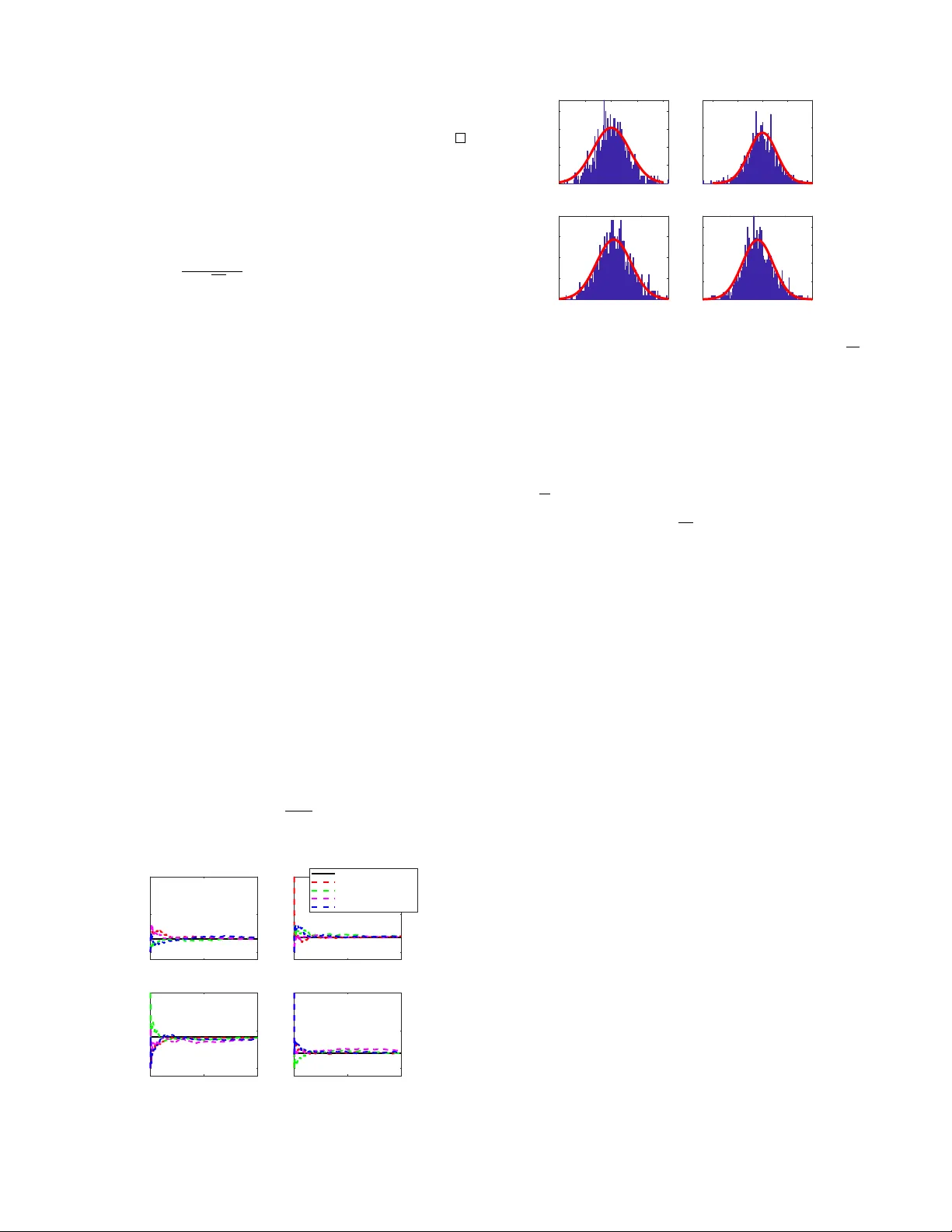
1 Asymptotic Pr operties of Distrib uted Social Sampling Algorithm Qian Liu, Xingkang He, Haitao Fang Social sampling is a novel randomized message passing pr o- tocol inspired by social communication f or opinion f ormation in social networks. In a typical social sampling algorithm, each agent holds a sample from the empirical distribution of social opinions at initial time, and it collaborates with other agents in a distributed manner to estimate the initial empirical distribution by randomly sampling a message from curr ent distribution estimate. In this paper , we focus on analyzing the theoretical properties of the distributed social sampling algorithm over random networks. Firstly , we provide a framework based on stochastic approximation to study the asymptotic properties of the algorithm. Then, under mild conditions, we prove that the estimates of all agents con verge to a common random distri- bution, which is composed of the initial empirical distribution and the accumulation of quantized error . Besides, by tuning algorithm parameters, we prov e the strong consistency , namely , the distribution estimates of agents almost surely conv erge to the initial empirical distribution. Furthermore, the asymptotic normality of estimation error generated by distributed social sampling algorithm is addressed. Finally , we provide a numerical simulation to validate the theoretical results of this paper . Index T erms —Social netw orks; opinion f ormation; social sam- pling; stochastic approximation; random networks; asymptotic normality I . I N T RO D U C T I O N In social networks, the study of opinion formation is to model the fragmentation or merging of opinions among agents in a society . A large class of real world phenomena can be well interpreted with opinion dynamics, such as election forecasting [1], analysis of public opinions [2], language ev olution [3] and so on. During the past decades, with the dev elopment of network technology and increasing of social communication, more and more researchers are focusing on the study of opinion formation in social networks as well as new approaches to distributed learning and estimation [4 – 10]. The results in sociology on opinion formation are mainly based on empirical studies, which usually lack sufficient theory foundation. Thus, in recent years, the requirements for mathematical modeling and theoretical analysis are increasing. Generally , in opinion dynamics, the communications between agents can be modeled by a network or a graph, whose edges represent channels through which one agent can share informa- tion with others. Naturally , the following issues are concerned: whether an equilibrium or consensus can be achiev ed via such social interactions? If the answer is yes, is this equilibrium Qian Liu and Haitao Fang are with LSC, Academy of Mathematics and Systems Science, Chinese Academy of Sciences, Beijing 100190, China; they are also with School of Mathematical Sciences, Univ ersity of Chinese Academy of Sciences, Beijing 100049, China. Xingkang He is with the Department of Automatic Control, KTH Royal Institute of T echnology , SE-100 44 Stockholm, Sweden. (xingkang@kth.se) influenced by network topology , initial opinions of agents or communication protocol? Otherwise, ho w can the opinion dynamics behav e? There are quite a few papers considering the above problems. The early work [11] proposes a common paradigm called Friedkin and Johnson model, where agents are divided into stubborn agents and regular agents. In [12], the Friedkin and Johnson model is viewed as a randomized gossip algorithm inducing oscillations, which should be er godic under some stable assumptions. Besides, a tractable communication model is developed in [13] to study the dynamics of belief formation and information aggregation. The authors propose asymptotic learning to describe that the fraction of agents can behave properly , and provide suf ficient and necessary conditions to guarantee the asymptotic learning. A continuous- time opinion dynamic model with stochastic gossip process is proposed in [14] to in vestigate the generation of disagreement and fluctuation. It is sho wn that the society containing stubborn agents with different opinions keeps fluctuating in an ergodic manner . Most of existing results focus on modeling the dynamics of consensus, diversity or fluctuation in social networks, where opinions are represented as scaler v ariables. A nature e xtension is that how the agents can obtain a common knowledge of the global phenomenon. In what follows, we discuss the local reconstruction of the empirical distribution of initial opinions via social interactions. In fact, probability distribution of opinions is a proper way to model the enormous opinions of agents on some certain subjects in a complex society , such as the election candidates they support or prefer . The aim of the agents is to estimate the discrete empirical distribution derived by the av erage of initial opinions through local interactions. This algorithm is essentially a randomized approximation of consensus procedure. So far , there have been a wide range of work on networked consensus in terms of communication noise, time delay , network topology and so on[15–20]. Nev- ertheless, due to the limitation of communication cost, each agent cannot exchange their entire opinions completely . T o deal with this problem, a communication scheme called social sampling is proposed [21]. The idea of this scheme is that each agent can only share a sample generated randomly by following its current distribution. The distributed social sam- pling algorithm giv en in [21] is a randomized approximation of consensus procedures, in which a group of agents aim to reach a common decision in a distributed way . Since the transferred message is quantized as an identical vector , the computation complexity is significantly reduced. Howe ver , the theoretical properties, such as the effects of network topology or the quantized process, hav e not been well inv estigated. Besides, one interesting theoretical problem is the asymptotic normality of estimation error . The work [22] considers such problem for 2 certain cases of noisy communication in consensus schemes for scalars and finds a connection between network topology and cov ariance matrix of the error limitation distribution. Howe ver , such a result cannot be transfered to distributed social sampling algorithm because of the quantized error term. In this paper, we will complete the analysis and establish asymptotic normality for the social sampling scenario. The main contributions of this paper are threefold: (i) W e provide a novel analysis framew ork based on stochastic approximation to study the asymptotic properties of the distributed social sampling algo- rithm ov er random networks. T o ensure the con- ver gence of the algorithm in an almost sure sense, we use the techniques of stochastic approximation [25], in which state space is decomposed into two parts: consensus part and v anishing part. Besides, some analysis methods provided in this paper can contribute to further related researches. (ii) For consensus over random networks, the strong consensus is most desirable. Compared with [21], this is achiev ed in our work under the milder condi- tions on network structures and communication noise properties. W e prove that the distribution estimates of agents reach consensus almost surely to the value related with true empirical distribution and the ac- cumulation of quantized error . Besides, by tuning al- gorithm parameters, we prove the strong consistency , i.e. , the distribution estimates of agents are almost surely conv ergent to the initial empirical distribution. On the other hand, unlike the fixed topology used in [21], the condition on network topology is relaxed to joint connectivity of mean digraphs for random networks. (iii) W e pro vide con vergence rate of estimation of the social sampling protocol. Explicitly , we prov e that the overall estimation errors of the algorithm are asymptotically normal with zero mean and known cov ariance matrix. The cov ariance matrix shows that how networks and quantized error influence the estimation performance of the distributed social sampling algorithm. Compared with [22], the condi- tions on communication noise in this work are more general. The reminder of the paper is organized as follows. Section II provides some preliminary information about graph theory and the main problem we considered. In section III , we describe the social sampling protocol and the stochastic algorithm studied in this paper . Con ver gence analysis for the distributed algorithm is giv en in section IV , while asymptotic properties are presented in section V . Section VI shows a numerical simulation. Section VII giv es some concluding remarks. A. Notations Let e i ∈ R M stand for the unit row vector whose i -th element equals to 1. I [ · ] denotes the indicator function and 1 stands for the proper dimensional column vector with elements all being 1. I N denotes the N -dimension identity matrix. The superscript “ T ” represents the transpose. The abbreviation i.i.d. stands for independent identically distrib ution of ran- dom variables, N (0 , S ) denotes the normal distribution with zero mean and covariance S . E [ x ] denotes the mathematical expectation of the stochastic variable x . Notation diag ( · ) represents the diagonalization of scalar elements. R n repre- sents the n -dimension Euclidean space. Besides, we denote [ N ] = { 1 , 2 , · · · , N } . I I . P R E L I M I NA R I E S A. Gr aph Theory Let G = ( V , E , W ) be a weighted digraph, where V = [ N ] is label set of N agents, E ⊂ V × V is the edge set, where an ordered pair ( i, j ) ∈ E means that agent i can get information from agent j directly . The in-neighbor set is denoted by N in ( i ) = { j ∈ V | ( i, j ) ∈ E } , while the out-neighbor set of agent i is denoted by N out ( i ) = { j ∈ V | ( j, i ) ∈ E } . The graph is undirected if it is bidirectional, i.e. ( j, i ) ∈ E if and only if ( i, j ) ∈ E . W = [ w ij ] ∈ R N × N is the weighted adjacency matrix of G , where w ij > 0 if ( i, j ) ∈ E , and w ij = 0 otherwise. The nonnegati ve matrix W is called row-wise stochastic if W1 = 1 , and is called column-wise stochastic if W T 1 = 1 . W e say W is double stochastic if it is both row-wise stochastic and column-wise stochastic. For any i, j ∈ [ N ] , the in-degree of agent i is defined as deg in ( i ) = P N j =1 w ij and the out-degree of agent i is defined as deg out ( i ) = P N j =1 w j i . W e say G is a balanced digraph, if deg in ( i ) = deg out ( i ) for any i ∈ [ N ] . The digraph G is strongly connected if for any pair i, j ∈ V , there exists a directed sequence of nodes i 1 , i 2 , . . . , i p ∈ V , such that ( i, i 1 ) ∈ E , ( i 1 , i 2 ) ∈ E , . . . , ( i p , j ) ∈ E . The network topology in this work is allowed to be time- varying, thus the weighted communication network at time k is denoted by G k = ( V , E k , W k ) . The graph sequence {G k } is called jointly connected, if there exists an integer T > 0 , such that  V , S T s =0 E s  is strongly connected. Besides, we introduce a definition to characterize the asymp- totic beha vior of the agents. Definition II.1 (Strong consensus [23]) . The estimates of agents ( i.e. Q i,k ) ar e said to reac h strong consensus if there exists a random variable q ∗ such that, with pr obability 1 and for all i ∈ [ N ] , lim k →∞ Q i,k = q ∗ . W e also say that the estimates con verg e almost surely ( a.s. ) . B. Distrib uted Learning of Distributions Consider a network of N agents. The communication relationship among agents is described by a sequence of directed graphs {G k } , where time is discrete and indexed by k = { 0 , 1 , 2 , . . . } . At initial time k = 0 , ev ery agent has a single discrete sample X i taking values in a finite state set χ = [ M ] . The problem we consider here is that agents in a network need to learn the empirical distribution Π , { Π ( x ) , x ∈ [ M ] } , where Π ( x ) = 1 N N X i =1 1 [ X i = x ] e x , ∀ x ∈ [ M ] = { 1 , 2 , . . . , M } . (1) 3 It can be considered as the histogram of the initial distribution of the agent opinions over the network. For illustration, we consider a motiv ating example. A group of customers who want to buy one product from M competing new products. Assume that ev ery customer has an opinion or preference over each product, which can be quantized as scores. T o get enough information, customers will communicate with their friends or neighbors about their opinions. In the traditional message protocol [4, 5, 7], the agents exchange their entire opinion histogram each time, which means customers will discuss the ev aluations of ev ery single product. This is not realistic, especially under the situation that there exist an enormous variety of products. A sample generated from the current estimate is transferred in social sampling protocol, which means customer simplifies the communication process and exchanges information about one kind of randomly selected product. The analysis of this paper shows that the customer still could get enough information about all products. I I I . P RO B L E M S E T U P A. Algorithm F ormulation In this paper , we aim to estimate this histogram through a randomized algorithm called social sampling [21]. The al- gorithm is based on the sample generated from the current estimate Q i,k of the true distribution Π . At time k , each agent holds an internal estimate Q i,k of Π with Q i, 0 = e X i . W e treat Q i,k as a probability distribution of the elementary vectors { e m : m ∈ [ M ] } , so that Q i,k should be probability vector on χ = [ M ] . Agent i generates its message social sample Y i,k as a function of the internal estimate Q i,k , then agent i sends Y i,k to its out-neighbors and receives the in-neighbor messages { Y j,k : j ∈ N i } . At each iteration, agent i uses the samples from its neighbors and current estimate to obtain the updated estimate Q i,k +1 . W e assume Y i,k ∈ Y = { e 1 , . . . , e M } , which can be viewed as a label of the opinion state space. So the opinion takes values from a finite, discrete value space. The random message Y i,k ∈ Y of agent i at time k is generated according to the distribution P i,k ∈ P ( Y ) , which is a function of the internal estimate Q i,k . More precisely , P i,k is a M - dimension ro w probability vector where the m -th element P m i,k = P ( Y i,k = e m ) . Remark III.1. W e can choose P i,k properly and make it be a correction term associated to the internal estimate Q i,k . For example, we set P i,k = 0 when Q i,k < α , where α is a presetting bound. Under some complicated situations, such as the opinion space being extremely lar ge or the histogram being far from uniform, this kind of censoring can av oid inefficient communication. Of course, we can also choose P i,k = Q i,k in some simple situations. Next, we will formulate the distributed social sampling algorithm and write it in a compact form. For notational con- venience, the social samples at time k are denoted by a N M - dimension column vector Y k ,  Y T 1 ,k , Y T 2 ,k , . . . , Y T N ,k  T ∈ R N M , which is generated from the sampling function P k ,  P T 1 ,k , P T 2 ,k , . . . , P T N ,k  T ∈ R N M . Similarly , we set Q k ,  Q T 1 ,k , Q T 2 ,k , . . . , Q T N ,k  T ∈ R N M . For agent i at time k , the internal estimate Q i,k is updated in a distributed way as follows: Q i,k +1 =  1 − δ k a k ii  Q i,k − δ k b k ii Y i,k + X j ∈N i ( k ) δ k w k ij Y j,k , (2) where a k ii , b k ii are communication coefficients subject to a k ii ≥ 0 , b k ii ≥ 0 . W k =  w k ij  ∈ R N × N is the weighted adjacency matrix of the network topology and δ k is the step size. By designing update procedure like this, we can add some reasonable assumptions on the coef ficients to guarantee that the internal estimate Q i,k +1 is a probability vector on the opinion state space χ = [ M ] at any time for every i ∈ [ N ] . This paper focuses on solving the following two problems: i) analyze the conditions ensuring the conv ergence of distributed social sampling algorithm (2) ov er random networks in the almost sure sense. ii) deriv e the asymptotic normality of algorithm (2) and characterize the effect of random sampling protocol and network topology on the limit cov ariance matrix. I V . C O N S E N S U S A N D C O N S I S T E N C Y In this section, we pro vide an analysis frame work based on stochastic approximation to study the con vergence of (2) . Denote A k , diag  a k 11 , · · · , a k N N  , B k , diag  b k 11 , · · · , b k N N  , then we can write (2) in a compact form Q k +1 = Q k + δ k  (( W k − B k − A k ) ⊗ I M ) Q k + (( W k − B k ) ⊗ I M ) ( Y k − Q k )  , (3) where “ ⊗ ” is the Kronecker product. Suppose that the σ -algebra F k , σ { Q i, 0 , W t , B t , 1 ≤ i ≤ N , 0 ≤ t ≤ k } is a filtration of the basic probability space (Ω , F , P ) . Hence Q k is measurable with respect to F k . Given the update rule in (3) , the consensus of the opinion dynamics is equiv alent to the con vergence of linear stochastic approximation algorithms. The linear matrix ( W k − B k − A k ) ⊗ I M represents the effect of network topology at time k , while (( W k − B k ) ⊗ I M ) ( Y k − Q k ) is the error item caused by the quantized data. As shown in iteration (3) , the opinion formation process can be considered as a linear regression case of stochastic approximation. Next, we will analyze (3) with stochastic approximation. T o begin with, the following assumptions are giv en. A1 δ k − − − − → k →∞ 0 , δ k > 0 , P ∞ k =0 δ k = ∞ , P ∞ k =0 δ 2 k < ∞ and 1 δ k +1 − 1 δ k − − − − → k →∞ δ ≥ 0 . A2 ( i ) { W k } k ≥ 0 is an independent random sequence with expectation denoted by ¯ W k = E [ W k ] and the adjacency matrix W k =  w k ij  is dou- ble stochastic. Besides, there exists an uniform bound ¯ w k ij > τ > 0 , ∀ k > 0 for all nonzero ¯ w k ij 6 = 0 . 4 ( ii ) There is an integer T > 0 , such that the mean graph ¯ G k =  V , E k , ¯ W k  generated by  ¯ W k  is jointly connected in the fixed period [ k , k + T ] , i.e. there exits an integer T > 0 , such that the graph  V , S T s =0 E {E k + s }  is strongly connected. In addition, we need extra assumptions on the mixed coef- ficients and the social sampling protocol. A3 k P k − Q k k 2 − − − − → k →∞ 0 , a.s. . A4 The communication coefficients a k ii and b k ii are cho- sen properly such that a k ii + b k ii = 1 for any k ≥ 0 , i.e. , A k + B k = I N . For con venience of analysis, we arrange the algorithm (3) as follo ws. Q k +1 = Q k + δ k  (( W k − I N ) ⊗ I M ) Q k + (( W k − B k ) ⊗ I M ) ( Y k − Q k )  = Q k + δ k   ¯ W k − I N  ⊗ I M  Q k +  ¯ W k − B k  ⊗ I M  ( P k − Q k ) +  W k − ¯ W k  ⊗ I M  P k + (( W k − B k ) ⊗ I M ) ( Y k − P k )  . (4) Denote        ¯ H k ,  ¯ W k − I N  ⊗ I M , C k ,  ¯ W k − B k  ⊗ I M  ( P k − Q k ) , M k , (( W k − B k ) ⊗ I M ) ( Y k − P k ) +  W k − ¯ W k  ⊗ I M  P k , (5) then we have Q k +1 = Q k + δ k  ¯ H k Q k + C k + M k  . (6) Remark IV .1. Condition A1 can be automatically satisfied if δ k = a k δ with a > 0 , δ ∈  1 2 , 1  . In fact, we can pick P k = Q k , i.e. , we generate social sample from internal estimate directly without censoring, which means C k = 0 . The double stochastic assumption on ¯ W k means that the mean graph should be balanced. The lo wer bound τ in A2 for the nonzero elements is used to guarantee the stability of linear matrix sequence { H k } , which is easily satisfied in the case where the network is switched over a finite number of network topologies. Before presenting the consensus results for the algorithm (6) , we provide the follo wing lemma. Lemma IV .1 (see [25]) . Let { H t } be n × n -matrices with sup t k H t k < ∞ . Assume that ther e is an n × n -matrix U > 0 and an integ er K > 0 such that for ∀ t ≥ 0 , U H t + H T t U ≤ 0 and t + K X s = t  U H T s + H s U  ≤ − β I n , β > 0 . If step-size { δ k } satisfies A1 and ω t can be expr essed as ω t = µ t + ν t wher e ∞ X t =1 δ t µ t +1 < ∞ and ν t − − − → t →∞ 0 , a.s.. Then, for an arbitrary initial value x 0 , the sequence { x t } generated by x t +1 = x t + δ t ( H t x t + ω t ) con verg es to zer o almost sur ely . Note that, in expression (6), we ha ve separated the quantized error into two parts: C k is a censoring item associated to the difference between the internal matrix Q k and the sampling matrix P k , and M k is a martingale dif ference sequence, which will be demonstrated in the following lemma. Lemma IV .2. ( M k , F k ) is a martingale differ ence sequence under A2 . Pr oof. See the proof in Appendix A. As claimed abov e, for the opinion dynamic consensus we only need to show the con vergence of Q k giv en by (6) almost surely . This is given by the following theorem. It is shown that all estimates of agents will achiev e consensus to a common estimate based on empirical distribution. Theorem IV .1 ( Consensus ) . Let { Q k } be generated by the algorithm (6) . Under the conditions A1 , A2 , A3 and A4 , we have lim k →∞ Q k = Q ∗ , a.s., (7) wher e Q ∗ = 1 ⊗ q ∗ . Explicitly , lim k →∞ Q i,k = q ∗ , a.s., where q ∗ ,  1 N 1 T ⊗ I M  Q 0 + 1 N ∞ X k =0 δ k  1 T ( W k − B k ) ⊗ I M  ( Y k − Q k ) , ∀ i ∈ [ N ] . Furthermor e, if k P k − Q k k = O ( δ k ) , then q ∗ < ∞ , a.s.. Pr oof. The mixed-product property of Kronecker product, ( A ⊗ B ) ( C ⊗ D ) = AC ⊗ B D , will be frequently used in the follo wing. Firstly , we write Q k as a sum of a vector in the consensus space and a disagreement vector by orthogonal decomposition. Let T ,  T 1 1 √ N 1 T  be an orthogonal matrix, then we have T 1 1 = 0 and T 1 T T 1 = I N − 1 . Set Γ , I N − 1 N 11 T , then T Γ =  T 1 0  . Pre-multiplying (3) by T Γ ⊗ I M yields  T 1 0  ⊗ I M  Q k +1 =  T 1 0  ⊗ I M  Q k + δ k   T 1 0  ⊗ I M  ¯ H k Q k +  T 1 0  ⊗ I M  C k +  T 1 0  ⊗ I M  M k  . (8) Setting ξ k , ( T 1 ⊗ I M ) Q k , we obtain ( T Γ ⊗ I M ) Q k =  ξ T k , 0  T , (9) 5 and ξ k +1 = ξ k + δ k  ( T 1 ⊗ I M ) {  ¯ W k − I N  ⊗ I M  ·  T T 1 ⊗ I M  ξ k + ( T 1 ⊗ I M ) ( C k + M k ) } = ξ k + δ k {  T 1  ¯ W k − I N  T T 1  ⊗ I M  ξ k + ( T 1 ⊗ I M ) C k + ( T 1 ⊗ I M ) M k } . (10) Denote F k , T 1  ¯ W k − I N  T T 1 = T 1 ¯ W k T T 1 − I N − 1 . T o use Lemma IV .1, we need to verify the stability of matrix sequence { F k ⊗ I M } . Since the adjacency matrix W k is double stochastic, i.e. , 1 T W k = 1 T and W k 1 = 1 , then ¯ W k has the single largest eigen value 1 by Perron’ s theorem [27]. Hence, ( ¯ W k + ¯ W T k ) 2 is a symmetric stochastic matrix which has the largest eigen value 1, and the eigen vector associated with 1 is 1 ∈ R N . No w , for any nonzero column vector z ∈ R N , z T ¯ W k z = z T  ¯ W k + ¯ W T k  2 z ≤ z T z . Moreov er , for any nonzero u ∈ R N − 1 , u  T 1 ¯ W k T T 1 − I N − 1  u T = ( uT 1 ) ¯ W k ( uT 1 ) T − ( uT 1 ) ( uT 1 ) T ≤ 0 . (11) Similarly , u  T 1 ¯ W T k T T 1 − I N − 1  u T = ( uT 1 ) ¯ W T k ( uT 1 ) T − ( uT 1 ) ( uT 1 ) T ≤ 0 . (12) By (11) –(12), it is easy to obtain that F k + F T k ≤ 0 . (13) V ia the jointly connectivity of the network defined in A2 , 1 T +1 P t + T s = t ¯ W s and 1 T +1 P t + T s = t ¯ W T s are irreducible double stochastic matrix. Then, for any z ∈ R N , it can obtain that z 1 2 ( T + 1) t + T X s = t  ¯ W s + ¯ W T s  ! z T − z z T ≤ 0 , where the equality holds if and only if z = c 1 . Since u T T 1 1 = 0 , u T T 1 can not be expressed as c 1 for any constant c . Consequently , for any nonzero u ∈ R N − 1 , the following strict inequality must hold:  u T T 1  1 2 ( T + 1) t + T X s = t  ¯ W s + ¯ W T s  !  u T T 1  T <  u T T 1   u T T 1  T . Notice T 1 T T 1 = I N − 1 , which implies that for any nonzero u ∈ R N − 1 , 1 2 ( T + 1) t + T X s = t u T  T 1  ¯ W s + ¯ W T s  T T 1 − 2 I N − 1  u < 0 . As a result, P t + T s = t  F s + F T s  < 0 . In addition, with the assumption on the uniform lower bound in A1 , there is a constant β > 0 such that t + T X s = t  F s + F T s  ≤ − β I N − 1 . (14) By (13) and (14), we hav e verified the conditions on linear matrix sequence { H t } in Lemma IV .1. Now , we analyze the noise term C k and M k in the iteration (6) . According to Lemma IV .2, M k is a martingale difference sequence, we obtain P ∞ k =0 δ k M k < ∞ , a.s. via the martingale con vergence theorem [26]. By assumption A3 , on the chosen scheme of correct function P k , we have that k C k k 2 (15) = ( P k − Q k ) T   ¯ W k − B k  T ⊗ I M   ¯ W k − B k  ⊗ I M  ( P k − Q k ) = ( P k − Q k ) T h  ¯ W k − B k  T  ¯ W k − B k   ⊗ I M i ( P k − Q k ) ≤ λ max n  ¯ W k − B k  T  ¯ W k − B k  ⊗ I M o k P k − Q k k 2 − − − − → k →∞ 0 , a.s.. Consequently , lim k →∞ C k = 0 , a.s.. In summary , we hav e verified all conditions in Lemma I V . 1 , then we can obtain lim k →∞ ( T Γ ⊗ I M ) Q k = lim k →∞  ξ T k , 0  T = 0 , a.s.. Note that T is an orthogonal matrix, so Γ ⊗ I M Q k − − − − → k →∞ 0 , a.s., where ( Γ ⊗ I M ) Q k =  I N − 1 N 11 T  ⊗ I M  Q k = Q k −  1 N 11 T ⊗ I M  Q k = Q k − ( 1 ⊗ I M )  1 N 1 T ⊗ I M  Q k = Q k − ( 1 ⊗ I M )   N X j =1 1 N Q j,k   , i.e. Q i,k − 1 N P N j =1 Q j,k − − − − → k →∞ 0 , a.s. for ev ery agent i ∈ [ N ] . Pre-multiplying update (6) by 1 N 1 T ⊗ I M yields  1 N 1 T ⊗ I M  Q k +1 (16) =  1 N 1 T ⊗ I M  Q k + δ k   1 N 1 T ⊗ I M   ¯ W k − I k  ⊗ I M Q k +  1 N 1 T ⊗ I M  ( C k + M k )  =  1 N 1 T ⊗ I M  Q k + δ k   1 N 1 T ⊗ I M  ( C k + M k )  , because row sum of the matrix ¯ W k − I N is zer o . Summing equation (16) from k = 0 to ∞ yields lim k →∞  1 N 1 T ⊗ I M  Q k +1 =  1 N 1 T ⊗ I M  Q 0 +  1 N 1 T ⊗ I M  ∞ X t =0 δ k ( C k + M k ) =  1 N 1 T ⊗ I M  Q 0 + 1 N ∞ X t =0 δ k  1 T ( W k − B k ) ⊗ I M  ( Y k − Q k ) 6 , q ∗ . Therefore, Q i,k − − − − → k →∞ q ∗ , a.s., ∀ i ∈ [ N ] . In the following, we will verify q ∗ < ∞ if k P k − Q k k = O ( δ k ) . Denote L 1 ,  1 N 1 T ⊗ I M  ∞ X k =1 δ k C k = 1 N ∞ X k =1 δ k  1 T  ¯ W k − B k  ⊗ I M  ( P k − Q k ) , (17) L 2 ,  1 N 1 T ⊗ I M  ∞ X k =1 δ k M k , (18) then, due to k P k − Q k k = O ( δ k ) and A1 , we hav e k L 1 k = k 1 N ∞ X k =1 δ k  1 T  ¯ W k − B k  ⊗ I M  ( P k − Q k ) k ≤ 1 N ∞ X k =1 δ k k  1 T  ¯ W k − B k  ⊗ I M  k · k ( P k − Q k ) k ≤ M N ∞ X k =1 δ 2 k < ∞ . (19) In addition, we ha ve known that { M k , F k } is a martingale difference sequence [26] in Lemma IV .2, thus P ∞ k =0 δ k M k < ∞ , i.e. L 2 < ∞ . In conclusion, q ∗ < ∞ . Corollary 1. ( Strong consistency ) Let B k ≡ I N and A1 − A4 hold, then { Q k } generated by (6) conver ges to the true distrib ution, i.e. lim k →∞ ( Q i,k − Q j,k ) = 0 , ∀ i, j ∈ [ N ] , a.s., lim k →∞ Q i,k = q ∗ ,  1 N 1 T ⊗ I M  Q 0 , a.s.. Remark IV .2. Compared with the undirected graph in [21], the joint connectivity of directed graph pointed at A2 in Theorem IV .1 is a weaker condition. Besides, we have deriv ed strong consensus to a finite limit q ∗ , which is almost identical with the true distribution Π . V . A S Y M P T OT I C N O R M A L I T Y In this section, we will establish asymptotic normality for estimate error Q k − Q ∗ of the distributed social sampling algorithm. The main tool for asymptotic normality analysis is shown in the following lemma. Lemma V .1 (Theorem 3.3.1 in [24]) . Let H k and H be l × l -matrices, { x k } be given by x k +1 = x k + δ k ( H k x k + e k +1 + v k +1 ) with an arbitrarily given initial value. Assume that the step-size δ k satisfies A1 and the following conditions hold C1 H k − − − − → k →∞ H and H + δ 2 I is stable with the constant δ given in A1 ; C2 v k = o  √ δ k  ; C3 { e k , F k } is a martingale differ ence sequence of l - dimension which satisfies E ( e k |F k − 1 ) = 0 and sup k E  k e k k 2 |F k − 1  ≤ σ with σ being a constant , lim k →∞ E  e k e T k |F k − 1  = lim k →∞ E e k e T k , S 0 , a.s., lim N →∞ sup k E k e k k 2 I [ k e k k >N ] = 0 , then x k √ δ k d − − − − → k →∞ N (0 , S ) , wher e S = Z ∞ 0 e ( H + δ 2 I ) t S 0 e ( H T + δ 2 I ) t dt. For the case where the root set of the observ ation function f ( x ) = ¯ H k ( x ) consists of a singleton z er o , we consider { ξ k } which is defined in (10) . It has been verified that lim k →∞ ξ k = 0 , a.s. . Re write (10) as ξ k +1 = ξ k + δ k { ( T 1 ⊗ I M ) ¯ H k  T T 1 ⊗ I M  ξ k + ( T 1 ⊗ I M ) ( C k + M k ) } , (20) where ¯ H k , C k and M k are gi ven by (5) . It can be seen that ξ k is updated by a linear stochastic approximation algorithm to approach the sought root z er o . Furthermore, we can inv es- tigate the asymptotic properties of (20) . Before describing the con vergent rate of iteration (20) , we require the following assumptions. W e keep A1 unchanged, but strengthen A3 to A3 0 and change A2 to A2 0 as follows. A2 0 ( i ) { W k } is an i.i.d. sequence. ( ii ) The mean graph ¯ G k =  V , E k , ¯ W  generated by ¯ W = E [ W k ] is strongly connected and the adjacency matrix W k is double stochastic. A3 0 k P k − Q k k = o ( δ k ) . A4 0 Choose B k ≡ B , where B is a constant matrix. A5 For sampling Y k under distribution P k , we assume that Σ is a constant matrix almost surely , where Σ , lim k →∞ E h ( Y k − P k ) ( Y k − P k ) T |F k − 1 i . Remark V .1. W e consider an example of A5 for il- lustration. Recall that the random message Y k ,  Y T 1 ,k , Y T 2 ,k , · · · , Y T N ,k  T is generated from the sampling func- tion P k ,  P T 1 ,k , P T 2 ,k , · · · , P T N ,k  T . Let Y i,k = e m with probability P m i,k , where m ∈ [ M ] . Then Σ k , E h ( Y k − P k ) ( Y k − P k ) T |F k − 1 i =      Σ 1 ,k 0 · · · 0 0 Σ 2 ,k · · · 0 . . . . . . . . . . . . 0 0 · · · Σ N ,k      , (21) where Σ i,k = E h ( Y i,k − P i,k ) ( Y i,k − P i,k ) T |F k − 1 i =       1 − P 1 i,k  P 1 i,k · · · 0 . . . . . . . . . 0 · · ·  1 − P M i,k  P M i,k      . From P k − Q k − − − − → k →∞ 0 a.s. , Q k − Q ∗ − − − − → k →∞ 0 a.s. , we hav e Σ k − − − − → k →∞ Σ = { ( I M − diag ( q ∗ )) diag ( q ∗ ) } ⊗ I N . 7 The following lemma considers the martingale dif ference sequence part. Lemma V .2. Under A2 0 and A4 0 , by choosing B ≡ I N , we have ε k , ( T 1 ⊗ I M ) M k = ( T 1 ( W k − B ) ⊗ I M ) ( Y k − P k ) +  T 1  W k − ¯ W  ⊗ I M  P k (22) is a martingale differ ence sequence satisfying E ( ε k |F k − 1 ) = 0 , sup k E  k ε k k 2 |F k − 1  ≤ σ with σ being a constant, (23) lim N →∞ sup k E k ε k k 2 I [ k ε k k >N ] = 0 . (24) Pr oof. See the proof in Appendix B. Now we can establish the asymptotic normality of the distributed social sampling algorithm (20) . Theorem V .1 ( Asymptotic normality ) . Let A1 , A2 0 , A3 0 , A4 0 and A5 hold, then ξ k = ( T 1 ⊗ I M ) Q k is asymptotically normal, i.e. the distribution of 1 √ δ k ξ k con verg e to a normal distribution: ξ k √ δ k d − − − − → k →∞ N ( 0 , S ) , (25) wher e S = Z ∞ 0 e ( ¯ F + δ 2 I ( N − 1) M ) t S 0 e ( ¯ F + δ 2 I ( N − 1) M ) T t dt, S 0 , E [( T 1 ( W k − I N ) ⊗ I M )] Σ E h ( W k − I N ) T T T 1 ⊗ I M i , ¯ F ,  T 1  ¯ W − I N  T T 1  ⊗ I M , Σ , lim k →∞ E h ( Y k − P k ) ( Y k − P k ) T |F k − 1 i . Pr oof. T o use Lemma V . 1 , we hav e to validate conditions C1 and C2. First, we consider C1. Denote ¯ F k , ( T 1 ⊗ I M ) ¯ H k  T T 1 ⊗ I M  , by A2 0 on the weighted matrix W k , we have ¯ F + δ 2 I ( N − 1) M = ( T 1 ⊗ I M )  ¯ W − I N  ⊗ I M   T T 1 ⊗ I M  + δ 2 I ( N − 1) M =  T 1  ¯ W − I N  T T 1  ⊗ I M + δ 2 I ( N − 1) M . Under assumption A2 0 , ¯ W = E [ W k ] is a stochastic matrix and its largest eigen value is 1 via Perron’ s Theorem [27]. Let the second largest eigen value of ¯ W be λ 2 . W e can choose step-size δ k properly such that λ 2 < 1 − δ 2 , where the linear matrix in (20) satisfies the stable assumption in C1. Now we analyze C2 item by item. First v k , ( T 1 ⊗ I M ) C k , where C k is defined in (5) . W e can obtain v k = o ( δ k ) according to A3 0 and (15) . According to (22) , the martingale difference part of noise has ε k ε T k =  T 1  W k − ¯ W  ⊗ I M  P k P T k   W k − ¯ W  T T T 1 ⊗ I M  +  T 1  W k − ¯ W  ⊗ I M  P k ( Y k − P k ) T ·  ( W k − I N ) T T T 1 ⊗ I M  + ( T 1 ( W k − I N ) ⊗ I M ) ( Y k − P k ) P T k ·   W k − ¯ W  T T T 1 ⊗ I M  + ( T 1 ( W k − I N ) ⊗ I M ) ( Y k − P k ) · ( Y k − P k ) T  ( W k − I N ) T T T 1 ⊗ I M  , S 1 + S 2 + S 3 + S 4 . Notice that  T 1  W k − ¯ W  ⊗ I M  P k =  T 1  W k − ¯ W  ⊗ I M  ( P k − Q k ) +  T 1  W k − ¯ W  ⊗ I M  ( Q k − Q ∗ ) +  T 1  W k − ¯ W  ⊗ I M  Q ∗ =  T 1  W k − ¯ W  ⊗ I M  ( P k − Q k ) +  T 1  W k − ¯ W  ⊗ I M  ( Q k − Q ∗ ) +  T 1  W k − ¯ W  ⊗ I M   1 ⊗  1 N 1 T ⊗ I M Q 0  =  T 1  W k − ¯ W  ⊗ I M  ( P k − Q k ) +  T 1  W k − ¯ W  ⊗ I M  ( Q k − Q ∗ ) +  T 1  W k − ¯ W  1  ⊗  1 N I M  1 T ⊗ I M  Q 0  . Since W k and ¯ W all are double stochastic matrix and k P k − Q k k − − − − → k →∞ 0 , a.s. , Q k − Q ∗ − − − − → k →∞ 0 , a.s. , we have  T 1  W k − ¯ W  ⊗ I M  P k − − − − → k →∞ 0 , a.s.. (26) Therefore, we can obtain lim k →∞ E [ S 1 |F k − 1 ] = 0 , a.s. , lim k →∞ E [ S 2 |F k − 1 ] = 0 , a.s. and lim k →∞ E [ S 3 |F k − 1 ] = 0 , a.s. . On the other hand, due to A5 , Σ , lim k →∞ E h ( Y k − P k ) ( Y k − P k ) T |F k − 1 i is a constant matrix almost surely . Besides, W k is independent with F k − 1 in A2 0 , then lim k →∞ E { S 4 |F k − 1 } = lim k →∞ E { ( T 1 ( W k − I N ) ⊗ I M ) ( Y k − P k ) ( Y k − P k ) T  ( W k − I N ) T T T 1 ⊗ I M  |F k − 1 } = lim k →∞ E { E { ( T 1 ( W k − I N ) ⊗ I M ) ( Y k − P k ) ( Y k − P k ) T  ( W k − I N ) T T T 1 ⊗ I M  |F k − 1 , W k }|F k − 1 } = lim k →∞ E { ( T 1 ( W k − I N ) ⊗ I M ) E { ( Y k − P k ) ( Y k − P k ) T |F k − 1 , W k }  ( W k − I N ) T T T 1 ⊗ I M  |F k − 1 } = lim k →∞ E { ( T 1 ( W k − I N ) ⊗ I M ) |F k − 1 } E { E { ( Y k − P k ) ( Y k − P k ) T |F k − 1 , W k }|F k − 1 } × E { ( W k − I N ) T T T 1 ⊗ I M |F k − 1 } = E { ( T 1 ( W k − I N ) ⊗ I M ) } · Σ · E { ( W k − I N ) T T T 1 ⊗ I M } , S 0 . 8 According to Lemma V .2, we have verified C2. In summary , we have verified all conditions in Lemma V .1, thus conclusion of this theorem holds. Corollary 2. Suppose A1 , A2 0 , A3 0 , A4 0 and A5 hold, then Q k − Q ∗ √ δ k d − − − − → k →∞ N  0 , e S  , wher e e S , ( T Γ ⊗ I M ) T  S 0 0 0  ( T Γ ⊗ I M ) . Remark V .2. Theorem V .1 and Cor ollary 2 establish that the error between estimates generated by algorithm (3) and true empirical distribution is asymptotically normal, and the asymptotic covariance is char acterized by network topology and quantized protocol. Our analysis results ar e more detailed and pr ofound than that in [21], which only gives bounds on the e xpected squar ed err or . V I . N U M E R I C A L S I M U L A T I O N In this section we provide a numerical simulation for the distribution social sampling algorithm considered in (2) . Let N = 50 with the underlying graph being fully connected. Each agent holds an initial opinion Q i, 0 = e X i , which is drawn i.i.d. from [0 . 2 0 . 3 0 . 4 0 . 1] . It means that the dimension of opinion state space M = 4 . At each time k , agent i generates its random message Y i,k ∈ { e 1 , e 2 , e 3 , e 4 } based on the internal estimate Q i,k directly , i.e. , we choose P i,k = Q i,k and do not make corrections. Setting the mixed coefficients a k ii = 0 , b k ii = 1 , step size δ k = 1 k 0 . 75 , we update the internal estimate sequence { Q i,k } according to iteration (2) . 0 500 1000 k 0 0.5 1 0 500 1000 k 0 0.5 1 0 500 1000 k 0 0.5 1 0 500 1000 k 0 0.5 1 Initial Emperical Distribution Estimates of Node 5 Estimates of Node 6 Estimates of Node 10 Estimates of Node 24 Figure 1: Trace of estimate of Q i,k for i ∈ [ N ] over every single opinion state m ∈ [ M ] with M = 4 -1 -0.5 0 0.5 1 0 5 10 15 20 Node 5 -1 -0.5 0 0.5 1 0 10 20 30 Node 6 -1 -0.5 0 0.5 1 0 5 10 15 20 Node 10 -1 -0.5 0 0.5 1 0 5 10 15 20 Node 24 Figure 2: Histogram and limit distribution for ( Q i,k − q ∗ ) / √ δ k at k = 500 . The trace of estimate sequence of empirical distribution Π for some selected agents is shown in Figure 1, where each subgraph presents a state in [ M ] = 4 . As shown in Theorem IV .1, the estimated sequence generated by social sampling procedure con verges to the true empirical distrib ution q ∗ ,  1 N 1 T ⊗ I M  Q 0 . W e have calculated the algorithm (2) for 1000 times independently . The histograms for each component of ( Q i,k − q ∗ ) / √ δ k at k = 500 are shown in Figure 2. It is sho wn that the data fits the normal distribution well. V I I . C O N C L U S I O N S In this work, conv ergence of distrib uted social sampling algorithm toward a common distribution has been established ov er random networks based on stochastic approximation. W e ha ve proved that the distribution estimates deriv ed by agents’ local interaction reached consensus almost sure to a value, which is related with the true empirical distribution and accumulation of quantized error . Furthermore, the error between estimates and true empirical distribution has been shown to be asymptotically normal with zero mean and known cov ariance, which is characterized by network topology and the social sampling protocol. In fact, the randomized sample procedure is fairly general to be used in other problems, such as distributed optimization ov er large data sets. As the messages are quantized as identical vectors, the computation complexity is significantly reduced. In the future work, we will dig deeper about this random message passing protocol. R E F E R E N C E S [1] Holle y R A, Liggett T M. Ergodic theorems for weakly interacting infinite systems and the voter model. Annals of Probability , 1975, 3 (4):643–663 [2] Acemoglu D, Dahleh M A, Lobel I, et al. Bayesian learning in social networks. The Revie w of Economic Studies, 2011, 78(4): 1201–1236 [3] Narayanan H, Niyogi P . Language ev olution, coalescent processes, and the consensus problem on a social net- work. Journal of Mathematical Psychology , 2014, 61:19– 24 9 [4] He gselmann R, Krause U. Opinion dynamics and bounded confidence models, analysis, and simulation. Journal of Artificial Societies and Social Simulation, 2002, 5(3):1–33 [5] Boyd S, Ghosh A, Prabhakar B, et al. Randomized gossip algorithms. IEEE Transactions on Information Theory , 2006, 52(6): 2508–2530 [6] Pineda M, T oral R, Hernandez-Garcia E. Noisy continuous-opinion dynamics. Journal of Statistical Mechanics: Theory and Experiment, 2009, 2009(08): P08001 [7] Zhang J, Hong Y . Opinion ev olution analysis for short- range and long-range Deffuant-W eisbuch models. Phys- ical A Statistical Mechanics & Its Applications, 2013, 392(21):5289–5297 [8] Frasca P , Ishii H, Ra vazzi C, et al. Distributed ran- domized algorithms for opinion formation, centrality computation and power systems estimation: A tutorial ov erview . European Journal of Control, 2015, 24(1): 2– 13 [9] Friedkin N E, Proskurnikov A V , T empo R, et al. Network science on belief system dynamics under logic constraints. Science, 2016, 354(6310):321–326 [10] Lou Y , Strub M, Li D, et al. Reference Point F ormation in Social Networks, W ealth Growth, and Inequality . Social Science Electronic Publishing, 2017 [11] Friedkin N E, Johnsen E C. Social Influence Networks and Opinion Change. Advances in Group Processes, 1999, 16:1–29 [12] Ra vazzi C, Frasca P , T empo R, et al. Ergodic randomized algorithms and dynamics ov er networks. IEEE Transac- tions on Control of Network Systems, 2015, 2(1): 78–87 [13] Acemoglu D, Bimpikis K, Ozdaglar A. Dynamics of information exchange in endogenous social networks. Theoretical Economics, 2014, 9(1): 41–97 [14] Acemoglu D, Como G, Fagnani F , et al. Opinion fluctu- ations and disagreement in social networks. Mathematics of Operations Research, 2013, 38(1): 1–27 [15] De groot M H. Reaching a Consensus. Journal of the American Statistical Association, 1974, 69(345):118–121 [16] Borkar V , V araiya P P . Asymptotic agreement in dis- tributed estimation. IEEE T ransactions on Automatic Control, 1982, 27(3):650–655 [17] Tsitsiklis J N, Athans M. Conv ergence and asymptotic agreement in distributed decision problems. IEEE Con- ference on Decision and Control, 1983:692–701 [18] Olfati-saber R, Murray R M. Consensus problems in networks of agents with switching topology and time- delays. IEEE Transactions on Automatic Control, 2004, 49(9):1520–1533 [19] Imai Y , Kohsaka S. Distributed Consensus Algorithms in Sensor Networks W ith Imperfect Communication: Link Failures and Channel Noise. IEEE T ransactions on Signal Processing, 2009, 57(1):355–369 [20] Leblanc H J, Zhang H, Koutsoukos X, et al. Re- silient Asymptotic Consensus in Robust Networks. IEEE Journal on Selected Areas in Communications, 2013, 31(4):766–781 [21] Sarwate A D, Ja vidi T . Distributed Learning of Dis- tributions via Social Sampling. IEEE Transactions on Automatic Control, 2015, 60(1):34–45 [22] Rajagopal R, W ainwright M J. Network-Based Con- sensus A veraging W ith General Noisy Channels. IEEE T ransactions on Signal Processing, 2011, 59(1):373–385. [23] Huang M, Manton J H. Coordination and consensus of networked agents with noisy measurements: stochastic algorithms and asymptotic behavior . SIAM Journal on Control and Optimization, 2009, 48(1): 134–161 [24] Chen H F . Stochastic approximation and its applications. Springer Science & Business Media, 2006 [25] F ang H, Chen H F , W en L. On control of strong consen- sus for netw orked agents with noisy observ ations. Journal of Systems Science and Complexity , 2012, 25(1): 1–12 [26] Durrett R. Probability: theory and examples. Cambridge Univ ersity Press, 2010 [27] Me yer , Carl D. Matrix analysis and applied linear alge- bra. SIAM, 2000 A P P E N D I X Appendix A Pr oof of Lemma IV .2 According to the protocol of social sampling, we hav e E [ Y i,k ] = P M m =1 P ( Y i,k = e m ) = P M m =1 e m P m i,k = P i,k . Thus, E [ Y k ] = P k . T aking conditional expectation gi ven F k − 1 ov er both sides of (5) , we obtain E [ M k |F k − 1 ] = E [(( W k − B k ) ⊗ I M ) ( Y k − P k ) |F k − 1 ] + E  W k − ¯ W k  ⊗ I M  P k |F k − 1  = E [( W k − B k ) ⊗ I M ] E [( Y k − P k ) |F k − 1 ] + E  W k − ¯ W k  ⊗ I M  P k = 0 . Hence, { M k , F k } is a martingale difference sequence. Appendix B Pr oof of Lemma V .2 Since we hav e verified that ( M k , F k ) is a martingale difference sequence and T 1 is a constant matrix, ( ε k , F k ) giv en by (22) is also a martingale difference sequence. At first, we demonstrate the boundedness of ε k . The random message Y i,k ∈ Y = { 0 , e 1 , · · · , e M } of agent i at time k is generated according to the M -dimension row probability vector P i,k ∈ P ( Y ) . Besides, W k is a double stochastic matrix by A2 0 , then we obtain k ε k k ≤k ( T 1 ⊗ I M ) (( W k − I N ) ⊗ I M ) ( Y k − P k ) k + k ( T 1 ⊗ I M )  W k − ¯ W  ⊗ I M  P k k ≤k T 1 ⊗ I M k · k ( W k − I N ) ⊗ I M k · k Y k − P k k + k T 1 ⊗ I M k · k  W k − ¯ W  ⊗ I M k · k P k k ≤ cN 2 M 2 . Hence, the noise sequence ε k is bounded. W e can derive (23) and (24) directly .