Adaptive backstepping control for FOS with nonsmooth nonlinearities

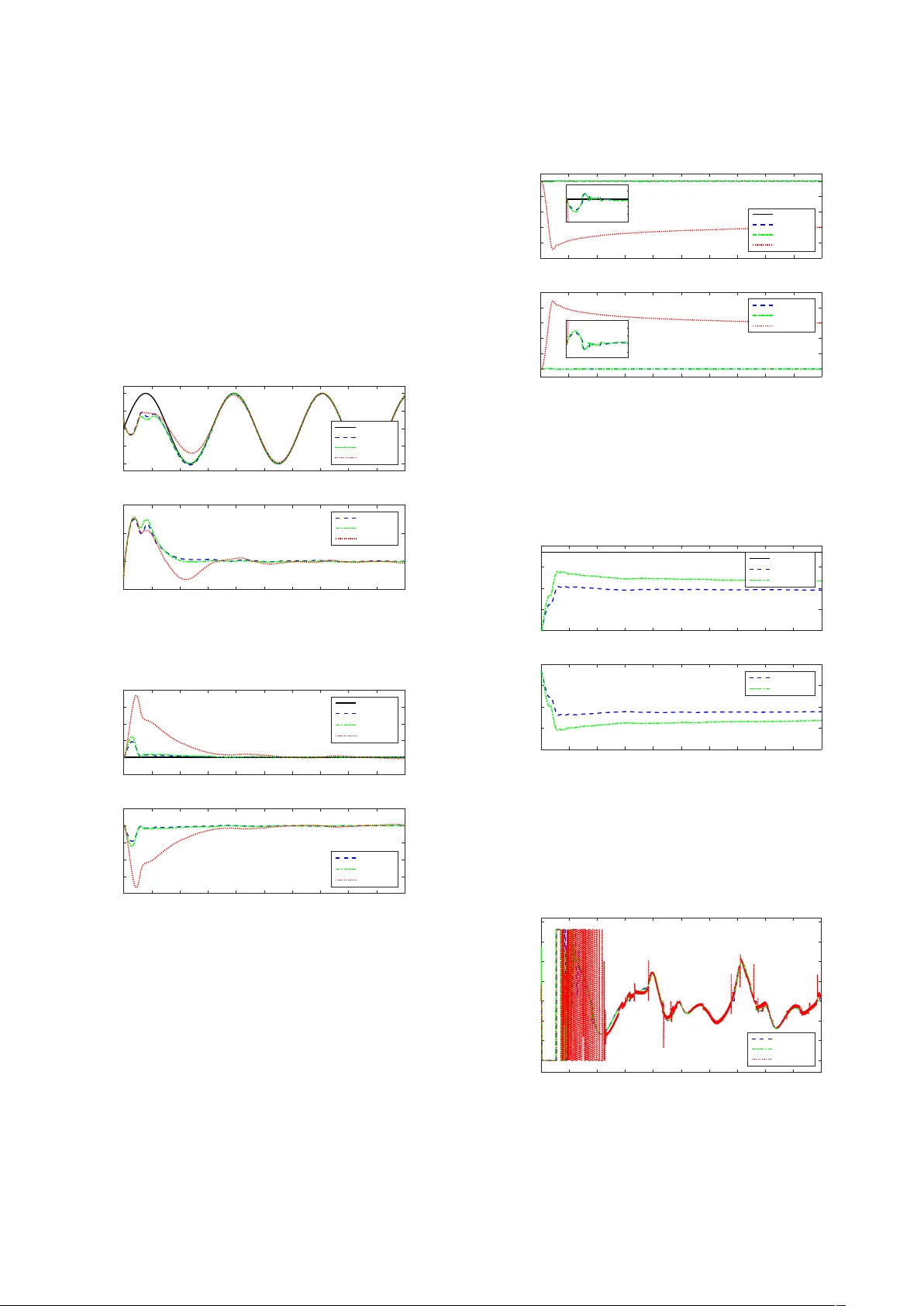
Adapti ve backstepping control for FOS with nonsmooth nonlinearities Dian Sheng , Y iheng W ei , Songsong Cheng , Y ong W ang ∗ Department of Automation, University of Science and T echnology of China, Hefei, 230026, China Abstract This paper proposes an original solution to input saturation and dead zone of fractional order system. T o o vercome these nonsmooth nonlinearities, the control input is decomposed into two independent parts by introducing an intermediate variable, and thus the problem of dead zone and saturation transforms into the problem of disturbance and saturation afterwards. W ith the procedure of fractional order adaptiv e backstepping controller design, the bound of disturbance is estimated, and saturation is compensated by the virtual signal of an auxiliary system as well. In spite of the existence of nonsmooth nonlinearities, the output is guaranteed to track the reference signal asymptotically on the basis of our proposed method. Some simulation studies are carried out in order to demonstrate the e ff ectiv eness of method at last. K e ywor ds: Fractional order systems; Adaptiv e backstepping control; Nonsmooth nonlinearities; Dead zone; Saturation 1. Introduction When we deal with practical control problems, it is in- evitable to face the troubles caused by the presence of real physical components, which often contains nonsmooth non- linearities [1]. Nonsmooth nonlinearities always lead to such unexpected result that they have become an independent and new field of research. Of all kinds of nonsmooth nonlin- earities, the saturation and dead zone are the most common and significant since almost all actuators are enslaved to such two nonlinearities to some extent. As a static input-output characteristic, dead zone often appears in gears [2, 3], valv es [4], motors [5], robot arms [6] and e ven ele vators of aircraft [7]. As for saturation, the motor speed is limited due to physical constraints, the output of the operational amplifier won’t be larger than its supply voltage and the finite word length results in ov erflow in computer . W ith the purpose of compensating dead zone and saturation, many scholars are dedicated to these nonlinearities and obtain abundant results [8–11]. Be that as it may , when it comes to fractional order systems (FOS), there are few results about ho w to deal with dead zone and saturation. As is known to all, fractional order system and control dev elop rapidly during last decades. There are two factors that lead to this prosperity . First, fractional order calculus could describe man y engineering plants and processes pre- cisely . The second factor is the superiority of fractional order controllers, i.e., design freedom and rob ust ability [12 – 16]. Therefore, a large number of exciting results about FOS such as stability analysis [17 – 19], controllability and observability [20], signal processing [21], numerical computation [22 – 24], system identification [25, 26] and controller synthesis [27] hav e been achie ved. As the FOS dev elop, some potential problems, ∗ Y ong W ang is the corresponding author . Email addr ess: yongwang@ustc.edu.cn (Y ong W ang) especially dead zone and saturation, which were once ignored, gradually attract the attention of scholars now . Although great e ff orts hav e been made to control FOS with dead zone and saturation, there are still few v aluable results so far . Machodo reveals the superior performance of fractional order controller in the control of systems with nonlinear phenomena and proves it separately in the presence of saturation, dead zone, hysteresis and relay [28]. By exploiting the saturation function with sector bounded condition, Lim puts forward a method that makes fractional order linear systems with input saturation asymptotically stable [29]. Based on t − α asymptotical stability , Shahri analyzes the stability of the same system by means of direct L yapunov method [30]. In recent paper [31], Shahri also studies the similar problem but disturbance rejection is taken into consideration this time. Considering both their works on linear system, Luo lately discusses the saturation problem of nonlinear FOS [32]. In the case of FOS with dead zone, sliding mode control and switching adaptive control hav e been applied by confining the control input to a sector area [33 – 35]. The indirect L yapunov method is introduced to control fractional order micro electro mechanical resonator with dead-zone input [36]. Even if some significant works have been done, it’ s still far from perfection. There remains room to improv e current research. • Dead zone and saturation are studied separately while they often take e ff ect at the same time. • The form of dead zone and saturation should not be confined. • The order of the FOS could be extended to incommensu- rate one. • In addition to stabilization, the goal of tracking is sup- posed to be achiev ed. Pr eprint submitted to IF AC J ournal of Systems and Contr ol December 20, 2024 • The uncertain nonlinear FOS deserves deeply research- ing. • External disturbance cannot be ignored in reality . Therefore, this paper proposes a control method for uncer - tain nonlinear incommensurate FOS in the presence of dead zone and saturation. T o the best of our knowledge, no scholar has e ver in vestigated the input saturation and dead zone of FOS simultaneously . Our proposed method is creativ e and original not only in FOS b ut also integer order systems. First, by introducing intermediate variable, the input saturation and dead zone are decomposed into two independent parts where the dead zone part needs decomposing further . Thus the problem of input saturation and dead zone is transformed into the the problem of input saturation and bounded disturbance. Second, a fractional order auxiliary system is constructed to generate virtual signals which are used for compensating saturation. Third, based on fractional order adaptive backstepping control (FO ABC) [37 – 40], the objective of tracking reference signal has been achie ved in the end. Considering not all parameters of input saturation and dead zone a vailable in practice, the entirely unknown case of nonsmooth nonlinearities is seriously studied as well. The remainder of this article is organized as follows. Sec- tion 2 introduces the problem formulation and provides some basic knowledge for subsequent use. After model transforma- tion and input decomposition, adaptiv e backstepping control strategy is recommended for the known and unknown cases of parameters in Section 3. In Section 4, simulation results are provided to illustrate the v alidity of the proposed approach. Conclusions are giv en in Section 5. 2. Preliminaries Let us consider the following parameter strict-feedback of uncertain nonlinear incommensurate FOS with nonsmooth nonlinearities and disturbance                D α i x i = d i x i + 1 + ψ i ( x 1 , x 2 , · · · , x i ) + ϕ T i ( x 1 , x 2 , · · · , x i ) θ, i = 1 , · · · , n − 1 , D α n x n = bu ( v ) + ψ n ( x ) + ϕ T n ( x ) θ + d , y = x 1 , (1) where 0 < α i < 1 ( i = 1 , · · · , n ) are the system incommensurate fractional order , θ ∈ R q is a constant and unknown vector , b is the input coe ffi cient, d i ( i = 1 , · · · , n − 1) are known nonzero real constants, ψ i ( · ) ∈ R and ϕ i ( · ) ∈ R q ( i = 1 , · · · , n ) are known nonlinear functions, x = [ x 1 · · · x n ] T ∈ R n is the pseudo system state vector , and d is the time-v arying disturbance within unknown bound | d | < D . u ( v ) ∈ R represents the actual control input restrained by dead zone as well as saturation, and v ∈ R is the desired control input, namely , u =                    U u p , v ( t ) ≥ w M , m [ v ( t ) − b r ] , b r ≤ v ( t ) < w M , 0 , b l < v ( t ) < b r , m [ v ( t ) − b l ] , w m < v ( t ) ≤ b l , U low , v ( t ) ≤ w m , (2) with w M = U u p m + b r and w m = U low m + b l . The slope m is possibly known, but the parameters of such nonsmooth nonlinear input, U u p , U low , b l , b r , are entirely unknown. If slope m is unknown, all parameters of dead zone and saturation are unknown as well, which leads to a big trouble that we will study later . T o sho w the relationship between u and v visually , the phase diagram is drawn in Fig 1. up U low U r b l b M w m w v u Fig. 1. Control input subject to dead zone and saturation. The objectiv e of this study is to develop an e ff ecti ve ap- proach to enable the output y to track the reference signal r asymptotically under the following assumptions. Assumption 1. The sign of input coe ffi cient sgn( b ) is known. Assumption 2. The r efer ence signal r and its first l P j i = 1 α i m -th or der derivatives ar e piecewise continuous and bounded, j = 1 , · · · , n. There are three widely accepted definitions of fractional order deri vati ve D α , but the Caputo’ s one is chosen for sub- sequent use due to some good properties, namely its deriv ativ e of constant equals zero and there’ s no need to calculate frac- tional order deri vati ve of initial value when operating Laplace transformation. The Caputo’ s definition is c D α t f ( t ) = 1 Γ ( m − α ) R t c f ( m ) ( τ ) ( t − τ ) α − m + 1 d τ, (3) where m − 1 < α < m , m ∈ N + , Γ ( α ) = R ∞ 0 x α − 1 e − x d x is the Gamma function. On the basis of Caputo’ s definition, the ne xt additi ve la w of exponents holds on condition that f ( c ) = 0 and 0 < p , q < 1 c D p t  c D q t f ( t )  = c D q t  c D p t f ( t )  = c D p + q t f ( t ) . (4) For purpose of con venient expression, the α order deriv ativ e from initial time zero 0 D α t is simplified as D α . Just before un- cov ering the main results, some helpful lemmas need referring. Lemma 1. (see [41]) The di ff er ential equation D α y ( t ) = u ( t ) with fractional order 0 < α < 1 , y ( t ) ∈ R and u ( t ) ∈ R can be transformed into the following linear continuous fr equency distributed model ( ∂ z ( ω, t ) ∂ t = − ω z ( ω, t ) + u ( t ) , y ( t ) = R ∞ 0 µ α ( ω ) z ( ω, t ) d ω, (5) wher e µ α ( ω ) = ω − α sin ( απ ) / π and z ( ω, t ) ∈ R is the true state of the system. Remark 1. The Lemma 1 implies the infinite dimension of fractional order state. And this lemma derives from zero initial 2 condition, while the system response by definition of Riemann- Liouville or Caputo corresponds to the response of frequenc y distributed model with specific initial v alue [42]. W ith the help of equivalent frequency distributed model, the stability could be analyzed via L yapunov technique where true sate replaces pseudo sate [43]. Lemma 2. (see [44]) Supposing r 1 is the allowed maximum of contr ol input u ( t ) and v ( t ) is the input signal to be di ff erentiated with | D α v ( t ) | < ∞ , the following fractional order tracking di ff er entiator (FO TD) ( D α x 1 ( t ) = x 2 ( t ) , D α x 2 ( t ) = u ( t ) , (6) is conver gent in the sense of x 1 ( t ) uniformly conver ging to v ( t ) on [0 , ∞ ) as r 1 → ∞ , and x 2 ( t ) is the general α -th or der di ff erentiation of v ( t ) , wher e the contr ol input u ( t ) = − r 1 tanh( x 1 ( t ) − v ( t ) + x 2 ( t ) | x 2 ( t ) | r 1 f ( α ) , r 2 ) , r 2 > 0 , f ( α ) = 1 − Γ 2 ( α + 1 ) Γ ( 2 α + 1 ) and tanh ( z , γ ) = e γ z − e − γ z e γ z + e − γ z . Remark 2. In fact, the traditional inte ger order tracking di ff er - entiator could be regarded as a special case of the fractional order one [45]. Therefore, the fractional order deriv ative of signal will be obtained in time with required speed and smoothness by tuning parameters r 1 and r 2 of the FOTD as needed. 3. Main Results A fractional order adapti ve backstepping state feedback control method is unfolded in this section where two cases, known and unknown input coe ffi cient, are studied separately . T o deduce the main results smoothly , first of all, the controlled plant needs to undergo model transformation. 3.1. Model transformation On the basis of following transformation                    ¯ x i = δ i x i , i = 1 , · · · , n , ¯ ψ i ( x 1 , · · · , x i ) = δ i ψ i ( x 1 , · · · , x i ) , i = 1 , · · · , n , ¯ ϕ i ( x 1 , · · · , x i ) = δ i ϕ i ( x 1 , · · · , x i ) , i = 1 , · · · , n , b 0 = δ n b , d 0 = δ n d , (7) with δ 1 = 1 , δ j = Q j − 1 i = 1 d i ( j = 2 , · · · , n ). The controlled plant (1) will be changed into the system below                D α i ¯ x i = ¯ x i + 1 + ¯ ψ i ( x 1 , · · · , x i ) + ¯ ϕ T i ( x 1 , · · · , x i ) θ, i = 1 , · · · , n − 1 , D α n ¯ x n = b 0 u ( v ) + ¯ ψ n ( x ) + ¯ ϕ T n ( x ) θ + d 0 , y = ¯ x 1 , (8) which is known as the normalized fractional order chain sys- tem. Remark 3. Considering the backstepping procedure, the gen- eral lower triangular FOS (1) needs con verting into the nor- malized fractional order chain system (8) so that the FO ABC method could be adopted. When the coe ffi cients d i = 1 ( i = 1 , · · · , n − 1 ), the controlled plant (1) reduces to the system (8) correspondingly . 3.2. Input decomposition In order to deal with input saturation and dead zone, an intermediate variable w is introduced between actual control input u and desired control input v , namely , u ( v ) = u [ w ( v )]. Let u ( w ) and w ( v ) represent the dead zone nonlinearity and saturation nonlinearity , respectiv ely , whereupon the previous control input restraint shown in Fig 1 is projected onto two directions as illustrated in Fig 2 where upper left and lo wer right represent input saturation and dead zone, respecti vely . It is obvious that though an intermediary is introduced, after the input v mapped to w and w mapped to u , the final relationship between v and u has not changed. Therefore, the problem of control input restrained by input saturation and dead zone could be solved separately as sho wn in Fig 3. up U low U r b l b M w m w M w m w M w m w w w v v u u up U low U M w m w Fig. 2. The decomposition of control input. v u w v w u u v v u w Fig. 3. The intermediary w between v and u . The expression in (2) will be taken apart as follo ws w ( v ) =          w M , v ( t ) ≥ w M v ( t ) , w m ≤ v ( t ) < w M w m , v ( t ) < w m (9) u ( w ) =          m [ w ( v ) − b r ] , w ( v ) ≥ b r 0 , b l ≤ w ( v ) < b r m [ w ( v ) − b l ] , w ( v ) < b l (10) The dead zone part (10) could be rewritten as u ( w ) = mw ( v ) + d 00 ( w ) , (11) 3 where d 00 ( w ) is a bounded term d 00 ( w ) =          − mb r , w ≥ b r − mw ( v ) , b l ≤ w < b r − mb l , w < b l (12) Then the last state equation of (8) changes correspondingly D α n ¯ x n = b 0 u ( v ) + ¯ ψ n ( x ) + ¯ ϕ T n ( x ) θ + d 0 = b 0 [ mw ( v ) + d 00 ( w )] + ¯ ψ n ( x ) + ¯ ϕ T n ( x ) θ + d 0 = ¯ bw ( v ) + ¯ ψ n ( x ) + ¯ ϕ T n ( x ) θ + ¯ d , (13) where ¯ b = b 0 m , and ¯ d = d 0 + b 0 d 00 ( w ) is a disturbance-lik e term within unknown bound    ¯ d    ≤ ¯ D . Finally , the system (8) will transform to                D α i ¯ x i = ¯ x i + 1 + ¯ ψ i ( x 1 , · · · , x i ) + ¯ ϕ T i ( x 1 , · · · , x i ) θ, i = 1 , · · · , n − 1 , D α n ¯ x n = ¯ bw ( v ) + ¯ ψ n ( x ) + ¯ ϕ T n ( x ) θ + ¯ d , y = ¯ x 1 . (14) The problem of dead zone and input saturation is trans- formed to the problem of input saturation and bounded distur - bance at last. It is noted that when either coe ffi cient b or slope m is unknown, the parameter ¯ b will be unknown. In other words, the parameter ¯ b must be kno wn under condition of kno wn b and m . In order to solv e problem completely , both two cases will be studied afterwards. 3.3. FO ABC with known ¯ b For the purpose of compensating saturation, a fractional order auxiliary system is designed to generate virtual signals λ = [ λ 1 , λ 2 , · · · , λ n ] T in the first place ( D α i λ i = λ i + 1 − c i λ i , i = 1 , · · · , n − 1 , D α n λ n = ¯ b ∆ w − c n λ n , (15) where ∆ w = w − v , c i > 1 ( i = 2 , 3 , · · · , n − 1) and c 1 , c n > 0 . 5. Theorem 1. Considering the plant (1) with known ¯ b, ther e is a contr ol method that consists of the err or variables          ε 1 = ¯ x 1 − r − λ 1 , ε i = ¯ x i − D i − 1 P j = 1 α j r − τ i − 1 − λ i , i = 2 , · · · , n , (16) the stabilizing functions              τ 1 = − c 1 ( ¯ x 1 − r ) − ¯ ψ 1 − ¯ ϕ T 1 ˆ θ, τ i = − c i ( ¯ x i − D i − 1 P j = 1 α j r − τ i − 1 ) + D α i τ i − 1 − ¯ ψ i − ¯ ϕ T i ˆ θ, i = 2 , · · · , n − 1 , (17) the parameter update law          D β ˆ θ = Λ n P j = 1 ε j ¯ ϕ j , D ρ ˆ D = ξ | ε n | , (18) the adaptive contr ol law v = 1 ¯ b [ − c n ε n + D n P j = 1 α j r + D α n τ n − 1 − ¯ ψ n − ¯ ϕ T n ˆ θ − sgn( ε n ) ˆ D − c n λ n ] . (19) Then all the signals in the closed-loop adaptive system are globally uniformly bounded, and the asymptotic trac king is achie ved as lim t →∞ [ y ( t ) − r ( t )] = 0 , (20) wher e ˆ θ is the parameter estimate of θ , ˆ D is the parameter estimate of ¯ D, Λ ∈ R q × q is a positive definite matrix, 0 < β, ρ < 1 and ξ > 0 . Pr oof. Because of the uncertain θ , the control method must perform the function of controller as well as estimator . If the ˆ θ is regarded as the estimate of θ , the estimated error ˜ θ = θ − ˆ θ naturally forms and then the follo wing equation is obtained in view of Caputo’ s definition D β ˜ θ = D β θ − D β ˆ θ = − D β ˆ θ, (21) with the fractional order of update law 0 < β < 1. Based on Lemma 1, (21) will be transformed into the frequenc y distributed model ( ∂ z θ ( ω, t ) ∂ t = − ω z θ ( ω, t ) − D β ˆ θ, ˜ θ = R ∞ 0 µ β ( ω ) z θ ( ω, t )d ω, (22) with z θ ( ω, t ) ∈ R q and µ β ( ω ) = sin( βπ ) ω β π . Step 1. Let’ s begin with the first equation in (16) by calculating the fractional order deriv ati ve and introducing virtual control τ 1 D α 1 ε 1 = D α 1 ¯ x 1 − D α 1 r − D α 1 λ 1 = ¯ x 2 + ¯ ψ 1 + ¯ ϕ T 1 θ − D α 1 r − λ 2 + c 1 λ 1 = ε 2 + τ 1 + ¯ ψ 1 + ¯ ϕ T 1 θ + c 1 λ 1 . (23) After transformation into the related frequenc y distrib uted model, the previous (23) will be            ∂ z 1 ( ω, t ) ∂ t = − ω z 1 ( ω, t ) + ε 2 + τ 1 + ¯ ψ 1 + ¯ ϕ T 1 θ + c 1 λ 1 , ε 1 = R ∞ 0 µ α 1 ( ω ) z 1 ( ω, t )d ω, (24) with µ α 1 ( ω ) = sin( α 1 π ) ω α 1 π . Selecting the L yapunov function as V 1 = 1 2 R ∞ 0 µ β ( ω ) z T θ ( ω, t ) Λ − 1 z θ ( ω, t )d ω + 1 2 R ∞ 0 µ α 1 ( ω ) z 2 1 ( ω, t )d ω, (25) then its deriv ative is e xpressed as ˙ V 1 = − R ∞ 0 ωµ β ( ω ) z T θ ( ω, t ) Λ − 1 z θ ( ω, t )d ω − R ∞ 0 ωµ α 1 ( ω ) z 2 1 ( ω, t )d ω − ˜ θ T Λ − 1 D β ˆ θ + ε 1 ( ε 2 + τ 1 + ¯ ψ 1 + ¯ ϕ T 1 θ + c 1 λ 1 ) . (26) Designing the stabilizing function τ 1 as (17), the resulting deriv ative is ˙ V 1 = − R ∞ 0 ωµ β ( ω ) z T θ ( ω, t ) Λ − 1 z θ ( ω, t )d ω − R ∞ 0 ωµ α 1 ( ω ) z 2 1 ( ω, t )d ω + ˜ θ T ( ε 1 ¯ ϕ 1 − Λ − 1 D β ˆ θ ) − c 1 ε 2 1 + ε 1 ε 2 ≤ − R ∞ 0 ωµ β ( ω ) z T θ ( ω, t ) Λ − 1 z θ ( ω, t )d ω − R ∞ 0 ωµ α 1 ( ω ) z 2 1 ( ω, t )d ω + ˜ θ T ( ε 1 ¯ ϕ 1 − Λ − 1 D β ˆ θ ) − ¯ c 1 ε 2 1 + 1 2 ε 2 2 , (27) where ¯ c 1 = c 1 − 1 2 > 0. 4 If ε 2 = 0 and D β ˆ θ = Λ ε 1 ¯ ϕ 1 , then ε 1 and ˜ θ are both asymptotically con vergent to zero in accordance with LaSalle in v ariance principle [46]. Step i ( i = 2 , · · · , n − 1) . W e continue to inv estigate the i -th equation of (16) with the introduction of virtual control variable τ i , then the di ff erential of ε i is D α i ε i = D α i ¯ x i − D i P j = 1 α j r − D α i τ i − 1 − D α i λ i = ¯ x i + 1 + ¯ ψ i + ¯ ϕ T i θ − D i P j = 1 α j r − D α i τ i − 1 − λ i + 1 + c i λ i = ε i + 1 + τ i + ¯ ψ i + ¯ ϕ T i θ − D α i τ i − 1 + c i λ i . (28) Its frequency distrib uted model is shown belo w            ∂ z i ( ω, t ) ∂ t = − ω z i ( ω, t ) + ε i + 1 + τ i + ¯ ψ i + ¯ ϕ T i θ − D α i τ i − 1 + c i λ i , ε i = R ∞ 0 µ α i ( ω ) z i ( ω, t )d ω, (29) with µ α i ( ω ) = sin( α i π ) ω α i π . This step aims at stabilizing the system (29) through L ya- punov function belo w V i = V i − 1 + 1 2 Z ∞ 0 µ α i ( ω ) z 2 i ( ω, t ) d ω. (30) By calculating the deriv ative of V i ˙ V i = ˙ V i − 1 − R ∞ 0 ωµ α i ( ω ) z 2 i ( ω, t )d ω + ε i ( ε i + 1 + τ i + ¯ ψ i + ¯ ϕ T i θ − D α i τ i − 1 + c i λ i ) ≤ − R ∞ 0 ωµ β ( ω ) z T θ ( ω, t ) Λ − 1 z θ ( ω, t )d ω − i P j = 1 R ∞ 0 ωµ α j ( ω ) z 2 j ( ω, t )d ω + ˜ θ T ( i − 1 P j = 1 ε j ¯ ϕ j − Λ − 1 D β ˆ θ ) − i − 1 P j = 1 ¯ c j ε 2 j + 1 2 ε 2 i + ε i ( ε i + 1 + τ i + ¯ ψ i + ¯ ϕ T i θ − D α i τ i − 1 + c i λ i ) , (31) and designing the stabilizing function τ i as (17), we further infer the deriv ative ˙ V i ˙ V i ≤ − R ∞ 0 ωµ β ( ω ) z T θ ( ω, t ) Λ − 1 z θ ( ω, t )d ω − i P j = 1 R ∞ 0 ωµ α j ( ω ) z 2 j ( ω, t )d ω + ˜ θ T ( i P j = 1 ε j ¯ ϕ j − Λ − 1 D β ˆ θ ) − i − 1 P j = 1 ¯ c j ε 2 j + 1 2 ε 2 i − c i ε 2 i + ε i ε i + 1 ≤ − R ∞ 0 ωµ β ( ω ) z T θ ( ω, t ) Λ − 1 z θ ( ω, t )d ω − i P j = 1 R ∞ 0 ωµ α j ( ω ) z 2 j ( ω, t )d ω + ˜ θ T ( i P j = 1 ε j ¯ ϕ j − Λ − 1 D β ˆ θ ) − i P j = 1 ¯ c j ε 2 j + 1 2 ε 2 i + 1 , (32) where ¯ c i = c i − 1 > 0. Indeed, when ε i + 1 = 0 and D β ˆ θ = Λ i P j = 1 ε j ¯ ϕ j , then ε i is asymptotically conv ergent to zero. While ε i = 0, the update law Λ i P j = 1 ε j ¯ ϕ j reduces to Λ i − 1 P j = 1 ε j ¯ ϕ j , which returns to step i − 1 . Step n . It is not until the last step that the real control input v finally turns up, hence the whole system will be under control as adapti ve control law design finishes. Before the last design, howe ver , there is a disturbance-like term with unknown bound ¯ D w orthy of attention. If the ˆ D is regarded as the estimate of ¯ D , the estimated error will be ˜ D = ¯ D − ˆ D , and then the following equation is obtained in view of Caputo’ s definition D ρ ˜ D = D ρ ¯ D − D ρ ˆ D = − D ρ ˆ D , (33) with the fractional order of update law 0 < ρ < 1. Based on Lemma 1, (33) will be transformed into the frequenc y distributed model ( ∂ z D ( ω, t ) ∂ t = − ω z D ( ω, t ) − D ρ ˆ D , ˜ D = R ∞ 0 µ ρ ( ω ) z D ( ω, t )d ω, (34) with µ ρ ( ω ) = sin( ρπ ) ω ρ π . Similar to the previous steps, the error variable ε n will be deriv ed based on the equation (16), subsequently its di ff erential function comes out D α n ε n = D α n ¯ x n − D n P j = 1 α j r − D α n τ n − 1 − D α n λ n = ¯ bw ( v ) + ¯ ψ n + ¯ ϕ T n θ + ¯ d − D n P j = 1 α j r − D α n τ n − 1 − ¯ b ∆ w + c n λ n = ¯ bv + ¯ ψ n + ¯ ϕ T n θ + ¯ d − D n P j = 1 α j r − D α n τ n − 1 + c n λ n . (35) The frequency distrib uted model is                ∂ z n ( ω, t ) ∂ t = − ω z n ( ω, t ) + ¯ bv + ¯ ψ n + ¯ ϕ T n θ + ¯ d − D n P j = 1 α j r − D α n τ n − 1 + c n λ n , ε n = R ∞ 0 µ α n ( ω ) z n ( ω, t )d ω, (36) with µ α n ( ω ) = sin( α n π ) ω α n π . W ith the purpose of ensuring ε n → 0 as t → ∞ , the last and ov erall L yapunov function is decided V n = V n − 1 + 1 2 R ∞ 0 µ α n ( ω ) z 2 n ( ω, t )d ω + 1 2 ξ R ∞ 0 µ ρ ( ω ) z 2 D ( ω, t )d ω. (37) By adopting the inequality we induce in the step n − 1, the deriv ative of (37) is ˙ V n = ˙ V n − 1 − R ∞ 0 ωµ α n ( ω ) z 2 n ( ω, t )d ω − 1 ξ R ∞ 0 ωµ ρ ( ω ) z 2 D ( ω, t )d ω + ε n ( ¯ bv + ¯ ψ n + ¯ ϕ T n θ + ¯ d − D n P j = 1 α j r − D α n τ n − 1 + c n λ n ) − 1 ξ ˜ D D ρ ˆ D ≤ − R ∞ 0 ωµ β ( ω ) z T θ ( ω, t ) Λ − 1 z θ ( ω, t )d ω − n P j = 1 R ∞ 0 ωµ α j ( ω ) z 2 j ( ω, t )d ω − 1 ξ R ∞ 0 ωµ ρ ( ω ) z 2 D ( ω, t )d ω − n − 1 P j = 1 ¯ c j ε 2 j + 1 2 ε 2 n + ˜ θ T ( n − 1 P j = 1 ε j ¯ ϕ j − Λ − 1 D β ˆ θ ) + ε n ( ¯ bv + ¯ ψ n + ¯ ϕ T n θ + ¯ d − D n P j = 1 α j r − D α n τ n − 1 + c n λ n ) − 1 ξ ˜ D D ρ ˆ D . (38) 5 Designing the adaptive control law v as (19), the simplified deriv ative ˙ V n is ˙ V n ≤ − R ∞ 0 ωµ β ( ω ) z T θ ( ω, t ) Λ − 1 z θ ( ω, t )d ω − n P j = 1 R ∞ 0 ωµ α j ( ω ) z 2 j ( ω, t )d ω − 1 ξ R ∞ 0 ωµ ρ ( ω ) z 2 D ( ω, t )d ω − n − 1 P j = 1 ¯ c j ε 2 j + 1 2 ε 2 n + ˜ θ T ( n P j = 1 ε j ¯ ϕ j − Λ − 1 D β ˆ θ ) − c n ε 2 n + ε n ¯ d − | ε n | ˆ D − 1 ξ ˜ D D ρ ˆ D . (39) Because of the following inequality ε n ¯ d − | ε n | ˆ D ≤ | ε n | ¯ D − | ε n | ˆ D = ˜ D | ε n | , (40) and the the parameter update law D β ˆ θ, D ρ ˆ D (18), the ˙ V n is ˙ V n ≤ − R ∞ 0 ωµ β ( ω ) z T θ ( ω, t ) Λ − 1 z θ ( ω, t )d ω − n P j = 1 R ∞ 0 ωµ α j ( ω ) z 2 j ( ω, t )d ω − 1 ξ R ∞ 0 ωµ ρ ( ω ) z 2 D ( ω, t )d ω − n P j = 1 ¯ c j ε 2 j , (41) where ¯ c n = c n − 1 2 > 0. According to the LaSalle in variant principle, the z i ( ω, t ) are con ver gent to the zero point, which makes the error variables ε i con ver gent to zero. Moreover , as the input of constructed system (15), the error ∆ w has nothing to do with error v ariables ε i , thus the controller design will not be influenced by ∆ w and the boundedness of estimation will be guaranteed [47]. In the recursiv e procedure of controllers design, e very coe ffi cient c i is required to be greater than a certain constant with the purpose of establishing inequality and eliminating the product ε i ε i + 1 . This procedure leads to the conservatism of application, though relativ ely superior control performance will be realized afterwards. T o meet the di ff erent needs of practice, a more general and flexible FO ABC strategy is deri ved from Theorem 1. Corollary 1. F or the purpose of compensation, a fractional or der auxiliary system is designed to generate virtual signals λ = [ λ 1 , λ 2 , · · · , λ n ] T ( D α i λ i = λ i + 1 − a i sgn( λ i ) | λ i | µ i , i = 1 , · · · , n − 1 , D α n λ n = ¯ b ∆ w − a n sgn( λ n ) | λ n | µ n . (42) Ther e is a contr ol method that consists of the err or variables          ε 1 = ¯ x 1 − r − λ 1 , ε i = ¯ x i − D i − 1 P j = 1 α j r − τ i − 1 − λ i , i = 2 , · · · , n , (43) the stabilizing functions                    τ 1 = − c 1 sgn( ε 1 ) | ε 1 | σ 1 − ¯ ψ 1 − ¯ ϕ T 1 ˆ θ − a 1 sgn( λ 1 ) | λ 1 | µ 1 , τ i = − ε i − 1 − c i sgn( ε i ) | ε i | σ i − ¯ ψ i − ¯ ϕ T i ˆ θ + D α i τ i − 1 − a i sgn( λ i ) | λ i | µ i , i = 2 , · · · , n − 1 , (44) the parameter update law          D β ˆ θ = Λ n P j = 1 ε j ¯ ϕ j , D ρ ˆ D = ξ | ε n | , (45) the adaptive contr ol law v = 1 ¯ b [ − ε n − 1 − c n sgn( ε n ) | ε n | σ n − ¯ ψ n − ¯ ϕ T n ˆ θ − sgn( ε n ) ˆ D + D n P j = 1 α j r + D α n τ n − 1 − a n sgn( λ n ) | λ n | µ n ] . (46) Then all the signals in the closed-loop adaptive system are globally uniformly bounded, and the asymptotic trac king is achie ved as lim t →∞ [ y ( t ) − r ( t )] = 0 , (47) wher e ˆ θ is the parameter estimate of θ , ˆ D is the parameter estimate of ¯ D, Λ ∈ R q × q is a positive definite matrix, a i , c i , ξ > 0 , 0 < ρ, β, α i , σ i , µ i < 1 ( i = 1 , · · · , n ) and ∆ w = w − v. The proof of Corollary 1 is omitted here, because one can easily complete it according to the procedure of Theorem 1. 3.4. FO ABC with unknown ¯ b Last subsection discusses about the FOABC under the condition of kno wn ¯ b , while the unknown case is common and more complicated. For example, when the slope m or input coe ffi cient b is unkno wn, ¯ b = δ n bm will be unkno wn as well and an alternativ e FO ABC method without kno wn ¯ b is expected. For the purpose of compensation, a fractional order aux- iliary system is designed to generate virtual signals λ = [ λ 1 , λ 2 , · · · , λ n ] T in the first place ( D α i λ i = λ i + 1 − c i λ i , i = 1 , · · · , n − 1 , D α n λ n = 1 ˆ p ∆ w − c n λ n , (48) where ˆ p is the estimate of 1 ¯ b , ∆ w = w − v , c i > 1 ( i = 2 , 3 , · · · , n − 1) and c 1 , c n > 0 . 5. Theorem 2. Considering the plant (1) with known sgn( b ) , ther e is a contr ol method that consists of the err or variables          ε 1 = ¯ x 1 − r − λ 1 , ε i = ¯ x i − D i − 1 P j = 1 α j r − τ i − 1 − λ i , i = 2 , · · · , n , (49) the stabilizing functions              τ 1 = − c 1 ( ¯ x 1 − r ) − ¯ ψ 1 − ¯ ϕ T 1 ˆ θ, τ i = − c i ( ¯ x i − D i − 1 P j = 1 α j r − τ i − 1 ) + D α i τ i − 1 − ¯ ψ i − ¯ ϕ T i ˆ θ, i = 2 , · · · , n − 1 , (50) the parameter update law                D β ˆ θ = Λ n P j = 1 ε j ¯ ϕ j , D γ ˆ p = − η sgn( ¯ b ) ε n ¯ w , D ρ ˆ D = ξ | ε n | , (51) 6 the adaptive contr ol law              v = ˆ p ¯ v , ¯ v = − c n λ n − c n ε n − sgn( ε n ) ˆ D + D n P j = 1 α j r + D α n τ n − 1 − ¯ ψ n − ¯ ϕ T n ˆ θ. (52) Then all the signals in the closed-loop adaptive system are globally uniformly bounded, and the asymptotic trac king is achie ved as lim t →∞ [ y ( t ) − r ( t )] = 0 , (53) wher e ˆ p is the parameter estimate of p = 1 ¯ b , ˆ θ is the parameter estimate of θ , ˆ D is the parameter estimate of ¯ D, Λ ∈ R q × q is a positive definite matrix, 0 < γ, β, ρ < 1 , η, ξ > 0 and w = ˆ p ¯ w. Pr oof. Since the di ff erence between known ¯ b and unknown ¯ b only depends on the last state equation (1), the first n − 1 steps in this theorem are identical to the proof of Theorem 1, thus they are omitted here in case of repetitive work. Due to the introduction of an unknown parameter ¯ b , we first design a new estimator that regards ˆ p as the estimate of p = 1 / ¯ b and ˜ p = p − ˆ p as the relev ant estimated error . Note that D γ ˜ p = D γ p − D γ ˆ p = − D γ ˆ p , (54) with the fractional order of update la w 0 < γ < 1. Its frequency distributed model is analogous to (22) and (34) which could be written as        ∂ z p ( ω, t ) ∂ t = − ω z p ( ω, t ) − D γ ˆ p , ˜ p = R ∞ 0 µ γ ( ω ) z p ( ω, t )d ω, (55) with µ γ ( ω ) = sin( γπ ) ω γ π . W ith the definition of ( w = ˆ p ¯ w , v = ˆ p ¯ v , (56) then we hav e ¯ bw − 1 ˆ p ∆ w = ¯ w − ¯ b ˜ p ¯ w − ( ¯ w − ¯ v ) = ¯ v − ¯ b ˜ p ¯ w . (57) The deriv ative of ε n is D α n ε n = D α n ¯ x n − D n P j = 1 α j r − D α n τ n − 1 − D α n λ n = ¯ bw + ¯ ψ n + ¯ ϕ T n θ + ¯ d − D n P j = 1 α j r − D α n τ n − 1 − 1 ˆ p ∆ w + c n λ n = ¯ v − ¯ b ˜ p ¯ w + ¯ ψ n + ¯ ϕ T n θ + ¯ d − D n P j = 1 α j r − D α n τ n − 1 + c n λ n . (58) It’ s corresponding frequency distributed model is                ∂ z n ( ω, t ) ∂ t = − ω z n ( ω, t ) + ¯ v − ¯ b ˜ p ¯ w + ¯ ψ n + ¯ ϕ T n θ + ¯ d − D n P j = 1 α j r − D α n τ n − 1 + c n λ n , ε n = R ∞ 0 µ α n ( ω ) z n ( ω, t )d ω, (59) with µ α n ( ω ) = sin( α n π ) ω α n π . Selecting the L yapunov function V n = V n − 1 + 1 2 R ∞ 0 µ α n ( ω ) z 2 n ( ω, t )d ω + | ¯ b | 2 η R ∞ 0 µ γ ( ω ) z 2 p ( ω, t )d ω + 1 2 ξ R ∞ 0 µ ρ ( ω ) z 2 D ( ω, t )d ω, (60) and adopting the preceding deri vati ve ˙ V n − 1 , the deri vati ve of V n is ˙ V n = ˙ V n − 1 − R ∞ 0 ωµ α n ( ω ) z 2 n ( ω, t )d ω − | ¯ b | η R ∞ 0 ωµ γ ( ω ) z 2 p ( ω, t )d ω − 1 ξ R ∞ 0 ωµ ρ ( ω ) z 2 D ( ω, t )d ω + ε n ( − ¯ b ˜ p ¯ w + ¯ ψ n + ¯ ϕ T n θ + ¯ d − D n P j = 1 α j r − D α n τ n − 1 + ¯ v + c n λ n ) − | ¯ b | η ˜ p D γ ˆ p − 1 ξ ˜ D D ρ ˆ D ≤ − n P j = 1 R ∞ 0 ωµ α j ( ω ) z 2 j ( ω, t )d ω − R ∞ 0 ωµ β ( ω ) z T θ ( ω, t ) Λ − 1 z θ ( ω, t )d ω − | ¯ b | η R ∞ 0 ωµ γ ( ω ) z 2 p ( ω, t )d ω − 1 ξ R ∞ 0 ωµ ρ ( ω ) z 2 D ( ω, t )d ω − n − 1 P j = 1 ¯ c j ε 2 j + 1 2 ε 2 n − ˜ p    ¯ b    [ 1 η D γ ˆ p + ε n sgn( ¯ b ) ¯ w ] + ˜ θ T ( n P j = 1 ε j ¯ ϕ j − Λ − 1 D β ˆ θ ) + ε n [ ¯ ψ n + ¯ ϕ T n ˆ θ + sgn( ε n ) ˆ D − D n P j = 1 α j r − D α n τ n − 1 + ¯ v + c n λ n ] + ε n ¯ d − | ε n | ˆ D − 1 ξ ˜ D D ρ ˆ D . (61) T aking the parameter update law (51) and adapti ve control law (52) into account, the abov e deriv ati ve ˙ V n will be simplified ˙ V n ≤ − n P j = 1 R ∞ 0 ωµ α j ( ω ) z 2 j ( ω, t )d ω − R ∞ 0 ωµ β ( ω ) z T θ ( ω, t ) Λ − 1 z θ ( ω, t )d ω − | ¯ b | η R ∞ 0 ωµ γ ( ω ) z 2 p ( ω, t )d ω − 1 ξ R ∞ 0 ωµ ρ ( ω ) z 2 D ( ω, t )d ω − n P j = 1 ¯ c j ε 2 j , (62) where ¯ c n = c n − 1 2 > 0. Based on the LaSalle in variant principle, the error variable ε i are conv ergent to zero by the similar proof of Theorem 1, which establishes Theorem 2. Just like Theorem 1, in the recursi ve procedure of con- trollers design, every coe ffi cient c i is required to be greater than a certain constant with the purpose of establishing inequality and eliminating the product ε i ε i + 1 . This procedure also leads to the conservatism of application, though relativ ely superior control performance will be realized afterwards. T o meet the di ff erent needs of control, a more general and flexible FO ABC strategy is deri ved from Theorem 2 and Corollary 1. Corollary 2. F or the purpose of compensation, a fractional or der auxiliary system is designed to generate virtual signals λ = [ λ 1 , λ 2 , · · · , λ n ] T            D α i λ i = λ i + 1 − a i sgn( λ i ) | λ i | µ i , i = 1 , · · · , n − 1 , D α n λ n = 1 ˆ p ∆ w − a n sgn( λ n ) | λ n | µ n . (63) 7 Ther e is a contr ol method that consists of the err or variables          ε 1 = ¯ x 1 − r − λ 1 , ε i = ¯ x i − D i − 1 P j = 1 α j r − τ i − 1 − λ i , i = 2 , · · · , n , (64) the stabilizing functions                    τ 1 = − c 1 sgn( ε 1 ) | ε 1 | σ 1 − ¯ ψ 1 − ¯ ϕ T 1 ˆ θ − a 1 sgn( λ 1 ) | λ 1 | µ 1 , τ i = − ε i − 1 − c i sgn( ε i ) | ε i | σ i − ¯ ψ i − ¯ ϕ T i ˆ θ + D α i τ i − 1 − a i sgn( λ i ) | λ i | µ i , i = 2 , · · · , n − 1 , (65) the parameter update law                D β ˆ θ = Λ n P j = 1 ε j ¯ ϕ j , D γ ˆ p = − η sgn( ¯ b ) ε n ¯ w , D ρ ˆ D = ξ | ε n | , (66) the adaptive contr ol law                    v = ˆ p ¯ v , ¯ v = − ε n − 1 − c n sgn( ε n ) | ε n | σ n − sgn( ε n ) ˆ D + D n P j = 1 α j r + D α n τ n − 1 − ¯ ψ n − ¯ ϕ T n ˆ θ − a n sgn( λ n ) | λ n | µ n . (67) Then all the signals in the closed-loop adaptive system are globally uniformly bounded, and the asymptotic trac king is achie ved as lim t →∞ [ y ( t ) − r ( t )] = 0 , (68) wher e ˆ p is the parameter estimate of 1 ¯ b , ˆ θ is the parameter estimate of θ , ˆ D is the parameter estimate of ¯ D, Λ ∈ R q × q is a positive definite matrix, 0 < γ, β, ρ, α i , σ i , µ i < 1 , η, ξ , a i , c i > 0 ( i = 1 , · · · , n ) , w = ˆ p ¯ w and ∆ w = w − v. The proof of Corollary 2 is omitted as well, since one can easily complete it according to the procedure of Theorem 2. The proposed theorems and corollaries provide a new and original approach that the control input subject to saturation and dead zone could be coped with separately . By applying adaptiv e backstepping control strategy , the controller design is completed in the procedure of proof afterwards. T o highlight the characteristics and advantages of the proposed control strategy clearly , the follo wing remark is presented here, which is also part of our contributions. Remark 4. There are four additional innovations needing emphasis. • W ith the introduction of intermediate v ariable w and projection, the control input subject to nonsmooth non- linear dead zone and saturation is decomposed into two independent parts. The desired input v goes through saturation part and changes into intermediate variable w , then w changes into the actual input u after dead zone part. As the bounded disturbance d 0 combines with a bounded term d 00 of dead zone part, the disturbance- like term forms, and finally , the problem of dead zone and saturation is transformed into that of disturbance and saturation. It is worth mentioning that when the ¯ b is unknown, the slope of input m may be also unknown, that is, all parameters of input nonsmooth nonlinearities are unknown, but our proposed method still w orks according to Theorem 2 and Corollary 2. As f ar as we kno wn, there isn’t any similar solution to dead zone and saturation no matter whether the object is fractional order or not. • In Corollary 1 and Corollary 2, instead of establishing the inequality just as Theorem 1 and Theorem 2, the product ε i ε i + 1 is eliminated directly by adding the error variables ε i into the stabilizing functions τ i and the adaptive control law v , which reduces the restraint of coe ffi cients c i . Compared with the traditional linear feedback elements c i ε i and c i λ i , the nonlinear elements c i sgn( ε i ) | ε i | σ i and a i sgn( λ i ) | λ i | µ i bring some adv antages, namely larger error corresponds to smaller gain, but smaller error giv es larger gain, which requires smaller control cost and reduces ov ershoot caused by sudden change of reference signal. In addition, controllers design will enjoy more degree of freedom since new parameters are introduced. • The theorems and corollaries realize tracking and com- pensate the nonlinearities of incommensurate FOS. If α i = α these methods change into the commensurate case. Furthermore, if α = 1, the above theories will be common solutions to integer order systems with nons- mooth nonlinearities. When reference signal equals zero r = 0, the tracking task turns into a stabilizing task. • Instead of fractional order deri vati ve of the L yapunov function [39, 40], indirect L yapunov method with fre- quency distrib uted model is adopted so that the order of the parameter update law is no longer fix ed to the system order . Its design enjoys more degree of freedom and it is expected to achieve better control performance. By setting the order β and γ equal to the integer , the update law changes back. 4. Simulation Study Numerical simulations will be carried out in this section with the piecewise numerical approximation algorithm [23]. The specific form of controlled plant is chosen as              D 0 . 5 x 1 = 2 x 2 − 0 . 5 x 2 1 + x 1 θ, D 0 . 6 x 2 = − x 3 + x 2 − x 3 2 1 + x 4 1 − sin ( x 1 ) θ, D 0 . 7 x 3 = bu ( v ) − e − x 2 1 sin ( 5 x 3 ) + cos ( x 1 ) θ + d , (69) with the unkno wn constant θ = 0 . 1, bounded disturbance d = cos( π t ) + sin(3 t ), possibly unkno wn control input coe ffi cient b = 3, the unkno wn parameters of nonsmooth nonlinearities U u p = 1 . 8, U low = − 1 . 5, b r = 0 . 8, b l = − 0 . 5 and possibly unknown slope m = 1. A sinusoidal signal r ( t ) = sin(2 t ) is set to reference signal and will be tracked by the output of 8 the system with initial state x (0) = [ 0 . 3 , − 0 . 4 , 0 . 2 ] T . The FO TD could be configured as required, here r 1 = 50 , r 2 = 5, by which the fractional order deriv ativ e of stabilizing function τ i and reference signal r , like D α i τ i − 1 and D P i − 1 j = 1 α j r , will be obtained easily . The tanh( · ) takes place of sgn( · ) in control law v for smooth calculation and chattering rejection. T o demonstrate the applicability of FOABC method, the system (69) with or without the certainty of b and m will be both inv estigated, and results are presented in Example 1 and Example 2, respectiv ely . Example 1. Supposing the coe ffi cient ¯ b of the system (69) is known, the case 1 adopts the method of Theorem 1, the case 2 adopts the method of Corollary 1, and the case 3 is only carried out with the general FO ABC method [37] where no solution is provided for nonsmooth nonlinearities. Selecting the controller parameters c 1 = c 2 = c 3 = a 1 = a 2 = a 3 = 4, σ 1 = σ 2 = σ 3 = µ 1 = µ 2 = µ 3 = 0 . 8, ρ = β = 0 . 9, ξ = Λ = 1 and the initial parameter estimates ˆ D (0) = ˆ θ (0) = 0, then we view ε ( t ) = r ( t ) − y ( t ) as tracking error and obtain the tracking performance shown in Fig. 4. Meanwhile, the Fig. 5 and Fig. 6 present the corresponding estimations ˆ θ and ˆ D , respecti vely . The actual control input is drawn in Fig. 7. 0 1 2 3 4 5 6 7 8 9 10 time(sec) -1.5 -1 -0.5 0 0.5 1 1.5 system output r y in case 1 y in case 2 y in case 3 0 1 2 3 4 5 6 7 8 9 10 time(sec) -0.5 0 0.5 1 tracking error " in case 1 " in case 2 " in case 3 Fig. 4. The performance of tracking in Example 1. 0 1 2 3 4 5 6 7 8 9 10 time(sec) -5 0 5 10 15 20 parameter estimate 3 ^ 3 in case 1 ^ 3 in case 2 ^ 3 in case 3 0 1 2 3 4 5 6 7 8 9 10 time(sec) -20 -15 -10 -5 0 5 estimated error ~ 3 in case 1 ~ 3 in case 2 ~ 3 in case 3 Fig. 5. The estimation of θ in Example 1. 0 1 2 3 4 5 6 7 8 9 10 time(sec) 0 2 4 6 8 parameter estimate 7 D ^ D in case 1 ^ D in case 2 0 1 2 3 4 5 6 7 8 9 10 time(sec) 0 2 4 6 8 estimated error ~ D in case 1 ~ D in case 2 Fig. 6. The relev ant estimation of ¯ D in Example 1. 0 1 2 3 4 5 6 7 8 9 10 time(sec) -1.5 -1 -0.5 0 0.5 1 1.5 2 control input u in case 1 u in case 2 u in case 3 Fig. 7. The needed control input in Example 1. The output y ( t ), in view of the Fig. 4, could track the reference signal r ( t ) for all three cases. Howe ver , compared with the case 2 and case 3, the case 1 sho ws better tracking result, because the inequality and restraint of coe ffi cient make the L yapunov function stricter and more conserv ativ e. Besides better tracking performance, the parameter estimation also shows the superiority . Although there is a larger tracking error at the beginning, the output of case 2 also con ver ges to refer- ence signal more quickly than that of case 3. And case 2 sho ws similar superiority of parameter estimation, too. Compared with the method of case 1, the controllers design of case 2 enjoys more degree of freedom, which may meet the di ff erent needs of practical project. For quantitative comparison, some details are calculated as T able 1. T able 1. The control performance of Example 1 || ε ( t ) || max || ε ( t ) || 2 || ˜ θ ( t ) || 2 || ˜ D ( t ) || 2 || u ( t ) || 2 case 1 0.73965 18.084 114.58 245.41 67.604 case 2 0.78887 19.639 145.80 154.38 64.233 case 3 0.78892 23.036 514.81 \ 67.396 Since the disturbance hasn’t been considered in the con- trolled plant of general FOABC method [37], it is short of ability to estimate ¯ D , which results in no data in Fig. 6 and T able 1. 9 Example 2. Supposing the coe ffi cient ¯ b of the system (69) is unkno wn, the Example 2 will be ex ecuted by the same parameters as Example 1 except γ = 0 . 9, ˆ p (0) = 0 . 01 and η = 1. Because ˆ p will be regarded as denominator during the calculation, the initial value ˆ p (0) cannot be equal to zero. The case 1 adopts the method of Theorem 2. The case 2 adopts the method of Corollary 2. The case 3 is only carried out with the general FO ABC method [37] which will be compared with our method shown in case 1 and case 2. The curves of output and tracking error are drawn on Fig. 8. As for estimation, Fig. 9, Fig. 10 and Fig. 11 express the the parameter estimate of θ , p and ¯ D , respectiv ely . The synergetic control input is shown in Fig. 12. 0 1 2 3 4 5 6 7 8 9 10 time(sec) -1 -0.5 0 0.5 1 system output r y in case 1 y in case 2 y in case 3 0 1 2 3 4 5 6 7 8 9 10 time(sec) -0.5 0 0.5 1 tracking error " in case 1 " in case 2 " in case 3 Fig. 8. The performance of tracking in Example 2. 0 1 2 3 4 5 6 7 8 9 10 time(sec) -5 0 5 10 15 20 parameter estimate 3 ^ 3 in case 1 ^ 3 in case 2 ^ 3 in case 3 0 1 2 3 4 5 6 7 8 9 10 time(sec) -20 -15 -10 -5 0 5 estimated error ~ 3 in case 1 ~ 3 in case 2 ~ 3 in case 3 Fig. 9. The estimation of θ in Example 2. The tracking performance in this example, analogous to Example 1, exposes the high speed of our methods that output could keep pace with the reference signal rapidly . What’ s more, our estimating procedure illustrates that the methods we suggest hav e excellent advantage. The case 1 still shows its superiority for the same reason as Example 1. The controllers of case 2 also enjoys more freedom. Some details are also calculated as T able 2. As can be observ ed from T able 1 and T able 2, compared with the system with known coe ffi cient, the unknown case needs more control cost in the same circumstances of simu- 0 1 2 3 4 5 6 7 8 9 10 time(sec) -500 -400 -300 -200 -100 0 parameter estimate p ^ p i n case 1 ^ p i n case 2 ^ p i n case 3 0 1 2 -6 -4 -2 0 2 0 1 2 3 4 5 6 7 8 9 10 time(sec) 0 100 200 300 400 500 estimated error ~ p i n case 1 ~ p i n case 2 ~ p i n case 3 0 1 2 -2 0 2 4 6 Fig. 10. The relev ant estimation of p in Example 2. 0 1 2 3 4 5 6 7 8 9 10 time(sec) 0 2 4 6 8 parameter estimate 7 D ^ D in case 1 ^ D in case 2 0 1 2 3 4 5 6 7 8 9 10 time(sec) 0 2 4 6 8 estimated error ~ D in case 1 ~ D in case 2 Fig. 11. The relev ant estimation of ¯ D in Example 2. 0 1 2 3 4 5 6 7 8 9 10 time(sec) -1.5 -1 -0.5 0 0.5 1 1.5 2 control input u in case 1 u in case 2 u in case 3 Fig. 12. The needed control input in Example 2. 10 T able 2. The control performance of Example 2 || ε ( t ) || max || ε ( t ) || 2 || ˜ θ ( t ) || 2 || ˜ p ( t ) || 2 || ˜ D ( t ) || 2 || u ( t ) || 2 case 1 0.74547 39.939 116.67 209.591 2193.7 227.30 case 2 0.78489 43.165 161.70 205.557 1599.4 225.35 case 3 0.77238 55.456 1007.3 199644 \ 230.88 lation, but only gets barely satisfactory tracking performance. Compared with the case 1, the case 2 requires less control cost because of the nonlinear feedback element. The Example 2 proceeds under the condition of unkno wn ¯ b . Because of ¯ b = δ n bm , the b or m is uncertain, too. That is to say , our proposed method still works well without prior knowledge of all parameters of nonsmooth nonlinearities, namely unknown m , U u p , U low , b r and b l . Therefore, it leads to higher versatility and wider application. 5. Conclusions The input saturation and dead zone of uncertain nonlinear FOS are inv estigated in this paper . After the decomposition of control input, the problem of input saturation and dead zone is transformed into the problem of input saturation and bounded disturbance, which could be solved in accordance with FOABC. It is the first time that scholars have studied the FOS with input saturation and dead zone at the same time. What’ s more, our proposed method could still work e ven if all parameters of these nonsmooth nonlinearities are unknown. It is believ ed that this nov el method provides a new way to cope with control input subject to saturation and dead zone. Acknowledgements The work described in this paper was fully supported by the National Natural Science Foundation of China (No. 61573332, No. 61601431), the Fundamental Research Funds for the Central Univ ersities (No. WK2100100028), the Anhui Provincial Natural Science Foundation (No. 1708085QF141) and the General Financial Grant from the China Postdoctoral Science Foundation (No. 2016M602032). References References [1] Zhou, J., W en, C.Y .. Adapti ve Backstepping Control of Uncertain Systems: Nonsmooth Nonlinearities, Interactions or Time-v ariations. Berlin: Springer; 2008. [2] Zuo, Z.Y ., Li, X., Shi, Z.G.. l 1 adaptiv e control of uncertain gear transmission servo systems with deadzone nonlinearity . ISA Transactions 2015;58:67–75. [3] Zuo, Z.Y ., Ju, X.L., Ding, Z.T .. Control of gear transmission servo systems with asymmetric deadzone nonlinearity . IEEE T ransactions on Control System T echnology 2016;24(4):1472–1479. [4] Xu, B., Su, Q., Zhang, J.H., Lu, Z.Y .. Analysis and compensation for the cascade dead-zones in the proportional control valv e. ISA T ransactions 2016;Doi: 10.1016 / j.isatra.2016.10.012. [5] Liu, L., Liu, Y .J., Chen, C.L.P .. Adaptive neural network control for a DC motor system with dead-zone. Nonlinear Dynamics 2013;72(1):141– 147. [6] Jiang, Y .M., Liu, Z., Chen, C., Zhang, Y .. Adaptive robust fuzzy control for dual arm robot with unkno wn input deadzone nonlinearity . Nonlinear Dynamics 2015;81(3):1301–1314. [7] Xu, B.. Robust adaptive neural control of flexible hypersonic flight vehicle with dead-zone input nonlinearity . Nonlinear Dynamics 2015;80(3):1509–1520. [8] Carnev ale, D., Astolfi, A.. Semi-global multi-frequency estimation in the presence of deadzone and saturation. IEEE Transactions on Automatic Control 2014;59(7):1913–1918. [9] Shen, Q.K., Shi, P ., Shi, Y ., Zhang, J.H.. Adapti ve output consensus with saturation and dead-zone and its application. IEEE Transactions on Industrial Electronics 2016;Doi: 10.1109 / TIE.2016.2587858. [10] Chen, J., W ang, X.P ., Ding, R.F .. Gradient based estimation algorithm for Hammerstein systems with saturation and dead-zone nonlinearities. Applied Mathematical Modelling 2012;36(1):238–243. [11] Chen, J., Lu, X.L., Ding, R.F .. Gradient-based iterative algorithm for Wiener systems with saturation and dead-zone nonlinearities. Journal of V ibration and Control 2012;20(4):634–640. [12] Chen, Y .Q., W ei, Y .H., Liang, S., W ang, Y .. Indirect model reference adaptiv e control for a class of fractional order systems. Communications in Nonlinear Science and Numerical Simulation 2016;39:458–471. [13] Du, B., W ei, Y .H., Liang, S., W ang, Y .. Estimation of e xact initial states of fractional order systems. Nonlinear Dynamics 2016;86(3):2061–2070. [14] Y in, C., Chen, Y .Q., Zhong, S.M.. Fractional-order sliding mode based extremum seeking control of a class of nonlinear systems. Automatica 2014;50(12):3173–3181. [15] Chen, Y .Q., W ei, Y .H., Zhong, H., W ang, Y .. Sliding mode control with a second-order switching la w for a class of nonlinear fractional order systems. Nonlinear Dynamics 2016;85(1):633–643. [16] Li, Y ., Chen, Y .Q., Podlubny, I.. Mittag-Le ffl er stability of fractional order nonlinear dynamic systems. Automatica 2009;45(8):1965–1969. [17] Lu, J.G., Chen, Y .Q.. Robust stability and stabilization of fractional- order interval systems with the fractional order α : the 0 < α < 1 case. IEEE T ransactions on Automatic Control 2010;55(1):152–158. [18] Li, C., W ang, J.C.. Robust stability and stabilization of fractional order interval systems with coupling relationships: the 0 < α < 1 case. Journal of the Franklin Institute 2012;349(7):2406–2419. [19] Shen, J., Lam, J.. Stability and performance analysis for positi ve fractional-order systems with time-varying delays. IEEE Transactions on Automatic Control 2016;61(9):2676–2681. [20] Y an, Z.M.. Controllability of fractional-order partial neutral functional integrodi ff erential inclusions with infinite delay . Journal of the Franklin Institute 2011;348(8):2156–2173. [21] Acharya, A., Das, S., Pan, I., Das, S.. Extending the concept of analog Butterworth filter for fractional order systems. Signal Processing 2014;94:409–420. [22] W ei, Y .H., Tse, P .W ., Du, B., W ang, Y .. An innovati ve fixed-pole numerical approximation for fractional order systems. ISA Transactions 2016;62:94–102. [23] W ei, Y .H., Gao, Q., Peng, C., W ang, Y .. A rational approximate method to fractional order systems. International Journal of Control Automation & Systems 2014;12(6):1180–1186. [24] Sheng, H., Li, Y ., Chen, Y .Q.. Application of numerical in verse laplace transform algorithms in fractional calculus. Journal of the Franklin Institute 2011;348(2):315–330. [25] Petr ´ a ˇ s, I., Sierociuk, D., Podlubny , I.. Identification of parameters of a half-order system. IEEE Transactions on Signal Processing 11 2012;60(10):5561–5566. [26] Hu, Y .S., F an, Y ., W ei, Y .H., W ang, Y ., Liang, Q.. Subspace- based continuous-time identification of fractional order systems from non-uniformly sampled data. International Journal of Systems Science 2016;47(1):122–134. [27] Luo, Y ., Chen, Y .Q.. Stabilizing and robust fractional order PI controller synthesis for first order plus time delay systems. Automatica 2012;48(9):2159–2167. [28] Machado, J.A.T .. Analysis and design of fractional-order digital control systems. Systems Analysis Modelling Simulation 1997;27:107–122. [29] Lim, Y .H., Oh, K.K., Ahn, H.S.. Stability and stabilization of fractional- order linear systems subject to input saturation. IEEE T ransactions on Automatic Control 2013;58(4):1062–1067. [30] Shahri, E.S.A., Alfi, A., Machado, J.A.T .. An extension of estimation of domain of attraction for fractional order linear system subject to saturation control. Applied Mathematics Letters 2015;47:26–34. [31] Shahri, E.S.A., Balochian, S.. Analysis of fractional-order linear systems with saturation using Lyapuno v’ s second method and conve x optimization. International Journal of Automation & Computing 2015;12(4):440–447. [32] Luo, J.H.. State-feedback control for fractional-order nonlinear systems subject to input saturation. Mathematical Problems in Engineering 2014;DOI: 10.1155 / 2014 / 891639. [33] Abooee, A., Haeri, M.. Stabilisation of commensurate fractional- order polytopic non-linear di ff erential inclusion subject to input non- linearity and unknown disturbances. IET Control Theory & Applications 2013;7(12):1624–1633. [34] T ian, X.M., Fei, S.M.. Robust control of a class of uncertain fractional- order chaotic systems with input nonlinearity via an adapti ve sliding mode technique. Entropy 2014;16(2):729–746. [35] Roohi, M., Aghababa, M.P ., Haghighi, A.R.. Switching adaptiv e controllers to control fractional-order complex systems with unknown structure and input nonlinearities. Complexity 2015;21(2):211–223. [36] T ian, X.M., Fei, S.M.. Adaptive control for fractional-order micro-electro-mechanical resonator with nonsymmetric dead-zone input. Journal of Computational and Nonlinear Dynamics 2015;10(6):1–6. [37] W ei, Y .H., Chen, Y .Q., Liang, S., W ang, Y .. A novel algorithm on adapti ve backstepping control of fractional order systems. Neurocomputing 2015;165:395–402. [38] W ei, Y .H., Peter, W .T ., Y ao, Z., W ang, Y .. Adaptive backstepping output feedback control for a class of nonlinear fractional order systems. Nonlinear Dynamics 2016;86(2):1047–1056. [39] Ding, D.S., Qi, D.L., W ang, Q.. Non-linear Mittag-Le ffl er stabilisation of commensurate fractional-order non-linear systems. IET Control Theory & Applications 2014;9(5):681–690. [40] Ding, D.S., Qi, D.L., Peng, J.M., W ang, Q.. Asymptotic pseudo- state stabilization of commensurate fractional-order nonlinear systems with additiv e disturbance. Nonlinear Dynamics 2015;81(1):667–677. [41] Montseny, G.. Di ff usive representation of pseudo-di ff erential time- operators. In: European Series in Applied and Industrial Mathematics- Fractional Di ff erential Systems Models Methods and Applications. Paris, France; 1998, p. 159–175. [42] T rigeassou, J.C., Maamri, N., Sabatier, J., Oustaloup, A.. T ransients of fractional-order integrator and deriv atives. Signal Image V ideo Process 2012;6(3):359–372. [43] T rigeassou, J.C., Maamri, N., Oustaloup, A.. The infinite state approach: origin and necessity . Computers & Mathematics with Applications 2013;66(5):892–907. [44] W ei, Y .H., Du, B., Cheng, S.S., W ang, Y .. Fractional order systems time-optimal control and its application. Journal of Optimization Theory and Applications 2015;DOI: 10.1007 / s10957-015-0851-4. [45] Han, J.Q.. From PID to active disturbance rejection control. IEEE T ransactions on Industrial Electronics 2009;56(3):900–906. [46] La Salle, J.P .. An inv ariance principle in the theory of stability . In: International Symposium on Di ff erential Equations and Dynamical Systems. Puerto Rico, USA; 1965, p. 277–286. [47] Lin, D., W ang, X.Y ., Y ao, Y .. Fuzzy neural adaptive tracking control of unknown chaotic systems with input saturation. Nonlinear Dynamics 2012;67(4):2889–2897. 12