Two-Way Coding in Control Systems Under Injection Attacks: From Attack Detection to Attack Correction

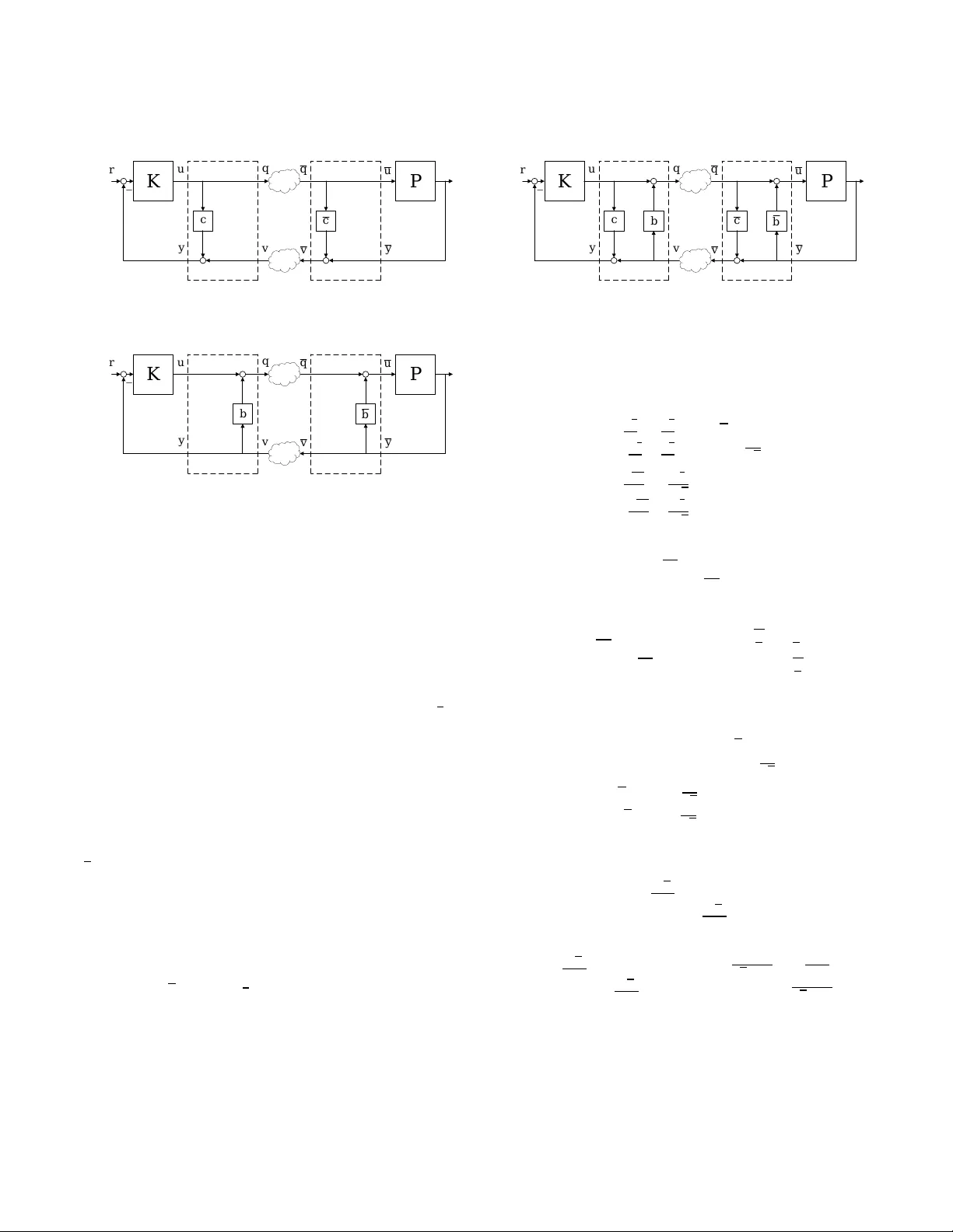
T wo- W ay Coding in Control Systems Under Injection Aacks: From Aack Detection to Aack Correction Song Fang School of Electrical Engineering and Computer Science, KTH Royal Institute of T echnology Stockholm, Sweden sonf@kth.se Karl Henrik Johansson School of Electrical Engineering and Computer Science, KTH Royal Institute of T echnology Stockholm, Sweden kallej@kth.se Mikael Skoglund School of Electrical Engineering and Computer Science, KTH Royal Institute of T echnology Stockholm, Sweden skoglund@kth.se Henrik Sandberg School of Electrical Engineering and Computer Science, KTH Royal Institute of T echnology Stockholm, Sweden hsan@kth.se Hideaki Ishii Department of Computer Science, T okyo Institute of T e chnology Y okohama, Japan ishii@c.titech.ac.jp ABSTRA CT In this paper , we introduce the method of two-way coding, a concept originating in communication theor y characteriz- ing coding schemes for two-way channels, into (networked) feedback control systems under injection attacks. W e rst show that the presence of two-way co ding can distort the perspective of the attacker on the control system. In general, the distorted viewpoint on the attacker side as a consequence of two-way coding will facilitate detecting the attacks, or restricting what the attacker can do, or e ven correcting the attack eect. In the particular case of zero-dynamics attacks, if the attacks are to be designe d according to the original plant, then they will be easily detected; while if the attacks are designed with respect to the equivalent plant as viewed by the attacker , then under the additional assumption that the plant is stabilizable by static output fe edback, the attack eect may be corrected in steady state. KEY W ORDS Cyber-physical system, networked control system, cyber- physical security , two-way channel, two-way coding, zero- dynamics attack 1 IN TRODUCTION The concept of two-way communication channels dates back to Shannon [ 26 ]. As its name indicates, in two-way channels, signals are transmitte d simultaneously in both directions between the two terminals of communication. Accordingly , coding for two-way channels should make use of the infor- mation contained in the data transmitte d in both directions; in other words, the coding schemes are also two-way , and thus are referred to as two-way coding [3, 5, 18]. Inherently , the communication channels in networked feedback control systems are two-way channels, with the controller side and the plant side being viewed as the two terminals of communication, respectively . Nevertheless, ap- proaches based on two-way coding for the two-way channels in networked feedback systems are rarely seen in the litera- ture. One exception is the so-called scattering transformation utilized in the tele-operation of robotics [ 2 , 10 , 11 , 13 , 21 , 22 ]; in a broad sense, scattering transformation can b e viewed as a special class of two-way coding to r esolve the issue of two-way time delays, the most essential characterization and the main issue of the two-way channels modeled on the input-output level in the problem of tele-operation. Other related applications of the scattering transformation include [9, 16, 17]. Particularly in the cyber-physical security problems (see, e.g., [ 1 , 4 , 8 , 15 , 20 , 23 – 25 , 27 , 29 , 32 ] and the references therein) of networked control systems, to the b est of our knowledge, only one-way coding has been employed. The authors of [ 31 ] introduced (one-way) encryption matrices into control systems to achieve condentiality and integrity . In [ 19 ], the authors considered a metho d of coding (using one-way co ding matrices) the sensor outputs in order to detect stealthy false data inje ction attacks in cyber-physical systems. Modulation matrices, which are one-way , were in- serted into cyber-physical systems in [ 12 ] to detect covert attacks and zero-dynamics attacks. Dynamic one-way cod- ing was applied to detect and isolate routing attacks [ 7 ] and replay attacks [ 6 ]. For remote state estimation in the pres- ence of eavesdr oppers, the so-called state-secrecy codes were introduced [ 30 ], which are also inherently one-way coding schemes. On the other hand, as will be discussed in Section 4 of this paper , one-way coding has its inherent limitations; for instance, one-way coding in general cannot eliminate the unstable p oles nor nonminimum-phase zeros of the plant nor the controller , which are most critical issues in the defense against, e.g., zero-dynamics attacks [29]. In this pap er , we investigate how two-way coding can play an important r ole in protecting the security of feedback control systems under injection attacks. W e rst introduce a series of special classes of two-way coding, including the two-way stretching, shearing, and rotation matrices, as well as the scattering transformation. W e then examine what changes the presence of two-way coding will bring to the feedback control system. On one hand, it is seen that on the controller and refer ence side, the plant behaves exactly as if two-way coding does not exist; as such, the controller may be designed regardless of two-way coding. On the other , two-way coding will distort the attacker’s perspective of the signals and systems, i.e., the components of the feedback loop, giving him/her a “transformed" view of the control system, and making the behaviors of the plant, controller , and reference all seemingly dier ent from the those of the original system without two-way coding. More specically , we examine ho w the presence of tw o- way co ding can play a critical role in the defense against injection attacks. In general, the distorted persp ective on the attacker side as a result of tw o-way coding will enable detecting the attacks or restricting what the attacker can do or even correcting the attack eect, dep ending on the attacker’s knowledge of the system. As a matter of fact, tw o- way coding can make the zeros and/or poles of the equivalent plant as viewed by the attacker all dierent from those of the original plant, and under some additional assumptions (i.e., the plant is stabilizable by static output feedback), the equivalent plant may even be made stable and/or minimum- phase. In the particular case of zero-dynamics attacks, it is then implicated that the attacks will b e detected if designed according to the original plant, while the attack eect may be corrected in steady state if the attacks are to be designed with respect to the equivalent plant. The remainder of the paper is organized as follo ws. Sec- tion 2 is devoted to two-way coding. In Section 3, we intro- duce two-way coding into linear time-invariant (LTI) feed- back control systems under injection attacks, and show how its presence can distort the perspective of the attacker . Sec- tion 4 analyzes the role tw o-way coding can play in the de- fense against injection attacks, in particular , zero-dynamics attacks. Concluding remarks are given in Section 5. 2 T W O- W A Y CODING Consider the single-input single-output (SISO) system de- picted in Fig. 1. Herein, K denotes the controller while P denotes the plant. The reference signal is r ( t ) ∈ R and the K P a d c b a d c b r y v u q q u y v − Figure 1: A networked feedback system with two-way coding. K P  1  − 1  −  r y v u q q u y v − Figure 2: A networked fe e dback system with one-way coding. plant output is y ( t ) ∈ R . In addition, let u ( t ) , u ( t ) , y ( t ) , q ( t ) , q ( t ) , v ( t ) , v ( t ) ∈ R . Denition 2.1. The (static) two-way co ding is dened as  q ( t ) y ( t )  = M  u ( t ) v ( t )  , (1) where M =  a b c d  . (2) Herein, a , b , c , d ∈ R are chosen such that ad , 0 , ad − bc , 0 . (3) Strictly speaking, it should b e further assumed that | ad − bc | < ∞ . Herein, two-way co ding (operating in a feedback loop) represents a tw o-way transformation that takes in the signal in the forward path and the signal in the fee dback path, and outputs a new signal to the forward path and a second new signal that passes on in the feedback path. In comparison, Fig. 2 depicts a system with one-way coding schemes, which are one-way transformations that either take in the signal in the forward path and output a new signal that passes on in the for ward path, or input the signal in the feedback path and output a signal that continues in the feedback path; herein, α , β ∈ R and 0 < | α | , | β | < ∞ . For simplicity , we denote the inverse of tw o-way coding M as  a b c d  = M − 1 =  d a d − b c − b a d − b c − c a d − b c a a d − b c  , (4) K P a d c b a d c b r y v u q q u y v − Figure 3: A fe edback system with two-way co ding. where a , b , c , d ∈ R . As illustrated on the plant side in Fig. 1, the inverse of two-way coding M denotes another two-way coding. At this point, we do not impose any assumptions on the controller K and plant P except that the closed-loop system is stable; we now prov e the following result for this generic setting. Proposition 2.2. If q ( t ) = q ( t ) and v ( t ) = v ( t ) , then u ( t ) = u ( t ) and y ( t ) = y ( t ) . Proof. Since  q ( t ) y ( t )  =  a b c d   u ( t ) v ( t )  , we have u ( t ) = a − 1 q ( t ) − a − 1 b v ( t ) , and y ( t ) = cu ( t ) + d v ( t ) = c a − 1 q ( t ) +  d − c a − 1 b  v ( t ) . Similarly , since  u ( t ) v ( t )  =  a b c d   q ( t ) y ( t )  , and noting (4), we have y ( t ) = − d − 1 cq ( t ) + d − 1 v ( t ) = c a − 1 q ( t ) +  d − c a − 1 b  v ( t ) , and u ( t ) = aq ( t ) + b y ( t ) =  a − bd − 1 c  q ( t ) + bd − 1 v ( t ) = a − 1 q ( t ) − a − 1 b v ( t ) . Clearly , when q ( t ) = q ( t ) and v ( t ) = v ( t ) , it follows that u ( t ) = u ( t ) and y ( t ) = y ( t ) . □ In other words, if q ( t ) = q ( t ) and v ( t ) = v ( t ) , the sys- tem in Fig. 1, now equivalent to that of Fig. 3, reduces to the system depicted in Fig. 4 as the “ original" feedback sys- tem without two-way coding. As such, properties, includ- ing stability and performance, of the system in Fig. 1 when q ( t ) = q ( t ) and v ( t ) = v ( t ) are equivalent to those of the original system in Fig. 4. K P r − yy = uu = Figure 4: The original fee dback system without two- way coding. K P a d a d r y v u q q u y v − Figure 5: A networked feedback system with two-way stretching matrix co ding. 2.1 Special Cases of T wo- W ay Coding W e now consider some sp ecial cases of two-way coding matrices. In what follows, we will introduce the (two-way ) stretching matrix, shearing matrix, r otation matrix, and so on that are adapted from 2D computer graphics [ 14 ], as well as the scattering transformation from tele-operation [2, 10, 11, 13, 21, 22]. 2.1.1 T wo- W ay Stretching Matrix. Below we list three cases of the two-way stretching matrices. Case 1: M =  a 0 0 1  , a , 0 . Case 2: M =  1 0 0 d  , d , 0 . Case 3: M =  a 0 0 d  , ad , 0 . In the case when ad = 1 , M is also known as the two-way squeezing matrix. The three cases of two-way str etching matrices are easy to understand; they are simply re-scalings of the signals. W e now only illustrate case 3 in Fig. 5. Herein, it is easy to see that a = 1 / a and d = 1 / d since M − 1 =  1 a 0 0 1 d  . As a matter of fact, the two-way stretching matrices re- duce to two one-way re-scaling transformations as one-way K P c c r y v u q q u y v − Figure 6: A networked feedback system with two-way shearing matrix coding: case 1. K P b b r y v u q q u y v − Figure 7: A networked feedback system with two-way shearing matrix coding: case 2. coding schemes (cf. Fig. 2); we will discuss the dierences b e- tween two-way coding and one-way coding in more details in the subsequent sections. 2.1.2 T wo- W ay Shearing Matrix. Three cases of the two-way shearing matrices are given below . Case 1: M =  1 0 c 1  , M − 1 =  1 0 − c 1  . In this case, we have the illustration given in Fig. 6, where c = − c . Simply speaking, the idea is to create a “parallel system" on the plant side, and compensate for it on the controller side. Case 2: M =  1 b 0 1  , M − 1 =  1 − b 0 1  . In this case, w e have the illustration giv en in Fig. 7, where b = − b . The idea is to add a “lo cal feedback controller" on the plant side, and compensate for it on the controller side. Case 3: M =  1 b c 1  , M − 1 =  1 − b − c 1  . Herein, bc , 1 . In this case, we have the illustration giv en in Fig. 8, where b = − b and c = − c . 2.1.3 T wo- W ay Rotation Matrix. The two-way rotation ma- trix and its inverse are given by M =  cos θ sin θ − sin θ cos θ  , M − 1 =  cos θ − sin θ sin θ cos θ  . K P c b c b r y v u q q u y v − Figure 8: A networked feedback system with two-way shearing matrix coding: case 3. Herein, θ , k π / 2 , k = 2 m + 1 , m ∈ Z . 2.1.4 Scaering Transformation. The scattering transforma- tion is given by [2, 10, 11, 13, 21, 22]  q ( t ) v ( t )  = " √ 2 2 √ 2 2 − √ 2 2 √ 2 2 #  √ γ 0 0 1 √ γ   u ( t ) y ( t )  =       √ 2 γ 2 √ 2 2 √ γ − √ 2 γ 2 √ 2 2 √ γ        u ( t ) y ( t )  . Herein, 0 < γ < ∞ . As a consequence,  q ( t ) y ( t )  =  √ 2 γ 1 γ √ 2 γ   u ( t ) v ( t )  . Correspondingly , M =  √ 2 γ 1 γ √ 2 γ  , M − 1 =       q 2 γ − 1 γ − 1 q 2 γ       . More generally , the scattering transformation can be ex- tended as [2, 10, 11, 13, 21, 22]  q ( t ) v ( t )  =  cos θ sin θ − sin θ cos θ   √ γ 0 0 1 √ γ   u ( t ) y ( t )  = " √ γ cos θ 1 √ γ sin θ − √ γ sin θ 1 √ γ cos θ #  u ( t ) y ( t )  . Herein, 0 < γ < ∞ and θ , k π / 2 , k = 2 m + 1 , m ∈ Z . As a result,  q ( t ) y ( t )  = " √ γ cos θ tan θ γ tan θ √ γ cos θ #  u ( t ) v ( t )  , and M = " √ γ cos θ tan θ γ tan θ √ γ cos θ # , M − 1 = " 1 √ γ cos θ − tan θ γ − tan θ 1 √ γ cos θ # . 3 ANAL YSIS OF LTI SYSTEMS WI TH T W O- W A Y CODING In this section, w e analyze in particular LTI feedback control systems. Consider the SISO feedback system with two-way K P a d c b a d c b r y v u q q u y v w z − Figure 9: A feedback system with two-way co ding un- der injection attacks. coding depicted in Fig. 9. Assume that herein the controller K and plant P are LTI with transfer functions K ( s ) and P ( s ) , respectively . In addition, let r ( t ) , u ( t ) , u ( t ) , y ( t ) , y ( t ) , q ( t ) , q ( t ) , v ( t ) , v ( t ) ∈ R . Meanwhile, suppose that injection (addi- tive) attacks w ( t ) ∈ R and z ( t ) ∈ R exist in the for ward path and feedback path of the control systems, respectively . Let R ( s ) , U ( s ) , U ( s ) , Y ( s ) , Y ( s ) , Q ( s ) , Q ( s ) , V ( s ) , V ( s ) , W ( s ) , Z ( s ) represent the Laplace transforms, assuming that they exist, of the signals r ( t ) , u ( t ) , u ( t ) , y ( t ) , y ( t ) , q ( t ) , q ( t ) , v ( t ) , v ( t ) , w ( t ) , z ( t ) . From now on, we assume that all the trans- fer functions of the systems are with zero initial conditions, unless otherwise spe cied. W e rst provide expressions for the Laplace transforms of the real plant output y ( t ) and the plant output y ( t ) as seen on the controller side, given refer ence r ( t ) and under injection attacks w ( t ) and z ( t ) . Theorem 3.1. Consider the SISO feedback system with two- way coding under injection attacks depicte d in Fig. 9. Assume that controller K and plant P are LTI with transfer functions K ( s ) and P ( s ) , respectively , and that the closed-loop system is stable. Then, Y ( s ) = K ( s ) P ( s ) 1 + K ( s ) P ( s ) R ( s ) + a − 1 [ 1 + c K ( s )] P ( s ) 1 + K ( s ) P ( s ) W ( s ) + a − 1 [ b − ( ad − bc ) K ( s )] P ( s ) 1 + K ( s ) P ( s ) Z ( s ) , (5) and Y ( s ) = K ( s ) P ( s ) 1 + K ( s ) P ( s ) R ( s ) + a − 1 [ P ( s ) − c ] 1 + K ( s ) P ( s ) W ( s ) + a − 1 [ ad − bc + b P ( s )] 1 + K ( s ) P ( s ) Z ( s ) . (6) Proof. Since Y ( s ) = P ( s ) U ( s ) , and U ( s ) = bY ( s ) + aQ ( s ) , we have U ( s ) = b P ( s ) U ( s ) + aQ ( s ) , and thus U ( s ) = aQ ( s ) 1 − b P ( s ) . Correspondingly , Y ( s ) = P ( s ) U ( s ) = aP ( s ) Q ( s ) 1 − b P ( s ) . As a consequence, V ( s ) = d Y ( s ) + c Q ( s ) = ad P ( s ) Q ( s ) 1 − b P ( s ) + c Q ( s ) = " ad P ( s ) 1 − b P ( s ) + c # Q ( s ) =  ad − bc  P ( s ) + c 1 − b P ( s ) Q ( s ) = P ( s ) − c ad − bc + b P ( s ) Q ( s ) . (7) Similarly , since U ( s ) = K ( s ) [ R ( s ) − Y ( s )] , and Y ( s ) = cU ( s ) + dV ( s ) , we have Y ( s ) = c K ( s ) [ R ( s ) − Y ( s )] + dV ( s ) , and hence Y ( s ) = c K ( s ) R ( s ) + dV ( s ) 1 + c K ( s ) . In addition, U ( s ) = K ( s ) [ R ( s ) − Y ( s )] = K ( s ) R ( s ) − K ( s ) [ c K ( s ) R ( s ) + dV ( s )] 1 + c K ( s ) = K ( s ) [ R ( s ) − dV ( s )] 1 + c K ( s ) . Thus, Q ( s ) = aU ( s ) + bV ( s ) = aK ( s ) 1 + c K ( s ) R ( s ) − ad K ( s ) 1 + c K ( s ) V ( s ) + bV ( s ) = aK ( s ) 1 + c K ( s ) R ( s ) + b − ( ad − bc ) K ( s ) 1 + c K ( s ) V ( s ) = b − ( ad − bc ) K ( s ) 1 + c K ( s )  aK ( s ) b − ( ad − bc ) K ( s )  R ( s ) + b − ( ad − bc ) K ( s ) 1 + c K ( s ) V ( s ) . (8) Using (7) and (8), while noting that Q ( s ) = Q ( s ) + W ( s ) , and V ( s ) = V ( s ) + Z ( s ) , we may then obtain that Q ( s ) = Q ( s ) + W ( s ) = W ( s ) + aK ( s ) 1 + c K ( s ) R ( s ) + b − ( ad − bc ) K ( s ) 1 + c K ( s ) V ( s ) = W ( s ) + aK ( s ) 1 + c K ( s ) R ( s ) + b − ( ad − bc ) K ( s ) 1 + c K ( s ) h V ( s ) + Z ( s ) i = W ( s ) + aK ( s ) 1 + c K ( s ) R ( s ) + b − ( ad − bc ) K ( s ) 1 + c K ( s )  P ( s ) − c ad − bc + b P ( s )  Q ( s ) + b − ( ad − bc ) K ( s ) 1 + c K ( s ) Z ( s ) . Hence,  1 − b − ( ad − bc ) K ( s ) 1 + c K ( s )  P ( s ) − c ad − bc + b P ( s )   Q ( s ) = W ( s ) + aK ( s ) 1 + c K ( s ) R ( s ) + b − ( ad − bc ) K ( s ) 1 + c K ( s ) Z ( s ) . On the other hand, 1 − b − ( ad − bc ) K ( s ) 1 + c K ( s )  P ( s ) − c ad − bc + b P ( s )  = [ 1 + c K ( s )] [ ad − bc + b P ( s )] [ 1 + c K ( s )] [ ad − bc + b P ( s )] − [ b − ( ad − bc ) K ( s )] [ P ( s ) − c ] [ 1 + c K ( s )] [ ad − bc + b P ( s )] = ad [ 1 + K ( s ) P ( s )] [ 1 + c K ( s )] [ ad − bc + b P ( s )] . As a result, Q ( s ) = d − 1 K ( s ) [ ad − bc + b P ( s )] 1 + K ( s ) P ( s ) R ( s ) + a − 1 d − 1 [ 1 + c K ( s )] [ ad − bc + b P ( s )] 1 + K ( s ) P ( s ) W ( s ) + a − 1 d − 1 [ b − ( ad − bc ) K ( s )] [ ad − bc + b P ( s )] 1 + K ( s ) P ( s ) Z ( s ) . Thus, Y ( s ) = aP ( s ) Q ( s ) 1 − b P ( s ) = d P ( s ) Q ( s ) ad − bc + b P ( s ) = K ( s ) P ( s ) 1 + K ( s ) P ( s ) R ( s ) + a − 1 [ 1 + c K ( s )] P ( s ) 1 + K ( s ) P ( s ) W ( s ) + a − 1 [ b − ( ad − bc ) K ( s )] P ( s ) 1 + K ( s ) P ( s ) Z ( s ) . Similarly , we have V ( s ) = V ( s ) + Z ( s ) = P ( s ) − c ad − bc + b P ( s ) Q ( s ) + Z ( s ) = P ( s ) − c ad − bc + b P ( s ) [ Q ( s ) + W ( s )] + Z ( s ) = P ( s ) − c ad − bc + b P ( s )  aK ( s ) 1 + c K ( s )  R ( s ) + P ( s ) − c ad − bc + b P ( s )  b − ( ad − bc ) K ( s ) 1 + c K ( s )  V ( s ) + P ( s ) − c ad − bc + b P ( s ) W ( s ) + Z ( s ) , and V ( s ) = d − 1 K ( s ) [ P ( s ) − c ] 1 + K ( s ) P ( s ) R ( s ) + a − 1 d − 1 [ 1 + c K ( s )] [ P ( s ) − c ] 1 + K ( s ) P ( s ) W ( s ) + a − 1 d − 1 [ 1 + c K ( s )] [ ad − bc + b P ( s )] 1 + K ( s ) P ( s ) Z ( s ) . Consequently , Y ( s ) = c K ( s ) R ( s ) + dV ( s ) 1 + c K ( s ) = K ( s ) P ( s ) 1 + K ( s ) P ( s ) R ( s ) + a − 1 [ P ( s ) − c ] 1 + K ( s ) P ( s ) W ( s ) + a − 1 [ ad − bc + b P ( s )] 1 + K ( s ) P ( s ) Z ( s ) . This completes the proof. □ Note that based on Theorem 3.1, Laplace transforms of all the signals owing in the feedback system can be obtained. For instance, since Y ( s ) = P ( s ) U ( s ) , it follows from (5) that plant input U ( s ) is given by U ( s ) = K ( s ) 1 + K ( s ) P ( s ) R ( s ) + a − 1 [ 1 + c K ( s )] 1 + K ( s ) P ( s ) W ( s ) + a − 1 [ b − ( ad − bc ) K ( s )] 1 + K ( s ) P ( s ) Z ( s ) . (9) W e now investigate the implications of The orem 3.1. It is clear that from the perspective of the reference, the transfer K P a d c b a d c b r y v u q q u y v w z − P K Figure 10: A feedback system with two-way co ding: from the viewpoint of the attacker . K P v q q v w z r Figure 11: A feedback system with two-way co ding: the equivalent system from the attacker’s viewpoint. K P y u u y w z r − Figure 12: The original fe edback system without two- way coding. function from reference R ( s ) to plant output Y ( s ) , found as K ( s ) P ( s ) 1 + K ( s ) P ( s ) , (10) stays exactly the same as in the original system depicted in Fig. 12 where two-way coding does not exist; therein, the transfer function from reference R ( s ) to plant output Y ( s ) is also given by (10) . As such, the controller K ( s ) may b e designed regardless of tw o-way coding. Meanwhile, to the attacker , the feedback system behaves dierently from the original system because of the presence of two-way coding, as will be shown in the following corollary . Corollary 3.2. From the viewpoint of the attacker (see Fig. 10), the fe e dback system is e quivalent to that of Fig. 11, where the transfer function of the equivalent plant P is given by P ( s ) = P ( s ) − c ad − bc + b P ( s ) , (11) while that of the equivalent controller K is found as K ( s ) = b − ( ad − bc ) K ( s ) 1 + c K ( s ) . (12) In addition, the Laplace transform of the e quivalent reference signal r is R ( s ) = aK ( s ) b − ( ad − bc ) K ( s ) R ( s ) . (13) Proof. Equations (11) , (12) , and (13) follow directly from (7) and (8). □ Clearly , the presence of two-way coding will distort the attacker’s view of the control system, making the properties of the plant, controller , and reference all seemingly dierent from those of the original system. This distorted perspective will assist in defending the system against attacks that ar e designed based on the system models, as will be seen shortly in the next section. 4 A T T A CK DETECTION AND CORRECTION In this section, we examine how the presence of two-way coding can play a critical role in the defense against injection attacks in LTI systems. In general, the distorted perspe ctive on the attacker side as a result of two-way coding will enable detecting the attacks or restricting what the attacker can do or even correcting the attack eect, dep ending on the attacker’s knowledge of the system. In the particular case of zero-dynamics attacks, it is seen that the attacks will be detected if designed according to the original plant, while the attack eect will be corrected in steady state if the attacks are to be designed with respect to the equivalent plant as seen by the attacker . Before we procee d, we rst prov e the following result. Consider still the SISO fe edback system depicte d in Fig. 9. Without physically changing P ( s ) , we can use two-way cod- ing to make the zeros and/or poles of the equivalent plant P ( s ) , as seen by the attacker , all dierent from those of the original plant P ( s ) . Theorem 4.1. Let P ( s ) = m P ( s ) n P ( s ) , (14) where m P ( s ) and n P ( s ) denote the numerator and denominator polynomials of P ( s ) , respectively . Suppose that m P ( s ) and n P ( s ) are coprime. • The zeros of P ( s ) are given by the roots of m P ( s ) − c n P ( s ) = 0 . (15) In addition, if c , 0 , then the zeros of P ( s ) are all dier- ent from those of P ( s ) . • The poles of P ( s ) are given by the roots of ( ad − bc ) n P ( s ) + bm P ( s ) = 0 . (16) In addition, if b , 0 , then the poles of P ( s ) are all dier- ent from those of P ( s ) . Proof. It is clear that P ( s ) = P ( s ) − c ad − bc + b P ( s ) = m P ( s ) − c n P ( s ) ( ad − bc ) n P ( s ) + bm P ( s ) . Note that the zeros of P ( s ) are given by the roots of m P ( s ) = 0 . Let z i be a zero of P ( s ) . Hence, m P ( z i ) = 0 . Then, z i cannot be a zero of P ( s ) , otherwise this will lead to n P ( z i ) = m P ( z i ) / c = 0 and thus z i will be a pole of P ( s ) , which contradicts the fact that m P ( s ) and n P ( s ) are coprime . Similarly , note that the poles of P ( s ) are given by the roots of n P ( s ) = 0 . Let p i be a pole of P ( s ) . Therefore, n P ( p i ) = 0 . Then, p i cannot be a p ole of P ( s ) , otherwise this will lead to m P ( p i ) = ( ad − bc ) n P ( p i ) / b = 0 and thus p i will be a zero of P ( s ) , which contradicts the fact that m P ( s ) and n P ( s ) are coprime. □ Note that herein the conditions c , 0 and/or b , 0 are essential. Similarly to Theorem 4.1, it can also be sho wn that the zeros of K ( s ) are all dierent from those of K ( s ) when b , 0 , while the poles of K ( s ) are all dierent from those of K ( s ) when c , 0 . W e now remark on some fundamental dierences between two-way coding and one-way coding. It is clear that two- way coding reduces to two one-way coding schemes when b = c = 0 (as in the case of two-way str etching matrix; see Section 2.1.1), and correspondingly , P ( s ) = P ( s ) ad , K ( s ) = ad K ( s ) . (17) It is clear that the zeros and p oles of P ( s ) and K ( s ) are ex- actly the same as those of P ( s ) and K ( s ) . In other words, one- way coding will not change the zeros nor poles of the plant nor the controller . Indeed, similar results hold for multiple- input multiple-output (MIMO) systems as well. It is also worth mentioning that even with dynamic one-way coding schemes, since cancellations b etween unstable poles and nonminimum-phase zeros should always be avoided to pre- vent possible internal instability , the nonminimum-phase zeros and unstable poles of the original plant and controller cannot be eliminated. W e next show that the presence of two-way co ding not only can make the zeros and/or poles of the equivalent plant P ( s ) all dierent from those of the original plant P ( s ) , but also, under some additional conditions, may render P ( s ) stable and/or minimum-phase. In fact, similar results hold for the pair of the e quivalent controller K ( s ) and the original controller K ( s ) as well. Theorem 4.2. Suppose that a minimal realization of the plant P ( s ) is given by  Û x ( t ) = Ax ( t ) + Bu ( t ) , y ( t ) = C x ( t ) + Du ( t ) . (18) If the plant is stabilizable by static output feedback [ 28 ] de- scribed as u ( t ) = F y ( t ) , (19) where F ∈ R , then all the poles of P ( s ) can be made stable, while all the zeros of P ( s ) can be made minimum-phase. Proof. Since (18) is a minimal realization of P ( s ) , we have P ( s ) = m P ( s ) n P ( s ) = C ( s I − A ) − 1 B + D . Meanwhile, since P is stabilizable by static output feedback, there exists a non-zero constant F 1 such that 1 1 + F 1  C ( s I − A ) − 1 B + D  = 1 1 + F 1 h m P ( s ) n P ( s ) i = n P ( s ) n P ( s ) + F 1 m P ( s ) is stable, i.e., all its poles are stable. In other words, all the roots of n P ( s ) + F 1 m P ( s ) are with negative r eal parts. Mean- while, note that P ( s ) = P ( s ) − c ad − bc + b P ( s ) = m P ( s ) − c n P ( s ) ( ad − bc ) n P ( s ) + bm P ( s ) . As such, when b / ( ad − bc ) = F 1 , ( ad − bc ) n P ( s ) + bm P ( s ) = ( ad − bc ) [ n P ( s ) + F 1 m P ( s )] , and hence all its roots are with negative r eal parts, i.e., all the poles of P ( s ) are stable. Similarly , when c = − 1 / F 2 , where F 2 is a stabilizing, non-zero static output feedback control gain, we have m P ( s ) − c n P ( s ) = − c [ n P ( s ) + F 2 m P ( s )] , and thus all its roots are with negative real parts, i.e., all the zeros of P ( s ) are minimum-phase. □ From the proof, it can be seen that it is possible to make all the poles of P ( s ) stable and all the zer os of P ( s ) minimum- phase simultaneously , as long as F 1 , F 2 . It is also worth mentioning that herein we only require the plant to be stabilizable by static output feedback F , which is used merely for the purpose of deciding the parameters of two-way coding, but the controller K ( s ) is not necessarily chosen among such static controllers; stated alternatively , the controller K ( s ) are not further restricted. 4.1 Zero-Dynamics Attacks W e next examine the implications of Theorem 4.1 and The- orem 4.2 in the attack detection and correction of zero- dynamics attacks [ 29 ]. Consider rst the original system in Fig. 12. For zero-dynamics attacks, the typical attack design is to let Z ( s ) = 0 and W ( s ) = w 0 s − ζ , (20) where ζ is a zero of P ( s ) . It is known that if w 0 is chosen correspondingly , then the attack cannot b e dete cted, as a consequence of the blocking property of zeros. Consider next the system with tw o-way coding in Fig. 9 where the equivalent plant from the perspective of the at- tacker is given by P ( s ) . If the zero-dynamics attacks are still designed in terms of the zeros of P ( s ) , then they will easily be dete cted as long as c , 0 , since the zeros of P ( s ) are all dierent from those of P ( s ) . On the other hand, if the attacker somehow knows P ( s ) (e .g., by carrying out system identication based on q ( t ) and v ( t ) , or by knowing a , b , c , d as w ell as P ( s ) ) and designs the zero-dynamics attacks accordingly , then the attacks cannot be detected. In this case, note that if the plant P is stabilizable by static output feedback, then all the zer os of P ( s ) can be made minimum-phase. As a result, only stable zero-dynamics attacks are possible, meaning that the attack signal and hence the attack response will be zero in steady state; in such a case, we say that the attack eect can be corrected. W e summarize the ab ove discussions in the following corollary . Corollary 4.3. Consider the system with two-way coding in Fig. 9 under zero-dynamics attack given by (20) . • If the zero-dynamics attack is designed according to P ( s ) , then it can always be detected with c , 0 . • If the zero-dynamics attack is designed with respect to P ( s ) , then, supposing that the plant P is stabilizable by static output fe e dback, all the zeros of P ( s ) can b e made minimum-phase, in which case the attack eect will b e corrected in steady state. Note also that for zero-dynamics attacks, the attacker may instead choose to let W ( s ) = 0 and Z ( s ) = z 0 s − λ , (21) where λ is a pole of P ( s ) (and hence a zero of the close d- loop system from z ( t ) to plant output y ( t ) ). If z 0 is chosen correspondingly , then the attack cannot be detected. Sim- ilarly , in the system with two-way co ding in Fig. 9, if the zero-dynamics attacks are still designed in terms of the poles of P ( s ) , they will easily b e detected as long as b , 0 , since the poles of P ( s ) are all dierent from those of P ( s ) . On the other hand, if the attacker knows P ( s ) and designs the zero- dynamics attacks accordingly , then the attacks cannot be detected. In this case, note that if the plant P is stabilizable by static output feedback, then all the poles of P ( s ) can be made stable. As a consequence, only stable zero-dynamics attacks are possible, meaning that the attack eect will be zero in steady state; in such a situation, the attack eect is said to be corrected. Similarly , we summarize the pre vious discussions in the corollary below . Corollary 4.4. Consider the system with two-way coding in Fig. 9 under zero-dynamics attack given by (21) . • If the zero-dynamics attack is designed according to P ( s ) , then it can always be detected with b , 0 . • If the zero-dynamics attack is designed with respect to P ( s ) , then, supposing that the plant P is stabilizable by static output fe edback, all the poles of P ( s ) can be made stable, in which case the attack eect will be correcte d in steady state. When the zero-dynamics attacks (20) and (21) happen simultaneously , it is clear that Corollary 4.3 and Corollary 4.4 apply respectively to the two attacks. It might also be interesting to examine what changes two- way co ding can bring to the detection and correction of other classes of injection attacks; see, e.g., [ 23 ]. W e will, however , leave those investigations to future r esearch. 5 CONCLUSIONS W e hav e introduced the method of two-way co ding into feed- back control systems under injection attacks. W e have shown that the presence of two-way coding can distort the perspec- tive of the attacker on the control system; this distorted view on the attacker side was demonstrated to facilitate detecting the attacks, or restricting what the attacker can do, or e ven correcting the attack eect in steady state. Future research di- rections include the analysis of MIMO systems, discrete-time systems, as well as other classes of attacks in the presence of two-way coding. A CKNO WLEDGMEN TS The work is supp orted by the Knut and Alice W allenberg Foundation, the Swedish Strategic Research Foundation, the Swedish Research Council, the Swedish Civil Contingencies Agency (CERCES project), the JSPS under Grant-in- Aid for Scientic Research Grant No.: 15H04020, and the JST CREST under Grant No.: JPMJCR15K3. REFERENCES [1] Saurabh Amin, Galina A. Schwartz, Alvaro A. Cárdenas, and S. Shankar Sastry . 2015. Game-theoretic models of electricity theft detection in smart utility networks: Providing new capabilities with advanced metering infrastructure. IEEE Control Systems Magazine 35, 1 (2015), 66–81. [2] Robert J. Anderson and Mark W . Spong. 1989. Bilateral control of teleoperators with time delay . IEEE Trans. A utomat. Control 34, 5 (1989), 494–501. [3] Anas Chaaban and A ydin Sezgin. 2015. Multi-way communications: An information theoretic perspective. Foundations and Trends ® in Communications and Information The or y 12, 3-4 (2015), 185–371. [4] Peng Cheng, Ling Shi, and Bruno Sinopoli. 2017. Guest editorial special issue on secure control of cyber-physical systems. IEEE Transactions on Control of Network Systems 4, 1 (2017), 1–3. [5] Edward C. V an der Meulen. 1977. A survey of multi-way channels in information theor y: 1961-1976. IEEE Transactions on Information Theory 23, 1 (1977), 1–37. [6] Riccardo M.G. Ferrari and André M.H. T eixeira. 2017. Detection and isolation of replay attacks through sensor watermarking. IF AC- PapersOnLine 50, 1 (2017), 7363–7368. [7] Riccardo M.G. Ferrari and André M.H. T eixeira. 2017. Detection and isolation of routing attacks through sensor watermarking. In Proceed- ings of the American Control Conference . 5436–5442. [8] Jairo Giraldo, David Urbina, Alvaro Car denas, Junia V alente, Mustafa Faisal, Justin Ruths, Nils Ole Tippenhauer , Henrik Sandb erg, and Richard Candell. 2018. A Survey of Physics-Based Attack Detection in Cyber-Physical Systems. ACM Computing Surveys (CSUR) 51, 4 (2018), 76. [9] Guoxiang Gu and Li Qiu. 2011. A two-port approach to networked feedback stabilization. In Proceedings of the IEEE Conference on Decision and Control and European Control Conference . 2387–2392. [10] T akeshi Hatanaka, Nikhil Chopra, Masayuki Fujita, and Mark W . Spong. 2015. Passivity-based control and estimation in networked robotics . Springer . [11] Sandra Hirche and Martin Buss. 2012. Human-oriented control for haptic teleoperation. Proc. IEEE (2012). [12] Andreas Hoehn and Ping Zhang. 2016. Detection of covert attacks and zero dynamics attacks in cyber-physical systems. In Proceedings of the A merican Control Conference . 302–307. [13] Peter F. Hokay em and Mark W . Spong. 2006. Bilateral teleoperation: An historical survey . A utomatica 42, 12 (2006), 2035–2057. [14] John F Hughes, Andries V an Dam, James D. Foley , Morgan McGuire, Steven K. Feiner , David F. Sklar , and Kurt Akeley . 2014. Computer Graphics: Principles and Practice . Pearson. [15] Karl H. Johansson, George J. Pappas, Paulo T abuada, and Claire J. T omlin. 2014. Guest editorial special issue on control of cyber-physical systems. IEEE Trans. A utomat. Control 59, 12 (2014), 3120–3121. [16] Thomas Kailath, Ali H. Sayed, and Babak Hassibi. 2000. Linear Estima- tion . Prentice Hall. [17] Hidenori Kimura. 1996. Chain-scattering approach to H ∞ control . Springer . [18] Hendrik B. Meeuwissen. 1998. Information the oretical aspects of two- way communication . T echnische Universiteit Eindhoven. [19] Fei Miao, Quanyan Zhu, Miroslav Pajic, and George J. Pappas. 2017. Coding schemes for securing cyb er-physical systems against stealthy data injection attacks. IEEE Transactions on Control of Network Systems 4, 1 (2017), 106–117. [20] Yilin Mo, Sean W eerakkody, and Bruno Sinopoli. 2015. Physical au- thentication of control systems: Designing watermarked control inputs to detect counterfeit sensor outputs. IEEE Control Systems Magazine 35, 1 (2015), 93–109. [21] Günter Niemeyer and Jean-Jacques E. Slotine. 1991. Stable adaptive teleoperation. IEEE Journal of Oceanic Engineering 16, 1 (1991), 152– 162. [22] Emmanuel Nuño, Luis Basañez, and Romeo Ortega. 2011. Passivity- based control for bilateral teleoperation: A tutorial. Automatica 47, 3 (2011), 485–495. [23] Fabio Pasqualetti, Florian Dorer , and Francesco Bullo. 2015. Control- theoretic metho ds for cyb erphysical se curity: Ge ometric principles for optimal cross-layer resilient control systems. IEEE Control Systems Magazine 35, 1 (2015), 110–127. [24] Radha Poovendran, Krishna Sampigethaya, Sandeep Kumar S. Gupta, Insup Lee , K. V enkatesh Prasad, David Corman, and James L. Paunicka. 2012. Special issue on cyb er-physical systems [scanning the issue]. Proc. IEEE 100, 1 (2012), 6–12. [25] Henrik Sandberg, Saurabh Amin, and Karl H. Johansson. 2015. Cyb er- physical security in networked control systems: An introduction to the issue. IEEE Control Systems Magazine 35, 1 (2015), 20–23. [26] Claude E. Shannon. 1961. T wo-way communication channels. In Pro- ceedings of the Fourth Berkeley Symposium on Mathematical Statistics and Probability . [27] Roy S. Smith. 2015. Covert misappropriation of networked control sys- tems: Presenting a feedback structure. IEEE Control Systems Magazine 35, 1 (2015), 82–92. [28] V assilis L. Syrmos, Chaouki T . Abdallah, Peter Dorato, and Karolos Grigoriadis. 1997. Static output feedback: A sur vey . Automatica 33, 2 (1997), 125–137. [29] Andre T eixeira, Kin C. Sou, Henrik Sandberg, and Karl H. Johans- son. 2015. Secure control systems: A quantitative risk management approach. IEEE Control Systems Magazine 35, 1 (2015), 24–45. [30] Anastasios T siamis, Konstantinos Gatsis, and George J. Pappas. 2017. State estimation codes for perfect secrecy . In Proceedings of the IEEE Conference on Decision and Control . 176–181. [31] Zhiheng Xu and Quanyan Zhu. 2015. Secure and resilient control design for cloud enabled networked control systems. In Proceedings of the First ACM W orkshop on Cyb er-Physical Systems-Security and/or PrivaCy . 31–42. [32] Quanyan Zhu and Tamer Basar . 2015. Game-theoretic methods for robustness, security , and resilience of cyberphysical control systems: Games-in-games principle for optimal cross-layer resilient control systems. IEEE Control Systems Magazine 35, 1 (2015), 46–65.