To Retransmit or Not: Real-Time Remote Estimation in Wireless Networked Control

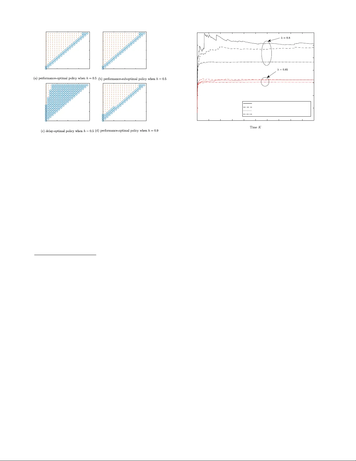
T o Retransmit or Not: Real-T ime Remote Estimation in W ireless Netw orked Control Kang Huang, W anchun Liu † , Y onghui Li, and Branka V ucetic School of Electrical and Information Engineering, The Uni versity of Sydney , Australia Emails: { kang.huang, wanchun.liu, yonghui.li, branka.vucetic } @sydne y .edu.au. Abstract — Real-time remote estimation is critical f or mission- critical applications including industrial automation, smart grid, and the tactile Internet. In this paper , we propose a hybrid automatic repeat request (HARQ)-based real-time r emote estima- tion framework for linear time-in variant (L TI) dynamic systems. Considering the estimation quality of such a system, there is a fundamental tradeoff between the reliability and freshness of the sensor’s measurement transmission. When a failed trans- mission occurs, the sensor can either retransmit the pr evious old measurement such that the r eceiver can obtain a mor e reliable old measurement, or transmit a new but less reliable measurement. T o design the optimal decision, we formulate a new problem to optimize the sensor’s online decision policy , i.e., to retransmit or not, depending on both the current estimation quality of the remote estimator and the curr ent number of retransmissions of the sensor , so as to minimize the long-term remote estimation mean-squared error (MSE). This problem is non-trivial. In particular , it is not clear what the condition is in terms of the communication channel quality and the L TI system parameters, to ensure that the long-term estimation MSE can be bounded. W e give a sufficient condition of the existence of a stationary and deterministic optimal policy that stabilizes the r emote estimation system and minimizes the MSE. Also, we pro ve that the optimal policy has a switching structure, and derive a low-complexity suboptimal policy . Our numerical results show that the proposed optimal policy notably improves the performance of the remote estimation system compared to the con ventional non-HARQ policy . I . I N T RO D U C T I O N Real-time remote estimation is critical for netw orked control applications such as industrial automation, smart grid, vehicle platooning, drone swarming, immersive virtual reality (VR) and the tactile Internet [1]. For such real-time applications, high-quality remote estimation of the states of dynamic pro- cesses ov er unreliable links is a major challenge. The sensor’ s sampling policy , the estimation scheme at a remote receiver , and the communication protocol for state-information delivery between the sensor and the receiver should be designed jointly . T o enable optimal design of wireless remote estimation, the performance metric for the remote estimation system needs to be selected properly . F or some applications, the model of the dynamic process under monitoring is unkno wn and the recei ver is not able to estimate the current state of the process based on the previously receiv ed states, i.e., a state- monitoring-only scenario [2]. In this scenario, the performance metric is the age-of-information (AoI), which reflects ho w old the freshest received sensor measurement is, since the † W . Liu is the corresponding author . moment that measurement was generated at the sensor [2]. Howe v er , in practice, most of the dynamic processes are time- correlated, and the state-changing rules can be known by the receiv er to some extent. Therefore, the receiver can estimate the current state of the process based on the previously receiv ed measurements and the model of the dynamic process (see e.g., [3], [4]), especially when the packet that carries the current sensor measurement is failed or delayed. In this sense, the estimation mean-squared error (MSE) is the perfect performance metric. From a communication protocol design perspectiv e, we naturally ask: does a sensor need retransmission or not for mission-critical real-time remote estimation? Retransmission is required by con ventional communication systems with non- real-time backlogged data to be perfectly delivered to the receiv ers. Also, ener gy-constrained remote estimation systems and the ones with lo w sampling rate can also benefit from retransmissions, see e.g., [5] and [6]. It seems that retrans- missions may not impro ve the performance of a mission- critical real-time remote estimation system [7], which is not mainly constrained by energy nor sampling rate, as it is a waste of transmission opportunity to transmit an out-of-date measurement instead of the current one. Howe ver , this is true only when a retransmission has the same success probability as a ne w transmission, e.g., with the standard automatic repeat request (ARQ) protocol. Note that a hybrid ARQ (HARQ) pro- tocol, e.g., with a chase combining or incremental redundancy scheme, is able to effecti vely increase the successful detection probability of a retransmission by combining multiple copies from previously failed transmissions [8]. Therefore, a HARQ protocol has the potential to impro ve the performance of real-time remote estimation. Howe ver , to the best of our knowledge, HARQ has never been considered in the open literature of real-time remote estimation of a time-correlated dynamic process. In the paper, we introduce HARQ into real-time remote estimation systems and optimally design the sensor’ s trans- mission policy to minimize the estimation MSE. Note that there is a fundamental tradeoff between the reliability and freshness of the sensor’ s measurement transmission. When a failed transmission occurs, the sensor can either retransmit the previous old measurement such that the recei ver can obtain a more reliable old measurement, or transmit a new but less reliable measurement. The main contributions of the paper are summarized as follows: • W e propose a novel HARQ-based real-time remote esti- mation system, where the sensor makes online decision to send a new measurement or retransmit the previously failed one depending on both the current estimation quality of the receiver and the current number of retrans- missions of the sensor . • W e formulate the problem to optimize the sensor’ s deci- sion policy so as to maximize the long-term performance of the receiv er in terms of the average MSE. Since it is not clear whether the long-term a verage MSE can be bounded or not, we gi ve a sufficient condition in terms of the communication channel quality and the L TI system parameters to ensure that an optimal policy exists and stabilizes the remote estimation system. • W e deriv e a structural property of the optimal policy , i.e., the optimal polic y is a switching-type policy , and giv e an easy-to-compute suboptimal policy . Our numerical results show that the suboptimal policy can efficiently improv e the system performance than the con ventional non-HARQ policy , under the setting of practical system parameters. I I . S Y S T E M M O D E L W e consider a basic system setting that a smart sensor peri- odically samples, pre-estimates and sends its local estimation of a dynamic process to a remote recei ver through a wireless link with packet dropouts, as illustrated in Fig. 1. A. Dynamic Pr ocess Modeling W e consider a general discrete linear time-in variant (L TI) model for the dynamic process as (see e.g., [9]–[11]) x k +1 = Ax k + w k , y k = C x k + v k , (1) where the discrete time steps are determined by the sensors sampling period T s , x k ∈ R n is the process state vector , A ∈ R n × n is the state transition matrix, y k ∈ R m is the measurement vector of the smart sensor attached to the process, C ∈ R m × n is the measurement matrix 2 , w k ∈ R n and v k ∈ R m are the process and measurement noise vectors, respectiv ely . W e assume w k and v k are independent and are identically distributed (i.i.d.) zero-mean Gaussian processes with corresponding cov ariance matrices Q and R , respecti vely . The initial state x 0 is zero-mean Gaussian with cov ariance ma- trix Σ 0 . T o av oid tri vial problems, we assume that ρ 2 ( A ) > 1 , where ρ 2 ( A ) is the maximum squared eigenv alue of A [13]. B. State Estimation at the Smart Sensor Since the sensor’ s measurements are noisy , the smart sensor with suf ficient computation and storage capacity is required to estimate the state of the process, x k , using a Kalman filter [10], 2 Note that C is not necessary to be full rank [12], as illustrated in Fig. 1, i.e., x k is a two-dimensional (2D) signal, while the measurement y k is one- dimensional. After Kalman filtering, we have a 2D ˆ x s k . Process Sampler Kalman Filter Tx Blo c k (H)ARQ Remote Estimator Pac k et-Drop Channel (H)ARQ F eedback ˆ x k x k y k ˆ x s k a k time, k x k, 1 x k, 2 time, k y k time, k ˆ x s k, 1 ˆ x s k, 2 δ k Fig. 1. Proposed remote estimation system with HARQ, where x k ,  x k, 1 , x k, 2  T is the two-dimensional state vector of the dynamic process. [11], which gi ves the minimum estimation MSE, based on the current and previous raw measurements: x s k | k − 1 = Ax s k − 1 | k − 1 (2a) P s k | k − 1 = AP s k − 1 | k − 1 A T + Q (2b) K k = P s k | k − 1 C T ( C P s k | k − 1 C T + R ) − 1 (2c) x s k | k = x s k | k − 1 + K k ( y k − C x s k | k − 1 ) (2d) P s k | k = ( I − K k C ) P s k | k − 1 (2e) where I is the m × m identity matrix, ( · ) T is the transpose operator , x s k | k − 1 is the priori state estimation, x s k | k is the posteriori state estimation at time k , K k is the Kalman gain, P k | k − 1 and P k | k represent the priori and posterior error cov ariance at time k , respecti vely . The first two equations present the prediction steps while the last three equations present the updating steps [12]. Note that x s k | k is the output of the Kalman filter at time k , i.e., the pre-filtered measurement of y k , with the estimation error covariance P s k | k . As we focus on the effect of communication protocols on the stability and quality of the remote estimation, we assume that the local estimation is stable as follows [10], [11]. Assumption 1. The local Kalman filter of system (1) is stable with the system parameters { A, C, Q } 3 , i.e., the error cov ariance matrix P s k | k con ver ges to a finite matrix ¯ P 0 when k is sufficiently large. In the r est of the paper , we assume that the local Kalman filter operates in the steady state [10], [11], i.e., P s k | k = ¯ P 0 . F or ease of notation, we use ˆ x s k to denote the sensor’ s estimation, x s k | k . C. Communication and Remote Estimation The sensor transmits its pre-filtered measurement in a packet and sends it to the receiver (i.e., the remote estima- tor) through a static channel, which is modeled as an i.i.d. packet-dropping process. 4 Let (1 − λ ) denotes the packet- drop probability . Note that the successful pack et detection pr obability at the receiv er can be different for different trans- mission/retransmission schemes. 3 The rigorous stability condition in terms of { A, C , Q } is given in [12]. 4 General fading and Markov channels can be considered in our future work. W e assume that the packet length is equal to the sampling period T s . Thus, there e xists a unit transmission delay between the sensor and the r eceiver . For e xample, the sensor’ s raw measurement at the beginning of time slot k is filtered and sent to the receiver before time slot ( k + 1) . Also, we assume that the acknowledgement/ne gati ve-ackno wledgement (A CK/N A CK) message is fed back from the receiv er to the sensor perfectly without any delay , when the packet detection succeeds/fails. If an A CK is receiv ed by the sensor, it will send a ne w (pre-filtered) measurement in the next time slot. If a NA CK is recei ved, the sensor may decide whether to retransmit the unsuccessfully transmitted measurement based on its ARQ protocol or to send the new measurement. In the rest of this section, we introduce the standard ARQ-based estimation system. The proposed HARQ-based protocol will be presented in Sec. III. Standar d ARQ-Based Remote Estimation. For the standard ARQ protocol, the recei ver discards the failed packets, and the sensor simply resends the previously failed packet if a re- transmission is required. Thus, the successful packet detection probability at each time is independent of the current number of retransmissions. Let the random v ariable δ ARQ k ∈ { 0 , 1 } denote the failed/successful packet detection at the receiver in time slot k . W e hav e P h δ ARQ k = 1 i = λ, ∀ k . (3) As the chances of the successful detection of a new transmis- sion and a retransmission are the same, the optimal policy is to always transmit the current sensor estimation, i.e., a non- r etransmission policy [7]. Consider the non-retransmission policy . As the successfully detected packet contains the estimated state information with a one-step delay , the receiver needs to estimate the current state based on the dynamic process model (1). If the pack et detection is failed, the receiv er can estimate the current state based on its previous estimation and the process model. Therefore, the optimal estimator at the receiv er is giv en as [3] ˆ x k = ( A ˆ x s k − 1 , if δ ARQ k − 1 = 1 A ˆ x k − 1 , otherwise. (4) I I I . H A R Q - B A S E D R E M O TE E S T I M A T I O N For a HARQ protocol, the recei v er b uf fers the incorrectly receiv ed packets, and the detection of the retransmitted packet depends on all the buffered related packets. 5 Thus, the prob- ability of successful packet detection in time slot k , depends on the number of consecutiv e retransmissions r k ≥ 0 [15]. In particular , r k = 0 indicates a new transmission in time slot k . Let the random variable δ HARQ k ∈ { 0 , 1 } denote the failed/successful packet detection at the recei ver in time slot k . 5 T o be specific, if a retransmission is required, the sensor can either resend the previously failed packet (i.e., a chase combining scheme) or send a retransmission packet that contains different information than the previous one (i.e., a incremental redundancy scheme). The recei ver is possible to successfully detect the current retransmission packet based on the previously erroneously received ones [14], [15]. X × × X × X × × × × Time slots · · · · · · k − 3 k Fig. 2. An illustration of the sensor’s transmission process. The solid circles denote the raw measurement sampling time, the up arrows are the starting points of ne w transmissions (i.e., only these (pre-filtered) measurements will be sent to the receiver), solid/dashed blocks are new/re-transmission packets, and X / × denotes a successful/failed detection at the receiv er . Thus, the successful packet detection probability is given as [15] P h δ HARQ k = 1 i = 1 − g ( r k ) , ∀ k , (5) where the function g ( · ) is determined by the specific HARQ protocol (e.g., with chase combining or incremental redun- dancy). Specifically , 1 − g (0) = λ and g (0) > g ( r ) when r > 0 , i.e., a retr ansmission is more r eliable than a ne w transmission. In this scenario, when a failed transmission occurs, there exists an inherent trade-off between retransmitting previously failed local state estimation with a higher success probability , and sending the current state estimation with a lower success probability . Therefore, the sensor needs to properly decide when to transmit a new estimation and when to retransmit. Let a k ∈ { 0 , 1 } be the sensor’ s decision variable at time k , as illustrated in Fig. 1. If a k = 0 , the sensor sends the new measurement to the receiv er in time slot k ; otherwise, it retransmits the unsuccessfully transmitted measurement. Thus, the current number of retransmissions, r k , has the update rule as r k = ( 0 , if a k = 0 r k − 1 + 1 , otherwise. (6) If a packet transmitted in time slot ( k − 1) is successfully detected, the receiver can estimate the current state x k based on the recei ved sensor’ s estimation at ( k − 1 − r k − 1 ) as illustrated in Fig. 2, and the system dynamics (1). Otherwise, the receiver can only do estimation based on the previous one. Thus, the receiver estimator based on HARQ is giv en as ˆ x k =      A ˆ x s k − 1 , if a k − 1 = 0 and δ HARQ k − 1 = 1 A r k − 1 +1 ˆ x s k − r k − 1 − 1 , if a k − 1 = 1 and δ HARQ k − 1 = 1 A ˆ x k − 1 , otherwise. (7) From the second expression of (7), the estimation quality of x k is not good if r k − 1 is large, since the recei ver’ s current estimation ˆ x k is based on the sensor’ s measurement at time ( k − r k − 1 − 1) , i.e., an out-of-date information. From the last expression of (7), the estimation quality of x k is bad if there is a sequence of failed transmissions and the receiv er estimates the current state based on the one sent by the sensor a long time ago. For ease of analysis, we define the estimation quality inde x, q k , as q k , k − t k , (8) where t k is the generation time slot of the latest sensor’ s estimation that is successfully receiv ed by the receiv er before time slot ( k + 1) , 6 and q k ≥ 0 . As it is straightforward that t k = ( k − r k , if δ HARQ k = 1 t k − 1 , otherwise , we have q k = ( r k , if δ HARQ k = 1 q k − 1 + 1 , otherwise. (9) Therefore, the last iteration expression in (7) can be further written as ˆ x k = A q k − 1 +1 ˆ x s k − q k − 1 − 1 , if δ HARQ k − 1 = 0 . (10) In other words, the recei ver estimation at time k is based on the state estimation of the smart sensor at time ( k − q k − 1 − 1) . Therefore, from (7), (9) and (10), the estimation error cov ariance can be obtained as P k , E  ( x k − ˆ x k )( x k − ˆ x k ) T  (11) =      f ( ¯ P 0 ) , if a k − 1 = 0 and δ HARQ k − 1 = 1 f r k − 1 +1 ( ¯ P 0 ) , if a k − 1 = 1 and δ HARQ k − 1 = 1 f q k − 1 +1 ( ¯ P 0 ) , otherwise (12) = f q k − 1 +1 ( ¯ P 0 ) (13) where (13) is obtained by taking (6) and (9) into (12), f ( X ) , AX A T + Q , f n +1 ( · ) , f ( f n ( · )) when n ≥ 1 , and f 1 ( · ) , f ( · ) . Note that P k takes value from a countable infinity set, i.e., P k ∈ { f ( ¯ P 0 ) , f 2 ( ¯ P 0 ) , · · · } . The operator f n ( ¯ P 0 ) is monotonic with respect to (w .r .t.) n , i.e., the matrix f n 1 ( ¯ P 0 ) ≤ f n 2 ( ¯ P 0 ) in element wise if 1 ≤ n 1 ≤ n 2 , and hence Tr  f n 1 ( ¯ P 0 )  ≤ Tr  f n 2 ( ¯ P 0 )  , where Tr ( · ) is the trace operator (see Lemma 3.1 in [13]). P erformance Metric and Pr oblem F ormulation. Based on the estimation error covariance P k in (11), the estimation MSE of x k is T r ( P k ) . Thus, the long-term av erage MSE of the dynamic process is defined as lim sup K →∞ 1 K K X k =1 E [ Tr ( P k )] , (14) where lim sup K →∞ is the limit superior operator . The sensor’ s decision policy of transmission and retrans- mission is defined as π , ( a 1 , a 2 , ..., a k , · · · ) . In what follows, we optimize the sensor’ s transmission pol- icy such that the long-term estimation error is minimized, i.e., min π lim sup K →∞ 1 K K X k =1 E [ Tr ( P k )] . (15) I V . P E R F O R M A N C E - O P T I M A L P O L I C Y A. MDP F ormulation From (6), (9) and (13), the estimation MSE Tr ( P k ) and also the states r k and q k only depend on the current action a k and the previous states r k − 1 and q k − 1 . Thus, problem (15) can be formulated as a discrete time Markov decision process (MDP) as follo ws. 6 Note that the definition of q k is similar to that of AoI [2], which will be further discussed in Sec. V. 1) The state space is defined as S , { ( r, q ) : r ≤ q , ( r, q ) ∈ N 0 × N 0 } , where N 0 is the set of non-negati ve integers, and the current retransmission time r should be no lar ger than q from the definition (8). The state of the MDP at time k is s k , ( r k , q k ) ∈ S . 2) The action space is defined as A , { 0 , 1 } . Recall that the action at time k , a k ∈ A , indicates a new transmission ( a k = 0) or a retransmission ( a k = 1) . 3) The state transition function P ( s 0 | s, a ) characterizes the probability that the state transits from state s at time ( k − 1) to s 0 at time k with action a at time k . As the transition is time-homogeneous and the successful packet detection rate only depends on the number of retransmissions r , we can drop the time index k here. Let s = ( r, q ) and s 0 = ( r 0 , q 0 ) denote the current and next state, respecti vely . Based on the HARQ successful packet detection probability (5) and the iterations (6) and (9), we have the following state transition. If the action a = 0 , the next state is s 0 = ( (0 , 0) , with probability (1 − g (0)) (0 , q + 1) , with probability g (0) . (16) If the action a = 1 , the next state is s 0 = ( ( r + 1 , r + 1) , with probability (1 − g ( r + 1)) ( r + 1 , q + 1) , with probability g ( r + 1) . (17) 4) The one-stage (instantaneous) cost based on (13) and (14) is a function of the current state, which is independent of action: c (( r , q ) , a ) , T r  f q +1 ( ¯ P 0 )  . (18) Since the cost function grows exponentially with the state q , it is possible that the long-term average cost with a HARQ- based policy in the state space S cannot be bounded, i.e., the remote estimation system is unstable. W e gi ve the follo wing sufficient condition of the existence of an optimal policy that has a bounded long-term MSE. Theorem 1. There exists a stationary and deterministic op- timal polic y π ∗ of problem (15) in the state space S , if the following condition holds: (1 − λ 0 ) ρ 2 ( A ) < 1 , where (1 − λ 0 ) , max r> 0 { g ( r ) } . (19) Pr oof. See Appendix A. Remark 1. F r om Theorem 1, it is clear that the optimal policy exists if the channel condition is good (i.e., a smaller g ( r ) and a smaller 1 − λ 0 ) and the dynamic pr ocess does not change quickly (i.e., a small ρ 2 ( A ) ). Assuming the existence of a stationary and deterministic optimal policy , we can effectively solve the MDP pr oblem using standard methods such as the r elative value iteration algorithm [16, Chapter 8]. B. Structural Pr operty of the Optimal P olicy The switching structure of the optimal policy is given as follows. Theorem 2. The optimal policy π ∗ of problem (15) is a switching-type policy , i.e., (i) if π ∗ ( r , q ) = 0 , then π ∗ ( r + z , q ) = 0 ; (ii) if π ∗ ( r , q ) = 1 , then π ∗ ( r , q + z ) = 1 , where z is any positiv e integer . Pr oof. See Appendix B. In other words, for the optimal policy , the two-dimensional state space S is di vided into two regions by a curve, and the decision actions of the states within each region are the same, which will be illustrated in Sec. VI. Remark 2. Note that the switching structure can help saving storag e space for on-line implementation, since the smart sensor only needs to stor e switching-boundary states rather than the actions on the entir e state space . At each time, the sensor simply needs to compar e the current state with the boundary states to give the optimal decision. C. Suboptimal P olicy The optimal policy of the MDP problem does not hav e a closed-form expression for low-comple xity computation. Besides, since the MDP problem has infinitely man y states, it has to be approximated by a truncated MDP problem with finite states for numerical ev aluation and solved offline. Therefore, we propose a easy-to-compute suboptimal policy , which is the myopic policy that makes decision simply to maximize the expected next step cost. Based on (16), (17) and (18), the expected next step cost c 0 (( r , q ) , a ) given the current state ( r , q ) can be derived as c 0 (( r , q ) , a ) =      g (0) T r  f q +2 ( ¯ P 0 )  + (1 − g (0)) T r  f ( ¯ P 0 )  , if a = 0; g ( r + 1) Tr  f q +2 ( ¯ P 0 )  + (1 − g ( r + 1)) T r  f r +2 ( ¯ P 0 )  if a = 1 . (20) Then, we have c 0 (( r , q ) , 1) − c 0 (( r , q ) , 0) = ( g ( r + 1) − g (0)) T r  f q +2 ( ¯ P 0 )  + (1 − g ( r + 1)) Tr  f r +2 ( ¯ P 0 )  − (1 − g (0)) T r  f ( ¯ P 0 )  . (21) Since g (0) > g ( r ) when r > 0 , c 0 (( r , q ) , 1) − c 0 (( r , q ) , 0) ≥ 0 if and only if ( r, q ) satisfies T r  f q +2 ( ¯ P 0 )  ≤ (1 − g ( r + 1)) T r  f r +2 ( ¯ P 0 )  − (1 − g (0)) T r  f ( ¯ P 0 )  g (0) − g ( r + 1) . (22) Thus, we have the following result. Proposition 1. A suboptimal policy of problem (15) is a = ( 0 if the condition (22) is satisfied, 1 otherwise. (23) It can be prov ed that the suboptimal policy in Proposition 1 is also a switching-type policy . Moreover , based on (23) and the monotonicity of T r  f n ( ¯ P 0 )  w .r .t. n discussed in Sec. III, it can be verified that the action should always be zero for the states ( r , q ) ∈ S with r = q , i.e., a ne w transmission is required. Due to the simplicity of the suboptimal policy , which, unlike the optimal policy , does not need any iteration for policy calculation, it can be applied as an on-line decision algorithm. In Sec. VI, we will show that the performance of the suboptimal policy is close to the optimal one for prac- tical system parameters. The detailed computing comple xity analysis of the policies is omitted due to the space limitation. V . D E L A Y - O P T I M A L P O L I C Y : A B E N C H M A R K W e also consider a delay-optimal policy based on the HARQ protocol, which is similar to [17], as the benchmark of the proposed performance-optimal policy . W e use the AoI to measure the delay of the system. Specifically , τ k is the AoI of the system at the beginning of time slot k . Due to the definition of q k in (8), it is clear that τ k = k − t k − 1 = q k − 1 + 1 . Therefore, similar to the performance optimization problem (15), the delay optimization problem is formulated as min π lim sup K →∞ 1 K P K k =1 E [ τ k ] . This problem can also be con verted to a MDP problem with the same state space, action space and state transition function as presented in Sec. IV -A. The one-stage cost in terms of delay is c (( r , q ) , a ) = q + 1 . (24) Comparing (24) with (18), we see that the cost function of the delay-optimal policy is a linear function of q , while it grows exponentially fast with q in the performance-optimal policy . Thus, these two policies should be different and their performance will be compared in the following section. V I . N U M E R I C A L R E S U L T S In this section, we present numerical results of the opti- mal polic y in Sec. IV and its performance. Also, we nu- merically compare the performance-optimal policy with the benchmark policy in Sec. V. Unless otherwise stated, we set A =  1 . 8 0 . 2 0 . 2 0 . 8  , C =  1 1  , Q = I , R = 1 , and thus ρ 2 ( A ) = 1 . 8385 2 , ¯ P 0 =  2 . 3579 − 1 . 5419 − 1 . 5419 1 . 5987  . The successful detection probability of a new transmission is λ = 0 . 8 . Due to the exponential behavior of the error probability of HARQ [14], [15], the packet detection error probability of a HARQ protocol is approximated as g ( r ) = (1 − λ ) h r for r ≥ 0 . It can be verified that condition (19) holds, i.e., the optimal policy exits. The parameter h is determined by the HARQ combining scheme (e.g., the incremental redundancy scheme has a smaller h , i.e., a better performance, than the chase combining scheme). P olicy Comparison. W e use the relati ve value iteration al- gorithm based on the Matlab MDP toolbox to solve the MDP problems in Sections IV and V, where the unbounded state space S is truncated as { ( r , q ) : 0 ≤ r ≤ q ≤ 20 } to enable the e v aluation. Fig. 3 shows different policies with dif ferent parameter h within the truncated state space. In Fig. 3(a), 0 5 10 15 20 r 0 5 10 15 20 q 0 5 10 15 20 r 0 5 10 15 20 q 0 5 10 15 20 r 0 5 10 15 20 q 0 5 10 15 20 r 0 5 10 15 20 q Fig. 3. An illustration of different policies with different h , where ‘o’ and ‘ · ’ denote a = 0 and a = 1 , respecti vely . we see that in line with Theorem 2, the optimal policy is a switching-type one, where the actions of the states that are close to the states with r = q , are equal to zero, i.e., new transmissions are required. Also, we see that the suboptimal policy plotted in Fig. 3(b) is a good approximation of the optimal one within the truncated state space. Howe ver , the delay-optimal policy plotted in Fig. 3(c) is very dif ferent from the pre vious ones, where more states ha ve the action of ne w transmission. Therefore, retransmissions are more important to reduce the estimation MSE than the delay . Fig. 3(d) presents the optimal policy with h = 0 . 9 . Comparing with Fig. 3(a), we see that more states hav e to choose the action of ne w transmission with the HARQ protocol having a larger h , i.e., a worse HARQ combining scheme. P erformance Comparison. Based on the abov e numerically obtained polices and the polic y with the standard ARQ, i.e., the one without retransmission (see Sec. II-C), we further e v aluate their performances in terms of the long-term average MSE using (14). W e run 2000 Monte Carlo simulations with the initial value of P k as P 0 = f ( ¯ P 0 ) =  7 . 5934 − 1 . 1774 − 1 . 1774 1 . 6241  . Also, we set T r ( P 0 ) = 9 . 2 as the performance baseline , as T r ( P 0 ) ≤ Tr ( P k ) , ∀ k . Fig. 4 plots the a verage MSE versus the simulation time K , using different policies with h = 0 . 5 . W e see that the av erage MSEs of different policies conv erge to the steady state values when K > 1200 . Given the performance baseline, the performance-optimal policy gi ves a 32% and 10% MSE reduc- tion of the non-retransmission policy when λ = 0 . 8 and 0 . 85 , respectiv ely . This sho ws that the performance improvement by the HARQ-based policy is more significant when we have a worse channel quality . The performance gap between the performance- and delay-optimal policies in terms of MSE is noticeable for these cases, which demonstrates the superior of the proposed optimal one. V I I . C O N C L U S I O N S W e hav e proposed and optimized a HARQ-based remote estimation protocol for real-time applications. Our results have 0 200 400 600 800 1000 1200 1400 1600 1800 2000 8 10 12 14 16 18 20 22 Average MSE Standard ARQ (non-retransmission policy) Hybrid ARQ using delay-optimal policy Hybrid ARQ using performance-suboptimal policy Hybrid ARQ using performance-optimal policy Fig. 4. A verage MSE with different policies, h = 0 . 5 shown that the optimal policy is able to achieve a remarkable 30% estimation MSE reduction for some practical settings. As the recent communication standards for real-time wireless control, such as WirelessHAR T , ISA-100 and IEEE 802.15.4e, hav e not adopted any HARQ techniques, this work also suggests that HARQ can be adopted by the future real-time communication standards to enhance the system performance. A P P E N D I X A : P RO O F O F T H E O R E M 1 T o prove the e xistence of a stationary and deterministic optimal policy giv en condition (19), we need to verify the following conditions [18, Corollary 7.5.10]: (CA V*1) there exists a standard policy ψ such that the recurrent class R ψ induced by ψ is equal to the whole state space S ; (CA V*2) giv en U > 0 , the set S U = { s | c ( s, a ) ≤ U for some a } is finite. Condition (CA V*2) can be easily verified based on (18). In what follows, we verify (CA V*1) by first constructing a polic y ψ and then proving that it is a standard policy . The action of the policy ψ is giv en as a = ψ ( s ) = ψ ( r , q ) = ( 0 , r = q 1 , otherwise . (25) It is easy to prove that any state in S induced by ψ is a recurrent state. W e then prove that ψ is a standard policy by verifying both the expected first passage cost and time from state ( r , q ) ∈ S \ (0 , 0) to (0 , 0) are bounded [18]. Due to the space limitation, we only prov e that an y state with r = q has bounded first passage cost and time. The other states can be proved similarly . For simplicity , the expected first passage cost of the state ( i, i ) is denoted as d ( i ) , and the one-stage cost (18) is rewritten as c ( q ) , c (( r , q ) , a ) = Tr  f q +1 ( ¯ P 0 )  . Based on (5), (25) and the law of total expectation, we have d ( i ) = c ( i ) + (1 − g (0)) c (0) + g (0) c ( i + 1) + g (0)(1 − g (1)) d (1) + g (0) g (1) c ( i + 2) + g (0) g (1)(1 − g (2)) d (2) + g (0) g (1) g (2) c ( i + 3) + · · · = ν ( i ) + (1 − g (0)) c (0) + D, ∀ i > 0 , (26) where g (0) = 1 − λ , ν ( i ) = c ( i ) + ∞ X j =1 α j c ( i + j ) , D = ∞ X j =1 β j d ( j ) , (27) and α j = Q j l =1 g ( l − 1) and β j = Q j l =1 g ( l − 1)(1 − g ( j )) . Therefore, d ( i ) is bounded if ν ( i ) < ∞ and D < ∞ . Since g ( r ) ≤ (1 − λ 0 ) when r > 0 , we have α j ≤ (1 − λ ) (1 − λ 0 ) j − 1 . From [3], we hav e P ∞ j =1 (1 − λ 0 ) j c ( j ) < ∞ iff (1 − λ 0 ) ρ 2 ( A ) < 1 . Thus, it is easy to prove that ν ( i ) < ∞ if (19) holds. From (26), D can be further deriv ed after simplifications as D = 1 1 − P ∞ i =1 β i ∞ X i =1 β i (1 − g (0)) c (0) + ∞ X i =1 β i ν ( i ) ! . (28) As P ∞ i =1 β i = g (0) < 1 , D is bounded as long as P ∞ i =1 β i ν ( i ) < ∞ . Since α i , β i ≤ (1 − λ )(1 − λ 0 ) i − 1 , after some simplifica- tions, we have ∞ X i =1 β i ν ( i ) ≤ η ∞ X j =1 (1 − λ 0 ) j c ( j ) + η 2 ∞ X j =2 ( j − 1)(1 − λ 0 ) j c ( j ) , (29) where η = (1 − λ 0 ) / (1 − λ ) . It can be proved that P ∞ j =2 ( j − 1)(1 − λ 0 ) j c ( j ) is bounded if P ∞ j =1 (1 − λ 0 ) j c ( j ) is bounded. Again, using the result that P ∞ j =1 (1 − λ 0 ) j c ( j ) < ∞ iff (1 − λ 0 ) ρ 2 ( A ) < 1 in [3], P ∞ i =1 β i ν ( i ) < ∞ if (1 − λ 0 ) ρ 2 ( A ) < 1 , yielding the proof of the bounded expected first passage cost with condition (19). Similarly , we can verify that the expected first passage time is also bounded. A P P E N D I X B : P RO O F O F T H E O R E M 2 The switching property is equiv alent to the monotonicity of the optimal policy in r if q is fixed and in q if r is fixed. The monotonicity can be proved by verifying the follo wing conditions (see Theorem 8.11.3 in [16]). (1) c ( s, a ) is nondecreasing in s for all a ∈ A ; (2) c ( s, a ) is a superadditive function on S × A ; (3) q ( s 0 | s, a ) = P ∞ i = s 0 P [ i | s, a ] is nondecreasing in s for all s 0 ∈ S and a ∈ A ; (4) q ( s 0 | s, a ) is a superadditi ve function on S × A for all s 0 ∈ S . W e first prove the monotonicity in r with q fixed. The state s is ordered by r , i.e., if r − ≤ r + , we define s − ≤ s + with s − = ( r − , q ) and s + = ( r + , q ) . From the definition of one-stage cost, c ( s, a ) is increasing in q . Therefore, condition (1) can be easily verified. For condition (2), the superadditive function is defined in (4.7.1) of [16]. A function f ( x, y ) is superadditiv e for x − ≤ x + and y − ≤ y + , if f ( x + , y + ) + f ( x − , y − ) ≥ f ( x + , y − ) + f ( x − , y + ) . Then, condition (2) can be easily verified as c ( s, a ) is independent of a . Giv en the current state s = ( r, q ) , from (16) and (17), the next possible states are s 0 , (0 , 0) , s 1 , (0 , q + 1) , s 2 , ( r + 1 , r + 1) and s 3 , ( r + 1 , q + 1) . Let s 0 , { ( r 0 , q 0 ) : q ∈ N 0 } . If r 0 ≤ r , we define s 0  s with s = ( r , q ) . Based on (16) and (17), q ( s 0 | s, a ) with different actions are giv en as: q ( s 0 | s, a = 0) = ( 1 , if s 0  s 0 0 , otherwise , and q ( s 0 | s, a = 1) = ( 1 , if s 0  s 2 0 , otherwise . Therefore, condition (3) can be easily veri- fied. For condition (4), let s + = ( r + , q ) , s − = ( r − , q ) , r + ≥ r − and a + ≥ a − Then, we need to verify if q ( s 0 | s + , a + ) + q ( s 0 | s − , a − ) ≥ q ( s 0 | s + , a − ) + q ( s 0 | s − , a + ) . Based on the definitions of q ( s 0 | s, a ) , s 0 and s i , i = 0 , 1 , 2 , 3 , condition (4) can be verified straightforwardly . As all four conditions hold, the monotonicity of the optimal policy in r is proved. Similarly , the monotonicity of the optimal policy in q can be prov ed. R E F E R E N C E S [1] K. Antonakoglou, X. Xu, E. Steinbach, T . Mahmoodi, and M. Dohler, “T owards haptic communications over the 5G tactile Internet, ” to appear in IEEE Commun. Surveys T uts. , 2018. [2] S. Kaul, R. Y ates, and M. Gruteser, “Real-time status: How often should one update?” in Proc. IEEE INFOCOM , Mar . 2012, pp. 2731–2735. [3] L. Schenato, “Optimal estimation in networked control systems subject to random delay and packet drop, ” IEEE T rans. A utom. Contr ol , vol. 53, no. 5, pp. 1311–1317, Jun. 2008. [4] Y . Sun, Y . Polyanskiy , and E. Uysal-Biyikoglu, “Remote estimation of the wiener process over a channel with random delay , ” in Proc. IEEE ISIT , Jun. 2017, pp. 321–325. [5] W . Liu, X. Zhou, S. Durrani, H. Mehrpouyan, and S. D. Blostein, “Energy harvesting wireless sensor networks: Delay analysis consid- ering energy costs of sensing and transmission, ” IEEE T rans. W ir eless Commun. , vol. 15, no. 7, pp. 4635–4650, Jul. 2016. [6] B. Demirel, A. A ytekin, D. E. Quevedo, and M. Johansson, “T o wait or to drop: On the optimal number of retransmissions in wireless control, ” in Proc. ECC , Jul. 2015, pp. 962–968. [7] V . Gupta, “On estimation across analog erasure links with and without acknowledgements, ” IEEE Tr ans. Autom. Contr ol , vol. 55, no. 12, pp. 2896–2901, Dec. 2010. [8] G. Caire and D. Tuninetti, “The throughput of hybrid-ARQ protocols for the Gaussian collision channel, ” IEEE T rans. Inf. Theory , vol. 47, no. 5, pp. 1971–1988, Jul. 2001. [9] C. Y ang, J. Wu, X. Ren, W . Y ang, H. Shi, and L. Shi, “Deterministic sensor selection for centralized state estimation under limited communi- cation resource, ” IEEE T rans. Signal Process. , vol. 63, no. 9, pp. 2336– 2348, May 2015. [10] L. Shi and L. Xie, “Optimal sensor power scheduling for state estimation of Gauss-Markov systems o ver a packet-dropping netw ork, ” IEEE T rans. Signal Process. , vol. 60, no. 5, pp. 2701–2705, May 2012. [11] C. Y ang, J. W u, W . Zhang, and L. Shi, “Schedule communication for decentralized state estimation, ” IEEE T rans. Signal Process. , vol. 61, no. 10, pp. 2525–2535, May 2013. [12] P . S. Maybeck, Stochastic models, estimation, and control . Academic press, 1982, vol. 3. [13] L. Shi and H. Zhang, “Scheduling two Gauss-Markov systems: An optimal solution for remote state estimation under bandwidth constraint, ” IEEE T rans. Signal Pr ocess. , vol. 60, no. 4, pp. 2038–2042, Apr . 2012. [14] P . Frenger, S. Parkvall, and E. Dahlman, “Performance comparison of HARQ with chase combining and incremental redundancy for HSDP A, ” in Proc. IEEE VTC , vol. 3, Oct. 2001, pp. 1829–1833. [15] V . T ripathi, E. V isotsky , R. Peterson, and M. Honig, “Reliability-based type II hybrid ARQ schemes, ” in Proc. IEEE ICC , Jun. 2003, pp. 2899– 2903. [16] M. L. Puterman, Markov decision pr ocesses: discr ete stochastic dynamic pr ogramming . John Wiley & Sons, 2014. [17] E. T . Ceran, D. G ¨ und ¨ uz, and A. Gy ¨ orgy , “ A verage age of information with hybrid ARQ under a resource constraint, ” in Pr oc. IEEE WCNC , Apr . 2018, pp. 1–6. [18] L. I. Sennott, Stochastic dynamic pro gramming and the contr ol of queueing systems . John W iley & Sons, 2009, vol. 504.