A Framework for Over-the-air Reciprocity Calibration for TDD Massive MIMO Systems

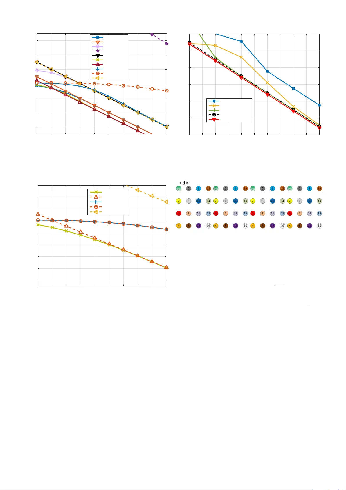
1 This work has been submitted to the IEEE for possible publication. Cop yright may be transferred without notice, after which this version may no longer be accessible. 2 A Frame work for Ov er -the-air Reciprocity Calibration for TDD Massi v e MIMO Systems Xiwen JIANG, Alexis Decurninge, Kalyana Gopala, Florian Kaltenber ger, Member , IEEE, Maxime Guillaud, Senior Member , IEEE, Dirk Slock, F ellow , IEEE, and Luc Deneire, Member , IEEE Abstract —One of the biggest challenges in operating massive multiple-input multiple-output systems is the acquisition of ac- curate channel state information at the transmitter . T o take up this challenge, time division duplex is mor e favorable thanks to its channel reciprocity between downlink and uplink. However , while the propagation channel ov er the air is recipr ocal, the radio-frequency front-ends in the transceivers are not. Therefor e, calibration is requir ed to compensate the RF hardware asymme- try . Although various o ver -the-air calibration methods exist to address the above problem, this paper offers a unified repr esen- tation of these algorithms, pro viding a higher level view on the calibration problem, and introduces innovations on calibration methods. W e present a novel family of calibration methods, based on antenna grouping, which impro ve accuracy and speed up the calibration process compared to existing methods. W e then pro vide the Cram ´ er -Rao bound as the perf ormance ev aluation benchmark and compare maximum likelihood and least squares estimators. W e also differentiate between coher ent and non- coherent accumulation of calibration measurements, and point out that enabling non-coherent accumulation allows the training to be spr ead in time, minimizing impact to the data service. Overall, these results have special value in allowing to design recipr ocity calibration techniques that are both accurate and resour ce-effective. Index T erms —Massive MIMO, TDD, channel reciprocity cal- ibration. I . I N T RO D U C T I O N Massiv e multiple-input multiple-output (MIMO) is a promising air interface technology for the next generation of wireless communications. W ith large number of antennas installed at the base station (BS) simultaneously serving mul- tiple user equipments (UEs), massi ve MIMO can dramatically improv e the spectral efficiency of cellular networks [1], [2]. For downlink (DL), one of the fundamental challenges to fully realize the potential of massiv e MIMO is the acquisition of accurate channel state information at the transmitter (CSIT). T ime division duplex (TDD) thus attracts great attention This work is supported in part by Huawei Mathematical and Algorithmic Sciences Lab in Paris through the project of “Modeling, Calibrating and Exploiting Channel Reciprocity for Massiv e MIMO”. It is partly supported by the French Government (National Research Agency , ANR) through the “In vestments for the Future” Program #ANR-11-LABX-0031-01). X. Jiang, K. Gopala, F . Kaltenberger and D. Slock are with Communication Systems Department, EURECOM. (e-mail: { xiwen.jiang, kalyana.gopala, florian.kaltenberger , dirk.slock } @eurecom.fr) A. Decurninge and M. Guillaud are with the Mathematical and Algorithmic Sciences Lab, Paris Research Center, Huawei T echnologies France. (e-mail: { alexis.decurninge, maxime.guillaud } @huawei.com) L. Deneire is with Laboratoire I3S, Universit ´ e de Nice Sophia Antipolis. (e-mail: luc.deneire@unice.fr) from the research community as it enjoys channel reciprocity between DL and uplink (UL), thanks to which the BS can obtain the CSIT from the channel estimation in the UL. In fact, traditional ways to get CSIT from UE feedback becomes infeasible when the antenna array size at the BS scales up, because of the heavy signaling ov erhead it incurs in the UL. Channel reciprocity in TDD systems refers to the fact that the physical over -the-air (OT A) channels are the same for UL and DL [3], [4] within channel coherence time. Howe ver , the channel as seen by the digital baseband pro- cessor contains not only the physical O T A channel b ut also radio frequency (RF) front-ends, including the hardware from digital-to-analog conv erter (DA C) to transmit antennas at the transmitter (Tx) and the corresponding part, from receiving antennas to analog-to-digital conv erter (ADC), at the receiv er (Rx). The various impairments to reciprocity can be due to manufacturing variability in the power amplifiers and low- noise amplifiers, different cable lengths across the antennas, imperfect clock synchronization, duplexer response, etc. Due to these, the hardware in the Tx and Rx RF chains are, in general, not identical, and therefore the channel from a digital signal processing point of view is not reciprocal. If not taken into account, these hardware-related asymmetries will cause inaccuracy in the CSIT estimation and, as a consequence, seriously degrade the DL beamforming performance [5]–[8]. In order to compensate the hardware asymmetry and restore channel reciprocity , calibration techniques are needed. This topic has been explored long before the advent of massiv e MIMO. In [9]–[13], it is suggested to add additional hardware components in transceivers which are dedicated to calibration. This method (which we refer to as absolute calibration) con- sists in compensating the Tx and Rx RF asymmetry indepen- dently in each transceiv er; ho wever this does not appear to be a cost-effecti ve solution. [14]–[17] thus put forward “relativ e” calibration schemes 1 , where the calibration coef ficients are estimated using signal processing methods based on O T A bi- directional channel estimation between BS and UE. Since hardware properties can be expected to evolv e slo wly , and these coefficients can be obtained in the initialization phase of the system (calibration phase), the y can be used later together with the instantaneous UL channel estimate to obtain do wnlink CSIT . W ith the advent of massive MIMO, traditional relativ e calibration methods are challenged, because they require the 1 The term relative indicates here that the calibration coefficients relate the UL and DL digital channels, as opposed to absolute calibration which relates digital domain and propagation domain versions of a channel. 3 UE to feed back a lar ge amount of DL CSI for all BS antennas. It was observed in [18] that the calibration factor at the BS side is the same for all channels from the BS to any UE. This was exploited in [18] to determine the BS side calibration factor of a secondary BS with the cooperation of a secondary UE, allowing beamforming with zero-forcing to a primary UE without its collaboration. This idea was then pushed further in a number of OT A self-calibration approaches which only require the e xchange of O T A training signals between elements of the BS array . Indeed, for optimizing multi-user massiv e MIMO systems, the asymmetry in the number of antennas between the BS and the UEs means that most of the massive MIMO multi-user multiplexing gain can be achieved through BS-side only calibration [19], [20]. These OT A self-calibration approaches hav e the advantage that, unlik e classical single- link relati ve calibration, no CSI feedback is in volv ed, since all the elements of the BS array are already connected to the same baseband signal processor . Such “single-side” or “internal” calibration methods were proposed in [21]–[25]. In [21], the authors reported on the massiv e MIMO Argos prototype, where calibration is performed O T A with the help of a reference antenna. By performing bi-directional transmission between the reference antenna and the rest of the antenna array , it is possible to estimate the calibration coef ficients up to a common scalar ambiguity which will not influence the final DL beamforming capability . The Argos calibration approach howe ver is sensitiv e to the location of the reference antenna, and as one of the consequences, is not suitable for distrib uted massiv e MIMO. This concern moti v ated the introduction of a method (Rogalin et al. in [22]) whereby calibration is not performed w .r .t. a reference antenna 2 . It has the spirit of distributed algorithms, making it a good calibration method for antenna arrays ha ving a distributed topology . Note that it can also be applied to colocated massi ve MIMO, as in the LuMaMi massive MIMO prototype [26] where a weighted version of the estimator presented in [23] is used, whereas a Maximum Likelihood (ML) estimator is presented in [24]. Moreov er , a fast calibration method named A valanche was proposed in [25]; its principle is to use a calibrated sub-array to calibrate uncalibrated elements. The calibrated array thus grows during the calibration process in a way similar to the av alanche phenomenon. Among other relev ant works, we refer to [27]–[31]. In [27], the author provides an idea to perform system health monitoring on the calibrated reciprocity . Under the assumption that the majority of calibration coefficients stay calibrated and only a minority of them change, the authors propose a compressed sensing enabled detection algorithm to find out which calibration coefficient has changed based on the sparsity in the v ector representing the coefficient change. In [28], a calibration method dedicated to maximum ratio transmission (MR T) is proposed. Experimental data about the calibration coefficients are reported in [21], [29]–[31], gi ving an insight on how the impairments e volve in the time and frequenc y domains 2 The method in [22] is denoted as “least-squares (LS) calibration”, howe ver we will not use this terminology since most calibration techniques proposed in the literature ultimately rely on LS estimation as well as with the temperature, and about the hardware properties behind this effect. In the present article, we introduce a unified framew ork to represent different existing calibration methods. Although they appear at first sight to be different, we re veal that all existing calibration methods can be modeled under a general pilot based calibration framew ork; different ways to partition the array into transmit and recei ve elements during successiv e training phases yield different schemes. The unified represen- tation shows the relationship between these methods and pro- vides alternative ways to obtain corresponding estimators. As this framew ork giv es a general and high level understanding of the TDD calibration problem in massive MIMO systems, it opens up possibilities for new calibration methods. As an example, we present a novel family of calibration schemes based on antenna grouping, which can greatly speed up the calibration process with respect to the classical approaches. W e will show that our proposed method greatly outperforms the A valanche method [25] in terms of calibration accuracy , yet it is equally fast. In order to ev aluate the performance of calibration schemes, we deriv e the Cram ´ er-Rao bounds (CRB) of the accuracy of calibration coefficients estimation. Another important contribution of this work is the introduction of non-coherent accumulation of the measurements used for calibration. W e will see that calibration does not necessarily hav e to be performed in an intensive manner during a single channel coherence interval, but can rather be executed using time resources distributed over a relati vely long period. This enables TDD reciprocity calibration to be interleaved with the normal data transmission or reception, leaving it almost in visible for the whole system. The rest of this paper is organized as follows. Section II de- scribes the basic principles of reciprocity calibration in a TDD based MIMO system. Section III presents the TDD reciprocity system model and introduces our unified framework. Sec- tion IV presents ho w Argos, Rogalin and A v alanche calibration algorithms fit into this model as well as how we can obtain the corresponding estimators. In Section V, we present the fast calibration scheme based on antenna grouping and discuss the minimum number of channel uses it requires to estimate all calibration coef ficients. In Section VI, we address the optimal estimation problem of reciprocity calibration parameters, we deriv e the CRB, propose a maximum likelihood (ML) es- timator and compare it with the LS estimator . Section VII is dedicated to non-coherent accumulation of measurements. In Section VIII, we illustrate the performance of the group- based fast calibration method and compare its performance with other calibration algorithms using CRB as the benchmark. Conclusions are drawn in Section IX. The notation adopted in this paper conforms to the fol- lowing conv entions. V ectors and matrices are denoted in lowercase bold and uppercase bold respectiv ely: a and A . ( · ) ∗ , ( · ) T , ( · ) H , ( · ) † denote element-wise complex conjugate, transpose, Hermitian transpose and Moore-Penrose pseudo in verse, respectiv ely . ⊗ and ∗ denotes the Kronecker product operator and the Khatri–Rao product [32], respectiv ely . d·e is the ceiling operator, which rounds a number to the next integer . diag { a 1 , a 2 , . . . , a M } denotes a diagonal matrix with 4 its diagonal composed of a 1 , a 2 , . . . , a M , whereas vec ( A ) denotes the vectorization of the matrix A . C denotes the set of complex numbers. I I . OT A R E C I P R O C I T Y C A L I B R AT I ON In this section, we describe the basic idea of reciprocity calibration in a practical TDD system. Let us consider a system as in Fig. 1, where A represents a BS and B represents a UE, each containing M A and M B antennas, respectiv ely . The DL and UL channels flat-fading model (as typically obtained by considering a single subcarrier of a multicarrier system) seen in the digital domain are noted by H A → B and H B → A . Since they are formed by the cascade of the Tx impairments, OT A propagation, and Rx impairments, they can be represented by ( H A → B = R B C A → B T A , H B → A = R A C B → A T B , (1) where matrices T A , R A , T B , R B model the response of the transmit and recei ve RF front-ends, while C A → B and C B → A model the OT A propagation channels, respectively from A to B and from B to A. The dimension of T A and R A are M A × M A , whereas that of T B and R B are M B × M B . The diagonal elements in these matrices represent the linear effects attributable to the impairments in the transmitter and receiv er parts of the RF front-ends respecti vely , whereas the off-diagonal elements correspond to RF crosstalk and antenna mutual coupling 3 . It is worth noting that although transmitting and receiving antenna mutual coupling is not generally recip- rocal [34], theoretical modeling [12] and experimental results [21], [24], [31] both sho w that in practice, RF crosstalk and antenna mutual coupling can be ignored for the purpose of reciprocity calibration, which implies that T A , R A , T B , R B can safely be assumed to be diagonal. Assuming the system is operating in TDD mode, the O T A channel responses enjoy reciprocity within the channel coher - ence time, i.e., C A → B = C T B → A . Therefore, we obtain the following relationship between the channels measured in both directions: H A → B = R B ( R − 1 A H B → A T − 1 B ) T T A = R B T − T B | {z } F − T B H T B → A R − T A T A | {z } F A = F − T B H T B → A F A . (2) A system utilizing OT A reciprocity calibration normally has two phases for its function. Firstly , during the initialization of the system, the calibration process is performed, which consists in estimating F A and F B . Then during the data transmission phase, they are used together with instantaneous measured UL channel ˆ H B → A to estimate H A → B according to (2), based on which adv anced beamforming algorithms can be performed. Since the calibration coef ficients typically 3 Here, “antenna mutual coupling” is used to describe parasitic effects that two nearby antennas hav e on each other , when the y are either both transmitting or receiving [12], [33]. Howe ver, this is different to the channel between transmitting and receiving elements of the same array , which we call the intra-array channel. Note that this differs from the terminology in [24] and [28] where the term mutual coupling is used to denote the intra-array channel. R A C A → B C B → A R B T B A B H A → B H B → A T A Fig. 1. Reciprocity Model remain stable [21], the calibration process does not hav e to be performed very frequently . Note that the studies in [19], [20] pointed out that in a practical multi-user MIMO system, it is mainly the calibration at the BS side which restores the hardware asymmetry and helps to achie ve the multi-user MIMO performance, whereas the benefit brought by the calibration on the UE side is not necessarily justified. W e thus, in the sequel, focus on the estimation of F A , although the frame work discussed in the following section is not limited to this case. I I I . G E N E R A L OTA C A L I B R AT I O N F R A M E W O R K A. Overview and signalling In this section, we present a general frame work for O T A pilot-based reciprocity calibration. Let us consider an antenna array of M elements partitioned into G groups denoted by A 1 , A 2 , . . . , A G , as in Fig. 2. Group A i contains M i antennas such that P G i =1 M i = M . Each group A i transmits a sequence of L i pilot symbols, defined by matrix P i ∈ C M i × L i where the rows correspond to antennas and the columns to successive channel uses. Note that a channel use can be understood as a time slot or a subcarrier in an OFDM-based system, as long as the calibration parameter can be assumed constant ov er all channel uses. When an antenna group i transmits, all other groups are considered in receiving mode. After all G groups hav e transmitted, the receiv ed signal for each resource block of bidirectional transmission between antenna groups i and j is gi ven by  Y i → j = R j C i → j T i P i + N i → j , Y j → i = R i C j → i T j P j + N j → i , (3) where Y i → j ∈ C M j × L i and Y j → i ∈ C M i × L j are received signal matrices at antenna groups j and i respecti vely when the other group is transmitting. N i → j and N j → i represent the corresponding receiv ed noise matrix. T i , R i ∈ C M i × M i and T j , R j ∈ C M j × M j represent the effect of the transmit and receiv e RF front-ends of antenna elements in groups i and j respectiv ely . The reciprocity property induces that C i → j = C T j → i , thus for tw o dif ferent groups 1 ≤ i 6 = j ≤ G , by eliminating C i → j in (3) we have P T i F T i Y j → i − Y T i → j F j P j = e N ij , (4) where the noise component e N ij = P T i F T i N j → i − N T i → j F j P j , while F i = R − T i T i and F j = R − T j T j are the calibration ma- trices for groups i and j . The calibration matrix F is diagonal, 5 Fig. 2. Bi-directional transmission between antenna groups. and thus takes the form of F = diag { F 1 , F 2 , . . . , F G } . Note that estimating F i or F j from (4) for a given pair ( i, j ) does not exploit all rele vant receiv ed data. An optimal estimation jointly considering all recei ved signals for all ( i, j ) will be proposed in Section VI. Note that the proposed framework also allows to consider using only subsets of the received data which corresponds to some of the methods found in the literature. Let us use f i and f to denote the vectors of the diagonal coefficients of F i and F respectiv ely , i.e., F i = diag { f i } and F = diag { f } . This allows us to vectorize (4) into ( Y T j → i ∗ P T i ) f i − ( P T j ∗ Y T i → j ) f j = e n ij , (5) where ∗ denotes the Khatri–Rao product (or column-wise Kronecker product 4 ), where we ha ve used the equality vec ( A diag ( x ) B ) = ( B T ∗ A ) x . Note that, if we do not suppose that ev ery F i is diagonal, (5) holds more generally by replacing the Katri–Rao products by Kroneck er products and f i by vec ( F i ) . Finally , stacking equations (5) for all 1 ≤ i < j ≤ G yields Y ( P ) f = e n , (6) with Y ( P ) defined as      ( Y T 2 → 1 ∗ P T 1 ) − ( P T 2 ∗ Y T 1 → 2 ) 0 . . . ( Y T 3 → 1 ∗ P T 1 ) 0 − ( P T 3 ∗ Y T 1 → 3 ) . . . 0 ( Y T 3 → 2 ∗ P T 2 ) − ( P T 3 ∗ Y T 2 → 3 ) . . . . . . . . . . . . . . .      | {z } ( P G j =2 P j − 1 i =1 L i L j ) × M . (7) It is worth noting that this framew ork is not limited to represent single-side calibration. For UE-aided (relativ e) cal- ibration, it suf fices to set 2 groups such as A 1 and A 2 , representing the BS and the UE, respectively in order to get a full calibration scheme. 4 W ith matrices A and B partitioned into columns, A =  a 1 a 2 . . . a M  and B =  b 1 b 2 . . . b M  where a i and b i are column vectors for i ∈ 1 . . . M , then, A ∗ B =  a 1 ⊗ b 1 a 2 ⊗ b 2 . . . a M ⊗ b M  [32]. B. P arameter identifiability and pilot design Before proposing an estimator for f , we raise the question of the problem identifiability which corresponds to the fact that (6) admits a unique solution in the noiseless scenario Y ( P ) f = 0 . (8) The solution of (8) is defined up to a complex scalar factor α , since if f is a solution, then α f is also a solution of (8). This indeterminacy can be resolv ed by fixing one of the calibration parameters, say f 1 = e H 1 f = [1 0 · · · 0] f = 1 or by a norm constraint, for e xample k f k = 1 . Then, the identifiability is related to the dimension of the kernel of Y ( P ) in the sense that the problem is fully determined if and only if the kernel of Y ( P ) is of dimension 1 . Since the true f is a solution to (8), we know that the rank of Y ( P ) is at most M − 1 . W e will assume furthermore in the following that the pilot design is such that the rows of Y ( P ) are linearly independent as long as the number of rows is less than M − 1 . Note that this condition depends on the internal channel realization C i → j and on the pilot matrices P i . Howe ver , sufficient conditions of identifiability expressed on these matrices are out of the scope of this paper . Under rows independence, (6) may be read as the following sequence of events: 1) Group 1 broadcasts its pilots to all other groups using L 1 channel uses; 2) After group 2 transmits its pilots, we can formulate L 2 L 1 equations of the form (5); 3) After group 3 transmits its pilots, we can formulate L 3 L 1 + L 3 L 2 equations; 4) After group j transmits its pilots, we can formulate P j − 1 i =1 L j L i equations. This process continues until group G finishes its transmission, and the whole calibration process finishes. During this process of transmission by the G antenna groups, we can start forming equations as indicated, that can be solved recursively for subsets of unknown calibration parameters, or we can wait until all equations are formed to solve the problem jointly . By independence of the rows, we can state that the problem is fully determined if and only if X 1 ≤ i M − 1 = 63 . This means that the proposed fast calibration, which exploits all data jointly for the parameter estimation, has an advantage over the A valanche method which solves exactly determined subsets of equations and hence suffers from error propagation. Also, the performance impro ves when the group sizes are allocated more equitably as in grouping scheme FC-II. Intuitiv ely , the overall estimation performance of the fast calibration would be limited by the (condition number of the) largest group size and hence it is reasonable to use a grouping scheme that tries to minimize the size of the largest antenna group. These observations hold irrespectiv e of the constraints used. A valanche with the FCC constraint exhibits a huge MSE and hence most portions of this curve fall outside the range of Fig. 6. Note also that the MSE in some cases falls below the CRB, see for instance the MSE NPC FC-I curve at low SNRs. This is because in this SNR re gion the MSE saturates due to bias and the CRB is no longer applicable as explained in Section VI-D. It is also illustrativ e to consider the case of M = 67 antennas, which is the maximum number of antennas that can be calibrated with G = 12 channel uses. As shown in section V, the best strategy is to divide the antennas into G = 12 groups and letting each group transmit exactly once ( L i = 1 ). This then results in a linear system of 66 equations (6) plus one constraint in 67 unknowns. Indeed, (9) yields 66 = 1 2 G ( G − 1) = M − 1 = 66 . Thus, the system of equations is exactly determined by using an appropriate constraint to resolve the scale factor ambiguity . Hence, the error attained by any LS solution would be zero and the different constraints used for estimation would only lead to different scale factors in the calibration parameter estimates. So, all the solutions would be equiv alent. Also, FC-I grouping leads to a block triangular structure with square diagonal blocks for the matrix Y defined in (7) after removing the first column. Hence, the back substitution based solution performed by A v alanche is indeed the ov erall LS solution with the first coef ficient known constraint. Thus, in Fig. 7 where the performance of these schemes is compared for M = 67 , we see that the curves for A valanche and fast calibration with the FC-I grouping overlap completely . In general, this beha vior would occur whenev er the number of antennas corresponds to the maximum that can be calibrated with the number of channel uses (see Sec. III-B), and the antenna grouping is similar to that for FC-I. At the range of SNRs considered, the MSE is saturated and is hence far below the CRB for this grouping. In fact, only a part of the CRB for the FC-I grouping can be seen as the rest of the curve falls outside the range of the figure. Indeed, though not shown in Fig. 7, the MSE curve with the FC-I grouping only starts to ov erlap with the corresponding CRB curve for SNR beyond 100dB! Howe ver , it is important to note that the performance improv es dramatically with a more equitable grouping of the antennas as can be seen from the curves for the FC-II grouping in the same figure. In Fig. 8, we consider slower transmit schemes that transmit from one antenna at a time ( G = M ) and compare their MSE performance with the CRB. The MSE with FCC for Argos, Rogalin [22] and the AML method in Algorithm 1 is plotted. As expected, the Rogalin method improves o ver Argos by using all the bi-directional receiv ed data. AML 12 5 10 15 20 25 30 35 40 45 50 SNR(dB) -10 0 10 20 30 40 50 MSE in dB MSE FCC FC-II CRB FCC FC-II MSE FCC FC-I MSE FCC Avl CRB FCC FC-I MSE NPC FC-II CRB NPC FC-II MSE NPC FC-I MSE NPC Avl CRB NPC FC-I Fig. 6. Comparison of fast calibration with A valanche scheme ( M = 64 and the number of channel use is 12). The curves are averaged across 500 channel realizations. The performance with both the FCC and NPC constraints is shown. 15 20 25 30 35 40 45 50 55 60 SNR(dB) -30 -20 -10 0 10 20 30 40 50 MSE in dB MSE NPC FC-II CRB NPC FC-II MSE NPC FC-I MSE NPC Avl CRB NPC FC-I Fig. 7. Comparison of fast calibration with A valanche scheme for M = 67 and number of channel uses 12. The curves are averaged across 500 channel realizations. The NPC constraint is used for the MSE computation. outperforms the Rogalin performance at low SNR. These curves are compared with the CRB deriv ed in VI-A for the FCC case and it can be seen that the AML curve overlaps with the CRB at higher SNRs. Also plotted is the CRB as giv en in [24] assuming the internal propagation channel is fully known (the mean is kno wn and the v ariance is ne gligible) and the underestimation of the MSE can be observed as expected. T o bring out the dif ference between the two CRB deri v ations, the amplitude variation parameter δ is chosen to be 0.5 to increase the range of values of Tx and Rx calibration parameters. So far , we hav e focused on an i.i.d. intra-array channel model and we hav e seen in Fig. 6 and Fig. 7 that the size of the transmission groups is an important parameter that impacts the MSE of the calibration parameter estimates. W e 0 5 10 15 20 25 30 35 40 45 50 SNR(dB) -40 -30 -20 -10 0 10 20 MSE in dB MSE - Argos MSE - Method in [22] MSE - AML CRB CRB in [24] Fig. 8. Comparison of single antenna transmit schemes with the CRB ( G = M = 16 ). The curves are generated over one realization of an i.i.d. Rayleigh channel and known first coefficient constraint is used. Fig. 9. 64 antennas arranged as a 4 × 16 grid. now consider a more realistic scenario where the intra-array channel is based on the geometry of the BS antenna array and make some observations on the choice of the antennas to form a group. W e consider an array of M = 64 antennas arranged as in Fig. 9. The path loss (4 π d i → j λ ) 2 between any two antennas i and j is a function of their distance d i → j , and λ is the wa velength of the recei ved signal. In the simulations, the distance between adjacent antennas, d , is chosen as λ 2 . The phase of the channel between any two antennas is modeled to be a uniform random v ariable in [ − π , π ] . Such a model was also observed experimentally in [24]. The SNR is defined as the signal to noise ratio observed at the receive antenna nearest to the transmitter . Continuing with the same internal channel model, consider a scenario in which antennas transmit in G = 16 groups of 4 each. Note that this is not the fastest grouping possible, but the example is used for the sake of illustration. W e consider two different choices to form the antenna groups: 1) interleav ed grouping corresponding to selecting antennas with the same numbers into one group as in Fig. 9, 2) non-interleaved grouping corresponding to selecting antennas in each column as a group. Fig. 10 shows that interleaving of the antennas results in performance gains of about 10dB. Intuitiv ely , the interleaving of the antennas ensures that the channel from a group to the rest of the antennas is as well conditioned as possible. This example clearly sho ws that in addition to the 13 0 5 10 15 20 25 30 35 40 45 50 SNR(dB) -30 -20 -10 0 10 20 30 40 50 MSE in dB MSE interleaved CRB interleaved MSE non-interleaved CRB non-interleaved Fig. 10. Interleaved and non-interleaved MSE and CRB with NPC for an antenna transmit group size of 4 ( M = 64 and the number of channel uses is G = 16 ). size of the antenna groups, the choice of the antennas that go into each group also has a significant impact on the estimation quality of the calibration parameters. I X . C O N C L U S I O N S In this work we presented an OT A calibration frame work which unifies existing calibration schemes. This framew ork opens up new calibration possibilities. As an example, we proposed a f amily of f ast calibration schemes based on antenna grouping. The number of channel uses needed for the whole calibration process is of the order of the square root of the antenna array size rather than scaling linearly . In fact it can be as fast as the existing A v alanche calibration method, b ut av oiding the sev ere error propagation problem, thus greatly outperforming the A v alanche method, as has been shown by simulation results. W e also presented a simple CRB formulation for the es- timation of the relativ e calibration parameters. As the group calibration formulation encompasses the existing calibration methods, the CRB computation can be used to e valuate existing state of the art calibration methods as well. W e then proposed a ML estimator and reveal the relationship between ML and LS estimation. Moreov er , we differentiated the notions of coherent and non-coherent accumulations for calibration observ ations. W e illustrated that it is possible to perform calibration measure- ments using time slots that can be sparsely distributed over a relativ ely long time. This makes the calibration process consume a vanishing fraction of channel use resources and allows to minimize the impact on the ongoing data service. As illustrated by simulations, for the fast calibration, inter- leav ed grouping has a better performance than non-interleaved grouping. Howe ver , the best antenna group definitions for giv en antenna group sizes is still an open question. Addition- ally , the optimal pilot design for calibration is unknown, which is an interesting topic for future work. A P P E N D I X A O P T I M A L G R O U P I N G Lemma 1. F ix K ≥ 1 . Let us define an optimal gr ouping as the solution G ∗ , L ∗ 1 , . . . , L ∗ G ∗ of max P G i =1 L i = K X i 1 . W ithout loss of generality , we can suppose that L G > 1 . Then, we can break up group G and add one group which contains a single antenna, i.e., let us consider L 0 = ( L 1 , . . . , L G − 1 , 1) . In that case, it holds P G i =1 L i = P G +1 i =1 L 0 i = K and G +1 X j =2 j − 1 X i =1 L 0 j L 0 i = G − 1 X j =2 j − 1 X i =1 L 0 j L 0 i + ( L 0 G + L 0 G +1 ) G − 1 X i =1 L 0 j L 0 i + L 0 G L 0 G +1 = G X j =2 j − 1 X i =1 L j L i + L 0 G > G X j =2 j − 1 X i =1 L j L i which contradicts the fact that L is solution to (41). W e conclude therefore that L j = 1 for any j and G ∗ = K . A P P E N D I X B C O N S T RU C T I O N O F F ⊥ W e show in the following that the column space of F ⊥ defined by (36) spans the orthogonal complement of the column space of F assuming that P i is full rank for all i and that either L i ≥ M i or M i ≥ L i for all i. Pr oof. First, using ( A ⊗ B )( C ⊗ D ) = ( AC ⊗ BD ) , it holds  I L i ⊗ P T j F j − P T i F i ⊗ I L j  | {z } L i L j × ( L i M j + L j M i )  P T i F i ⊗ I M j I M i ⊗ P T j F j  | {z } ( L i M j + L j M i ) × M i M j = 0 . (42) Then, the ro w space of the left matrix of (42) is orthogonal to the column space of the right matrix. As F in (29) and F ⊥ H are block diagonal with blocks of the form of (42), it suffices then to prove that the following matrix M has full column rank, i.e., L i M j + L j M i , which is then also its row rank M :=  I L i ⊗ P T j F j − P T i F i ⊗ I L j ( F i P i ) ∗ ⊗ I M j I M i ⊗ ( F j P j ) ∗  . (43) Denote A i := P T i F i ∈ C L i × M i and A j := P T j F j ∈ C L j × M j . Then, by assumption, it holds that either rank ( A i ) = M i and rank ( A j ) = M j or rank ( A i ) = L i and rank ( A j ) = 14 L j . Let x = [ x T 1 x T 2 ] T be such that Mx = 0 and show that x = 0 . Since Mx = 0 , it holds  ( I L i ⊗ A j ) x 1 − ( A i ⊗ I L j ) x 2 = 0 ( A H i ⊗ I M j ) x 1 + ( I M i ⊗ A j ) x 2 = 0 . Let X 1 and X 2 be matrices such that vec ( X 1 ) = x 1 and vec ( X 2 ) = x 2 . Then  A j X 1 − X 2 A T i = 0 X 1 A ∗ i + A H j X 2 = 0 . Multiplying the first equation by A H j and the second by A T i , and summing them up, we get A H j A j X 1 + X 1 ( A i A H i ) ∗ = 0 , which is a Sylvester’ s equation admitting a unique solution if A H j A j and − ( A i A H i ) ∗ hav e no common eigen values. On the other hand, the eigen values of A H j A j and A i A H i are real positiv e, so common eigen v alues of A H j A j and − ( A i A H i ) ∗ can only be 0 . Howe ver , this does not occur since by the assumptions either A H j A j or A i A H i is full rank. W e can then conclude that X 1 = 0 , i.e., x 1 = 0 . Similarly , x 2 = 0 , which ends the proof. R E F E R E N C E S [1] T . Marzetta, “Noncooperative cellular wireless with unlimited numbers of base station antennas, ” IEEE T rans. Wir eless Commun. , vol. 9, no. 11, pp. 3590–3600, Nov . 2010. [2] E. Larsson, O. Edfors, F . Tufv esson, and T . Marzetta, “Massive MIMO for next generation wireless systems, ” IEEE Commun. Mag . , vol. 52, no. 2, pp. 186–195, Feb. 2014. [3] H. A. Lorentz, “het theorema van Poynting over energie in het electro- magnetisch veld en een paar algemeene stellingen over de voorplanting van het licht, ” in V ersl. K on. Akad. W entensch. Amster dam , 1896, p. 176. [4] G. Smith, “ A direct deriv ation of a single-antenna reciprocity relation for the time domain, ” IEEE T rans. on Antennas and Pr opagation , vol. 52, no. 6, pp. 1568–1577, Jun. 2004. [5] J. C. Guey and L. D. Larsson, “Modeling and ev aluation of MIMO systems exploiting channel reciprocity in TDD mode, ” in Pr oc. IEEE 60th V eh. T echnol. Conf. (VTC) , vol. 6, 2004, pp. 4265–4269. [6] X. Luo, “Multi-user massive MIMO performance with calibration er- rors, ” IEEE Tr ans. on W ir eless Commun. , vol. 15, no. 7, July 2016. [7] W . Zhang, H. Ren, C. Pan, M. Chen, R. C. de Lamare, B. Du, and J. Dai, “Large-scale antenna systems with UL/DL hardware mismatch: achiev able rates analysis and calibration, ” IEEE T rans. on Commun. , vol. 63, no. 4, pp. 1216–1229, 2015. [8] X. Jiang, F . Kaltenberger , and L. Deneire, “How accurately should we calibrate a massive MIMO TDD system?” in Proc. IEEE Intern. Conf. on Commun. (ICC) W orkshops , 2016. [9] A. Bourdoux, B. Come, and N. Khaled, “Non-reciprocal transceivers in OFDM/SDMA systems: impact and mitigation, ” in Proc. IEEE Radio and W ireless Conf. (RA WCON) , Boston, MA, USA, Aug. 2003, pp. 183– 186. [10] K. Nishimori, K. Cho, Y . T akatori, and T . Hori, “ Automatic calibra- tion method using transmitting signals of an adaptive array for TDD systems, ” Pr oc. IEEE T rans. on V eh. T echnol. , vol. 50, no. 6, pp. 1636– 1640, 2001. [11] K. Nishimori, T . Hiraguri, T . Ogawa, and H. Y amada, “Effecti veness of implicit beamforming using calibration technique in massive MIMO system, ” in Proc. IEEE Intern. W orkshop on Electr omagnetics (iWEM) , 2014, pp. 117–118. [12] M. Petermann, M. Stefer , F . Ludwig, D. W ¨ ubben, M. Schneider , S. Paul, and K. Kammeyer , “Multi-user pre-processing in multi-antenna OFDM TDD systems with non-reciprocal transceivers, ” IEEE T rans. Commun. , vol. 61, no. 9, pp. 3781–3793, Sep. 2013. [13] A. Benzin and G. Caire, “Internal self-calibration methods for large scale array transceiv er software-defined radios, ” in 21th International ITG W orkshop on Smart Antennas (WSA) , Berlin, Germany , Mar . 2017. [14] M. Guillaud, D. Slock, and R. Knopp, “ A practical method for wireless channel reciprocity exploitation through relativ e calibration, ” in Proc. Intern. Symp. Signal Pr ocess. and Its Applications , Sydney , Australia, Aug. 2005, pp. 403–406. [15] F . Kaltenberger, H. Jiang, M. Guillaud, and R. Knopp, “Relativ e channel reciprocity calibration in MIMO/TDD systems, ” in Pr oc. Futur e Network and Mobile Summit , Florence, Italy , Jun. 2010, pp. 1–10. [16] J. Shi, Q. Luo, and M. Y ou, “ An efficient method for enhancing TDD over the air reciprocity calibration, ” in Proc. IEEE Wir eless Commun. and Netw . Conf. , 2011, pp. 339–344. [17] B. Kouassi, I. Ghauri, B. Zayen, and L. Deneire, “On the performance of calibration techniques for cognitive radio systems, ” in Pr oc. IEEE W ireless P ersonal Multimedia Commun. (WPMC) , Oct. 2011, pp. 1–5. [18] B. Kouassi, B. Zayen, R. Knopp, F . Kaltenberger , D. Slock, I. Ghauri, F . Negro, and L. Deneire, “Design and Implementation of Spatial Inter- weav e L TE-TDD Cogniti ve Radio Communication on an Experimental Platform, ” IEEE Wir eless Commun. Mag. , vol. 20, no. 2, 2013. [19] R1-091794, “Hardware calibration requirement for dual layer beamform- ing, ” Huawei, 3GPP RAN1 #57, San Francisco, USA, May 2009. [20] R1-091752, “Performance study on Tx/Rx mismatch in L TE TDD dual- layer beamforming, ” Nokia, Nokia Siemens Networks, CA TT , ZTE, 3GPP RAN1 #57, San Francisco, USA, May 2009. [21] C. Shepard, N. Y u, H.and Anand, E. Li, T . Marzetta, R. Y ang, and L. Zhong, “ Argos: Practical many-antenna base stations, ” in Pr oc. ACM Intern. Conf. Mobile Computing and Netw . (Mobicom) , Istanbul, T urkey , Aug. 2012, pp. 53–64. [22] R. Rogalin, O. Bursalioglu, H. Papadopoulos, G. Caire, A. Molisch, A. Michaloliakos, V . Balan, and K. Psounis, “Scalable synchronization and reciprocity calibration for distributed multiuser MIMO, ” IEEE T rans. W ireless Commun. , vol. 13, no. 4, pp. 1815–1831, Apr. 2014. [23] J. V ieira, F . Rusek, and F . Tufv esson, “Reciprocity calibration methods for massive MIMO based on antenna coupling, ” in Pr oc. IEEE Global Commun. Conf. (GLOBECOM) , Austin, USA, 2014, pp. 3708–3712. [24] J. V ieira, F . Rusek, O. Edfors, S. Malkowsk y , L. Liu, and F . Tufv esson, “Reciprocity Calibration for Massive MIMO: Proposal, Modeling and V alidation, ” IEEE T rans. W ireless Commun. , May 2017. [25] H. Papadopoulos, O. Y . Bursalioglu, and G. Caire, “ A valanche: Fast RF calibration of massiv e arrays, ” in Pr oc. IEEE Global Conf. on Signal and Information Pr ocess. (GlobalSIP) , W ashington, DC, USA, Dec. 2014, pp. 607–611. [26] J. V ieira, S. Malkowsk y , Z. Nieman, K.and Miers, N. Kundargi, L. Liu, I. W ong, V . Owall, O. Edfors, and F . Tufv esson, “ A flexible 100-antenna testbed for massiv e MIMO, ” in Pr oc. IEEE Global Commun. Conf. (GLOBECOM) W orkshops , Austin, USA, 2014, pp. 287–293. [27] X. Luo, “Robust large scale calibration for massive MIMO, ” in Pr oc. IEEE Global Commun. Conf. (GLOBECOM) , San Diego, CA, USA, December 2015, pp. 1–6. [28] H. W ei, D. W ang, H. Zhu, J. W ang, S. Sun, and X. Y ou, “Mutual coupling calibration for multiuser massiv e MIMO systems, ” IEEE T rans. on Wir eless Commun. , vol. 15, no. 1, pp. 606–619, 2016. [29] G. V . Tsoulos and M. A. Beach, “Calibration and linearity issues for an adaptiv e antenna system, ” in Pr oc. IEEE 47th V eh. T echnol. Conf. , vol. 3, May 1997, pp. 1597–1600. [30] G. V . Tsoulos, J. McGeehan, and M. A. Beach, “Space division multiple access (SDMA) field trials. 2. calibration and linearity issues, ” IEE Proc. Radar , Sonar and Navigation , vol. 145, no. 1, pp. 79–84, 1998. [31] X. Jiang, M. ˇ Cirki ´ c, F . Kaltenberger , E. G. Larsson, L. Deneire, and R. Knopp, “MIMO-TDD reciprocity and hardware imbalances: experimental results, ” in Pr oc. IEEE Intern. Conf. on Commun. (ICC) , London, United Kingdom, Jun. 2015, pp. 4949–4953. [32] C. Khatri and C. R. Rao, “Solutions to some functional equations and their applications to characterization of probability distributions, ” Sankhy ¯ a: The Indian Journal of Statistics, Series A , pp. 167–180, 1968. [33] C. A. Balanis, Antenna theory: analysis and design . John Wile y & Sons, 2016. [34] H. W ei, W . D., and X. Y ou, “Reciprocity of mutual coupling for TDD massiv e MIMO systems, ” in Pr oc. Intern. Conf. on W ireless Commun. and Signal Process. (WCSP) , Nanjing, China, Oct. 2015, pp. 1 – 5. [35] R. Rogalin, O. Y . Bursalioglu, H. C. Papadopoulos, G. Caire, and A. F . Molisch, “Hardware-impairment compensation for enabling distributed large-scale MIMO, ” in Pr oc. Information Theory and Applications (IT A) W orkshop, 2013 , San Diego, California, USA., Feb. 2013, pp. 1–10. [36] E. de Carvalho and D. Slock, Semi–Blind Methods for FIR Multichannel Estimation . Prentice Hall, 2000, ch. 7. [Online]. A vailable: http://www .eurecom.fr/publication/469 [37] E. de Carvalho, S. Omar , and D. Slock, “Performance and complexity analysis of blind FIR channel identification algorithms based on deterministic maximum likelihood in SIMO systems, ” Circuits, Systems, and Signal Processing , vol. 34, no. 4, Aug. 2012. [Online]. A vailable: http://www .eurecom.fr/fr/publication/3790 15 [38] E. de Carv alho and D. Slock, “Blind and semi-blind FIR multichannel estimation: (Global) identifiability conditions, ” IEEE T rans. Sig. Proc. , Apr . 2004. [39] ——, “Cram ´ er-Rao bounds for blind multichannel estimation, ” arXiv:1710.01605 [cs.IT], 2017. [Online]. A vailable: https://arxiv .org/ abs/1710.01605 [40] E. de Carvalho, J. Cioffi, and D. Slock, “Cram ´ er-Rao bounds for blind multichannel estimation, ” in Pr oc. IEEE Global Commun. Conf. (GLOBECOM) , San Francisco, CA, USA, Nov . 2000. [41] Z. Jiang and S. Cao, “ A novel TLS-based antenna reciprocity calibration scheme in TDD MIMO systems, ” IEEE Commun. Letters , vol. PP , no. 99, 2016.