Evolution of Social Power in Social Networks with Dynamic Topology

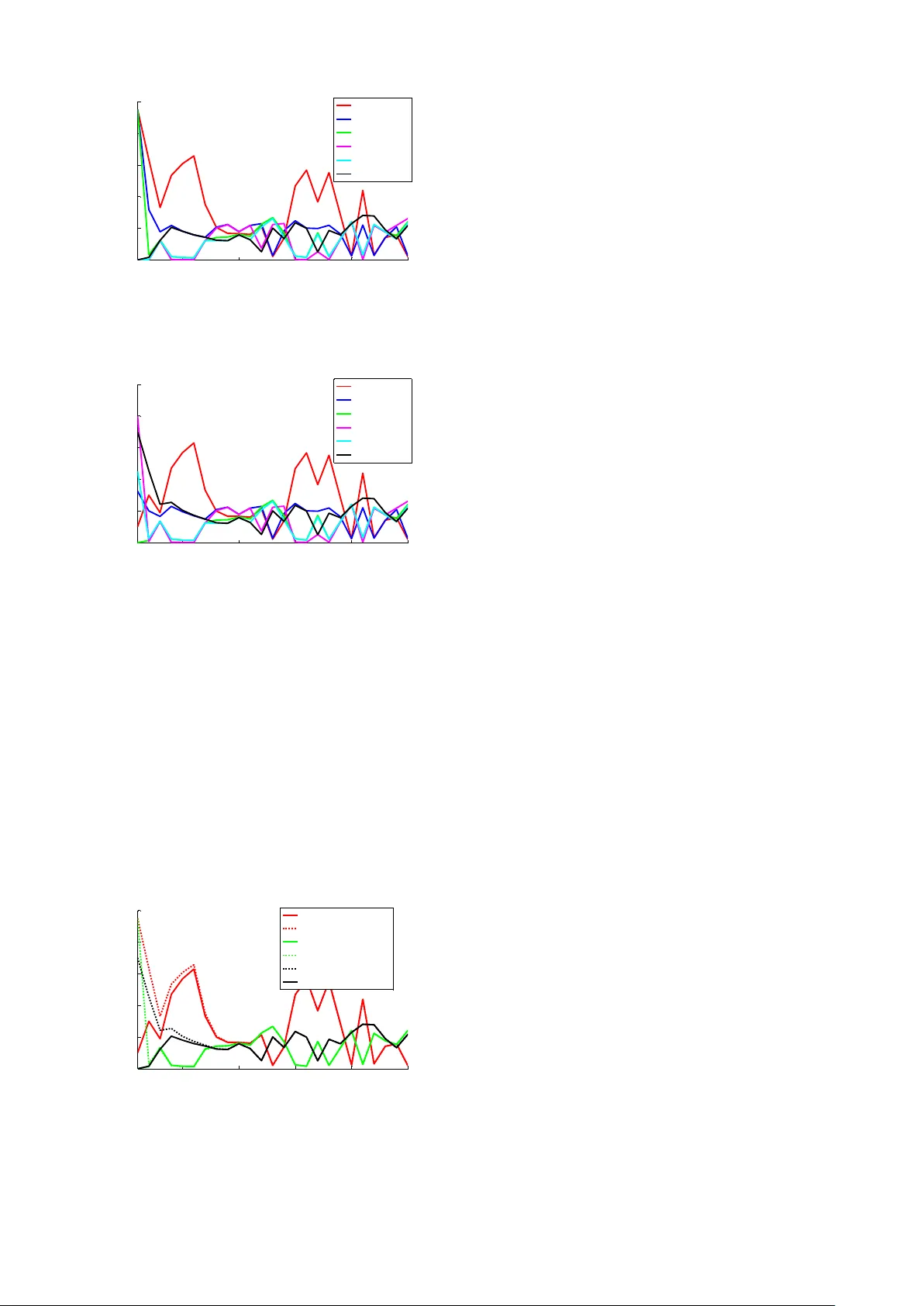
1 Ev olution of Social Po wer in Social Netw orks with Dynamic T opology Mengbin Y e, Student Member , IEEE Ji Liu, Member , IEEE Brian D.O. Anderson, Life F ellow , IEEE Changbin Y u, Senior Member , IEEE T amer Bas ¸ ar , Life F ellow , IEEE Abstract —The recently pr oposed DeGroot-Friedkin model de- scribes the dynamical evolution of indi vidual social power in a social network that holds opinion discussions on a sequence of different issues. This paper r evisits that model, and uses nonlinear contraction analysis, among other tools, to establish several novel results. First, we show that f or a social network with constant topology , each individual’s social power con verges to its equilibrium value exponentially fast, whereas pr evious results only concluded asymptotic conver gence. Second, when the network topology is dynamic (i.e., the relati ve interaction matrix may change between any two successive issues), we show that each individual exponentially for gets its initial social power . Specifically , individual social power is dependent only on the dynamic network topology , and initial (or perceived) social power is forgotten as a result of sequential opinion discussion. Last, we pro vide an explicit upper bound on an individual’ s social power as the number of issues discussed tends to infinity; this bound depends only on the network topology . Simulations are provided to illustrate our results. Index T erms —opinion dynamics, social networks, influence networks, social power , dynamic topology , nonlinear contraction analysis, discrete-time systems I . I N T R O D U C T I O N S OCIAL network analysis is the study of a group of social actors (individuals or organisations) who interact in some way according to a social connection or relationship. The study of social networks has spanned several decades [1], [2] and across sev eral scientific communities. In the past few years, perhaps in part due to lessons learned and tools dev eloped from extensi ve research on coordination of autonomous multi-agent systems [3], the systems and control community has taken an interest in social network analysis. Of particular interest in this context is the problem of “opinion dynamics”, which is the study of how individuals in a social network interact and exchange their opinions on an issue or topic. A critical aspect is to dev elop models which simultaneously capture observed social phenomena and are simple enough to be analysed, particularly from a system-theoretic point of view . The seminal works of [4], [5] proposed a discrete-time opinion pooling/updating rule, now known as the French-DeGroot (or simply DeGroot) model. A continuous-time counterpart, known as the Abelson model, M. Y e, B.D.O. Anderson and C. Y u are with the Research School of Engineering, Australian National University { Mengbin.Ye, Brian.Anderson, Brad.Yu } @anu.edu.au . B.D.O. Anderson is also with Hangzhou Dianzi University , Hangzhou, China, and with Data61-CSIRO (formerly NICT A Ltd.) in Canberra, A.C.T ., Australia. J. Liu and T . Bas ¸ar are with the Coordinated Science Laboratory , University of Illinois at Urbana- Champaign { jiliu, basar1 } @illinois.edu . was proposed in [6]. These opinion updating rules are closely related to consensus algorithms for coordinating autonomous multi-agent systems [7], [8]. The Friedkin-Johnsen model [9], [10] extended the French-DeGroot model by introducing the concept of a “stubborn individual”, i.e., an individual who remains attached to its initial opinion. This helped to model so- cial cleavage [2], a phenomenon where opinions tend towards separate clusters. Other models which attempt to explain social cleav age include the Altafini model with negati ve/antagonistic interactions [11]–[14] and the Hegelsmann-Krause bounded confidence model [15], [16]. Simultaneous opinion discussion on multiple, logically interdependent topics was studied with a multidimensional Friedkin-Johnsen model [17], [18]. The concept of social power or social influence has been integral throughout the dev elopment of these models. Indeed, French Jr’ s seminal paper [4] was an attempt to quantitativ ely study an individual’ s social power in a group discussion. Broadly speaking, in the context of opinion dynamics, individ- ual social power is the amount of influence an individual has on the overall opinion discussion. Individuals which maximise the spread of an idea or rumour in diffusion models were identified in [19]. The social power of an individual in a group can change over time as group members interact and are influenced by each other . Recently , the DeGroot-Friedkin model was proposed in [20] to study the dynamic e volution of an individual’ s social po wer as a social network discusses opinions on a sequence of issues. In this paper, we present sev eral major , nov el results on the DeGroot-Friedkin model. In Section II, we shall provide a precise mathematical formu- lation of the model, but here we provide a brief description to better motiv ate the study , and elucidate the contributions of the paper . The discrete-time DeGroot-Friedkin model [20] is a two- stage model. In the first stage, indi viduals update their opinions on a particular issue, and in the second stage, each individual’ s lev el of self-confidence for the next issue is updated. For a giv en issue, the social network discusses opinions using the DeGroot opinion updating model, which has been em- pirically sho wn to outperform Bayesian learning methods in the modelling of social learning processes [21]. The row- stochastic opinion update matrix used in the DeGroot model is parametrised by two sets of variables. The first is individual social powers, which are the diagonal entries of the opinion update matrix (i.e. the weight an individual places on its own opinion). The second is the relativ e interaction matrix, which is used to scale the off-diagonal entries of the opinion update matrix to ensure that, for any giv en values of individual social 2 powers, the opinion update matrix remains row-stochastic. In the original model [20], the relativ e interaction matrix was assumed to be constant ov er all issues, and constant throughout the opinion discussion on any given issue. Under some mild conditions on the entries of the relati ve interaction matrix, the opinions reach a consensus on ev ery issue. At the end of the period of discussion of an issue, i.e., when opinions ha ve effecti vely reached a consensus, each indi vidual undergoes a sociological process of self-appraisal (detailed in the seminal work [22]) to determine its impact or influence on the final consensus value of opinion. Such a mechanism is well accepted as a hypothesis [23], [24] and has been empirically validated [25]. Immediately before discussion on the next issue, each individual self-appraises and updates its individual social power (the weight an individual places on its own opinion) according to the impact or influence it had on discussion of the previous issue. In updating its individual social power , an individual also updates the weight it accords its neighbours’ opinions, by scaling using the relative interac- tion matrix, to ensure that the opinion updating matrix for the next issue remains row-stochastic. This process is repeated as issues are discussed in sequence. The primary objectiv e of the DeGroot-Friedkin model is to study the dynamical evolution of the individual social powers over the sequence of discussed issues. The model is centralised in the sense that individuals are able to observe and detect their impact relative to ev ery other individual in the opinion discussions process, which indicates that the DeGroot-Friedkin model is best suited for networks of small or moderate size. Such networks are found in many decision making groups such as boards of directors, gov ernment cabinets or jury panels. Distrib uted models of self- appraisal hav e been studied in continuous time [26] as well as discrete time [27], [28] to extend the original DeGroot- Friedkin model. Dynamic topology , b ut restricted to doubly- stochastic relativ e interaction matrices, was studied in [28]. A. Contributions of This P aper This paper significantly expands on the original DeGroot- Friedkin model in se veral different respects. In the original paper [20], LaSalle’ s In variance Principle was used to arriv e at an asymptotic stability result. Exponential con ver gence was conjectured but not prov ed. In this paper , a novel ap- proach based on nonlinear contraction analysis [29] is used to conclude an exponential con vergence property for non- autocratic social po wer configurations. Autocratic social power configurations are shown to be unstable, or asymptotically stable, b ut not exponentially so. Additional insights are also dev eloped; an upper bound on the individual social power at equilibrium is established, dependent only on the relati ve interaction matrix. The ordering of indi viduals’ equilibrium social powers can be determined [20], but numerical values for nongeneric network topologies cannot be determined. The paper is also the first to provide a complete proof of con vergence for the DeGroot-Friedkin model with dynamic topology . Dynamic topology for the DeGroot-Friedkin model was studied in [30] and a stability result was conjectured based on extensi ve simulation. By dynamic topology , we mean relati ve interaction matrices which are different between issues, but r emain constant during the period of discussion for any given issue . Relativ e interaction matrices encode trust or relationship strength between indi viduals in a network. A network discussing sometimes sports and sometimes politics will hav e different interaction matrices; some individuals are experts on sports and others on politics. These factors can influence the trust or relationship strength between individuals. This gives rise to the concept of issue-driven topology change. In addition, allowing for dynamic relativ e interaction matrices is a natural way of describing network structural changes over time . For many reasons, new relationships may form and others may die out. For example, an individual may attempt to, after each issue, form new relationships, disrupt other relationships, and adjust relationship strengths in order to maximise its individual social power . This gives rise to the concept of individual-driven topology change. The idea that an individual intentionally modifies topology to gain its social power was studied in [31] by assuming constant topology , but this can be more naturally modelled using dynamic topology . A conference paper [32] by the authors studied the special case of periodically varying topology and proved the existence of periodic trajectories, but did not provide a con vergence proof. In this paper, we show that for relativ e interaction ma- trices which v ary arbitrarily across issues, the individual social powers con verge exponentially fast to a unique trajectory (as opposed to unique stationary values for constant interactions). Specifically , e very individual forgets its initial social power estimate (initial condition) for each issue exponentially fast. For any gi ven issue, and as the number of issues discussed tends to infinity , individuals’ social powers are determined only by the network interactions on the previous issue. This paper therefore concludes that a social netw ork described by the DeGroot-Friedkin model is self-re gulating in the sense that, ev en on dynamic topologies, sequential discussion com- bined with reflected self-appraisal removes perceiv ed social power (initial estimates of social power). T rue social power is determined by topology . Periodically varying topologies are presented as a special case. B. Structure of the Rest of the P aper Section II introduces mathematical notations, nonlinear contraction analysis and the DeGroot-Friedkin model. Sec- tion III uses nonlinear contraction analysis to study the original DeGroot-Friedkin model. Dynamic topologies are studied in Section IV. Simulations are presented in Section V, and concluding remarks are gi ven in Section VI. I I . B AC K G RO U N D A N D P RO B L E M S T AT E M E N T W e begin by introducing some mathematical notations used in the paper . Let 1 n and 0 n denote, respectiv ely , the n × 1 column vectors of all ones and all zeros. For a vector x ∈ R n , 0  x and 0 ≺ x indicate component-wise inequalities, i.e., for all i ∈ { 1 , . . . , n } , 0 ≤ x i and 0 < x i , respectiv ely . The n -simplex is ∆ n = { x ∈ R n : 0  x , 1 > n x = 1 } . The canonical basis of 3 R n is given by e 1 , . . . , e n . Define e ∆ n = ∆ n \{ e 1 , . . . , e n } and int (∆ n ) = { x ∈ R n : 0 ≺ x , 1 > n x = 1 } . The 1 -norm and infinity-norm of a vector , and their induced matrix norms, are denoted by k · k 1 and k · k ∞ , respectiv ely . For the rest of the paper , we shall use the terms “node”, “agent”, and “indi vidual” interchangeably . W e shall also interchangeably use the words “self-weight”, “social power”, and “individual social power”. An n × n matrix with all entries nonnegati ve is called a r ow- stochastic matrix (respectiv ely doubly stochastic ) if its row sums all equal 1 (respectively if its row and column sums all equal 1). W e now provide a result on eigenv alues of a matrix product, to be used later . Lemma 1 (Corollary 7.6.2 in [33]) . Let A , B ∈ R n × n be symmetric. If A is positive definite, then AB is diagonalizable and has real eigen values. If, in addition, B is positive definite or positive semidefinite, then the eigen values of AB ar e all strictly positive or nonne gative, respectively . A. Graph Theory The interaction between individuals in a social network is modelled using a weighted directed graph, denoted as G = ( V , E , C ) . Each individual corresponds to a node in the finite, nonempty set of nodes V = { v 1 , . . . , v n } . The set of ordered edges is E ⊆ V × V . W e denote an ordered edge as e ij = ( v i , v j ) ∈ E , and because the graph is directed, in general, e ij and e j i may not both exist. An edge e ij is said to be outgoing with respect to v i and incoming with respect to v j . The presence of an edge e ij connotes that individual j learns of, and takes into account, the opinion value of individual i when updating its own opinion. The incoming and outgoing neighbour sets of v i are respectively defined as N + i = { v j ∈ V : e j i ∈ E } and N − i = { v j ∈ V : e ij ∈ E } . The relati ve interaction matrix C ∈ R n × n is associated with G , the relev ance of which is explained below . The matrix C has nonnegati ve entries c ij , termed “relativ e interpersonal weights” in [20]. The entries of C have properties such that 0 < c ij ≤ 1 ⇔ e j i ∈ E and c ij = 0 otherwise. It is assumed that c ii = 0 (i.e., there are no self-loops), and we impose the restriction that P j ∈N + i c ij = 1 (i.e., C is a row-stochastic matrix). The word “relative” therefore refers to the fact that c ij can be considered as a percentage of the total weight or trust individual i places on individual j compared to all of individual i ’ s incoming neighbours. A directed path is a sequence of edges of the form ( v p 1 , v p 2 ) , ( v p 2 , v p 3 ) , . . . where v p i ∈ V , e ij ∈ E . Node i is reachable from node j if there e xists a directed path from v j to v i . A graph is said to be strongly connected if ev ery node is reachable from ev ery other node. The relative interaction matrix C is irreducible if and only if the associated graph G is strongly connected. If C is irreducible, then it has a unique left eigen vector γ >  0 satisfying γ > 1 n = 1 , associated with the eigen value 1 (Perron-Frobenius Theorem, see [34]). Henceforth, we call γ > the dominant left eigen vector of C . B. The DeGr oot-F riedkin Model W e define S = { 0 , 1 , 2 , . . . } to be the set of indices of sequential issues which are being discussed by the social network. For a given issue s ∈ S , the social network discusses it using the discrete-time DeGroot consensus model (with constant weights throughout the discussion of the issue). At the end of the discussion (i.e. when the DeGroot model has effecti vely reached steady state), each individual undergoes reflected self-appraisal, with “reflection” referring to the fact that self-appraisal occurs follo wing the completion of discus- sion on the particular issue s . Each individual then updates its own self-weight, and discussion begins on the next issue s + 1 (using the DeGroot model but now with adjusted weights). Remark 1 (T ime-scales) . The DeGr oot-F riedkin model as- sumes the opinion dynamics process operates on a differ ent time-scale than that of the r eflected appraisal pr ocess. This allows for a simplification in the modelling and is reasonable if we consider that having separate time-scales mer ely implies that the social network reac hes a consensus on opinions on one issue before beginning discussion on the next issue. If this assumption is r emoved, i.e., the time-scales ar e comparable, then the distributed DeGr oot-F riedkin model is used [27]. However , at this point the analysis of the distributed model is much mor e involved, and has not yet r eached the same level of understanding as the original model. W e next explain the mathematical modelling of the opinion dynamics for an issue and the updating of self-weights from one issue to the next. 1) DeGr oot Consensus of Opinions: For each issue s ∈ S , individual i updates its opinion y i ( s, · ) ∈ R at time t + 1 as y i ( s, t + 1) = w ii ( s ) y i ( s, t ) + n X j 6 = i w ij ( s ) y j ( s, t ) where w ii ( s ) is the self-weight individual i places on its own opinion and w ij ( s ) is the weight placed by individual i on the opinion of its neighbour individual j . Note that ∀ i, j , w ij ( s ) ∈ [0 , 1] is constant for any giv en s . As will be made apparent below , P n j =1 w ij = 1 , which implies that indi vidual i ’ s new opinion value y i ( s, t + 1) is a conv ex combination of its own opinion and the opinions of its neighbours at the current time instant. The opinion dynamics for the entire social network can be expressed as y ( s, t + 1) = W ( s ) y ( s, t ) (1) where y ( s, t ) = [ y 1 ( s, t ) , . . . , y n ( s, t )] > is the vector of opinions of the n individuals in the network at time instant t . This model was studied in [4], [5] with S = { 0 } (i.e., only one issue was discussed), and with individuals who remember their initial opinions y i ( s, 0) [9], [10]. Let the self-weight (individual social power) of individual i be denoted by x i ( s ) = w ii ( s ) ∈ [0 , 1] (the i th diagonal entry of W ( s ) ) [20], with the individual social po wer vector giv en as x ( s ) = [ x 1 , . . . , x n ] > . For a gi ven issue s , the influence matrix W ( s ) is defined as W ( s ) = X ( s ) + ( I n − X ( s )) C (2) where C is the relativ e interaction matrix associated with the graph G , and the matrix X ( s ) . = diag [ x ( s )] . From the fact that C is row-stochastic with zero diagonal entries, (2) implies 4 that W ( s ) is a row-stochastic matrix. It has been shown in [20] that W ( s ) defined as in (2) ensures that for any giv en s , there holds lim t →∞ y ( s, t ) = ( ζ ( s ) > y ( s, 0)) 1 n . Here, ζ ( s ) > is the unique nonnegati ve left eigenv ector of W ( s ) associated with the eigen value 1 , normalised such that 1 > n ζ ( s ) = 1 . That is, the opinions con ver ge to a constant consensus v alue. Next, we describe the model for the updating of W ( s ) (specifically w ii ( s ) via a reflected self-appraisal mechanism). Kronecker products may be used if each indi vidual has si- multaneous opinions on p unrelated topics, y i ∈ R p , p ≥ 2 . Simultaneous discussion of p logically interdependent topics is treated in [17], [18] under the assumption that S = { 0 } . 2) F riedkin’ s Self-Appraisal Model for Determining Self- W eight: The Friedkin component of the model proposes a method for updating the individual self-weights, x ( s ) . W e assume the starting self-weights x i (0) ≥ 0 satisfy P i x i (0) = 1 . 1 At the end of the discussion of issue s , the self-weight vector updates as x ( s + 1) = ζ ( s ) (3) Note that ζ ( s ) > 1 n = 1 implies that x ( s ) ∈ ∆ n , i.e., P n i =1 x i ( s ) = 1 for all s . From (2), and because C is ro w- stochastic, it is apparent that by adjusting w ii ( s + 1) = ζ i ( s ) , individual i also scales w ij ( s + 1) , j 6 = i using c ij to be (1 − w ii ( s + 1)) c ij to ensure that W ( s ) remains row-stochastic. Remark 2 (Social Power) . The pr ecise motivation behind using (3) as the updating model for x ( s ) is detailed in [20], but we pr ovide a brief overview here in the interest of making this paper self-contained. As discussed in Subsection II-B1, for any given s , there holds lim t →∞ y ( s, t ) = ( ζ ( s ) > y ( s, 0)) 1 n . In other words , for any given issue s , the opinions of every individual in the social network r eaches a consensus value ζ ( s ) > y ( s, 0) equal to a con vex combination of their initial opinion values y ( s, 0) . The elements of ζ ( s ) > ar e the con vex combination coefficients. F or a given issue s , ζ i ( s ) is ther efore a pr ecise manifestation of individual i ’ s social power or influence in the social network, as it is a measure of the ability of individual i to control the outcome of a discussion [1]. The reflected self-appraisal mechanism therefor e describes an individual 1) observing how much power it had on the discussion of issue s (the nonnegative quantity ζ i ( s ) ), and 2) for the next issue s + 1 , adjusting its self-weight to be equal to this power , i.e ., x i ( s + 1) = w ii ( s + 1) = ζ i ( s ) . Lemma 2.2 of [20] showed that the system (3) is equiv alent to the discrete-time system x ( s + 1) = F ( x ( s )) (4) 1 The assumption that P i x i (0) = 1 is not strictly required, as we will prove in Section IV that if 0 ≤ x i (0) < 1 , ∀ i and ∃ j : x j (0) > 0 , then the system will remain inside the simplex ∆ n for all s ≥ 1 . where the nonlinear map F ( x ( s )) is defined as F ( x ( s )) =                  e i if x ( s ) = e i for any i α ( x ( s ))     γ 1 1 − x 1 ( s ) . . . γ n 1 − x n ( s )     otherwise (5) with α ( x ( s )) = 1 / P n i =1 γ i 1 − x i ( s ) where γ = [ γ 1 , γ 2 , . . . , γ n ] > is the dominant left eigenv ector of C . Note that P i F i = 1 , where F i is the i th entry of F . W e now introduce an assumption which will be in voked thr oughout the paper . Assumption 1. The matrix C ∈ R n × n , with n ≥ 3 , is irr educible, r ow-stochastic, and has zer o diagonal entries. Irr educibility of C implies, and is implied by , the strongly connectedness of the gr aph G associated with C . This assumption was in place in [20] by and large through- out its de velopment. Dynamic topology in volving reducible C is a planned future work of the authors. A special topology studied in [20] is termed “star topology”, the definition and relev ance of which follo w . Definition 1 (Star topology) . A str ongly connected graph 2 G is said to have star topology if ∃ a node v i , called the centr e node, such that e very edge of G is either to or fr om v i . The irreducibility of C implies that a star G must include edges in both directions between the centre node v i and every other node v j , j 6 = i . W e now provide a lemma and a theorem (the key result of [20]) regarding the conv ergence of F ( x ( s )) as s → ∞ , and a fact useful for analysis throughout the paper . Lemma 2 (Lemma 3.2 in [20]) . Suppose that n ≥ 3 , and suppose further that G has star topology , which without loss of generality has centre node v 1 . Let C satisfy Assumption 1. Then, ∀ x (0) ∈ e ∆ n , lim s →∞ x ( s ) = e 1 . This implies that ∀ x (0) ∈ e ∆ n , a network with star topol- ogy con ver ges to an “autocratic configuration” where centre individual 1 holds all of the social power . Fact 1. [20] Suppose that n ≥ 3 and let γ > , with entries γ i , be the dominant left eigen vector of C ∈ R n × n , satisfying Assumption 1. Then, k γ k ∞ = 0 . 5 if and only if C is associated with a star topology graph, and in this case γ i = 0 . 5 where i is the centre node; otherwise, k γ k ∞ < 0 . 5 . Theorem 1 (Theorem 4.1 in [20]) . F or n ≥ 3 , consider the DeGr oot-F riedkin dynamical system (4) with C satisfying Assumption 1. Assume further that the digraph G associated with C does not have star topology . Then, (i) F or all initial conditions x (0) ∈ e ∆ n , the self-weights x ( s ) con verge to x ∗ as s → ∞ , wher e x ∗ ∈ int (∆ n ) is the unique fixed point satisfying x ∗ = F ( x ∗ ) . 2 While it is possible to have a star graph that is not strongly connected, this paper , similarly to [20], deals only with strongly connected graphs. 5 (ii) There holds x ∗ i < x ∗ j if and only if γ i < γ j for any i, j , wher e γ i is the i th entry of the dominant left eigen vector γ . Ther e holds x ∗ i = x ∗ j if and only if γ i = γ j . (iii) The unique fixed point x ∗ is determined only by γ , and is independent of the initial conditions. C. Quantitative Aspects of the Dynamic T opology Pr oblem In the introduction, we discussed in qualitati ve terms that we are seeking to study the e volution, and in particular the con- ver gence properties, of social power in dynamically changing social networks. Now , we provide quantitati ve details on the problem of interest. Specifically , we will consider dynamic relativ e interaction matrices C ( s ) which are issue-driven or individual-driven . As we ha ve no w properly introduced the DeGroot-Friedkin model, it is appropriate for us to expand on this motiv ation, using the following two examples. Example 1 [Issue-driven]: Consider a government cabinet that meets to discuss the issues of defence, economic growth, social security programs and foreign policy . Each minister (individual in the cabinet) has a specialist portfolio (e.g. de- fence) and perhaps a secondary portfolio (e.g. foreign policy). While every minister will partake in the discussion of each issue, the weights c ij ( s ) will change. For example, if minister i ’ s portfolio is on defence, then c j i ( s defence ) will be high as other ministers j place more trust on minister i ’ s opinion. On the other hand, c j i ( s security ) will be low . It is then apparent that C ( s defence ) 6 = C ( s security ) in general. This moti vates the incorporation of issue-dependent or issue-driven topology into the DeGroot-Friedkin model. Example 2 [Individual-driven]: Consider individual i and individual j in a network, and suppose that c ij ( s ) = 0 for s = 0 . Ho wever , after sev eral discussions (say 5 issues), individual i has observ ed that indi vidual j consistently has a high impact on discussions, i.e., ζ j ( s ) is large. Then, individual i may form an interpersonal relationship such that c ij ( s ) > 0 for s ≥ 6 (which implies that individual i begins to take into consideration the opinion of individual j ). The two examples above are dif ferent from each other, but both equally provide motiv ation for dynamic topology . W e assume that ∀ s , C ( s ) satisfies Assumption 1. Gi ven that C ( s ) is dynamic, the opinion dynamics for each issue is then giv en by y ( s, t + 1) = W ( s ) y ( s, t ) where W ( s ) = X ( s ) + ( I n − X ( s )) C ( s ) (6) which records the fact that C ( s ) is dynamic, in distinction to (2). Precise details of the adjustments to the model arising from dynamic C are left for Section IV. W e can thus formulate the key objective of this paper at this point as follows. Objective 1. T o study the dynamic evolution (including con- ver gence) of x ( s ) over a sequence of discussed issues by using the DeGr oot model (1) for opinion discussion, wher e W ( s ) is given in (6) , with the reflected self-appraisal mechanism (3) used to update x ( s ) . D. Contraction Analysis for Nonlinear Systems In this subsection, we present results on nonlinear con- traction analysis in [29], specifically results on discrete-time systems from Section 5 of [29]. This analysis will be used to obtain a fundamental conv ergence result for the original DeGroot-Friedkin model. The analysis framework that we build will enable an e xtension to the study of dynamic C . Consider a deterministic discrete-time system of the form x ( k + 1) = f k ( x ( k ) , k ) (7) with n × 1 state vector x and n × 1 vector -valued function f . It is assumed that f is smooth, by which we mean that any required deriv ati ve or partial deriv ativ e exists, and is continuous. The associated virtual 3 dynamics is δ x ( k + 1) = ∂ f k ∂ x ( k ) δ x ( k ) Define the transformation δ z ( k ) = Θ k ( x ( k ) , k ) δ x ( k ) where Θ k ( x ( k ) , k ) ∈ R n × n is uniformly nonsingular . More specifically , uniform nonsingularity means that there exist a real number κ > 0 and a matrix norm k · k 0 such that κ < k Θ k ( x ( k ) , k ) k 0 < κ − 1 holds for all x and k . If the uniformly nonsingular condition holds, then exponential con- ver gence of δ z to 0 n implies, and is implied by , exponential con vergence of δ x to 0 n . The transformed virtual dynamics can be computed as δ z ( k + 1) = F ( k ) δ z ( k ) (8) where F ( k ) = Θ k +1 ( x ( k + 1) , k + 1) ∂ f k ∂ x ( k ) Θ k ( x ( k ) , k ) − 1 is the transformed Jacobian. Definition 2 (Generalised Contraction Region) . Given the discr ete-time system (7) , a re gion of the state space is called a gener alised contraction re gion with r espect to the metric k x k Θ , 1 = k Θ k ( x ( k ) , k ) x ( k ) k 1 if in that r egion, k F ( k ) k 1 < 1 − η holds for all k , wher e η > 0 is an arbitrarily small constant. Note that here we are in fact w orking with the 1 -norm metric in the variable space δ z which in turn leads to a weighted 1 - norm in the variable space δ x . Here, the weighting matrix is Θ k ( x ( k ) , k ) and the weighted 1 -norm is well defined over the entire state space because Θ is required to be uniformly nonsingular . Theorem 2. Given the system (7) , consider a tube of constant radius with r espect to the metric k x k Θ , 1 , centr ed at a given trajectory of (7) . Any trajectory , which starts in this tube and is contained at all times in a generalised contraction r e gion, r emains in that tube and conver ges exponentially fast to the given trajectory as k → ∞ . Furthermor e, global exponential con ver gence to the given trajectory is guaranteed if the whole state space is a gener - alised contraction r egion with r espect to the metric k x k Θ , 1 . Detailed proof of the theorem can be found in the seminal paper [29], but with a focus on contraction in the Euclidean metric k x k Θ , 2 = k Θ k ( x ( k ) , k ) x ( k ) k 2 , as opposed to the 3 The term “virtual” is taken from [29]; δ x is a virtual, i.e. infinitesimal, displacement. 6 absolute sum metric. Ho wever , norms other than the Euclidean norm can be studied because the solutions of (8) can be superimposed . This is because (8) around a specific trajectory x ( k ) represents a linear time-v arying system in δ z coordinates (Section 3.7, [29]). In the paper , we require use of the 1 - norm metric because the 2 -norm metric does not deliver a con vergence result. W e pro vide a sketch of the proof here, modified for the 1 -norm metric, and refer the reader to [29] for precise details. Pr oof. In a generalised contraction region, there holds k δ z ( k + 1) k 1 = k F ( k ) δ z ( k ) k 1 k δ z ( k + 1) k 1 < (1 − η ) k δ z ( k ) k 1 since k F ( k ) k 1 < 1 − η holds for all k inside the generalised contraction region 4 . This implies that lim k →∞ δ z ( k ) = 0 n exponentially fast, which in turn implies that lim k →∞ δ x ( k ) = 0 n exponentially f ast due to uniform nonsingularity of Θ k ( x ( k ) , k ) . The definition of δ x then implies that any two infinitesimally close trajectories of (7) con verge to each other exponentially fast. The distance between two points, P 1 and P 2 , with re- spect to the metric k · k Θ , 1 is defined as the shortest path length between P 1 and P 2 , i.e., the smallest path integral R P 2 P 1 k δ z k 1 = R P 2 P 1 k δ x k Θ , 1 . A tube centred about a trajectory x 1 ( k ) and with radius R is then defined as the set of all points whose distances to x 1 ( k ) with respect to k · k Θ , 1 are strictly less than R . Let x 2 ( k ) 6 = x 1 ( k ) be any trajectory that starts inside this tube, separated from x 1 ( k ) by a finite distance with respect to the metric k · k Θ , 1 . Suppose that the tube is contained at all times in a generalised contraction region. The fact that lim k →∞ k δ x ( k ) k Θ , 1 = 0 then implies that lim k →∞ R x 2 ( k ) x 1 ( k ) k δ x ( k ) k Θ , 1 = 0 exponentially fast. That is, giv en the trajectories x 2 ( k ) and x 1 ( k ) , separated by a finite distance with respect to the metric k · k Θ , 1 , x 2 ( k ) con ver ges to x 1 ( k ) exponentially fast. Global con vergence is obtained by setting R = ∞ . Corollary 1. If the contraction re gion is con vex, then all trajectories con ver ge exponentially fast to a unique trajectory . Pr oof. This immediately follows because any finite distance between two trajectories shrinks exponentially in the con vex region. I I I . C O N T R A C T I O N A NA L Y S I S F O R C O N S TA N T C In this section, before we address dynamic topology in Section IV, we deriv e a con vergence result for the constant DeGroot-Friedkin model (4) (i.e., C is constant for all s ∈ S ) using nonlinear contraction analysis methods as detailed in Section II-D. The framew ork built using nonlinear contraction analysis is then applied in the next section to the DeGroot- Friedkin Model with dynamic topology . In order to obtain a conv ergence result, we make use of two properties of F ( x ( s )) established in [20], but it must be 4 W e need η > 0 to eliminate the possibility that lim k →∞ k F ( k ) k 1 = 1 , which would not result in exponential conv ergence. noted that beyond these two properties, the analysis method is novel. Property 1. The map F ( x ( s )) is continuous on ∆ n . If G does not have star topology , then the following contraction-like property holds [pp. 390, Appendix F , [20]]. Property 2. Define the set A = { x ∈ ∆ n : 1 − r ≥ x i ≥ 0 , ∀ i ∈ { 1 , . . . , n }} , where r  1 is a small strictly positive scalar . Then, ther e exists a sufficiently small r such that x i ( s ) ≤ 1 − r implies x i ( s + 1) < 1 − r , for all i . By choosing r sufficiently small, it follo ws that x ( s ) ∈ A , ∀ s > 0 . In other words, F ( A ) ⊂ A . W e term this a contraction-like property so as not to confuse the reader with our main result; this property establishes a contraction only near the boundary of the simplex ∆ n . As a consequence of the above two properties, one can easily show , using Brouwer’ s Fixed Point Theorem (as shown in [20]), that there exists at least one fixed point x ∗ = F ( x ∗ ) in the con vex compact set A . In [20], a method inv olving multiple inequalities is used to show that the fix ed point x ∗ is unique. This is done separately to the con vergence proof. In the following proof, we are able to establish exponential con vergence to a fixed point, and as a consequence of the method used, immediately prov e that it is unique. Lastly , we present a third, easily verifiable property . Property 3. If x ( s 1 ) ∈ e ∆ n for some s 1 < ∞ , then x ( s ) ∈ int (∆) n for all s > s 1 . Pr oof. Since x ( s 1 ) ∈ e ∆ n , ∃ j : x j ( s 1 ) > 0 . In addition, γ i > 0 , ∀ i because C is irreducible. It then follows that α ( x ( s 1 )) > 0 , and thus x i ( s 1 + 1) > 0 , ∀ i . Thus, x ( s ) ∈ int (∆ n ) for all s > s 1 . A. Fundamental Contr action Analysis W e now state a fundamental con vergence result of the sys- tem (4). In the original work [20], LaSalle’ s In variance Princi- ple for discrete-time systems was used to prov e an asymptotic con vergence result. The result in this paper strengthens this by establishing e xponential con ver gence. In the following proof, when we say a property holds uniformly , we mean that the property holds for all x ( s ) ∈ A . Theorem 3. Suppose that n ≥ 3 and suppose further that C satisfies Assumption 1 and the associated G does not have star topology . The system (4) , with initial conditions x (0) ∈ e ∆ n , con verg es exponentially fast to a unique equilibrium point x ∗ ∈ int (∆ n ) . Pr oof. Consider any gi ven initial condition x (0) ∈ e ∆ n . According to Property 2, x ( s ) ∈ A , ∀ s > 0 for a sufficiently small r . It remains for us to study the system (4) for x ( s ) ∈ A . Therefore, in the following analysis, we assume that s > 0 . The proof heavily utilises the concepts and terminology of Section II-D. 7 Define the Jacobian of F ( x ( s )) at the s th issue as J F ( x ( s )) = { ∂ F i ∂ x j ( x ( s )) } . W e obtain, for j = i , ∂ F i ∂ x i ( x ( s )) = γ i α ( x ( s )) (1 − x i ( s )) 2 − γ 2 i α ( x ( s )) 2 (1 − x i ( s )) 3 = x i ( s + 1) 1 − x i ( s + 1) 1 − x i ( s ) (9) Similarly , we obtain, for j 6 = i , ∂ F i ∂ x j ( x ( s )) = − γ i γ j α ( x ( s )) 2 (1 − x i ( s ))(1 − x j ( s )) 2 = − x i ( s + 1) x j ( s + 1) 1 − x j ( s ) (10) Accordingly , we have the follo wing virtual dynamics δ x ( s + 1) = J F ( x ( s )) δ x ( s ) Note that J F ( x ( s )) is uniformly well defined and continuous because x i ( s ) < 1 − r, ∀ i, s , thus enabling nonlinear contrac- tion analysis to be used. Because there are scenarios where | λ max ( J F ( x ( s ))) | > 1 (as observed in our simulations), this implies that it is not al- ways possible to find a matrix norm such that k J F ( x ( s )) k < 1 uniformly . W e are therefore motiv ated to seek a contraction result via a coordinate transform. Ho wever , rather than study a transformation of x ( s ) , we will study a transformation of the virtual displacement δ x ( s ) as detailed in Section II-D. Specif- ically , consider the follo wing transformed virtual displacement δ z ( s ) = Θ ( x ( s ) , s ) δ x ( s ) (11) where Θ ( x ( s ) , s ) = diag [1 / (1 − x i ( s ))] , i.e., Θ is a diagonal matrix with the i th diagonal element being 1 / (1 − x i ( s )) . It should be noted here that Θ ( x ( s ) , s ) in this proof explicitly depends only on the argument x ( s ) , unlike the general result presented in Section II-D, and so we shall write it henceforth as Θ ( x ( s )) . The contraction-like Property 2 establishes that 1 > 1 − x i ( s ) > r > 0 , which in turn implies that Θ ( x ( s )) is uniformly nonsingular , with λ min  Θ ( x ( s ))  > 1 and λ max  Θ ( x ( s ))  < 1 /r . In other words, κ < k Θ ( x ( s )) k 1 < κ − 1 for some κ > 0 , ∀ x ( s ) ∈ A , as required in Section II-D. The transformed virtual dynamics is giv en by δ z ( s + 1) = Θ ( x ( s + 1)) J F ( x ( s )) Θ ( x ( s )) − 1 δ z ( s ) = ¯ H ( x ( s )) δ z ( s ) (12) where ¯ H ( x ( s )) = Θ ( F ( x ( s ))) J F ( x ( s )) Θ ( x ( s )) − 1 is the Jacobian associated with the transformed virtual dynamics. By denoting ¯ Φ ( x ( s )) = J F ( x ( s )) Θ ( x ( s )) − 1 , one can write ¯ H ( x ( s )) = Θ ( F ( x ( s ))) ¯ Φ ( x ( s )) . The matrix ¯ Φ ( x ( s )) is computed in (13) below , and note that it can be considered as being solely dependent on x ( s + 1) = F ( x ( s )) . Therefore, we let Φ ( x ( s + 1)) = ¯ Φ ( x ( s )) . For brevity , we drop the argument x ( s + 1) where there is no ambiguity and write simply Φ . Note that for each ro w i , φ ii = x i ( s + 1)  1 − x i ( s + 1)  and φ ij = − x i ( s + 1) x j ( s + 1) where φ ij is the ( i, j ) th element of Φ . From the fact that 0 < x i ( s ) < 1 − r, ∀ i , it follo ws that all diagonal entries of Φ are uniformly strictly positi ve and all off-diagonal entries of Φ are uniformly strictly negati ve. Notice that Φ = Φ > . Lastly , for any row i , there holds n X j =1 φ ij = x i ( s + 1)  1 − x i ( s + 1) − n X j =1 ,j 6 = i x j ( s + 1)  = 0 because x i ( s + 1) + P n j =1 ,j 6 = i x j ( s + 1) = 1 . In other words, Φ has ro w and column sums equal to 0 . W e thus conclude that Φ is the weighted Laplacian associated with an undirected, completely connected 5 graph with edge weights which vary with x ( s + 1) . The edge weights, − φ ij , are uniformly lo wer bounded away from zero and upper bounded away from 1. This implies that 0 = λ 1 ( Φ ) < λ 2 ( Φ ) ≤ . . . ≤ λ n ( Φ ) < ∞ [34], i.e., Φ is uniformly positiv e semidefinite with a single eigen value at 0 , with the associated eigen vector 1 n . Since ¯ Φ ( x ( s )) = Φ ( x ( s + 1)) and Θ ( x ( s + 1)) = Θ ( F ( x ( s ))) , we note that ¯ H ( x ( s )) can be considered as de- pending solely on x ( s + 1) . Letting H ( x ( s + 1)) = ¯ H ( x ( s )) , we complete the calculation H ( x ( s + 1)) = Θ ( x ( s + 1)) Φ ( x ( s + 1)) to obtain that, for an y i ∈ { 1 , . . . , n } , h ii ( x ( s + 1)) = x i ( s + 1) h ij ( x ( s + 1)) = − x i ( s + 1) x j ( s + 1) 1 − x i ( s + 1) , j 6 = i where h ij ( x ( s + 1)) is the ( i, j ) th element of H ( x ( s + 1)) . For brevity , and when there is no risk of ambiguity , we drop the argument x ( s + 1) and simply write H . W e note that the diagonal entries and of f-diagonal entries of H ( x ( s + 1)) are uniformly strictly positiv e and uniformly strictly negati ve, respectiv ely . Notice that Φ1 n = 0 n ⇒ H 1 n = Θ ( x ( s + 1)) Φ ( x ( s + 1)) 1 n = 0 n . In other words, each ro w of H sums to zero. It follo ws that H is the weighted Laplacian matrix associated with a directed, completely connected graph with edge weights which vary with x ( s + 1) . The edge weights, − h ij , are uniformly upper bounded away from infinity and lower bounded aw ay from zero. It is well known that if a directed graph contains a directed spanning tree, the associated Laplacian matrix has a single eigen value at 0 , and all other eigen values have positive real parts [8]. W ith A = Θ ( x ( s + 1)) uniformly positi ve definite and B = Φ ( x ( s + 1)) uniformly positi ve semidefinite, it follo ws from Lemma 1 that H = AB has a single zero eigenv alue and all other eigen values are strictly positive and r eal . By observing that trace ( H ) = P n i =1 x i ( s + 1) = 1 = P n i =1 λ i ( H ) , we conclude that max i  λ i ( H )  < 1 uniformly , since n ≥ 3 . W e now establish the stronger result that k H k 1 < 1 uniformly , which is required to obtain our stability result. See Remark 3 below for more insight. Observe that k H k 1 < 1 if and only if, for all i ∈ { 1 , . . . , n } , there holds P n j =1 | h j i | < 1 , or equiv alently , x i + n X j =1 ,j 6 = i  x i 1 − x j  x j < 1 (14) and notice that we have dropped the time ar gument s + 1 for brevity . From the fact that x i > 0 , ∀ i (recall α ( x ( s )) > 0 ), 5 By completely connected, we mean that there is an edge going from ev ery node i to every other node j . 8 ¯ Φ ( x ( s )) =        x 1 ( s + 1) 1 − x 1 ( s +1) 1 − x 1 ( s ) − x 1 ( s +1) x 2 ( s +1) 1 − x 2 ( s ) · · · − x 1 ( s +1) x n ( s +1) 1 − x n ( s ) − x 1 ( s +1) x 2 ( s +1) 1 − x 1 ( s ) x 2 ( s + 1) 1 − x 2 ( s +1) 1 − x 2 ( s ) . . . . . . . . . . . . . . . . . . − x 1 ( s +1) x n ( s +1) 1 − x 1 ( s ) − x 2 ( s +1) x n ( s +1) 1 − x 2 ( s ) . . . x n ( s + 1) 1 − x n ( s +1) 1 − x n ( s )        ×    1 − x 1 ( s ) . . . 1 − x n ( s )    =       x 1 ( s + 1)  1 − x 1 ( s + 1)  − x 1 ( s + 1) x 2 ( s + 1) . . . − x 1 ( s + 1) x n ( s + 1) − x 1 ( s + 1) x 2 ( s + 1) x 2 ( s + 1)  1 − x 2 ( s + 1)  . . . . . . . . . . . . . . . . . . − x 1 ( s + 1) x n ( s + 1) − x 2 ( s + 1) x n ( s + 1) . . . x n ( s + 1)  1 − x n ( s + 1)        (13) and n ≥ 3 , we obtain x i + x j < 1 ⇒ x i / (1 − x j ) < 1 for all j 6 = i . Combining this with the fact that x i + P n j =1 ,j 6 = i x j = 1 , we immediately verify that (14) holds for all i . Because A is bounded, this implies that k H k 1 < 1 − η for some η > 0 and all x ( s ) ∈ A . Recalling the transformed virtual dynamics in (12), we conclude that k δ z ( s + 1) k 1 = k H ( x ( s + 1)) δ z ( s ) k 1 < (1 − η ) k δ z ( s ) k 1 W e thus conclude that the transformed virtual displacement δ z con ver ges to zero exponentially fast. Recall the definition of δ z ( s ) in (11), and the fact that Θ ( x ( s )) is uniformly nonsingular . It then follo ws that δ x ( s ) → 0 n exponentially , ∀ x ( s ) ∈ A . W e hav e thus established that A is a generalised contraction r e gion in accordance with Definition 2. Because A is compact and con vex, we conclude from Theorem 2 and Corollary 1 that all tr ajectories of x ( s + 1) = F ( x ( s )) with x (0) ∈ e ∆ n , con verge exponentially to a single trajectory . According to Brouwer’ s Fixed Point Theorem, there is at least one fixed point x ∗ = F ( x ∗ ) ∈ int (∆ n ) , which is a trajectory of x ( s + 1) = F ( x ( s )) . It then immediately follows that all trajectories of x ( s + 1) = F ( x ( s )) con verge exponentially to a unique fixed point x ∗ ∈ int (∆ n ) (recall Property 3). Corollary 2 (V ertex Equilibrium) . The fixed point e i of the map F ( x ) is unstable if γ i < 1 / 2 . If γ i = 1 / 2 , i.e., v i is the centr e node of a star graph, then the fixed point e i is asymptotically stable, but is not e xponentially stable. Pr oof. Without loss of generality , consider e 1 . One can avoid F ( x ) in (5) (and its Jacobian) misbehaving as x → e 1 by multiplying α ( x ) by 1 / (1 − x 1 ) and by multiplying each entry γ i / (1 − x i ) by 1 − x 1 . One can then dif ferentiate and obtain J F ( x ) and ev aluate it at x = e 1 . Specifically , we obtain ∂ F 1 /∂ x 1 = (1 − γ 1 ) /γ 1 , ∂ F i /∂ x 1 = − γ i /γ 1 , ∂ F i /∂ x j = 0 for all i, j 6 = 1 . Note that this immediately prov es that F ( x ) is continuous at each v ertex of the simple x ∆ n , greatly simplifying the proof in Lemma 2.2 of [20]. It follows that J F ( x ) has a single eigen value at (1 − γ 1 ) /γ 1 and all other eigen values are 0 . If γ 1 < 1 / 2 , then (1 − γ 1 ) /γ 1 > 1 and the fixed point e 1 is unstable. If γ 1 = 1 / 2 , then J F ( x ) has a single eigen v alue at 1 . A discrete-time counterpart to Theorem 4.15 in [35] (con verse L yapunov theorem) then rules out e 1 as an exponentially stable fixed point of F ( x ) (asymptotic stability was established in Lemma 2). W e omit the proof of the discrete-time counterpart to Theorem 4.15 of [35] due to space limitations. Remark 3. When we first analyse H , we establish that ∀ i , λ i ( H ) is real, nonne gative and less than 1. This tells us that the trajectories of (4) about x ∗ ar e not oscillatory in nature . It also follows that the spectral radius of H , given by ρ ( H ) , is strictly less than 1. In other wor ds, H is Schur stable, and according to [33], there exists a submultiplicative matrix norm k · k 0 such that k H k 0 < 1 . However , we must recall that H ( x ( s + 1)) is in fact a nonconstant matrix which c hanges over the trajectory of the system (4) . It is not immediately obvious, and in fact is not a consequence of the eigen value pr operty , that a single submultiplicative matrix norm k · k 00 exists such that k H k 00 < 1 for all x ∈ A . Existence of such a norm k · k 00 would establish the desir ed stability property . In fact, the system δ z ( s +1) = H ( x ( s +1)) δ z ( s ) , with H ∈ M , M = { H ( x ( s + 1)) : x ( s + 1) ∈ A} , can be consider ed as a discrete-time linear switc hing system with state δ z , and thus under arbitrary switching , the system is stable if and only if the joint spectral radius is less than 1 , that is ρ ( M ) = lim k →∞ max i {k H i 1 . . . H i k k 1 /k : H i ∈ M} < 1 [36]. This is of course a more r estrictive condition than simply requiring that ρ ( H i ) < 1 . It is known that even when M is finite, computing the joint spectr al radius is NP-har d [37] and the question “ ρ ( M ) ≤ 1 ?” is an undecidable pr oblem [36]. The pr oblem is made even more difficult because in this paper , the set M is not finite . W e were therefor e motivated to pr ove the str onger , and nontrivial, r esult that k H k 1 < 1 , ∀ x ∈ A in or der to bypass this issue. Remark 4. F or the given definition of δ z in (11) , we are able to obtain z i ( s + 1) = − ln(1 − x i ( s + 1)) wher e z i is the i th element of z ( x ( s )) . However , we did not present the above con ver gence ar guments by firstly defining z ( x ( s )) and then seeking to study z ( s + 1) = G ( z ( s )) . This is because our pr oof ar ose fr om considering x ( s + 1) = F ( x ( s )) using the nonlinear contraction ideas developed in [29], which studied stability via differ ential concepts. It was thr ough (11) that we wer e able to inte grate 6 and obtain z i = − ln(1 − x i ) . Mor eover , 6 Note that in general, the entries of Θ may ha ve expressions which do not hav e analytic antiderivati ves, and thus an analytic z ( x ( s ) , s ) cannot always be found, but δ z ( s ) can always be defined. 9 it will be observed in the sequel that by conducting analysis on the transformed Jacobian using nonlinear contraction theory , we ar e able to straightforwar dly deal with dynamic r elative interaction matrices. Remark 5. It should be noted that [29] specifically dis- cusses contraction in the Euclidean metric k δ z k 2 = k Θ δ x k 2 . A contraction r e gion in the Euclidean metric r equir es λ max  H ( x ( s )) > H ( x ( s ))  < 1 to hold uniformly . This guar- antees that δ z ( s ) > δ z ( s ) = δ x ( s ) > M ( x ( s ) , s ) δ x ( s ) shrinks to zer o exponentially fast, where M = Θ > Θ . However , our simulations showed that λ max  H ( x ( s )) > H ( x ( s ))  was fr equently and significantly gr eater than 1 , which indicated that δ z ( s ) defined in (11) is not necessarily contracting in the Euclidean metric. This motivated us to consider contraction of δ z ( s ) in the absolute sum metric, with appr opriate adjust- ments to the pr oof pr esented in Section II-D. Such an appr oach is alluded to in Section 3.7 of [29]. B. Extending the Contraction-like Analysis In this subsection, we provide a result which significantly expands Property 2 by providing an explicit value for r and introduces a stronger contraction-like result , which is also applicable to social networks with star topology , unlike Property 2 established in [20]. Lemma 3. Suppose that n ≥ 3 , x (0) ∈ e ∆ n , and G is str ongly connected. Define r j = 1 − 2 γ j 1 − γ j (15) wher e γ j is the j th entry of γ > . If G does not have star topology , which implies, fr om F act 1, that r j > 0 , then for any 0 < r ≤ r j , there holds x j ≤ 1 − r ⇒ F j ( x ) < 1 − r (16) wher e F j ( x ) is the j th entry of F ( x ) . If G has star topology with centr e node j , which implies r j = 0 in accor dance with F act 1, then @ r > 0 : r ≤ r j , and thus the contraction-like pr operty in (16) does not hold. Pr oof. It has already been shown that for x (0) ∈ e ∆ n , there holds x ( s ) ∈ int (∆ n ) , i.e., x i ( s ) > 0 for all i and s > 0 . Consider then s > 0 . Suppose that x j ≤ 1 − r . Then, with r ≤ r j , there holds F j ( x ) = α ( x ) γ j 1 − x j = 1 γ j 1 − x j (1 + P n k 6 = j γ k / (1 − x k ) γ j / (1 − x j ) ) γ j 1 − x j = 1 1 + P n k 6 = j γ k / (1 − x k ) γ j / (1 − x j ) ≤ 1 1 + P n k 6 = j r γ j γ k (1 − x k ) (17) because r ≤ 1 − x j . From the fact that 1 − x k < 1 , we obtain γ k / (1 − x k ) > γ k , which in turn implies that the right hand side of (17) obe ys 1 1 + P n k 6 = j r γ j γ k (1 − x k ) < 1 1 + P n k 6 = j γ k r γ j (18) = 1 1 + (1 − γ j ) r γ j = γ j γ j + (1 − γ j ) r (19) with the first equality obtained by noting that P n k 6 = j γ k = 1 − γ j according to the definition of γ . It follo ws from (17) and (19) that 1 − r − F j ( x ) > 1 − r − γ j γ j + (1 − γ j ) r = γ j + (1 − γ j ) r − r γ j − (1 − γ j ) r 2 − γ j γ j + (1 − γ j ) r = r (1 − 2 γ j ) − r 2 (1 − γ j ) γ j + (1 − γ j ) r = r (1 − γ j ) h 1 − 2 γ j 1 − γ j − r i γ j + (1 − γ j ) r Substituting in r j from (15) then yields 1 − r − F j ( x ) > r (1 − γ j )( r j − r ) γ j + (1 − γ j ) r ≥ 0 (20) because r j ≥ r . In other words, 1 − r > F j ( x ) , which completes the proof. This contraction-like result is no w used to establish an upper bound on the social power of an individual at equilibrium. W e stress here that, it appears that no general result exists for analytical computation of the v ector x ∗ giv en γ > . Results exist for some special cases, though, such as for doubly stochastic C and for G with star topology [20]. While we do not provide an explicit equality relating x ∗ i to γ i , we do provide an explicit inequality . Corollary 3 (Upper bound on x ∗ i ) . Suppose that n ≥ 3 and x (0) ∈ e ∆ n . Suppose further that G is str ongly connected, and is not a star graph. Then, x ∗ i < γ i / (1 − γ i ) . Pr oof. Lemma 3 establishes that, for any j ∈ { 1 , . . . , n } , if x j ≥ 1 − r j , then the map will alw ays contract in that F j ( x ( s )) < x j . This is proved as follows. Suppose that x j ≥ 1 − r j . Define r = 1 − x j , which satisfies r ≤ r j as in Lemma 3. Then, we hav e F j ( x ) < 1 − r = x j . It is then straightforward to conclude that the map F ( x ) continues to contract tow ards the centre of the simplex ∆ n until x i ( s ) < 1 − r i , ∀ i , where r i is giv en by (15). Suppose that x ∗ j ≥ 1 − r j = γ j / (1 − γ j ) . According to the arguments in the paragraph above, we have F j ( x ∗ ) < 1 − r j ≤ x ∗ j . On the other hand, the definition of x ∗ as a fixed point of F implies that x ∗ j = F j ( x ∗ ) , which leads to a contradiction. Therefore, x ∗ j < 1 − r j = γ j / (1 − γ j ) as claimed. Note that this result is separate from the result of Theorem 3, which concluded exponential con vergence to a unique fixed 10 point, x ∗ . Here, we established an upper bound for the values of the entries of the unique fixed point x ∗ , i.e., the social power at equilibrium, gi ven γ . W e mention two specific conclusions following from Corol- lary 3. Firstly , suppose that G has star topology with centre node v 1 . Then, γ 1 = 0 . 5 according to F act 1, and thus x i does not contract. This is consistent with the findings in [20], i.e., Lemma 2. Secondly , suppose that G is strongly connected and that γ i < 1 / 3 , ∀ i ∈ { 1 , . . . , n } . Then, no individual in the social network will hav e more than half of the total social power at equilibrium, i.e., x ∗ i < 1 / 2 , ∀ i ∈ { 1 , . . . , n } . This second result is relev ant as it provides a sufficient condition on the social network topology to ensure that no individual has a dominating presence in the opinion discussion. Remark 6. [T ightness of the Bound] The tightness of the bound x ∗ i < γ i / (1 − γ i ) increases as γ k decr eases ∀ k 6 = i . This is in the sense that the ratio x ∗ i (1 − γ i ) /γ i appr oaches 1 fr om below as γ k decr eases ∀ k 6 = i . W e draw this conclusion by noting that in or der to obtain (18) , we make use of the inequality 1 − x k < 1 . F r om the fact that 1 − x k appr oaches 1 as x k → 0 , and because the contraction-like pr operty of Lemma 3 holds for x k ≥ γ k / (1 − γ k ) , we conclude that the tightness of the bound x ∗ i < γ i / (1 − γ i ) incr eases as γ k decr eases ∀ k 6 = i . If ther e is a single individual i with γ i  γ k , ∀ k 6 = i , we are in fact able to accurately estimate x ∗ i . If γ i ≥ 1 / 3 , and n is larg e, then we ar e able to say , with r easonable confidence, that individual i will hold mor e than half of the total social power at equilibrium, i.e., x ∗ i ≥ 0 . 5 is highly likely . C. Con vergence Rate for a Set of C Matrices W e now present a result on the conv ergence rate for a constant C which is in a subset of all possible C matrices. Lemma 4 (Con vergence Rate) . Suppose that C ∈ L , wher e L = { C ∈ R n × n : γ i < 1 / 3 , ∀ i, n ≥ 3 } 7 and γ i is the i th entry of the dominant left eigen vector γ > associated with C . Then, for the system (4) , with x (0) ∈ e ∆ n , ther e e xists a finite s 1 such that, for all s ≥ s 1 , there holds k J F ( x ( s )) k 1 ≤ 2 β −  < 1 − η , wher e β = max i γ i / (1 − γ i ) < 1 / 2 and , η are arbitrarily small positive constants. F or s ≥ s 1 , the system (4) contracts to its unique equilibrium point x ∗ with a con ver gence rate obeying k x ∗ − x ( s + 1) k 1 ≤ (2 β −  ) k x ∗ − x ( s ) k 1 Pr oof. From Corollary 3, we conclude that x ∗ i < β i where β i = γ i / (1 − γ i ) < 1 / 2 . Defining β = max i β i , we conclude that x ∗ i ≤ β −  1 for all i , where  1 is an arbitrarily small pos- itiv e constant. Note that we already established an exponential con vergence result in Theorem 3 and an asymptotic result in Lemma 3, but that does not imply that x i ( s ) ≤ β −  1 for some finite s . Ho wever , we are able to conclude that there exists a strictly positiv e  satisfying / 2 <  1 and s 1 < ∞ such that x i ( s ) ≤ β − / 2 for all s ≥ s 1 . 7 According to Fact 1, L does not contain any C whose associated graph has a star topology . The Jacobian J F ( x ( s )) has column sum equal to 1. W e obtain this fact by observing that, for an y i , ∂ F i ∂ x i + n X j =1 ,j 6 = i ∂ F j ∂ x i = x i ( s + 1) 1 − x i ( s + 1) 1 − x i ( s ) − n X j =1 ,j 6 = i x i ( s + 1) x j ( s + 1) 1 − x i ( s ) = x i ( s + 1) 1 − x i ( s )   1 − x i ( s + 1) − n X j =1 ,j 6 = i x j ( s + 1)   = 0 because x i ( s + 1) + P n j =1 ,j 6 = i x j ( s + 1) = 1 by definition. Note also that the diagonal entries of the Jacobian are strictly positiv e and for s ≥ s 1 , there holds ∂ F i /∂ x i ≤ β − / 2 , ∀ i . This is because x i (1 − x i ) ≤ ( β − / 2)(1 − β + / 2) for x i ≤ β − / 2 < 0 . 5 and 1 / (1 − x i ) ≤ 1 / (1 − β + / 2) . Combining the column sum property and the fact that the of f-diagonal entries of the Jacobian are strictly negati ve, we conclude that for s ≥ s 1 , there holds k J F ( x ( s )) k 1 = 2 max i ∂ F i /∂ x i ≤ 2 β −  < 1 − η where η is an arbitrarily small positiv e constant. The quantity 2 β −  , which is a Lipschitz constant asso- ciated with the iteration, upper bounds the 1 -norm of the untransformed Jacobian, and therefore is a lower bound on the con vergence rate of the system. In fact, under the special as- sumption that γ i < 1 / 3 , ∀ i , we are able to work directly with the Jacobian J F , as opposed to the transformed Jacobian H . It is in general much more difficult to compute an upper bound on k H k 1 using γ and Corollary 3 when ∃ i : γ i ≥ 1 / 3 . Note that L includes many of the topologies likely to be encountered in social networks. T opologies for which γ i ≥ 1 / 3 for some i will hav e an individual who holds more than half the social power at equilibrium. Such topologies are more reflectiv e of autocracy-lik e or dictatorship-like networks, as opposed to a group of equal peers discussing their opinions. I V . D Y N A M I C R E L AT I V E I N T E R A C T I O N T O P O L O G Y In this section, we will explore the ev olution of indi vidual social power when the relativ e interaction topology is issue- or individual-driven , i.e., C ( s ) is a function of s . Motiv ations for dynamic C ( s ) hav e been discussed in detail in Sections I and II. This section will establish a theoretical result on the problem of dynamic C ( s ) , conjectured and studied extensi vely with simulations in [30] b ut without any proofs. In our earlier work [32], we provided analysis on the special case of periodically varying C ( s ) , sho wing the existence of a periodic trajectory . This section provides complete analysis for general switching C ( s ) and extends the periodic result in [32] as a special case. Suppose that for a giv en social network with n ≥ 3 individuals, there is a finite set C of P possible relative interaction matrices, defined as C = { C p ∈ R n × n : p ∈ P } where P = { 1 , 2 , . . . , P } . W e assume that Assumption 1 holds for all C p , p ∈ P . For simplicity , we assume that @ p such that the graph G p associated with C p has star topology . Let σ ( s ) : [0 , ∞ ) → P be a piece wise constant switching signal, determining the dynamic switching as C ( s ) = C σ ( s ) . Then, 11 the DeGroot-Friedkin model with dynamic relative interaction matrices is given by x ( s + 1) = F σ ( s ) ( x ( s )) (21) where the nonlinear map F p ( x ( s )) for p ∈ P , is defined as F p ( x ( s )) =                  e i if x ( s ) = e i for any i α p ( x ( s ))     γ p, 1 1 − x 1 ( s ) . . . γ p,n 1 − x n ( s )     otherwise (22) where α p ( x ( s )) = 1 / P n i =1 γ p,i 1 − x i ( s ) and γ p,i is the i th entry of the dominant left eigenv ector of C p , γ p = [ γ p, 1 , γ p, 2 , . . . , γ p,n ] > . Note that the deri vation for (22) is a straightforward extension of the deriv ation (5) using Lemma 2.2 in [20], from constant C to C ( s ) = C σ ( s ) . W e therefore omit this step. Remark 7. The system (21) is a nonlinear discr ete-time switching system, whic h mak es analysis using the usual tec h- niques for switc hed systems difficult. F or arbitr ary switc hing, one might typically seek to find a common Lyapunov function, i.e., one which would establish con verg ence for any fixed value of p ∈ P . This, howe ver , appears to be dif ficult (if not impossible) for (21) . In the constant C case studied in [20], the con ver gence r esult r elied on 1) a L yapunov function which was dependent on the unique equilibrium point x ∗ , and 2) LaSalle’ s In variance Principle for discr ete-time systems. Both 1) and 2) are invalid when analysing (21) . In the case of 1) , the system (21) does not have a unique equilibrium point x ∗ but rather a unique trajectory x ∗ ( s ) (as will be made clear in the sequel). In the case of 2) , LaSalle’ s In variance Principle is not applicable to general non-autonomous systems. A. Con vergence for Arbitrary Switching W e now state the main result of this section, the proof of which turns out to be fairly straightforward. This is a consequence of the analysis framework arising from the tech- niques used in the proof of Theorem 3. Note that in the theorem statement immediately below , a relaxation of the initial conditions is made; we no longer require P i x i (0) = 1 . A social interpretation of this is giv en in Remark 8 just following the theorem. Theorem 4. Suppose that @ p such that C p ∈ C is associated with a star topology graph. Then, system (21) , with initial conditions 0 ≤ x i (0) < 1 , ∀ i and ∃ j : x j (0) > 0 , con ver ges exponentially fast to a unique trajectory x ∗ ( s ) ∈ int (∆ n ) . In other words, each individual i for gets its initial estimate of its own social power , x i (0) , at an exponential rate . F or any given s , x ∗ ( s + 1) is determined solely by γ σ ( s ) . If x (0) = e i for some i , then x ( s ) = e i for all s . Pr oof. It is straightforward to conclude that Property 1, as stated at the beginning of Section III, holds for each map F p . W ith initial conditions x i (0) < 1 , the map F σ (0) ( x ( s )) 6 = e i for any i . W e also easily verify that with these initial con- ditions, the matrix W (0) is row-stochastic, irreducible and aperiodic, which implies that the opinions con verge for s = 0 as in the constant C case. Because C (0) is irreducible, this implies that γ σ (0) ,i > 0 for all i , and we conclude that α σ (0) ( x (0)) > 0 because ∃ j : x j (0) > 0 . W e thus conclude that x (1) = F σ (0) ( x (0))  0 , i.e., for issue s = 1 , every individual’ s social power/self-weight is strictly positive, and the sum of the weights is 1. Moreov er, because C p is irreducible ∀ p , this implies that for any p , there holds γ p,i > 0 for all i . It follows that for s ≥ 1 , α σ ( s ) ( x ( s )) > 0 , which in turn guarantees that x ( s + 1) = F σ ( s ) ( x ( s ))  0 , i.e., x ( s ) ∈ int (∆ n ) for all s > 0 . This satisfies the requirements [20] on x ( s ) which ensures that ∀ s , W ( s ) is row-stochastic, irreducible, and aperiodic, which implies that opinions con ver ge for e very issue. If x (0) = e i for some i , then (22) leads to the conclusion that x ( s ) = e i for all s . Denote the i th entry of F p by F p,i . Regarding Property 2, stated at the beginning of Section III, for each map F p , define the set A p ( r p ) = { x ∈ ∆ n : 1 − r p ≥ x i ≥ 0 , ∀ i ∈ { 1 , . . . , n }} , where 0 < r p  1 is sufficiently small such that x i ( s ) ≤ 1 − r p for all i , which implies that F p,i ( x ( s )) = x i ( s + 1) < 1 − r p . Define ¯ A = { x ∈ ∆ n : 1 − ¯ r ≥ x i ≥ 0 , ∀ i ∈ { 1 , . . . , n }} where ¯ r = min p r p . Because F p ( ¯ A ) ⊂ ¯ A , it follows that ∪ P p =1 A p ⊂ ¯ A , and that for the system (21), for all s > 0 , x ( s ) ∈ ¯ A . Denoting the Jacobian for the system (21) at issue s as J F σ ( s ) = { ∂ F σ ( s ) ,i ∂ x j } , we obtain ∂ F σ ( s ) ,i ∂ x i ( x ( s )) = γ σ ( s ) ,i α σ ( s ) ( x ( s )) (1 − x i ( s )) 2 −  γ σ ( s ) ,i α σ ( s ) ( x ( s ))  2 (1 − x i ( s )) 3 = x i ( s + 1) 1 − x i ( s + 1) 1 − x i ( s ) Similarly , we obtain, for j 6 = i , ∂ F σ ( s ) ,i ∂ x j ( x ( s )) = − γ σ ( s ) ,i γ σ ( s ) ,j  α σ ( s ) ( x ( s ))  2 (1 − x i ( s ))(1 − x j ( s )) 2 = − x i ( s + 1) x j ( s + 1) 1 − x j ( s ) Comparing to (9) and (10), we note that the Jacobian of the non-autonomous system (21) with map (22) is expressible in the same form as the Jacobian of the original system (4) with map (5). More precisely , it can be expressed in a form which is dependent on the trajectory of the system, and not explicitly dependent on s . Using the same transformation of δ z given in (11) with the same Θ ( x ( s )) , we obtain the exact same transformed virtual dynamics (12), expressed as δ z ( s + 1) = H ( x ( s + 1)) δ z ( s ) (23) and it was sho wn in the proof of Theorem 3 that, for some arbitrarily small η > 0 , there holds k H k 1 < 1 − η for all x ( s ) ∈ ¯ A , independent of p ∈ P . It follows that δ x ( s ) → 0 n exponentially f ast for all x ( s ) ∈ ¯ A . W e thus conclude that ¯ A is a generalised contraction region. Again, because ¯ A is compact and con vex, it follo ws from Theorem 2 and Corollary 1 that all trajectories of x ( s + 1) = F σ ( s ) ( x ( s )) con verge exponentially 12 to a single trajectory , which we denote x ∗ ( s ) . W e established earlier that x ∗ ( s ) ∈ int (∆ n ) . Exponential conv ergence to a single unique trajectory can be considered from another point of vie w as the system (21) for getting its initial conditions at an exponential rate . Note also that in one sense, F σ ( s ) in (22) is parametrised by γ σ ( s ) . W e conclude from these two points that the unique trajectory x ∗ ( s ) is such that x ∗ ( s + 1) depends only on γ σ ( s ) . Finally , following the same analysis as in [pp.393, [20]], one can show that lim s →∞ ζ ( s ) = x ∗ ( s ) and lim s →∞ W ( x ( s )) = X ∗ ( s ) + ( I n − X ∗ ( s )) C ( s ) = W ( x ∗ ( s )) . The above result implies that the system (21), with initial conditions satisfying 0 ≤ x i (0) < 1 , ∀ i and ∃ j : x j (0) > 0 , con ver ges to a unique trajectory x ∗ ( s ) as s → ∞ . For con venience in future discussions and presentation of results, we shall call this the unique limiting trajectory of (21). This is a limiting trajectory in the sense that lim s →∞ x ( s ) = x ∗ ( s ) . Remark 8 (Relaxation of the initial conditions) . Theor em 4 contains a mild relaxation of the initial conditions of the orig- inal DeGroot-F riedkin model, and pr ovides a mor e r easonable interpr etation fr om a social context. One can consider x i (0) as individual i ’s estimate of its individual social power (or per ceived social power) in the gr oup when the social network is first formed and befor e discussion be gins on issue s = 0 . The original DeGr oot-F riedkin model r equires x (0) ∈ e ∆ n to avoid an autocr atic system (an autocratic system is wher e x ( s ) = e i for some i , i.e., an individual holds all the social power). However , this is unr ealistic because one cannot expect individuals to have estimates such that P i x i (0) = 1 . On the other hand, we do show that the unique limiting trajectory satisfies further , as alr eady commented, P x i (1) = 1 , and then easily P x i ( k ) = 1 , ∀ k > 1 and x ∗ ( s ) ∈ int (∆ n ) , i.e., x ∗ i ( s ) > 0 , ∀ i and P i x ∗ i ( s ) = 1 , ∀ s . W e therefor e show that, as long as no individual i estimates its social power to be autocratic ( x i (0) = 1) and at least one individual estimates its social power to be strictly positive ( ∃ j : x j (0) > 0) , then by sequential discussion of issues, every individual forgets its initial estimate of its indi vidual social power at an exponen- tial rate. This occurs even for dynamic relative interaction topologies . B. Contraction-Like Pr operty with Arbitr ary Switc hing W e now extend Lemma 3, Corollary 3 and Lemma 4 to the case of dynamic relati ve interaction matrices. Lemma 5. F or the system (21) , with initial conditions 0 ≤ x i (0) < 1 , ∀ i and for at least one k , x k (0) > 0 , define ¯ r j = 1 − 2 ¯ γ j 1 − ¯ γ j , j ∈ { 1 , . . . , n } (24) wher e ¯ γ j = max p ∈P γ p,j and γ p,j is the j th entry of γ p . Then, for any 0 < r ≤ ¯ r j and p ∈ P , there holds x j ≤ 1 − r ⇒ F p,j ( x ) < 1 − r (25) wher e F p,j ( x ) is the j th entry of F p ( x ) . Pr oof. The lemma is proved by straightforwardly checking that, for the gi ven definition of ¯ r j , the result in Lemma 3 holds separately for every map F p , p ∈ P . In other words, for all i, p , x i ( s ) ≤ 1 − r ⇒ F p,i ( x ( s )) < 1 − r , ∀ r ≤ ¯ r i . Corollary 4 (Upper bound on x ∗ i ( s ) ) . F or the system (21) , with initial conditions 0 ≤ x i (0) < 1 , ∀ i and for at least one j , x j (0) > 0 , there holds x ∗ i ( s ) ≤ ¯ γ i / (1 − ¯ γ i ) , ∀ s , where ¯ γ j = max p ∈P γ p,j and x ∗ i ( s ) is the i th entry of the unique limiting trajectory x ∗ ( s ) . Pr oof. The proof is a straightforward extension of the proof of Corollary 3, and is therefore not included here. Lemma 6 (Con vergence Rate for Dynamic T opology) . F or all p ∈ P , suppose that C p ∈ L wher e L = { C p ∈ R n × n : γ p,i < 1 / 3 , ∀ i } and γ p,i is the i th entry of the dominant left eigen vector γ p associated with C p . Then, ther e exists a finite s 1 such that, for all s ≥ s 1 , ther e holds k J F σ ( s ) ( x ( s )) k 1 ≤ 2 ¯ β −  < 1 − η , where ¯ β = max p max i γ p,i / (1 − γ p,i ) < 1 / 2 and , η ar e arbitrarily small positive constants. F or s ≥ s 1 , the system (21) contr acts to its unique limiting tr ajectory x ∗ ( s ) with a conver gence rate obeying k x ∗ ( s ) − x ( s + 1) k 1 ≤ (2 ¯ β −  ) k x ∗ ( s ) − x ( s ) k 1 (26) Pr oof. Again, the proof is a straightforward extension of the proof of Lemma 4, by recalling from the proof of Theorem 4 that the Jacobian takes on the same form. W e thus omit the minor details. Remark 9 (Self-Regulation) . The exponential for getting of initial conditions is a powerful notion. It implies that sequen- tial discussion of topics combined with r eflected self-appraisal is a method of “self-r egulation” for social networks, e ven in the presence of dynamic topology . Consider an individual i who is e xtr emely arr ogant, e .g. x i (0) = 0 . 99 . However , indi- vidual i is not likeable and others tend to not trust its opinions on any issue, e.g. c j i ( s )  1 , ∀ j, s . Then, γ i ( s )  1 because γ ( s ) > = γ ( s ) > C ( s ) implies γ i ( s ) = P j 6 = i γ j ( s ) c j i ( s ) . Then, according to Cor ollary 4, x ∗ i ( s )  1 , and individual i e xponentially loses its social power . An inter esting futur e extension would be to expand on the reflected self-appraisal by modelling individual personality . F or example, we can consider x i ( s + 1) = φ i ( ζ i ( s )) wher e φ i ( · ) may capture arr ogance or humility . W e also conclude that, for lar ge s , any individual wanting to have an impact on the discussion of topic s + 1 should focus on ensuring it has a lar ge impact on discussion of the prior topic s . This concept can be applied to e .g. [31]. C. P eriodically V arying T opology In this subsection, we in vestigate an interesting, special case of issue-dependent topology , that of periodically varying C ( s ) which satisfies Assumption 1 for all s . Preliminary analysis and results were presented in [32] without con ver gence proofs. W e now provide a complete analysis by utilising Theorem 4. Motivation for P eriodic V ariations: Consider Example 1 in Section II-C of a government cabinet that meets to discuss the issues of defence, economic growth, social security programs and foreign policy . Since these issues are vital to the smooth running of the country , we e xpect the issues to be discussed 13 r e gularly and repeatedly . Re gular meetings on the same set of issues for decision making/gov ernance/management of a country or company then points to periodically varying C ( s ) , i.e., social networks with periodic topology . The system (21), with periodically switching C ( s ) , can be described by a switching signal σ ( s ) of the form σ (0) = P , and for s ≥ 1 , σ ( P q + p ) = p , 8 where P < ∞ is the period length, p ∈ P = { 1 , 2 , . . . , P } and q ∈ Z ≥ 0 is any nonnegati ve integer . Note that in general, C i 6 = C j , ∀ i, j ∈ P and i 6 = j . Theorem 4 immediately allows us to conclude that system (21) with periodic switching con verges exponentially fast to its unique limiting trajectory x ∗ ( s ) . This subsection’ s key contrib ution is to use a transformation to obtain additional, useful information on the limiting trajectory . For simplicity , we shall begin analysis by assuming that P = { 1 , 2 } , i.e., there are two dif ferent C matrices, and the switching is of period 2. It will become apparent in the sequel that analysis for P = { 1 , 2 , . . . , P } , with arbitrarily large but finite P , is a simple recursive extension on the analysis for P = { 1 , 2 } . For the two matrices case, we obtain x ( s + 1) = ( F 1 ( x ( s )) if s is odd F 2 ( x ( s )) if s is even (27) W e now seek to transform the periodic system into a time- in variant system. Define a ne w state y ∈ R 2 n (note that this is not the opinion state giv en in Section II-B1) as y (2 q ) =  y 1 (2 q ) y 2 (2 q )  =  x (2 q ) x (2 q + 1)  (28) and study the e volution of y (2 q ) for q ∈ { 0 , 1 , 2 , . . . } . Note that y (2( q + 1)) =  y 1 (2( q + 1)) y 2 (2( q + 1))  =  x (2( q + 1)) x (2( q + 1) + 1)  (29) In view of the fact that x (2( q + 1)) = F 1 ( x (2 q + 1)) and x (2( q + 1) + 1) = F 2 ( x (2 q + 2)) for any q ∈ { 0 , 1 , 2 , . . . } , we obtain y (2( q + 1)) =  F 1 ( x (2 q + 1)) F 2 ( x (2 q + 2))  (30) Similarly , notice that x (2 q + 1) = F 2 ( x (2 q )) and x (2 q + 2) = F 1 ( x (2 q + 1)) for any q ∈ { 0 , 1 , 2 , . . . } . From this, for q ∈ { 0 , 1 , 2 , . . . } , we obtain that y (2( q + 1)) =   F 1  F 2 ( y 1 (2 q ))  F 2  F 1 ( y 2 (2 q ))    =  G 1 ( y 1 (2 q )) G 2 ( y 2 (2 q ))  (31) for the time-in variant nonlinear composition functions G 1 = F 1 ◦ F 2 and G 2 = F 2 ◦ F 1 . W e can thus express the periodic system (27) as the nonlinear time-in variant system y (2 q + 2) = ¯ G ( y (2 q )) (32) where ¯ G = [ G > 1 , G > 2 ] > . Theorem 5. The system (27) , with initial conditions 0 ≤ x i (0) < 1 , ∀ i and ∃ j : x j (0) > 0 , con verg es exponentially 8 Note that any giv en s ∈ S can be uniquely expressed by a given fixed positiv e integer P , a nonnegativ e integer q , and positive p ∈ P , as sho wn. fast to a unique limiting trajectory x ∗ ( s ) ∈ int (∆ n ) . This trajectory is a periodic sequence, which obeys x ∗ ( s ) = ( y ∗ 1 if s is odd y ∗ 2 if s is e ven (33) wher e y ∗ 1 ∈ int (∆ n ) and y ∗ 2 ∈ int (∆ n ) ar e the unique fixed points of G 1 and G 2 , respectively . Pr oof. As mentioned above, one can immediately apply The- orem 4 to sho w lim s →∞ x ( s ) = x ∗ ( s ) . This proof therefore focuses on using the time-in variant transformation to sho w that x ∗ ( s ) has the properties described in the theorem statement. P art 1: In this part, we prove that the map G i , i = 1 , 2 has at least one fixed point. Firstly , we proved in Theorem 4 that the system (21), with initial conditions 0 ≤ x i (0) < 1 , ∀ i and for at least one j , x j (0) > 0 , will ha ve x ( s ) ∈ int (∆ n ) for all s > 0 , which implies that x ∗ ( s ) ∈ int (∆ n ) . Let p ∈ { 1 , 2 } . The f act that F p : ∆ n → ∆ n is continuous on e ∆ n is straightforward since F p is an analytic function in e ∆ n . Lemma 2.2 in [20] shows that F p is Lipschitz continuous about e i with Lipschitz constant 2 √ 2 /γ i,p . It is then straightforward to verify that the composition of two continuous functions, G 1 = F 1 ◦ F 2 : ∆ n → ∆ n is continuous. Similarly , G 2 = F 2 ◦ F 1 : ∆ n → ∆ n is also continuous. The proof of Theorem 4 also sho wed that for all p , F p ∈ ¯ A where ¯ A = { x ∈ ∆ n : 1 − ¯ r ≥ x i ≥ 0 , ∀ i ∈ { 1 , . . . , n }} and ¯ r is some small strictly positiv e constant. For the system (27) with p = 1 , 2 , it follo ws that F 1 ( ¯ A ) ⊂ ¯ A ⇒ F 2 ( F 1 ( ¯ A )) ⊂ ¯ A , which implies that G 1 ( ¯ A ) ⊂ ¯ A . Similarly , G 2 ( ¯ A ) ⊂ ¯ A . Brouwer’ s fixed-point theorem then implies that there exists at least one fixed point y ∗ 1 ∈ ¯ A such that y ∗ 1 = G 1 ( y ∗ 1 ) (respectiv ely y ∗ 2 ∈ ¯ A such that y ∗ 2 = G 2 ( y ∗ 2 ) ) because G 1 (respectiv ely G 2 ) is a continuous function on the compact, con vex set A . The ar guments in P art 1 appeared in [32], b ut proofs were omitted due to space limitations. P art 2: In this part, we prove that the unique limiting trajectory of (27) obeys (33). Let y ∗ 1 be a fixed point of G 1 . W e will show below that y ∗ 1 is in fact unique. Observe that y ∗ 1 = F 2 ( F 1 ( y ∗ 1 )) . Define y ∗ 2 = F 1 ( y ∗ 1 ) . W e thus hav e y ∗ 1 = F 2 ( y ∗ 2 ) . Observe that F 1 ( y ∗ 1 ) = F 1 ( F 2 ( y ∗ 2 )) , which implies that y ∗ 2 = F 1 ( F 2 ( y ∗ 2 )) = G 2 ( y ∗ 2 ) . In other words, y ∗ 2 is a fixed point of G 2 (but at this stage we have not yet pr oved its uniqueness) . W e now pro ve uniqueness. Theorem 4 allows us to conclude that all trajectories of (27) conv erge exponentially fast to a unique limiting trajectory x ∗ ( s ) ∈ int (∆ n ) . It follows, from (32) and the definition of y (2 q ) , that for all s ≥ 0 , (33) is a tr ajectory of the system (27); the critical point here is that (33) holds for all s . Combining these arguments, it is clear that (33) is precisely the unique limiting trajectory . Lastly , we show that y ∗ 1 and y ∗ 2 are the unique fixed point of G 1 and G 2 , respectively . T o this end, suppose that, to the contrary , at least one of y ∗ 1 and y ∗ 2 is not unique. Without loss of generality , suppose in particular that y 0 1 6 = y ∗ 1 is any other fixed point of G 1 . Then, y 0 2 = F 1 ( y 0 1 ) is a fixed point of G 2 , and x ( s ) = ( y 0 1 if s is odd y 0 2 if s is e ven (34) 14 is a trajectory of (27) that holds for all s ≥ 0 , and is differ ent fr om the trajectory (33) because y 0 1 6 = y ∗ 1 . On the other hand, Theorem 4 implies that all trajectories of (27) con verge exponentially fast to a unique limiting trajectory , which is a contradiction. Thus, y ∗ 1 and y ∗ 2 are the unique fixed point of G 1 and G 2 , respecti vely , and (27) con ver ges exponentially fast to the unique limiting trajectory (33). W e now provide the generalisation to periodically switching topology C ( s ) = C σ ( s ) , where σ ( s ) is of the form σ (0) = P , and for s ≥ 1 , σ ( P q + p ) = p . Here, 2 ≤ P < ∞ , p ∈ P = { 1 , 2 , . . . , P } and q ∈ Z ≥ 0 . The periodic DeGroot-Friedkin model is described by x ( s + 1) = ( F P ( x ( s )) for s = 0 F p ( x ( s = P q + p )) for all s ≥ 1 (35) A transformation of (35) to a time-in v ariant system can be achiev ed by following a procedure similar to the one detailed for the case p = 2 . A new state v ariable y ∈ R P n is defined as y ( P q ) =      y 1 ( P q ) y 2 ( P q ) . . . y P ( P q )      =      x ( P q ) x ( P q + 1) . . . x ( P q + P − 1)      (36) and we study the ev olution of y ( P q ) for q ∈ { 0 , 1 , . . . } . It follows that y p ( P ( q + 1)) = x ( P ( q + 1) + p − 1) , ∀ p ∈ P Follo wing the logic in the 2 period case, but with the precise steps omitted, we obtain y ( P ( q + 1)) =      F P − 1 ( F P − 2 ( . . . ( F P ( y 1 ( P q ))))) F P ( F P − 1 ( . . . ( F 1 ( y 2 ( P q ))))) . . . F P − 2 ( F P − 1 ( . . . ( F P ( y P − 1 ( P q )))))      = ¯ G ( y ( P q )) (37) where ¯ G ( y ) = [ G 1 ( y 1 ) , G 2 ( y 2 ) , . . . , G P ( y P )] > . This leads to the following generalisation of Theorem 5. Theorem 6. The system (35) , with initial conditions 0 ≤ x i (0) < 1 , ∀ i and for at least one j , x j (0) > 0 , con ver ges exponentially fast to a unique limiting trajectory x ∗ ( s ) ∈ int (∆ n ) . This trajectory is a periodic sequence, which for any q ∈ Z ≥ 0 , obeys x ∗ ( P q + p − 1) = y ∗ p , for all p ∈ { 1 , 2 , . . . , P } (38) wher e y ∗ p ∈ int (∆ n ) is the unique fixed point of G p . Pr oof. The proof is obtained by recursiv ely applying the same techniques used in the proof of Theorem 5. W e therefore omit the details. Note that Lemmas 5 and 6 and Corollary 4 are all applicable to the periodic system (35) because (35) is just a special case of the general switching system (21). D. Con vergence to a Single P oint W e conclude Section IV by showing that if the set C of possible switching matrices has a special property , then the unique limiting trajectory x ∗ ( s ) ∈ int (∆ n ) is in fact a stationary point. Define K ( e γ ) = { C p ∈ R n × n : γ p = e γ , ∀ p ∈ P = { 1 , 2 , . . . , P }} where P is finite. In other words, K ( e γ ) is a set of C matrices which all hav e the same dominant left eigen vector e γ > . Perhaps the most well-known set is K ( 1 n /n ) , i.e., the set of n × n doubly-stochastic C matrices. Theorem 7. Suppose that C ( s ) = C σ ( s ) ∈ K ( e γ ) . Then, the system (21) , with initial conditions 0 ≤ x i (0) < 1 , ∀ i and for at least one j , x j (0) > 0 , con verg es exponentially fast to a unique point x ∗ ∈ int (∆ n ) . Ther e holds x ∗ i < x ∗ j if and only if e γ i < e γ j , for any i, j , wher e e γ i and x ∗ i ar e the i th entry of the dominant left eigen vector e γ and x ∗ , r espectively . There holds x ∗ i = x ∗ j if and only if e γ i = e γ j . Pr oof. The map F σ ( s ) is parametrised simply by the vector γ σ ( s ) . Under the stated condition of C ( s ) = C σ ( s ) ∈ K ( e γ ) , the map F σ ( s ) is time-inv ariant. The result in Theorem 3 is then used to complete the proof. V . S I M U L A T I O N S In this section, we provide a short simulation for a net- work with 6 individuals to illustrate our key results. The set of topologies is giv en as C = { C 1 , . . . , C 5 } , i.e., P = { 1 , 2 , . . . , 5 } . The switching signal σ ( s ) is generated such that for any giv en s , there is equal probability that σ ( s ) = p, ∀ p ∈ P . The precise numerical forms of C p giv en in the appendix. Figure 1 shows the evolution of individual social power ov er a sequence of issues for the system as described in the abov e paragraph, initialised from a set of initial conditions, b x (0) . Figure 2 shows the system with a different set of initial conditions e x (0) 6 = b x (0) . Notice that individuals 1 , 2 , 3 have large perceived social power b x i (0) = 0 . 95 , while individuals 4 , 5 , 6 have b x i (0) = 0 . In the other set of initial conditions, e x i (0) is large for i = 4 , 6 . Through sequential discussion and reflected self-appraisal, it is clear that the initial conditions are exponentially for gotten and both plots sho w con vergence to the same unique limiting trajectory x ∗ ( s ) by about s = 10 . This is sho wn in Fig. 3, which displays the indi vidual social powers of selected indi viduals 1 , 3 and 6 . The solid lines correspond to initial condition set b x (0) while the dotted lines correspond to initial condition set e x (0) . Figure 3 shows the exponential conv ergence of the dotted and solid trajectories. Note that for individual 4 , its social po wer is always strictly positiv e, although for several issues, x 4 ( s ) is close to 0 . For each indi vidual, with ¯ γ i = max p ∈P γ p,i , we computed ¯ γ 1 = 0 . 4737 , ¯ γ 2 = 0 . 2371 , ¯ γ 3 = 0 . 2439 , ¯ γ 4 = 0 . 2439 , ¯ γ 5 = 0 . 2439 , ¯ γ 6 = 0 . 2392 . Note that P i ¯ γ i 6 = 1 in general due to the definition of ¯ γ i . According to Corollary 4, we have x ∗ ( s )  [0 . 9 , 0 . 3108 , 0 . 3226 , 0 . 3226 , 0 . 3226 , 0 . 3144] . This is precisely what is shown in Figs. 1 and 2. Since only ¯ γ 1 > 1 / 3 , we observe that after the first 10 or so issues, only x ∗ 1 ( s ) > 15 5 10 15 20 25 0 0.2 0.4 0.6 0.8 1 Self-Weight, x i (s) Issue, s Individual 1 Individual 2 Individual 3 Individual 4 Individual 5 Individual 6 Figure 1. Evolution of individuals’ social powers x ( s ) for initial condition set b x (0) . 5 10 15 20 25 0 0.2 0.4 0.6 0.8 1 Self-Weight, x i (s) Issue, s Individual 1 Individual 2 Individual 3 Individual 4 Individual 5 Individual 6 Figure 2. Evolution of individuals’ social powers x ( s ) for initial condition set e x (0) . 0 . 5 , i.e., only indi vidual 1 can hold more than half the social power in the limit, under arbitrary switching. Simulations for periodically-varying topology are a vailable in [32]. V I . C O N C L U S I O N In this paper , we have presented several novel results on the DeGroot-Friedkin model. For the original model, con vergence to the unique equilibrium point has been shown to be expo- nentially fast. The nonlinear contraction analysis framework allowed for a straightforward extension to dynamic topologies. 5 10 15 20 25 0 0.2 0.4 0.6 0.8 1 Self-Weight, x i (s) Issue, s Individual 1, ˜ x 1 (0) Individual 1, ˆ x 1 (0) Individual 3, ˜ x 3 (0) Individual 3, ˆ x 3 (0) Individual 6, ˜ x 6 (0) Individual 6, ˆ x 6 (0) Figure 3. Evolution of selected individuals’ social powers x i ( s ) : a compar- ison of different initial condition sets b x (0) and e x (0) . The key conclusion of this paper is that, according to the DeGroot-Friedkin model, sequential opinion discussion, com- bined with reflected self-appraisal between any two successiv e issues, remo ves percei ved (initial) indi vidual social power at an exponential rate. True social power in the limit is determined by the network topology , i.e., interpersonal relationships and their strengths. An upper bound on each individual’ s limiting social po wer is computable, depending only on the network topology . A number of questions remain. Firstly , we aim to relax the graph topology assumption from strongly connected (i.e., the relati ve interaction matrix is irreducible) to containing a directed spanning tree (i.e., the relativ e interaction matrix is reducible). Moreover , one may consider a graph whose union ov er a set of issues is strongly connected, but for each issue, the graph is not strongly connected. Stubborn indi viduals (i.e., the Friedkin-Johnsen model) should be incorporated; only partial results are currently av ailable [38]. Effects of noise and other external inputs should be studied, as well as the concept of personality affecting the reflected self-appraisal mechanism (as mentioned in Remark 9). A P P E N D I X The relativ e interaction matrices used in the simulation are giv en by C 1 =         0 0 0 0 0 1 1 0 0 0 0 0 0 1 0 0 0 0 0 0 1 0 0 0 0 0 0 1 0 0 0 0 0 0 1 0         C 2 =         0 0 0 0 1 0 0 . 8 0 0 0 0 0 . 2 0 0 . 1 0 0 0 0 . 9 0 0 1 0 0 0 0 0 0 1 0 0 0 0 0 0 1 0         C 3 =         0 0 0 0 . 2 0 0 . 8 0 . 3 0 0 . 7 0 0 0 0 0 0 1 0 . 5 0 0 1 0 0 0 0 0 . 75 0 0 0 . 25 0 0 0 0 0 0 1 0         C 4 =         0 0 0 0 0 . 85 0 . 15 1 0 0 0 0 0 0 0 . 7 0 0 . 3 0 0 0 0 0 . 5 0 0 . 5 0 0 0 0 . 9 0 0 0 . 1 0 1 0 0 0 0         C 5 =         0 0 . 5 0 0 0 0 . 5 0 . 9 0 0 . 1 0 0 0 0 . 9 0 0 0 0 0 . 1 0 . 9 0 . 1 0 0 0 0 0 . 9 0 0 0 . 1 0 0 0 . 9 0 0 0 0 . 1 0         16 A C K N OW L E D G E M E N T The work of Y e, Anderson, and Y u was supported by the Australian Research Council (ARC) under grants DP-130103610 and DP-160104500, and by Data61-CSIR O. The work of Liu and Bas ¸ ar was supported in part by Office of Nav al Research (ONR) MURI Grant N00014-16-1-2710, and in part by NSF under grant CCF 11-11342. R E F E R E N C E S [1] D. Cartwright, Studies in Social P ower . Research Center for Group Dynamics, Institute for Social Research, University of Michigan, 1959. [2] N. E. Friedkin, “The problem of social control and coordination of complex systems in sociology: a look at the community cleav age problem, ” IEEE Control Syst. Mag. , vol. 35, no. 3, pp. 40–51, 2015. [3] R. Olfati-Saber, J. A. Fax, and R. M. Murray , “Consensus and coop- eration in networked multi-agent systems, ” Pr oceedings of the IEEE , vol. 95, no. 1, pp. 215–233, 2007. [4] J. R. P . French Jr , “A formal theory of social power, ” Psychological Review , vol. 63, no. 3, pp. 181–194, 1956. [5] M. H. DeGroot, “Reaching a consensus, ” Journal of the American Statistical Association , vol. 69, no. 345, pp. 118–121, 1974. [6] R. P . Abelson, “Mathematical models of the distribution of attitudes under controversy , ” Contributions to Mathematical Psychology , vol. 14, pp. 1–160, 1964. [7] A. Jadbabaie, J. Lin, and A. S. Morse, “Coordination of groups of mobile autonomous agents using nearest neighbor rules, ” IEEE T ransactions on Automatic Contr ol , vol. 48, no. 6, pp. 988–1001, 2003. [8] W . Ren and R. W . Beard, “Consensus seeking in multiagent systems under dynamically changing interaction topologies, ” IEEE Tr ansactions on Automatic Contr ol , vol. 50, no. 5, pp. 655–661, 2005. [9] N. E. Friedkin and E. C. Johnsen, “Social influence and opinions, ” Journal of Mathematical Sociology , vol. 15, no. 3-4, pp. 193–206, 1990. [10] N. E. Friedkin, A Structural Theory of Social Influence . Cambridge Univ ersity Press, 2006, vol. 13. [11] C. Altafini, “Consensus problems on networks with antagonistic interac- tions, ” IEEE T rans. Autom. Contr ol , vol. 58, no. 4, pp. 935–946, 2013. [12] C. Altafini and G. Lini, “Predictable dynamics of opinion forming for networks with antagonistic interactions, ” IEEE T ransactions on Automatic Contr ol , vol. 60, no. 2, pp. 342–357, 2015. [13] A. V . Proskurnikov , A. Matveev , and M. Cao, “Opinion dynamics in social networks with hostile camps: consensus vs. polarization, ” IEEE T ransaction on Automatic Control , vol. 61, no. 6, pp. 1524–1536, 2016. [14] J. Liu, X. Chen, T . Bas ¸ ar, and M.-A. Belabbas, “Exponential con- ver gence of the discrete- and continuous-time Altafini models, ” IEEE T ransaction on Automatic Control , vol. 62, no. 12, 2017, to appear . [15] R. Hegselmann and U. Krause, “Opinion dynamics and bounded confi- dence models, analysis, and simulation, ” Journal of Artificial Societies and Social Simulation , vol. 5, no. 3, 2002. [16] S. R. Etesami and T . Bas ¸ ar , “Game-theoretic analysis of the Hegselmann-Krause model for opinion dynamics in finite dimensions, ” IEEE T rans. Autom. Control , vol. 60, no. 7, pp. 1886–1897, 2015. [17] S. E. Parsego v , A. V . Proskurnikov , R. T empo, and N. E. Friedkin, “Novel multidimensional models of opinion dynamics in social net- works, ” IEEE T ransactions on Automatic Contr ol , to appear . [18] N. E. Friedkin, A. V . Proskurniko v , R. T empo, and S. E. Parse gov , “Network science on belief system dynamics under logic constraints, ” Science , vol. 354, no. 6310, pp. 321–326, 2016. [19] D. K empe, J. Kleinberg, and E. T ardos, “Maximizing the spread of influence through a social network, ” in Pr oceedings of the 9th ACM International Conference on Knowledge Discovery and Data Mining (SIGKDD) , 2003, pp. 137–146. [20] P . Jia, A. MirT abatabaei, N. E. Friedkin, and F . Bullo, “Opinion dynamics and the e volution of social power in influence networks, ” SIAM Review , vol. 57, no. 3, pp. 367–397, 2015. [21] A. G. Chandrasekhar, H. Larreguy , and J. P . Xandri, “T esting models of social learning on networks: evidence from a lab experiment in the field, ” 2016, submitted. [22] C. H. Cooley , Human Nature and the Social Order . T ransaction Publishers, 1992. [23] J. S. Shrauger and T . J. Schoeneman, “Symbolic interactionist view of self-concept: through the looking glass darkly . ” Psychological Bulletin , vol. 86, no. 3, p. 549, 1979. [24] V . Gecas and M. L. Schwalbe, “Beyond the looking-glass self: social structure and efficacy-based self-esteem, ” Social Psychology Quarterly , pp. 77–88, 1983. [25] K.-T . Y eung and J. L. Martin, “The looking glass self: an empirical test and elaboration, ” Social F orces , vol. 81, no. 3, pp. 843–879, 2003. [26] X. Chen, J. Liu, M.-A. Belabbas, Z. Xu, and T . Bas ¸ ar , “Distributed Evaluation and Con vergence of Self-Appraisals in Social Networks, ” IEEE T rans. Autom. Control , vol. 62, no. 1, pp. 291–304, 2017. [27] Z. Xu, J. Liu, and T . Bas ¸ar, “On a modified DeGroot-Friedkin model of opinion dynamics, ” in American Contr ol Conference (ACC), Chicago, USA , July 2015, pp. 1047–1052. [28] W . Xia, J. Liu, K. H. Johansson, and T . Bas ¸ ar , “Conver gence rate of the modified DeGroot-Friedkin model with doubly stochastic relativ e interaction matrices, ” in American Contr ol Conference (ACC), Boston, USA , July 2016, pp. 1054–1059. [29] W . Lohmiller and J.-J. E. Slotine, “On contraction analysis for non-linear systems, ” Automatica , vol. 34, no. 6, pp. 683–696, 1998. [30] N. E. Friedkin, P . Jia, and F . Bullo, “ A theory of the evolution of social power: natural trajectories of interpersonal influence systems along issue sequences, ” Sociological Science , vol. 3, pp. 444–472, 2016. [31] M. Y e, J. Liu, B. D. O. Anderson, C. Y u, and T . Bas ¸ ar , “Modification of social dominance in social networks by selective adjustment of interpersonal weights, ” 2017, arXiv:1703.03166 [cs:SI]. [32] ——, “On the analysis of the DeGroot-Friedkin model with dynamic relativ e interaction matrices, ” in 20th IF AC W orld Congress, T oulouse, F rance , 2017, arXiv:1703.04901 [cs.SI]. [33] R. A. Horn and C. R. Johnson, Matrix Analysis . Cambridge Uni versity Press, Ne w Y ork, 2012. [34] C. D. Godsil, G. Royle, and C. Godsil, Algebr aic graph theory . Springer New Y ork, 2001, vol. 207. [35] H. Khalil, Nonlinear Systems . Prentice Hall, 2002. [36] V . D. Blondel and J. N. Tsitsiklis, “The boundedness of all products of a pair of matrices is undecidable, ” Systems & Control Letters , vol. 41, no. 2, pp. 135–140, 2000. [37] J. N. Tsitsiklis and V . D. Blondel, “The Lyapunov exponent and joint spectral radius of pairs of matrices are hard – when not impossible – to compute and to approximate, ” Mathematics of Contr ol, Signals, and Systems , vol. 10, no. 1, pp. 31–40, 1997. [38] A. MirT abatabaei, P . Jia, N. E. Friedkin, and F . Bullo, “On the reflected appraisals dynamics of influence networks with stubborn agents, ” in 2014 American Control Conference , 2014, pp. 3978–3983. Mengbin Y e was born in Guangzhou, China. He receiv ed the B.E. degree (with First Class Honours) in mechanical engineering from the University of Auckland, Auckland, New Zealand. He is currently pursuing the Ph.D. degree in control engineering at the Australian National University , Canberra, Aus- tralia. His current research interests include opinion dy- namics and social networks, consensus and synchro- nisation of Euler-Lagrange systems, and localisation using bearing measurements. Ji Liu receiv ed the B.S. degree in information engineering from Shanghai Jiao T ong University , Shanghai, China, in 2006, and the Ph.D. degree in electrical engineering from Y ale University , New Hav en, CT , USA, in 2013. He is currently a Post- doctoral Research Associate at the Coordinated Sci- ence Laboratory , Univ ersity of Illinois at Urbana- Champaign, Urbana, IL, USA. His current research interests include distributed control and computation, multi-agent systems, social networks, epidemic networks, and power networks. 17 Brian D.O. Anderson (M’66-SM’74-F’75-LF’07) was born in Sydney , Australia. He recei ved the B.Sc. degree in pure mathematics in 1962, and B.E. in electrical engineering in 1964, from the Sydney Univ ersity , Sydney , Australia, and the Ph.D. degree in electrical engineering from Stanford Univ ersity , Stanford, CA, USA, in 1966. He is an Emeritus Professor at the Australian National Uni versity , and a Distinguished Researcher in Data61-CSIR O (pre viously NICT A) and a Distin- guished Professor at Hangzhou Dianzi Univ ersity . His awards include the IEEE Control Systems A ward of 1997, the 2001 IEEE James H Mulligan, Jr Education Medal, and the Bode Prize of the IEEE Control System Society in 1992, as well as sev eral IEEE and other best paper prizes. He is a Fellow of the Australian Academy of Science, the Australian Academy of T echnological Sciences and Engineering, the Royal Society , and a foreign member of the US National Academy of Engineering. He holds honorary doctorates from a number of universities, including Univ ersit ´ e Catholique de Louvain, Belgium, and ETH, Z ¨ urich. He is a past president of the International Federation of Automatic Control and the Australian Academy of Science. His current research interests are in distributed control, sensor networks and econometric modelling. Changbin Y u receiv ed the B.Eng (Hon 1) degree from Nanyang T echnological Univ ersity , Singapore in 2004 and the Ph.D. degree from the Australian National University , Australia, in 2008. Since then he has been a faculty member at the Australian Na- tional University and subsequently holding various positions including a specially appointed professor- ship at Hangzhou Dianzi University . He had won a competitive Australian Post- doctoral Fello wship (APD) in 2007 and a presti- gious ARC Queen Elizabeth II Fellowship (QEII) in 2010. He was also a recipient of Australian Government Endeav our Asia A ward (2005) and Endeavour Executiv e A ward (2015), Chinese Gov ernment Outstanding Overseas Students A ward (2006), Asian Journal of Control Best P aper A ward (2006–2009), etc. His current research interests include control of autonomous aerial vehicles, multi-agent systems and human–robot interactions. He is a Fellow of Institute of Engineers Australia, a Senior Member of IEEE and a member of IF AC T echnical Committee on Networked Systems. He serv ed as a subject editor for International Journal of Robust and Nonlinear Control and was an associate editor for System & Control Letters and IET Control Theory & Applications. T amer Bas ¸ ar (S’71-M’73-SM’79-F’83-LF’13) is with the Univ ersity of Illinois at Urbana-Champaign (UIUC), where he holds the academic positions of Swanlund Endowed Chair; Center for Advanced Study Professor of Electrical and Computer En- gineering; Research Professor at the Coordinated Science Laboratory; and Research Professor at the Information T rust Institute. He is also the Director of the Center for Advanced Study . He recei ved B.S.E.E. from Robert Colle ge, Istanbul, and M.S., M.Phil, and Ph.D. from Y ale Univ ersity . He is a member of the US National Academy of Engineering, the European Academy of Sciences, and Fellow of IEEE, IF AC and SIAM, and has served as president of IEEE CSS, ISDG, and AACC. He has received se veral awards and recognitions over the years, including the IEEE Control Systems A ward, the highest aw ards of IEEE CSS, IF AC, AACC, and ISDG, and a number of international honorary doctorates and professorships. He has over 800 publications in systems, control, communications, networks, and dynamic games, including books on non-cooperative dynamic game theory , rob ust control, network security , wireless and communication networks, and stochastic networked control. He was the Editor-in-Chief of Automatica between 2004 and 2014, and is currently editor of sev eral book series. His current research interests include stochastic teams, games, and networks; security; and cyber -physical systems.