Convolutional Neural Network Achieves Human-level Accuracy in Music Genre Classification

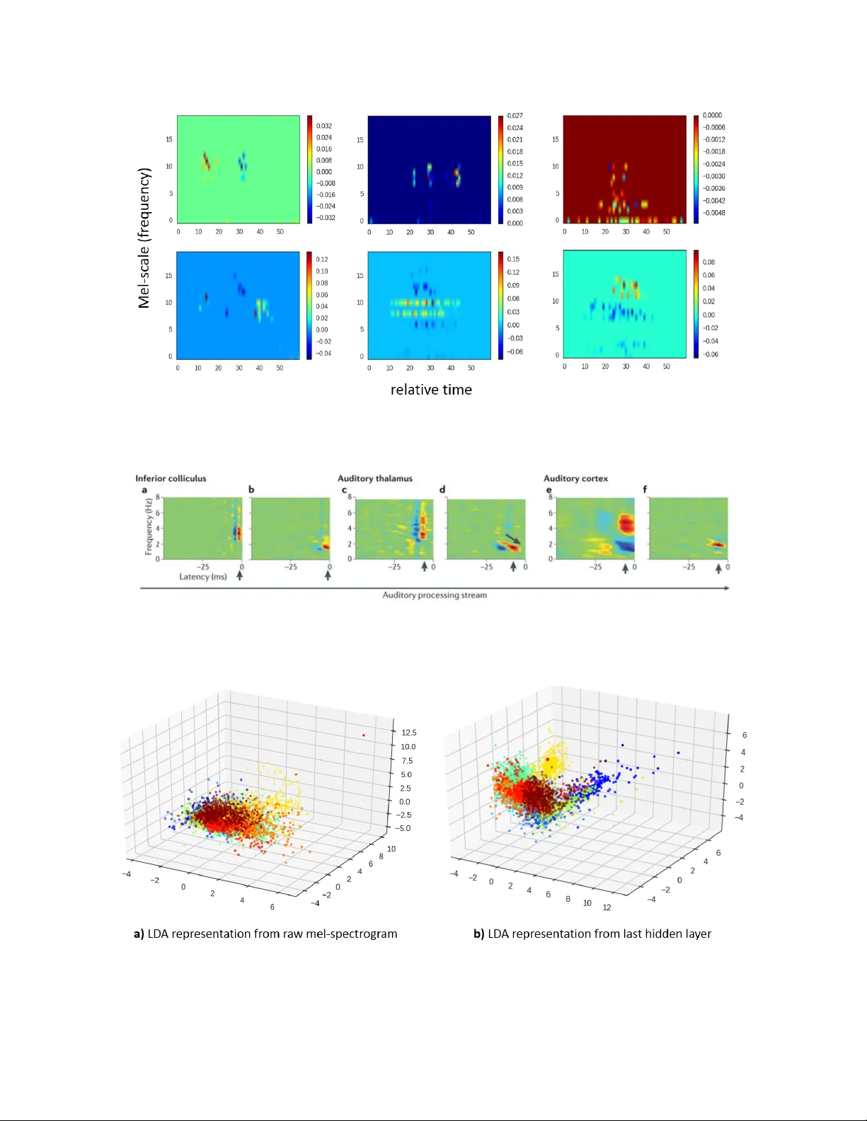
Con v olutional Neural Net w ork Ac hiev es Human-lev el Accuracy in Music Genre Classification Mingw en Dong Psyc hology , Rutgers Univ ersit y (New Brunswic k) mingw en.dong@rutgers.edu Abstract Music genre classification is one example of con tent-based analysis of m usic signals. T raditionally , h uman engineered features were used to automatize this task and 61% accuracy has b een achiev ed in the 10-genre classification. How ever, it’s still b elo w the 70% accuracy that humans could ac hieve in the same task. Here, we prop ose a new metho d that combines kno wledge of human perception study in music genre classification and the neuroph ysiology of the auditory system. The metho d works by training a simple conv olutional neural netw ork (CNN) to classify a short segment of the music signal. Then, the genre of a m usic is determined by splitting it into short segments and then combining CNN’s predictions from all short segments. After training, this metho d achiev es human-lev el (70%) accuracy and the filters learned in the CNN resemble the spectrotemp oral receptive field (STRF) in the auditory system 1 . In tro duction With the rapid dev elopment of digital tec hnology , the amount of digital m usic conten t increases dramatically ev eryday . T o give b etter music recommendations for the users, it’s essential to ha ve an algorithm that could automatically c haracterize the music. This pro cess is called Musical Information Retriev al (MIR) and one sp ecific example is music genre classification. Ho wev er, music genre classification is a v ery difficult problem b ecause the b oundaries b et ween different genres could b e fuzzy in nature. F or example, testing with a 10-w ay forced c hoices task, college students could ac hieve 70% classification accuracy after hearing 3 seconds of the m usic and the accuracy do esn’t impro ve with longer m usic [1]. Also, the num b er of lab eled data often is m uch smaller than the dimension of the data. F or example, GTZAN dataset 2 used in the curren t work contains only 1000 audio tracks, but eac h audio trac k is 30s long with a sampling rate 22,050 Hz. T raditionally , using human-engineered features like MFCC (Mel-frequency cepstral co efficien ts), texture, b eat and so on, 61% accuracy has b een achiev ed in the 10-genre classification task [1]. More recen tly , using PCA-whitened sp ectrogram as input, conv olutional deep b elief net work has ac hieved 70% accuracy in a 5-genre classification task. These results are reasonable but still not as go od as humans, suggesting there’s still space to impro ve. Psyc hophysics and ph ysiology study sho w that h uman auditory system works in a hierarchical wa y [2]. First, the ear decomp oses the contin uous sound wa v eform into different frequencies with higher precision on lo w frequencies. Then, neurons from low er to higher auditory structures gradually extract more complex sp ectro-temporal features with more complex sp ectro-temp oral receptiv e field (STRF) [3]. The features used by h uman auditory system for m usic genre classification probably rely on these STRFs. By having the sp ectrogram as input and the corresp onding genre as lab el, CNN will learn filters that extract features in the frequency and time domain. If these learned filters mimic STRFs in the human auditory system, they can extract useful features for music genre classification. Because music signal often is high-dimension in the time domain, having a CNN that fits the complete sp ectrogram of the music signal is not feasible. T o solve this problem, we used a ”divide-and-conquer” metho d: split the sp ectrogram of the music signal 1 All codes are av ailable at: https://github.com/ds7711/music_genre_classification 2 Av ailable at: http://marsyasweb.appspot.com/download/data_sets/ 1 Figure 1: Conv ert w av eform into mel-sp ectrogram and an example 3-second segment. Mel-spectrogram mimics how h uman ear works, with high precision in low frequency band and low precision in high frequency band. Note, the mel-sp ectrogram shown in the figures is already log transformed. in to consecutive 3-second segments, make predictions for each segment, and finally combine the predictions together. The main rational for this metho d is that humans’ classification accuracy plateaus at 3 seconds and go o d results were obtained using 3-second segmen ts to train conv olutional deep b elief netw ork [1] [4]. It also intuitiv ely makes sense b ecause differen t parts of the same music probably should b elong to the same genre. T o further reduce the dimension on the sp ectrogram, we used mel-sp ectrogram as the input to the CNN. Mel-sp ectrogram approximates ho w human auditory system works and can b e seen as the spectrogram smo othed in the frequency domain, with high precision in the low frequencies and low precision in the high frequencies [5] [6]. Data Pro cessing & Mo dels Data pre-pro cessing Eac h music signal is first conv erted from wa v eform into mel-sp ectrogram z i using Librosa library with 23ms time window and 50% ov erlap (figure 1). Then, the mel-sp ectrogram is log transformed to bring v alues at differen t mel-scale to the same range ( f ( z i ) = ln ( z i + 1)). Because mel-sp ectrogram is a biological-inspired represen tation [6], it has a simpler interpretation than the PCA-whitening metho d used in [4]. Net w ork Architecture 1. Input lay er: 64 * 256 neurons, corresp onds to 64 mel scales and 256 time windows(23ms, 50% ov erlap). 2. Conv olution la yer: 64 different 3 * 3 filters with a stride of 1. 3. Max p o oling la yer: 2 * 4. 4. Conv olution la yer: 64 different 3 * 5 filters with a stride of 1. 2 5. Max p o oling la yer: 2 * 4. 6. F ully connected lay er: 32 neurons that are fully connected to the neurons in the previous la yer. 7. Output lay er: 10 neurons that are fully connected to neurons in the previous la yer. F or 2D lay ers/filters, the first dimension corresp onds to the mel-scale and the second dimension corresp onds to the time. All hidden lay ers use RELU activ ation functions, the output la yer use softmax function, and the loss is calculated using cross-entrop y function. Drop out and L2 regularization were used to preven t extreme w eights. The mo del is implemen ted using Keras (2.0.1) with tensorflo w as back end and trained on a single GTX-1070 using sto c hastic gradien t descent. T raining & Prediction 1000 music tracks (con verted into mel-sp ectrogram) are evenly split into training, v alidation, and testing set with a ratio of 5 : 2 : 3. The training pro cedure is as following: 1. Select a subset of tracks from the training set. 2. Randomly sample a starting p oin t and take the 3-second contin uous segments from all selected tracks. 3. Calculate the gradients using back-propagation algorithm using the segmen ts as input and the lab els of the original m usic as target genres. 4. Up date the weigh ts using the gradients. 5. Rep eat the pro cedure un til classification accuracy on the cross-v alidation data set doesn’t improv e an ymore. During testing, all m usic (mel-sp ectrogram) are split in to consecutive 3-second segments with 50% ov er- lap. Then, for each segment, the trained neural netw ork predicts the probabilities of each genre. The predicted genre for eac h music is the genre with highest a veraged probability . Calculate the filters learned by the CNN After training, all musics are split into 3-second segments with 10% ov erlap. All the segments are then fed in to the trained CNN and in termediate outputs are calculated and stored. Then, we estimated the learned filters using the follo wing metho d: 1. Identify the range of input neurons (sp ecific section of the input mel-sp ectrogram) that could activ ate the target neuron at a sp ecific lay er. E.g., c ( l ) i,j indicates the neuron at lo cation ( i, j ) from the l th la yer. 2. Perform Lasso regression with the sp ecific section of the mel-sp ectrogram (reshap ed as a vector) as the regressors and the corresponding activ ations of the neuron c ( l ) i,j as the target v alues. 3. The fitted Lasso co efficients were reshap ed to estimate the learned filters. Results T o the b est of our knowledge, the current mo del is the first to achiev e human-lev el (70%) accuracy in the 10-genre classification task (figure 2). It’s 10% higher than that obtained in [1] and classifies 5 more different genres than [4] with similar accuracy . Classification accuracies v aries b y differen t genres. F rom the confusion matrix (figure 2), w e could see that the classification accuracy v aries a lot across differen t genres. Especially , the accuracies for country and ro c k genre are not only low er than the current a verage but also low er than those from [1] (whic h has o verall lo wer accuracy that our CNN). Because some imp ortan t h uman-engineered features used in [1] are the long-term feature like b eat and rhythm, this suggests coun try and ro c k music may ha ve c haracteristic features (e.g., b eat) that require longer time ( > 3 seconds) to 3 Figure 2: Confusion matrix of the CNN classification on testing set. capture and 3s segments used in our CNN are not long enough. One future direction is to explore how to use CNN to extract long-term features for classification and one p ossibilit y is to use another down-sampled mel-sp ectrogram of the whole audio as input. Another explanation is that coun try and ro c k share more features with the other music genres and are more difficult to classify in nature. Nonetheless, exp ert advice probably is required to improv e the classification accuracy on the coun try and ro ck genre. CNN learns filters like sp ectro-temp oral receptive field. Figure 2 shows some filters learned by the CNN’s 2nd max p ooling lay er and they’re qualitatively similar to the STRF obtained from physiological exp erimen ts (figure 4). T o visualize how these filters help classify the audios, we feed all the 3s segments from the testing set into the CNN and calculated the activ ations of the last hidden lay er. After this non-linear transformation, most testing data p oin ts b ecome linearly separable (figure 5). In contrast, the testing data points are muc h less separable when raw mel-sp ectrogram is used. These results together show that the CNN learns filters similar to the sp ectro-temporal receptive field observ ed in the brain. These filters transform the original mel-sp ectrogram into a representation where the data is linearly separable. Discussion By combining the kno wledge from h uman psyc hophysics study and neurophysiology , we used the CNN in a ”divide and conquer” w ay and classified the audio w av eforms in to differen t genres with h uman-level accuracy . The same technique may b e used to solve problems that share similar characteristics, for example, m usic tagging and artist identification using raw audio w av eform. With the current mo del, the genre of the music can b e extracted efficiently with h uman-level accuracy and used as features for recommending music to the users. 4 Figure 3: Filters learned by the CNN are s imilar to the STRF from ph ysiological exp erimen ts. Mel scale corresp onds to frequency and relativ e time corresponds to latency in figure 4. Figure 4: STRF obtained from physiological exp erimen ts. F rom left to right are the STRFs obtained from lo wer to higher auditory structures. Adapted from [3] with p ermission. Figure 5: Comparison b et ween the separability of the raw representation and last lay er representation of the CNN of the testing data. The axes are the first three comp onents when data is pro jected onto the directions obtained from linear discriminan t analysis (LDA). using training data. 5 References [1] George Tzanetakis and P erry Co ok. Musical genre classification of audio signals. IEEE T r ansactions on sp e e ch and audio pr o c essing , 10(5):293–302, 2002. [2] Jan Schn upp, Israel Nelken, and Andrew King. A uditory neur oscienc e: Making sense of sound . MIT press, 2011. [3] F r ´ ed ´ eric E Theunissen and Julie E Elie. Neural pro cessing of natural sounds. Natur e R eviews Neur o- scienc e , 15(6):355–366, 2014. [4] Honglak Lee, P eter Pham, Y an Largman, and Andrew Y Ng. Unsup ervised feature learning for audio classification using conv olutional deep b elief net works. In A dvanc es in neur al information pr o c essing systems , pages 1096–1104, 2009. [5] Douglas O’shaughnessy . Sp e e ch c ommunic ation: human and machine . Universities press, 1987. [6] Joseph W Picone. Signal modeling tec hniques in speech recognition. Pr o c e e dings of the IEEE , 81(9):1215– 1247, 1993. 6